Comparative Evaluation of Semi-Empirical Approaches to Retrieve Satellite-Derived Chlorophyll-a Concentrations from Nearshore and Offshore Waters of a Large Lake (Lake Ontario)

Abstract

Chlorophyll-a concentration (Chl-a) is commonly used as a proxy for phytoplankton abundance in surface waters of large lakes. Mapping spatial and temporal Chl-a distributions derived from multispectral satellite data is therefore increasingly popular for monitoring trends in trophic state of these important ecosystems. We evaluated products of eleven atmospheric correction processors (LEDAPS, LaSRC, Sen2Cor, ACOLITE, ATCOR, C2RCC, DOS 1, FLAASH, iCOR, Polymer, and QUAC) and 27 reflectance indexes (including band-ratio, three-band, and four-band algorithms) recommended for Chl-a concentration retrieval. These were applied to the western basin of Lake Ontario by pairing 236 satellite scenes from Landsat 5, 7, 8, and Sentinel-2 acquired between 2000 and 2022 to 600 near-synchronous and co-located in situ-measured Chl-a concentrations. The in situ data were categorized based on location, seasonality, and Carlson’s Trophic State Index (TSI). Linear regression Chl-a models were calibrated for each processing scheme plus data category. The models were compared using a range of performance metrics. Categorization of data based on trophic state yielded improved outcomes. Furthermore, Sentinel-2 and Landsat 8 data provided the best results, while Landsat 5 and 7 underperformed. A total of 28 Chl-a models were developed across the different data categorization schemes, with RMSEs ranging from 1.1 to 14.1 μg/L. ACOLITE-corrected images paired with the blue-to-green band ratio emerged as the generally best performing scheme. However, model performance was dependent on the data filtration practices and varied between satellites.

1. Introduction

The eutrophication of freshwater bodies is a global environmental concern. It is driven primarily by nutrient enrichment, most often accelerated by anthropogenic activities such as agricultural fertilizer application, wastewater discharge, and urbanization [1]. Cultural eutrophication promotes excessive growth of algae, leading to the deterioration of water quality and overall ecosystem health, and the loss of aquatic habitats [2]. In extreme cases, harmful algal blooms (HABs) occur through the rapid proliferation of algae, in particular cyanobacteria [3]. The occurrence of HABs is influenced by a complex interplay of biogeochemical and physical factors, including nutrient availability (mainly phosphorus and nitrogen), water temperature, and hydrodynamics [4].

In the western portion of Lake Ontario, algal blooms are a particular concern in nearshore areas including Hamilton Harbour (HH), the Toronto shoreline, and the Niagara River outlet [5]. Eutrophication in these areas is driven by excess nutrient runoff associated with rapid urbanization of the Greater Toronto Area [6] and surrounding agricultural and industrial activities [7]. Other contributing factors include nutrient-rich inflow from upstream Lake Erie via the connecting Niagara River [8], warmer water temperatures, and changes in circulation patterns [9], as well as ecological disturbances such as the invasion by nuisance mussels [9]. Given these rapidly changing dynamics, continued water quality monitoring of the nearshore and offshore waters of Western Lake Ontario (WLO) remains essential.

Traditional field-based water quality monitoring methods have played an integral role in tracking and assessing trophic changes in large lakes over the past several decades. While these methods are essential, they face limitations due to their high costs and personnel requirements, as well as their restricted spatial and temporal coverage. In this context, remote sensing (RS) techniques have emerged as a valuable complementary tool, enhancing traditional water quality monitoring with their ability to provide large-scale, frequent, and cost-effective observations of water bodies [10]. Multispectral satellites like Landsat 5, 7, 8, and Sentinel-2 are now extensively used for lake eutrophication monitoring at a global scale [11]. In RS research, chlorophyll-a (Chl-a) concentration, as the key photosynthetic pigment, is widely used to map algal abundance in diverse aquatic environments, including coastal areas, lakes, and rivers, providing a valuable tool for monitoring eutrophication trends [12,13,14]. The accuracy of Chl-a estimations depends highly on the applied atmospheric correction and the selection of appropriate retrieval algorithms [15]. By carefully addressing these aspects, RS can provide essential data on water quality trends and dynamics.

The estimation of Chl-a concentrations using multispectral satellite data has been growing in recent years [16]. This trend is notably tied to the launch of the Sentinel-2 satellite constellation in 2015, which added a red-edge band and increased spatial resolution down to 10 m. Achieving even higher spatial resolutions will require expanded data storage capacities, advanced sensors, or lower orbital altitudes. At present, medium spatial resolution, defined as 10 to 30 m, offers an adequate balance between detail and practicality for retrieving Chl-a concentrations from large water surfaces, including challenging nearshore areas where land adjacency can be an issue. Further improvements are expected in the near future with the anticipated launch of NASA’s 10 m super-spectral Landsat Next in 2030, which promises even finer spectral resolution, likely improving water colour remote sensing. A limited number of recent studies in the medium-spatial-resolution range have compared the performance of different atmospheric corrections and Chl-a concentration retrieval indexes (

Table 1. Summary of recently published studies comparing atmospheric corrections and Chl-a retrieval indexes.

Study Reference	Total Number of Chl-a Retrieval Indexes	Water Truthing			Imagery Matchups			Temporal Window of Matchups	Temporal Coverage of Matchups
		Number of Chl-a Data Points	Range of Chl-a Concentration (μg/L)	Radiometric Matchup Availability	Comparable * Sensors	Number of Scenes	Atmospheric Corrections
[17]	5	68–727	0–830	✓	OLI, MSI	N/A	ACOLITE, C2X, GRS, MEETC2, OC-SMART, Polymer, SeaDAS, iCOR	±3 and 30 h	N/A
[18]	3 5	34 51	0–181	✓	OLI MSI	2 3	DOS, ATCOR, DSF, EXP, L8SR	±5 days	2018–2019
[19]	3	1059–1668	N/A	✓	MSI	5–35	ACOLITE, C2RCC, iCOR, l2gen, Polymer, Sen2Cor	±3 and 24 h	2015–2016
[20]	6	351	1–65	✗	OLI	12	DOS	±2 and 5 days	2013–2015
[21]	9	146	0–309	✓	MSI	41	C2RCC, C2X, C2XC, Polymer	±3 h	2017–2021
[22]	6	97	0–250	✓	MSI	3	ACOLITE, C2RCC, GRS, iCOR, SeaDAS, Sen2Cor	±1 day	2018–2019
[23]	4	139	0–15	✓	OLI	61	SeaDAS, ACOLITE (DSF and EXP), C2RCC, iCOR	±1 h	2019–2021
[24]	17	120	0–13	✗	TM, ETM+	27	6S	±2 h	2000–2012
[25]	7	106	0–9	✗	MSI	13	ACOLITE (DSF)	Same day	2016–2017
[26]	17	102 127	2–63 2–40	✗	OLI MSI	48 44	SeaDAS, POLYMER, ACOLITE	Same day	2013–2020 2016–2020
[27]	5	54 54	3–7 2–7	✗	ETM+ OLI	8 8	LEDAPS L8SR	Same day	2013–2015
[28]	28	9–57	0–150	✓	MSI	N/A	ACOLITE, C2RCC, POLYMER, Sen2Cor	±3 days	2015–2017
[29]	9	30	1–6	✓	MSI	2	ELM	±1 h	2016–2017
[30]	11	39	0–0.6	✗	TM, ETM+, OLI	14	DOS	±9 days	2001–2003 2017–2019
[31]	5	97	0–80	✓	MSI	1	ACOLITE, C2RCC, C2X, iCOR, MAIN, Sen2Cor	Same day	2019
[32]	9	41	0–120	✓	MSI	41	C2RCC, C2X	±1 day	2018
[33]	4	39	50–250	✓	OLI	2	FLAASH	±2 h	2015–2016
[34]	9	350	0–6	✗	OLI	25	ACOLITE	±9 days	2014–2021
[15]	8	30	0–150	✓	MSI	7	ACOLITE, iCOR, Sen2Cor, C2RCC, C2X, POLYMER	±1 day	2018–2019
Current Study	27	205 217 127 51	0–137 0–52 0–80 0–31	✗	TM ETM+ OLI MSI	79 89 49 19	LEDAPS, LaSRC, Sen2Cor, ACOLITE, ATCOR, C2RCC, DOS 1, FLAASH, iCOR, Polymer, QUAC	±4 days	2000–2011 2000–2021 2013–2021 2016–2021

* Only limited to the list of sensors used in this study. Also, studies based on simulated satellite imagery are excluded from the table. Abbreviations in alphabetical order: 6S: Second Simulation of the Satellite Signal in the Solar Spectrum, ACOLITE: Atmospheric Correction for OLI Lite, ATCOR: Atmospheric and Topographic Correction, C2RCC: Case 2 Regional CoastColour, C2X: Case 2 eXtreme, C2X-COMPLEX, DOS: Dark Object Subtraction, DSF: Dark Spectrum Fitting, ELM: Empirical Line Method, ETM+: Enhanced Thematic Mapper Plus, FLAASH: Fast Line-of-sight Atmospheric Analysis of Hypercubes, GRS: Glint Remove Sentinel, LaSRC: Landsat Surface Reflectance Code, L8SR: Landsat 8 OLI Surface Reflectance, LEDAPS: Landsat Ecosystem Disturbance Adaptive Processing System, MAIN: Modified Atmospheric Correction for Inland Waters, MSI: Multispectral Instrument, OC-SMART: Ocean Colour–Simultaneous Marine and Aerosol Retrieval Tool, OLI: Operational Land Imager, QUAC: Quick Atmospheric Correction, SeaDAS: SeaWiFS Data Analysis System, Sen2Cor: Sentinel-2 Atmospheric Correction, TM: Thematic Mapper.

). Not surprisingly, these studies show that models to retrieve Chl-a concentration from satellite data tend to perform best for the data range and the region they were trained on.

The aim of this study is to build on previous studies mentioned in Table 1 by expanding the ranges of Chl-a retrieval indexes, atmospheric correction processors, satellites, and in situ matchup data included in our analyses. Specifically, we consider 27 Chl-a retrieval indexes, 11 atmospheric correction processors, four medium-spatial-resolution (10–30 m resolution) satellites, and 600 in situ matchup data points. Another novelty of our work is the categorization of the in situ Chl-a data based on seasonality, location, and Carlson’s Trophic State Index (TSI). This is followed by the derivation of separate regression-based models for each data category and satellite, which are then compared for their performance in retrieving Chl-a concentrations for both nearshore and offshore waters of Western Lake Ontario. The results of our work should inform future assessments of the changing spatial–temporal Chl-a distributions in Lake Ontario and other large lakes, thereby contributing to global efforts to use RS in water quality monitoring and management.

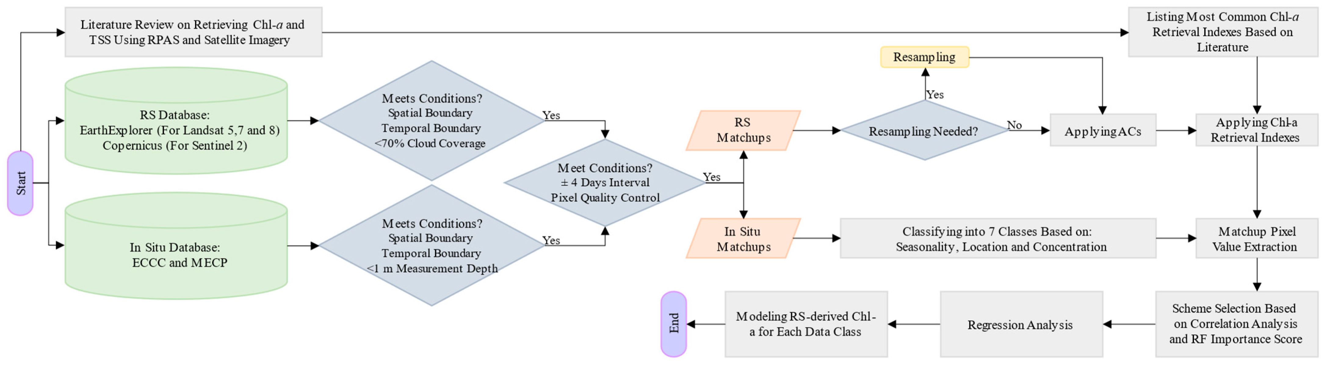
2. Materials and Methods

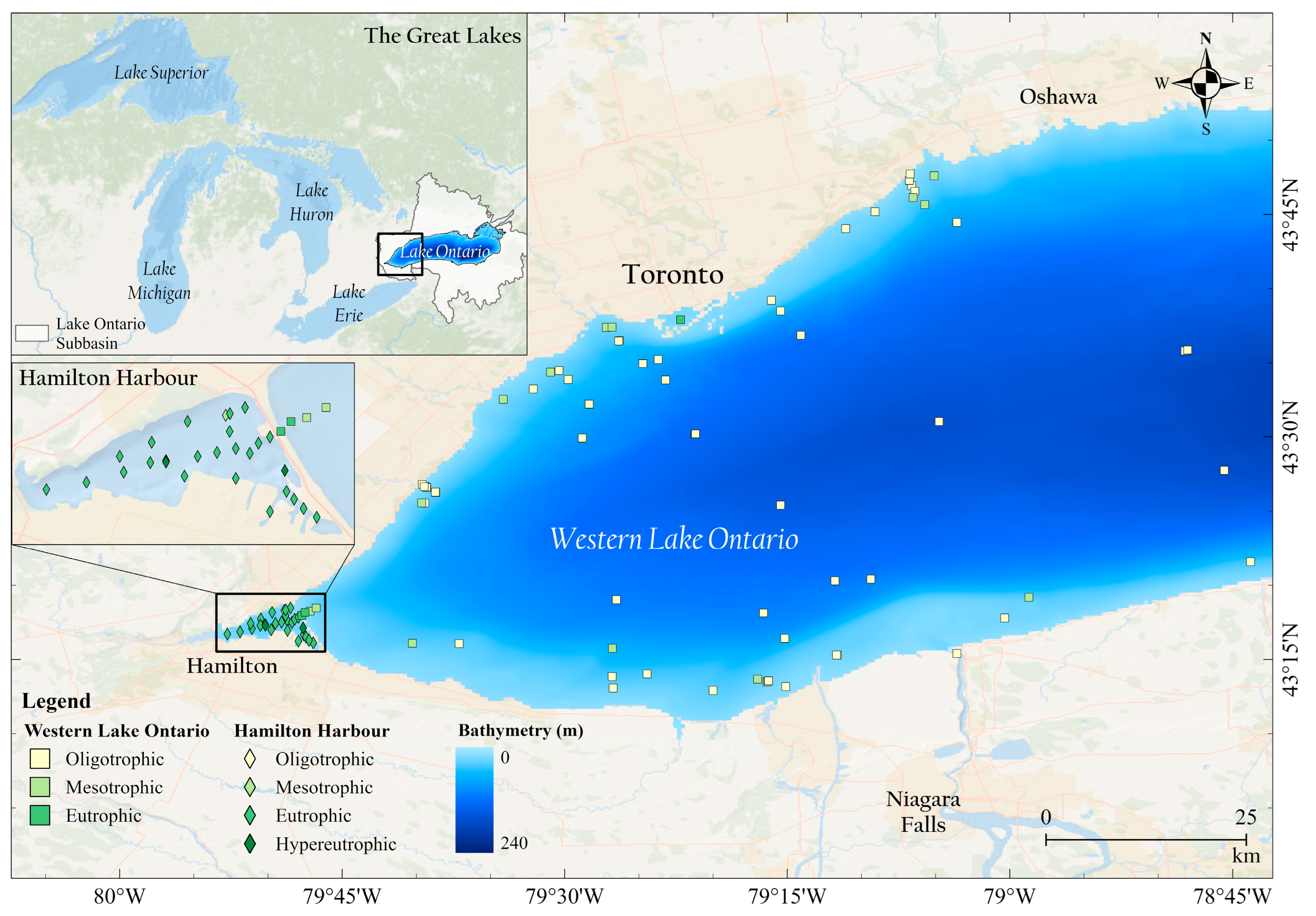
2.1. Study Site

Lake Ontario, the smallest and most easterly of the Great Lakes, ranks as the 13th largest lake in the world [35]. It has a drainage area of around 64,000 km², a surface area of 19,000 km², and a total volume of 1650 km³. The lake’s mean depth is 87 m, the maximum depth 244 m. The water residence time is approximately 6–8 years, and the lake’s shoreline extends over 1150 km. Our study focused on the western basin of Lake Ontario, abbreviated WLO, which represents a critical water resource for an estimated nine million people [9]. WLO covers about one-third of the entire surface area of Lake Ontario (Figure 1). Unlike for upstream Lake Erie, whole-lake assessments of RS-derived algal abundance remain limited for WLO. Also included in our study is Hamilton Harbour (HH), a 20 km² embayment at the western tip of WLO connected to the lake via a shipping channel. Since 1987, HH has been designated an Area of Concern under the Canada–US Great Lakes Water Quality Agreement. As a result, HH has a much higher density of water quality monitoring stations compared to WLO as can be seen in Figure 1.

Historically, WLO has experienced water quality issues due to both urban and rural non-point sources of nutrients and contaminants delivered to the lake by streams and storm sewers, as well as from upstream Lake Erie via the Niagara River [36]. The lake features mesotrophic to eutrophic nearshore zones and an oligotrophic offshore core [37]. In recent years, the total phosphorus (TP) concentration in the lake ranges on average from 6 to 8 μg/L, while the Chl-a concentration varies between 0 and 17 μg/L, depending on the location [38,39]. As expected, HH exhibits significantly higher TP and Chl-a concentrations, with Chl-a often exceeding 10 µg/L, that is, the threshold value commonly used to define an algal bloom [40].

The primary drivers of eutrophication in WLO and HH include rapid urbanization, and ecosystem and climate change [6,7,37], while invasive dreissenid mussels transform phosphorus into more readily bioavailable forms that promote algae growth [6,37,41]. The onset, duration, and intensity of algal growth are further influenced by environmental factors such as temperature, sunlight, and wind mixing [4,40]. The harmful effects of eutrophication in the region include water supply issues, human and pet health risks, diminished aquatic life, and economic impacts on tourism, recreational activities, and lakefront property value [2].

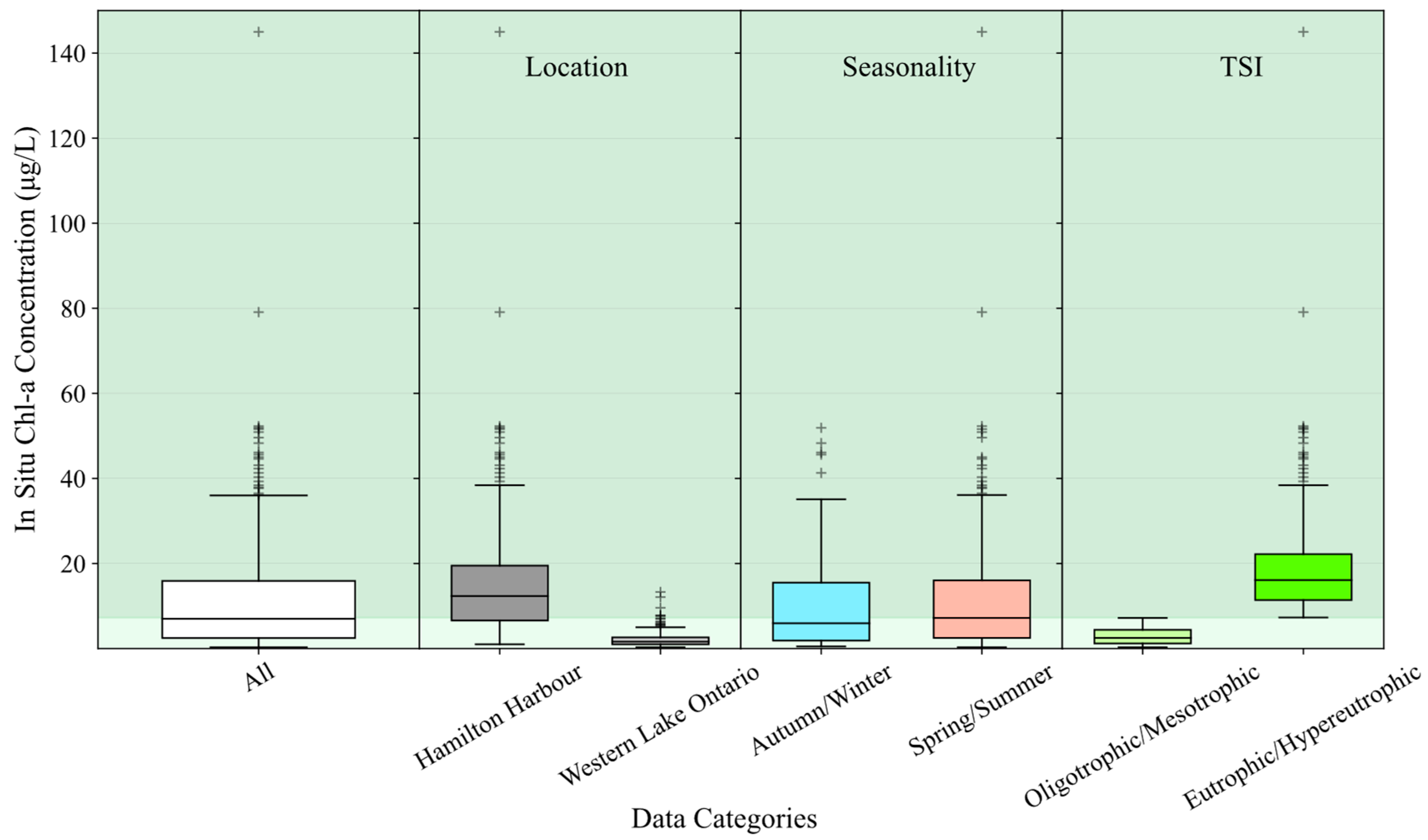
2.2. In Situ Chl-a Concentration Data

In situ matching data on Chl-a were extracted from the three databases identified in

Table 2. Overview of in situ data sources used in this study. ECCC = Environment and Climate Change Canada; MECP = Ministry of Environment, Conservation and Parks (Province of Ontario).

				Location
				WLO + HH	WLO	HH
Source	Organization	Published Data Availability	Chl-a Extraction Method	Fraction of Data (%)	Fraction within Study Site (%)
Hamilton Harbour Water Quality Data	ECCC	1987–2019	[42]	68%	5%	98%
Great Lakes Nearshore-Water Chemistry	MECP	2000–2017	[43,44]	15%	43%	2%
Great Lakes Water Quality Monitoring and Surveillance Data	ECCC	2000–Present	[45]	17%	52%	0%
				100%	100%	100%

. (Note: the hyperlinks to these databases are provided in the Code and Data availability Statement at the end of the paper). These databases have varying data availability periods and Chl-a concentration measurement methods (Table 2). The datasets were filtered based on two criteria: (i) a maximum time window of ±4 days between the in situ measurements and satellite image acquisition dates and (ii) a sampling water depth ranging from near surface to a maximum of 1 m. Because only a small portion of the datasets contained pheophytin-corrected records, the matchup analysis was conducted based on uncorrected Chl-a concentrations. In the few cases where uncorrected Chl-a concentration measurements were not available, pheophytin-corrected Chl-a data were utilized. This process resulted in 600 near-synchronous, co-located in situ matchups for WLO and HH, covering the period from 2000 up to 2022.

Of the total matchup data, 22% were collected during autumn/winter (September to February) and 78% in spring/summer (March to August). To categorize the data based on the Chl-a concentration data, we used Carlson’s Trophic State Index [TSI] [46] calculated as TSI = 9.81 × ln(Chl-a) + 30.6. Eutrophic to hypereutrophic conditions are defined by TSI ≥ 50, which is equivalent to Chl-a concentrations greater than 7.2 μg/L, while oligo-mesotrophic conditions correspond to TSI < 50 or Chl-a concentrations below 7.2 μg/L [47]. With this definition, 51% of the matchups fell in the oligotrophic/mesotrophic category, and the other 49% in the eutrophic/hypereutrophic category. The mean Chl-a concentration across all matchups was 10.5 μg/L, with a standard deviation of 11.3 μg/L. See Table S1 in Supplementary Materials for further details on the in situ Chl-a matchup data. A time-series plot of the in situ data is also presented in Figure S1 of Supplementary Materials colour-coded with their corresponding satellite matchups.

In this study, in situ Chl-a data were classified into four categories (Figure 2): the ‘all’ category includes all the data, the location category separates data between WLO and HH, the seasonality category has ‘Autumn/Winter (AW)’ and ‘Spring/Summer (SS)’ subcategories, and the TSI category divides the data among the ‘Oligotrophic/Mesotrophic (OM)’ and ‘Eutrophic/Hypereutrophic (EH)’ subcategories. The categorization helps in evaluating the performance of each scheme and to better understand the factors that influence the accuracy of satellite-derived Chl-a concentration estimations. For instance, a chi-squared test from in situ measurements revealed a significant association between location and the TSI categories (${\chi }^2=235$, $p<0.001$, $V=0.63$), which reflects the typically more eutrophic conditions encountered in HH than WLO.

2.3. Remote Sensing Data

In this study, images from four medium-spatial-resolution satellites were used: Landsat 5, 7, 8, and Sentinel 2 A/B. Our study area is covered by paths 17/18 and row 30 of Landsat and tiles T17TNJ, T17TNH, T17TPH, and T17TPJ of Sentinel-2, encompassing two Landsat and four Sentinel-2 scenes. Each of these satellites possesses unique features and characteristics that are summarized in

Table 3. Overview of Landsat 5, 7, 8, and Sentinel-2.

		Landsat 5	Landsat 7	Landsat 8–9	Sentinel-2 A/B
Sensor		TM	ETM+	OLI and TIRS (OLI-2 and TIRS-2)	MSI
Operating Dates		1984–2013	1999–Present	2013–Present	2015–Present
No. of Bands		7	8	11 (9 OLI, 2 TIRS)	13
Spatial Res. (m)		15 (panchromatic band), 30, 120 (thermal)	15 (panchromatic band), 30, 60 (thermal)	15 (panchromatic band), 30, 100 (TIRS)	10 (4 bands), 20 (6 bands), 60 (3 bands)
Temporal Res. (days)		16	16	8 (Landsat 8 and 9 combined)	~5 (Sentinel-2 A and B combined)
Radiometric Res. (bit)		8	8	12 (14 for Landsat 9)	12
Spectral Range (nm)		450–2350 10,400–12,500 (thermal)	450–2350 10,400–12,500 (thermal)	430–2300 (OLI) 10,600–12,500 (TIRS)	443–2190
Chl-a Retrieval Bands in nm (central wavelength)	${\lambda }_{UB}$	-	-	433–453 (443)	433–453 (443)
	${\lambda }_B$	450–520 (485)	450–515 (483)	450–515 (482)	458–523 (490)
	${\lambda }_G$	520–600 (560)	520–605 (565)	525–600 (562)	543–578 (560)
	${\lambda }_R$	630–690 (660)	630–690 (660)	630–680 (655)	650–680 (665)
	${\lambda }_{RE1}$	-	-	-	698–713 (705)
	${\lambda }_{RE2}$	-	-	-	733–747 (740)
	${\lambda }_{RE3}$	-	-	-	773–793 (783)
	${\lambda }_{NIR1}$	760–900 (830)	775–900 (837)	-	785–900 (842)
	${\lambda }_{NIR2}$	-	-	845–885 (865)	935–955 (865)

Abbreviations in alphabetical order: G: Green, B: Blue, NIR: Near-Infrared, R: Red, RE: Red-Edge, TIRS: Thermal Infrared Sensor, UB: Ultra-Blue.

. The differing spatial, spectral, radiometric, and temporal resolutions of these satellites impact their capacity to estimate Chl-a concentrations in water bodies [11]. The literature suggests that the inclusion of an ultra-blue band at approximately 440 nm and the improved signal-to-noise ratio (SNR) of Landsat 8 and Sentinel-2 yield more accurate Chl-a concentration estimates compared to the previous generation satellites [48,49].

In total, 236 matchup scenes were selected after quality control for cloud, snow, shadow, and overlapping land pixel artefacts. The scenes were distributed as follows among the different satellites: Landsat 5: 79 scenes; Landsat 7: 89 scenes; Landsat 8: 49 scenes; and Sentinel-2: 19 scenes. Each scene contained at least one high-quality pixel coinciding with an in situ measurement location. Most of the downloaded RS scenes were acquired within ±1 day of the in situ sampling dates and at most within ±4 days. Such close temporal matching is important given the rapidly changing algal patterns often observed in lakes [4].

2.4. Atmospheric Correction Processors

Atmospheric correction is a crucial step to accurately retrieve Chl-a concentrations from satellite data because at-sensor radiance is affected by atmospheric gaseous molecules and aerosols, especially at shorter wavelengths [22,50], as well as by other factors such as air–water interface, wind, and sunglint [51]. While some atmospheric correction processors considered here can correct sunglint-related effects to a degree, an investigation of these effects is beyond the scope of our study.

The availability of atmospheric correction processors varies across the four satellites. For Landsat 5 and 7, both Level-1 and Level-2 (LEDAPS-corrected) products are publicly available, and the Level-1 imagery is also compatible with the ACOLITE, ATCOR, DOS1, FLAASH, and QUAC processors. In the case of Landsat 8, Level-1 and Level-2 (LaSRC-corrected) are publicly available through the EarthExplorer data hub, and the satellite is compatible with all the above-mentioned processors plus C2RCC and iCOR. Finally, Sentinel-2, through the Copernicus data hub, freely offers Level-1 and Level-2 (Sen2Cor-corrected) products, with compatibility with the ACOLITE, C2RCC, DOS1, iCOR, and Polymer processors. Although atmospherically corrected Sentinel-2 products (MSIL2A) are available for download, their global coverage only commenced in late 2018. Hence, we applied the Sen2Cor processors independently on Sentinel-2 Level-1 images using the ESA SNAP software (version 9.0.0). Also of note, ACOLITE includes two correction methods: Dark Spectrum Fitting (DSF, the processor’s default) and Exponential Extrapolation (EXP). Because DSF has been reported as the better choice for aquatic studies [18,23], it was used in this study. Table S2 in Supplementary Materials summarizes the atmospheric correction methods utilized in this study.

2.5. Chl-a Retrieval Indexes

The Chl-a retrieval methods for satellite imagery broadly fall into four groups: empirical, semi-empirical, analytical, and semi-analytical [48]. In this study, we focus on semi-empirical methods. Semi-empirical models analyze the inherent optical properties (IOPs) of optically active constituents (OACs) by integrating water spectral theory with statistical techniques [13]. They offer ease of implementation, reproducible results, and reasonable accuracy without overfitting risk, all achieved by selecting the most suitable band combinations for retrieving water quality parameters [50]. Here, the choice of semi-empirical methods was also dictated by the limited availability of in situ matchup data for our study site.

Upon conducting an extensive literature review, 27 commonly used semi-empirical Chl-a indexes were selected. These indexes employ various band combinations to retrieve the Chl-a concentration from the matching vector of pixel values. The applicability of these indexes varies across different satellite platforms. Notably, Sentinel-2 and Landsat 8 demonstrate broader compatibility owing to their superior spectral resolution, particularly in ultra-blue, red-edge, and narrow near-infrared bands. The selected indexes, together with the corresponding formulas (band math), names, references, and applicability, are found in

Table 4. Chl-a retrieval indexes used in this study.

		Index Code	Band Math	Also Known As	Supported Sensors	Original Reference(s)
2BDA	2-Band Ratios	$I_1$	$\frac{UB}{B}$	-	OLI, MSI	N/A
		$I_2$	$\frac{UB}{G}$	OC3E	OLI, MSI	[52,53,54]
		$I_3$	$\frac{B}{G}$		TM, ETM+, OLI, MSI
		$I_4$	$\frac{NIR1}{G}$	-	TM, ETM+, MSI	[55]
		$I_5$	$\frac{NIR2}{G}$		OLI, MSI
		$I_6$	$\frac{B}{R}$	-	TM, ETM+, OLI, MSI	[56,57]
		$I_7$	$\frac{G}{R}$	-	TM, ETM+, OLI, MSI	[58,59,60]
		$I_8$	$\frac{RE1}{R}$	-	MSI	[61,62,63,64]
		$I_9$	$\frac{RE2}{R}$	-	MSI	[64]
		$I_{10}$	$\frac{NIR1}{R}$	-	TM, ETM+, MSI	[65,66]
		$I_{11}$	$\frac{NIR2}{R}$		OLI, MSI
	Normalized Indexes	$I_{12}$	$\frac{G-R}{G+R}$	NDGRI	TM, ETM+, OLI, MSI	[67]
		$I_{13}$	$\frac{RE1-R}{RE1+R}$	NDCI	MSI	[68]
		$I_{14}$	$\frac{RE2-R}{RE2+R}$	-	MSI	N/A
		$I_{15}$	$\frac{RE3-R}{RE3+R}$	-	MSI	N/A
		$I_{16}$	$\frac{NIR1-R}{NIR1+R}$	NDVI	TM, ETM+, MSI	[69]
		$I_{17}$	$\frac{NIR2-R}{NIR2+R}$		OLI, MSI
3BDA		$I_{18}$	$\frac{B-R}{G}$	BRG Index or KIVU	TM, ETM+, OLI, MSI	[70,71]
		$I_{19}$	$RE1-\frac{R+RE2}{2}$	Toming	MSI	[72,73]
		$I_{20}$	$RE1-\frac{R+RE3}{2}$	-	MSI	N/A
		$I_{21}$	$\left[\frac{1}{R}-\frac{1}{RE1}\right]\times RE2$	-	MSI	[74,75]
		$I_{22}$	$\frac{\left[\frac{1}{R}-\frac{1}{RE1}\right]}{\left[\frac{1}{RE2}-\frac{1}{RE1}\right]}$	-	MSI	[76]
	FLH/RLH-based Formulation	$I_{23}$	$G-UB-\left(\frac{{\lambda }_G-{\lambda }_{UB}}{{\lambda }_R-{\lambda }_{UB}}\right)\left(R-UB\right)$	CI	OLI, MSI	[77]
		$I_{24}$	$G-R-\left(\frac{{\lambda }_G-{\lambda }_R}{{\lambda }_B-{\lambda }_R}\right)\left(B-R\right)$	-	TM, ETM+, OLI, MSI	N/A
		$I_{25}$	$RE1-R-\left(\frac{{\lambda }_{RE1}-{\lambda }_R}{{\lambda }_{RE2}-{\lambda }_R}\right)\left(RE2-R\right)$	MCI or SLH	MSI	[78,79]
		$I_{26}$	$RE1-R-\left(\frac{{\lambda }_{RE1}-{\lambda }_R}{{\lambda }_{NIR2}-{\lambda }_R}\right)\left(NIR2-R\right)$	MPH	MSI	[80]
4BDA		$I_{27}$	$\frac{NIR2-R}{B+G}$	SABI	OLI, MSI	[81]

Abbreviations in alphabetical order: 2BDA: 2-Band Algorithm, 3BDA: 3-Band Algorithm, 4BDA: 4-Band Algorithm, FLH: Fluorescence Line Height, MCI: Maximum Chlorophyll Index, MPH: Maximum Peak Height, NDCI: Normalized Difference Chlorophyll Index, NDGRI: Normalized Difference Green and Red Index, NDVI: Normalized Difference Vegetation Index, RLH: Reflectance Line Height, SLH: Scattering Line Height.

. Next, these indexes were applied to atmospherically corrected images, selecting the most important feature and atmospheric correction processor, followed by regression analyses between the retrieved pixel values and in situ Chl-a concentrations.

2.6. Performance Metrics

Correlation was assessed using Pearson’s $r$ and Spearman’s $\rho$ coefficients. The former was calculated as

$$r=\frac{\sum \left[\left(I-\overline{I}\right)\left(\log \left(chl{a}_{meas}\right)-\overline{\log \left(chl{a}_{meas}\right)}\right)\right]}{\sqrt{\sum \left[{\left(I-\overline{I}\right)}^2\right]\times \sum \left[{\left(\log \left(chl{a}_{meas}\right)-\overline{\log \left(chl{a}_{meas}\right)}\right)}^2\right]}}$$

(1)

where $I$ is the spectral index (i.e., the independent variable or predictor) and $chl{a}_{meas}$ is the measured in situ Chl-a concentration (i.e., the dependent variable or response). Spearman’s $\rho$ coefficient was given by

$$\rho =1-\frac{6\sum d^2}{n\left(n^2-1\right)}$$

(2)

where $d$ is the difference between a pair of ranks and $n$ is the number of data. For both correlation coefficients, the values range from −1 to 1. Statistically, a significant correlation exists when the absolute values of $r$ and $\rho$ fall within the range 0.5 to 1.

Regression analysis is often used to assess the performance of semi-empirical RS-derived models against the water-truth parameters. Here, we employed the following metrics to assess the models’ predictive capability [26,51,82]:

$$RMSLE=\sqrt{\frac{1}{n}\sum \left\{{\left[\log \left(chl{a}_{meas}\right)-\log \left(chl{a}_{mod}\right)\right]}^2\right\}}$$

(3)

$$RMSE \left(\mu \mathrm{g}/\mathrm{L}\right)=\sqrt{\frac{1}{n}\sum \left[{\left(chl{a}_{meas}-chl{a}_{mod}\right)}^2\right]}$$

(4)

$$Bias={10}^{\left\{\frac{1}{n}\sum \left[\log \left(\frac{chl{a}_{meas}}{chl{a}_{mod}}\right)\right]\right\}}$$

(5)

$$MAE={10}^{\left[\frac{1}{n}\sum \left|\log \left(\frac{chl{a}_{meas}}{chl{a}_{mod}}\right)\right|\right]}$$

(6)

$$MAPE \left(\%\right)=100\times \frac{1}{n}\sum \left[\frac{chl{a}_{meas}-chl{a}_{mod}}{chl{a}_{meas}}\right]$$

(7)

$$MDAPE \left(\%\right)=100\times \tilde{r}$$

(8)

where $\tilde{r}$ is the median of $\frac{\left|chl{a}_{mod}\left(i\right)-chl{a}_{meas}\left(i\right)\right|}{chl{a}_{meas}\left(\left(i\right)\right)}$ where $i=1,\dots ,n$

$$\epsilon \left(\%\right)=100\times \left({10}^Y-1\right)$$

(9)

where $Y$ is the median of $\left|\log \left(\frac{chl{a}_{meas}}{chl{a}_{mod}}\right)\right|$

$$\beta \left(\%\right)=100\times \left({10}^Z-1\right)\times sing\left(Z\right)$$

(10)

where $Z$ is the median of $\left[\log \left(\frac{chl{a}_{meas}}{chl{a}_{mod}}\right)\right]$

$$R^2=1-\frac{\sum \left\{{\left[\log \left(chl{a}_{meas}\right)-\log \left(chl{a}_{mod}\right)\right]}^2\right\}}{\sum \left\{{\left[\log \left(chl{a}_{meas}\right)-\overline{\log \left(chl{a}_{meas}\right)}\right]}^2\right\}}$$

(11)

where the $\sum$ signs above denote summation over i = 1, …, n. Generally, lower absolute values for the root-mean-squared logarithmic error (RMSLE), root-mean-squared error (RMSE), and mean absolute error (MAE) indicate better model performance, while higher values for R² imply better goodness of fit. Bias values near one indicate little bias, while values above and below one indicate average under- and over-prediction, respectively. Mean absolute percentage error (MAPE) and median absolute percentage error (MDAPE) measure the percentage error, with 0% implying perfect prediction. Similarly, the metrics $\epsilon$ and $\beta$ report relative errors, with 100% indicating an accurate median prediction while values above (below) 100% indicate model overestimation (underestimation). Using these metrics together enabled a comprehensive model performance assessment. Note that, for some of the metrics, a base-10 logarithmic transformation was used to enhance data normality and reliability [51]. The overview of data and methodology and key steps is summarized in Figure 3.

2.7. Scheme Selection

In order to perform the regression analysis and develop an RS-derived Chl-a (${\mathrm{Chla}}_{\mathrm{RS}}$) model for a given scenario (i.e., a given satellite and data category combination), the primary (most significant) feature (i.e., the retrieval index) as well as atmospheric correction processor for the ${\mathrm{Chla}}_{\mathrm{RS}}$ model were first identified. Random Forest (RF) scoring was primarily used in the selection of the optimal scheme for each satellite and data category. While in most cases the top-ranked RF importance score determined the best scheme (20 out of 28 scenarios), we occasionally selected the second-ranked scheme when it demonstrated significantly higher correlation coefficients (for both Pearson’s $r$ and Spearman’s $\rho$).

3. Results

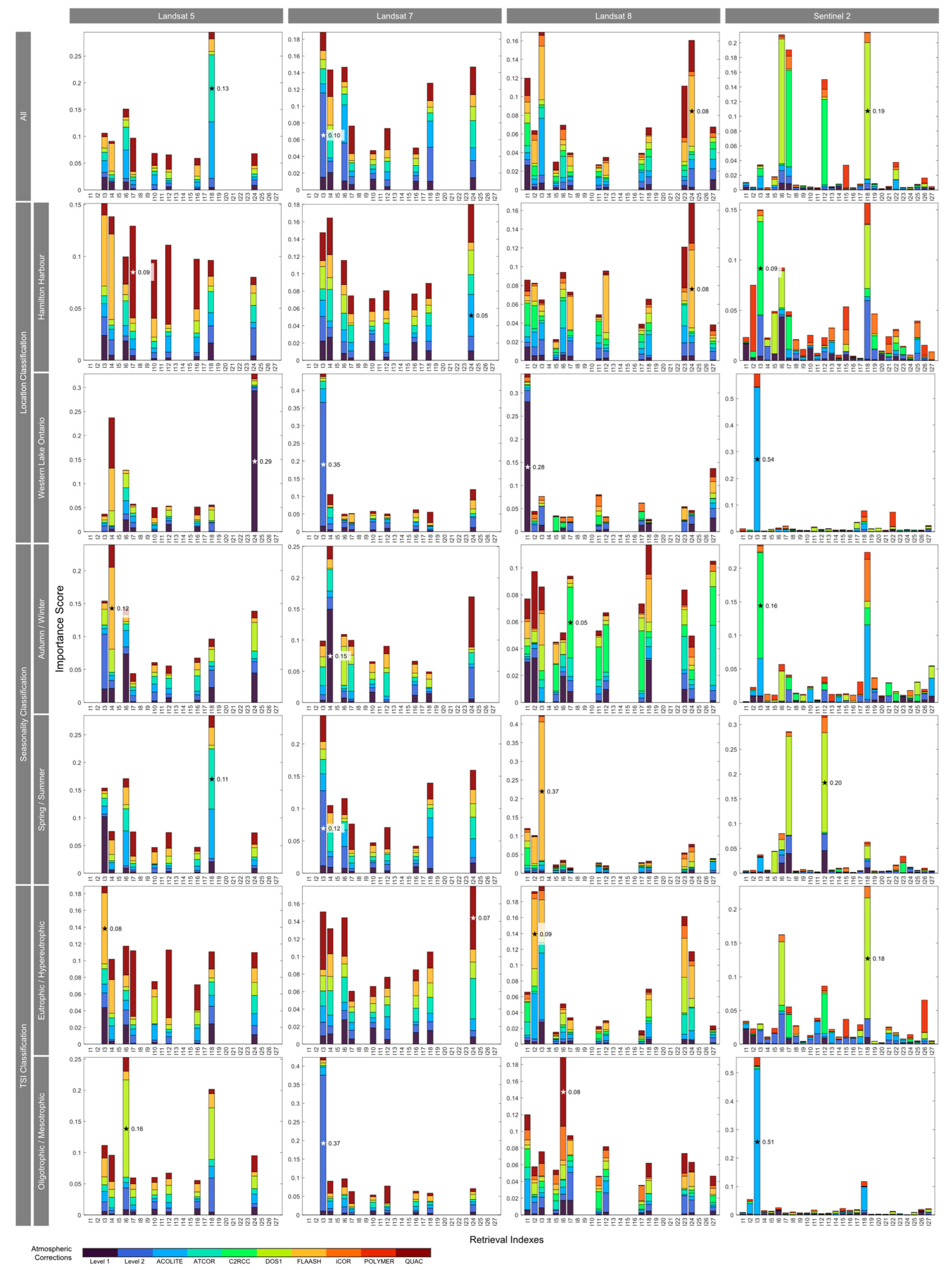
3.1. Feature Importance Scoring by Random Forest

Feature importance analysis by RF ranks the significance of input variables in predicting the target output through a tree-based learning mechanism. In this study, RF was used to quantify the importance of the different combinations of retrieval indexes and atmospheric correction methods (i.e., the schemes) for the different satellites and data categories (i.e., the different scenarios). We used the RandomForestRegressor and SimpleImputer from the sklearn library [83] in Python to model the scheme importance and handle missing data, respectively. The SimpleImputer was configured to impute missing values using the mean strategy. We then trained a RandomForestRegressor model equipped with 100 estimators (individual decision trees) and set to a random state of 42 (as the seed value for the algorithm’s random number generator) to ensure reproducibility. The feature importance scores were directly extracted from the fitted model, providing a quantitative measure of each scheme’s contribution to the prediction accuracy.

The results, shown in Figure 4, exhibit notable differences in scheme importance across scenarios. While in some scenarios a single scheme clearly dominated, indicating a distinct preference for that specific scheme, in other scenarios multiple schemes yielded comparable importance. Among the atmospheric correction processors, QUAC and FLAASH tended to dominate for Landsat 5 and 8, Level-2 (LEDAPS) for Landsat 7, DOS1, C2RCC, and ACOLITE for Sentinel-2. Generally, FLAASH, DOS1, Level-2, and QUAC products performed best. Out of the 28 scenarios, Level-1 (uncorrected data) only emerged as the top product in 3 scenarios, hence underscoring the critical importance of atmospheric correction prior to processing satellite data. Interestingly, iCOR and Polymer were never among the top processors, although they showed relatively high importance in several scenarios. In terms of the Chl-a indexes, I₃, I₄, and I₁₈ were favoured by Landsat 5 and 7, I₁, I₃, I₆, and I₂₄ by Landsat 8, and I₃ and I₁₈ by Sentinel-2. Overall, I₃ (blue-to-green ratio) emerged as the preferred index for Chl-a concentration prediction across all satellites and data categories. These results should help inform the preliminary selection of retrieval indexes and suitable atmospheric correction processors when developing multiple regression or machine learning models in future RS studies aimed at analyzing spatial–temporal Chl-a trends in lakes and other surface water bodies.

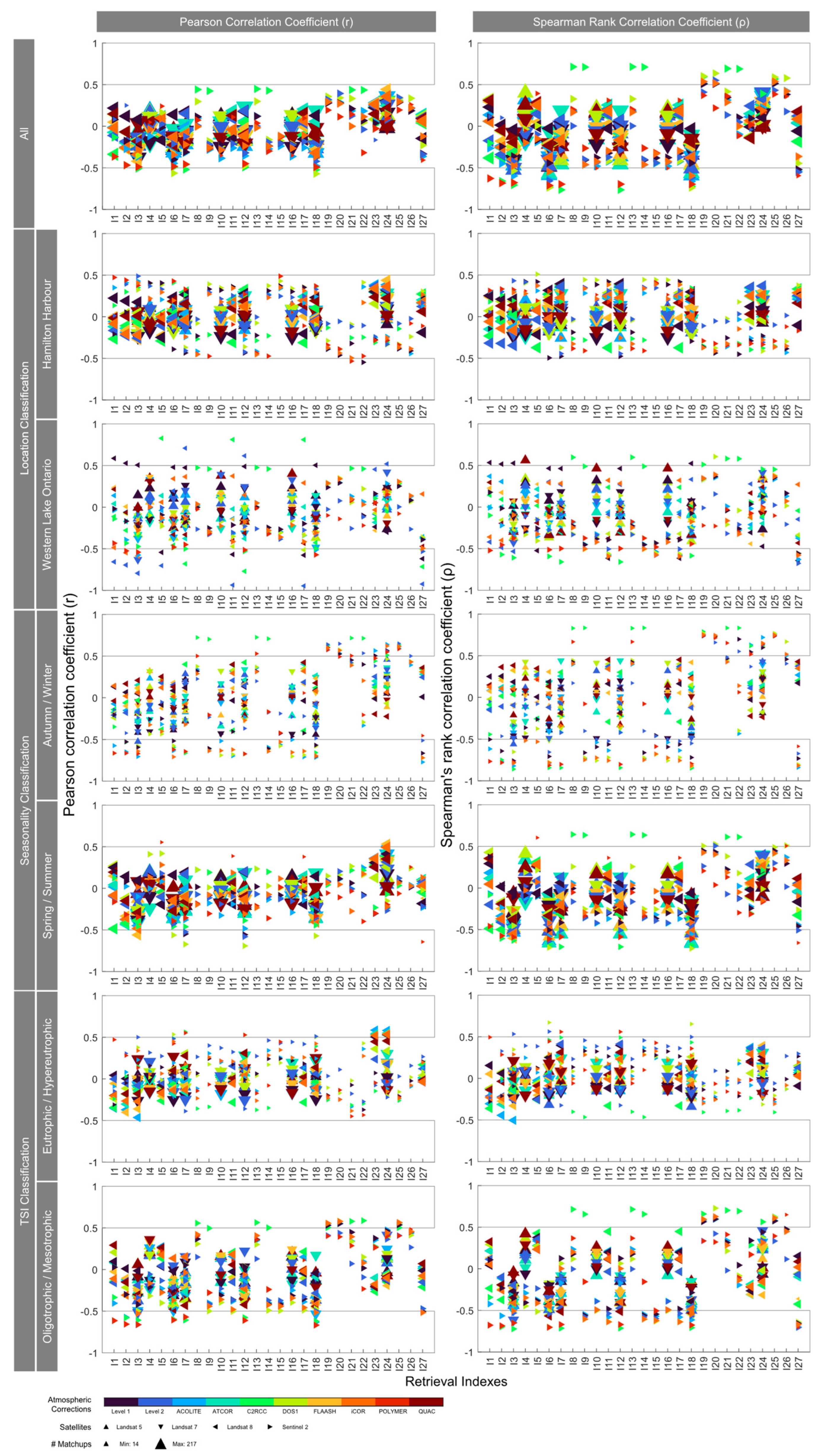
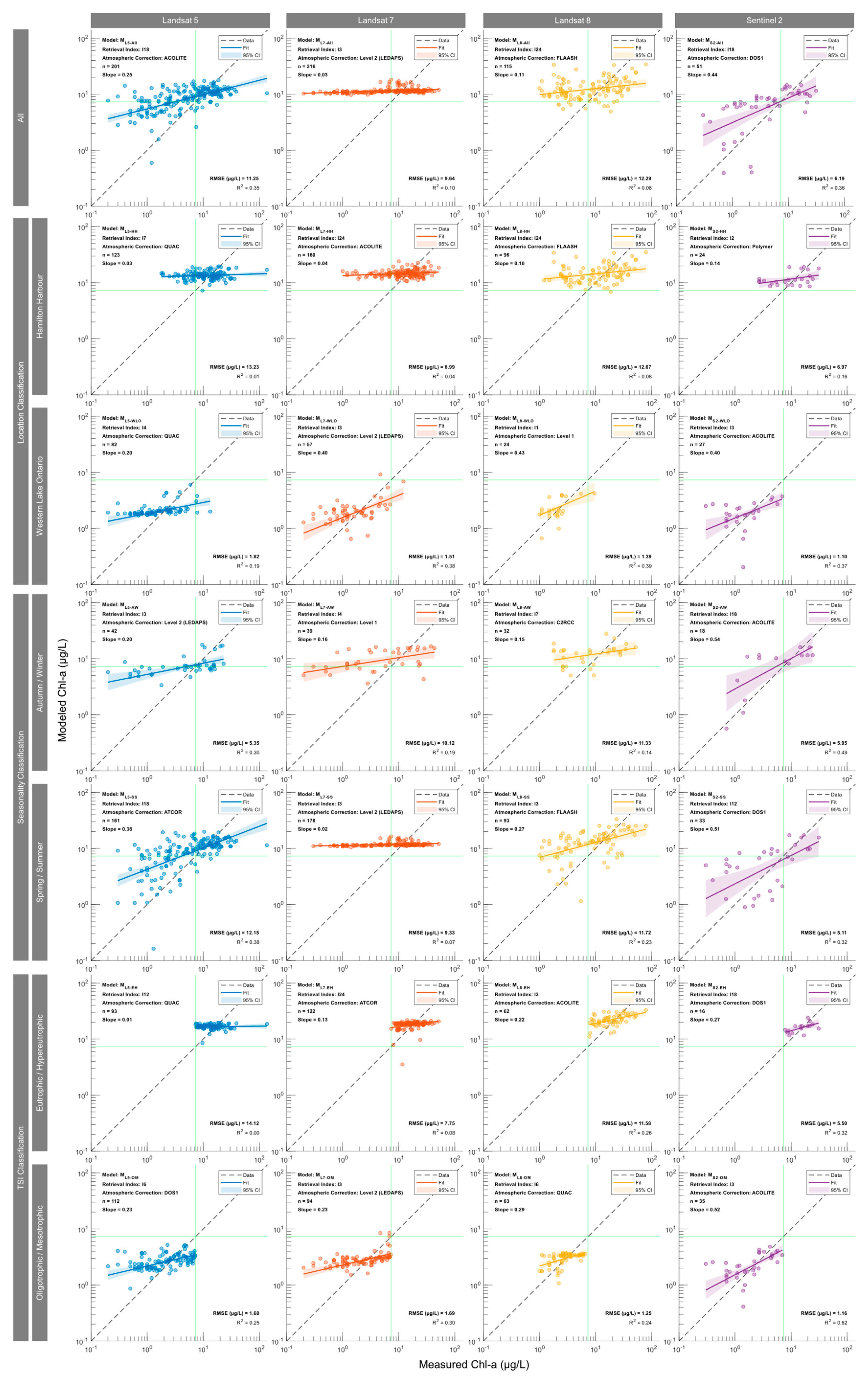
3.2. Correlation and Regression Analyses

Correlation analysis was applied to examine relationships between in situ Chl-a concentrations and the corresponding spectral indexes derived from atmospherically corrected matchup pixels [84,85]. Figure 5 presents the resulting correlation coefficients for the retrieval indexes. A heatmap of only R² values from the correlation analysis is also provided in Figure S2 of the Supplementary Materials. These figures reveal that some indexes, such as I₂₇, exhibited an overall negative correlation, that is, an increase in the index value corresponds to a decrease in Chl-a concentration. Conversely, indexes such as for example I₂₆, exhibited a positive correlation for most scenarios, indicating a direct relationship between the index value and the Chl-a concentration. However, the majority of correlation metrics were in the range ±0.5, indicating statistically insignificant correlation. Furthermore, the results indicated that, regardless of the data category, both Sentinel-2 and Landsat 8 constantly had superior correlations compared to the other satellites. Of note is that while correlation analysis shows the strength and direction of the relationship, it does not provide insights into the models’ prediction accuracy or biases.

To select the optimal scheme (combination of atmospheric correction processor and Chl-a retrieval index) for each scenario (data category and satellite), we primarily relied on the RF importance scores because they offer a more robust feature selection metric for regression models compared to traditional correlation coefficients. Therefore, for each scenario, we initially ranked schemes by RF importance score. The top-ranked scheme was then selected, unless the second-ranked scheme demonstrated significantly higher correlation coefficients (for both Pearson’s $r$ and Spearman’s $\rho$). Out of 28 scenarios, the optimal schemes of 20 scenarios were directly determined by the highest RF importance score, while the remaining 8 had the second-highest RF score but ranked significantly better based on the correlation coefficients.

Next, a linear regression was fitted between the scheme-derived and matchup Chl-a concentrations to generate a predictive equation for Chl-a. The predicted versus matchup (measured) Chl-a concentrations are plotted in Figure 6. Details on the performance metrics as well as the regression equations, are presented in Table S3 of Supplementary Materials. The plots in Figure 6 are colour-coded by satellite (Landsat 5, 7, 8, and Sentinel-2, left to right) and identify the four in situ data categories defined in Section 2.2: all (no filtering), location (HH or WLO), seasonality (AW or SS), and TSI (OM or EH). The retrieval index and atmospheric correction processor as well as the values for the matchup count, regression slope, RMSE, and R² are also shown on the plots.

Landsat 5 and 7 data typically exhibited higher RMSE, from 1.5 (WLO) to 14.1 µg/L (EH). In contrast, Landsat 5’s HH and EH categories had nearly zero slopes, indicating ineffective predictive power. The best performance for Landsat 5 occurred in the SS category, with a slope and R² of 0.38, indicating overprediction and underprediction at low and high concentrations, respectively. The Landsat 7 models generally yielded low slopes, except for the WLO location subcategory model (slope: 0.40, R²: 0.38, RMSE: 1.5 µg/L). Landsat 8 models had slopes between 0.11 and 0.43 and RMSE between 1.3 and 12.7 µg/L. The best Landsat 8 model for WLO data yielded a slope of 0.43, RMSE of 1.4 µg/L, and R² of 0.39. Sentinel-2 models generally outperformed those for the other satellites, with slopes from 0.14 to 0.54, RMSE from 1.2 to 7.0 µg/L, and R² from 0.16 to 0.52. We attribute this to Sentinel-2’s superior spatial, spectral, and radiometric resolution. Most models for Sentinel-2 were atmospherically corrected using ACOLITE or DOS1. For the subcategory OM, Sentinel-2 exhibited the best performance (slope: 0.52, RMSE: 1.2 µg/L, R²: 0.52) and hence provided the best option for the lower Chl-a concentration range due to its higher sensitivity (higher radiometric resolution) to variations in water colour.

4. Discussion

4.1. Performance of Satellites

Overall, compared to Landsat 5 and 7, Sentinel-2 and Landsat 8 demonstrate superior performance, with RMSLE values ranging from 0.18 (M_L8-WLO and M_L8-OM) to 0.49 (M_L8-All) for Landsat 8, and 0.15 (M_S2-EH) to 0.38 (M_S2-All) for Sentinel-2. The average RMSLE for all seven scenarios is 0.34 for Landsat 8 and 0.27 for Sentinel-2, suggesting a slightly better performance for Sentinel-2. In contrast, Landsat 5 and 7 have RMSLE ranges of 0.21–0.41 and 0.18–0.52, respectively. The other performance metrics similarly imply the superior performance of Sentinel-2, followed by Landsat 8. For example, Sentinel-2, Landsat 8, 7, and 5 have R² ranges of 0.16–0.52, 0.08–0.39, 0.04–0.38, and 0.01–0.38, respectively. The comparable performance of Landsat 5 and 7 is consistent with the similar sensor configurations of both satellites. The weak performance of Landsat 5 and 7 is likely due to sensor-specific radiometric capabilities resulting in lower SNR. It should also be noted that the Sentinel-2 models were trained on less data than those for other satellites, mainly because of its more recent launch in mid-2015 as well as the scarcity of in situ measurements during the years of COVID-19 restrictions.

Among the four satellites, the Chl-a concentrations predicted by the Landsat 7 models tend to exhibit the lowest slopes relative to the in situ concentrations, averaging 0.14 across all seven data categories (Figure 6). The average slope is slightly better for Landsat 5 (0.19) and Landsat 8 (0.22), but distinctly superior for Sentinel-2 (0.40). In principle, a perfect match between satellite-derived and in situ-measured Chl-a should yield a 1:1 slope. Given this, models such as M_L7-All, M_L7-HH, M_L7-SS, as well as M_L5-HH and M_L5-SS, with slopes less than 0.04, can be considered entirely ineffective. However, even for the better performing Sentinel-2 models, the slopes are less than the theoretical 1:1 slope. This means that above and below a threshold value a given model underpredicts and overpredicts the Chl-a concentration, respectively. For the HH plus EH categories this threshold is approximately 12.0 µg/L, while for the WLO plus OM categories it is about 1.2 µg/L. One factor contributing to the less than 1:1 slope could be the different spatial scales of the satellite versus in situ Chl-a concentrations. While the former average Chl-a concentrations cover entire pixels, the in situ measurements sample the small-scale heterogeneity in phytoplankton distributions in the lake’s surface waters. The range of the in situ Chl-a (point) measurements can thus be expected to exceed that of the satellite-derived concentrations. On a model-predicted versus in situ Chl-a concentration plot (Figure 6), this would translate in a slope of less than one.

4.2. Performance of Data Categories

Among the various categorization approaches, the ‘all’ category (no filtration) shows the poorest results, with RMSLE values as high as 0.49 and R² values as low as 0.08. Categorizing according to seasonality does not seem to be effective either, with the AW and SS categories exhibiting RMSLE values in the ranges 0.37–0.52 and 0.37–0.48, respectively. When in situ data are categorized based on location, the WLO category performed moderately better, with RMSLE values ranging from 0.17 to 0.21, while the HH category showed slightly higher RMSLE values from 0.31 to 0.44. The most promising results are obtained when in situ data are categorized according to TSI. The EH and OM categories have relatively low average RMSLE values of 0.18 and 0.20, respectively. The superior performance for the EH category is not entirely surprising, given that the higher Chl-a concentrations yield more intense spectral signatures (higher reflectance). This observation is supported by other performance metrics, such as MAE and MAPE.

4.3. Performance of Atmospheric Correction Processors

Among the final 28 top-performing models, only two were developed using Level-1 (i.e., without atmospheric correction) imagery, underscoring the vital importance of atmospheric correction as a preprocessing step, as expected from previous studies [22]. ACOLITE and LEDAPS feature prominently, with six and five top-performing models, respectively. Three out of the six ACOLITE-corrected models apply to Sentinel-2 imagery. The broad applicability of ACOLITE is also apparent in the literature [15,17]. Despite a recent study demonstrating its superiority over ACOLITE [86], Polymer appears in only one of the eight top-performing models for Sentinel-2 scenarios. The land-oriented Sen2Cor and iCOR are absent from any of the Sentinel-2 top-performing models, which aligns with the findings of similar comparative studies [19]. Among the five LEDAPS-corrected models, four are associated with Landsat 7 and one with Landsat 5. Regarding performance, the RMSLE for ACOLITE-corrected models ranges from 0.16 to 0.41, while for LEDAPS-corrected models, RMSLE ranges from 0.20 to 0.49. It is worth mentioning that SeaDAS was out of the scope of this study; however, comparative studies report mixed findings regarding its performance compared to ACOLITE for the OLI and MSI sensors, with some suggesting underperformance [23] and others indicating overperformance [17,26].

More surprisingly, even though more sophisticated atmospheric correction processors specific to Sentinel-2 are available, the simpler DOS1 seems to be preferred for correcting Sentinel-2 data. Only for M_S2-HH is the more advanced Polymer selected. This aligns with previous work [18], where DOS1 outperformed four other atmospheric correction processors for Sentinel-2, including ACOLITE (DSF and EXP), Sen2Cor, and ATCOR. Similarly, Landsat 8 models often perform better with simpler atmospheric correction processors, such as QUAC for M_L8-OM, or even with uncorrected Level-1 as in the case of M_L8-WLO. Nonetheless, more specialized atmospheric correction processors, like FLAASH (three times) or C2RCC, also rank among the top performers. Some studies even suggest a superior performance of C2RCC over ACOLITE, particularly for turbid waters [31]. By contrast, ATCOR is only preferred in two models, one for Landsat 5 and the other for Landsat 7, while none of the top-performing models use iCOR- or Sen2Cor-corrected data. These results are consistent with previous comparative studies [31], probably because of overcorrection of iCOR and Sen2Cor in the blue and green ranges [23] and unsuitability for red-edge to NIR wavelengths [29].

4.4. Performance of Retrieval Indexes

The I₃ index (blue-to-green ratio) scores highest, appearing nine times in the top-performing models. The superior performance of the I₃ index has been consistently recognized in comparative studies across varying trophic levels, including low trophic [18,19,23,25,86] and hypereutrophic [33] conditions. Of the nine instances, two are for Sentinel-2 and Landsat 8 each, four for Landsat 7, and one for Landsat 5. The second-most-frequent retrieval index among the 28 models is the I₁₈ index (also known as BRG and KIVU), with five appearances, three of which are for Sentinel-2 with average RMSLE and R² values of 0.30 and 0.39, respectively. In third position, we find I₂₄, with two instances each for Landsat 8 and 7. Aside from I₂₄, other retrieval indexes with formulations similar to FLH—such as I₂₃ (CI), I₂₅ (MCI), and I₂₆ (MPH), which are more commonly used with low-spatial-resolution satellites with enhanced fluorescence detection capabilities like MERIS, MODIS, and OLCI [87]—were absent from the top-performing models. Possibly, this reflects their poor performance in low-turbidity offshore waters, compared to turbid coastal waters [88]. The I₄ (NIR-to-green ratio), I₆ (blue-to-red ratio), I₇ (green-to-red ratio), and I₁₂ (NDGRI) indexes each appear twice, while I₁ (UB-to-blue) appears only once.

Importantly, 18 of the 27 originally retained retrieval indexes from the literature are not in the top-performing models, including I₈ (RE-to-red ratio) that forms the basis of the equations used in [17]. Our findings further suggest poor performance of I₁₀ and I₁₁ (NIR-to-red ratio), I₁₆ and I₁₇ (NDVI), and I₂₇ (SABI) for Chl-a concentration retrieval in low-turbidity waters. While some previous studies reached similar conclusions (e.g., [20]), others have reported that the use of the NIR-to-red ratio can be effective in Case 2 (turbid) waters where high concentrations of CDOM and suspended sediments complicate the retrieval of Chl-a concentrations [22,23,32,86]. Nonetheless, simple two-band ratios appear to perform better than more complex three-band ratios, while the sole four-band index considered is not among the top performers. One advantage of two-band ratios lies in their reduced dependency on the accuracy of atmospheric correction, leading to more robust inversion capabilities within water colour algorithms [23,29]. Overall, our results support ACOLITE paired with I₃ as yielding the best-performing retrieval combinations.

4.5. Performance of Individual Bands

Out of the final 28 top-performing models, the green band is included in 25 models, and the blue band in 21. Both bands feature prominently in retrieval indexes, for example, I₃, I₁₈, and I₂₄. Generally, atmospheric correction processors tend to yield lower uncertainty with the green and blue bands than for the red to near-infrared range, likely because of better signal strength and SNR [19,23]. Green and blue also often produce promising results when paired with the red band, such as in M_S2-All, M_S2-AW, and M_S2-EH (see also [89]). The red band is utilized in 15 of the top-performing models and appears in various retrieval indexes, including I₆, I₇, and I₁₂. Despite the wide range of performance outcomes, the red band proves particularly effective in some models, for example M_S2-SS.

The near-infrared band, which is only used in I₄, appears in two models: one for Landsat 5 the other for Landsat 7. However, both models show unsatisfactory performance (R² of 0.19). Another band that appears in just two models is the ultra-blue, featured in I₁ and I₂ for M_L8-WLO and M_S2-HH, with a better performance for M_L8-WLO (RMSLE of 0.18 and an R² of 0.39). Contrary to expectations, the red-edge bands of Sentinel-2 do not appear in any of the retrieval indexes. The most sensitive bands for modeling low concentrations of Chl-a are red, green, and blue (RGB). Only at higher Chl-a concentrations does a reflective peak in the red-edge become more distinguishable. The relatively low Chl-a concentration training data likely explain why the red-edge bands do not appear in the Sentinel-2 models: the highest Chl-a concentration for Sentinel-2 matchups is 17 μg/L.

4.6. Uncertainties

Several potential sources of uncertainty may impact the results presented. One significant source is the influence of various OACs, such as suspended solids and coloured dissolved organic matter (CDOM), which can directly affect water-leaving radiance and, therefore, can cause misestimations of Chl-a concentrations [13]. Spatial heterogeneity of in situ Chl-a concentrations is likely another source of uncertainty because small-scale variability of the Chl-a concentration over small distances (<10 m) may not be captured at the spatial resolution of the satellite images [90]. Similarly, temporal mismatches between in situ measurements and satellite overpass introduces uncertainties, with longer time differences increasing the uncertainty in the models [20]. Only 11% of the measurements were synchronous (i.e., on the same day) with the satellite overpass. Additionally, field data, although commonly referred to as water-truth data, may not represent the absolute true state of the water and inherently involve errors associated with sampling and laboratory extraction [91]. Lastly, atmospheric errors are an unavoidable source of uncertainty in aquatic remote sensing studies. Despite significant improvements in atmospheric correction processors, none perfectly replicate the water-leaving radiance. Comparisons of calculated remote sensing reflectance with in situ water-leaving reflectance show that even high-performing models can have median errors of up to 30% for the green and red bands and up to 60% for the blue band [17], with mean absolute differences of up to 60% [19].

5. Conclusions

This study assesses the influences of a variety of factors, including selection of satellites, in situ data categories, atmospheric correction processors, and retrieval indexes, on the performance of RS-derived Chl-a concentration retrieval models for the nearshore and offshore waters of the western basin of Lake Ontario, including Hamilton Harbour. We combine images from four satellites (Landsat 5, 7, 8, and Sentinel-2) with 600 in situ Chl-a matchups for the period 2000 to 2022. The matchups are divided into seven categories based on location, seasonality, and Carlson’s TSI, resulting in a total of 28 scenarios. For each scenario, we compare the performance of 27 Chl-a retrieval indexes paired to 11 atmospheric correction products. Sentinel-2 is found to systematically outperform other satellites in Chl-a concentration retrieval. The results further show the effectiveness of categorizing in situ Chl-a concentration data based on trophic state and tailoring algorithms to each category accordingly.

The results also highlight the better performance of band ratio indexes, particularly the blue-to-green index. In contrast, normalized difference indexes and indexes with FLH formulations are less effective for our case study. While the green and blue bands emerge as the preferred bands for Chl-a concentration estimation, the effectiveness of spectral bands depends on the specific index, satellite, and atmospheric correction method used; these must therefore be carefully evaluated in the development of Chl-a concentration retrieval models. Overall, no single scheme yields a universally transferable retrieval model. That is, a model should be tailored to the study site and objectives, as well as the specific data availability, category, and satellite platform and sensor. Another key finding is that model complexity does not necessarily correlate with improved retrieval accuracy, implying that simpler models should be given appropriate consideration in RS water quality applications. Our study adds to the literature on semi-empirical RS Chl-a retrieval approaches that are emerging as essential tools in water quality monitoring that can help protect large freshwater lakes against the undesirable impacts of eutrophication.

References

1. Mpakairi, K.S.; Muthivhi, F.F.; Dondofema, F.; Munyai, L.F.; Dalu, T. Chlorophyll-a Unveiled: Unlocking Reservoir Insights through Remote Sensing in a Subtropical Reservoir. Environ. Monit. Assess. 2024, 196, 401. [Google Scholar] [CrossRef] [PubMed]
2. Li, Y.; Zhou, Q.; Zhang, Y.; Li, J.; Shi, K. Research Trends in the Remote Sensing of Phytoplankton Blooms: Results from Bibliometrics. Remote Sens. 2021, 13, 4414. [Google Scholar] [CrossRef]
3. Sagan, V.; Peterson, K.T.; Maimaitijiang, M.; Sidike, P.; Sloan, J.; Greeling, B.A.; Maalouf, S.; Adams, C. Monitoring Inland Water Quality Using Remote Sensing: Potential and Limitations of Spectral Indices, Bio-Optical Simulations, Machine Learning, and Cloud Computing. Earth-Sci. Rev. 2020, 205, 103187. [Google Scholar] [CrossRef]
4. Adams, H.; Ye, J.; Persaud, B.D.; Slowinski, S.; Kheyrollah Pour, H.; Van Cappellen, P. Rates and Timing of Chlorophyll-a Increases and Related Environmental Variables in Global Temperate and Cold-Temperate Lakes. Earth Syst. Sci. Data 2022, 14, 5139–5156. [Google Scholar] [CrossRef]
5. Markovic, S.; Liang, A.; Watson, S.B.; Depew, D.; Zastepa, A.; Surana, P.; Byllaardt, J.V.; Arhonditsis, G.; Dittrich, M. Reduction of Industrial Iron Pollution Promotes Phosphorus Internal Loading in Eutrophic Hamilton Harbour, Lake Ontario, Canada. Environ. Pollut. 2019, 252, 697–705. [Google Scholar] [CrossRef] [PubMed]
6. Higgins, S.N.; Pennuto, C.M.; Howell, E.T.; Lewis, T.W.; Makarewicz, J.C. Urban Influences on Cladophora Blooms in Lake Ontario. J. Great Lakes Res. 2012, 38, 116–123. [Google Scholar] [CrossRef]
7. Hui, Y.; Zhu, Z.; Atkinson, J.F.; Saharia, A.M. Impacts of Phosphorus Loading Temporal Pattern on Benthic Algae Growth in Lake Ontario. J. Hydrol. 2021, 598, 126449. [Google Scholar] [CrossRef]
8. Malkin, S.Y.; Dove, A.; Depew, D.; Smith, R.E.; Guildford, S.J.; Hecky, R.E. Spatiotemporal Patterns of Water Quality in Lake Ontario and Their Implications for Nuisance Growth of Cladophora. J. Great Lakes Res. 2010, 36, 477–489. [Google Scholar] [CrossRef]
9. Blagrave, K.; Moslenko, L.; Khan, U.T.; Benoit, N.; Howell, T.; Sharma, S. Heatwaves and Storms Contribute to Degraded Water Quality Conditions in the Nearshore of Lake Ontario. J. Great Lakes Res. 2022, 48, 903–913. [Google Scholar] [CrossRef]
10. Gholizadeh, M.; Melesse, A.; Reddi, L. A Comprehensive Review on Water Quality Parameters Estimation Using Remote Sensing Techniques. Sensors 2016, 16, 1298. [Google Scholar] [CrossRef]
11. Beck, R.; Zhan, S.; Liu, H.; Tong, S.; Yang, B.; Xu, M.; Ye, Z.; Huang, Y.; Shu, S.; Wu, Q.; et al. Comparison of Satellite Reflectance Algorithms for Estimating Chlorophyll-a in a Temperate Reservoir Using Coincident Hyperspectral Aircraft Imagery and Dense Coincident Surface Observations. Remote Sens. Environ. 2016, 178, 15–30. [Google Scholar] [CrossRef]
12. Absalon, D.; Matysik, M.; Woźnica, A.; Janczewska, N. Detection of Changes in the Hydrobiological Parameters of the Oder River during the Ecological Disaster in July 2022 Based on Multi-Parameter Probe Tests and Remote Sensing Methods. Ecol. Indic. 2023, 148, 110103. [Google Scholar] [CrossRef]
13. Pirasteh, S.; Mollaee, S.; Fatholahi, S.N.; Li, J. Estimation of Phytoplankton Chlorophyll-a Concentrations in the Western Basin of Lake Erie Using Sentinel-2 and Sentinel-3 Data. Can. J. Remote Sens. 2020, 46, 585–602. [Google Scholar] [CrossRef]
14. Maeda, E.E.; Lisboa, F.; Kaikkonen, L.; Kallio, K.; Koponen, S.; Brotas, V.; Kuikka, S. Temporal Patterns of Phytoplankton Phenology across High Latitude Lakes Unveiled by Long-Term Time Series of Satellite Data. Remote Sens. Environ. 2019, 221, 609–620. [Google Scholar] [CrossRef]
15. Grendaitė, D.; Stonevičius, E. Uncertainty of Atmospheric Correction Algorithms for Chlorophyll α Concentration Retrieval in Lakes from Sentinel-2 Data. Geocarto Int. 2022, 37, 6867–6891. [Google Scholar] [CrossRef]
16. Llodrà-Llabrés, J.; Martínez-López, J.; Postma, T.; Pérez-Martínez, C.; Alcaraz-Segura, D. Retrieving Water Chlorophyll-a Concentration in Inland Waters from Sentinel-2 Imagery: Review of Operability, Performance and Ways Forward. Int. J. Appl. Earth Obs. Geoinf. 2023, 125, 103605. [Google Scholar] [CrossRef]
17. Pahlevan, N.; Mangin, A.; Balasubramanian, S.V.; Smith, B.; Alikas, K.; Arai, K.; Barbosa, C.; Bélanger, S.; Binding, C.; Bresciani, M.; et al. ACIX-Aqua: A Global Assessment of Atmospheric Correction Methods for Landsat-8 and Sentinel-2 over Lakes, Rivers, and Coastal Waters. Remote Sens. Environ. 2021, 258, 112366. [Google Scholar] [CrossRef]
18. Abdelal, Q.; Assaf, M.N.; Al-Rawabdeh, A.; Arabasi, S.; Rawashdeh, N.A. Assessment of Sentinel-2 and Landsat-8 OLI for Small-Scale Inland Water Quality Modeling and Monitoring Based on Handheld Hyperspectral Ground Truthing. J. Sens. 2022, 2022, 4643924. [Google Scholar] [CrossRef]
19. Warren, M.A.; Simis, S.G.H.; Martinez-Vicente, V.; Poser, K.; Bresciani, M.; Alikas, K.; Spyrakos, E.; Giardino, C.; Ansper, A. Assessment of Atmospheric Correction Algorithms for the Sentinel-2A MultiSpectral Imager over Coastal and Inland Waters. Remote Sens. Environ. 2019, 225, 267–289. [Google Scholar] [CrossRef]
20. Boucher, J.; Weathers, K.C.; Norouzi, H.; Steele, B. Assessing the Effectiveness of Landsat 8 Chlorophyll a Retrieval Algorithms for Regional Freshwater Monitoring. Ecol. Appl. 2018, 28, 1044–1054. [Google Scholar] [CrossRef]
21. Sòria-Perpinyà, X.; Delegido, J.; Urrego, E.P.; Ruíz-Verdú, A.; Soria, J.M.; Vicente, E.; Moreno, J. Assessment of Sentinel-2-MSI Atmospheric Correction Processors and In Situ Spectrometry Waters Quality Algorithms. Remote Sens. 2022, 14, 4794. [Google Scholar] [CrossRef]
22. Tavares, M.H.; Lins, R.C.; Harmel, T.; Fragoso, C.R., Jr.; Martínez, J.-M.; Motta-Marques, D. Atmospheric and Sunglint Correction for Retrieving Chlorophyll-a in a Productive Tropical Estuarine-Lagoon System Using Sentinel-2 MSI Imagery. ISPRS J. Photogramm. Remote Sens. 2021, 174, 215–236. [Google Scholar] [CrossRef]
23. Tian, S.; Guo, H.; Huang, J.J.; Zhu, X.; Zhang, Z. Comprehensive Comparison Performances of Landsat-8 Atmospheric Correction Methods for Inland and Coastal Waters. Geocarto Int. 2024, 37, 15302–15323. [Google Scholar] [CrossRef]
24. Nazeer, M.; Nichol, J.E. Development and Application of a Remote Sensing-Based Chlorophyll-a Concentration Prediction Model for Complex Coastal Waters of Hong Kong. J. Hydrol. 2016, 532, 80–89. [Google Scholar] [CrossRef]
25. Soriano-González, J.; Angelats, E.; Fernández-Tejedor, M.; Diogene, J.; Alcaraz, C. First Results of Phytoplankton Spatial Dynamics in Two NW-Mediterranean Bays from Chlorophyll-a Estimates Using Sentinel 2: Potential Implications for Aquaculture. Remote Sens. 2019, 11, 1756. [Google Scholar] [CrossRef]
26. Barreneche, J.M.M.; Guigou, B.; Gallego, F.; Barbieri, A.; Smith, B.; Fernández, M.; Fernández, V.; Pahlevan, N. Monitoring Uruguay’s Freshwaters from Space: An Assessment of Different Satellite Image Processing Schemes for Chlorophyll-a Estimation. Remote Sens. Appl. Soc. Environ. 2023, 29, 100891. [Google Scholar] [CrossRef]
27. Deutsch, E.S.; Alameddine, I.; El-Fadel, M. Monitoring Water Quality in a Hypereutrophic Reservoir Using Landsat ETM+ and OLI Sensors: How Transferable Are the Water Quality Algorithms? Environ. Monit. Assess. 2018, 190, 141. [Google Scholar] [CrossRef]
28. Ansper, A.; Alikas, K. Retrieval of Chlorophyll a from Sentinel-2 MSI Data for the European Union Water Framework Directive Reporting Purposes. Remote Sens. 2018, 11, 64. [Google Scholar] [CrossRef]
29. Ha, N.T.T.; Thao, N.T.P.; Koike, K.; Nhuan, M.T. Selecting the Best Band Ratio to Estimate Chlorophyll-a Concentration in a Tropical Freshwater Lake Using Sentinel 2A Images from a Case Study of Lake Ba Be (Northern Vietnam). ISPRS Int. J. Geo-Inf. 2017, 6, 290. [Google Scholar] [CrossRef]
30. Rodríguez-López, L.; Duran-Llacer, I.; González-Rodríguez, L.; Abarca-del-Rio, R.; Cárdenas, R.; Parra, O.; Martínez-Retureta, R.; Urrutia, R. Spectral Analysis Using LANDSAT Images to Monitor the Chlorophyll-a Concentration in Lake Laja in Chile. Ecol. Inform. 2020, 60, 101183. [Google Scholar] [CrossRef]
31. Ogashawara, I.; Kiel, C.; Jechow, A.; Kohnert, K.; Ruhtz, T.; Grossart, H.-P.; Hölker, F.; Nejstgaard, J.C.; Berger, S.A.; Wollrab, S. The Use of Sentinel-2 for Chlorophyll-a Spatial Dynamics Assessment: A Comparative Study on Different Lakes in Northern Germany. Remote Sens. 2021, 13, 1542. [Google Scholar] [CrossRef]
32. Soomets, T.; Uudeberg, K.; Jakovels, D.; Brauns, A.; Zagars, M.; Kutser, T. Validation and Comparison of Water Quality Products in Baltic Lakes Using Sentinel-2 MSI and Sentinel-3 OLCI Data. Sensors 2020, 20, 742. [Google Scholar] [CrossRef] [PubMed]
33. Ha, N.T.T.; Koike, K.; Nhuan, M.T.; Canh, B.D.; Thao, N.T.P.; Parsons, M. Landsat 8/OLI Two Bands Ratio Algorithm for Chlorophyll-A Concentration Mapping in Hypertrophic Waters: An Application to West Lake in Hanoi (Vietnam). IEEE J. Sel. Top. Appl. Earth Obs. Remote Sens. 2017, 10, 4919–4929. [Google Scholar] [CrossRef]
34. Rodríguez-López, L.; Duran-Llacer, I.; Bravo Alvarez, L.; Lami, A.; Urrutia, R. Recovery of Water Quality and Detection of Algal Blooms in Lake Villarrica through Landsat Satellite Images and Monitoring Data. Remote Sens. 2023, 15, 1929. [Google Scholar] [CrossRef]
35. Huang, A.; Rao, Y.R.; Zhang, W. On Recent Trends in Atmospheric and Limnological Variables in Lake Ontario. J. Clim. 2012, 25, 5807–5816. [Google Scholar] [CrossRef]
36. Munawar, M.; Fitzpatrick, M.A.J. Eutrophication in Three Canadian Areas of Concern: Phytoplankton and Major Nutrient Interactions. Aquat. Ecosyst. Heal. Manag. 2018, 21, 421–437. [Google Scholar] [CrossRef]
37. Howell, E. Influences on Water Quality and Abundance of Cladophora, a Shore-Fouling Green Algae, over Urban Shoreline in Lake Ontario. Water 2018, 10, 1569. [Google Scholar] [CrossRef]
38. Auer, M.; McDonald, C.; Kuczynski, A.; Huang, C.; Xue, P. Management of the Phosphorus–Cladophora Dynamic at a Site on Lake Ontario Using a Multi-Module Bioavailable P Model. Water 2021, 13, 375. [Google Scholar] [CrossRef]
39. Dove, A.; Chapra, S.C. Long-Term Trends of Nutrients and Trophic Response Variables for the Great Lakes. Limnol. Oceanogr. 2015, 60, 696–721. [Google Scholar] [CrossRef]
40. Binding, C.E.; Pizzolato, L.; Zeng, C. EOLakeWatch; Delivering a Comprehensive Suite of Remote Sensing Algal Bloom Indices for Enhanced Monitoring of Canadian Eutrophic Lakes. Ecol. Indic. 2021, 121, 106999. [Google Scholar] [CrossRef]
41. Mohamed, M.N.; Wellen, C.; Parsons, C.T.; Taylor, W.D.; Arhonditsis, G.; Chomicki, K.M.; Boyd, D.; Weidman, P.; Mundle, S.O.C.; Van Cappellen, P.; et al. Understanding and Managing the Re-Eutrophication of Lake Erie: Knowledge Gaps and Research Priorities. Freshw. Sci. 2019, 38, 675–691. [Google Scholar] [CrossRef]
42. National Laboratory for Environmental Testing, B. Standard Operating Procedure for the Analysis of Chlorophyll a in Natural Waters by Spectrophotometric Determination (Sop B0258w) 2021.
43. MECP. The Determination of Chlorophylls A And B and Total Chlorophyll A in River and Lake Samples by Diode Array Detector-Liquid Chromatography-Tandem Mass Spectrometry (E3508). Lab. Serv. Branch 2016, 3508. [Google Scholar]
44. MECP. The Determination of Chlorophyll in River and Lake Samples by Spectrophotometry (RCHLO-E3169). Lab. Serv. Branch 2015, 6, 1–37. [Google Scholar]
45. Strickland, J.D.; Parsons, T.R. A Practical Handbook of Seawater Analysis. Second Edition, Bulletin 167. Fish. Res. Board Can. Ott. 1972. Available online: https://epic.awi.de/id/eprint/39262/1/Strickland-Parsons_1972.pdf (accessed on 1 December 2023).
46. Carlson, R.E. A Trophic State Index for Lakes. Limnol. Oceanogr. 1977, 22, 361–369. [Google Scholar] [CrossRef]
47. Tuygun, G.T.; Salgut, S.; Elçi, A. Long-Term Spatial-Temporal Monitoring of Eutrophication in Lake Burdur Using Remote Sensing Data. Water Sci. Technol. 2023, 87, 2184–2194. [Google Scholar] [CrossRef] [PubMed]
48. Concha, J.A.; Schott, J.R. Retrieval of Color Producing Agents in Case 2 Waters Using Landsat 8. Remote Sens. Environ. 2016, 185, 95–107. [Google Scholar] [CrossRef]
49. Philipson, P.; Kratzer, S.; Ben Mustapha, S.; Strömbeck, N.; Stelzer, K. Satellite-Based Water Quality Monitoring in Lake Vänern, Sweden. Int. J. Remote Sens. 2016, 37, 3938–3960. [Google Scholar] [CrossRef]
50. Wang, Z.; Li, B.; Li, L. Research on Water Quality Detection Technology Based on Multispectral Remote Sensing. IOP Conf. Ser. Earth Environ. Sci. 2019, 237, 032087. [Google Scholar] [CrossRef]
51. Pahlevan, N.; Smith, B.; Schalles, J.; Binding, C.; Cao, Z.; Ma, R.; Alikas, K.; Kangro, K.; Gurlin, D.; Hà, N.; et al. Seamless Retrievals of Chlorophyll-a from Sentinel-2 (MSI) and Sentinel-3 (OLCI) in Inland and Coastal Waters: A Machine-Learning Approach. Remote Sens. Environ. 2020, 240, 111604. [Google Scholar] [CrossRef]
52. Kahru, M.; Mitchell, B.G. Spectral Reflectance and Absorption of a Massive Red Tide off Southern California. J. Geophys. Res. Ocean. 1998, 103, 21601–21609. [Google Scholar] [CrossRef]
53. Morel, A.; Prieur, L. Analysis of Variations in Ocean Color. Limnol. Oceanogr. 1977, 22, 709–722. [Google Scholar] [CrossRef]
54. O’Reilly, J.E.; Maritorena, S.; Mitchell, B.G.; Siegel, D.A.; Carder, K.L.; Garver, S.A.; Kahru, M.; McClain, C. Ocean Color Chlorophyll Algorithms for SeaWiFS. J. Geophys. Res. Ocean. 1998, 103, 24937–24953. [Google Scholar] [CrossRef]
55. Doxaran, D.; Froidefond, J.-M.; Lavender, S.; Castaing, P. Spectral Signature of Highly Turbid Waters. Remote Sens. Environ. 2002, 81, 149–161. [Google Scholar] [CrossRef]
56. Zarco-Tejada, P.J.; Ustin, S.L. Modeling Canopy Water Content for Carbon Estimates from MODIS Data at Land EOS Validation Sites. In Proceedings of the IGARSS 2001. Scanning the Present and Resolving the Future. Proceedings. IEEE 2001 International Geoscience and Remote Sensing Symposium (Cat. No.01CH37217), Sydney, NSW, Australia, 9–13 July 2001; IEEE: Piscataway, NJ, USA, 2001; Volume 1, pp. 342–344. [Google Scholar]
57. Lathrop, R.G.; Lillesand, T.M.; Yandell, B.S. Testing the Utility of Simple Multi-Date Thematic Mapper Calibration Algorithms for Monitoring Turbid Inland Waters. Int. J. Remote Sens. 1991, 12, 2045–2063. [Google Scholar] [CrossRef]
58. Lillesand, T.M.; Johnson, W.L.; Deuell, R.L. Use of Landsat Data to Predict the Trophic State of Minnesota Lakes. Photogramm. Eng. Remote Sens. 1983, 49, 219–229. [Google Scholar]
59. Yasuoka, Y.; Miyazaki, T. Remote Sensing of Water Quality in the Lake. J. Remote Sens. Soc. Jpn. 1982, 2, 51–62. [Google Scholar]
60. Guitelson, A.A.; Nikanorov, A.M.; Szabo, G.Y.; Szilagyi, F. Etude de La Qualite Des Eaux de Surface Par Teledetection. IAHS-AISH Publ. 1986, 157, 111–121. [Google Scholar]
61. Dekker, A.G.; Peters, S.W.M. The Use of the Thematic Mapper for the Analysis of Eutrophic Lakes: A Case Study in the Netherlands. Int. J. Remote Sens. 1993, 14, 799–821. [Google Scholar] [CrossRef]
62. Gons, H.J. Optical Teledetection of Chlorophyll a in Turbid Inland Waters. Environ. Sci. Technol. 1999, 33, 1127–1132. [Google Scholar] [CrossRef]
63. Mittenzwey, K.-H.; Ullrich, S.; Gitelson, A.A.; Kondratiev, K.Y. Determination of Chlorophyll a of Inland Waters on the Basis of Spectral Reflectance. Limnol. Oceanogr. 1992, 37, 147–149. [Google Scholar] [CrossRef]
64. Gitelson, A.A.; Kondratyev, K.Y. Optical Models of Mesotrophic and Eutrophic Water Bodies. Int. J. Remote Sens. 1991, 12, 373–385. [Google Scholar] [CrossRef]
65. Birth, G.S.; McVey, G.R. Measuring the Color of Growing Turf with a Reflectance Spectrophotometer 1. Agron. J. 1968, 60, 640–643. [Google Scholar] [CrossRef]
66. Gitelson, A.A.; Yacobi, Y.Z. Reflectance in the Red and near Infra-Red Ranges of the Spectrum as Tool for Remote Chlorophyll Estimation in Inland Waters-Lake Kinneret Case Study. In Proceedings of the Eighteenth Convention of Electrical and Electronics Engineers in Israel, Tel Aviv, Israel, 7–8 March 1995; IEEE: Piscataway, NJ, USA, 1995; pp. 5.2.6/1–5.2.6/5. [Google Scholar]
67. Lacaux, J.P.; Tourre, Y.M.; Vignolles, C.; Ndione, J.A.; Lafaye, M. Classification of Ponds from High-Spatial Resolution Remote Sensing: Application to Rift Valley Fever Epidemics in Senegal. Remote Sens. Environ. 2007, 106, 66–74. [Google Scholar] [CrossRef]
68. Mishra, S.; Mishra, D.R. Normalized Difference Chlorophyll Index: A Novel Model for Remote Estimation of Chlorophyll-a Concentration in Turbid Productive Waters. Remote Sens. Environ. 2012, 117, 394–406. [Google Scholar] [CrossRef]
69. Rouse, J.W.; Haas, R.H.; Deering, D.W.; Schell, J.A.; Harlan, J.C. Monitoring the Vernal Advancement and Retrogradation (Green Wave Effect) of Natural Vegetation—NASA Technical Reports Server (NTRS). 1974. Available online: https://ntrs.nasa.gov/citations/19750020419 (accessed on 21 April 2024).
70. Mayo, M.; Gitelson, A.; Yacobi, Y.Z.; Ben-Avraham, Z. Chlorophyll Distribution in Lake Kinneret Determined from Landsat Thematic Mapper Data. Int. J. Remote Sens. 1995, 16, 175–182. [Google Scholar] [CrossRef]
71. Brivio, P.A.; Giardino, C.; Zilioli, E. Determination of Chlorophyll Concentration Changes in Lake Garda Using an Image-Based Radiative Transfer Code for Landsat TM Images. Int. J. Remote Sens. 2001, 22, 487–502. [Google Scholar] [CrossRef]
72. Soomets, T.; Toming, K.; Paavel, B.; Kutser, T. Evaluation of Remote Sensing and Modeled Chlorophyll-a Products of the Baltic Sea. J. Appl. Remote Sens. 2022, 16, 046516. [Google Scholar] [CrossRef]
73. Gitelson, A. The Peak near 700 Nm on Radiance Spectra of Algae and Water: Relationships of Its Magnitude and Position with Chlorophyll Concentration. Int. J. Remote Sens. 1992, 13, 3367–3373. [Google Scholar] [CrossRef]
74. Dall’Olmo, G.; Gitelson, A.A.; Rundquist, D.C. Towards a Unified Approach for Remote Estimation of Chlorophyll-a in Both Terrestrial Vegetation and Turbid Productive Waters. Geophys. Res. Lett. 2003, 30, 1938. [Google Scholar] [CrossRef]
75. Dall’Olmo, G.; Gitelson, A.A.; Rundquist, D.C.; Leavitt, B.; Barrow, T.; Holz, J.C. Assessing the Potential of SeaWiFS and MODIS for Estimating Chlorophyll Concentration in Turbid Productive Waters Using Red and Near-Infrared Bands. Remote Sens. Environ. 2005, 96, 176–187. [Google Scholar] [CrossRef]
76. Le, C.; Li, Y.; Zha, Y.; Sun, D.; Huang, C.; Lu, H. A Four-Band Semi-Analytical Model for Estimating Chlorophyll a in Highly Turbid Lakes: The Case of Taihu Lake, China. Remote Sens. Environ. 2009, 113, 1175–1182. [Google Scholar] [CrossRef]
77. Hu, C.; Lee, Z.; Franz, B. Chlorophyll a Algorithms for Oligotrophic Oceans: A Novel Approach Based on Three-Band Reflectance Difference. J. Geophys. Res. Ocean. 2012, 117, C0101. [Google Scholar] [CrossRef]
78. Gower, J.; King, S.; Borstad, G.; Brown, L. Detection of Intense Plankton Blooms Using the 709 Nm Band of the MERIS Imaging Spectrometer. Int. J. Remote Sens. 2005, 26, 2005–2012. [Google Scholar] [CrossRef]
79. Gower, J.F.R.R.; Doerffer, R.; Borstad, G.A. Interpretation of the 685nm Peak in Water-Leaving Radiance Spectra in Terms of Fluorescence, Absorption and Scattering, and Its Observation by MERIS. Int. J. Remote Sens. 1999, 20, 1771–1786. [Google Scholar] [CrossRef]
80. Matthews, M.W.; Bernard, S.; Robertson, L. An Algorithm for Detecting Trophic Status (Chlorophyll-a), Cyanobacterial-Dominance, Surface Scums and Floating Vegetation in Inland and Coastal Waters. Remote Sens. Environ. 2012, 124, 637–652. [Google Scholar] [CrossRef]
81. Alawadi, F. Detection of Surface Algal Blooms Using the Newly Developed Algorithm Surface Algal Bloom Index (SABI). In Proceedings of the Remote Sensing of the Ocean, Sea Ice, and Large Water Regions 2010, Toulouse, France, 21–23 September 2010; Bostater, C.R., Jr., Mertikas, S.P., Neyt, X., Velez-Reyes, M., Eds.; SPIE Press: Bellingham, WA, USA, 2010; Volume 7825, p. 782506. [Google Scholar]
82. Cao, Z.; Ma, R.; Duan, H.; Pahlevan, N.; Melack, J.; Shen, M.; Xue, K. A Machine Learning Approach to Estimate Chlorophyll-a from Landsat-8 Measurements in Inland Lakes. Remote Sens. Environ. 2020, 248, 111974. [Google Scholar] [CrossRef]
83. Pedregosa, F.; Varoquaux, G.; Gramfort, A.; Michel, V.; Thirion, B.; Grisel, O.; Blondel, M.; Prettenhofer, P.; Weiss, R.; Dubourg, V.; et al. Scikit-Learn: Machine Learning in Python. J. Mach. Learn. Res. 2011, 12, 2825–2830. [Google Scholar]
84. Mortula, M.; Ali, T.; Bachir, A.; Elaksher, A.; Abouleish, M. Towards Monitoring of Nutrient Pollution in Coastal Lake Using Remote Sensing and Regression Analysis. Water 2020, 12, 1954. [Google Scholar] [CrossRef]
85. Sòria-Perpinyà, X.; Vicente, E.; Urrego, P.; Pereira-Sandoval, M.; Tenjo, C.; Ruíz-Verdú, A.; Delegido, J.; Soria, J.M.; Peña, R.; Moreno, J. Validation of Water Quality Monitoring Algorithms for Sentinel-2 and Sentinel-3 in Mediterranean Inland Waters with In Situ Reflectance Data. Water 2021, 13, 686. [Google Scholar] [CrossRef]
86. Tran, M.D.; Vantrepotte, V.; Loisel, H.; Oliveira, E.N.; Tran, K.T.; Jorge, D.; Mériaux, X.; Paranhos, R. Band Ratios Combination for Estimating Chlorophyll-a from Sentinel-2 and Sentinel-3 in Coastal Waters. Remote Sens. 2023, 15, 1653. [Google Scholar] [CrossRef]
87. Gupana, R.S.; Odermatt, D.; Cesana, I.; Giardino, C.; Nedbal, L.; Damm, A. Remote Sensing of Sun-Induced Chlorophyll-a Fluorescence in Inland and Coastal Waters: Current State and Future Prospects. Remote Sens. Environ. 2021, 262, 112482. [Google Scholar] [CrossRef]
88. Shaik, I.; Mohammad, S.; Nagamani, P.V.V.; Begum, S.K.K.; Kayet, N.; Varaprasad, D. Assessment of Chlorophyll-a Retrieval Algorithms over Kakinada and Yanam Turbid Coastal Waters along East Coast of India Using Sentinel-3A OLCI and Sentinel-2A MSI Sensors. Remote Sens. Appl. Soc. Environ. 2021, 24, 100644. [Google Scholar] [CrossRef]
89. Assegide, E.; Shiferaw, H.; Tibebe, D.; Peppa, M.V.; Walsh, C.L.; Alamirew, T.; Zeleke, G. Spatiotemporal Dynamics of Water Quality Indicators in Koka Reservoir, Ethiopia. Remote Sens. 2023, 15, 1155. [Google Scholar] [CrossRef]
90. Le, C.; Hu, C.; Cannizzaro, J.; English, D.; Muller-Karger, F.; Lee, Z. Evaluation of Chlorophyll-a Remote Sensing Algorithms for an Optically Complex Estuary. Remote Sens. Environ. 2013, 129, 75–89. [Google Scholar] [CrossRef]
91. Zolfaghari, K.; Pahlevan, N.; Binding, C.; Gurlin, D.; Simis, S.G.H.; Verdú, A.R.; Li, L.; Crawford, C.J.; Vanderwoude, A.; Errera, R.; et al. Impact of Spectral Resolution on Quantifying Cyanobacteria in Lakes and Reservoirs: A Machine-Learning Assessment. IEEE Trans. Geosci. Remote Sens. 2022, 60, 5515520. [Google Scholar] [CrossRef]
92. Vanhellemont, Q. Adaptation of the Dark Spectrum Fitting Atmospheric Correction for Aquatic Applications of the Landsat and Sentinel-2 Archives. Remote Sens. Environ. 2019, 225, 175–192. [Google Scholar] [CrossRef]
93. Vanhellemont, Q.; Ruddick, K. Atmospheric Correction of Metre-Scale Optical Satellite Data for Inland and Coastal Water Applications. Remote Sens. Environ. 2018, 216, 586–597. [Google Scholar] [CrossRef]
94. Richter, R.; Schläpfer, D. Atmospheric/Topographic Correction for Satellite Imagery; DLR Report DLR-IB 565-02/11; DLR: Wessling, Germany, 2011; Volume 565, p. 202. [Google Scholar]
95. Richter, R.; Schläpfer, D. Atmospheric/Topographic Correction for Satellite Imagery (ATCOR-2/3 User Guide, Version 8.2.1, February 2013); DLR: Wessling, Germany, 2013; Volume 3, p. 224. [Google Scholar]
96. Brockmann, C.; Doerffer, R.; Peters, M.; Stelzer, K.; Embacher, S.; Ruescas, A. Evolution of the C2RCC Neural Network for Sentinel 2 and 3 for the Retrieval of Ocean Colour Products in Normal and Extreme Optically Complex Waters. In Proceedings of the Living Planet Symposium 2016, Prague, Czech Republic, 9–13 May 2016; Volume SP-740, p. 54. [Google Scholar]
97. Schiller, H.; Doerffer, R. Neural Network for Emulation of an Inverse Model Operational Derivation of Case II Water Properties from MERIS Data. Int. J. Remote Sens. 1999, 20, 1735–1746. [Google Scholar] [CrossRef]
98. Congedo, L. Semi-Automatic Classification Plugin Semi-Automatic Classification Plugin Documentation. 2017, Volume 4, pp. 3–206. Available online: https://readthedocs.org/projects/semiautomaticclassificationmanual/downloads/pdf/latest/ (accessed on 1 December 2023).
99. Congedo, L. Semi-Automatic Classification Plugin: A Python Tool for the Download and Processing of Remote Sensing Images in QGIS. J. Open Source Softw. 2021, 6, 3172. [Google Scholar] [CrossRef]
100. ENVI. ENVI Atmospheric Correction Module: QUAC and FLAASH User’s Guide. 2009. Available online: https://www.nv5geospatialsoftware.com/portals/0/pdfs/envi/flaash_module.pdf (accessed on 1 December 2023).
101. Felde, G.W.; Anderson, G.P.; Cooley, T.W.; Matthew, M.W.; Adler-Golden, S.M.; Berk, A.; Lee, J. Analysis of Hyperion Data with the FLAASH Atmospheric Correction Algorithm. In Proceedings of the IGARSS 2003: 2003 IEEE International Geoscience and Remote Sensing Symposium. Proceedings (IEEE Cat. No.03CH37477), Toulouse, France, 21–25 July 2003; Volume 1, pp. 90–92. [Google Scholar]
102. De Keukelaere, L.; Sterckx, S.; Adriaensen, S.; Knaeps, E.; Reusen, I.; Giardino, C.; Bresciani, M.; Hunter, P.; Neil, C.; Van der Zande, D.; et al. Atmospheric Correction of Landsat-8/OLI and Sentinel-2/MSI Data Using ICOR Algorithm: Validation for Coastal and Inland Waters. Eur. J. Remote Sens. 2018, 51, 525–542. [Google Scholar] [CrossRef]
103. Wolters, E.; Toté, C.; Sterckx, S.; Adriaensen, S.; Henocq, C.; Bruniquel, J.; Scifoni, S.; Dransfeld, S. Icor Atmospheric Correction on Sentinel-3/OLCI over Land: Intercomparison with Aeronet, Radcalnet, and Syn Level-2. Remote Sens. 2021, 13, 654. [Google Scholar] [CrossRef]
104. Steinmetz, F.; Deschamps, P.-Y.; Ramon, D. Atmospheric Correction in Presence of Sun Glint: Application to MERIS. Opt. Express 2011, 19, 9783. [Google Scholar] [CrossRef] [PubMed]
105. Steinmetz, F.; Ramon, D. Sentinel-2 MSI and Sentinel-3 OLCI Consistent Ocean Colour Products Using POLYMER. In Proceedings of the Remote Sensing of the Open and Coastal Ocean and Inland Waters, Honolulu, HI, USA, 24–25 September 2018; Frouin, R.J., Murakami, H., Eds.; p. 13. [Google Scholar]
106. Bernstein, L.S. Quick Atmospheric Correction Code: Algorithm Description and Recent Upgrades. Opt. Eng. 2012, 51, 111719. [Google Scholar] [CrossRef]
107. Main-Knorn, M.; Pflug, B.; Louis, J.; Debaecker, V.; Müller-Wilm, U.; Gascon, F. Sen2Cor for Sentinel-2. In Proceedings of the Image and Signal Processing for Remote Sensing XXIII, Warsaw, Poland, 11–13 September 2017; Bruzzone, L., Bovolo, F., Benediktsson, J.A., Eds.; Volume 10427, p. 3. [Google Scholar]
108. Louis, J.; Debaecker, V.; Pflug, B.; Main-Knorn, M.; Bieniarz, J.; Mueller-Wilm, U.; Cadau, E.; Gascon, F. Sentinel-2 SEN2COR: L2A Processor for Users. In Proceedings of the Living Planet Symposium 2016, Prague, Czech Republic, 9–13 May 2016; Volume SP-740, pp. 1–8. [Google Scholar]
Figure 1. Map of the study area showing in situ measurement locations of matchup data. Diamond and square markers represent Hamilton Harbour (HH) and Western Lake Ontario (WLO) measurements, respectively. Each marker is colour-coded according to the respective trophic state.
Remotesensing 16 01595 g001
Figure 2. Boxplots of in situ data, categorized by location, seasonality, and Carlson’s Trophic State Index (TSI). The green background represents oligotrophic/mesotrophic (light green) and eutrophic/hypereutrophic (dark green) classes based on Carlson’s TSI. The plus markers indicate outliers.
Remotesensing 16 01595 g002
Figure 3. Flowchart of this study’s methodology. AC = Atmospheric Correction, Chl-a = Chlorophyll-a, ECCC = Environment and Climate Change Canada, MECP = Ministry of the Environment, Conservation and Parks (Province of Ontario), RF = Random Forest, RPAS = Remotely Piloted Aircraft System, RS = Remote Sensing, TSS = Total Suspended Solids.
Remotesensing 16 01595 g003
Figure 4. Random Forest feature importance analysis with colour-coded atmospheric corrections processors. The x-axis denotes the retrieval index (feature), and the y-axis shows the importance score (unitless). For each scenario, the most significant scheme is marked with an asterisk.
Remotesensing 16 01595 g004
Figure 5. Evaluation of schemes across different scenarios based on correlation analysis. Marker colours denote different atmospheric corrections, shapes represent satellites, and sizes signify the number of matchups.
Remotesensing 16 01595 g005
Figure 6. Plots comparing modeled vs. measured Chl-a concentrations across satellites (columns) and data categories (rows), demonstrating the regression models’ performance.
Remotesensing 16 01595 g006