Abstract
Inland waters consist of multiple concentrations of constituents, and solving the interference problem of chlorophyll-a and colored dissolved organic matter (CDOM) can help to accurately invert total suspended matter concentration (). In this study, according to the characteristics of the Multispectral Imager for Inshore (MII) equipped with the first Sustainable Development Goals Science Satellite (SDGSAT-1), an iterative inversion model was established based on the iterative analysis of multiple linear regression to estimate . The Hydrolight radiative transfer model was used to simulate the radiative transfer process of Lake Taihu, and it analyzed the effect of three component concentrations on remote sensing reflectance. The characteristic band combinations and for multiple linear regression were determined using the correlation of the three component concentrations with different bands and band combinations. By combining the two multiple linear regression models, a complete closed iterative inversion model for solving was formed, which was successfully verified by using the modeling data (R2 = 0.97, RMSE = 4.89 g/m3, MAPE = 11.48%) and the SDGSAT-1 MII image verification data (R2 = 0.87, RMSE = 3.92 g/m3, MAPE = 8.13%). And it was compared with iterative inversion models constructed based on other combinations of feature bands and other published models. Remote sensing monitoring was carried out using SDGSAT-1 MII images of Lake Taihu in 2022–2023. This study can serve as a technical reference for the SDGSAT-1 satellite in terms of remote sensing monitoring of , as well as monitoring and improving the water environment.
1. Introduction
Inland lakes are essential freshwater storage and supply sources [1] and play an indispensable role in satisfying human drinking water needs, in providing agricultural irrigation and industrial water, etc. However, with the rapid development of climate change, industrialization, and urbanization, the water quality and ecological environment of inland lakes are increasingly threatened [2]. In response to this challenge, water quality monitoring is seen as an effective means to protect freshwater resources. Among them, total suspended matter is an important indicator for measuring water quality and the level of pollution in water quality monitoring. It mainly consists of solid substances suspended in water such as insoluble organic matter, inorganic matter, sediment, microorganisms, and clay, which have a direct impact on light transmission in water, aquatic vegetation growth, and the primary productivity of water bodies, as well as being closely related to the ecological health of water environment [3,4]. Therefore, monitoring total suspended matter concentration () in water bodies is of great significance for understanding the current situation and development trend of water quality, in addition to managing water pollution [5].
Satellite remote sensing technology has been widely used in the field of water environment monitoring in recent years, due to its capacity to acquire important information about water on a regular, timely, and synchronous basis [6]. To improve the effectiveness of remote sensing monitoring, high spatial resolution is typically required [7]. The first Sustainable Development Goals Science Satellite (SDGSAT-1) was developed by the International Research Center of Big Data for Sustainable Development Goals (CBAS). The satellite is equipped with the Multispectral Imager for Inshore (MII), which has a spatial resolution of 10 m, a width of up to 300 km, and seven different spectral bands, making it highly effective in water environment monitoring. It has unique advantages in the detection of [8], which provides strong support for remote sensing monitoring of .
The optical properties of inland water bodies are quite complex [9], and there are a variety of optically active components in water bodies, among which total suspended matter, chlorophyll-a, and colored dissolved organic matter (CDOM) are three major optically active substances that affect the optical properties of water bodies [10], and the absorption and scattering of these components jointly affect the reflectivity of water bodies. At present, scholars at home and abroad have developed a variety of remote sensing methods for retrieving suspended matter concentration, mainly including analytical models, empirical models, and semi-empirical/semi-analytical models [11,12,13]. Among them, the analytical model is based on the theory of radiative transfer in water bodies and uses the interaction between apparent optical properties and inherent optical properties to estimate the concentration of suspended matter [14,15]. Despite its obvious physical significance, the construction process of the algorithm is complicated, and its application is usually challenging [16,17]. The empirical model often adopts the statistical regression method to construct a functional relationship between the concentration of suspended matter and the reflectance of a single band or a combination of bands [18,19], which is straightforward and easy to use, but it is relatively dependent on modeling data, and its applicability is greatly limited [20,21]. The semi-empirical/semi-analytical model not only combines the absorption and scattering process of light but also uses the empirical relationship to describe the relationship between and the reflectivity [22,23]. In contrast, it is a simplified form of the analytical model and has more theoretical basis than the empirical model, so it is widely used [24].
Lake Taihu, as a typical shallow inland eutrophication lake, has an average depth of less than 2 m [25], and its reflectance is a mixed reflectance composed of several components [26]. The current mainstream inversion models of do not consider the interference contribution of chlorophyll-a and CDOM deeply, and the directly established relationship model between water reflectance and is not enough to accurately reflect the information of . In fact, when in inland water is monitored by remote sensing, the common influence of other substances in the water body must be taken into account.
The Hydrolight radiative transfer model adopts the absorption and scattering characteristics of each component of the water body to simulate the radiative transfer process of light in the water body. It can also simulate the spectral contribution of a single component, which is useful for analyzing the complex interactions between different components of the water body [27]. Water reflectance can be regarded as a multivariate linear combination of several components in water [28], and the Hydrolight model can be used to determine the relationship between the concentration of a single component and its contribution to reflectance. Therefore, the extraction of can be viewed as a multivariate linear issue.
Based on the above analysis, this paper constructs an iterative inversion method of based on multiple linear regression and iterative analysis based on the spectrum setting of SDGSAT-1 MII and the Hydrolight radiation transfer simulation experiment in combination with the measured data in Lake Taihu. Multiple linear regression was used to establish the relationship between the water reflectance and the contribution of a single component, and these component contribution relations were replaced into a completely closed iterative inversion model for solving through joint analysis, to solve the problem of separating the reflectance contribution of other substances in the inversion process of . This study is expected to bring into play the application potential of the SDGSAT-1 satellite in water quality parameter inversion and provide an important technical reference for improving the water quality of Lake Taihu and controlling the water environment.
2. Materials and Methods
2.1. Study Area
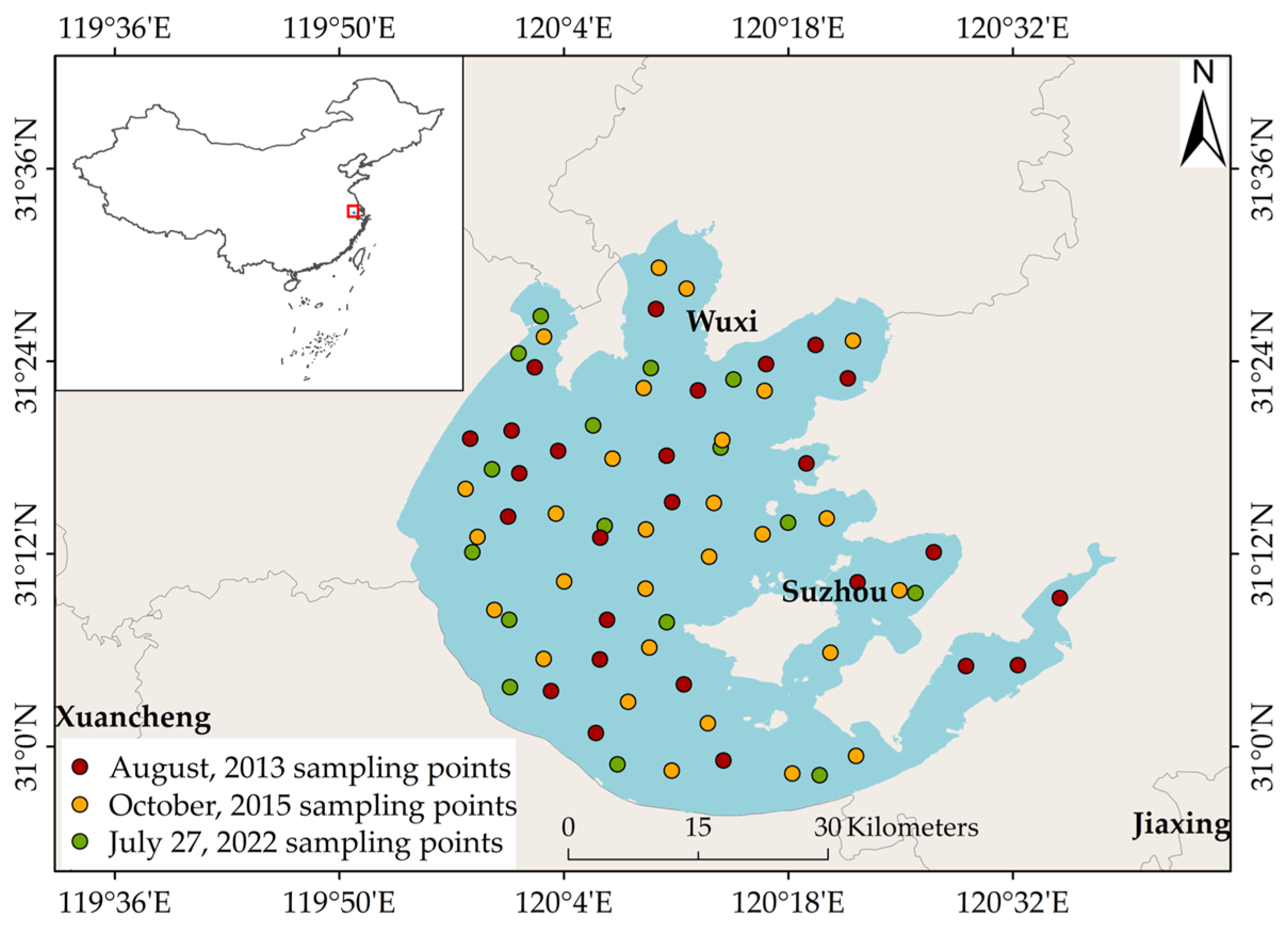
Lake Taihu (30°56′~31°34′N, 119°54′~120°36′E, Figure 1), with a water area of 2338.1 km2, is the third largest freshwater lake in China [29], surrounded by many central cities of the Yangtze River Delta, such as Shanghai, Suzhou, Wuxi, Changzhou, Huzhou, and Jiaxing. It occupies an important position in the process of high-quality development and construction of the surrounding economy and the Yangtze River Delta.

Figure 1.
Study area and measured sample point distribution.
With the economic development and urbanization of the surrounding basin, the water environment of Lake Taihu has been gradually damaged, and the problem of water pollution has become increasingly prominent. Among them, total suspended matter is an important index that intensifies the eutrophication of Lake Taihu and causes water pollution. Due to the shallow water characteristics of Lake Taihu, it is easy to be disturbed by wind and waves, resulting in the suspension of sediment and in perennial turbidity in the lake and significant suspended matter characteristics [30]. The increase in further induces the flow and release of other substances in the lake, promotes the proliferation of algae in the lake, intensifies the eutrophication process of the lake, and ultimately leads to the deterioration of water quality and water pollution. Therefore, monitoring in Lake Taihu is of great significance for improving the water environment and controlling water pollution.
2.2. Field Measurement Data
This study used two measured data sets: the in situ data set from Lake Taihu collected in August 2013 and October 2015 for model construction, and the data collection gathered synchronously with the satellite transit on 27 July 2022, for model verification. In Figure 1, the dots with different colors represented the distribution of the actual sampling points at the three sampling times. The following is a detailed description of the two-part data set:
(1) In August 2013 and October 2015, field data of a total of 54 valid samples were collected in Lake Taihu. The collection process mainly includes the field collection of water spectral data and water samples and the subsequent laboratory analysis of the collected water samples to obtain the concentration data of different components of the water body and the inherent optical data.
A spectrophotometer was used to detect chlorophyll-a concentration (). was determined using the calcination weighing method. When measuring the spectral absorption of chlorophyll-a and suspended matter, the water sample was first filtered by a GF/F glass fiber filter with a diameter of 25 mm and then measured by an ultraviolet/visible dual-beam integrating sphere spectrophotometer [31]. For the measurement of the scattering characteristics of total suspended matter and chlorophyll-a, the original data of the measurement should be corrected and then calculated [32]. CDOM concentration () is usually stated as its absorption coefficient at 440 nm, which was measured by an ultraviolet/visible light spectrophotometer and then converted into an absorption coefficient [33]. The CDOM absorption coefficient is calculated according to the following formula:
where is the absorption coefficient of CDOM. D(λ) is the absorbance of the water sample at wavelength λ, and Lc is the optical range of the cuvette.
(2) To validate the application effect of the inversion model on satellite images, the measured data were determined using water samples collected in Lake Taihu on 27 July 2022 and consisted of 16 sample points. The field sampling date was 27 July 2022, from 7–11 a.m., and the transit of the SDGSAT-1 satellite over Lake Taihu was on 27 July 2022, at 8:51 a.m. Therefore, the synchronization between the field sampling data and the satellite transit time on 27 July 2022 was achieved [34]. The latitude and longitude information of the measured sample points was used to spatially match with the image pixels using geolocalization.
The purpose of water spectral measurement is to obtain water remote sensing reflectance . The water surface spectral data are measured by ASD spectrometer through the above-water method [35]. In the case of avoiding direct solar reflection and ignoring external influences such as solar flares and white caps, the formula for calculating the above-water remote sensing reflectance is as follows:
where is the reflectance of the water body; λ is the wavelength; and , , and are the signal values measured by the spectrometer facing water, sky, and reference plate, respectively. rs is the reflectance of the air–water boundary facing the skylight, which can be 0.022 for a calm water surface, and 0.025 for a wind speed of about 5 m/s, and can be considered between 0.026 and 0.028 for wind speeds of about 10 m/s. is the reflectivity of the reference plate.
2.3. Satellite Remote Sensing Data
This study obtained SDGSAT-1 MII images through the data open system provided by the International Research Center for Big Data for Sustainable Development Goals and selected SDGSAT-1 MII L4 images of Lake Taihu from February 2022 to November 2023 for remote sensing monitoring in Lake Taihu.
Before using remote sensing image data, a series of pretreatment work should be performed, including radiometric calibration, atmospheric correction, water extraction, and so on. The first is radiation calibration, which obtains the calibration gain values of each band of the image from the MII image meta-file. The specific parameters are shown in Table 1. The center wavelength of each channel is the wavelength corresponding to the maximum spectral response of the remote sensor. The formula for converting the observed value DN from satellite load to apparent radiance L is as follows:
where DN is the observed value of the satellite load, L is the apparent radiance, and gain is the gain value of the band.

Table 1.
Band center wavelength and band gain of SDGSAT-1 MII.
As new remote sensing data, the SDGSAT-1 MII image is less researched at home and abroad, and there is no mature atmospheric correction algorithm specially applied to this image. FLAASH model is the most commonly used atmospheric correction model based on the MODTRAN radiative transfer algorithm [36], which applies to different types of sensors, and it can eliminate most of the atmospheric effects effectively. After that, the FLAASH module was used for atmospheric correction of the image to obtain the corrected reflectivity, and then, the output reflectivity image was divided by π to approximate the remote sensing reflectivity of the water [34,37]. Finally, normalized differential water body index (NDWI) was used to extract the mask from Lake Taihu [38].
2.4. Hydrolight Radiation Transfer Simulation
2.4.1. Model Method and Parameter Setting
The Hydrolight model is a tool developed using the radiation transmission theory of water bodies. This software can simulate the light transmission process in a wide range of water environments using the absorption and scattering properties of each component of water bodies. In this paper, the CASE 2 IOPS model of the Hydrolight model is used to simulate the remote sensing reflectance of Lake Taihu. The inherent optical parameters, water quality parameters, environmental conditions, and the spectral range of the absorption model and the scattering model under this model are set as follows:
- Absorption model
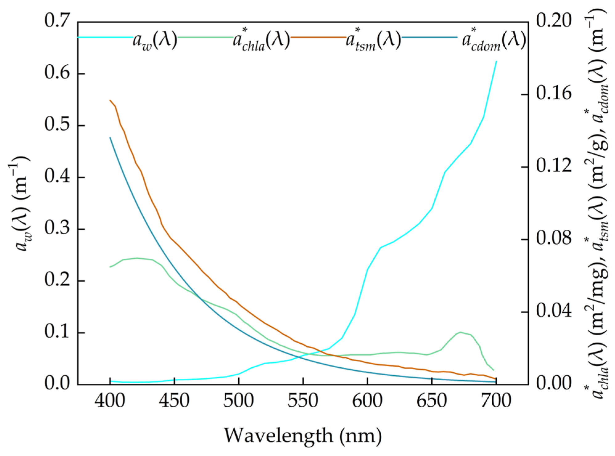
The absorption coefficient a of the water body can be expanded as the sum of all absorption components [39], which is composed of four absorption contributions of pure water, chlorophyll-a, total suspended matter, and CDOM, and each absorption component can be expressed as the product of the inherent optical quantity per unit and the concentration of related components. Therefore, it can be expressed by the following formula:
where a(λ) is the spectral total absorption. , , and represent the absorption coefficient of pure water at wavelength λ, the specific absorption coefficient of chlorophyll-a, and the specific absorption coefficient of total suspended matter, respectively, and the values in the literature [40] are used for , and the mean values of the specific absorption coefficients of all sample points are used for and , and the three-parameter curves are shown in Figure 2. and that used the concentration data of 54 measured sample points were used. could be expressed as the absorption coefficient of CDOM at a wavelength of 440 nm [41], using 54 measured sample points as the input data of . is the specific absorption coefficient of CDOM at wavelength λ, which conforms to the exponential attenuation model with the absorption coefficient of CDOM at a wavelength of 440 nm, and the specific relationship is as follows:
where is the absorption coefficient of CDOM at a wavelength of 440 nm. is the exponential function slope of the CDOM absorption spectrum, and the calculated average is about 0.015. The mean data of obtained for 54 sets of sample points are shown in Figure 2.
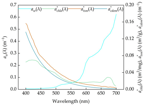
Figure 2.
Absorption spectrum.
- Backscattering model
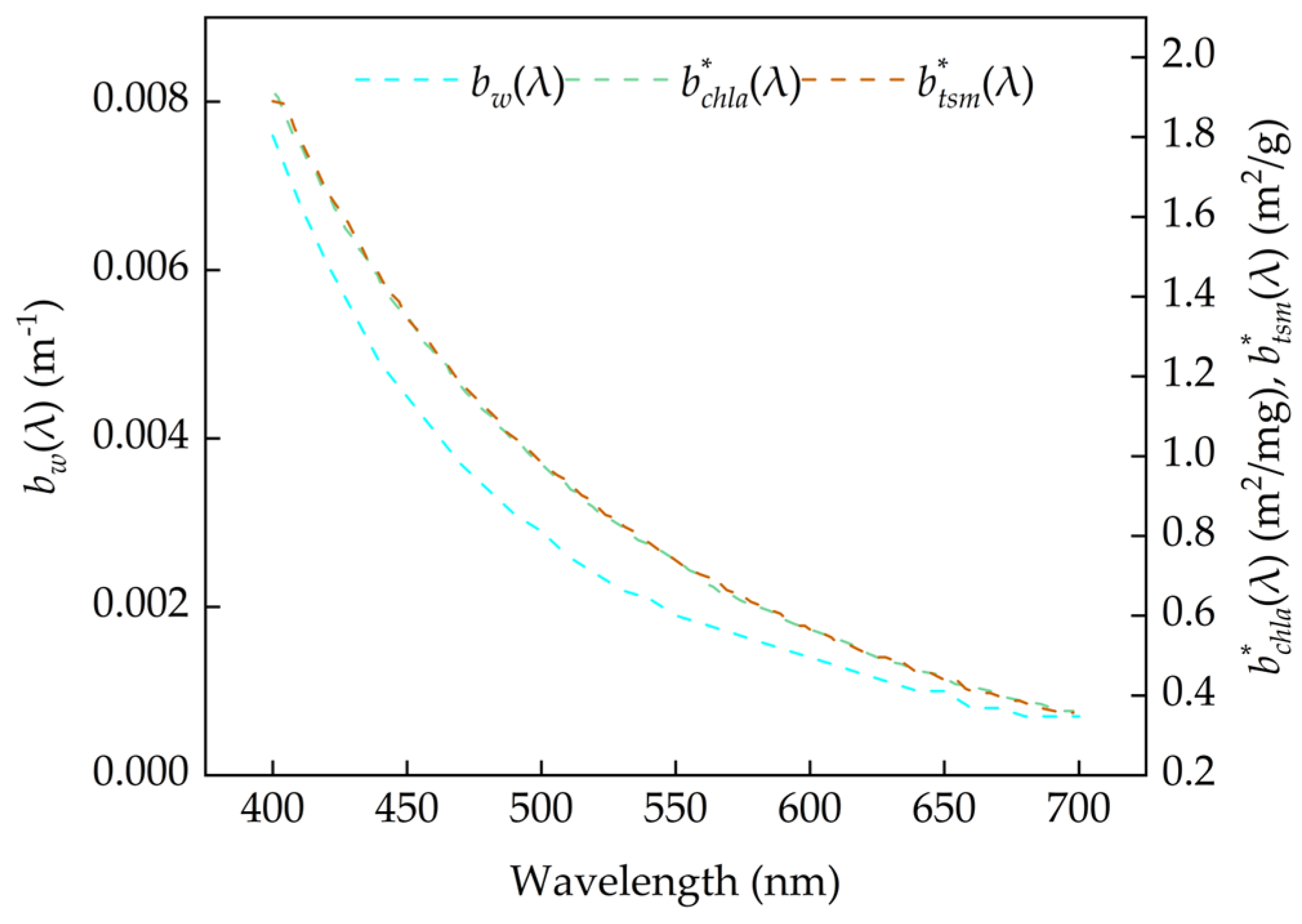
The backscattering coefficient of the water body is composed of the backscattering contributed by pure water, chlorophyll-a, and total suspended matter [26], which can be expressed as follows
where is the backscattering coefficients. , , and are the scattering coefficients of pure water, specific scattering coefficients of chlorophyll-a, and specific scattering coefficients of total suspended matter at wavelength λ. The values of the model in the literature [42] are used for , and the mean values of the specific scattering coefficients of all sample points are used for and . The three-parameter curves are shown in Figure 3. , , and are the backscattering proportions of pure water, chlorophyll-a, and total suspended matter, and the empirical values in reference [43] are set as 0.5, 0.005, and 0.028, respectively.
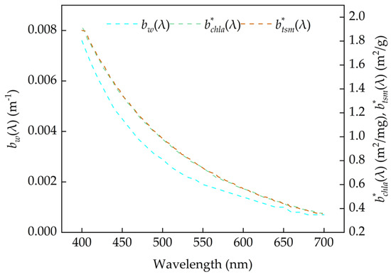
Figure 3.
Scattering spectrum.
- External environmental condition
The RADTRAN model was selected for the sky radiation transmission model, the default values of the weather parameters were adopted, and the refraction index of the water body was set to 1.34.
- The range of the simulated spectrum
The band range of simulated remote sensing reflectance was 400 nm to 800 nm, and the simulation interval was 1 nm.
2.4.2. Influence of Single-Component Concentration Change on Reflectance
Based on the measured concentration ranges of three components, total suspended matter, chlorophyll-a, and CDOM, the Hydrolight model was used to simulate the influence of single-component concentration changes on remote sensing reflectance. In the simulation process, other input parameters remained unchanged except for the concentration of three components. First, a uniform minimum initial concentration was set. was 10 g/m3, was 0.2 mg/m3, and was 0.2 m−1. Subsequently, only the concentration of one component was changed, while the other two components remained unchanged. The change settings of , , and are shown in Table 2, and the remote sensing reflectance simulation data sets under different component concentrations were generated.
Table 2.
Experimental design for characteristic analysis of influence of remote sensing reflectance.
The relative change rate is an indicator used to measure the relative change degree of variables, and its calculation formula is usually the division of the change value by the previous value [44]. Therefore, in order to evaluate the influence degree of total suspended matter, chlorophyll-a, and CDOM on the reflectance under different concentrations, the index of relative change rate is introduced to quantify the relative change in the remote sensing reflectance of water body under different conditions. The specific calculation formula is shown as follows:
where represents the relative change rate, represents the remote sensing reflectance of the water body at wavelength λ after the concentration change, and represents the remote sensing reflectance of the water body at wavelength λ before the concentration change. The high change rate indicates that the remote sensing reflectance is easily affected by the concentration, while the low change rate indicates that the remote sensing reflectance is not easily affected by the concentration.
In order to have a clear understanding of the effect of single-component concentration changes on band reflectance, simulated and were used to analyze the role of single-component concentration changes on the remote sensing reflectance of the center wavelengths of the sensor’s 2nd–6th bands.
2.5. Sensor Channel Convolution and Multi-Band Combination Enhancement
2.5.1. Sensor Channel Convolution
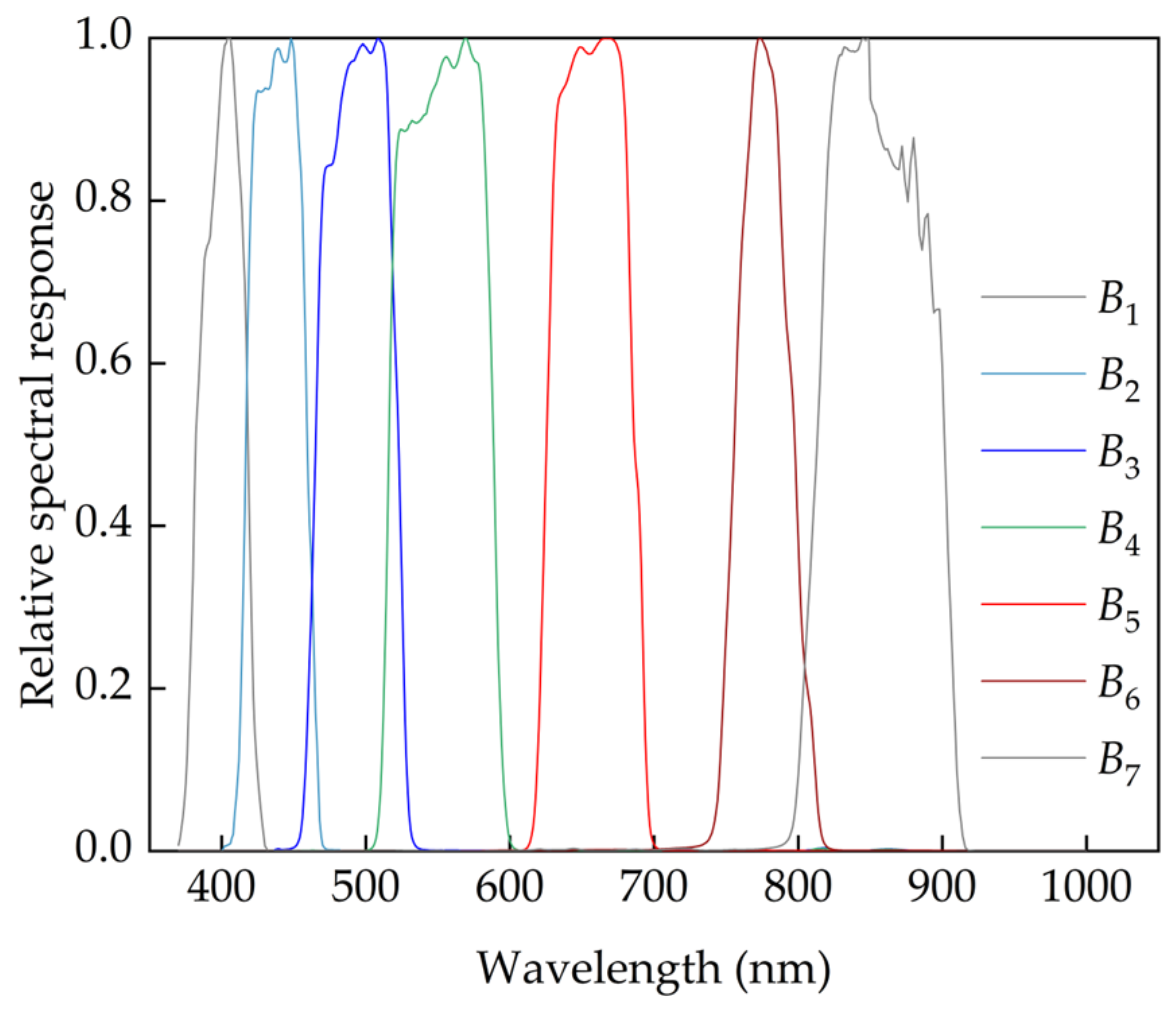
Since the energy actually received by each band of the satellite sensor is the sum of the energy received at each wavelength within the wavelength range of the band, it is necessary to use the spectral response function of the SDGSAT-1 MII sensor (Figure 4) for the convolution of the spectral reflectance simulated by Hydrolight and convert it into the remote sensing reflectance of the corresponding channel of the satellite. The calculation formula is as follows:
where is the equivalent remote sensing reflectance of i channel of the satellite; is the reflectance of the simulated spectrum with an interval of 1 nm; and the spectral range of Hydrolight simulation basically covers the SDGSAT-1 MII channel 2–6. and are wavelengths at both ends of channel i of the satellite; is the spectral response function of the SDGSAT-1 MII sensor.
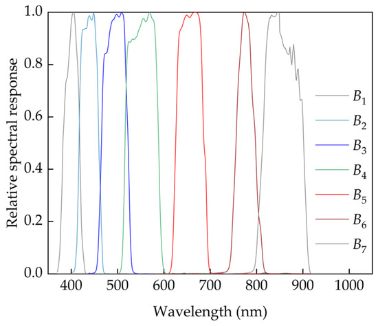
Figure 4.
SDGSAT-1 MII spectral response function.
2.5.2. Multi-Band Combination Enhancement
Compared with the original single-band data, the combination of multi-band mathematical operations helps to eliminate the interference between various bands to a certain extent. Band ratio operation and band difference operation are both effective spectral processing methods, which can highlight the correlation between water quality parameters and water reflectivity [45].
Therefore, ratio reflectance combination and difference reflectance combination were obtained by processing the ratio of and difference in the convolved SDGSAT-1 MII channel reflectance data according to the following formula:
where is the ratio reflectance combination, and is the difference reflectance combination.
2.6. Correlation Analysis
Correlation analysis can quantitatively measure the intensity of linear relationship between variables [46], which provides a basis for the in-depth analysis of the relationship between the component concentration and reflectivity and for subsequent modeling and interpretation. Correlation analysis was conducted between the original band and multi-band combination and the measured , , and in this study.
In the correlation analysis, in addition to the correlation coefficient, a statistic is also obtained, that is, p. The t-test is usually used to determine whether the correlation between the variables is significant, and the level of significance is used to obtain the statistic p to assess whether the correlation between the variables is significant or not. The correlation coefficient, statistic t, and p are calculated by the following formula:
where r is the correlation coefficient, and n is the sample sequence number; N is the total sample size; x represents different original bands and combinations of bands; and y represents , , and . When p > 0.05, there was no significant correlation between the variables. When p < 0.01, it means that the correlation between variables at 0.01 level is significant, and the significance is indicated by **; when p < 0.05, it means that the correlation between variables at the level of 0.05 is significant, and the significance is indicated by *.
2.7. Iterative Inversion Method of Ctsm
2.7.1. Iterative Inversion Method Based on Multiple Linear Regression Analysis
Remote sensing reflectance of the water body is the mixed reflectance of multiple components of the water body, and the mixed reflectance R can be regarded as the linear sum of the contribution of and the contribution of other components concentration, as shown in the following formula:
where R can be the reflectance in the form of different bands and different combinations of bands, viewed as consisting of multiple single-component contributions to reflectance. represents the single-component remote sensing reflectance contributed by , and represents the component remote sensing reflectance contributed by the concentration of other components except .
In order to reduce parameter dependence, the contribution of a single component is regarded as a function of its concentration. For example, the relationship between the single-component reflectance contributed by and is given by the following equation:
where represents the functional relationship between the single-component remote sensing reflectance contributed by and .
The Hydrolight model can simulate the remote sensing reflectance of a single component using a single-component concentration, and the relationship between the remote sensing reflectance of a single component and the concentration of a single component can be obtained. By establishing the multiple linear regression relationship between the mixed remote sensing reflectance and the remote sensing reflectance contributed by a single component, is taken as the unknown in the multiple regression relationship to solve by using different bands or combinations of bands. Therefore, in theory, it is feasible to invert based on multiple linear regression.
The purpose of this study is to reduce the influence of other component concentrations on the inversion of . The most critical thing is to select the appropriate band or band combination as the characteristic band or the characteristic band combination to establish the multiple linear regression relationship between the characteristic band or the characteristic band combination and the single-component remote sensing reflectance, according to the analysis results of the influence of single-component concentration change on the reflectance and the correlation analysis results. This step is a prerequisite for retrieving .
On the premise that the characteristic band or combination of bands is determined as the mixed reflectance, based on the relationship between the concentration of one component and the remote sensing reflectance of one component, and the multiple linear regression relationship between the mixed reflectance and the reflectance of one component, a closed relationship can be formed with as an iterative variable by solving in order to unite the multiple regression model, and an iterative functional relationship can be formed, as shown in the following equation:
where represents the input value of the model, represents the output value of the model, and m represents the calculation times of the model to solve , that is, the number of iterations.
By iterating the function relation, we can derive the next value from the previous value one-by-one and control the cycle process in the form of an infinite approximation solution until the circulation is stopped, when remains unchanged. The final output result represents the inversion result of .
2.7.2. Evaluation Indicators
Three indexes, namely, determination coefficient , root mean square error (RMSE), and mean absolute percentage error (MAPE), are used to evaluate the effect of the inversion model. Their specific calculation formulas are as follows:
where represents the retrieved value of at the hth sample point; represents the measured value of . at the hth sample point. H is the number of sample points.
3. Results
3.1. Validation of Remote Sensing Reflectance Simulations
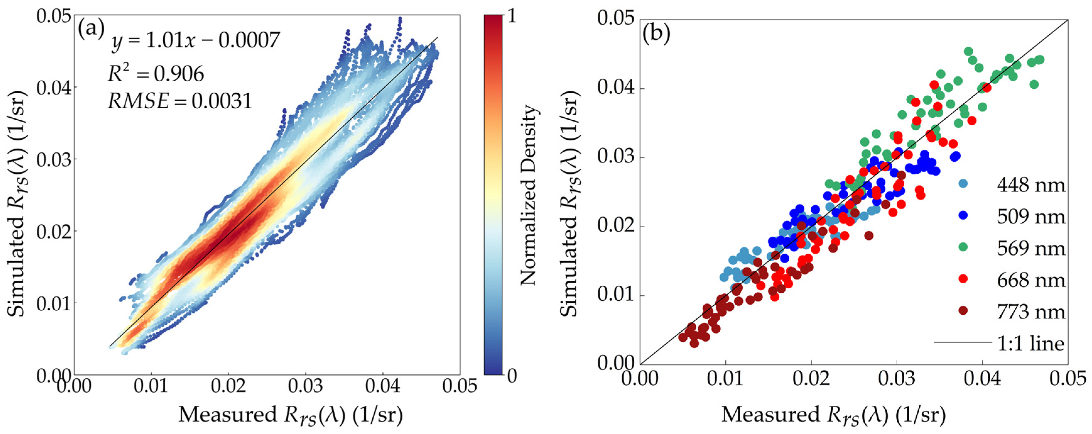
According to the method described in Section 2.4.1, 54 sets of simulated of Lake Taihu in the wavelength range of 400–800 nm were obtained and compared with the measured . The comparison results are shown in Figure A1. The simulated and the measured presented relatively similar curve characteristics, and the spectral trend was relatively consistent. Figure 5a shows the fitting results of the simulated to the measured in the range of 400–800 nm, and there is an obvious linear relationship between the simulated and the measured (R2 = 0.906), and the simulation error is small (RMSE = 0.0031 sr−1). Figure 5b shows the fitting results of the simulated to the measured at the center wavelengths of the satellite bands 2–6, and these scatters are uniformly distributed along the 1:1 line. Error between simulated and measured at the center wavelength of the satellite band are shown in Table 3, with 0.826–0.906 for R2, and RMSE in the range of 0.0025–0.0038 sr−1.

Figure 5.
The simulated is fitted with the measured : (a) in the 400–800 nm and (b) at band center wavelength.
Table 3.
Error between simulated and measured at the center wavelength of the band.
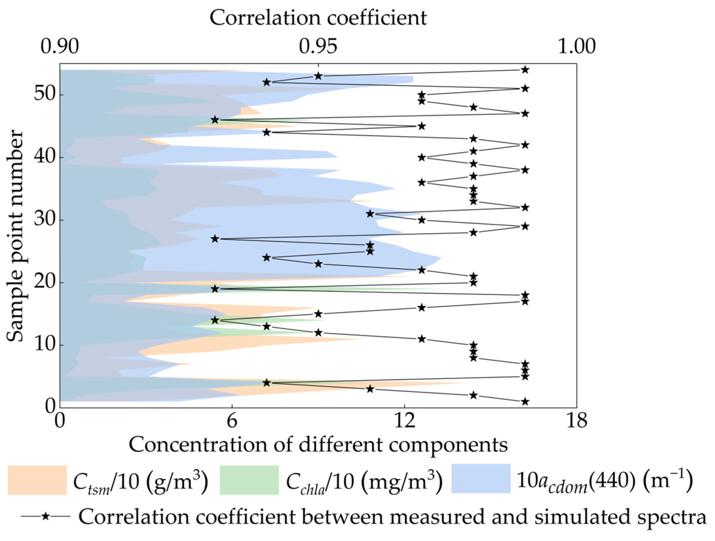
Figure 6 shows the measured data of , , and of 54 sample points, as well as the correlation coefficients between simulated and measured of the 54 sample points. Measured ranged from 15–145 g/m3, measured ranged from 0.27–133 mg/m3, and measured ranged from 0.22–1.33 m−1. The statistical results showed that the correlation coefficients between simulated and measured of the 54 groups of sample points were above 0.93, and the proportion of samples with correlation coefficients greater than 0.95 reached 83.3%.

Figure 6.
The measured concentration data of 54 sample points and the correlation coefficient between the simulated and the measured for 54 sample points.
The above results show that the simulated could be used as reliable basic data for correlation theoretical analysis.
3.2. Analysis of Influence Characteristics of Remote Sensing Reflectance
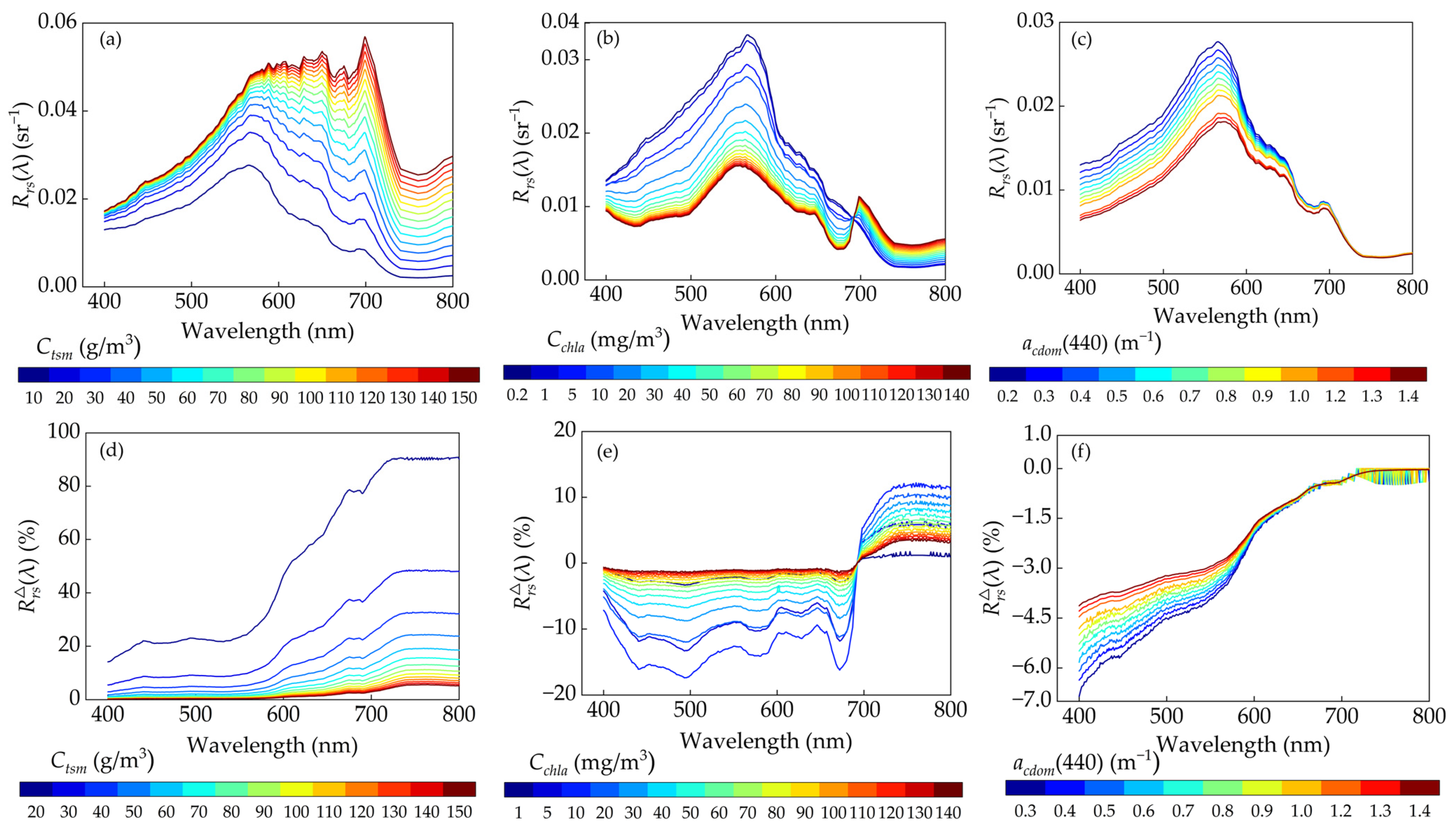
Based on the measured single-component concentration range, an experiment on the effect of single-component concentration changes on was designed, and the simulated data sets were obtained under the conditions that varied from 10 to 150 g/m3, varied from 0.2 to 140 mg/m3, and varied from 0.2 to 1.3 m−1. Using these simulated data sets, the changes in and at different concentrations were analyzed, as well as the effect of a single-component concentration on the center wavelength of the sensor’s bands 2–6, and the results are shown in Figure 7 and Figure 8.
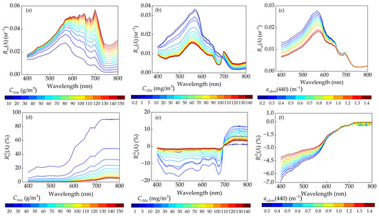
Figure 7.
and under single-component concentration change. (a–c) are obtained under different , , and ; (d–f) are obtained under different , , and .
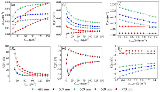
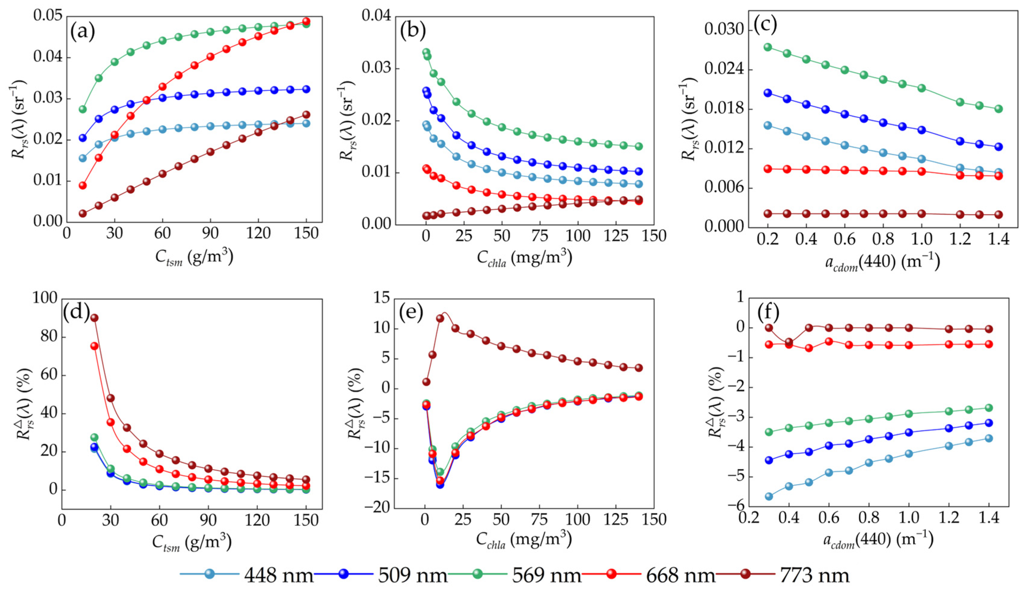
Figure 8.
and under single-component concentration change, λ = 448 nm, 509 nm, 569 nm, 668 nm, and 773 nm. (a–c) are obtained under different , , and ; (d–f) are obtained under different , , and .
In the range of 400–800 nm, and are shown in Figure 7a,d under different . As increased, showed a gradual increase trend, and showed a gradual decrease trend. When was low, was more obvious, and the maximum could cause a 90% relative change. With the increase in concentration, gradually decreased and finally tended to be stable. and are shown in Figure 7b,e under different . Before 700 nm, the increase in led to a decrease in , and decreased. After 700 nm, with the increase in , showed an upward trend, but gradually decreased, resulting in a positive change degree of up to 12%. and under different are shown in Figure 7c,f. The influence of on was weak on the whole. With the increasing wavelength, gradually decreased, and gradually decreased. After 700 nm, is basically no longer affected by the change in .
On the center wavelength of the sensor’s bands 2–6, and at the center wavelength of the five bands are shown in Figure 8a,d under different . With the increase in , at the center wavelength of the five bands showed an increasing trend at the same time, and showed a higher degree of change. and at the center wavelength of the five bands are shown in Figure 8b,e under different . As increased, the trends and extent of changes in at the center wavelengths of the four bands except 773 nm were more consistent. Under different , and at the center wavelength of the five bands are shown in Figure 8c,f. and remained essentially unchanged with an increase in .
3.3. Correlation between Remote Sensing Reflectance and Concentration of Three Components
The results of the correlation analysis between , , and and , , and , respectively, are shown in Figure A2, from which the following can be inferred:
(1) The results of correlation analysis between and the different concentrations are shown in Figure A2a. showed a positive correlation with all five bands, with the strongest significant positive correlation with (r = 0.985 (p < 0.01)); had the strongest correlation with (r = −0.465 (p < 0.01)); showed a negative correlation with all five bands, and with with the strongest correlation (r = −0.649 (p < 0.01)).
(2) In the correlation analysis of with the different concentrations (Figure A2b), 55% of had a significant correlation with above 0.7; 15% of had a significant correlation with above 0.7; and had a correlation above 0.7 with just two ratio combinations of bands.
(3) The results of the correlation analysis between and concentrations are shown in Figure A2c. The number of with significant correlation with higher than 0.7 accounted for 50%; the number of with significant correlation with higher than 0.7 accounted for 40%; and the correlation between and was generally low, among which the strongest correlation was with (r = −0.51 (p < 0.01)).
(4) A comparative analysis of the correlations between concentrations and different bands and combinations of bands showed that three bands (, , ), as well as six combinations of ratios (, , , , , ) and eight combinations of differences (, , , , , , , ), were significantly correlated with the three component concentrations at the same time, indicating that it is inappropriate to rely on the bands and combinations of bands related to alone for the inversion of , and it is not possible to avoid the effects of the other components.
(5) With a further comprehensive comparison of the correlation characteristics of the three component concentrations, as well as by combining the results of the characterization of the effects of the three component concentrations on reflectance in Section 3.2, it can be concluded that has a weak effect on reflectance, while there is a more obvious correlation between and and remote sensing reflectance, and the two are the dominant factors affecting remote sensing reflectance.
Based on the above conclusions, in order to eliminate the other component contributions from the remote sensing reflectance and then invert independently, the basic idea of constructing model in this study includes the following:
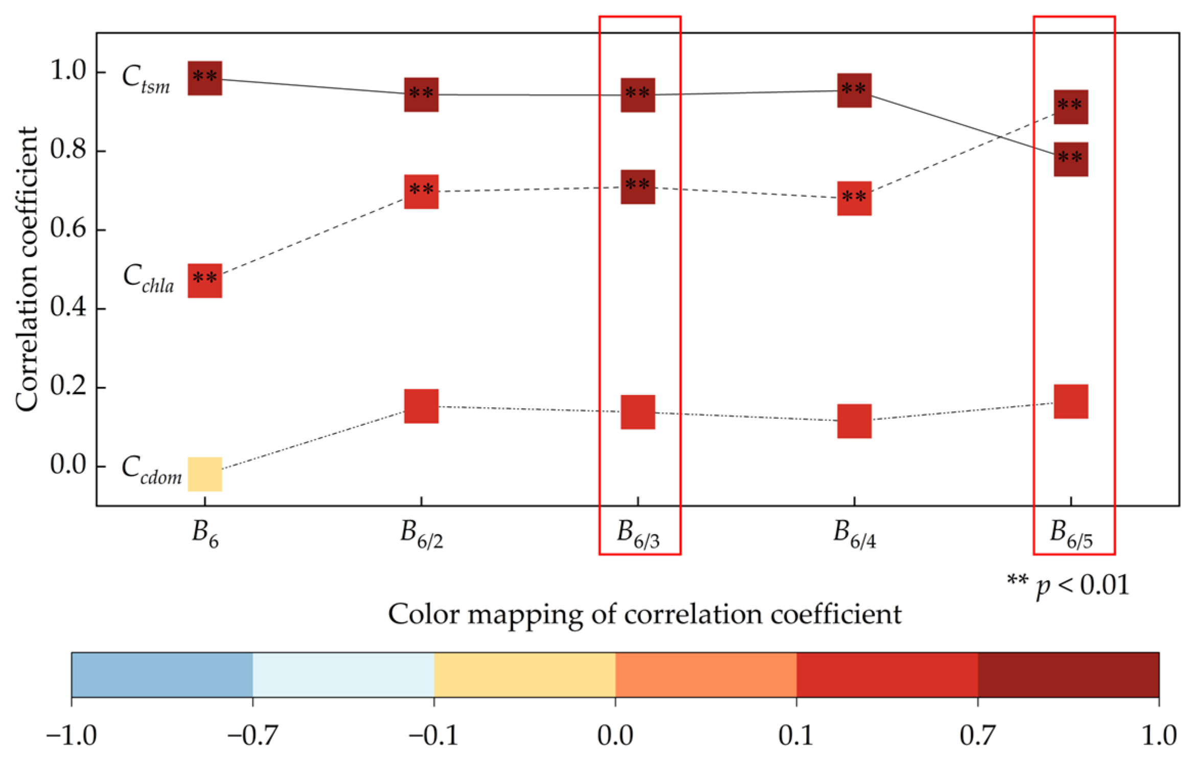
(1) Firstly, the band or combination of bands that did not correlate with but showed a correlation with and were selected, and the results are shown in Figure 9, which were regarded as the combined contribution of the two components of and , so that the influence of was no longer taken into account.
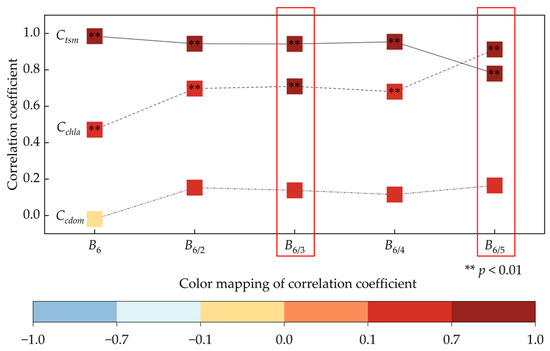
Figure 9.
Bands and band combinations that are not related to but to and .
(2) Next, the bands or band combinations that showed a significantly strong correlation (r > 0.70 (p < 0.01)) with both and were selected as factors, and multiple linear regression and iterative resolution methods were used to remove the signals of from the remote sensing reflectance, and thus extract .
Finally, and were identified as two band combination characterization factors for subsequent multiple linear regression and iterative parsing studies.
3.4. Multivariate Iterative Inversion Model Construction and Evaluation
3.4.1. Multivariate Iterative Inversion Model Construction
- Reflectance simulation of single-component contribution
and were regarded as the mixed reflectance of both and . In order to accurately invert , it is necessary to simulate the contribution of and , respectively, followed by contribution elimination through multivariate iteration.
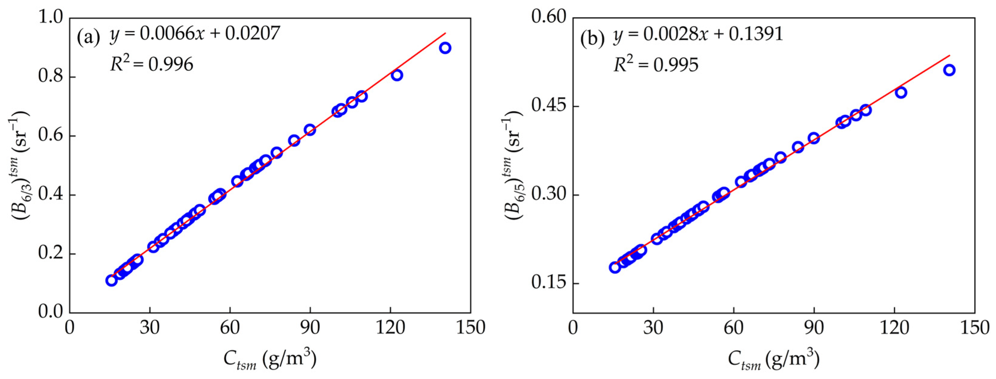
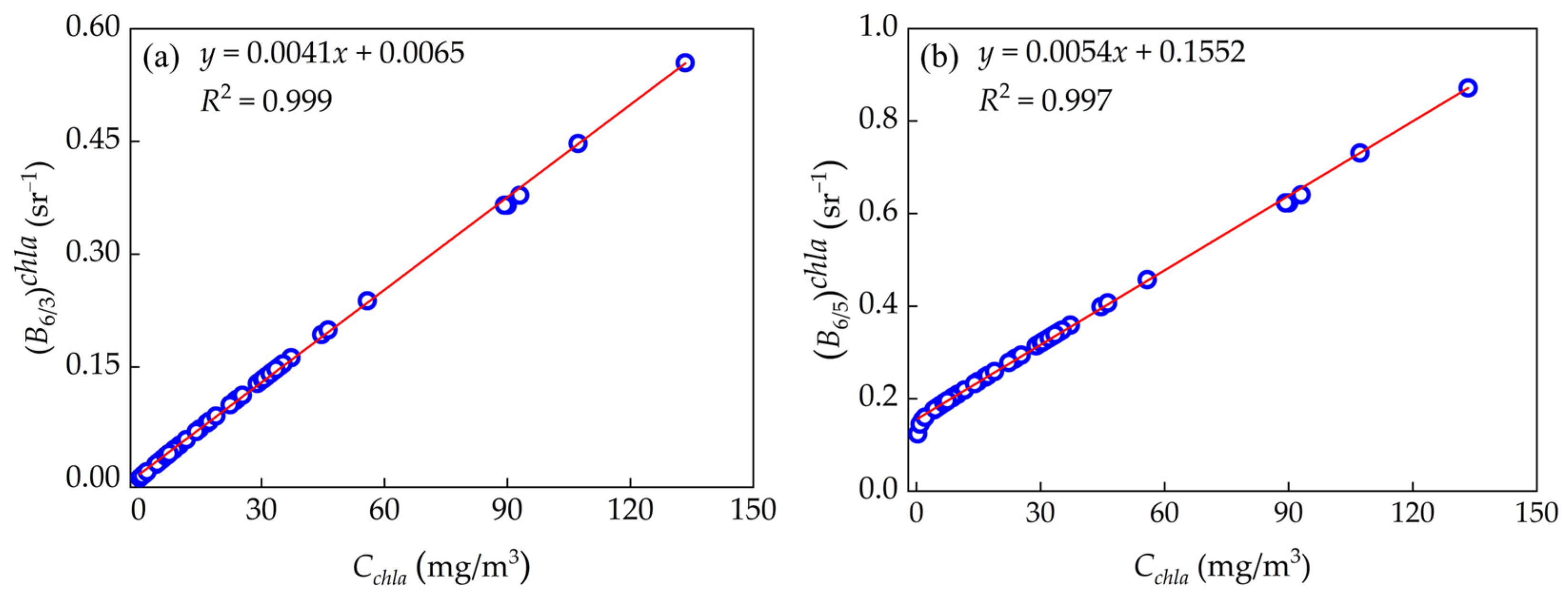
Based on the measured concentration data, Hydrolight was used to simulate the single-component contributions to obtain the single-component reflectance of the contribution from and the single-component reflectance of the contribution from (Figure 10 and Figure 11), respectively, and the relationship that exists between the component concentrations and the respective contributions to the reflectance is shown in the following equations:
where and are single-component reflectances contributed by , and and are single-component reflectances contributed by .
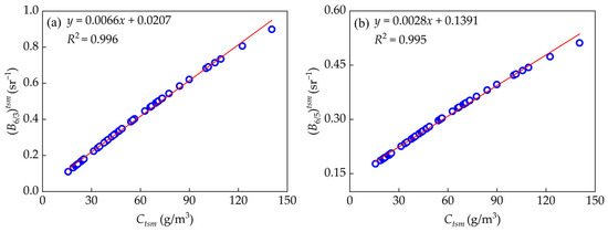
Figure 10.
The relationship between and the single-component remote sensing reflectance contributed by : (a) and (b) .
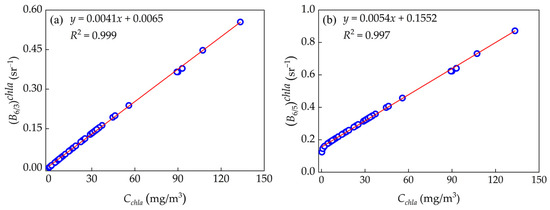
Figure 11.
The relationship between and the single-component remote sensing reflectance contributed by : (a) and (b) .
The results showed that there was a significant linear relationship between the component concentrations and their respective contributions to remote sensing reflectance, with R2 being greater than 0.99 in all cases.
- Multiple linear regression analysis
According to Equation (14) in Section 2.7.1, and are equivalent to the mixed reflectance R, can be regarded as the linear sum of the reflectance contributed by each of and , i.e., a linear combination of and , and can be thought of as the linear sum of the reflectance contributed by each of and , i.e., a linear combination of and . Multiple linear regression analysis between the mixed reflectance R and the single-component reflectance using Equation (14). The objective of this study is to solve by combining Equation (15) from Section 2.7.1 with a multiple linear regression analysis, and therefore, a single-component-contributing reflectance is used as the dependent variable in performing the multiple linear regression, and a characteristic band combination and another single component contributing reflectance are used as independent variables.
Considering the correlation between and (r = 0.942, p < 0.01, Figure 9) was higher than that with (r = 0.709, p < 0.01, Figure 9), a multiple regression was established with as the dependent variable, and and as the two independent variables. Meanwhile, correlation with (r = 0.912, p < 0.01, Figure 9) was greater than the correlation with (r = 0.779, p < 0.01, Figure 9), and therefore, was used as the dependent variable and a multiple regression relationship was established with and as the two independent variables.
and were obtained by ratio combination based on satellite channel data after the convolution of 54 sets of simulated spectra, and simulated from of the 54 sample sites (Figure 10), and and simulated from of the 54 sample sites (Figure 11), which correspond to the decomposition of the component contributions to and .
Based on the above analysis and on the principle of Ordinary Least Squares (OLSs), the multivariate linear regression equations were established by Python, and the two regression equations obtained were expressed as follows.
The corresponding R2 of the two regression equations were 0.977 and 0.991, indicating that the models were well fitted. The residual is the difference between the predicted value of the dependent variable and the cause variable obtained after multiple linear regression. The residuals of the two models were located between −0.045–0.059 sr−1 and −0.015–0.034 sr−1, respectively, with smaller residual values, which indicated that the multiple linear regression model was able to predict the dependent variable more accurately.
- Construction of the iterative inversion model
Based on the multiple linear regression analysis, the two multiple regression models (Equations (24) and (25)) were combined with the relationship between the concentration and the respective contributing reflectance, thus forming a complete closed iterative inversion model, which is shown in the following equation:
The input parameter settings of the iterative inversion model in different application scenarios are shown in Table 4. In the iterative inversion model, , , and were used as the input parameters of the model, and this iterative functional relationship was convergent and able to calculate iteratively. When the successive output values gradually converged to be equal, i.e., the difference between the output value and the input value gradually tended to be zero, which indicated that the algorithm was approaching the solution until the output value was kept unchanged, the iterative process was stopped, and the last guessed value was used as the final inversion result of .
Table 4.
Model input parameter setting.
3.4.2. Analysis of the Initial Value Setting of Ctsm(0)
Firstly, the model was applied to the modeling data, and the calculation method was adopted by numerical iteration one-by-one. The input data of the model included , , and . And was initialized to 0 as the output value. In the iterative process, both and were updated automatically according to the iterative formula (Equation (26)).
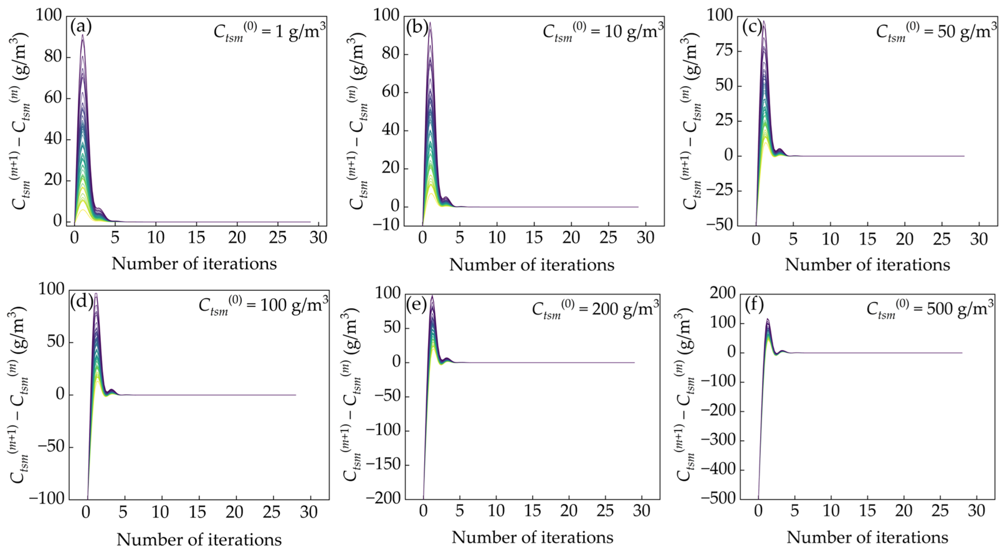
In order to analyze the impact of the initial value on the model, the of each group was set as 1 g/m3, 10 g/m3, 50 g/m3, 100 g/m3, 200 g/m3, and 500 g/m3, respectively. Figure 12 shows the change in the difference between the 54 sets of output values and input values during iteration, using 54 groups of curves of different colors. Under different values of , the difference between the output value and the input value decreased gradually with the iteration. When the output value and the input value were consistent, the iteration process stopped, and each group of values was iterated 29 times. The model achieved the same output results under different settings, and the number and time of calculation did not change with the specified initial value of . The results showed that the iterative inversion model had no dependence on the initial value of , and the initial value of could be set arbitrarily.
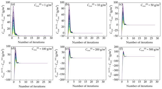
Figure 12.
The change in the difference between each set of output value and input value during iteration.: (a) = 1 g/m3; (b) = 10 g/m3; (c) = 50 g/m3; (d) = 100 g/m3; (e) = 200 g/m3; and (f) = 500 g/m3.
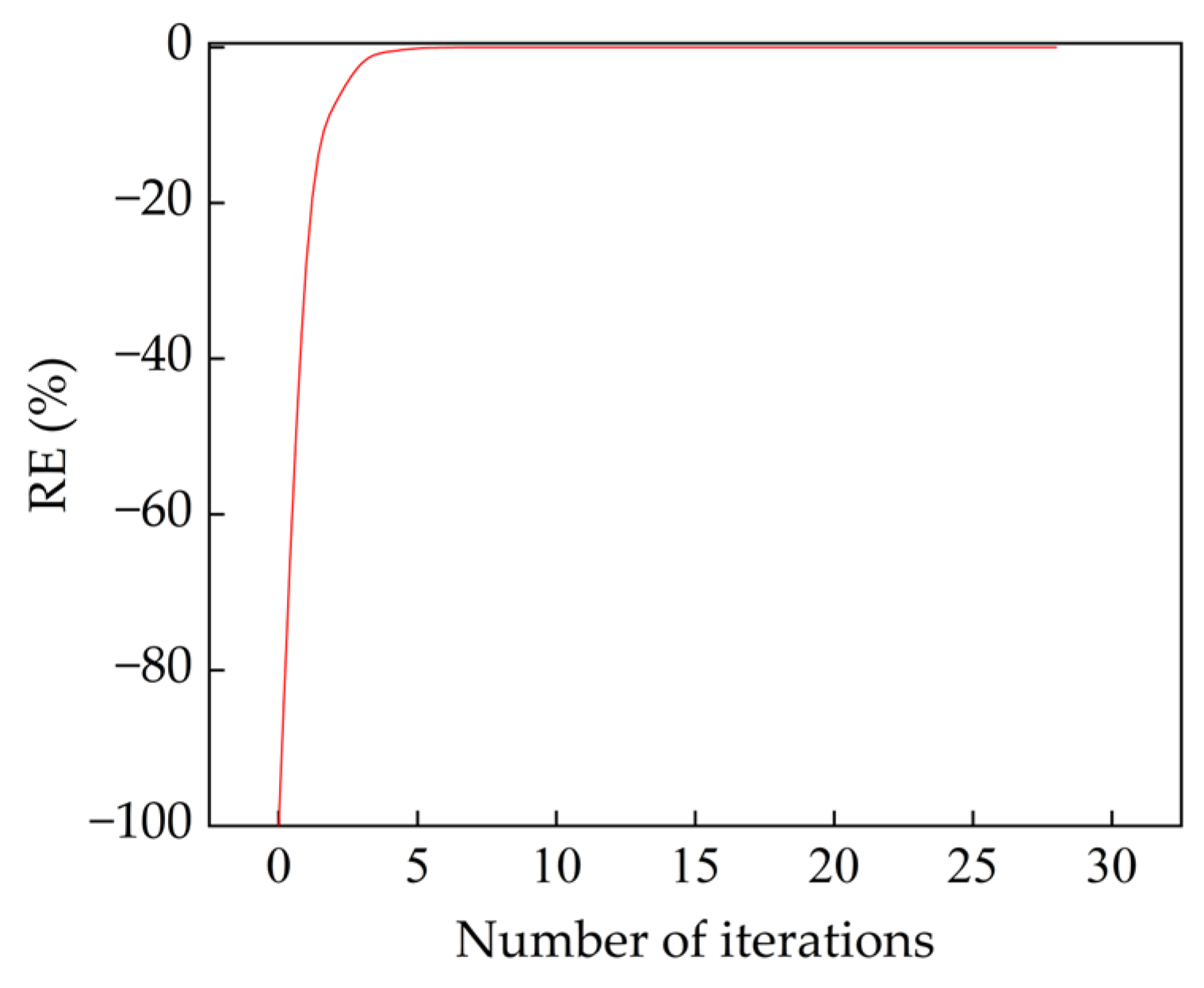
In addition, the relative error (RE) was used to quantify the convergence accuracy in the iterative process, which was defined as the difference between the output value of the current iteration and the final output value divided by the final output value, and was expressed as a percentage. When = 1 g/m3, RE changes in the iteration process are shown in Figure 13. With the progress of iteration, RE decreased gradually. When the number of iterations was five, RE reached −0.15%. When the number of iterations was 10, RE decreased to −0.0002%. When the number of iterations reached 29, RE dropped to 0, indicating that the model had successfully converged to the final solution and reached a stable output state.
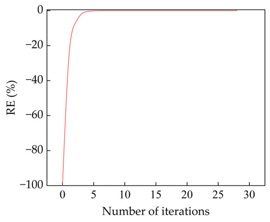
Figure 13.
The change in RE in the process of iterative convergence.
By analyzing the measured and the retrieved of the iterative inversion model, the accuracy of the iterative inversion model was evaluated (Figure 14). There was a highly significant linear relationship between the measured value of and the inversion value, R2 was 0.97, and the difference between the two was small, and the obtained RMSE and MAPE were 4.89 g/m3 and 11.48%, respectively, indicating that the model had good accuracy.
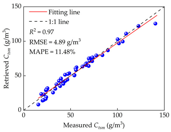
Figure 14.
The measured are fitted to the retrieved of the iterative model.
3.4.3. Valuation of Ctsm Estimation Methods for SDGSAT-1 MII Image
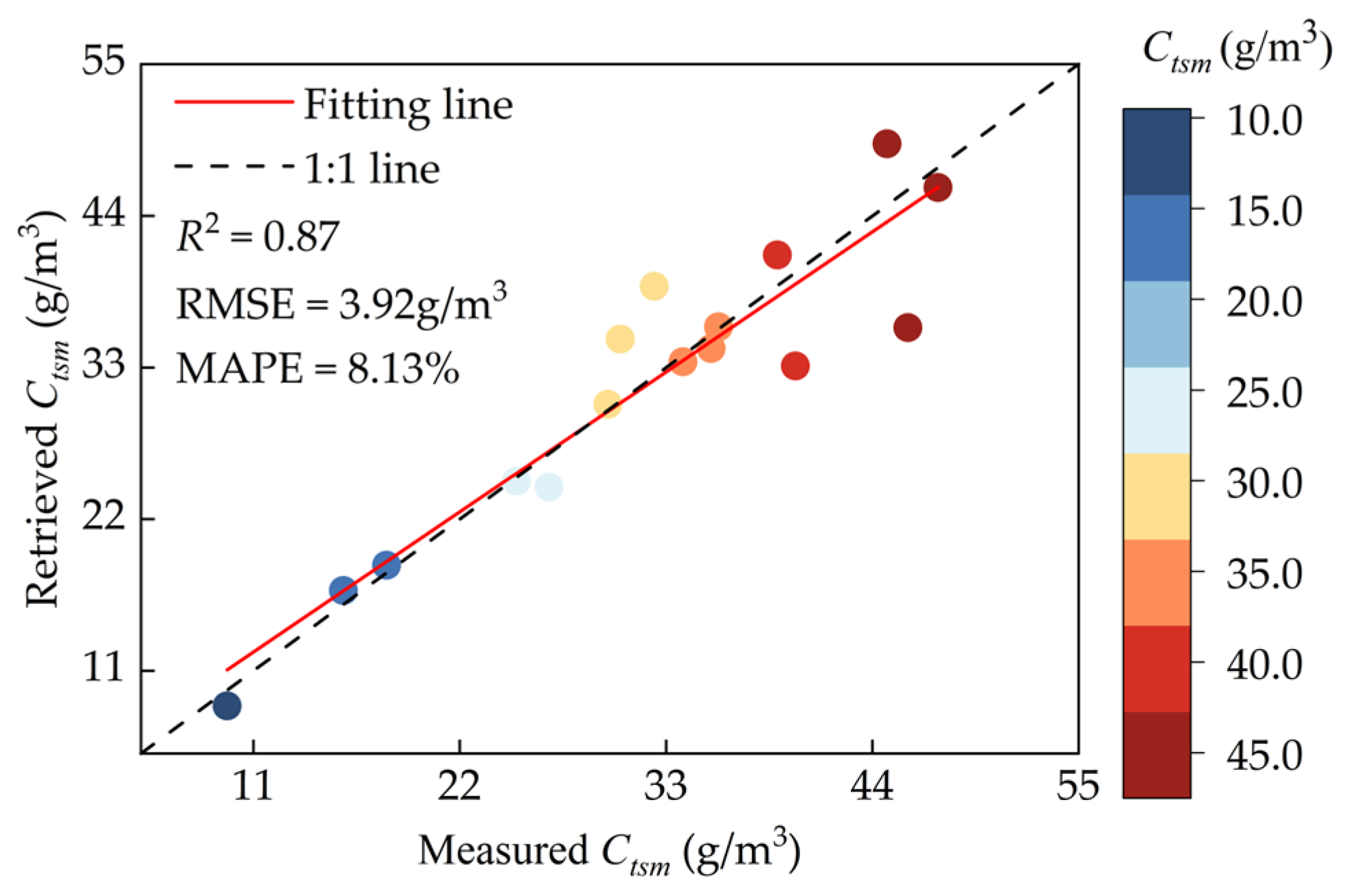
The iterative inversion model constructed in this paper was applied to the pre-processed SDGSAT-1 MII image of 27 July 2022, and verified by using the ground and satellite synchronization data by adopting the pixel-by-pixel iterative calculation method. The comparison results between the measured and the retrieved are shown in Figure 15. They were uniformly distributed along the 1:1 line, and their R2 was 0.87, showing extremely high linear correlation and consistency, and the error level was relatively low, with a RMSE of 3.92 g/m3 and a MAPE of 8.13%. The verification results showed that the iterative inversion model proposed in this paper showed a good application effect and good application accuracy on the SDGSAT-1 MII image.
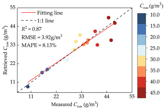
Figure 15.
The measured is fitted to the retrieved from the SDGSAT-1 MII image, based on the iterative model.
4. Discussion
4.1. Comparison between Different Characteristic Band Combinations
The aim of this paper is to eliminate the other component contributions from the reflectance and thus invert the suspension concentration independently, and based on the results of the analyses in Section 3.2 and Section 3.3, it is concluded that , , , , and do not correlate with but rather correlate with and . Thus, it is possible to consider , , , , and as and as the combined contribution of the two components (Figure 9); thus, the effect of is no longer considered. Furthermore, to remove the signal of present in reflectance, and , which showed significant strong correlation (r > 0.70 (p < 0.01)) with both and , were selected as factors for multiple linear regression and iterative resolution.
In order to evaluate the advantage of constructing an iterative inversion model for the inversion of using and as characteristic band combinations, from the band and band combinations that do not correlate with but correlate with and (Figure 9), other band and band combinations were selected as new characteristic band combinations to construct new iterative inversion models for comparative studies.
Considering that only had a greater correlation with than , was left unchanged. Among the bands and band combinations with higher correlation with suspended matter concentration than , the correlations of , , , and with were all greater than 0.9, but there was a difference in the correlation with , where the correlation of was greater than 0.7 and the correlation of with was only 0.471, and the correlations of , , and were greater than 0.65, and , and were used as the characteristic band combinations for constructing the iterative inversion model together with , respectively.
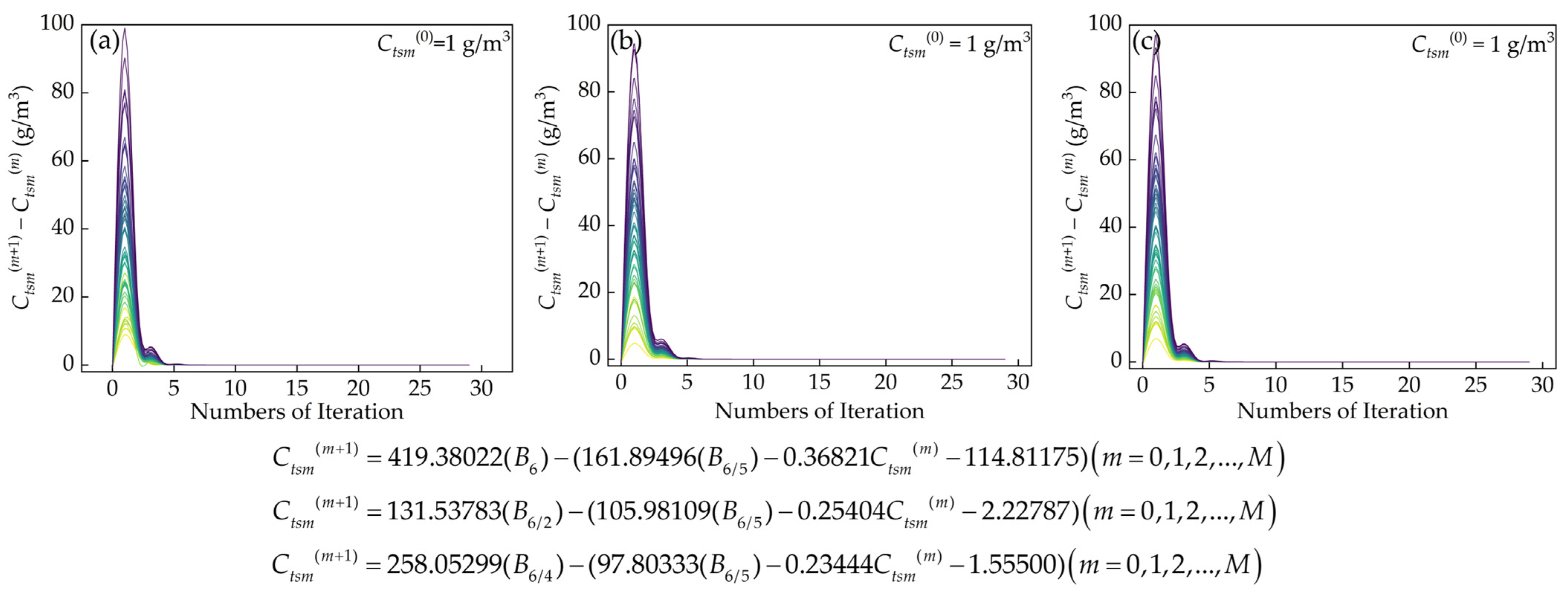
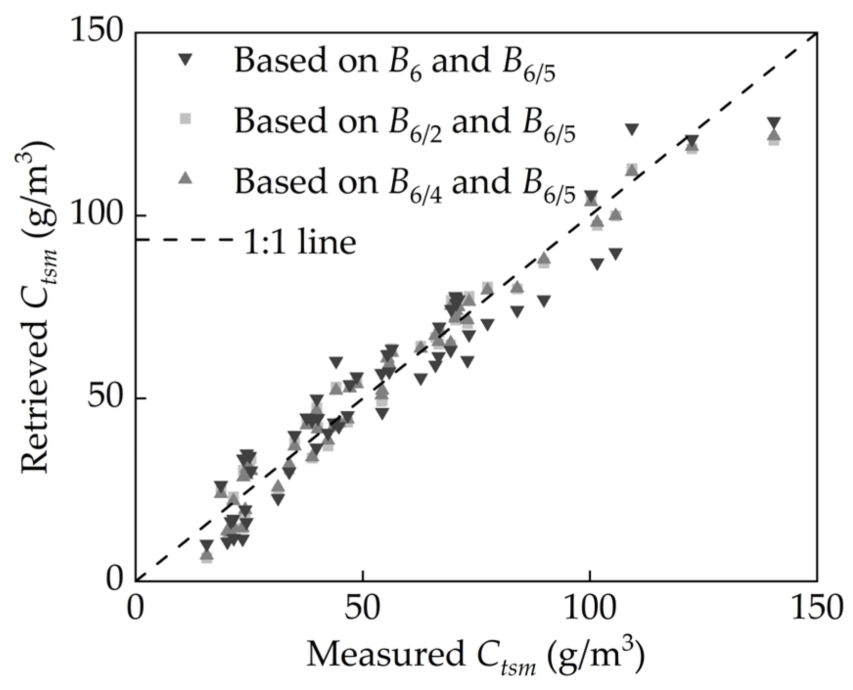
Three iterative inversion models based on and , and , and and were formed by repeating the previous processing process. The iterative inversion of applied to the modeling data are shown in Figure 16 by the three newly constructed iterative inversion models, the 54 sets of curves with different colors represent the changes in the difference between the 54 sets of output values and input values during the iteration process. When models were applied to the modeled data, was uniformly set as 1 g/m3, and the three iterative inversion models carried out 29 iterations for each set of values. Figure 17 shows the fitting of the three iterative inversion models between the final output iterative inversion values and the measured values of each group, and the results are relatively close. Subsequently, the three newly constructed iterative inversion models were applied to the pre-processed SDGSAT-1 MII image of 27 July 2022, and verified using the ground and satellite synchronization data. The results are shown in Figure 18, where a few points deviate from the 1:1 line to a large extent.
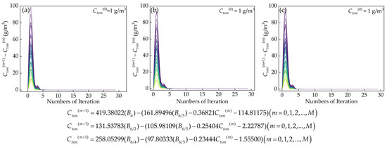
Figure 16.
Change in the difference between the output value and the input value during the iteration process: (a) based on and ; (b) based on and ; and (c) based on and .

Figure 17.
Fitting of measured and retrieved when models are applied to the modeled data.
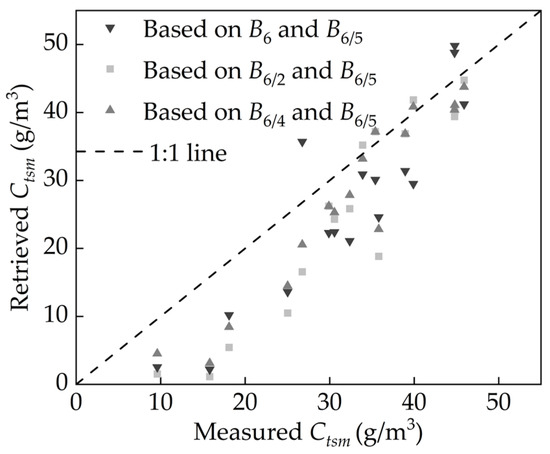
Figure 18.
Fitting of measured and retrieved when models are applied to the SDGSAT-1 MII image of 27 July 2022.
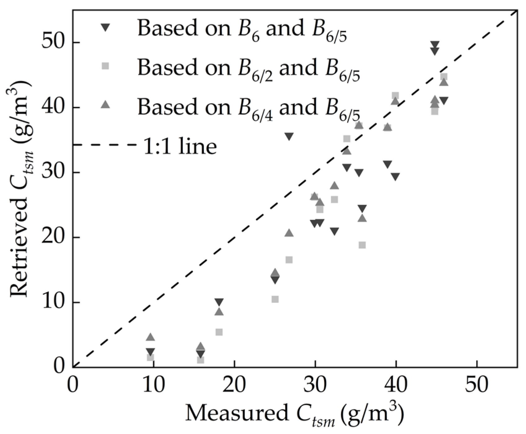
By comparing the modeling errors of the four iterative inversion models and the errors applied to the SDGSAT-1 MII image (Table 5), the comparison results showed that the modeling accuracy and application effect of the three new iterative inversion models were not as good as the iterative inversion models based on and , which indicated the iterative inversion model based on and showed higher accuracy and a better ability of retrieving .
Table 5.
Error statistics for four iterative inversion models.
4.2. Comparison with Other Inversion Models
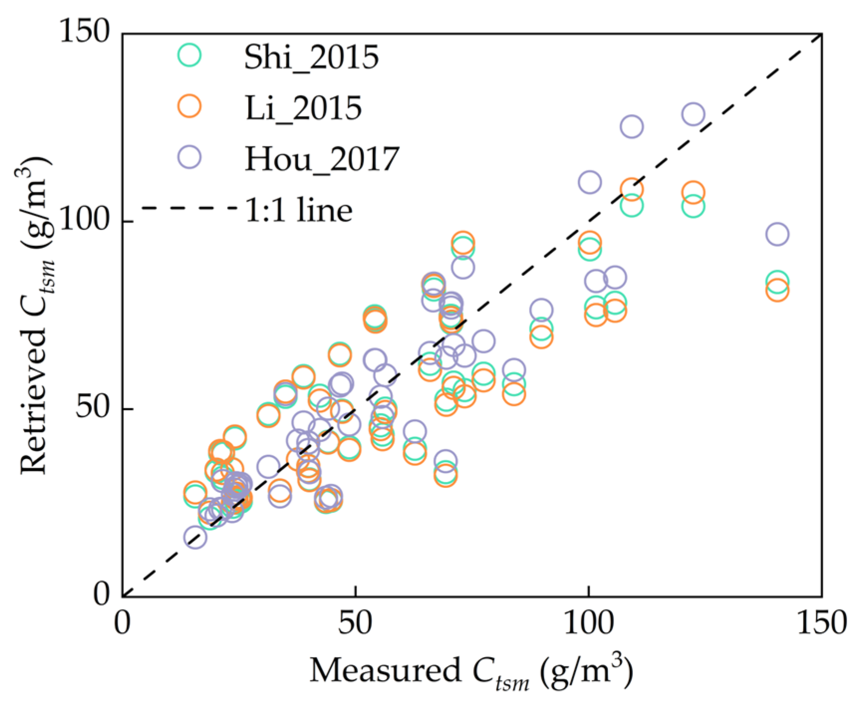
Referring to the inversion models of proposed by other researchers in recent years, the measured data used in this study were applied to the corresponding models to obtain the adapted models (Table 6), which were applied for the estimation of in Lake Taihu, and the results of the fit between measured and retrieved are shown in Figure 19. Among these adapted models, the Hou_2017 model [18] had the highest modeled accuracy in Lake Taihu, but its error was still large compared with the iterative inversion model proposed in this paper when models were applied to the modeled data.
Table 6.
The model and accuracy of inversion model after adaption.
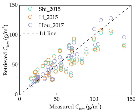
Figure 19.
Fitting of measured and retrieved when the adapted models are applied to the modeled data [18,47,48].
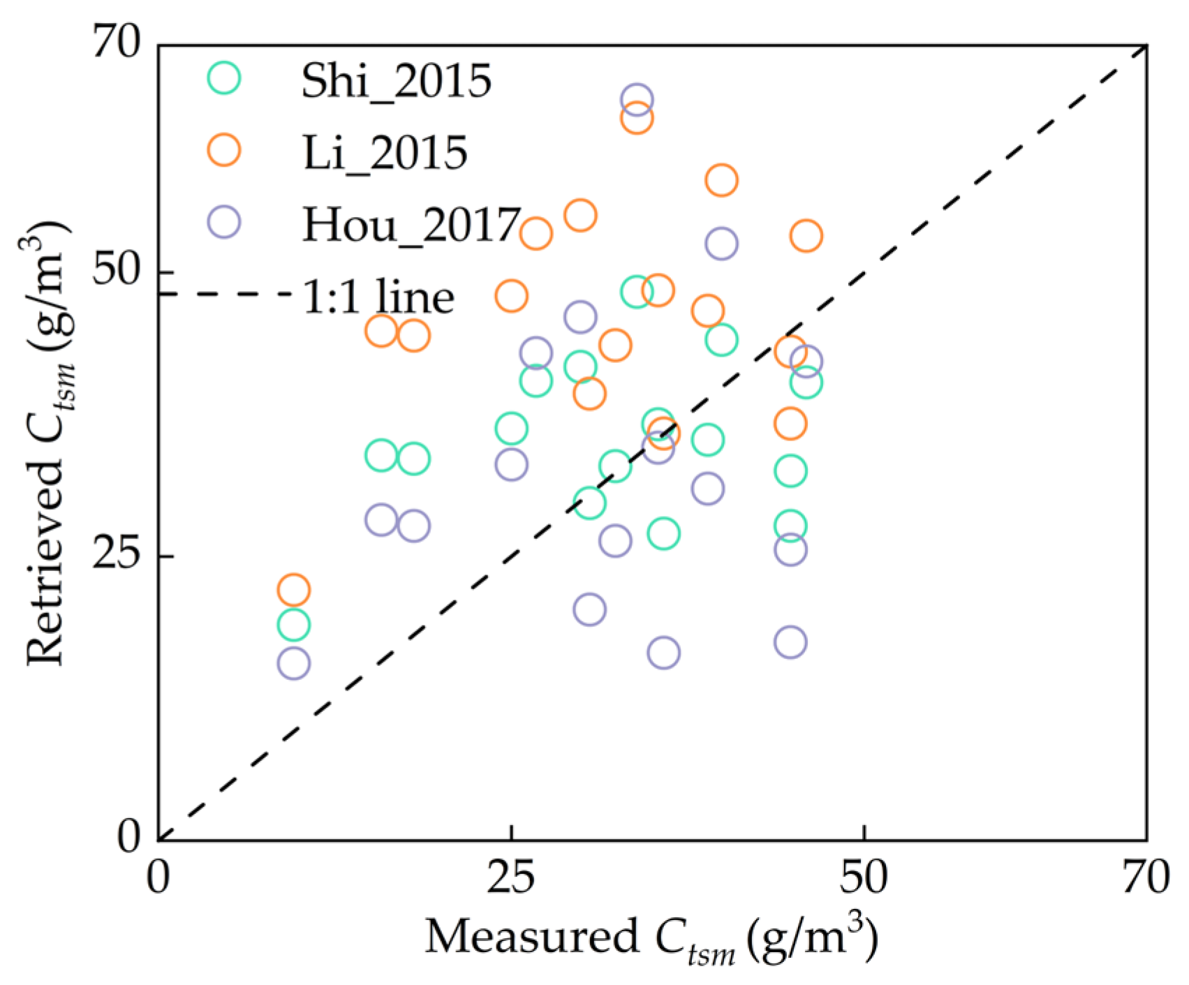
These models were applied to the pre-processed SDGSAT-1 MII image of 27 July 2022, using as , and as and , and validating them using the synchronized ground-satellite data (Figure 20). The RMSE and MAPE between measured and inverted are listed in Table 7. The results showed that the Shi_2015 model [47] had the smallest error in the imagery among the adapted models. However, all of these adapted models performed poorly in terms of imagery applicability when compared to the iterative inversion model proposed in this paper.
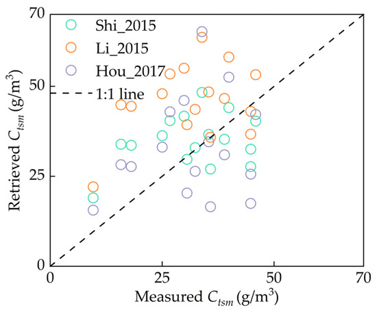
Figure 20.
Fitting of measured and retrieved when the adapted models are applied to the SDGSAT-1 MII image of 27 July 2022 [18,47,48].
Table 7.
Error statistics when models are applied to the SDGSAT-1 MII image of 27 July 2022.
4.3. Temporal and Spatial Distribution Characteristics of Ctsm in Lake Taihu
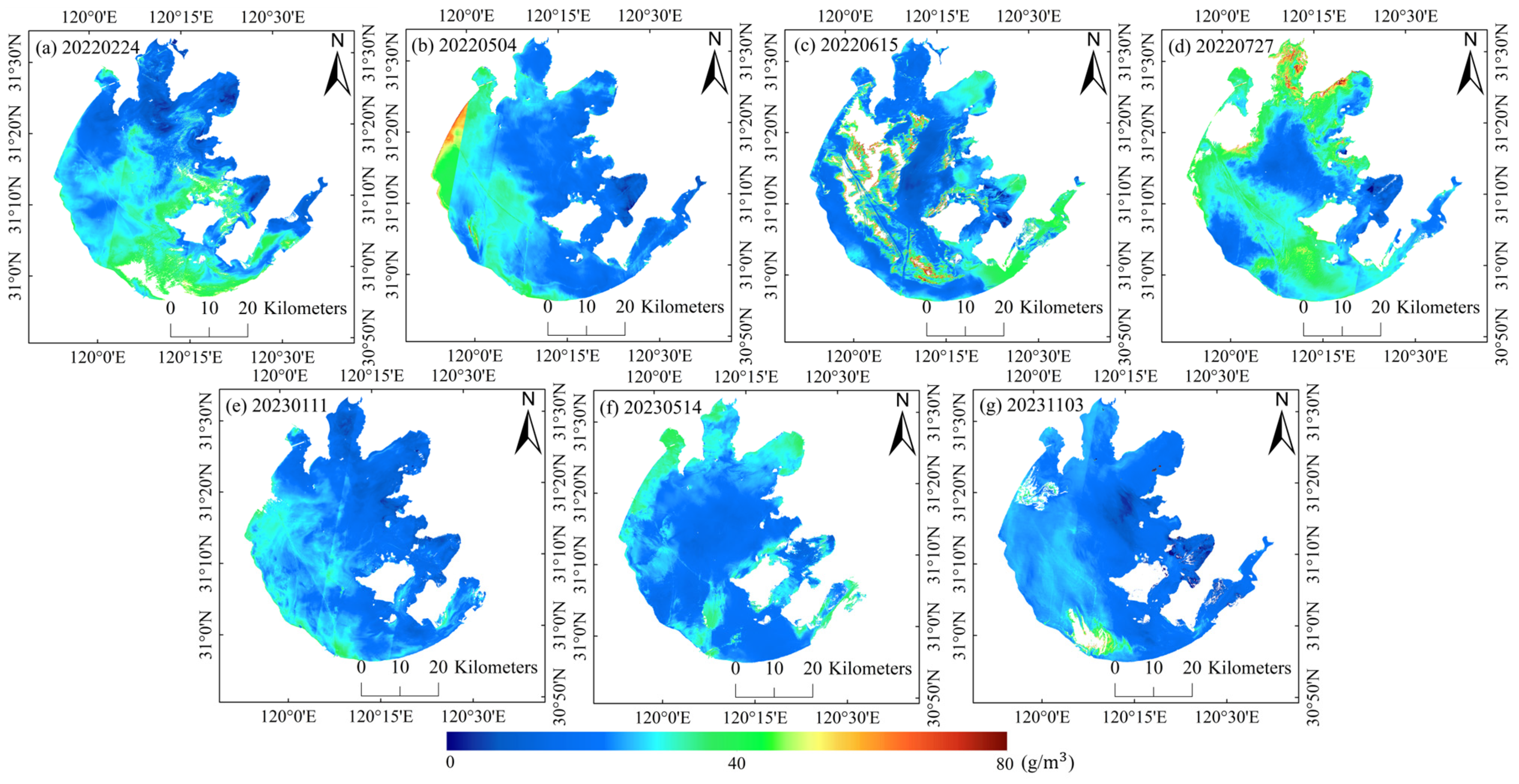
The iterative inversion model based on and is applied to the SDGSAT-1 MII images available in 2022–2023 for the observation of in Lake Taihu, and the spatial distribution results are shown in Figure 21. There were some seasonal differences in the spatial distribution of in Lake Taihu, with low concentrations mainly concentrated in the center of the lake. In May, June, July, and November, in the center of the lake was low and lower than that in the surrounding waters. The reason for this was that the vegetation growing in the water could effectively prevent suspended sediment from being resuspended, thus slowing down the increase in ; in January and February, the aquatic vegetation was in the sinking stage, coupled with the frequent monsoon winds, and the suspended sediment was resuspended again under the action of the wind; thus, in this period showed a phenomenon of accumulation in the central area of the lake.

Figure 21.
Spatial distribution of in Lake Taihu, 2022–2023.
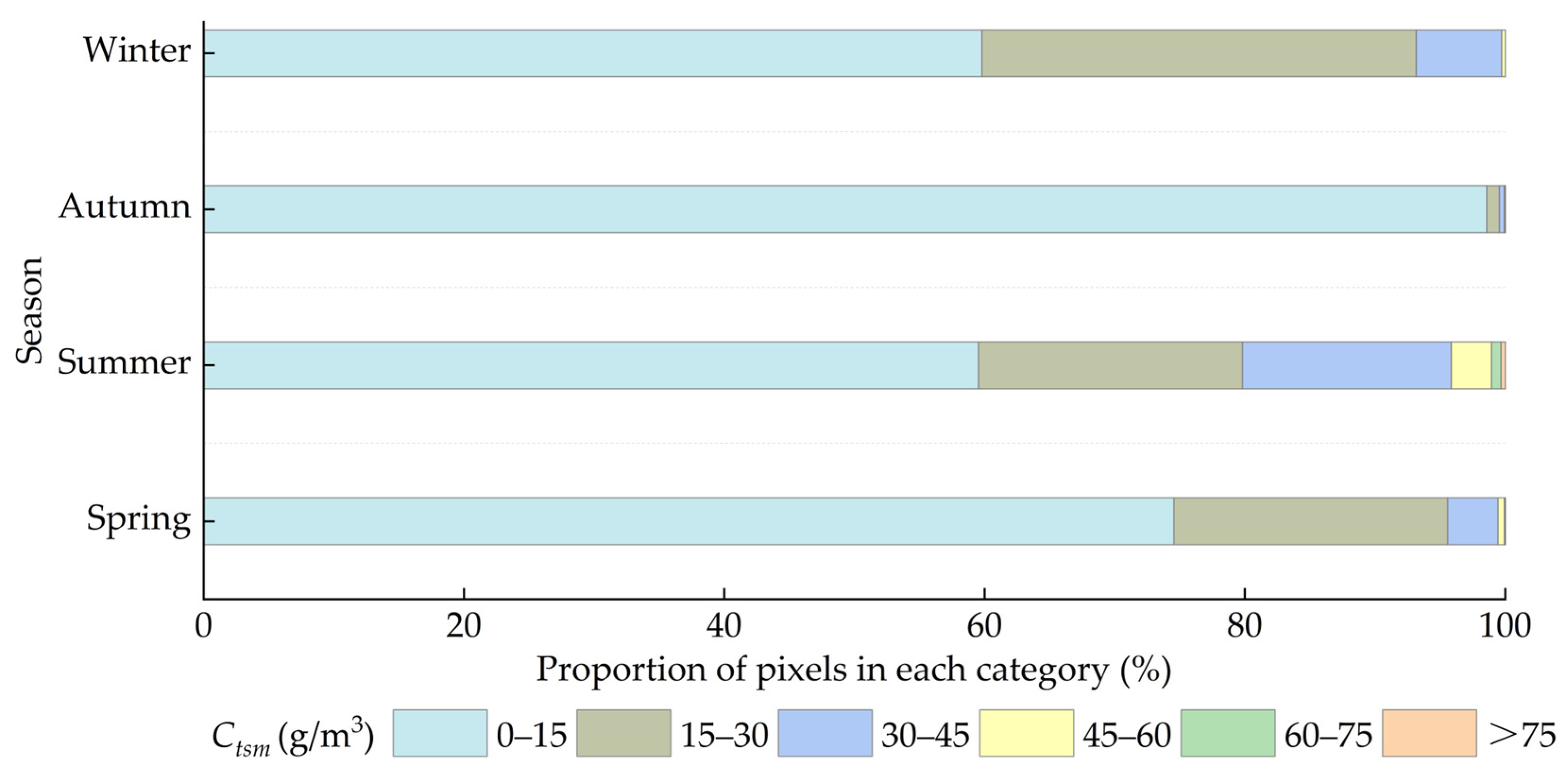
In order to analyze the temporal changes in in Lake Taihu, the inversion results of were divided into six concentration intervals, including 0–15 g/m3, 15–30 g/m3, 30–45 g/m3, 45–60 g/m3, 60–75 g/m3, and > 75 g/m3, and the proportion of image pixels of of each interval in each quarter was counted as a percentage of the overall effective image pixels. The effective pixels did not include the algal bloom pixels and the pixels covered by clouds and fog. Figure 22 shows the results of the proportion of pixels in each concentration interval in different seasons in Lake Taihu. In general, was higher in spring, summer, and winter, while it was lower in fall. Due to the small amount of available SDGSAT-1 MII images in 2022 and 2023, detailed seasonal changes will need to be determined through the long-term monitoring of data.
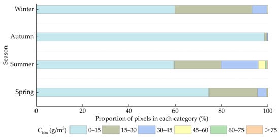
Figure 22.
Quarterly statistics of the proportion of pixels in each range of .
5. Conclusions
Considering that the composition and optical properties of inland water are affected by the concentration of different components in water, in order to overcome the interference of and in the inversion study of , this study established an iterative inversion model for estimating based on multiple linear regression based on the characteristics of SDGSAT-1 MII sensor. The Hydrolight model was used to simulate the radiative transfer process of Lake Taihu, and the influence characteristics and correlation analysis of , , and on remote sensing reflectance were carried out. On this basis, the characteristic band combinations for multiple linear regression analysis were determined. The iterative inversion model of solving is formed by combining two multivariate linear regression models. The iterative inversion model was validated using modeling data and image data, and it was compared with the iterative inversion model built with other band combinations as characteristic band combinations, as well as with other published models. Furthermore, the spatiotemporal distribution characteristics of in Lake Taihu were investigated using SDGSAT-1 MII images taken in 2022–2023. The primary conclusions of this study are as follows:
(1) The simulation of the Hydrolight model produced 54 groups of 400–800 nm simulated remote sensing reflectance of Lake Taihu, and validation revealed that the simulated spectra had a high similarity with the shape of the measured spectral curves, and the correlation between the simulated spectra and the measured spectra of each group was over 0.93, and the coefficient of determination of the two fitted together was R2 of 0.906, which provided the necessary data for the accurate inverse inversion of .
(2) Through the characterization of the influence of remote sensing reflectance and the analysis of the correlation between different bands and band combinations and the concentrations of the three components of total suspended matter, chlorophyll-a, and CDOM, the band combinations that did not correlate with and showed a significant correlation with and (r > 0.7 (p < 0.01)), and were selected as the characteristic band combinations, which provided a theoretical basis for the role of removing chlorophyll-a and CDOM in the inverse study of .
(3) The two multiple linear regression models established with and as the combination of the characteristic bands fit well, with R2 of 0.977 and 0.991, respectively; combining the relationship between the concentration of a single component and its contribution to the remote sensing reflectance, the two multiple regression models were joined to form a complete closed iterative inversion model. And applying the iterative inversion model to the modeling data and the image data, the R2 was 0.97 and 0.87, the RMSE was 4.89 g/m3 and 3.92 g/m3, and the MAPE was 11.48% and 8.13%, respectively, with strong consistency between the retrieved and the measured .
(4) Compared with the iterative inversion model based on and , the iterative inversion model based on and , the iterative inversion model based on and , and other published models, the iterative inversion model established in this paper based on and had higher accuracy and was more suitable for the SDGSAT-1 MII images of Lake Taihu, and of Lake Taihu in 2022–2023 remote sensing monitoring results showed that there were differences in the spatial distribution of , with low concentrations mainly concentrated in the center region of the lake, and lower in autumn than in the other three seasons.
Overall, the iterative inversion model developed for SDGSAT-1 MII in this study had good applicability in the Lake Taihu area. Due to the limited number of measured synchronized with the time of SDGSAT-1 satellite transit over Lake Taihu, the collection time of field sample points failed to cover four seasons, and it is a challenge to fully validate the model using multiple images. In future research, we endeavor to collect more measured synchronized with the SDGSAT-1 satellite transit time of Lake Taihu in different seasons to explore and validate the applicability of the inversion model on SDGSAT-1 satellite more comprehensively, and to provide a theoretical basis and technical support for remote sensing monitoring and improvement of the water environment in Lake Taihu and other inland water.
Author Contributions
Conceptualization, X.H. and J.L.; methodology, X.H., J.L. and Y.S. (Yuan Sun); validation, Y.S. (Yuan Sun), Y.B. and Y.S. (Yonghua Sun); formal analysis, X.H. and J.L.; resources, J.L.; writing—original draft preparation, X.H.; writing—review and editing, J.L., Y.S. (Yuan Sun), Y.B., Y.S. (Yonghua Sun) and X.C.; visualization, X.H.; supervision, J.L., X.C. and Y.Y.; funding acquisition, J.L. All authors have read and agreed to the published version of the manuscript.
Funding
This research was funded by the Civil Aerospace Technology Advance Research Project of China and the National Natural Science Foundation of China (Grant No. 41971391).
Data Availability Statement
The original contributions presented in the study are included in the article material, further inquiries can be directed to the corresponding author.
Conflicts of Interest
The authors declare no conflicts of interest.
Appendix A
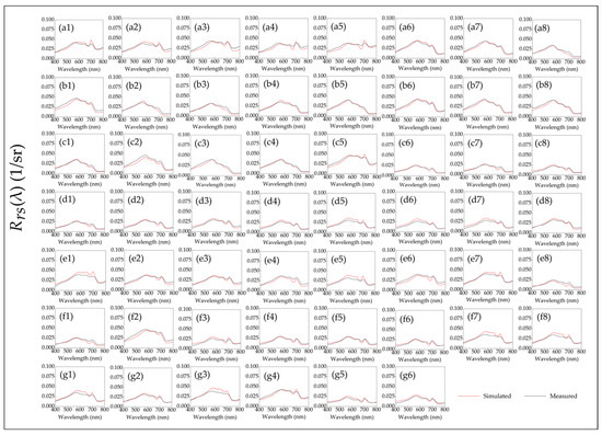
Figure A1.
Comparison between simulated and measured . (a1–a8), (b1–b8), (c1–c8), (d1–d8), (e1–e8), (f1–f8), and (g1–g6) are the comparisons of 54 groups of .
Figure A1.
Comparison between simulated and measured . (a1–a8), (b1–b8), (c1–c8), (d1–d8), (e1–e8), (f1–f8), and (g1–g6) are the comparisons of 54 groups of .
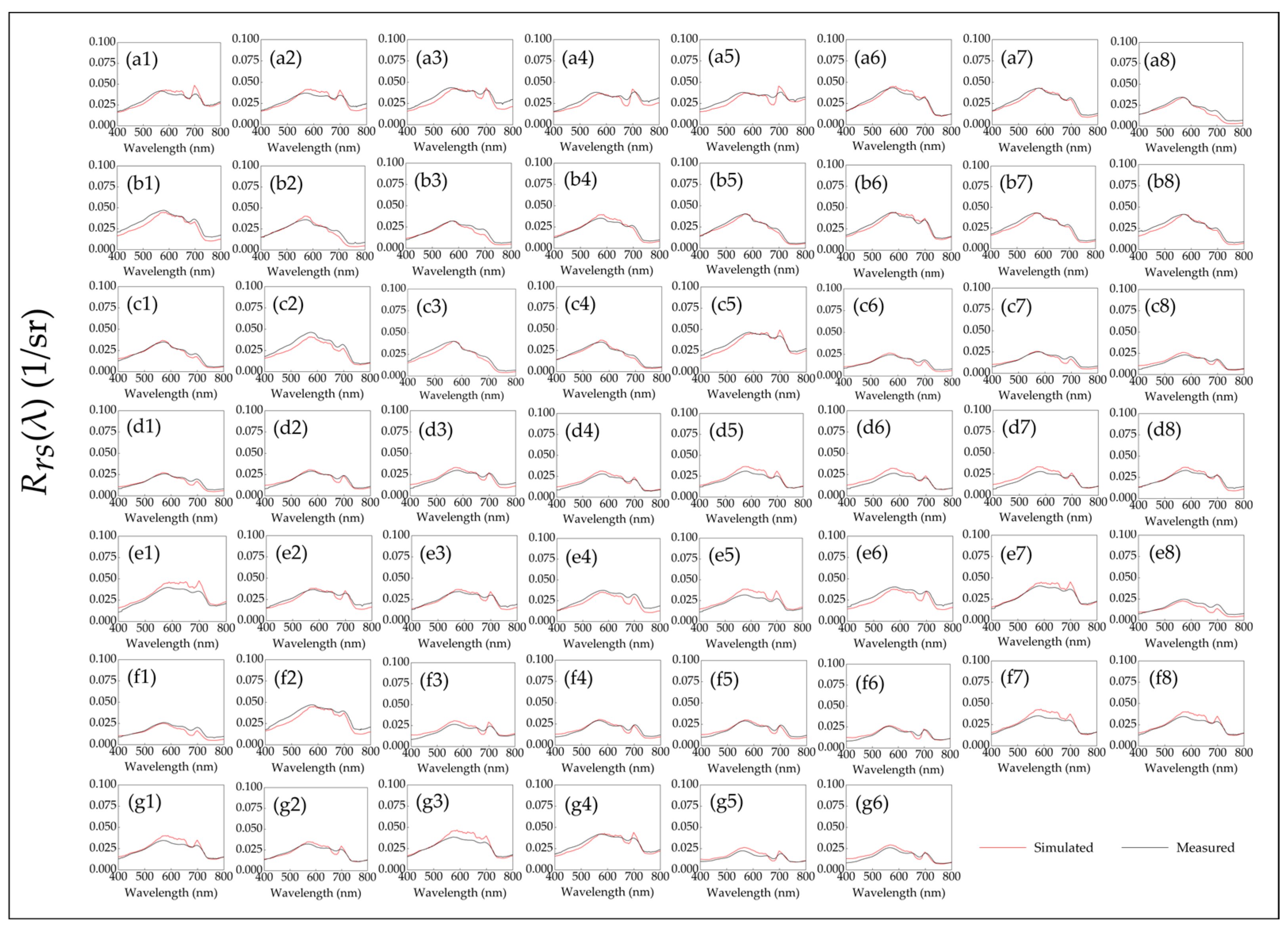

Figure A2.
Correlation analysis results: (a) correlation between and the concentrations of the three components; (b) correlation between and the concentrations of the three components; and (c) correlation between and the concentrations of the three components.
Figure A2.
Correlation analysis results: (a) correlation between and the concentrations of the three components; (b) correlation between and the concentrations of the three components; and (c) correlation between and the concentrations of the three components.
References
- Sun, M.; Zhang, L.; Yang, R.; Li, X.; Zhao, J.; Liu, Q. Water resource dynamics and protection strategies for inland lakes: A case study of Hongjiannao Lake. J. Environ. Manag. 2024, 355, 120462. [Google Scholar] [CrossRef]
- He, Y.; Lu, Z.; Wang, W.; Zhang, D.; Zhang, Y.; Qin, B.; Shi, K.; Yang, X. Water clarity mapping of global lakes using a novel hybrid deep-learning-based recurrent model with Landsat OLI images. Water Res. 2022, 215, 118241. [Google Scholar] [CrossRef] [PubMed]
- Soomets, T.; Uudeberg, K.; Jakovels, D.; Brauns, A.; Zagars, M.; Kutser, T. Validation and comparison of water quality products in baltic lakes using sentinel-2 msi and sentinel-3 OLCI data. Sensors 2020, 20, 742. [Google Scholar] [CrossRef]
- Zhai, M.; Zhou, X.; Tao, Z.; Lv, T.; Zhang, H.; Li, R.; Huang, Y. Retrieve of total suspended matter in typical lakes in China based on broad bandwidth satellite data: Random forest model with Forel-Ule Index. Front. Environ. Sci. 2023, 11, 1132346. [Google Scholar] [CrossRef]
- Li, N.; Zhang, Y.; Shi, K.; Zhang, Y.; Sun, X.; Wang, W.; Huang, X. Monitoring water transparency, total suspended matter and the beam attenuation coefficient in inland water using innovative ground-based proximal sensing technology. J. Environ. Manag. 2022, 306, 114477. [Google Scholar] [CrossRef] [PubMed]
- Tian, L.; Wai, O.W.; Chen, X.; Li, W.; Li, J.; Li, W.; Zhang, H. Retrieval of total suspended matter concentration from Gaofen-1 Wide Field Imager (WFI) multispectral imagery with the assistance of Terra MODIS in turbid water–case in Deep Bay. Int. J. Remote Sens. 2016, 37, 3400–3413. [Google Scholar] [CrossRef]
- Xiong, Y.; Ran, Y.; Zhao, S.; Zhao, H.; Tian, Q. Remotely assessing and monitoring coastal and inland water quality in China: Progress, challenges and outlook. Crit. Rev. Environ. Sci. Technol. 2020, 50, 1266–1302. [Google Scholar] [CrossRef]
- Ge, K.; Liu, J.; Wang, F.; Chen, B.; Hu, Y. A Cloud Detection Method Based on Spectral and Gradient Features for SDGSAT-1 Multispectral Images. Remote Sens. 2022, 15, 24. [Google Scholar] [CrossRef]
- Shen, M.; Luo, J.; Cao, Z.; Xue, K.; Qi, T.; Ma, J.; Liu, D.; Song, K.; Feng, L.; Duan, H. Random forest: An optimal chlorophyll-a algorithm for optically complex inland water suffering atmospheric correction uncertainties. J. Hydrol. 2022, 615, 128685. [Google Scholar] [CrossRef]
- Silveira Kupssinskü, L.; Thomassim Guimarães, T.; Menezes de Souza, E.; Zanotta, D.C.; Roberto Veronez, M.; Gonzaga, L., Jr.; Mauad, F.F. A method for chlorophyll-a and suspended solids prediction through remote sensing and machine learning. Sensors 2020, 20, 2125. [Google Scholar] [CrossRef]
- Liu, J.; Liu, J.; He, X.; Pan, D.; Bai, Y.; Zhu, F.; Chen, T.; Wang, Y. Diurnal dynamics and seasonal variations of total suspended particulate matter in highly turbid hangzhou bay waters based on the geostationary ocean color imager. IEEE J. Sel. Top. Appl. Earth Observ. Remote Sens. 2018, 11, 2170–2180. [Google Scholar] [CrossRef]
- Wen, Z.; Wang, Q.; Liu, G.; Jacinthe, P.-A.; Wang, X.; Lyu, L.; Tao, H.; Ma, Y.; Duan, H.; Shang, Y. Remote sensing of total suspended matter concentration in lakes across China using Landsat images and Google Earth Engine. ISPRS-J. Photogramm. Remote Sens. 2022, 187, 61–78. [Google Scholar] [CrossRef]
- Tang, Y.; Pan, Y.; Zhang, L.; Yi, H.; Gu, Y.; Sun, W. Efficient Monitoring of Total Suspended Matter in Urban Water Based on UAV Multi-spectral Images. Water Resour. Manag. 2023, 37, 2143–2160. [Google Scholar] [CrossRef]
- Wang, C.; Wang, D.; Yang, J.; Fu, S.; Li, D. Suspended Sediment within Estuaries and along Coasts: A Review of Spatial and Temporal Variations based on Remote Sensing. J. Coast. Res. 2020, 36, 1323–1331. [Google Scholar] [CrossRef]
- Xu, J.; Zhang, B.; Song, K.; Wang, Z.; Duan, H.; Chen, M.; Yang, F.; Li, F. Bio-Optical model of total suspended matter based on reflectance in the near infrared wave band for Case-II waters. Spectrosc. Spectr. Anal. 2008, 28, 2273–2277. [Google Scholar]
- Werdell, P.J.; McKinna, L.I.; Boss, E.; Ackleson, S.G.; Craig, S.E.; Gregg, W.W.; Lee, Z.; Maritorena, S.; Roesler, C.S.; Rousseaux, C.S. An overview of approaches and challenges for retrieving marine inherent optical properties from ocean color remote sensing. Prog. Oceanogr. 2018, 160, 186–212. [Google Scholar] [CrossRef]
- Chen, S.; Han, L.; Chen, X.; Li, D.; Sun, L.; Li, Y. Estimating wide range Total Suspended Solids concentrations from MODIS 250-m imageries: An improved method. ISPRS-J. Photogramm. Remote Sens. 2015, 99, 58–69. [Google Scholar] [CrossRef]
- Hou, X.; Feng, L.; Duan, H.; Chen, X.; Sun, D.; Shi, K. Fifteen-year monitoring of the turbidity dynamics in large lakes and reservoirs in the middle and lower basin of the Yangtze River, China. Remote Sens. Environ. 2017, 190, 107–121. [Google Scholar] [CrossRef]
- Li, W.; Yang, Q.; Ma, Y.; Yang, Y.; Song, K.; Zhang, J.; Wen, Z.; Liu, G. Remote Sensing Estimation of Long-Term Total Suspended Matter Concentration from Landsat across Lake Qinghai. Water 2022, 14, 2498. [Google Scholar] [CrossRef]
- Wang, C.; Chen, S.; Li, D.; Wang, D.; Liu, W.; Yang, J. A Landsat-based model for retrieving total suspended solids concentration of estuaries and coasts in China. Geosci. Model Dev. 2017, 10, 4347–4365. [Google Scholar] [CrossRef]
- Adhikari, A.; Menon, H.B. A Bio-optical Numerical Approach for Remote Retrieval of Total Suspended Matter from Turbid Waters. J. Indian Soc. Remote Sens. 2022, 50, 1773–1786. [Google Scholar] [CrossRef]
- Pahlevan, N.; Sarkar, S.; Franz, B.; Balasubramanian, S.V.; He, J. Sentinel-2 MultiSpectral Instrument (MSI) data processing for aquatic science applications: Demonstrations and validations. Remote Sens. Environ. 2017, 201, 47–56. [Google Scholar] [CrossRef]
- Jiang, D.; Matsushita, B.; Pahlevan, N.; Gurlin, D.; Lehmann, M.K.; Fichot, C.G.; Schalles, J.; Loisel, H.; Binding, C.; Zhang, Y. Remotely estimating total suspended solids concentration in clear to extremely turbid waters using a novel semi-analytical method. Remote Sens. Environ. 2021, 258, 112386. [Google Scholar] [CrossRef]
- Liu, Z.; Chen, J.; Cui, T.; Tang, J.; Wang, L. A combined semi-analytical algorithm for retrieving total suspended sediment concentration from multiple missions: A case study of the China Eastern Coastal Zone. Int. J. Remote Sens. 2021, 42, 8004–8033. [Google Scholar] [CrossRef]
- Kang, L.; Zhu, G.; Zhu, M.; Xu, H.; Zou, W.; Xiao, M.; Zhang, Y.; Qin, B. Bloom-induced internal release controlling phosphorus dynamics in large shallow eutrophic Lake Taihu, China. Environ. Res. 2023, 231, 116251. [Google Scholar] [CrossRef] [PubMed]
- Yang, W.; Matsushita, B.; Chen, J.; Fukushima, T. A relaxed matrix inversion method for retrieving water constituent concentrations in case II waters: The case of Lake Kasumigaura, Japan. IEEE Trans. Geosci. Remote Sens. 2011, 49, 3381–3392. [Google Scholar] [CrossRef]
- Liu, C.-C.; Miller, R.L. Spectrum matching method for estimating the chlorophyll-a concentration, CDOM ratio, and backscatter fraction from remote sensing of ocean color. Can. J. Remote Sens. 2008, 34, 343–355. [Google Scholar] [CrossRef]
- Zhang, Y.; Ma, R.; Duan, H.; Loiselle, S.; Xu, J. A spectral decomposition algorithm for estimating chlorophyll-a concentrations in Lake Taihu, China. Remote Sens. 2014, 6, 5090–5106. [Google Scholar] [CrossRef]
- Qin, B.; Deng, J.; Shi, K.; Wang, J.; Brookes, J.; Zhou, J.; Zhang, Y.; Zhu, G.; Paerl, H.W.; Wu, L. Extreme climate anomalies enhancing cyanobacterial blooms in eutrophic Lake Taihu, China. Water Resour. Res. 2021, 57, e2020WR029371. [Google Scholar] [CrossRef]
- Ma, R.; Duan, H.; Liu, Q.; Loiselle, S.A. Approximate bottom contribution to remote sensing reflectance in Taihu Lake, China. J. Gt. Lakes Res. 2011, 37, 18–25. [Google Scholar] [CrossRef]
- Clementson, L.A.; Parslow, J.S.; Turnbull, A.R.; McKenzie, D.C.; Rathbone, C.E. Optical properties of waters in the Australasian sector of the Southern Ocean. J. Geophys. Res. Oceans 2001, 106, 31611–31625. [Google Scholar] [CrossRef]
- Stramska, M.; Stramski, D.; Mitchell, B.G.; Mobley, C.D. Estimation of the absorption and backscattering coefficients from inߚwater radiometric measurements. Limnol. Oceanogr. 2000, 45, 628–641. [Google Scholar] [CrossRef]
- Kim, J.; Jang, W.; Kim, J.H.; Lee, J.; Cho, K.H.; Lee, Y.-G.; Chon, K.; Park, S.; Pyo, J.; Park, Y. Application of airborne hyperspectral imagery to retrieve spatiotemporal CDOM distribution using machine learning in a reservoir. Int. J. Appl. Earth Obs. Geoinf. 2022, 114, 103053. [Google Scholar] [CrossRef]
- Zhang, F.; Li, J.; Wang, C.; Wang, S.; Wang, Z.; Zhang, B. Multitype inland water atmospheric correction and water quality estimation based on HY-1C CZI images. Natl. Remote Sens. Bull. 2023, 27, 79–91. [Google Scholar] [CrossRef]
- Tang, J.-W.; Tian, G.-L.; Wang, X.-Y.; Wang, X.-M.; Song, Q.-J. The methods of water spectra measurement and analysis I: Above-Water method. J. Remote Sens. 2021, 1, 37–44. [Google Scholar]
- Pancorbo, J.; Lamb, B.T.; Quemada, M.; Hively, W.D.; Gonzalez-Fernandez, I.; Molina, I. Sentinel-2 and WorldView-3 atmospheric correction and signal normalization based on ground-truth spectroradiometric measurements. ISPRS-J. Photogramm. Remote Sens. 2021, 173, 166–180. [Google Scholar] [CrossRef]
- Wang, R.; Shen, Q.; Peng, H.; Yao, Y.; Li, J.; Wang, M.; Shi, J.; Xu, W. Study on the applicability of multi-source high-resolution satellite images for monitoring black and odorous water body. Natl. Remote Sens. Bull. 2022, 26, 179–192. [Google Scholar] [CrossRef]
- Zhao, Z.; Yang, J.; Wang, M.; Chen, J.; Sun, C.; Song, N.; Wang, J.; Feng, S. The PCA-NDWI Urban Water Extraction Model Based on Hyperspectral Remote Sensing. Water 2024, 16, 963. [Google Scholar] [CrossRef]
- Werdell, P.J.; Franz, B.A.; Bailey, S.W.; Feldman, G.C.; Boss, E.; Brando, V.E.; Dowell, M.; Hirata, T.; Lavender, S.J.; Lee, Z. Generalized ocean color inversion model for retrieving marine inherent optical properties. Appl. Optics. 2013, 52, 2019–2037. [Google Scholar] [CrossRef]
- Pope, R.M.; Fry, E.S. Absorption spectrum (380–700 nm) of pure water. II. Integrating cavity measurements. Appl. Opt. 1997, 36, 8710–8723. [Google Scholar] [CrossRef]
- Mohd-Shazali, S.M.; Madihah, J.-S.; Ali, N.; Cheng-Ann, C.; Brewin, R.J.; Idris, M.S.; Noir, P.P. Dynamics of absorption properties of CDOM and its composition in Likas estuary, North Borneo, Malaysia. Oceanologia 2022, 64, 583–594. [Google Scholar] [CrossRef]
- Smith, R.C.; Baker, K.S. Optical properties of the clearest natural waters (200–800 nm). Appl. Opt. 1981, 20, 177–184. [Google Scholar] [CrossRef] [PubMed]
- Li, Y.; Wang, Q.; Huang, J.; Lyu, H.; Wei, Y. Optical Characteristics and Remote Sensing of Water Color in Lake Taihu; Science Press: Beijing, China, 2010; pp. 129–137. [Google Scholar]
- Miller, J.D.; Thode, A.E. Quantifying burn severity in a heterogeneous landscape with a relative version of the delta Normalized Burn Ratio (dNBR). Remote Sens. Environ. 2007, 109, 66–80. [Google Scholar] [CrossRef]
- Su, H.; Lu, X.; Chen, Z.; Zhang, H.; Lu, W.; Wu, W. Estimating coastal chlorophyll-a concentration from time-series OLCI data based on machine learning. Remote Sens. 2021, 13, 576. [Google Scholar] [CrossRef]
- Wang, J.-H.; Li, C.; Xu, Y.-P.; Li, S.-Y.; Du, J.-S.; Han, Y.-P.; Hu, H.-Y. Identifying major contributors to algal blooms in Lake Dianchi by analyzing river-lake water quality correlations in the watershed. J. Clean. Prod. 2021, 315, 128144. [Google Scholar] [CrossRef]
- Shi, K.; Zhang, Y.; Zhu, G.; Liu, X.; Zhou, Y.; Xu, H.; Qin, B.; Liu, G.; Li, Y. Long-term remote monitoring of total suspended matter concentration in Lake Taihu using 250 m MODIS-Aqua data. Remote Sens. 2015, 164, 43–56. [Google Scholar]
- Li, J.; Chen, X.; Tian, L.; Huang, J.; Feng, L. Improved capabilities of the Chinese high-resolution remote sensing satellite GF-1 for monitoring suspended particulate matter (SPM) in inland waters: Radiometric and spatial considerations. ISPRS-J. Photogramm. Remote Sens. 2015, 106, 145–156. [Google Scholar] [CrossRef]

Disclaimer/Publisher’s Note: The statements, opinions and data contained in all publications are solely those of the individual author(s) and contributor(s) and not of MDPI and/or the editor(s). MDPI and/or the editor(s) disclaim responsibility for any injury to people or property resulting from any ideas, methods, instructions or products referred to in the content. |
© 2024 by the authors. Licensee MDPI, Basel, Switzerland. This article is an open access article distributed under the terms and conditions of the Creative Commons Attribution (CC BY) license (https://creativecommons.org/licenses/by/4.0/).