Abstract
With the wide application of UAVs in modern intelligent warfare as well as in civil fields, the demand for C-UAS technology is increasingly urgent. Traditional detection methods have many limitations in dealing with “low, slow, and small” targets. This paper presents a pure laser automatic tracking system based on Geiger-mode avalanche photodiode (Gm-APD). Combining the target motion state prediction of the Kalman filter and the adaptive target tracking of Camshift, a Cam–Kalm algorithm is proposed to achieve high-precision and stable tracking of moving targets. The proposed system also introduces two-dimensional Gaussian fitting and edge detection algorithms to automatically determine the target’s center position and the tracking rectangular box, thereby improving the automation of target tracking. Experimental results show that the system designed in this paper can effectively track UAVs in a 70 m laboratory environment and a 3.07 km to 3.32 km long-distance scene while achieving low center positioning error and MSE. This technology provides a new solution for real-time tracking and ranging of long-distance UAVs, shows the potential of pure laser approaches in long-distancelow, slow, and small target tracking, and provides essential technical support for C-UAS technology.
1. Introduction
Uncrewed Aerial Vehicles (UAVs), as a representative type of low, slow and small target, have the advantages of good concealment, anti-jamming solid ability, low requirements for landing environment, and low cost. They are gradually being put into operational use and have become essential to intelligence, early warning, and reconnaissance equipment in various countries [1,2]. At the same time, with the rapid expansion of the civilian UAV market, related security risks have become increasingly apparent, posing a severe threat to civil aviation traffic, social security, and personal privacy [3,4]. In January 2015, a DJI Elf UAV crashed into the White House in the United States [5,6]. Since then, the phenomenon of “black flying” and “indiscriminate flying” of UAVs has been repeatedly banned. In May 2017, Kunming Kunming Changshui International Airport, China was disturbed by drones, resulting in the forced landing of 35 flights and the closure of the airport runway for 45 min [7]. In August 2018, Venezuelan President Maduro was attacked by a drone during a televised speech, further causing social panic [6,8,9].
Therefore, developing early warning and defense technology for UAVs has become an urgent problem for all countries [10,11]. At present, detection methods for low-altitude UAVs include radar early warning, passive imaging detection, acoustic array detection, and other technologies, among which are the following [6,12,13]:
- Radar early warning technology:
- (1)
- American Echo Shield 4D radar combines Ku-band BSA beamforming and dynamic waveform synthesis 6 [14]. It offers wireless positioning service at 15.7–16.6 GHz and wireless navigation function at 15.4–15.7 GHz, with a tracking accuracy of 0.5° and an effective detection distance of 3 km.
- (2)
- HARRIER DSR UAV surveillance radar developed by DeTecT Company of the United States adopts a solid-state Doppler detection radar system, which is used for small RCS targets in complex clutter environments. The detection range of UAVs flying without RF and GPS programs is 3.2 km [15].
- (3)
- Hof Institute of High-Frequency Physics and Radar Technology in Flawn, Germany has proposed Scanning Surveillance Radar System (SSRS) technology [16]. The FMCW radar sensor is scanned mechanically, with a scanning frequency of 8 Hz and a bandwidth of 1 GHz. The maximum range resolution is 15 cm, and the maximum detection range is 153.6 m.
- Passive optical imaging technology [17]:
- (1)
- Poland Advanced Protection System Company has designed the SKYctrl anti-UAV system, which includes an ultra-precision FIELDctrl 3D MIMO radar, PTZ day/night camera, WiFi sensor, and acoustic array. The detecting target’s minimum height is 1 m.
- (2)
- France’s France–Germany Institute in Saint Louis has adopted two optical sensing channels, while a passive color camera provides the image of the target area with a field of view of 4° × 3° and can detect a DJI UAV from 100 m to 200 m.
- (3)
- The National Defense Development Agency of Korea has proposed a UAV tracking method using KCF and adaptive thresholding. The system includes a visual camera, pan/tilt, image processing system, pan/tilt control computer, driving system, and a liquid crystal display that can detect the UAV with a target size of about 30 × 30 cm, flying speed of about 10 m/s, and distance of 1.5 km.
- (4)
- DMA’s low-altitude early warning and tracking photoelectric system developed by China Hepu Company integrates a high-definition visible-light camera and an infrared imaging sensor. The system can detect micro-UAVs within 2 km, and the tracking angular velocity can reach 200°.
- Acoustic detection technology:
- (1)
- Dedrone Company of Germany has developed Drone Tracker, a UAV detection system that uses distributed acoustic and optical sensors to comprehensively detect UAVs. It can detect illegally invading UAVs 50–80 m in advance [18].
- (2)
- Holy Cross University of Technology in Poland studied the acoustic signal of a rotary-wing UAV; using an Olympus LS-11 digital recorder, the acoustic signal was recorded at a 44 kHz sampling rate and 16-bit signal resolution, and was obtained at a distance as far as 200 m.
However, the concealment and flexibility of low, slow, and small UAVs mean that existing detection technologies face many challenges [19,20]:
- The targets are small and difficult to detect: The reflection cross-section of UAV radar is actively tiny, making it difficult for traditional radar to capture effectively.
- Complex background interference: Interference is greatly influenced by ground clutter, which increases the difficulty of detection.
- Low noise and low infrared radiation: The sound wave and infrared characteristics generated by UAVs are weak, making them difficult to detect via sound wave or infrared detection.
- Significant environmental impact: Weather conditions such as smog and rainy days affect the performance of traditional optical and acoustic detection.
Compared with the above technologies, single-photon LiDAR has a number of apparent advantages. By actively emitting narrow beam laser for detection, clutter interference is effectively reduced; in addition, it can respond to a single echo photon and still capture a weak echo signal in complex environments, which is especially suitable for long-distance detection of small and low-reflection targets. Such LiDARs have strong ability to resist weather interference, are able to work all day in day and night and during light fog. Their nanoscale time resolution can locate the target in real-time and high-precision three-dimensional space. The high-precision and high-sensitivity technology of single-photon LiDAR breaks through the limitations of traditional technology in terms of detection range, resolution, and anti-interference capability, helping to make up for the shortcomings of traditional detection technologies [21,22,23].
In recent years, with the continuous development of high-frequency lasers [23], time-dependent single-photon counting (TCSPC) technology [24,25], and semiconductor photodetectors [26,27,28,29,30], the performance of Gm-APD single-photon LiDARs based on area array detection has been significantly improved. Compared with LiDARs based on Lm-APD, PMT, Si-PMT, or SP-SPD [31,32], Gm-APD detectors have a higher degree of avalanche ionization and an enormous pixel array. Their application has been studied in the field of multi-concentration and long-distance fast three-dimensional or biological imaging [33,34,35,36,37,38,39,40]. However, the existing research on UAV early warning detection still needs to be improved, and further exploration is needed. In 2021, Ding Yuanxue of the Harbin Institute of Technology, along with others, proposed an improved YOLOv3 network detection method based on the Gm-APD LiDAR [41]. Although real-time detection was realized within a 238 m range, the tracking problem of UAVs still needs to be solved.
This paper proposes a method for detecting and tracking UAVs based on area-array Gm-APD LiDAR [42]. Automatic target extraction is realized by improving the two-dimensional Gaussian model [43], while automatic tracking is realized by combining Kalman filtering [44] and the Camshift tracking algorithm [45] into a new Cam–Kalm algorithm.
The research ob moving object tracking focuses on machine vision, for which both Camshift and particle filter algorithms are widely studied and used [46,47]. The particle filter algorithm has good ability to track targets; however, its complexity greatly influences real-time performance [48]. Compared with the particle filter algorithm, the Camshift algorithm based on color features is more straightforward and can achieve a better tracking effect [49]. Target tracking algorithms in machine vision rely on the initial appearance model (color, shape, texture, etc.) for subsequent tracking. In a complex environment, factors such as background noise, illumination changes, occlusion, and more tend to increase the similarity between the tracked object and the background, increasing the risk of false and missed detection. Therefore, it is necessary to accurately calibrate the initial target through manual intervention in order to ensure that the algorithm can accurately lock the target from the beginning and reduce errors in subsequent tracking.
Compared with the characteristics of machine vision imaging, the echo signal of a single-photon LiDAR shows a noticeable intensity gradient difference between the target and background, and shows a point spread distribution. In addition, single-photon LiDARs are insensitive to environmental illumination and other factors, and can automatically identify the target position and track it through physical quantities such as signal strength, time delay, and echo characteristics. Based on these characteristics, this paper improves the two-dimensional Gaussian model for target detection and extraction and combines the active sensing characteristics of single-photon LiDAR to achieve higher detection accuracy and environmental robustness, allowing for automatic tracking without human intervention [50,51]. Then, the proposed algorithm fusing Kalman filtering and Camshift is designed to increase the ability to predict the speed and acceleration of the target, further improving tracking accuracy and real-time performance [52,53,54]. The performance of the Cam–Kalm algorithm and traditional tracking algorithms is evaluated through a close-range experiment in the range of 70 m to 100 m. Finally, dynamic tracking of UAVs in the range of 3077.8 m to 3320.3 m is realized.
The structure of this paper is as follows: the first section introduces the research background, the second describes the area-array Gm-APD LiDAR imaging system, the third describes the designed automatic tracking algorithm, and the fourth analyzes the tracking results. Finally, the conclusions and future research prospects are summarized.
2. System Design
2.1. Design of Gm-APD LiDAR System
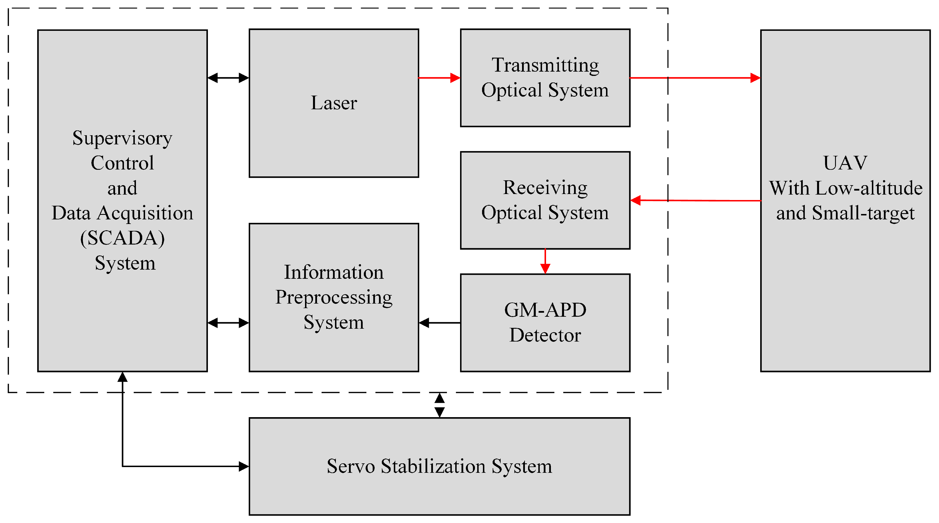
Figure 1 shows the design of the LiDAR imaging system based on the area-array Gm-APD. The system consists of five subsystems: the transmitting laser system, receiving laser system, Gm-APD detector, data acquisition and processing system based on FPGA, and servo system. The output wavelength of the laser is 1064 nm, the output power is dynamically adjustable between 0 and 30 W, and the repetition frequency is 20 kHz. The pixel number of the Gm-APD detector is 64 × 64. The power consumption of the single-photon LiDAR is less than 30 W. After being integrated into the servo turntable, the overall power consumption is less than 80 W. The servo system is equipped with a LiDAR imaging system to realize dynamic tracking. The data acquisition and processing system is responsible for the control of laser equipment, communication with the upper computer, and sending control instructions for the two-dimensional servo turntable.
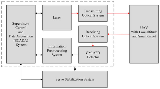
Figure 1.
Principle block diagram of Gm-APD LiDAR system.
2.2. Detection Process of Gm-APD LiDAR Imaging System
- (1)
- Laser emission: The high-power and narrow-pulse laser is pointed to the UAV target after optical shaping.
- (2)
- Laser echo reception: Echo photons reflected by the target are converged on the Gm-APD detector through the receiving optical system, triggering the avalanche effect.
- (3)
- Signal recording: The Gm-APD detector records the echo signal and transmits it to the FPGA data acquisition and processing system.
- (4)
- Signal processing: The acquisition system processes the signal and reconstructs the intensity image and range image of the UAV target.
- (5)
- Target fitting and tracking: Threshold filtering, Gaussian fitting, and canny edge detection methods are adopted, and the combined Cam–Kalm algorithm is utilized to realize real-time automatic target tracking.
- (6)
- Dynamic adjustment: The FPGA system calculates the angle according to the miss distance, adjusts the pitch or azimuth of the servo platform, and dynamically tracks the target.
3. Description of Tracking Algorithm
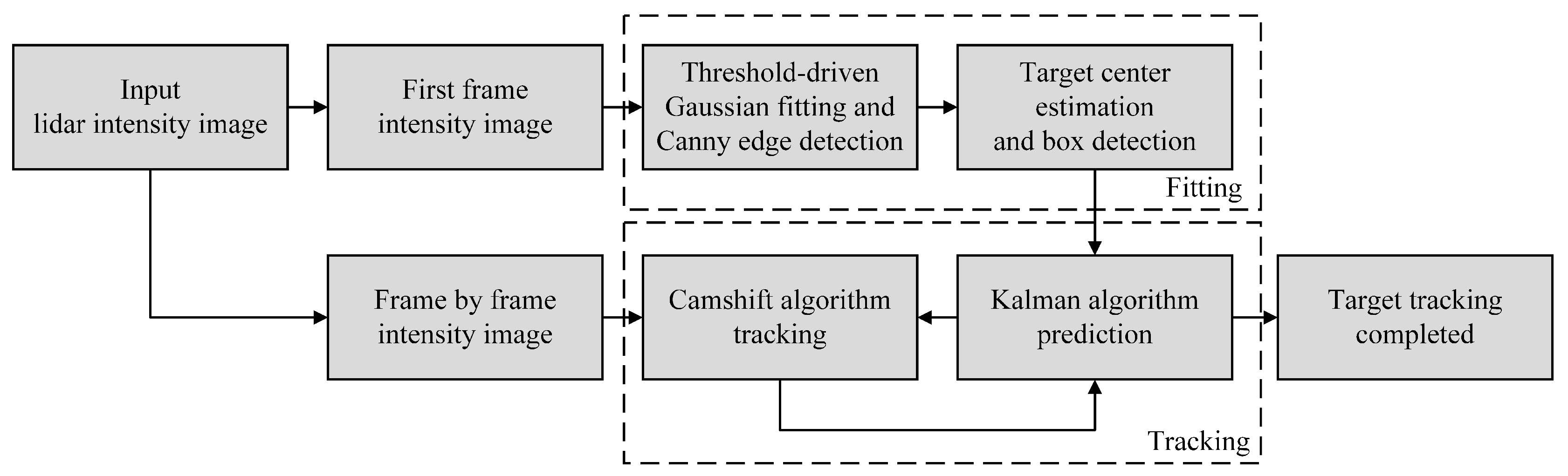
This section proposes the Cam–Kalm automatic target tracking algorithm based on the Gm-APD LiDAR imaging system, as shown in Figure 2. The algorithm mainly includes two essential parts, namely, target fitting and tracking. Below, these two parts are introduced in detail.

Figure 2.
Schematic diagram of automatic tracking algorithm.
3.1. Target Extraction
Compared with the false “noise targets” in the natural environment, the geometry of the UAV target is more regular. Using this feature effectively is the key to fitting and detection of the tracking target centers. In gray morphological analysis [55] of LiDAR intensity images, UAV targets usually appear convex in pixel values compared with the background, showing noticeable gray differences, that is, the UAV target has an additive relationship with the background information in the LiDAR intensity sequence, which can be expressed as follows:
where is the intensity value of the LiDAR, is the intensity value of the target, is the intensity value of the background, is the intensity value of noise, is the pixel coordinate in the intensity image, and t is the frame sequence number corresponding to the intensity image.
In the literature [56], the optical diffusion function is taken as the core. This function describes the expression of the ideal gray distribution of UAV targets in airspace:
where is the pixel intensity of the target at a specific time and position, (,) is the centroid of the target, is the center intensity of the target at this moment, which is generally stable between adjacent frames, and and represent the standard deviation of the target in the X and Y directions of the two-dimensional space, respectively.
According to Equation (2), the standard target Gaussian shape is established as shown in Figure 3a, where the core strength is 80 and the center position is located at . Figure 3b shows the spatial intensity distribution of real UAV targets detected by the Gm-APD LiDAR.
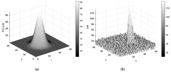
Figure 3.
Comparison of intensity distribution between standard Gaussian model and real target. (a) Based on the standard target, the Gaussian shape scale is 64 × 64 neighborhood space shape. (b) Intensity distribution of real UAV target based on Gm-APD LiDAR.
When comparing the spatial distribution scale of the set target with the imaging results of the Gm-APD LiDAR:
- (1)
- There is little difference between the spatial distribution of the target intensity image and the geometric ideal shape.
- (2)
- The actual detected target presents an irregular convex pattern relative to the background, consistent with the smooth central convex feature of the standard model.
Based on this, we use a two-dimensional Gaussian model to fit the gray morphology of the target; the algorithm flow is shown in Figure 4. The target intensity in the intensity image of the LiDAR is higher than the background noise. We use the percentage threshold filtering method to remove the low-intensity background and keep the high-intensity signal. Using two-dimensional Gaussian fitting to obtain the target centroid as the tracking center, canny edge detection [57] is used to detect the region of intensity image, then the connected region attribute is extracted using the Regionprops function [58] to determine the region of interest (ROI) of the target, that is, the bounding box of the tracking target.
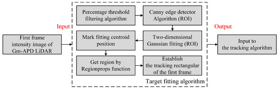
Figure 4.
Algorithm flow of target center fitting.
The LiDAR intensity image and the filtering result are shown in Figure 5. The filtered result is fitted; the fitting result is shown in Figure 6. The red circle in Figure 6a is the fitted target center position, and the red dotted line in Figure 6b is the detected tracking frame.
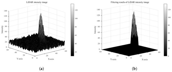
Figure 5.
LiDAR intensity image and threshold filtering results. (a) Intensity image of LiDAR. (b) Algorithm filtering result.
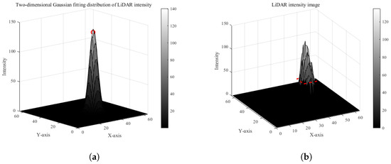
Figure 6.
Target center estimation and tracking frame detection results: (a) detection results of target tracking center and (b) detection results of tracking rectangle.
Through the above fitting algorithm, we can accurately mark the center position of the target in the intensity image of the LiDAR and complete the extraction of the ROI region through the canny edge detection algorithm, which provides the target center position and tracking rectangular box of the first frame for the follow-up tracking algorithm.
3.2. Target Tracking and State Prediction
Recognizing the particularity of UAV tracking in airspace, a Kalman filtering algorithm is introduced for the following three purposes [53]:
- (1)
- Increase forecasting ability: Based on the target position prediction, velocity and acceleration variables are introduced to improve the adaptability to the rapid change of UAV position; this not only improves the system’s robustness but also reduces the iterative calculation of the Camshift algorithm and accelerates the coordination with the two-dimensional tracking platform.
- (2)
- Reduce the false alarm rate: By predicting the speed and acceleration of the target, the moving trend of the target can be judged and the influence of ghosts in LiDAR imaging can be reduced, thereby reducing the false alarm rate.
- (3)
- Adaptive adjustment of search window: Adaptive adjustment of the search window can be realized to effectively solve the problem of loss of the tracking target caused by the Camshift algorithm’s expansion of the tracking window.
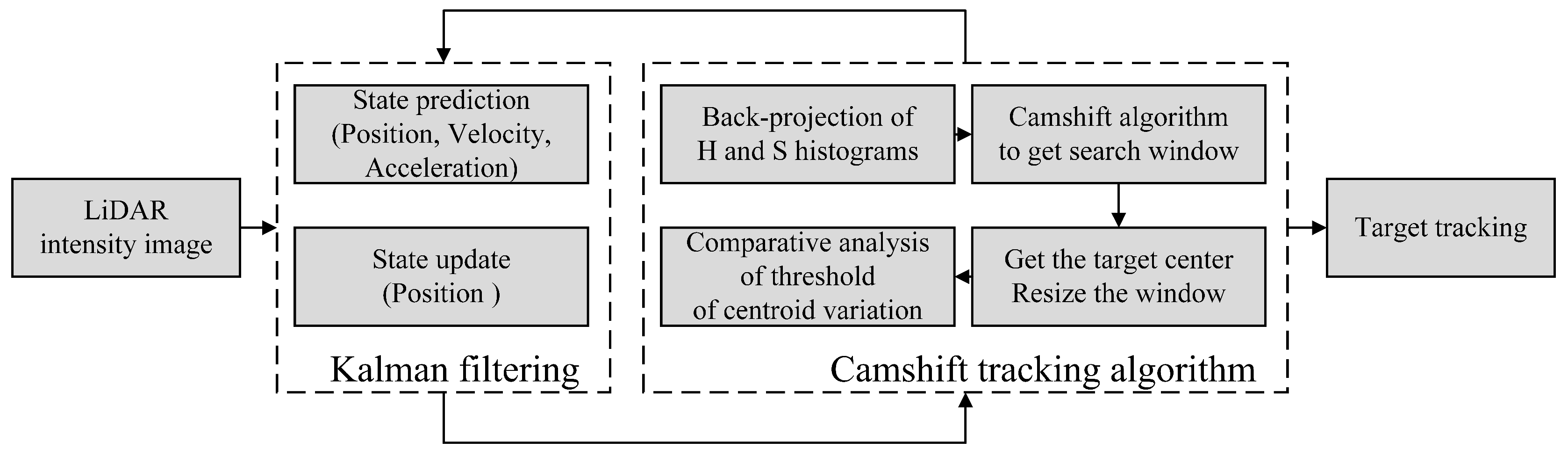
The tracking algorithm flow is shown in Figure 7.
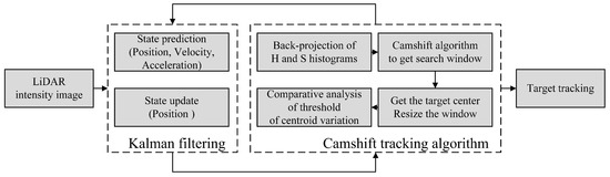
Figure 7.
Principle block diagram of Cam–Kalm tracking algorithm.
- Step 1
- Initialization.
- (1)
- Automatic extraction of the first frame target. We use the fitting method in Section 3.1 to obtain the ROI of the target point and synchronously initialize the center position and size of the search window.
- (2)
- Initialize the Kalman filter. The state prediction equation and the observation equation of the tracking system is as follows:where and represent the motion state vectors of and , respectively, is the system state observation vector at the moment, A is the state transition matrix, containing the dynamic model of target position, velocity, and acceleration, H is the observation matrix indicating the position of direct observation, and and respectively represent the system state noise and the observed Gaussian distribution noise matrix [59]:where is the time interval between two adjacent frames. Accordingly, the covariance matrix of and corresponds to Q and R, representing the uncertainty in the modeling process and the observed noise respectively, for which the formula is updated to:
- Step 2
- Backproject the histogram of the LiDAR intensity image.
- (1)
- Target area calculation. The intensity image of the first frame of the Gm-APD LiDAR is read and the pixel intensity distribution of the automatically detected target area is calculated.
- (2)
- Backprojecting the histogram of the search area. Each pixel value is mapped to the corresponding probability value in the target histogram to generate a backprojection.
- Step 3
- Calculate the search window.The centroid of the range profile search window of the LiDAR is calculated using its zero-order moment and first-order moment; represents the pixel values at in the back projection image, where x and y change within the search window . The calculation steps are as follows:
- (1)
- Calculate the zero-order moment at the initial moment:
- (2)
- Calculate the first moment in the x and y directions::
- (3)
- Calculate the centroid coordinates of the tracking window:
- (4)
- Move the center of the search window to the center-of-mass position .
- Step 4
- Calculate the trace window.The Camshift algorithm obtains the directional target area through the second-order matrix:
- (1)
- Calculate the second moment in the x and y directions:
- (2)
- Calculate the new tracking window size () as follows:among which:
- (3)
- Iterate continuously until the centroid position converges. The centroid of the target point is the iterative result , which is used to update and predict the Kalman filtering time .
- Step 5
- Kalman filter prediction.At moment , the state vector of UAV target motion iswhere and represent the speed of the target in the X and Y axis directions within the field of view and and represent the target’s acceleration. According to Equations (3) and (4), the motion state equation of the system is updated as follows:The motion observation equation of the system is updated as follows:Then, the measured values obtained by Camshift algorithm are used to predict and update Kalman filter [60,61].
- Step 6
- Repeat Steps 2, 3, 4, and 5.A confidence threshold is set. When the centroid variation exceeds the threshold, the predicted value of the kth frame is set as the search window center of the th frame search area; otherwise, the calculated value in the camshaft algorithm is set as the search window center of the th frame search area.
4. Analysis of Experimental Results
The laser repetition rate of our designed Gm-APD single-photon LiDAR is 20 kHz. In this section, we reconstruct the imaging results of the single-photon LiDAR with 400 frames to achieve an imaging frame rate of 50 Hz.
4.1. Target Tracking Center Estimation Results of Gm-APD LiDAR System
In this section, we evaluate the performance of the fitting method proposed in Section 3.1 in target tracking center estimation and compare it with the local peak and centroid weighting techniques.
First, the center point of the imaging result of the Gm-APD LiDAR system is manually marked and used as the reference standard for algorithm evaluation. The center location error (CLE) [62] is defined as the Euclidean distance between the calculated and true values. The closer the CLE curve is to the X axis, the more the algorithm error converges to zero, indicating better fitting performance. The mean square error (MSE) [63] is the square of the error between each calculated value and the actual value, reflecting the average deviation between the calculated and actual values. The determinant coefficient (R2) is a quantitative index of fitting quality used to measure the goodness of fit between the calculated value of the fitting model and the actual value.
The existing methods of obtaining a target center can be roughly divided into two types, namely, edge-based and gray-based.
Edge-based methods such as edge circle fitting, Hough transform, etc., are suitable for large targets. These methods mainly rely on the target’s contour information, and are insensitive to the target’s gray distribution. Therefore, when dealing with targets such as UAVs with small imaging sizes or high noise, their effect could be better, and they can easily lead to large positioning errors.
In contrast, methods based on gray distribution, such as maximum value, weighted centroid, and the Gaussian fitting method proposed in this paper, are more suitable for dealing with small and relatively uniform gray distribution targets. This kind of method can capture the local gray features of the target, provide more accurate center positioning, and effectively improve the stability and accuracy of positioning, especially when dealing with an environment with intense noise.
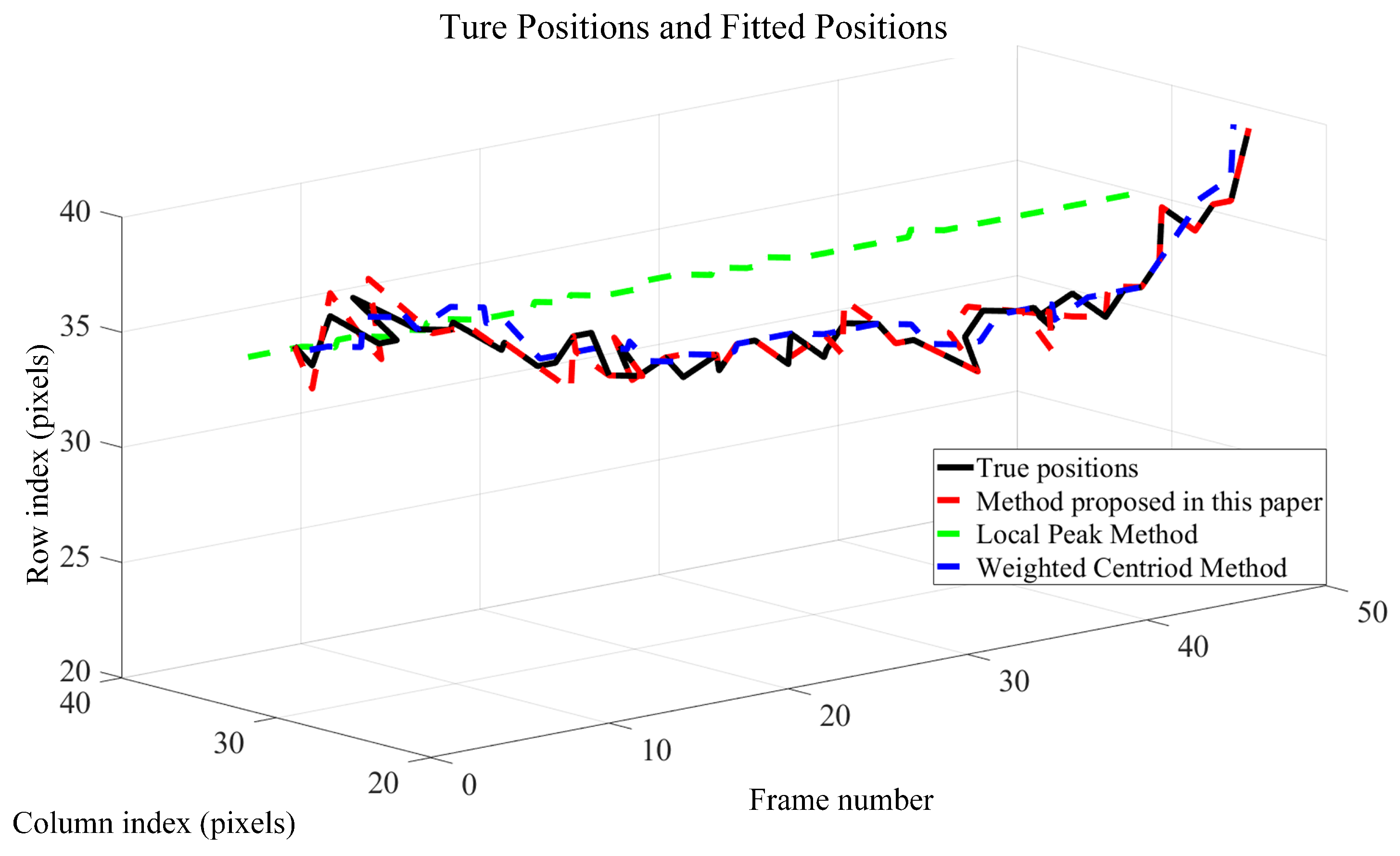
Therefore, in our experiments, three fitting methods were used to fit the multiframe UAV imaging results. Figure 8 shows the distribution of the calculated value and the actual value of the model’s center position.
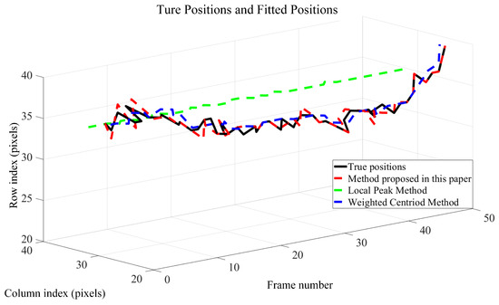
Figure 8.
Comparison of distribution between center position and model calculation position under different frame numbers.
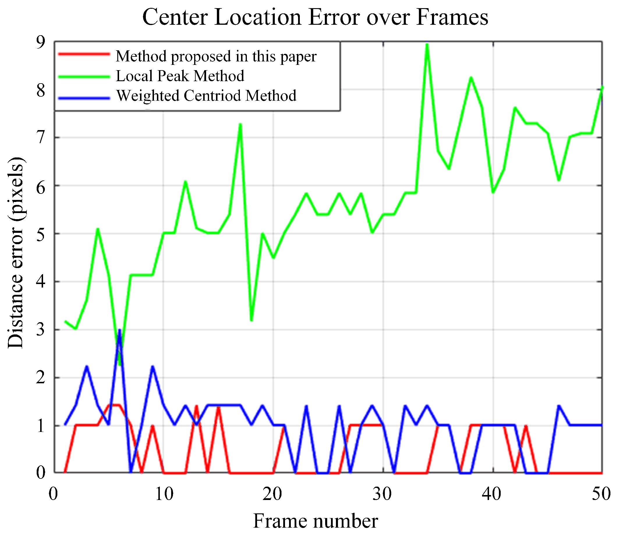
A comparison of the center positioning errors of different algorithms is shown in Figure 9, and the calculation results of MSE and R2 parameters are shown in Table 1. Due to the deviation of the maximum intensity of the target irradiated by laser, it is often the case that the local peak method leads to a large central error, high MSE, and negative R2, which shows that the fitting effect of this method on this dataset is very poor and can hardly explain the changing trend of the data. The centroid weighting method is easily influenced by noise, and its MSE value is high. When the noise is high, the position of the centroid may shift, resulting in the fitting result deviating from the true value and increasing CLE.
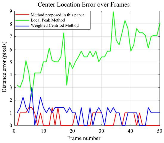
Figure 9.
Comparison of center positioning errors of different fitting methods under different frame numbers.

Table 1.
Comparison of quantitative indexes of different fitting methods.
In contrast, the fitting method proposed in Section 3.1 fully considers the influence of noise and outliers, and the central distribution error is less than 1, showing that this method has high accuracy in dealing with data migration. The R2 of the fitting is close to 1, which means that the fitting model can effectively capture the central variability of data, demonstrating the solid explanatory ability of the model to strengthen data. The MSE is 0.25, which shows that the deviation between the fitting result and the real value is minimal. These results further verify the accuracy and reliability of the proposed method in practical application.
4.2. Results of Tracking Algorithm for Gm-APD LiDAR System in Air and Space Background
In this section, the tracking performance of the Cam–Kalm algorithm proposed in Section 3.2 is compared with the Meanshift algorithm [64,65] and Camshift algorithm in terms of dynamic tracking.
The Meanshift algorithm is a simple nonparametric density estimation method. As a representative of matching search methods, it can be quickly applied to image processing, image classification, target recognition, and target tracking because of its advantages of small calculation, easy implementation, and certain adaptability [66,67]. Based on the Meanshift algorithm, target location and tracking are realized by iterative calculation of the mean vector. Because of the fast convergence of this algorithm, the target can be located quickly and effectively [68]. Our experiments used a DJI Elf 4 UAV with a flying distance of 70–100 m. The real UAV is shown in Figure 10, It has a size of 289.5 × 289.5 × 196 mm. The flight scene is shown in Figure 11.
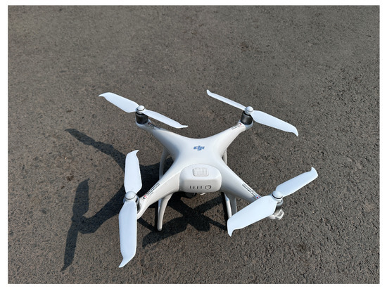
Figure 10.
Physical appearance of flying target.
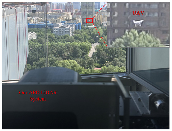
Figure 11.
Close-range tracking experimental scene.
The tracking results corresponding to the Cam–Kalm algorithm proposed in this paper are shown in Figure 12.
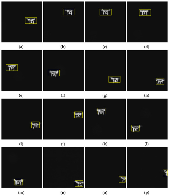
Figure 12.
Multiframe UAV dynamic tracking results of Gm-APD LiDAR based on Cam–Kalm algorithm in air and space background: (a) Frame 1; (b) Frame 33; (c) Frame 48; (d) Frame 52; (e) Frame 70; (f) Frame 86; (g) Frame 100; (h) Frame 114; (i) Frame 123; (j) Frame 133; (k) Frame 152; (l) Frame 179; (m) Frame 190; (n) Frame 199; (o) Frame 206; (p) Frame 215.
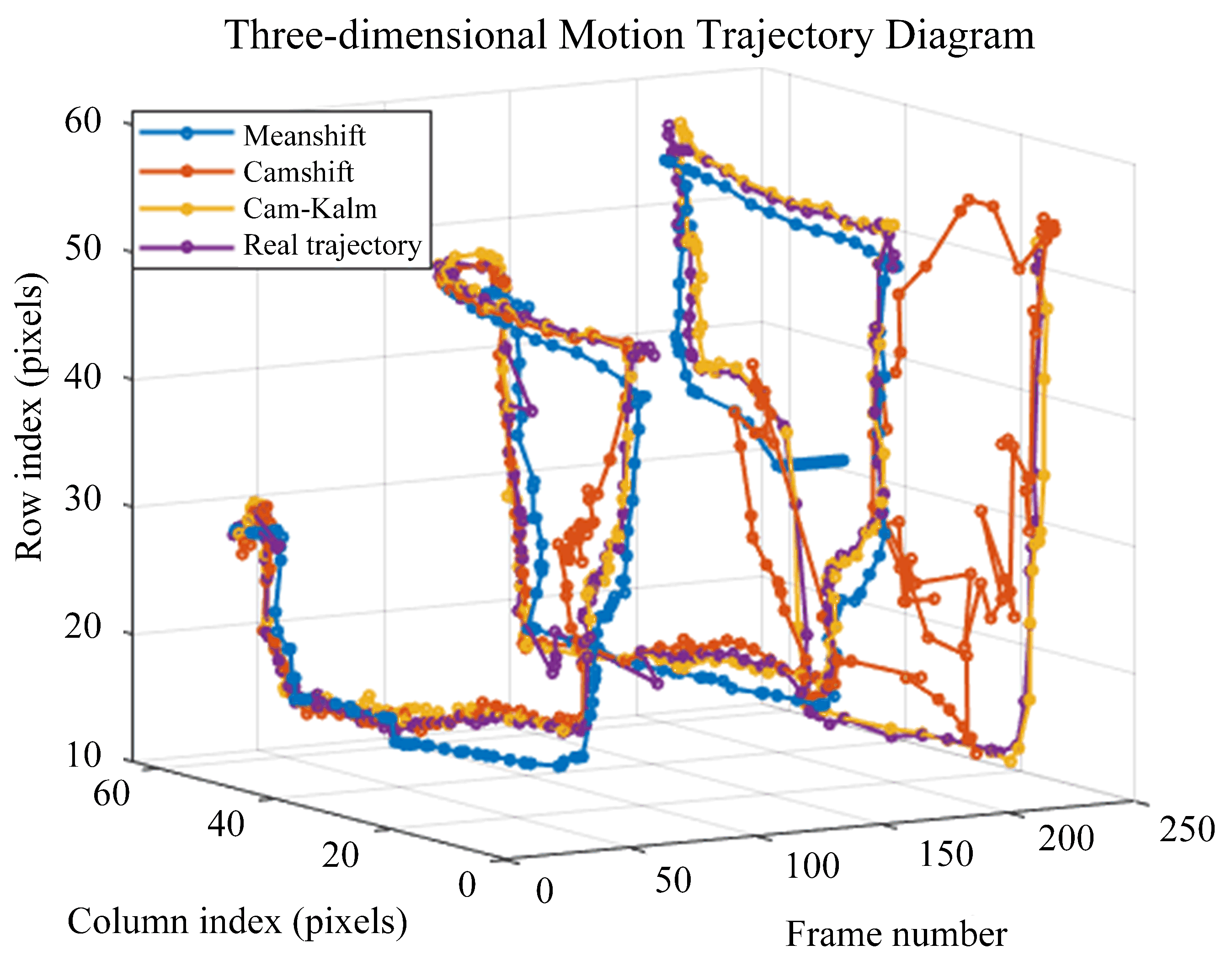
The fitting method proposed in Section 3.1 marks the point center of the imaging results. This method is used as the reference basis for the error calculation of the Camshift algorithm, Meanshift algorithm, and Cam–Kalm algorithm. These three algorithms were used to track the UAV. Figure 13 shows the multiframe tracking trajectory and the actual center trajectory of the marker.
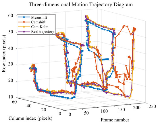
Figure 13.
Trajectory comparison using different tracking algorithms under multiple frames.
In Figure 13, the blue line shows the track of the tracking center provided by the Meanshift algorithm, the red line shows the trajectory of the tracking center of the Camshift algorithm, and the yellow line shows the trajectory of the tracking center of the Cam–Kalm algorithm, while the purple line is the actual trajectory of the target center obtained by fitting. The Meanshift algorithm tracks a target loss of around 215 frames, the Camshift algorithm tracks a target loss of around 160 frames, and the Cam–Kalm algorithm maintains stable tracking.
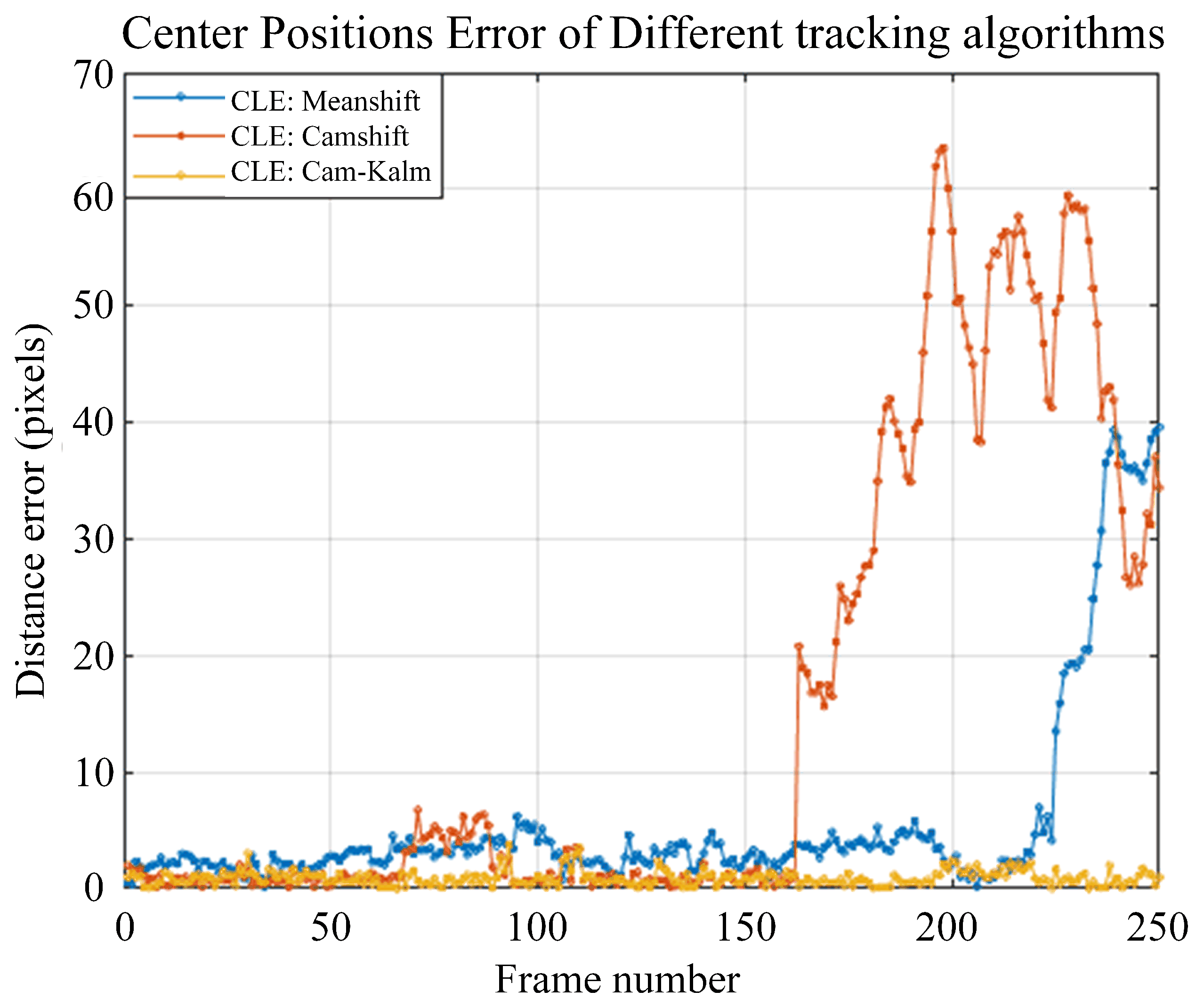
Figure 14 shows the calculated CLE of each frame when different tracking algorithms are used.

Figure 14.
Comparison of center positioning errors using different tracking algorithms under multiple frames.
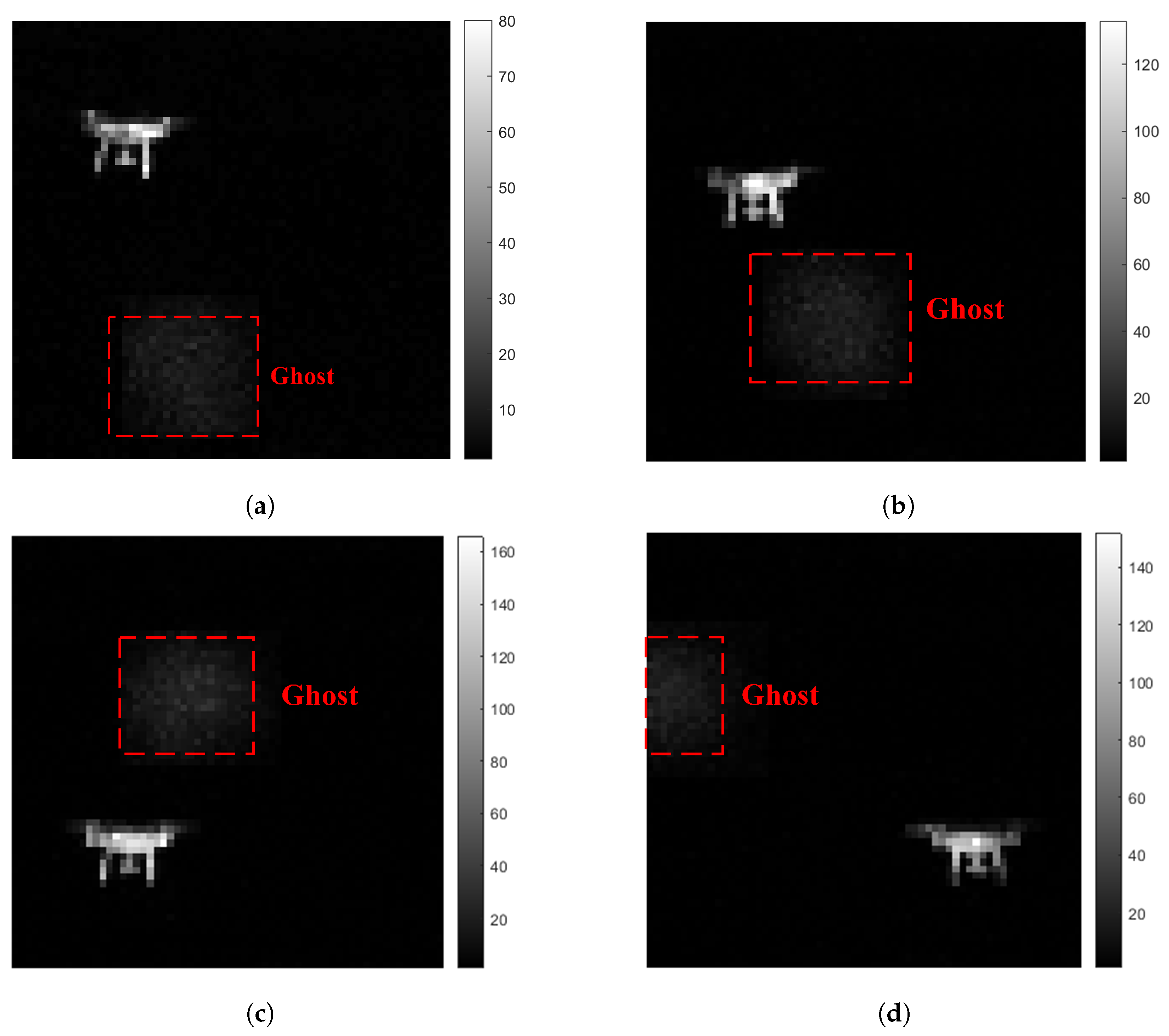
As can be seen in Figure 14, the Meanshift algorithm shows the biggest CLE between the 215th and 250th frames due to loss of the target. This is because the search window size of the Meanshift algorithm is fixed. When the target is at the edge of the field of view and the imaging size is less than half of the actual size, the algorithm cannot readjust the search window to capture the correct boundary of the target. Thus, the algorithm cannot track the target effectively, leading to tracking failure. The Camshift algorithm began to lose the target in the 162nd frame, which is attributed to a ghost phenomenon in the imaging results of this frame (shown in Figure 15). The algorithm mistakenly regarded the ghost as the real target, leading to tracking failure. In addition, when the moving speed of the target is too fast, the Meanshift and Camshift algorithms experience the phenomenon of tracking frame lag. As a result, both of these algorithms fail to effectively predict the target position from 67 frames to 89 frames, resulting in a sizable CLE.
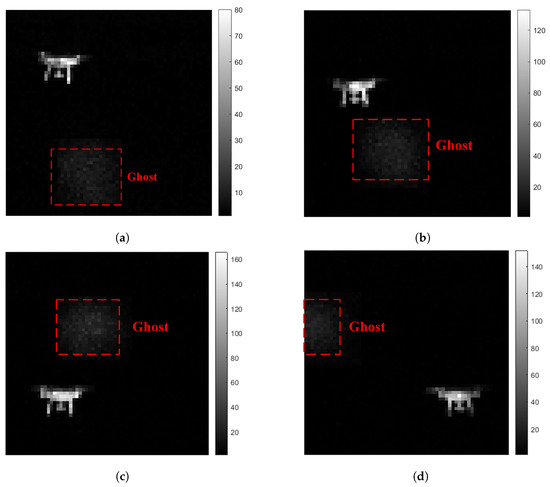
Figure 15.
Ghost phenomenon imaged by Gm-APD single-photon LiDAR: (a) intensity image of Frame 162, (b) intensity image of Frame 174, (c) intensity image of Frame 180, (d) intensity image of Frame 195.
In the tracking process of 250 frames, the Cam–Kalm algorithm proposed in this paper shows stable tracking performance. The Kalman filter smoothens the motion trajectory of the target and corrects the jitter caused by noise or incomplete imaging size in the tracking process, making the tracking more robust and continuous. At the same time, by modeling the speed and acceleration of the target, the Kalman filter can predict both the target’s position in the next frame. The effect is remarkable when the target suddenly accelerates or decelerates, and can maintain the continuity and accuracy of tracking. Especially in the vicinity of Frame 67, when the centroid of the target changes beyond the set confidence threshold, the Kalman filter is able to intervene and predict the position, thereby stabilizing the tracking process and avoiding tracking failure caused by motion state distortion. In addition, near the segment containing Frame 162, a ghost phenomenon appears due to the influence of the receiving optical lens of the Gm-APD LiDAR. Under this phenomenon the Camshift algorithm experiences tracking error, while the Cam–Kalm algorithm can predict the target position and model the target motion continuously between frames, which successfully eliminates the interference caused by ghosts and ensures the stability and accuracy of tracking.
Kalman filtering further narrows the search window of Camshift, improving the tracking efficiency and reducing the required computation. Kalman filters can deal with uniform motion as well as predict complex non-uniform motion such as acceleration changes of the target UAV, which makes the tracking effect more robust than using Camshift alone. Compared to the Meanshift and Camshift algorithms, the CLE of the proposed Cam–Kalm algorithm is always very low and its value is always less than 3 pixels. The average value of the multiframe CLE is 0.8964, which is less than a single pixel, and the variance is 0.4028, which shows the high tracking accuracy and stability of the proposed algorithm.
Therefore, the Cam–Kalm algorithm in this paper shows several apparent advantages in target tracking compared with the Meanshift and Camshift algorithms:
- Strong robustness: The Cam–Kalm algorithm can smooth the target’s trajectory by introducing a Kalman filter, correcting the jitter caused by noise or incomplete imaging and making the tracking more stable. This filter plays a particularly significant role when the target is subjected to rapid acceleration and deceleration, helping to maintain high tracking stability.
- Higher tracking accuracy: During the tracking process, the algorithm’s CLE is less than 3 pixels, the average CLE of multiple frames is 0.8964, and the variance is 0.4028, showing high accuracy and stability. In comparison, the values achieved with the Meanshift and Camshift algorithms are lower, indicating that the Cam–Kalm algorithm is superior in terms of tracking accuracy.
- Higher tracking efficiency: The traditional Meanshift and Camshift algorithms may need to be compared in the whole field of vision every time, which becomes significant when the target suddenly changes position or moves quickly, as this global search method will waste many computing resources. By using the Kalman filter to predict the trajectory of the target, the Cam–Kalm algorithm can effectively limit the search area to the vicinity of the prediction area and reduce the amount of invalid calculations. In this way, the algorithm can quickly find the target in a small range, leading to improved tracking efficiency.
- Dynamically adjustable tracking strategy: By setting the confidence threshold, the Cam–Kalm algorithm can flexibly choose different tracking strategies according to the changes in the centroid of the target. When the movement of the target changes considerably, such as in the case of acceleration or sudden change of direction, the algorithm can rely more on the prediction results of the Kalman filter, which is helpful for accurately predicting and updating the target position when the target moves quickly and avoiding tracking lag or failure caused by high speeds. This is especially important for fast-changing targets such as drones, and can ensure accurate tracking when the target is flying at high speed.
- –
- If the target changes little, such as moving at a constant speed, the algorithm is more inclined to trust the Camshift results. Camshift’s adaptability can help to track and locate the target more accurately.
- –
- If the target changes considerably, such as in the case of sudden acceleration, the Kalman filter’s prediction ability can help to reduce error and lag while ensuring tracking continuity.
The shortcomings of the proposed algorithm are as follows:
- Sensitivity to the centroid change setting: The confidence threshold set in the algorithm has an important influence on the results. This threshold determines how many pixels the centroid changes by. When the centroid changes by less than this threshold, the algorithm will believe the prediction result of the Kalman filter; when the centroid changes less than this threshold, the algorithm will rely on the Camshift prediction value. If the threshold is not set correctly, it may lead to tracking errors, especially when the target trajectory changes significantly, affecting the algorithm’s reliability.
- Reliance on accurate initial estimates: The Kalman filter relies on accurate initial position estimation. If the initial estimation is wrong, then the Kalman filter’s prediction may deviate from the actual target, affecting the subsequent tracking effect.
- Misjudgment: Although Camshift’s adaptive characteristics enable it to cope with changes in target size, the Kalman filter itself does not adapt to rapid changes in the target’s appearance, for example when the target is blocked. Thus, misjudgment may occur, especially in scenes where the imaging size changes significantly due to very complex scenes or the presence of rushing water.
4.3. Results of Tracking Algorithm for Gm-APD LiDAR System in Complex Background of Urban Buildings
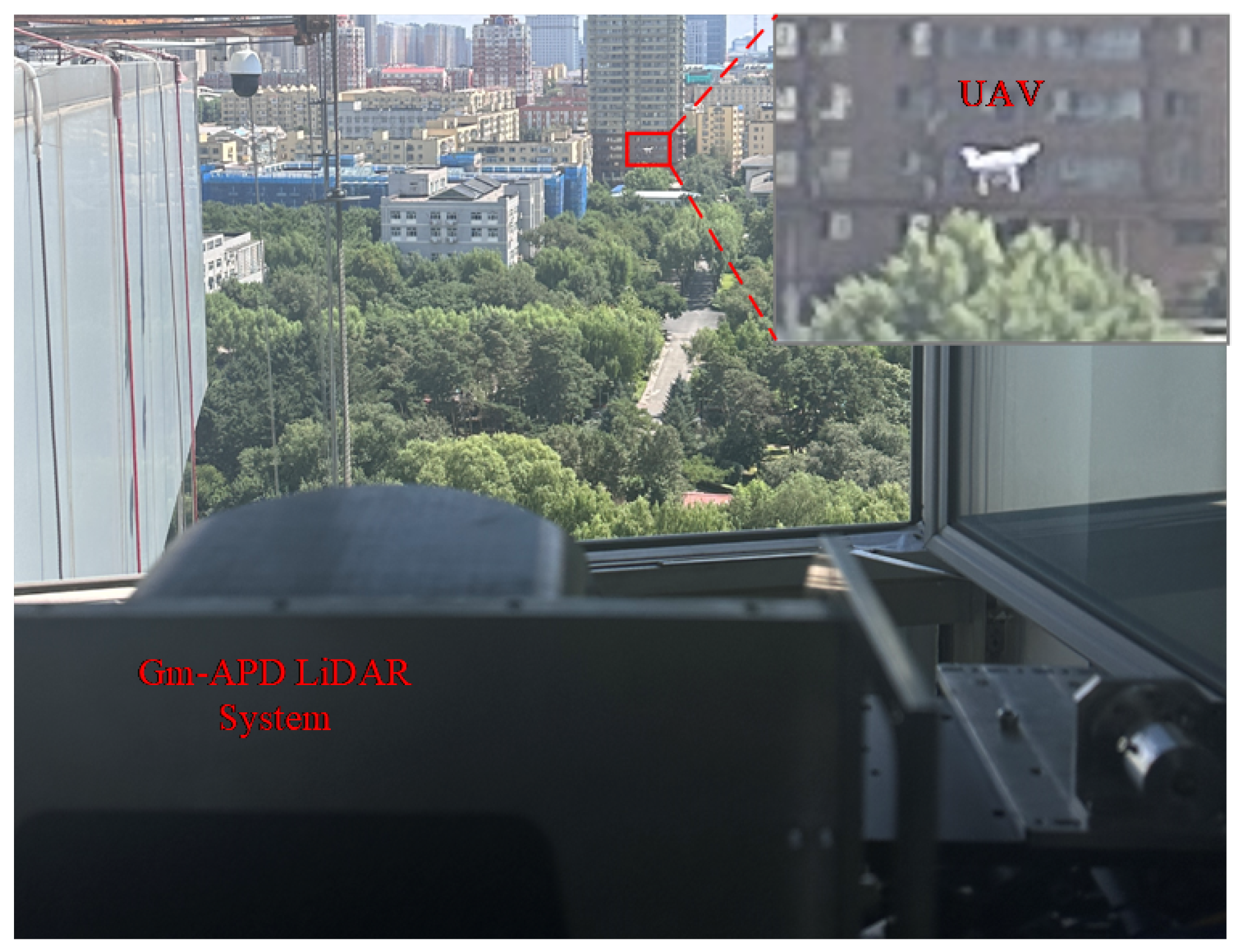
To further verify the tracking ability of the proposed Cam–Kalm algorithm for Gm-APD single-photon LiDARs in a complex scene, we switched the experimental environment from the aerospace background to a complex scene with urban buildings as the background. In this experiment, we reduced the field of view of Gm-APD single-photon LiDAR to 1° in order to track the DJI Elf 4 UAV more than 100 m away.
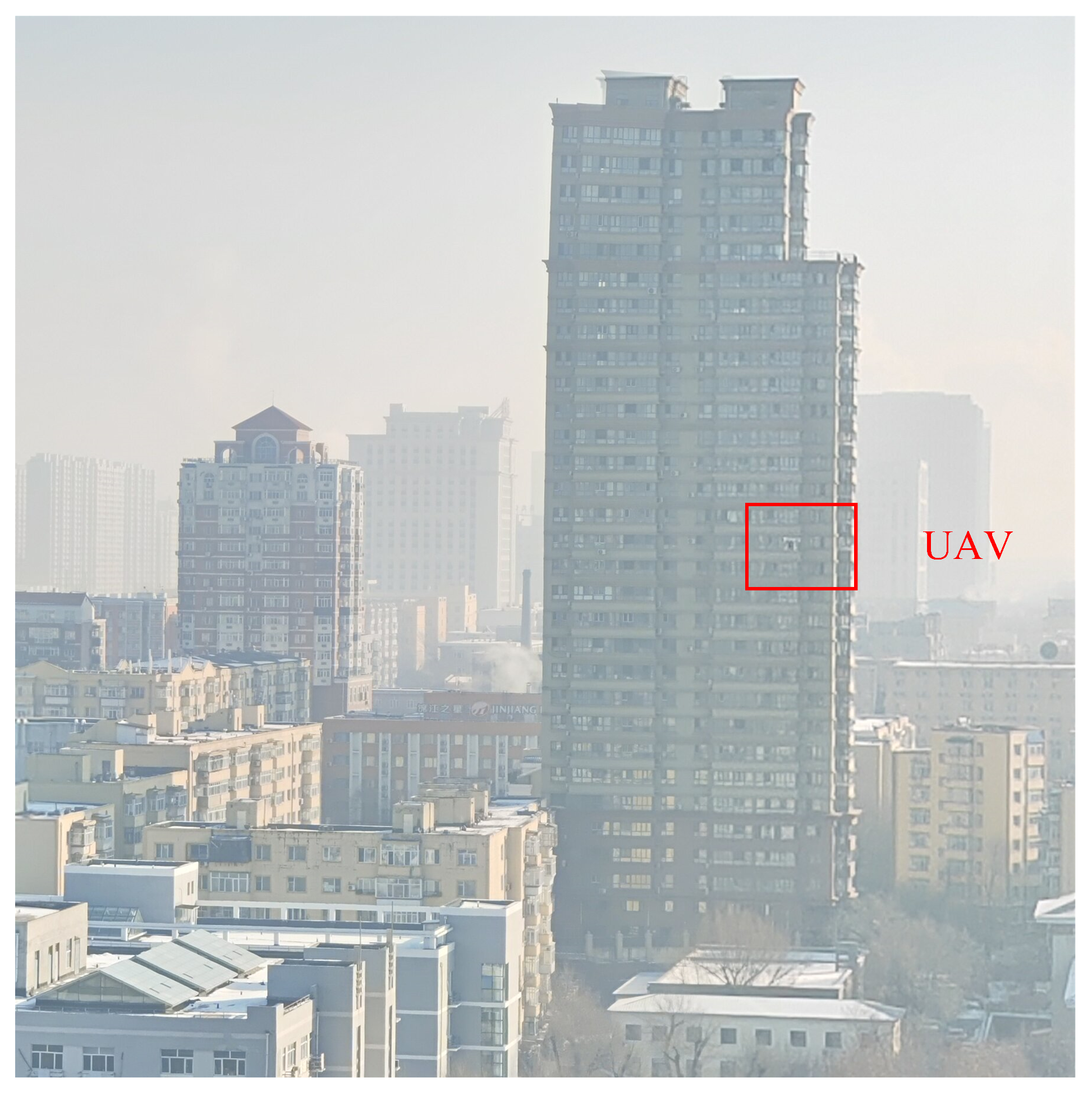
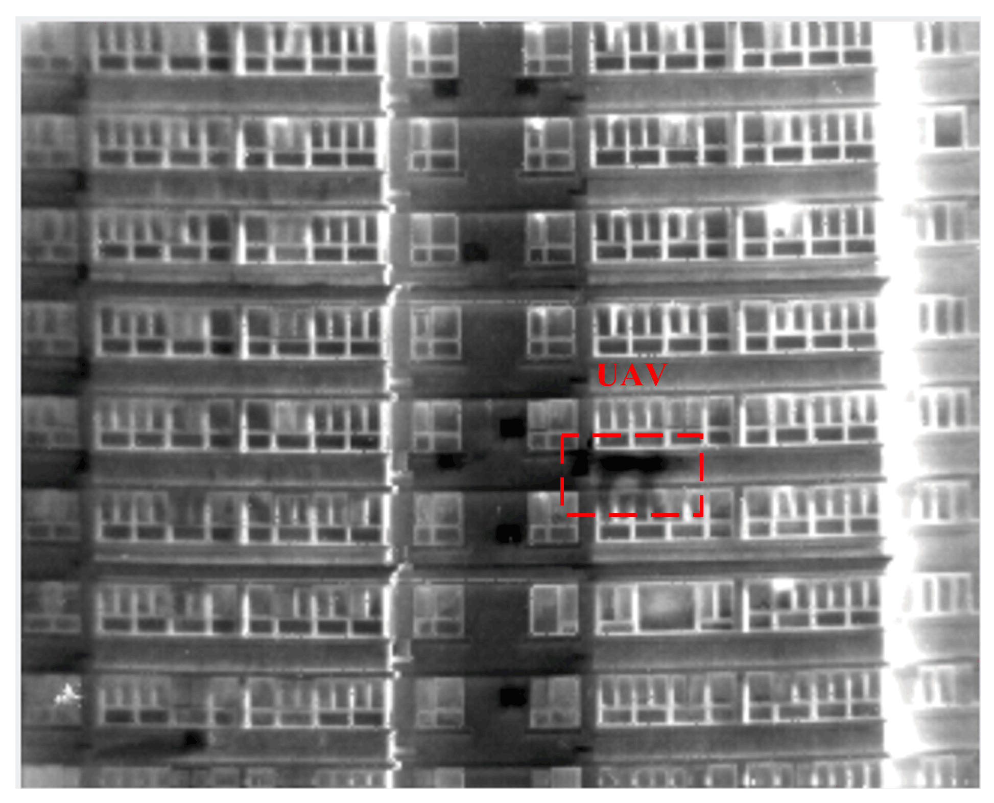
Figure 16 shows the experimental scene. The experiment was conducted in the morning, the weather was cloudy, and the visibility was less than 3 km). Figure 17 shows the imaging results of the infrared camera in the complex background.

Figure 16.
Experimental scene diagram of UAV flying against a complex background of urban buildings.

Figure 17.
Imaging results of UAV detected by infrared camera in the complex scene.
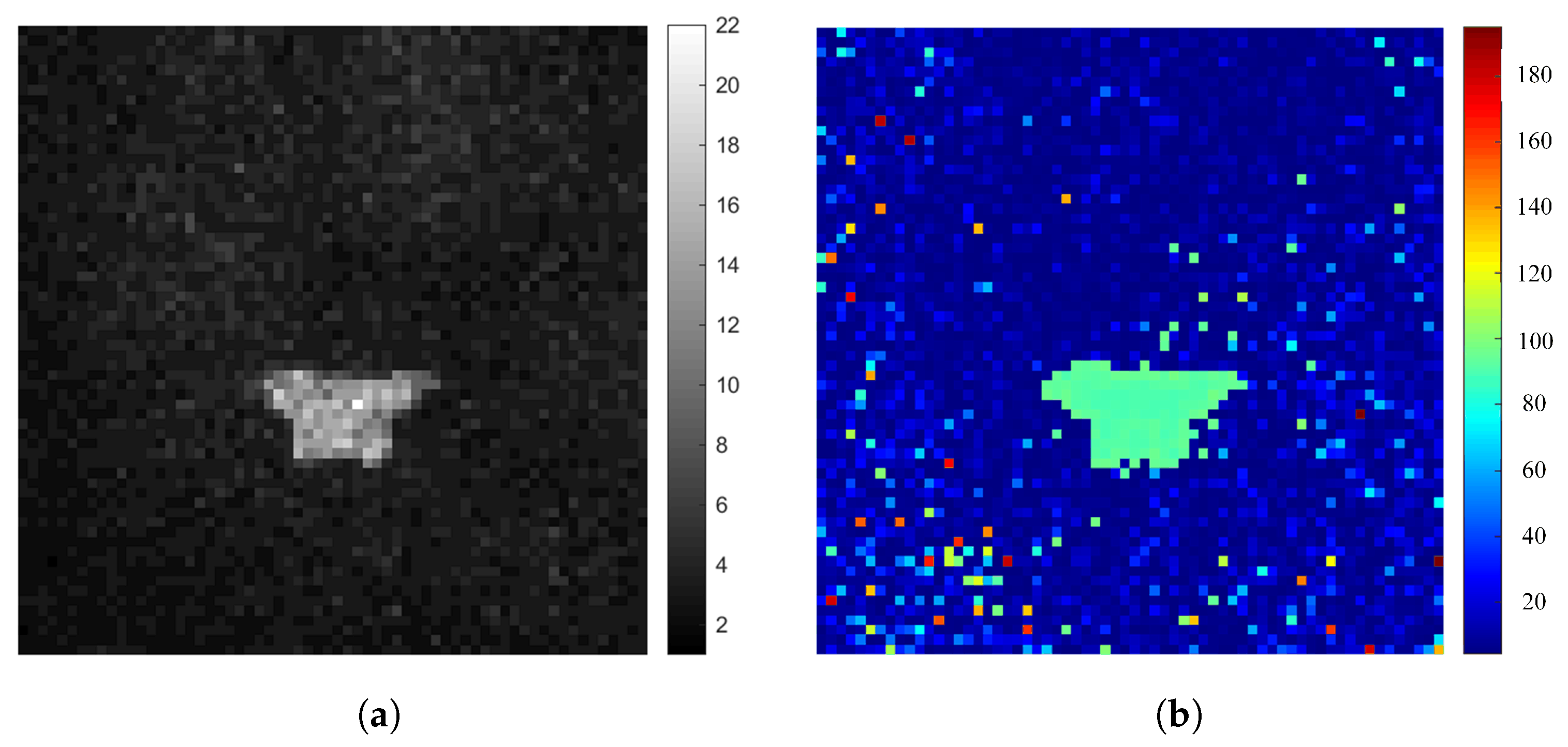
From the experimental scene shot by infrared camera, it can be seen that the background of urban buildings makes the UAV almost submerged by the environment. Under these conditions, it is difficult to extract the edge information effectively. Figure 18 shows the imaging results of a Gm-APD single-photon LiDAR against this complex background. Despite the complex environment, the Gm-APD single-photon LiDAR can detect UAV targets effectively.

Figure 18.
Imaging results showing the DJI Elf 4 UAV target obtained by the Gm-APD LiDAR in complex background conditions: (a) target intensity image and (b) target range image.
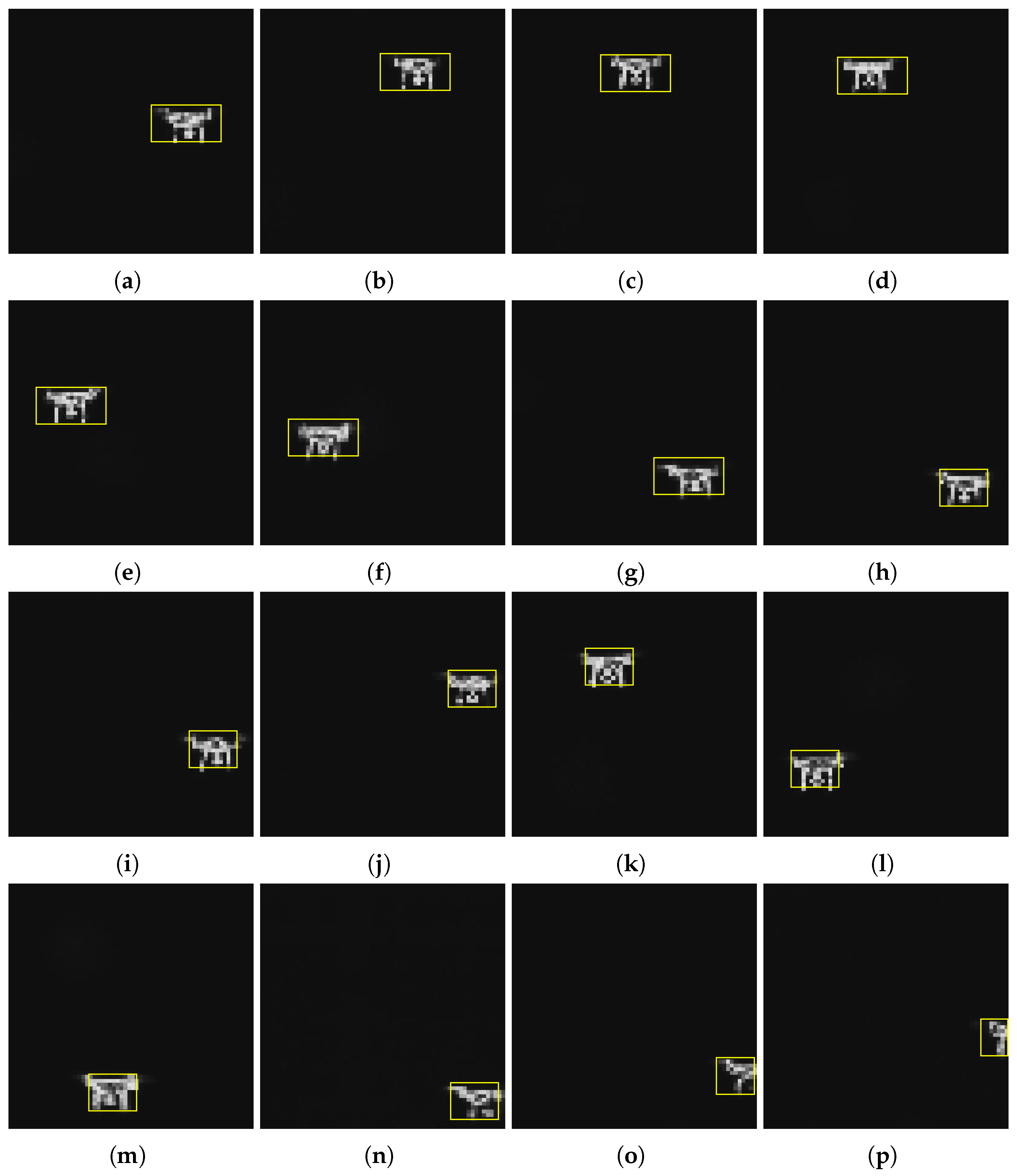
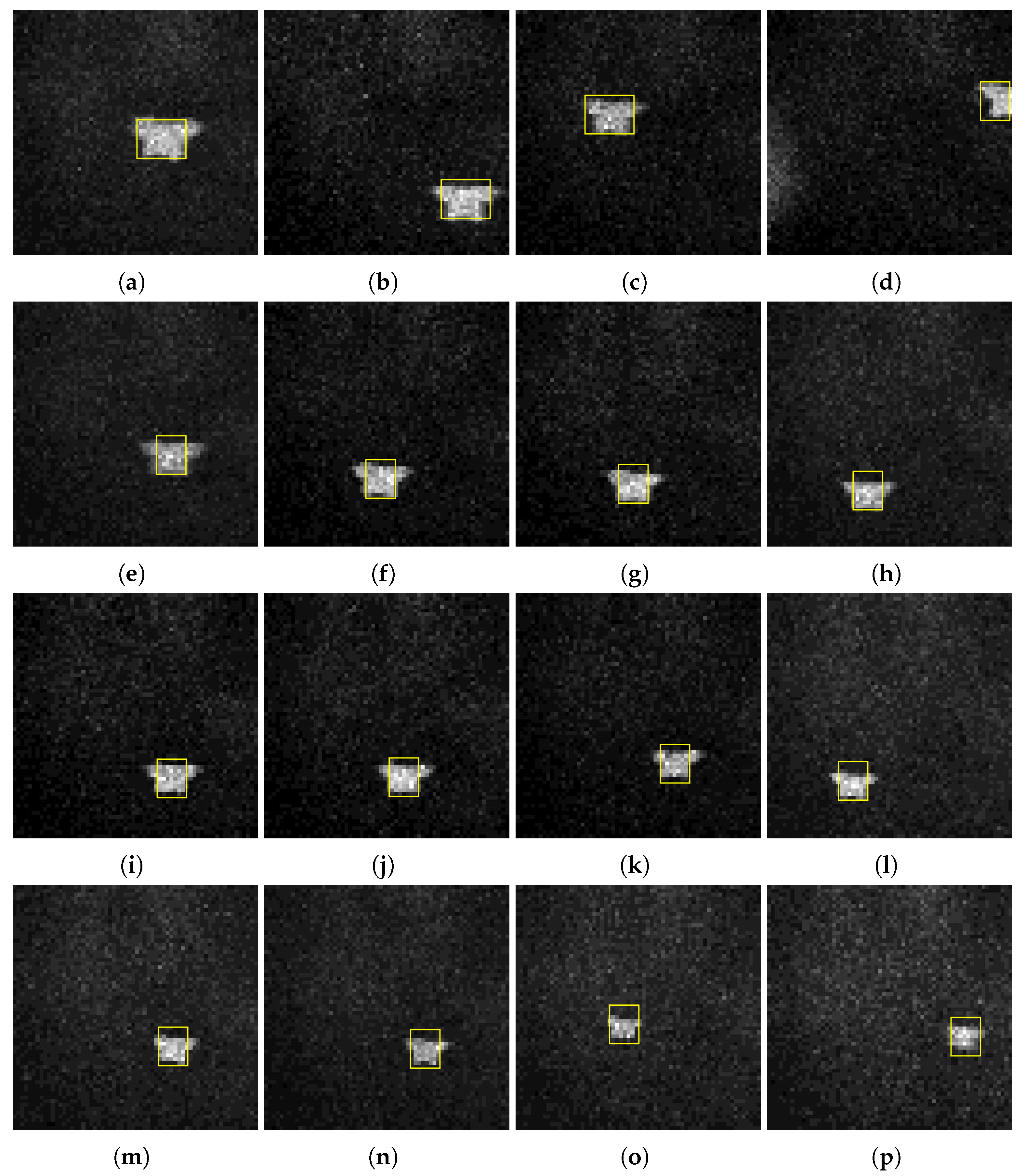
In this context, the Cam–Kalm tracking algorithm was applied to dynamically track the UAV in flight. The UAV was flying away from the single-photon LiDAR. During the tracking process of 600 frames, the Cam–Kalm algorithm maintained stable tracking. The tracking results are shown in Figure 19.
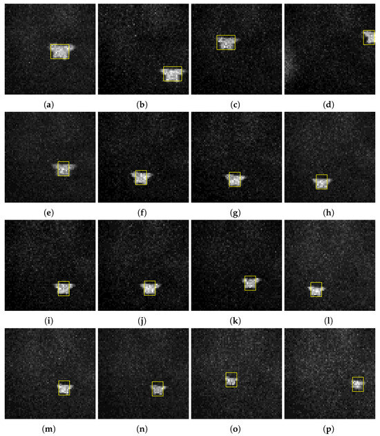
Figure 19.
Multiframe UAV dynamic tracking results of Gm-APD LiDAR based on Cam–Kalm algorithm in complex background: (a) Frame 001; (b) Frame 049; (c) Frame 085; (d) Frame 106; (e) Frame 168; (f) Frame 226; (g) Frame 280; (h) Frame 325; (i) Frame 354; (j) Frame 373; (k) Frame 420; (l) Frame 463; (m) Frame 507; (n) Frame 509; (o) Frame 587; (p) Frame 599.
Based on the reconstruction results of the single-photon LiDAR, we obtained the UAV’s flight trajectory, as shown in Figure 20. At the beginning of the experiment, the distance between the UAV and LiDAR was 101 m, while at the end the distance was 308 m. The effective and continuous tracking distance during the experiment was 207 m.
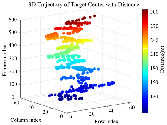
Figure 20.
Tracking trajectory of the Gm-APD LiDAR for the DJI Elf 4 UAV in complex background (smoothed).
The experimental results show that the Cam–Kalm algorithm tracked the UAV accurately and stably despite the complex background in the urban environment. This verifies the algorithm’s robustness in dynamic and crowded environments and shows its potential in practical applications. The results of the experiment in a complex scene further prove the algorithm’s adaptability, in particular the feasibility of target tracking in urban environments, and emphasize its prospects for application in the real world.
4.4. Long-Distance Tracking Results of Gm-APD LiDAR Based on Cam–Kalm Algorithm
To further realize long-distance target tracking, the FoV angle of the Gm-APD LiDAR imaging system was automatically adjusted to 0.06° according to the target distance. In this experiment, a MAVIC 3 UAV was used to complete a long-distance flight mission. The UAV is shown in Figure 21. This UAV’s fuselage size is 221 × 96.3 × 90.3 mm, and its deployed size is 347.5 × 283 × 107.7 mm. The size of this fuselage is the minimum detection size that can be resolved by a single pixel at a long distance. The maximum flight speed of the UAV in the experiment was 15 m/s and the maximum flight acceleration was 2 m/s2.
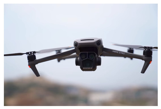
Figure 21.
Image of the UAV used in the long-distance flight experiment.
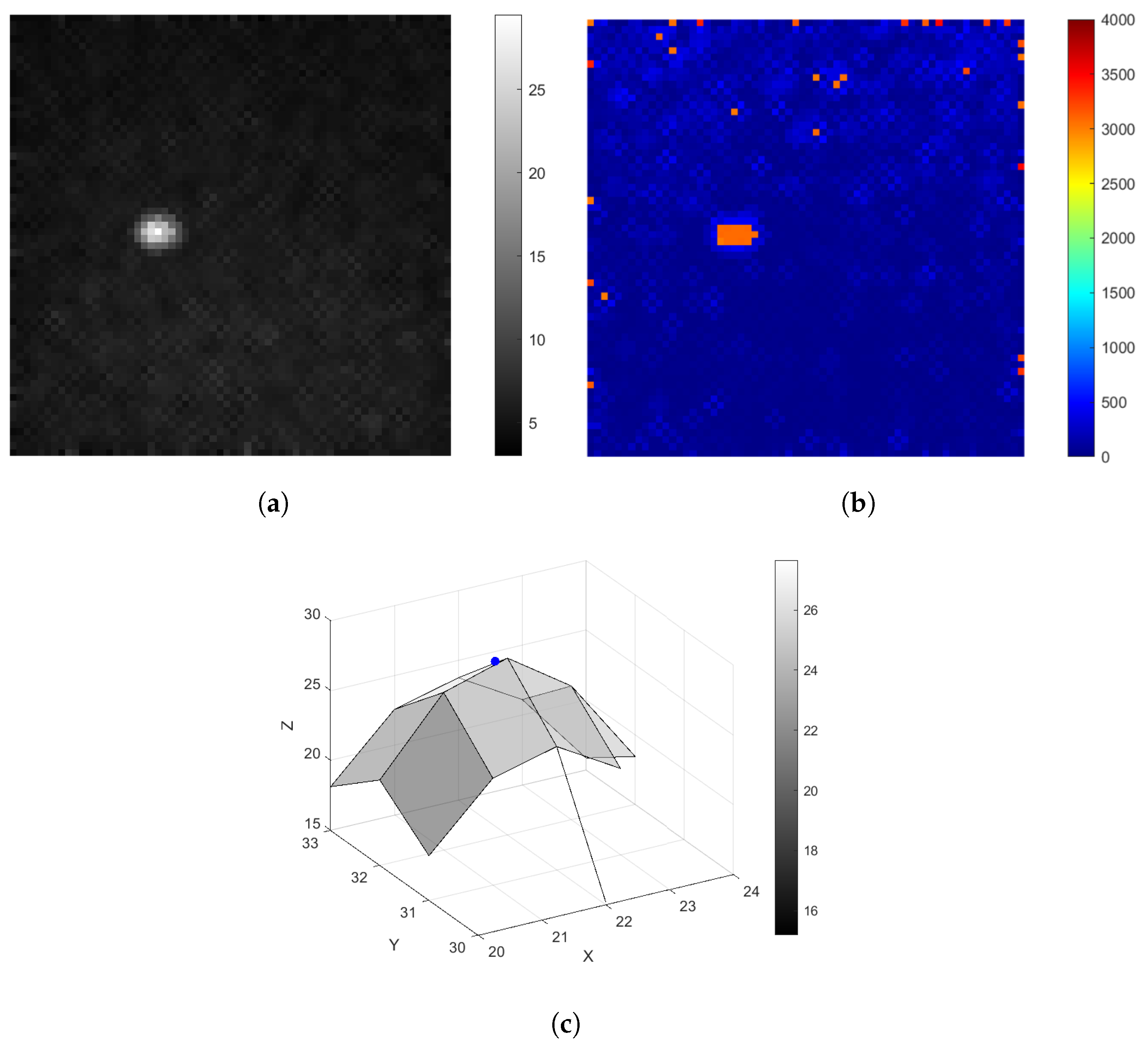
The Gm-APD LiDAR detected the MAVIC 3 UAV in 3 km airspace, and the imaging results of the system are shown in Figure 22a,b. The fitting distribution of the two-dimensional Gaussian model is shown in Figure 22c. The model’s corresponding MSE was 0.0909, and the R2 value was 0.9952.

Figure 22.
Reconstruction results and fitting distribution of the Gm-APD LiDAR for long-range detection of the the MAVIC 3 UAV: (a) target intensity image, (b) target range image, and (c) target fitting distribution.
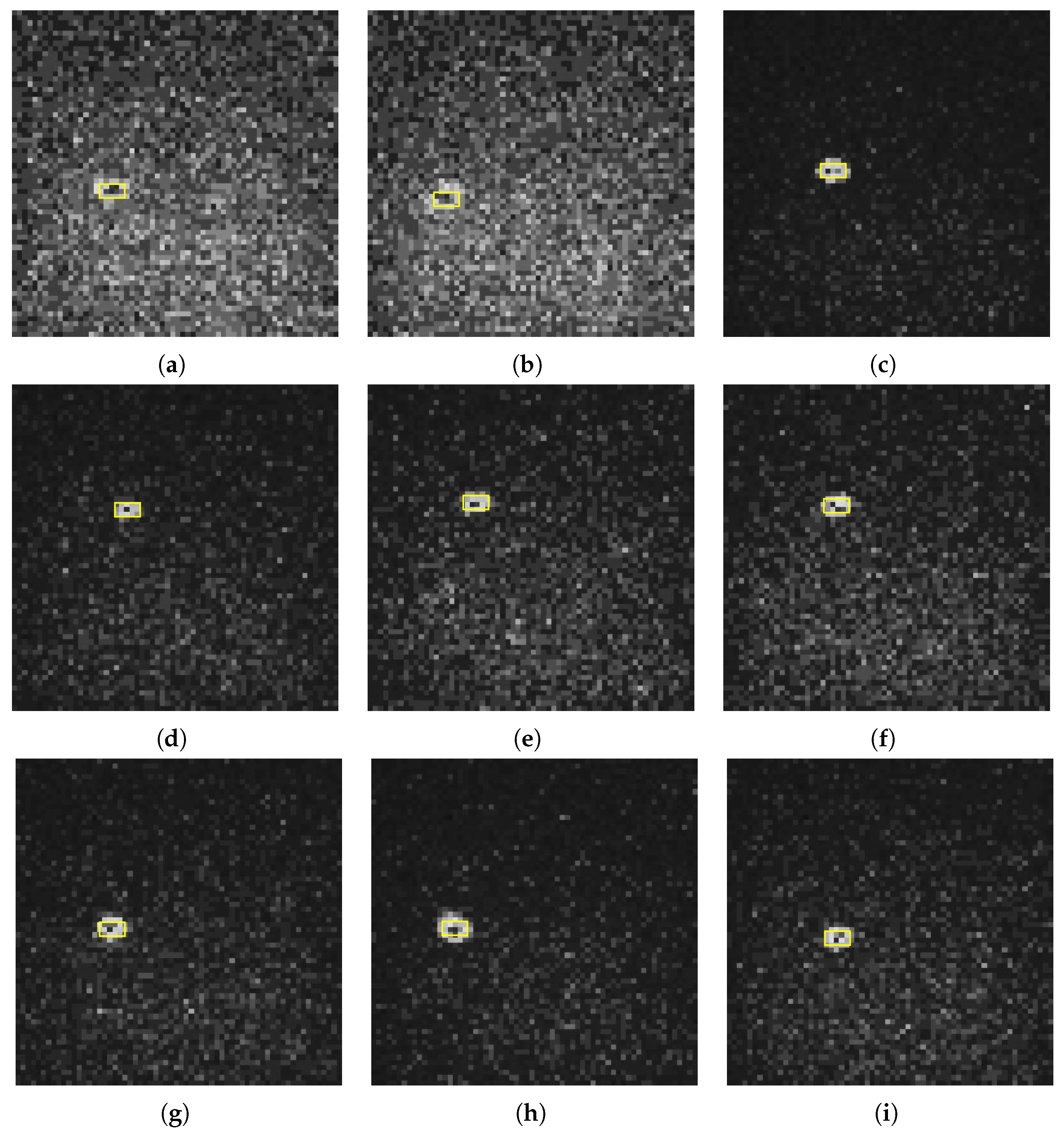
The corresponding tracking results of the Cam–Kalm tracking algorithm proposed in this paper are shown in Figure 23.
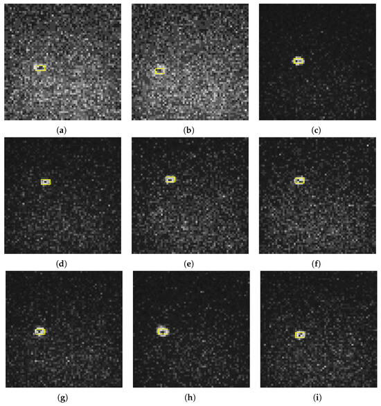
Figure 23.
Multiframe UAV dynamic tracking results at 3 km for the Gm-APD LiDAR based on the Cam–Kalm algorithm: (a) Frame 1; (b) Frame 9; (c) Frame 22; (d) Frame 31; (e) Frame 48; (f) Frame 59; (g) Frame 71; (h) Frame 85; (i) Frame 95.
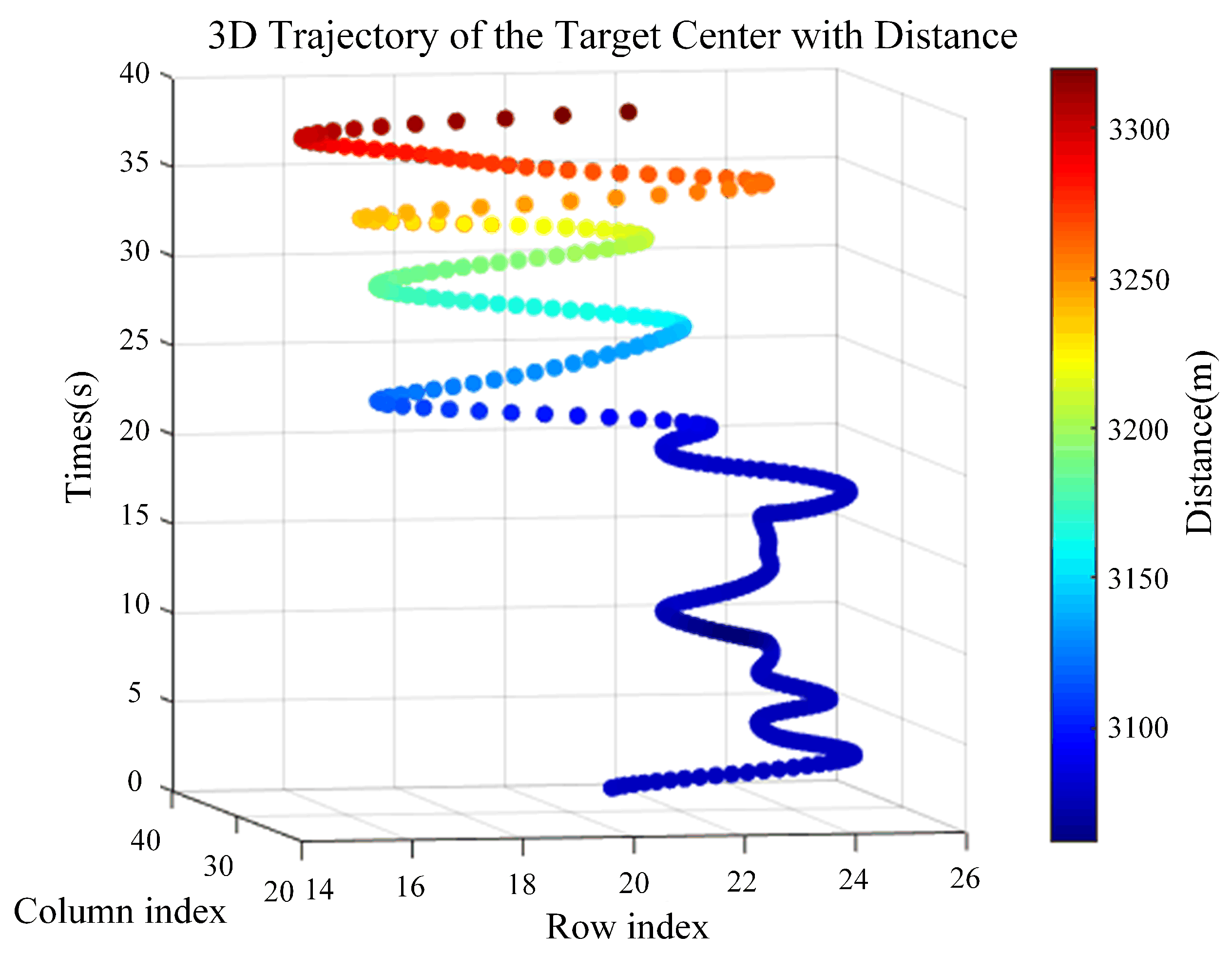
Using the Cam–Kalm algorithm, the Gm-APD LiDAR calculates the miss distance of the target according to the fitted centroid change. The frame rate of the tracking imaging in this experiment was 50 Hz, and the field of view angle of the LiDAR was adjusted for target tracking using the servo turntable. The space trajectory of the UAV target after smoothing is shown in Figure 24. During the tracking process, the initial distance of the target measured by the LiDAR was 3077.8 m, while at the end of tracking the target distance was 3320.3 m. The effective tracking distance was 242.5 m.

Figure 24.
Tracking trajectory of the Gm-APD LiDAR for the DJI MAVIC 3 UAV at long distance (smoothed).
5. Conclusions
In this paper, an automatic laser tracking and ranging system based on a Gm-APD LiDAR is designed and implemented, and we propose the Cam–Kalm algorithm combining a Kalman filter and the Camshift algorithm. This combination significantly improves the tracking accuracy and stability for small, low, and slow targets. The proposed system can independently determine the target’s center position and tracking frame by introducing a two-dimensional Gaussian fitting and edge detection algorithm, allowing it to realize automatic tracking. Our experimental results show that the proposed system not only demonstrates high fitting accuracy in the range of 70 m, but can also successfully track a UAV in real-time against a long-distance scene from 3.07 km to 3.32 km, which verifies its practicability in long-distance target detection.
This study provides a new solution based on single-photon LiDAR for UAV airspace early-warning technology, especially in long-distance tracking and ranging scenarios involving non-cooperative targets in airspace. However, early warning, detection, and attack of distributed drone swarm targets are still realistic problems that need urgent solving. Because single-photon LiDARs have a small FOV and only a single working mode, it is not possible to cope with a distributed drone swarm by relying only on the single-mode working form of the single-photon LiDAR. In future work, we plan to further explore and integrate data from other sensors, such as a visible light camera, short-wave infrared camera, phased-array radar, or 5G-A for composite detection as a way to improve the system’s multi-target tracking ability and better cope with challenges related to drone swarms. At the same time, we intend to further expand the non-cooperative target recognition ability of the single-photon LiDAR in the proposed system, realize real-time three-dimensional positioning and tracking of various types of UAVs, and further improve the operational effectiveness of UAV early warning systems.
Author Contributions
Conceptualization, D.G. and Y.Q.; methodology, Y.Q. and X.Z.; software, J.L. and F.L.; validation, Y.Q., D.G. and S.Y.; formal analysis, D.G.; investigation, J.L. and F.L.; resources, D.G.; data curation, J.S. and X.Z.; writing—original draft preparation, D.G.; writing—review and editing, Y.Q. and J.S.; visualization, X.Z.; supervision, Y.Q. and X.Z.; project administration, D.G.; funding acquisition, J.S. All authors have read and agreed to the published version of the manuscript.
Funding
This research received no external funding.
Data Availability Statement
The original contributions presented in the study are included in the article; further inquiries can be directed to the corresponding author.
Conflicts of Interest
Author Jie Lu and Feng Liu were employed by the company 44th Research Institute of China Electronics Technology Group Corporation. The remaining authors declare that the research was conducted in the absence of any commercial or financial relationships that could be construed as a potential conflict of interest.
References
- Farlík, J.; Gacho, L. Researching UAV threat–new challenges. In Proceedings of the 2021 International Conference on Military Technologies (ICMT), Brno, Czech Republic, 8–11 June 2021; IEEE: Piscataway, NJ, USA, 2021; pp. 1–6. [Google Scholar]
- Lyu, C.; Zhan, R. Global analysis of active defense technologies for unmanned aerial vehicle. IEEE Aerosp. Electron. Syst. Mag. 2022, 37, 6–31. [Google Scholar] [CrossRef]
- Zhou, Y.; Rao, B.; Wang, W. UAV swarm intelligence: Recent advances and future trends. IEEE Access 2020, 8, 183856–183878. [Google Scholar] [CrossRef]
- Mohsan, S.A.H.; Khan, M.A.; Noor, F.; Ullah, I.; Alsharif, M.H. Towards the unmanned aerial vehicles (UAVs): A comprehensive review. Drones 2022, 6, 147. [Google Scholar] [CrossRef]
- Peri, D. Expanding anti-UAVs market to counter drone technology. CLAWS J. Winter 2015, 152–158. [Google Scholar]
- Kang, H.; Joung, J.; Kim, J.; Kang, J.; Cho, Y.S. Protect your sky: A survey of counter unmanned aerial vehicle systems. IEEE Access 2020, 8, 168671–168710. [Google Scholar] [CrossRef]
- Liu, S.; Wu, R.; Qu, J.; Li, Y. HDA-Net: Hybrid convolutional neural networks for small objects recognization at airports. IEEE Trans. Instrum. Meas. 2022, 71, 2521314. [Google Scholar] [CrossRef]
- Solodov, A.; Williams, A.; Al Hanaei, S.; Goddard, B. Analyzing the threat of unmanned aerial vehicles (UAV) to nuclear facilities. Secur. J. 2018, 31, 305–324. [Google Scholar] [CrossRef]
- Taneski, N.; Caminski, B.; Petrovski, A. Use of weaponized unmanned aerial vehicles (UAVs) supported by gis as a growing terrorist threat. In Science and Society Contribution of Humanities and Social Sciences: Proceedings of the International Conference on the Occasion of the Centennial Anniversary of the Faculty of Philosophy, Struga, North Macedonia, 2–5 September 2020; Faculty of Philosophy: Skopje, North Macedonia, 2021; pp. 553–567. [Google Scholar]
- Wang, J.; Liu, Y.; Song, H. Counter-unmanned aircraft system (s)(C-UAS): State of the art, challenges, and future trends. IEEE Aerosp. Electron. Syst. Mag. 2021, 36, 4–29. [Google Scholar] [CrossRef]
- Wang, L.; Luo, J.; Li, Z.; Wang, M.; Li, R.; Xu, W.; He, F.; Xu, B. Thinking about anti-drone strategies. In Proceedings of the 2024 3rd International Conference on Artificial Intelligence, Internet of Things and Cloud Computing Technology (AIoTC), Wuhan, China, 13–15 September 2024; IEEE: Piscataway, NJ, USA, 2024; pp. 53–56. [Google Scholar]
- Anil, A.; Hennemann, A.; Kimmel, H.; Mayer, C.; Müller, L.; Reischl, T. PERSEUS-Post-Emergency Response and Surveillance UAV System; Deutsche Gesellschaft für Luft-und Raumfahrt-Lilienthal-Oberth eV: Bonn, Germany, 2024. [Google Scholar]
- Bi, Z.; Chen, H.; Hu, J.; Liu, L.; Yang, J.; Bai, C. Analysis of UAV Typical War Cases and Combat Assessment Research. In Proceedings of the 2022 IEEE International Conference on Unmanned Systems (ICUS), Guangzhou, China, 28–30 October 2022; IEEE: Piscataway, NJ, USA, 2022; pp. 1449–1453. [Google Scholar]
- Gong, J.; Yan, J.; Kong, D.; Li, D. Introduction to Drone Detection Radar with Emphasis on Automatic Target Recognition (ATR) technology. arXiv 2023, arXiv:2307.10326. [Google Scholar]
- Bressler, M.S.; Bressler, L. Beware the unfriendly skies: How drones are being used as the latest weapon in cybercrime. J. Technol. Res. 2016, 7, 1–12. [Google Scholar]
- Kim, E.; Sivits, K. Blended secondary surveillance radar solutions to improve air traffic surveillance. Aerosp. Sci. Technol. 2015, 45, 203–208. [Google Scholar] [CrossRef]
- Zmysłowski, D.; Skokowski, P.; Kelner, J.M. Anti-drone sensors, effectors, and systems–a concise overview. TransNav Int. J. Mar. Navig. Saf. Sea Transp. 2023, 17, 455–461. [Google Scholar] [CrossRef]
- Herrera, G.J.; Dechant, J.A.; Green, E.; Klein, E.A. Technology Trends in Small Unmanned Aircraft Systems (sUAS) and Counter-UAS: A Five-Year Outlook; Institute for Defense Analyses: Alexandria, VA, USA, 2022. [Google Scholar]
- Lykou, G.; Moustakas, D.; Gritzalis, D. Defending airports from UAS: A survey on cyber-attacks and counter-drone sensing technologies. Sensors 2020, 20, 3537. [Google Scholar] [CrossRef] [PubMed]
- Park, S.; Kim, H.T.; Lee, S.; Joo, H.; Kim, H. Survey on anti-drone systems: Components, designs, and challenges. IEEE Access 2021, 9, 42635–42659. [Google Scholar] [CrossRef]
- McManamon, P.F. Review of ladar: A historic, yet emerging, sensor technology with rich phenomenology. Opt. Eng. 2012, 51, 060901. [Google Scholar] [CrossRef]
- Becker, W.; Bergmann, A. Multi-dimensional time-correlated single photon counting. In Reviews in Fluorescence 2005; Springer: Boston, MA, USA, 2005; pp. 77–108. [Google Scholar]
- Prochazka, I.; Hamal, K.; Sopko, B. Recent achievements in single photon detectors and their applications. J. Mod. Opt. 2004, 51, 1289–1313. [Google Scholar] [CrossRef]
- Yuan, Z.; Kardynal, B.; Sharpe, A.; Shields, A. High speed single photon detection in the near infrared. Appl. Phys. Lett. 2007, 91, 041114. [Google Scholar] [CrossRef]
- Buller, G.; Collins, R. Single-photon generation and detection. Meas. Sci. Technol. 2009, 21, 012002. [Google Scholar] [CrossRef]
- Eisaman, M.D.; Fan, J.; Migdall, A.; Polyakov, S.V. Invited review article: Single-photon sources and detectors. Rev. Sci. Instrum. 2011, 82, 071101. [Google Scholar] [CrossRef]
- Fersch, T.; Weigel, R.; Koelpin, A. Challenges in miniaturized automotive long-range lidar system design. In Proceedings of the Three-Dimensional Imaging, Visualization, and Display 2017, Anaheim, CA, USA, 9–13 April 2017; SPIE: Bellingham, WA, USA, 2017; Volume 10219, pp. 160–171. [Google Scholar]
- Raj, T.; Hanim Hashim, F.; Baseri Huddin, A.; Ibrahim, M.F.; Hussain, A. A survey on LiDAR scanning mechanisms. Electronics 2020, 9, 741. [Google Scholar] [CrossRef]
- Pfeifer, N.; Briese, C. Laser scanning–principles and applications. In Proceedings of the Geosiberia 2007—International Exhibition and Scientific Congress, Novosibirsk, Russia, 25 April 2007; European Association of Geoscientists & Engineers: Bunnik, The Netherlands, 2007; pp. cp–59. [Google Scholar]
- Kim, B.H.; Khan, D.; Bohak, C.; Choi, W.; Lee, H.J.; Kim, M.Y. V-RBNN based small drone detection in augmented datasets for 3D LADAR system. Sensors 2018, 18, 3825. [Google Scholar] [CrossRef] [PubMed]
- Chen, Z.; Liu, B.; Guo, G. Adaptive single photon detection under fluctuating background noise. Opt. Express 2020, 28, 30199–30209. [Google Scholar] [CrossRef] [PubMed]
- Pfennigbauer, M.; Möbius, B.; do Carmo, J.P. Echo digitizing imaging lidar for rendezvous and docking. In Proceedings of the Laser Radar Technology and Applications XIV, Orlando, FL, USA, 13–17 April 2009; SPIE: Bellingham, WA, USA, 2009; Volume 7323, pp. 9–17. [Google Scholar]
- McCarthy, A.; Ren, X.; Della Frera, A.; Gemmell, N.R.; Krichel, N.J.; Scarcella, C.; Ruggeri, A.; Tosi, A.; Buller, G.S. Kilometer-range depth imaging at 1550 nm wavelength using an InGaAs/InP single-photon avalanche diode detector. Opt. Express 2013, 21, 22098–22113. [Google Scholar] [CrossRef] [PubMed]
- Pawlikowska, A.M.; Halimi, A.; Lamb, R.A.; Buller, G.S. Single-photon three-dimensional imaging at up to 10 kilometers range. Opt. Express 2017, 25, 11919–11931. [Google Scholar] [CrossRef] [PubMed]
- Zhou, H.; He, Y.; You, L.; Chen, S.; Zhang, W.; Wu, J.; Wang, Z.; Xie, X. Few-photon imaging at 1550 nm using a low-timing-jitter superconducting nanowire single-photon detector. Opt. Express 2015, 23, 14603–14611. [Google Scholar] [CrossRef]
- Liu, B.; Yu, Y.; Chen, Z.; Han, W. True random coded photon counting Lidar. Opto-Electron. Adv. 2020, 3, 190044. [Google Scholar] [CrossRef]
- Li, Z.P.; Ye, J.T.; Huang, X.; Jiang, P.Y.; Cao, Y.; Hong, Y.; Yu, C.; Zhang, J.; Zhang, Q.; Peng, C.Z.; et al. Single-photon imaging over 200 km. Optica 2021, 8, 344–349. [Google Scholar] [CrossRef]
- Kirmani, A.; Venkatraman, D.; Shin, D.; Colaço, A.; Wong, F.N.; Shapiro, J.H.; Goyal, V.K. First-photon imaging. Science 2014, 343, 58–61. [Google Scholar] [CrossRef]
- Hua, K.; Liu, B.; Chen, Z.; Wang, H.; Fang, L.; Jiang, Y. Fast photon-counting imaging with low acquisition time method. IEEE Photonics J. 2021, 13, 7800312. [Google Scholar] [CrossRef]
- Chen, Z.; Liu, B.; Guo, G.; He, C. Single photon imaging with multi-scale time resolution. Opt. Express 2022, 30, 15895–15904. [Google Scholar] [CrossRef]
- Ding, Y.; Qu, Y.; Zhang, Q.; Tong, J.; Yang, X.; Sun, J. Research on UAV detection technology of Gm-APD Lidar based on YOLO model. In Proceedings of the 2021 IEEE International Conference on Unmanned Systems (ICUS), Beijing, China, 15–17 October 2021; IEEE: Piscataway, NJ, USA, 2021; pp. 105–109. [Google Scholar]
- Zhou, X.; Sun, J.; Jiang, P.; Qiu, C.; Wang, Q. Improvement of detection probability and ranging performance of Gm-APD LiDAR with spatial correlation and adaptive adjustment of the aperture diameter. Opt. Lasers Eng. 2021, 138, 106452. [Google Scholar] [CrossRef]
- Alspach, D.L. A Gaussian sum approach to the multi-target identification-tracking problem. Automatica 1975, 11, 285–296. [Google Scholar] [CrossRef]
- Simon, D. Kalman filtering. Embed. Syst. Program. 2001, 14, 72–79. [Google Scholar]
- Exner, D.; Bruns, E.; Kurz, D.; Grundhöfer, A.; Bimber, O. Fast and robust CAMShift tracking. In Proceedings of the 2010 IEEE Computer Society Conference on Computer Vision and Pattern Recognition-Workshops, San Francisco, CA, USA, 13–18 June 2010; IEEE: Piscataway, NJ, USA, 2010; pp. 9–16. [Google Scholar]
- Bi, H.; Ma, J.; Wang, F. An improved particle filter algorithm based on ensemble Kalman filter and Markov chain Monte Carlo method. IEEE J. Sel. Top. Appl. Earth Obs. Remote Sens. 2014, 8, 447–459. [Google Scholar] [CrossRef]
- Kulkarni, M.; Wadekar, P.; Dagale, H. Block division based camshift algorithm for real-time object tracking using distributed smart cameras. In Proceedings of the 2013 IEEE International Symposium on Multimedia, Anaheim, CA, USA, 9–11 December 2013; IEEE: Piscataway, NJ, USA, 2013; pp. 292–296. [Google Scholar]
- Yang, P. Efficient particle filter algorithm for ultrasonic sensor-based 2D range-only simultaneous localisation and mapping application. IET Wirel. Sens. Syst. 2012, 2, 394–401. [Google Scholar] [CrossRef]
- Cong, D.; Shi, P.; Zhou, D. An improved camshift algorithm based on RGB histogram equalization. In Proceedings of the 2014 7th International Congress on Image and Signal Processing, Dalian, China, 14–16 October 2014; IEEE: Piscataway, NJ, USA, 2014; pp. 426–430. [Google Scholar]
- Xu, X.; Zhang, H.; Luo, M.; Tan, Z.; Zhang, M.; Yang, H.; Li, Z. Research on target echo characteristics and ranging accuracy for laser radar. Infrared Phys. Technol. 2019, 96, 330–339. [Google Scholar] [CrossRef]
- Chauve, A.; Mallet, C.; Bretar, F.; Durrieu, S.; Deseilligny, M.P.; Puech, W. Processing full-waveform lidar data: Modelling raw signals. Int. Arch. Photogramm. Remote Sens. Spat. Inf. Sci. 2007, 36, W52. [Google Scholar]
- Laurenzis, M.; Bacher, E.; Christnacher, F. Measuring laser reflection cross-sections of small unmanned aerial vehicles for laser detection, ranging and tracking. In Proceedings of the Laser Radar Technology and Applications XXII, Anaheim, CA, USA, 9–13 April 2017; SPIE: Bellingham, WA, USA, 2017; Volume 10191, pp. 74–82. [Google Scholar]
- Zhang, Y. Detection and tracking of human motion targets in video images based on camshift algorithms. IEEE Sens. J. 2019, 20, 11887–11893. [Google Scholar] [CrossRef]
- Bankar, R.; Salankar, S. Improvement of head gesture recognition using camshift based face tracking with UKF. In Proceedings of the 2019 9th International Conference on Emerging Trends in Engineering and Technology-Signal and Information Processing (ICETET-SIP-19), Nagpur, India, 1–2 November 2019; IEEE: Piscataway, NJ, USA, 2019; pp. 1–5. [Google Scholar]
- Vincent, L. Morphological area openings and closings for grey-scale images. In Shape in Picture: Mathematical Description of Shape in Grey-Level Images; Springer: Berlin/Heidelberg, Germany, 1994; pp. 197–208. [Google Scholar]
- Nishiguchi, K.I.; Kobayashi, M.; Ichikawa, A. Small target detection from image sequences using recursive max filter. In Proceedings of the Signal and Data Processing of Small Targets 1995, San Diego, CA, USA, 9–14 July 1995; SPIE: Bellingham, WA, USA, 1995; Volume 2561, pp. 153–166. [Google Scholar]
- Rong, W.; Li, Z.; Zhang, W.; Sun, L. An improved CANNY edge detection algorithm. In Proceedings of the 2014 IEEE International Conference on Mechatronics and Automation, Tianjin, China, 3–6 August 2014; IEEE: Piscataway, NJ, USA, 2014; pp. 577–582. [Google Scholar]
- Mondal, S.; Mukherjee, J. Image similarity measurement using region props, color and texture: An approach. Int. J. Comput. Appl. 2015, 121, 23–26. [Google Scholar] [CrossRef]
- Solanki, P.B.; Al-Rubaiai, M.; Tan, X. Extended Kalman filter-based active alignment control for LED optical communication. IEEE/ASME Trans. Mechatron. 2018, 23, 1501–1511. [Google Scholar] [CrossRef]
- Guo, G.; Zhao, S. 3D multi-object tracking with adaptive cubature Kalman filter for autonomous driving. IEEE Trans. Intell. Veh. 2022, 8, 512–519. [Google Scholar] [CrossRef]
- Li, Y.; Bian, C.; Chen, H. Object tracking in satellite videos: Correlation particle filter tracking method with motion estimation by Kalman filter. IEEE Trans. Geosci. Remote Sens. 2022, 60, 5630112. [Google Scholar] [CrossRef]
- Ma, C.; Yang, X.; Zhang, C.; Yang, M.H. Long-term correlation tracking. In Proceedings of the IEEE Conference on Computer Vision and Pattern Recognition, Boston, MA, USA, 7–12 June 2015; pp. 5388–5396. [Google Scholar]
- Hodson, T.O. Root mean square error (RMSE) or mean absolute error (MAE): When to use them or not. Geosci. Model Dev. Discuss. 2022, 15, 5481–5487. [Google Scholar] [CrossRef]
- Cheng, Y. Mean shift, mode seeking, and clustering. IEEE Trans. Pattern Anal. Mach. Intell. 1995, 17, 790–799. [Google Scholar] [CrossRef]
- Comaniciu, D.; Meer, P. Mean shift analysis and applications. In Proceedings of the Seventh IEEE International Conference on Computer Vision, Kerkyra, Greece, 20–27 September 1999; IEEE: Piscataway, NJ, USA, 1999; Volume 2, pp. 1197–1203. [Google Scholar]
- Carreira-Perpinán, M.A. A review of mean-shift algorithms for clustering. arXiv 2015, arXiv:1503.00687. [Google Scholar]
- Wu, K.L.; Yang, M.S. Mean shift-based clustering. Pattern Recognit. 2007, 40, 3035–3052. [Google Scholar] [CrossRef]
- Yang, J.; Rahardja, S.; Fränti, P. Mean-shift outlier detection and filtering. Pattern Recognit. 2021, 115, 107874. [Google Scholar] [CrossRef]


Disclaimer/Publisher’s Note: The statements, opinions and data contained in all publications are solely those of the individual author(s) and contributor(s) and not of MDPI and/or the editor(s). MDPI and/or the editor(s) disclaim responsibility for any injury to people or property resulting from any ideas, methods, instructions or products referred to in the content. |
© 2025 by the authors. Licensee MDPI, Basel, Switzerland. This article is an open access article distributed under the terms and conditions of the Creative Commons Attribution (CC BY) license (https://creativecommons.org/licenses/by/4.0/).