Abstract
In the current work, authors reviewed the latest research results in landslide susceptibility mapping (LSM) using artificial intelligence (AI) methods. Based on an overall review of collected publications, the review was classified into four sections based on their complexity: single-model approaches, enhanced models with optimization, ensemble models, and hybrid models. Each category offers distinct advantages and is suited to specific geographic and data conditions, enabling the selection of an optimal model type based on the complexity and requirements of the mapping task. Among models, random forest (RF), support vector machine (SVM), convolutional neural network (CNN), and multilayer perception (MLP) are used as the baseline to compare any new model introduced to develop LSM. Moreover, compared to previous review works, the number of LSM conditioning factors used in AI models are significantly increased, up to 122 factors. Their relation to the AI models is illustrated using Sankey diagram, while a radar chart is used to further visualize the dataset size per reviewed work for comparative purposes. In the main part of the current review work, the main findings are summarized into a table form, where the reader can find the overall relations between landslide conditioning factors, landslide dataset size, applied AI models, and their accuracy on predicting LSM for selected geographical locations. In terms of the regions, Asia is leading in the application of AI models to generate LSM, and in such regions with dense populations falling into higher landslide risk categories, there are more ongoing research activities, using modern AI methods. This trend underscores the increased use of AI in disaster management, with implications for improving practical applications, such as early warning systems and informing policy decisions aimed at risk reduction in vulnerable areas.
1. Introduction
About 24% of the Earth’s terrain comprises irregular surfaces, housing approximately 12% of the world’s population. In such regions with uneven terrains, the downward movement of soil and rock mass, commonly known as landslides, is highly probable due to the direct influence of gravity [1]. According to the studies, the economic consequences of landslides in these regions amount to approximately US$20 billion each year, with an annual death toll of nearly 4500 people. The frequency of landslide-related disasters has surged tenfold over the past 50 years, and this trend is expected to continue, driven primarily by climate change and urbanization [2,3].
These are landslide types caused by climate change [4]: (i) forest fires can burn down trees and vegetation, including their roots that stabilize slopes, leading to the falling of rocks and soil [5]; (ii) heavy rainfalls change the surface and groundwater dynamics resulting in reduced slope stability [6]; (iii) at specific altitudes in mountainous areas, rocks in permafrost zones are bound together by ice within cracks, and rising temperatures are causing permafrost to weaken, potentially resulting in rockfalls [7]. Similarly, intensive urbanization towards uneven terrains and mountainous regions is increasing the risk of landslides and related death toll [8]: (i) excavation and grading during urban development may disrupt slope balance, elevating risk of landslides; (ii) urbanization alters natural drainage patterns through the installation of stormwater system and paved surfaces, potentially leading to increased soil saturation and landslide risk; (iii) lack of effective land use planning and zoning regulations in rapidly urbanizing areas may result in construction in high-risk landslide zones, exacerbating vulnerability [9,10].
The examples mentioned above represent only a fraction of the complex nature of landslides. In fact, the composition of rocks and soil in the lithosphere varies according to the continent and specific geographic region. Different continents and regions exhibit distinct types of rocks and soil content, shaping the geological characteristics of the Earth’s lithosphere [11]. Therefore, landslide types are different and vary depending on material involved and the mode of movement [12]. Such diversity creates a challenge in developing a unique solution that enables the prediction of landslides before they occur.
Nevertheless, with the rise in computational power, advanced sensors, and remote sensing techniques, landslide prediction is becoming more accurate and reliable. Moreover, the amount of data that can be collected from various areas, referred to as landslide inventory, is now achievable. It comprises aerospace data, historical documents, and field studies. While universal landslide prediction software remains challenging to achieve with current data and numerical methods, scientists have recently started developing innovative solutions customized and optimized for the specific locations under study. Within the last decade, with the advancement of artificial intelligence (AI), state-of-the-art, data-driven, and computationally powerful methods have started to emerge on the horizon. Once such methods are trained using a required amount of data, they are showing promising results in predicting landslides. Currently, the development of AI methods is highly dynamic in almost every section of academia and industry, and landslide susceptibility mapping (LSM) is following a similar trend. Therefore, it is worth reviewing the latest research works that actively involve AI methods into LSM and assess the current achievements.
In the current review, the latest research results, specifically papers from 2020 onwards, have been studied and analyzed. The readers may refer to the previous work in this area, which summarized manuscripts that are published until 2020 [13]. This paper is organized to provide a structured and comprehensive review of the application of AI in LSM. Following the introduction, which establishes the importance of AI in predicting landslides and the motivation for this review, a Methodology section outlines the approach taken to collect, select, and analyze the relevant literature. This section details the systematic review process, including data sources, inclusion criteria, and the framework used for categorizing and comparing AI models.
The next section, overview of AI techniques in LSM, presents the main AI approaches identified in the literature, including machine learning (ML), deep learning (DL), and ensemble methods. Here, we introduce foundational concepts, popular models, and AI techniques commonly applied in landslide prediction, providing readers with a baseline understanding of the tools and methods used.
The reviewed papers were then classified based on complexity in the following section, which offers an in-depth comparison of AI models applied to LSM, focusing on model performance metrics across different datasets, regions, and conditioning factors. This section highlights trends, identifies high-performing models, and examines factors influencing model effectiveness.
Finally, the conclusion summarizes key insights from the review, emphasizing the impact of AI on LSM and proposing directions for future research to address current gaps and enhance the applicability of AI in landslide prediction.
2. Methodology
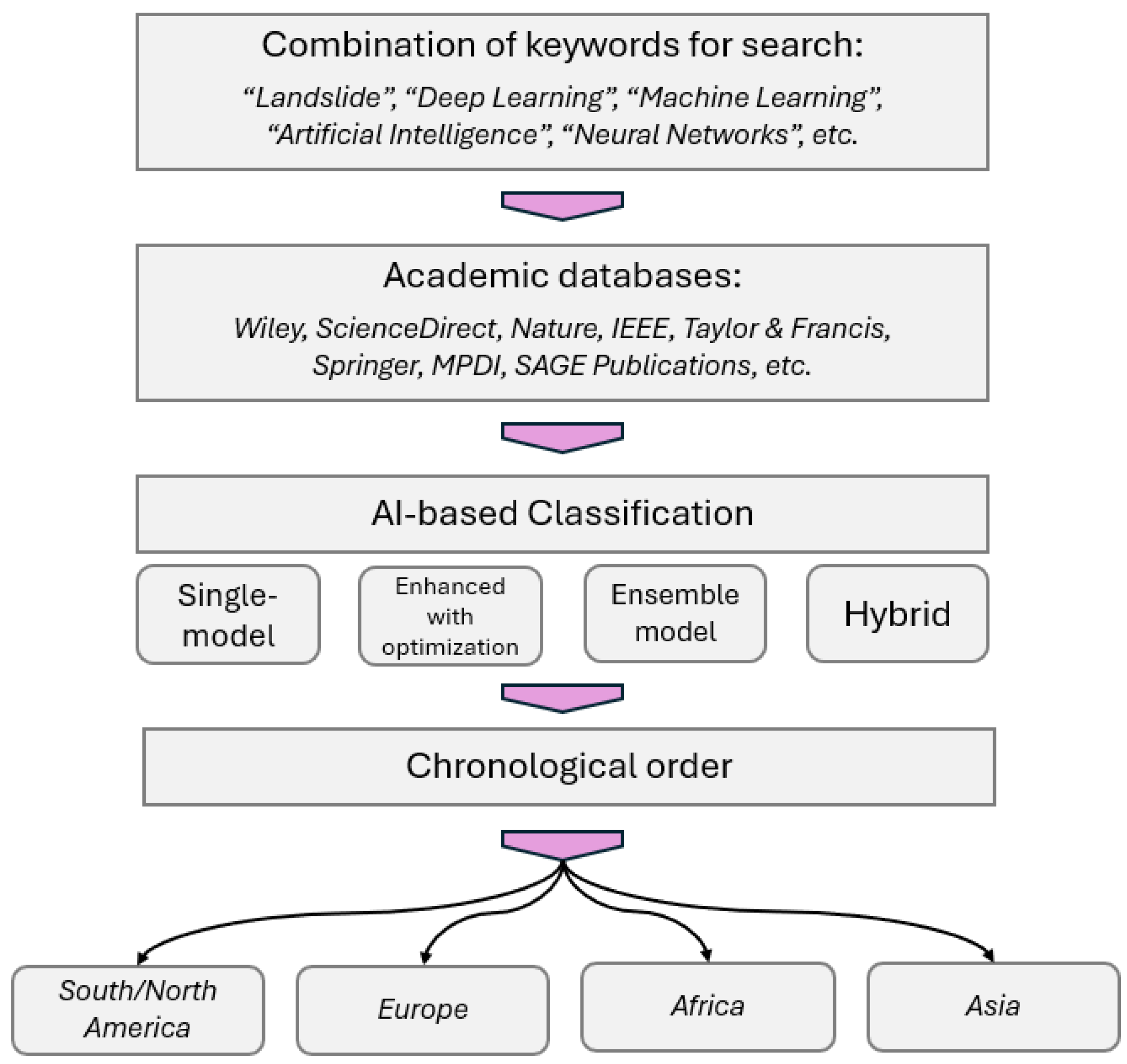
In this review, we conducted a comprehensive literature analysis on the application of AI in LSM focusing on studies published from 2020 onward. The primary goal is to provide insights into recent progress, compare AI methodologies, and identify trends within the field. To gather relevant publications that study landslides using AI-related methods, authors used the world’s leading science databases such as ScienceDirect, Nature, IEEE Xplore, SpringerLink, Wiley Online Library, Taylor & Francis, SAGE Publications, and Google Scholar. The search terms and expressions included combinations of keywords such as “landslide”, “artificial intelligence”, “machine learning”, “deep learning”, “neural networks”, “ensemble learning”, and “geo-spatial analysis” as shown in Figure 1. Thus, the collected works are first classified based on AI methods applied in the studies. For each AI-based classification area, the works are organized chronologically and further divided by region to evaluate which landslide locations are predominantly mapped using AI methods.
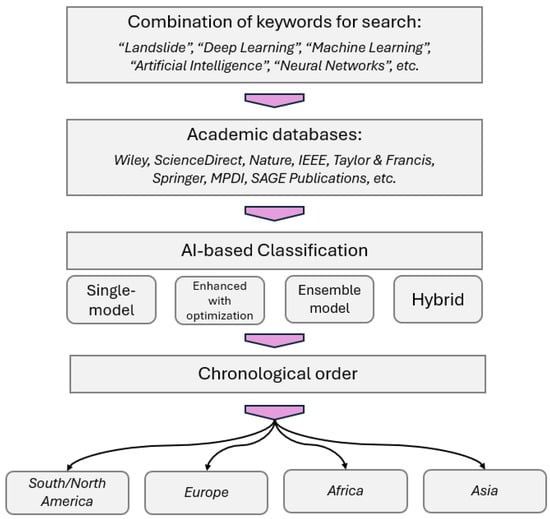
Figure 1.
Workflow of Systematic Literature Review for AI-Based LSM studies.
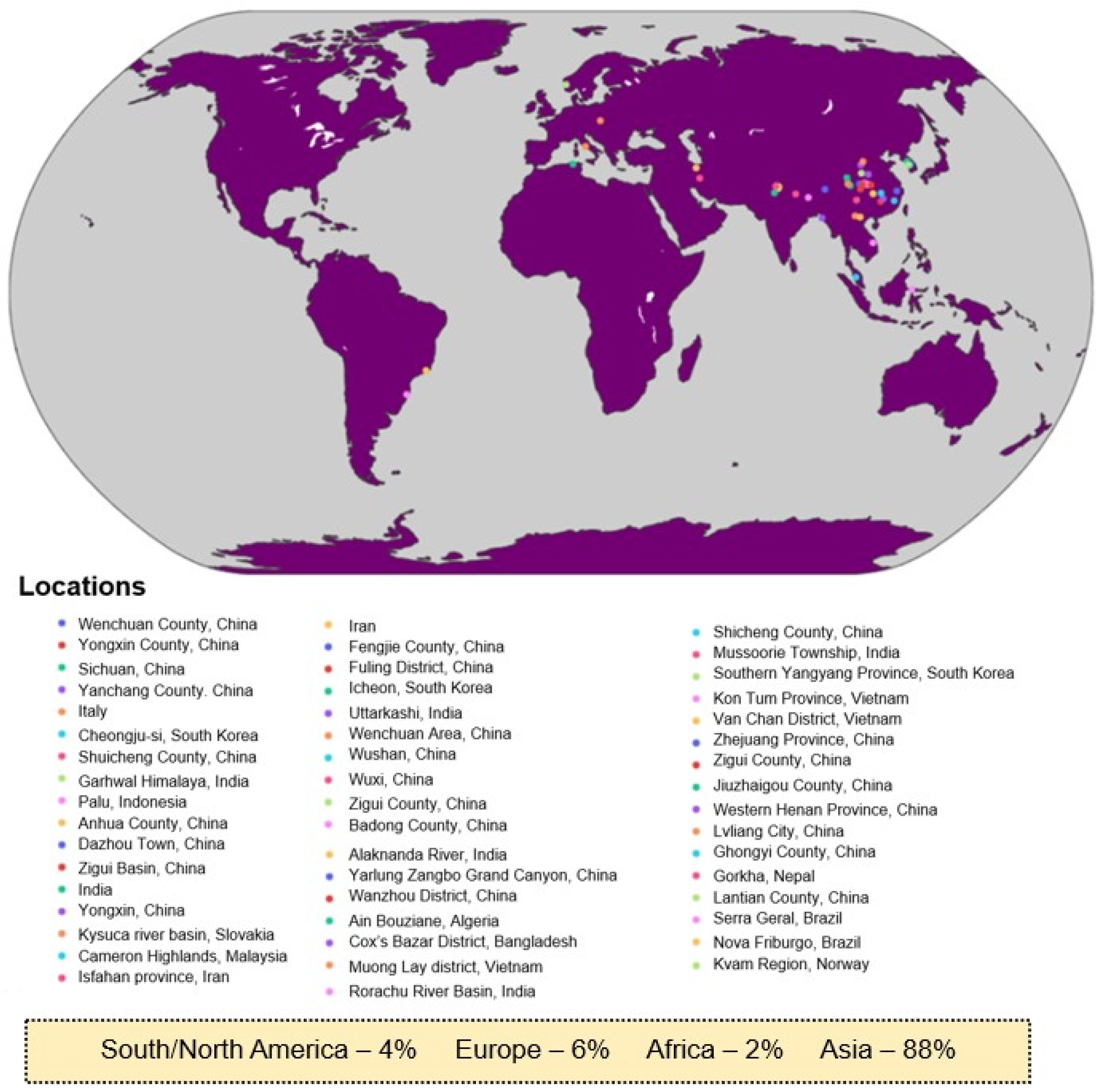
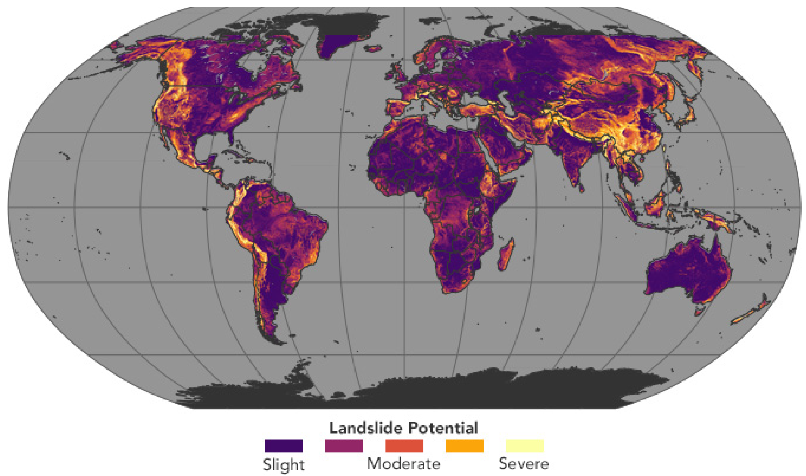
Thus, based on the above-explained workflow, we identified 45 AI-based LSM studies that met the criteria, with the majority (40) of them focused on Asia, 3 based in Europe, and 2 from South and North America (Figure 2). This geographic distribution also reflects global landslide susceptibility trends, as shown in Figure 3, where countries in Asia face heightened landslide risks, driving the adaptation of AI-based LSM research works.
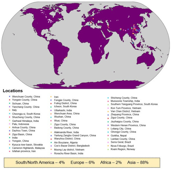
Figure 2.
Geographical locations of the reviewed works on AI-based LSM.

Figure 3.
Global view of landslide susceptibility map (from NASA’s earth observatory database) [14].
For each selected research work, we extracted the following information: AI techniques used, dataset characteristics, conditioning factors, and model performance metrics, including geological, weather information, and software used to train and run AI algorithms. Model performance metrics, such as area under the curve (AUC) and accuracy, are tabulated to facilitate comparison, along with conditioning factors (e.g., slope, normalized difference vegetation index (NDVI), rainfall, etc.) to observe commonalities and differences across studies. We also recorded dataset sizes, sources, and split ratios (e.g., training vs. testing).
The analysis was conducted in three stages. First, a descriptive overview of the selected studies highlighted the prevalence of different AI models, dataset characteristics, and geographic regions. This stage established a baseline understanding of current practices. In the second stage, a comparative analysis evaluated model performance metrics across studies, identifying high-performing models and noting trends in conditioning factor usage based on regional or dataset characteristics. Finally, the studies were classified based their complexity, such as single model, enhanced with optimization, ensemble, and hybrid models to evaluate trends in AI models and performance as well as their strengths, limitations, and applicability in different LSM contexts.
While this review aims to provide a comprehensive analysis of recent AI applications in LSM, certain limitations must be acknowledged. The review is limited to studies published from 2020 onward, potentially excluding valuable insights from earlier research. Additionally, the lack of standardized performance metrics across studies creates challenges for direct comparisons of model efficacy. Nonetheless, this methodology ensures a systematic, comprehensive, and comparative approach to understand recent advances in AI-based LSM and provides useful guidance for future research in this area.
3. Overview of Al Techniques in LSM
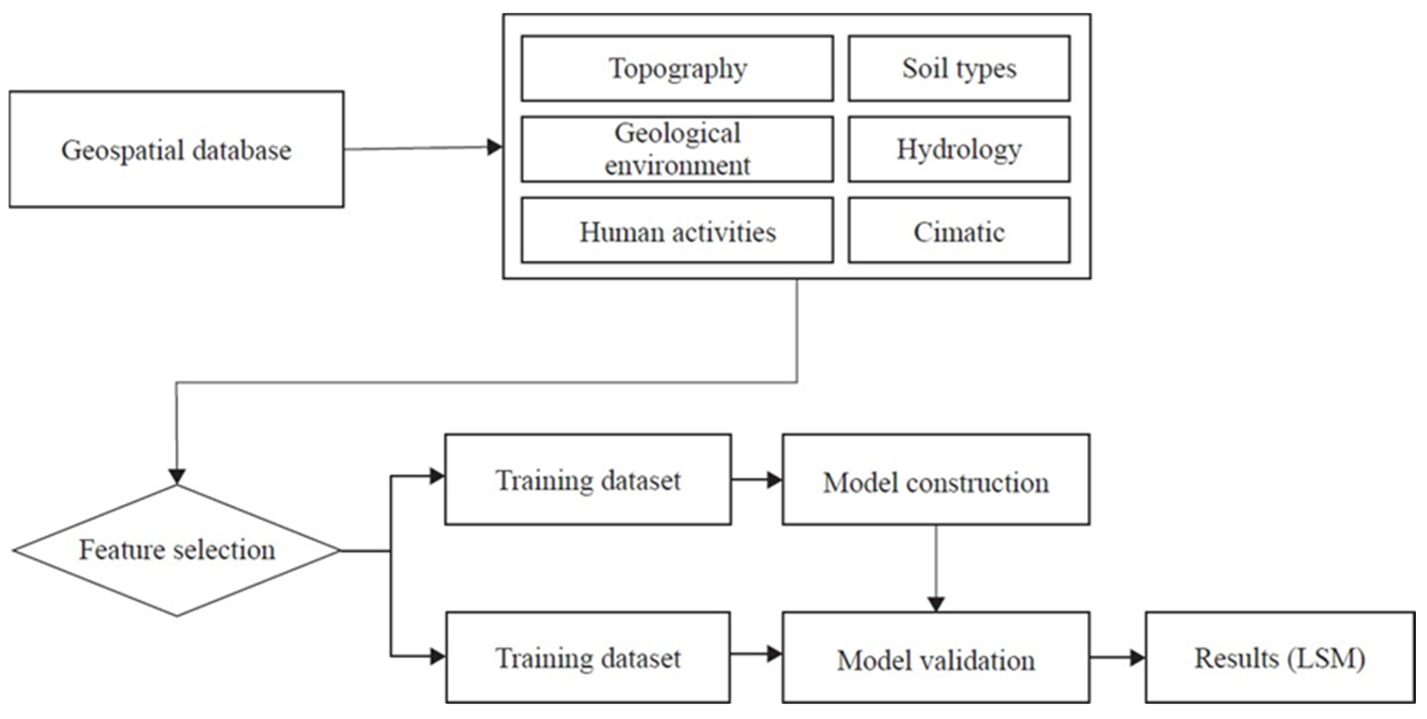
The overall steps of AI-based LSM development consist of mainly data collection, data processing, selection of AI models, training, validation, and creation of the optimized deployable method to predict LSM as shown in Figure 4. Data collection is typically carried out by using GIS software, site surveys, and historical records of landslides, and the collected data are further processed and optimized to be used in the AI models. Based on the current review, most works utilize a training-to-validation ratio of 70% to 30% for their models.
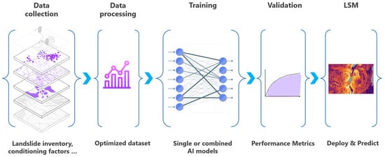
Figure 4.
Flowchart of AI models used to develop LSM.
Based on this review, AI models for LSM can be broadly categorized into single models, enhanced with optimization, ensemble models, and hybrid models. Single models include conventional ML and DL algorithms applied individually, while optimized and combined models involve two or more models working in tandem to improve predictive accuracy. Each classification represents a different level of methodological complexity and adaptability, offering insights into how AI techniques address specific challenges in LSM, from handling data scarcity to capturing intricate spatial patterns.
The accuracy of the AI models designed to assess landslide susceptibility depends mainly on conditioning factors, dataset size, and selected AI techniques. Using Sankey diagram, firstly we visualized which conditioning factors are mostly used in AI models, and further linked them with AI models. The results are given in Figure A1 (see Appendix A). Thus, in the first column, factors influencing landslides are listed, and thickness of each factor shows how frequently they are used in AI models. As can clearly be noticed, slope, aspect, elevation, lithology, plan curvature, profile curvature, average annual rainfall, NDVI, distance to rivers, distance to faults, topological witness index (WTI), land use, and sediment transport index (STI) are the ones mostly used.
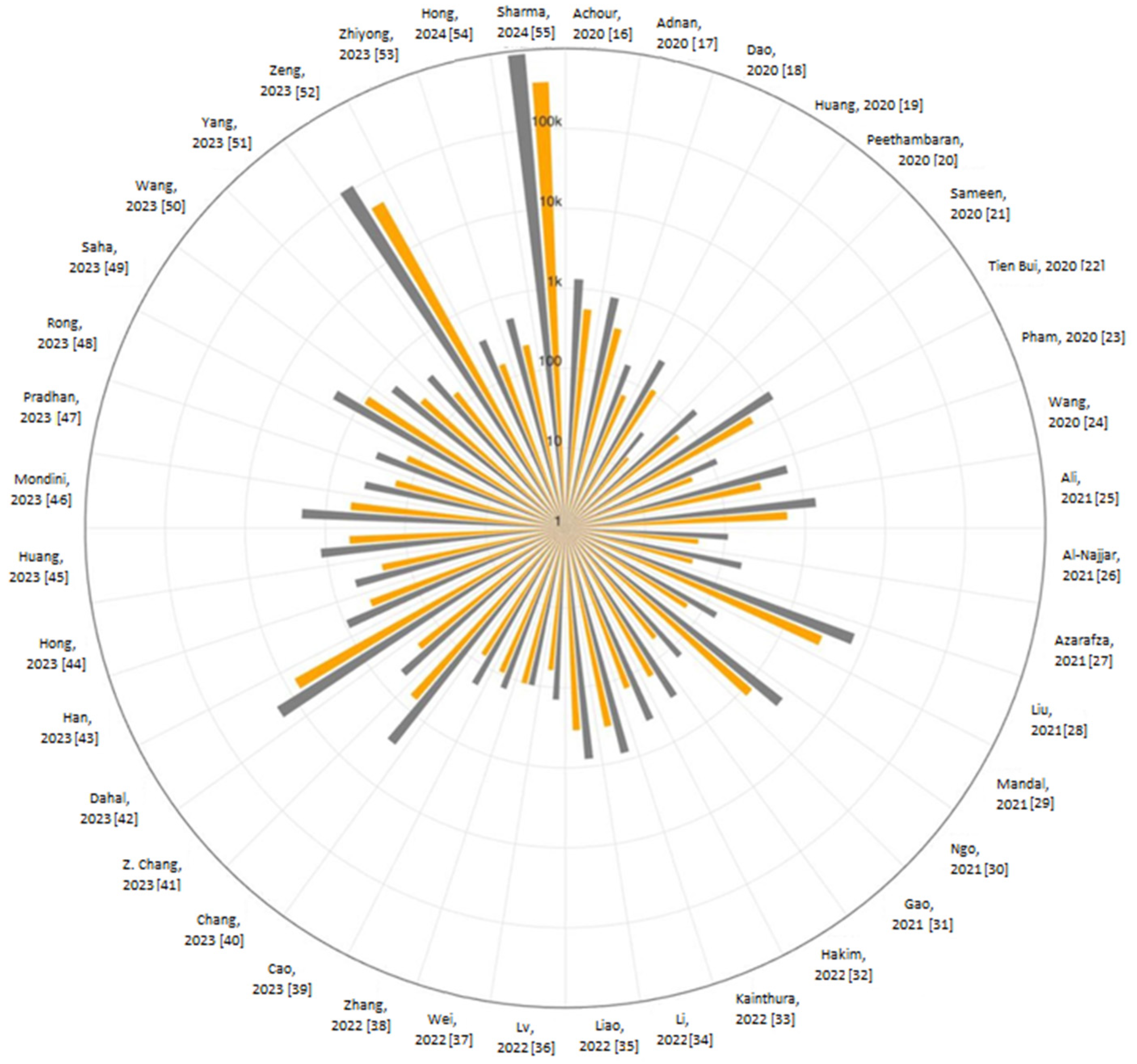
Across the reviewed literature, this study identifies 122 conditioning factors, reflecting a significant increase compared to earlier reviews. For example, Pourghasemi et al. [15], who reviewed studies published from 2005 to 2016, reported a total of 95 conditioning factors. This expanded list highlights recent advances in remote sensing, GIS technologies, and computational power, which enable the use of a broader range of factors for improved model accuracy and adaptability. In addition, Figure 5 shows the recent AI-based LSM works and their associated dataset sizes, which range significantly depending on the model requirements and availability of regional data.
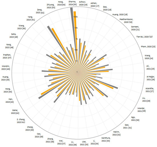
Figure 5.
The latest AI-based LSM works and related dataset sizes [16,17,18,19,20,21,22,23,24,25,26,27,28,29,30,31,32,33,34,35,36,37,38,39,40,41,42,43,44,45,46,47,48,49,50,51,52,53,54,55].
The choice of AI technique is another crucial component in LSM. According to the reviewed studies ML algorithms such as random forest (RF), support vector machine (SVM), and DL models like convolutional neural networks (CNN), multilayer perception (MLP) are the most frequently used. These models are often adopted as baseline models due to their widespread application and proven efficacy in various geographic settings. Each model offers unique advantages: RF is valued for its robustness in handling large datasets and multiple conditioning factors, SVM is known for its high precision in binary classification, CNNs excel in spatial data processing through layered feature extraction, and MLP networks provide flexibility in capturing complex, non-linear relationships between factors.
In recent years, advances in deep learning have introduced different models leveraging multi-layered architectures to enhance predictive capabilities. Deep learning models are particularly useful for handling large, heterogeneous datasets and have shown potential in identifying complex spatial patterns in landslide-prone areas. However, deep learning models typically require larger datasets and greater computational power compared to traditional machine learning models, which may limit their application in regions with limited data availability.
Furthermore, ensemble methods have become increasingly popular as researchers seek to improve prediction accuracy by combining multiple AI models. For example, hybrid models that integrate RF and SVM or CNNs with other neural network architectures are emerging as effective approaches in LSM. The combined approach allows these models to address specific limitations of individual algorithms and leverage their combined strengths. Ensemble models have shown promise in improving model stability and reducing the effects of overfitting, making them valuable tools for LSM in diverse environments.
Overall, the integration of AI in LSM has evolved from the use of single machine learning models to more complex and adaptive methods, including optimization, ensemble learning and hybrid approaches. This progression reflects ongoing improvements in computational resources and the expanding availability of high-resolution geospatial data, which continue to drive innovation in landslide susceptibility assessment. As the field advances, the role of AI in LSM is expected to grow, with hybrid models and explainable AI techniques offering promising avenues for future research.
4. Complexity-Based Classification of AI Models in LSM
This section provides a comprehensive classification of AI models applied to LSM based on their complexity, with models grouped into four main categories: single-model approaches, enhanced models with optimization, ensemble models, and hybrid models. Each classification represents a different level of methodological complexity and adaptability, offering insights into how AI techniques address specific challenges in LSM, from handling data scarcity to capturing intricate spatial patterns.
- Single-model approaches focus on individual ML or DL models without additional modifications, providing a baseline for landslide prediction and highlighting the potential of each model in isolation. This category illustrates the strengths and limitations of popular algorithms such as RF, SVM, and CNN when used independently in LSM;
- Enhanced models with optimization introduces advanced optimization techniques to improve the performance of single models, particularly in challenging terrains or data-limited environments. Techniques like Bayesian optimization, class weighting, and transfer learning are utilized to tackle issues such as sample imbalance, hyperparameter tuning, and data scarcity, yielding more accurate and adaptable LSM models;
- Ensemble models combine multiple base models to improve predictive accuracy and robustness across diverse terrains. Techniques such as stacking, bagging, and blending enhance model performance by aggregating strengths from different algorithms, with separate strategies for ML and DL ensembles to address specific environmental complexities in LSM;
- Hybrid models integrate multiple AI techniques within a single framework, combining ML and DL methods or blending optimization and ensemble techniques. These models are particularly suited for high-dimensional or complex terrains, where capturing interactions between diverse conditioning factors is critical for accurate LSM.
This classification provides a structured approach to understanding how AI models have been adapted and improved for LSM. Each category offers distinct advantages and is suited to specific geographic and data conditions, enabling the selection of an optimal model type based on the complexity and requirements of the mapping task.
The main findings are tabulated and provided as Table A1 (see Appendix A). In the table, the geographic location from where the dataset is developed, type of AI models used, dataset size, and the performance of the models can be found. Moreover, for each study selected, conditioning factors are listed, and main information such as slope range, annual precipitation, and mean temperature of the locations are also provided in Table A1.
4.1. Single-Model Approaches
Single-model approaches offer an essential foundation in LSM by applying individual models to assess landslide-prone regions. This structured review examines 17 studies, highlighting the strengths, limitations, and practical applications of ML and DL models across various terrains. Although most of the works used several AI models in their studies, we tried to divide the discussion into ML and DL models, to enable a clearer understanding of model performance in different environments.
4.1.1. Traditional ML Models
Traditional ML models have demonstrated solid performance in LSM, especially in linear, structured, or moderately complex terrains where relationships between conditioning factors are relatively straightforward. Techniques like RF, SVM, and decision trees (DT) are widely valued for their computational efficiency and interpretability, which make them particularly effective in infrastructure-heavy or linear regions with defined environmental features.
For example, RF, SVM, and boosted regression tree (BRT) were applied along Algeria’s A1 highway, a structured and linear environment [16]. RF emerged as the top performer with an AUC of 0.972, showing its robustness in capturing direct relationships among factors like slope and lithology. The structured nature of the highway corridor proved ideal for RF, as its algorithmic design captures clear, well-defined patterns effectively. Compared to SVM and BRT, RF’s superior AUC underscores its advantage in infrastructure-focused LSM applications, where interpretability and computational efficiency are crucial.
Huang et al. [19] conducted a broader study in China, comparing eight models, including analytic hierarchy process (AHP), binary logistic regression (BLR), MLP, and C5.0 DT. Here, C5.0 DT achieved the highest AUC of 0.868, highlighting its effectiveness in handling non-linear relationships. However, the slightly lower AUC relative to RF in Algeria suggests that decision trees may perform best in environments where relationships among factors are somewhat linear but can handle moderate variability. This study reveals ML’s limitations in highly variable terrains, where models like C5.0 DT may be less effective without ensemble or boosting methods.
Liu et al. [28] evaluated RF and gradient boosted regression tree (GBRT) in Norway’s varied Kvam region, achieving AUC values of 0.85 and 0.87, respectively. The slight edge of GBRT over RF indicates that gradient-boosting techniques may have an advantage in capturing complex susceptibility patterns in moderately variable terrains. In contrast, RF’s higher AUC of 0.972 in Algeria’s more linear terrain reinforces that ML models like RF are well-suited to environments with defined, consistent features, while GBRT is more adaptable to moderate variability.
Finally, in another work, Huang et al. [56] studied the impact of spatial resolution and conditioning factors on LSM accuracy (Figure 6) in Yanchang County, China, with RF achieving the highest AUC (>0.90) at 15 m resolution. This finding suggests that ML models like RF perform best with high-resolution data, where detailed variations can be captured accurately. The study reinforces RF’s suitability for data-rich environments and illustrates that ML models are ideal for settings where high spatial resolution is feasible, offering both precision and computational efficiency.
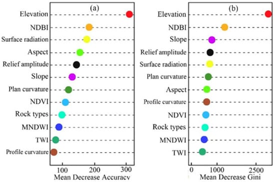
Figure 6.
The importance of conditioning factors in the accuracy of LSM development by Huang et al. [56].
In summary, ML models exhibit strong performance in structured, moderately complex terrains and regions with high-resolution data. RF and GBRT consistently achieve high AUC values in linear or infrastructure-focused environments, where interpretability and efficiency are priorities. However, ML models may be limited to highly variable landscapes, as they typically require careful tuning to adapt to complex interactions among environmental factors.
4.1.2. DL Models
DL models bring distinct advantages to LSM, especially in complex, heterogeneous terrains and high-stakes, data-intensive regions. Techniques like CNN, recurrent neural network (RNN), and DenseNet consistently outperform traditional ML models in capturing intricate spatial and temporal patterns, making them ideal for environments with highly variable or expansive landscapes.
In the diverse terrain of Vietnam’s Muong Lay district, Dao et al. [18] applied spatially explicit DL neural network, achieving an AUC of 0.90. The model’s ability to capture non-linear and diverse interactions among factors made it well-suited for this complex landscape. DL’s adaptability to highly variable geo-environmental features illustrate its suitability for heterogeneous areas, where traditional ML models may struggle with non-linear patterns and diverse inputs.
Mandal et al. [29] used CNN in the Sikkim Himalayas, achieving higher performance than RF and ANN in this rugged, landslide-prone region. CNN’s architecture excels at capturing spatial dependencies, which is essential in mountainous terrains where topographic variability drives susceptibility. Compared to RF’s strong performance in linear regions, CNN’s advantage in the Sikkim Himalayas underscores DL’s effectiveness in handling high variability and complex terrain interactions.
In Iran, Ngo et al. [30] applied RNN and CNN, achieving AUCs of 0.88 and 0.85, respectively. The slightly higher AUC for RNN highlights its utility in environments with temporal variability, making it particularly suitable for regions where factors like rainfall or seismic activity fluctuate over time. RNN’s temporal sensitivity gives it an edge over CNN in dynamic environments, while CNN remains effective in capturing spatially stable susceptibility factors.
FC-DenseNet was applied in China’s Zigui and Jiuzhaigou counties (Figure 7), achieving kappa values above 94% and outperforming U-Net and ResU-Net [31]. The model’s boundary-detection capabilities make it ideal for areas with overlapping environmental triggers, where precise delineation is essential. This demonstrates DL’s strength in complex, high-risk environments where multiple factors intersect, showcasing its ability to manage multifactorial data better than ML models.
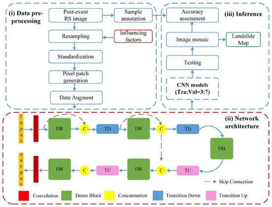
Figure 7.
Application of FC-DenseNet for LSM by Gao et al. [31].
In large-scale areas, such as Brazil’s Serra Geral, Gameiro et al. [57] applied an artificial neural network (ANN), achieving an AUC of 0.954, while Soares et al. [58] used CNN across varied Brazilian landscapes. The adaptability of ANN and CNN in expansive, heterogeneous terrains underscores DL’s advantage in large-scale LSM applications, where capturing broad susceptibility patterns is crucial. Compared to ML’s utility in more contained regions, DL’s scalability and precision make it a strong choice for extensive, diverse geographies.
Bui et al. [22] implemented a Deep Learning Neural Network (DLNN) model to predict landslide occurrences in Kon Tum Province, Vietnam, utilizing nine conditioning factors, including slope angle, elevation, aspect, land use, NDVI, soil type, and distances to faults and geological boundaries. The study compiled a dataset of 1657 recorded landslide events from 2004 to 2015, categorizing landslides by size to capture variability in susceptibility. The data were split into 70% for training and 30% for validation, ensuring a balanced distribution of landslide and non-landslide instances. To evaluate the DLNN model’s performance, comparisons were made with other single-model approaches, including SVM, C4.5 decision trees, MLP neural networks, and Random Forest (RF). This comparative analysis highlights the effectiveness of DLNNs as standalone models in LSM, with findings suggesting that DLNNs can provide robust predictive accuracy when contrasted with other traditional ML algorithms.
Azarafza [27] employed a deep convolutional neural network (CNN–DNN) model for LSM in Iran’s Isfahan province, marking one of the first applications of this model at such a scale in the region. Developed using historical landslide records, remote sensing images, and various environmental factors, the CNN–DNN model demonstrated superior predictive accuracy, outperforming benchmark models such as SVM, Logistic Regression (LR), Gaussian Naive Bayes (GNB), Multi-Layer Perceptron (MLP), Bernoulli Naive Bayes (BNB), and Decision Tree (DT) classifiers. Achieving an AUC of 90.9% and lower error indices (MSE = 0.17, RMSE = 0.40, MAPE = 0.42), the CNN–DNN model effectively handled the spatial complexities of landslide prediction, highlighting its advantages over conventional pixel-based methods. This study reinforces the capability of advanced CNN–DNN architectures in capturing intricate spatial relationships for improved LSM accuracy.
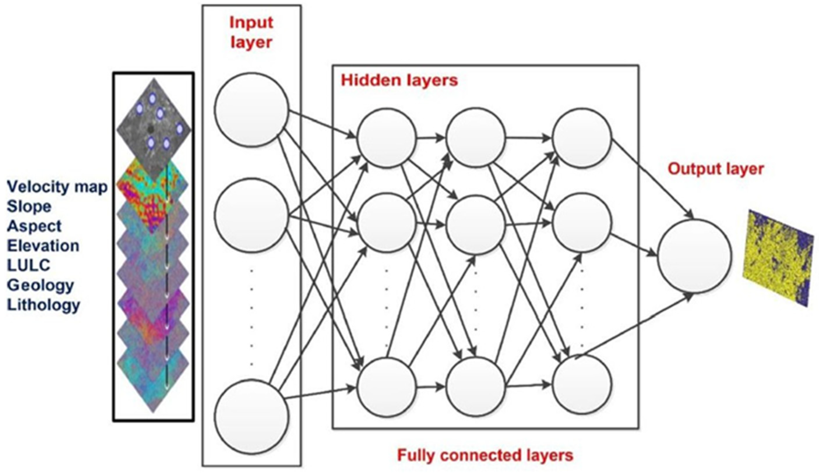
In India’s high-risk Srinagar-Rudraprayag region, Meghanadh et al. [59] developed a deep multilayer perceptron for LSM (DMLP-LSM) (Figure 8), integrating multi-temporal interferometric synthetic aperture radar data to achieve an AUC of 0.907 with high precision (92.11%) and specificity (95.55%). The radar-enhanced DL model demonstrates DL’s potential in real-time, data-intensive applications. Compared to RF’s performance in less dynamic environments, DMLP-LSM’s ability to integrate complex datasets illustrates DL’s utility in high-stakes regions where rapid, accurate assessments are critical.

Figure 8.
Schematic view of DMLP-LSM [59].
Finally, Pradhan et al. [47] used CNN in South Korea, achieving an accuracy of 89% with SHAP-based interpretability. This integration of SHAP values highlights DL’s capability to deliver transparent, actionable insights for landslide risk, especially in regions where clear, interpretable predictions are needed.
In summary, DL models achieve high accuracy and flexibility in heterogeneous and data-rich terrains. Techniques like CNN, RNN, and DenseNet consistently outperform ML models by capturing intricate, non-linear interactions, making them suitable for complex landscapes with variable conditions. However, DL models are computationally demanding and may require large datasets, which can limit their use in resource-constrained environments. In expansive, dynamic, or multifactorial settings, DL’s adaptability and high-dimensional modeling capabilities offer unparalleled precision, supporting LSM applications where high accuracy and scalability are essential.
4.2. Enhanced Models with Optimization
Enhanced models with optimization mark a significant advancement in LSM, where optimization techniques are applied to traditional ML and DL models to improve predictive accuracy, especially in complex or data-limited environments. By integrating methods like Bayesian optimization, class weighting, and metaheuristic algorithms, these models effectively handle challenges such as sample imbalance, hyperparameter tuning, and data scarcity. This section reviews optimization approaches applied to both ML and DL models, detailing how each enhancement strategy contributes to more reliable LSM predictions and greater model adaptability across varied terrains.
4.2.1. Traditional ML Models with Optimization
Optimization techniques significantly improve ML models in LSM by addressing common issues such as sample imbalance, class weighting, and data scarcity. These methods refine model inputs and training processes, allowing ML models to capture complex patterns in landslide-prone areas with greater accuracy.
Cao et al. [39] demonstrated that feature selection can enhance ML model accuracy. Using recursive feature elimination (RFE) with XGBoost as shown in Figure 9, they achieved an AUC of 0.89, underscoring how focusing on influential factors can improve performance without adding computational complexity. Compared to general applications of RF, this tailored approach highlights XGBoost’s adaptability in moderately complex landscapes, especially when a focused feature selection can streamline input data effectively.
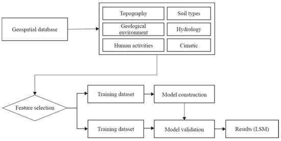
Figure 9.
Schematic illustration of ML-based LSM from the research work [39].
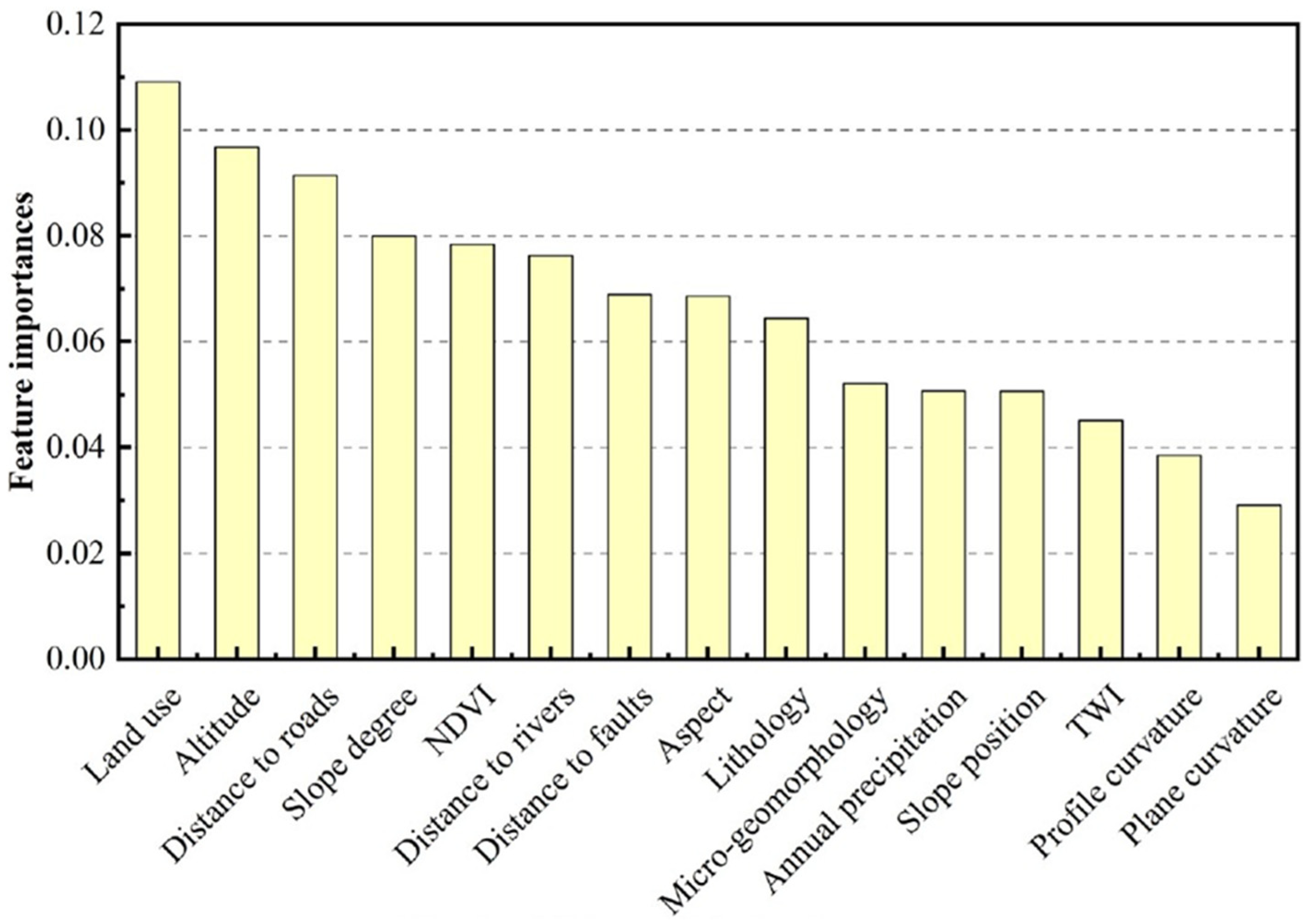
Yang et al. [51] in Anhua County, China, employed Bayesian optimization to optimize the ratio of positive to negative samples in ML models for LSM. By adjusting the balance between landslide and non-landslide samples, they addressed a key issue of dataset imbalance, which often reduces predictive accuracy. With optimized sample ratios, RF achieved the highest AUC of 0.840, outperforming GBDT at 0.831 and SVM at 0.775. This study demonstrates Bayesian optimization’s effectiveness in fine-tuning sample distributions to achieve more accurate predictions, particularly in varied terrains. In contrast to standard approaches, this technique not only increased predictive power but also maintained model robustness across different landscape features. In addition to optimizing the sample ratio, the study examined the selection of key conditioning factors for LSM models. Fifteen factors were included in the analysis, such as altitude, slope degree, lithology, land use, and distance to faults, which were selected based on the characteristics of the study area and data availability, which can be seen in Figure 10.

Figure 10.
Importance evaluation of landslide conditioning factors by Yang et al. [51].
Zhang et al. [38] tackled class imbalance in China’s Three Gorges Reservoir area using a class-weighted algorithm with logistic regression (LR) and ensemble models such as LightGBM and RF. By assigning different misclassification penalties to landslide and non-landslide samples, they transformed LSM into a cost-sensitive task. The weighted RF model achieved the best performance in terms of AUC, balanced accuracy, and geometric mean scores, outperforming unweighted models. Compared to Yang et al.’s [51] sample balancing approach, this study highlights class weighting as an effective optimization strategy for regions where landslides are underrepresented in datasets. The findings emphasize the adaptability of cost-sensitive algorithms in environments with imbalanced data, where class-specific weighting aligns predictions with real-world landslide distributions.
In data-scarce regions, Zhiyong [53] applied TrAdaBoost, a transfer learning algorithm, to enhance LSM in the Zigui Basin and Wenchuan-Yingxiu region by transferring knowledge from one landslide inventory to another. Leveraging historical landslide data from a similar region, TrAdaBoost minimized the need for new data collection and achieved an AUC of 0.85, outperforming conventional ML models like DT at 0.73, SVM at 0.82, and RF at 0.83. This approach illustrates the power of transfer learning in generating reliable LSM predictions for data-limited terrains, addressing a significant limitation in ML models that rely on extensive datasets. The comparison with Yang et al.’s Bayesian optimization underscores TrAdaBoost’s utility in environments where data scarcity is a constraint, offering a cost-effective alternative to traditional ML approaches.
Collectively, these studies showcase how sample balancing, class weighting, and transfer learning optimize ML models for LSM. By addressing limitations like sensitivity to data imbalance and reliance on extensive datasets, these optimization techniques make ML models more adaptable for diverse terrains and data conditions, enhancing accuracy and computational efficiency.
4.2.2. DL Models with Optimization
In recent years, DL models in LSM have also benefited from advanced optimization techniques, such as Bayesian optimization and metaheuristic algorithms, which fine-tune complex architectures and address issues like overfitting and parameter selection. These methods are particularly valuable in data-constrained or highly variable terrains where precise tuning is essential for reliable predictions.
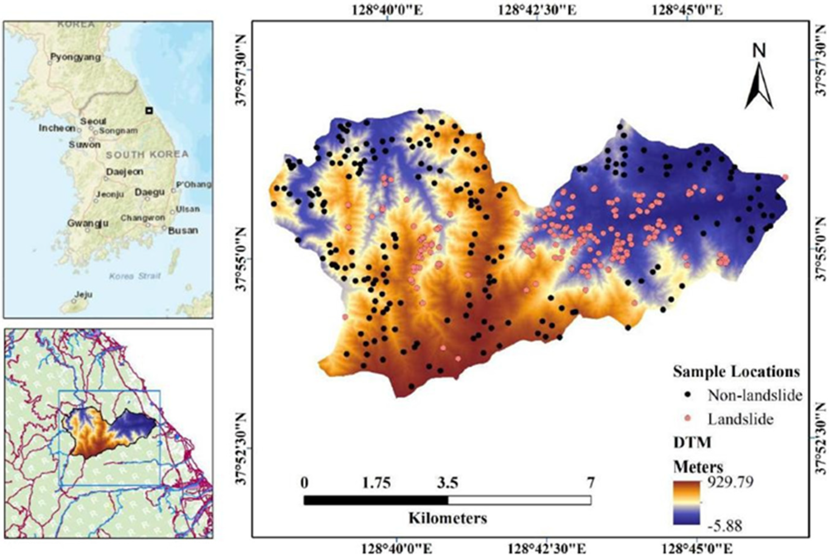
Sameen et al. [21] employed Bayesian optimization on a 1D-CNN in South Korea’s Yangyang Province as shown in Figure 11, to improve model performance on a small dataset. Through Bayesian hyperparameter optimization, they increased the AUROC of the CNN model to 0.880 on the test set and 0.893 on cross-validation, outperforming traditional models like ANN and SVM. The optimization process enhanced the CNN’s accuracy by approximately 3%, addressing potential overfitting through precise dropout rates and feature selection. This study highlights the role of Bayesian optimization in refining DL models for complex terrains with limited data, enhancing their predictive reliability without excessive computational burden.

Figure 11.
Landslide inventory map of the area: Southern Yangyang Province, South Korea [21].
Dahal and Lombardo [42] applied an explainable artificial intelligence (XAI) approach to enhance an ANN model for LSM in the Gorkha earthquake-affected region of Nepal. They utilized the dataset from Roback et al. [60], which recorded 24,903 coseismic landslides. Using SHapley Additive exPlanations (SHAP), they improved the interpretability of the model’s predictions, which were based on 13 conditioning factors. Structured with 12 hidden layers, the ANN model achieved a high AUC of 0.89, outperforming traditional models like SVM and RF. This enhanced approach illustrates the value of adding interpretability to complex models, particularly in high-risk regions, where understanding the influence of conditioning factors is as important as prediction accuracy.
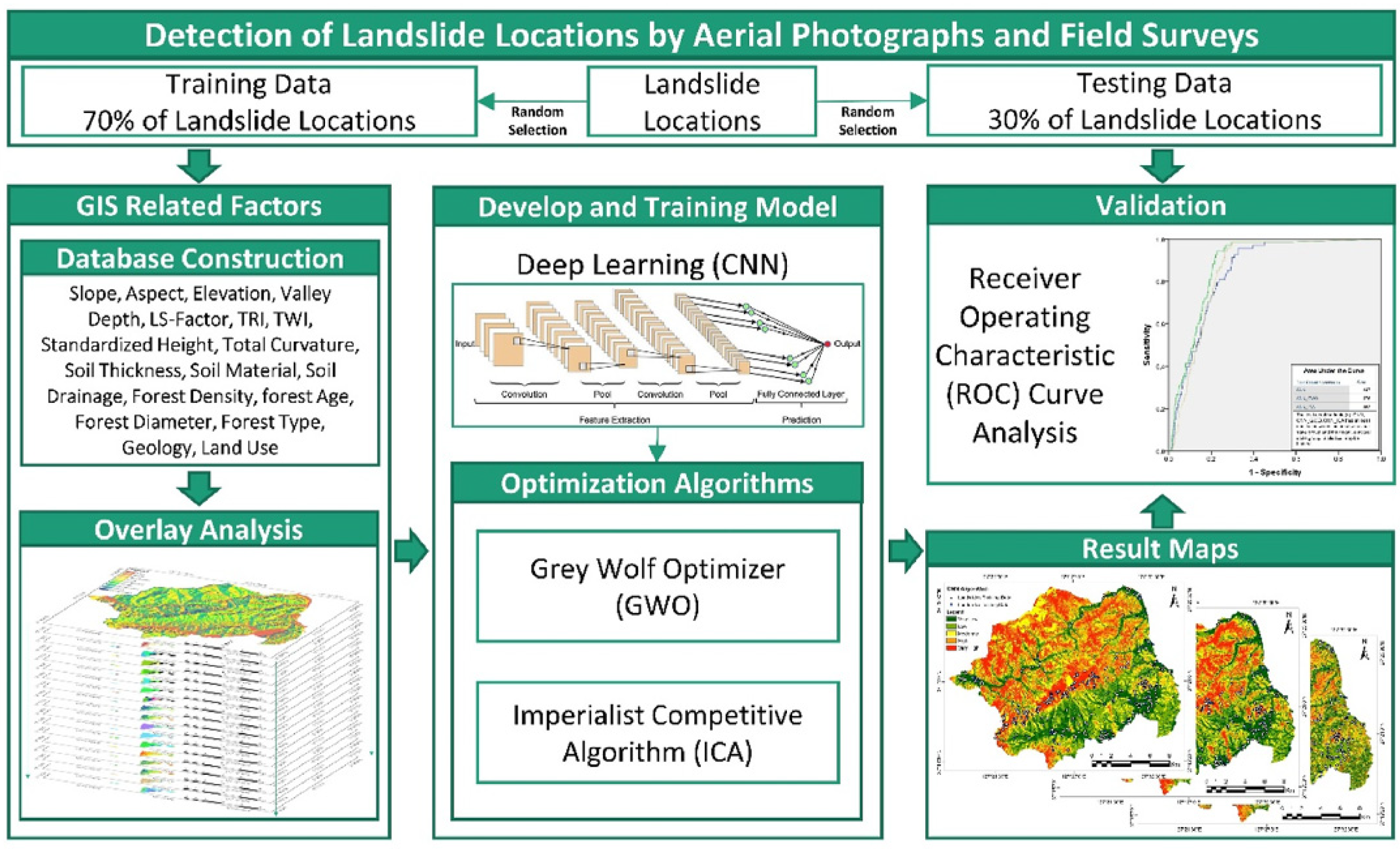
Hakim et al. [32] integrated metaheuristic optimization methods—specifically the grey wolf optimizer (GWO) and the imperialist competitive algorithm (ICA)—with CNNs in Icheon City, South Korea, as shown in Figure 12. By optimizing CNN parameters using GWO and ICA, they achieved improved AUC values of 0.876 and 0.852, respectively, surpassing the standalone CNN’s AUC of 0.847. The CNN-GWO model not only achieved a 2.9% improvement in ROC but also reduced mean square error (MSE) and root mean squared error (RMSE), indicating better alignment between model predictions and observed data. Compared to Bayesian optimization in Sameen et al. [21], the metaheuristic approach here demonstrates the advantages of GWO and ICA in complex, topographically diverse landscapes where conventional parameter tuning may fall short.

Figure 12.
Methodology of the study by Hakim et al. [32].
Each of these studies underscores how advanced optimization strategies enable DL models to adapt to complex and data-constrained environments. Through fine-tuning of hyperparameters and integration of metaheuristic methods, DL models achieve higher accuracy and resilience against overfitting, critical for LSM in highly variable regions where DL architectures need flexibility to capture nuanced patterns.
Optimization techniques elevate the performance and adaptability of both ML and DL models in LSM. ML models become more versatile in structured, data-limited environments, while DL models achieve the precision needed for complex, variable terrains. Together, these enhanced models with optimization represent a substantial advancement in landslide susceptibility mapping, enabling more reliable, context-specific predictions across diverse geographic conditions.
4.3. Ensemble Models
Ensemble models are increasingly utilized in LSM to improve predictive accuracy by combining multiple base models. These methods aggregate the strengths of diverse algorithms, capturing complex spatial patterns and enhancing model robustness across varied terrains. This section reviews studies on ML and DL ensemble models, highlighting the distinct benefits of each approach in specific landscapes and data conditions.
4.3.1. Traditional ML Ensemble Models
ML ensemble models in LSM enhance accuracy and resilience by combining multiple algorithms through techniques such as stacking, bagging, and blending. These approaches are especially effective for handling data variability and are well-suited for regional and national-scale assessments.
In Cox’s Bazar, Bangladesh, researchers [17] developed an ensemble model using multivariable logistic regression to combine four ML algorithms: K-Nearest Neighbor (KNN), Multi-Layer Perceptron (MLP), RF, and SVM. By integrating these models, the ensemble achieved a high AUC of 0.97, up from 0.93 to 0.96 for the individual models. This improvement highlights the ensemble’s ability to reduce spatial discrepancies, resulting in a more reliable susceptibility map with correlation coefficients between 0.88 and 0.92. This study underscores the capacity of ML ensembles to unify predictions in regions with diverse terrain features, particularly when spatial consistency is critical.
Saha et al. [49] conducted a study on LSM in the Garhwal Himalaya region, an area characterized by complex geological structures and active tectonic activity, resulting in frequent landslide-induced fatalities. They applied a range of ML and DL algorithms, including SVM, RF, bagging, ANN, and DLNN. These models were trained and tested using twenty conditioning factors such as slope, altitude, geology, curvature, aspect, lineament density, and proximity to rivers and roads.
To optimize feature selection, the authors employed multi-collinearity tests and information gain ratio (InGR) statistics, with the most significant factors identified as altitude, drainage density, and distance from roads. The models were trained on a dataset of historical landslide points, split into 70% for training and 30% for testing. Among the models, the DLNN achieved the highest predictive accuracy, with an AUC of 0.925. The study demonstrates the effectiveness of ensemble methods, particularly bagging, in enhancing model reliability for LSM in geologically complex and hazard-prone regions. This approach underlines the value of integrating both ML and DL techniques to address the intricate patterns associated with landslide occurrences.
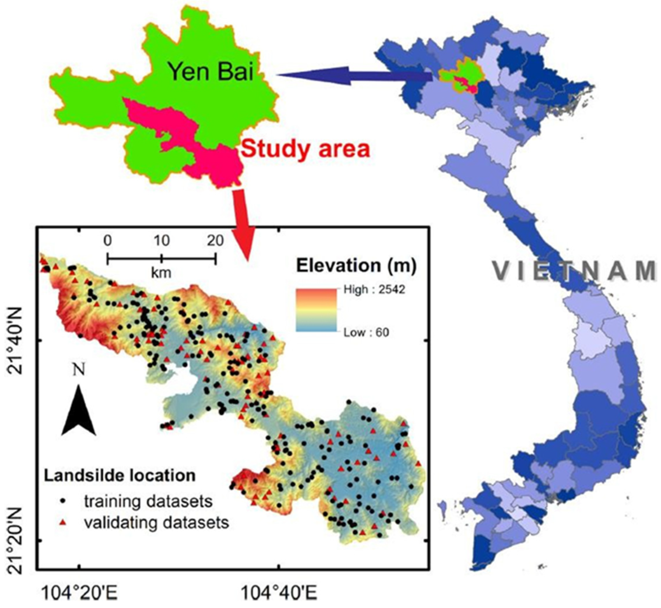
Pham et al. [23] applied radial basis function neural networks (RBFN) with additional ensemble techniques such as Random Subspace (RSS), Attribute Selected Classifier (ASC), Cascade Generalization (CG), and Dagging in Vietnam’s Van Chan district. The study area is illustrated in Figure 13. While the standalone RBFN achieved an AUC of 0.799 in training, the ensemble techniques increased this to an average AUC of 0.83 during validation, demonstrating improved generalizability and performance in mixed terrain. The study showcases ensemble learning’s effectiveness in enhancing predictive accuracy, particularly in areas where individual models struggle with varied topographic characteristics.

Figure 13.
Study area—Van Chan district, Yen Bai Province, Northern Vietnam [23].
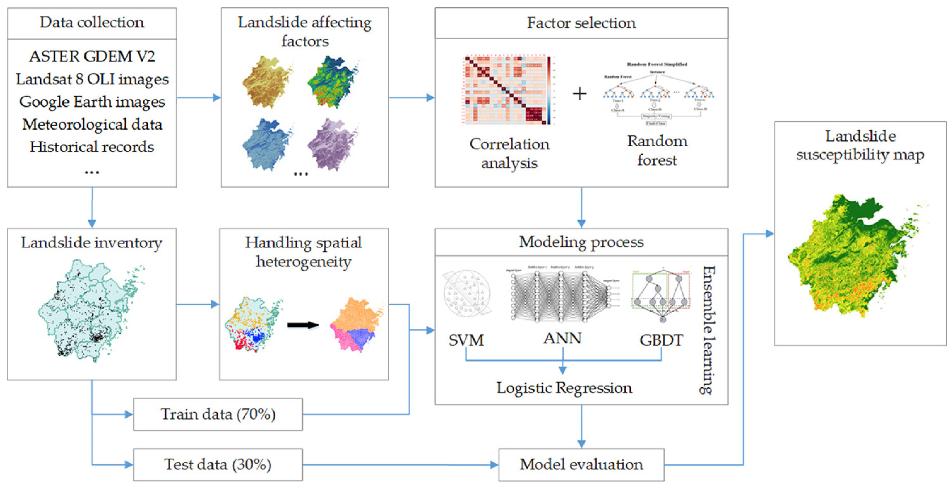
Wang et al. [24] employed a stacking ensemble technique integrating SVM, ANN, and GBDT models in landslide-prone regions, with GeoSOM (a self-organizing mapping modification) applied for further performance enhancement (Figure 14). The GeoSOM-stacking ensemble achieved an AUC of 0.889 and accuracy of 0.812 on testing data, outperforming the individual models and mitigating overfitting issues. The stacking approach was particularly effective here, as it allowed the model to capture complex interactions among conditioning factors, a necessity in variable landscapes prone to landslides.
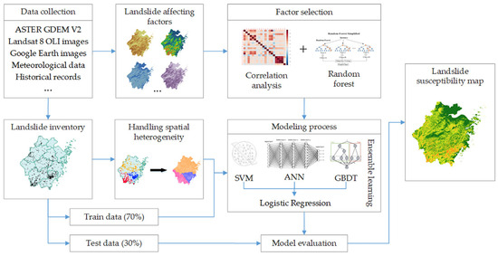
Figure 14.
Diagram of the ML methods for LSM [24].
In a national-scale study in India [55], researchers applied a blending ensemble approach by combining ANN, RF, and SVM, with logistic regression as the meta-model to handle class imbalance through undersampling and oversampling. The blending ensemble outperformed each individual model, demonstrating its effectiveness in capturing broad susceptibility patterns across diverse terrain. This study highlights the applicability of blending for large-scale LSM, where diverse environmental factors require a flexible model capable of generalizing across regions.
Together, these studies illustrate the strengths of traditional ML ensemble models in enhancing LSM accuracy, with stacking, blending, and bagging approaches proving particularly adaptable for diverse terrains. From regional-scale assessments in complex landscapes to national mappings, ML ensemble techniques offer valuable solutions for capturing varied susceptibility patterns, achieving high accuracy and consistency.
4.3.2. DL Ensemble Models
By combining neural networks or applying ensemble strategies to DL architectures, these models capture intricate spatial relationships, providing robust predictions in challenging, data-rich terrains.
Mondini et al. [46] applied an ensemble approach using bagging techniques with Fully Connected Neural Networks (FCNN) to forecast rainfall-induced landslides over large areas. They trained 100 different FCNN models with hourly rainfall data, achieving accuracies between 78.3% and 84.8% across models. The bagging ensemble stabilized performance over longer rainfall lag periods, yielding reliable predictions even in complex rainfall-induced landslide scenarios. This study underscores DL ensembles’ operational utility in dynamic regions, highlighting bagging’s role in improving stability for highly variable inputs.
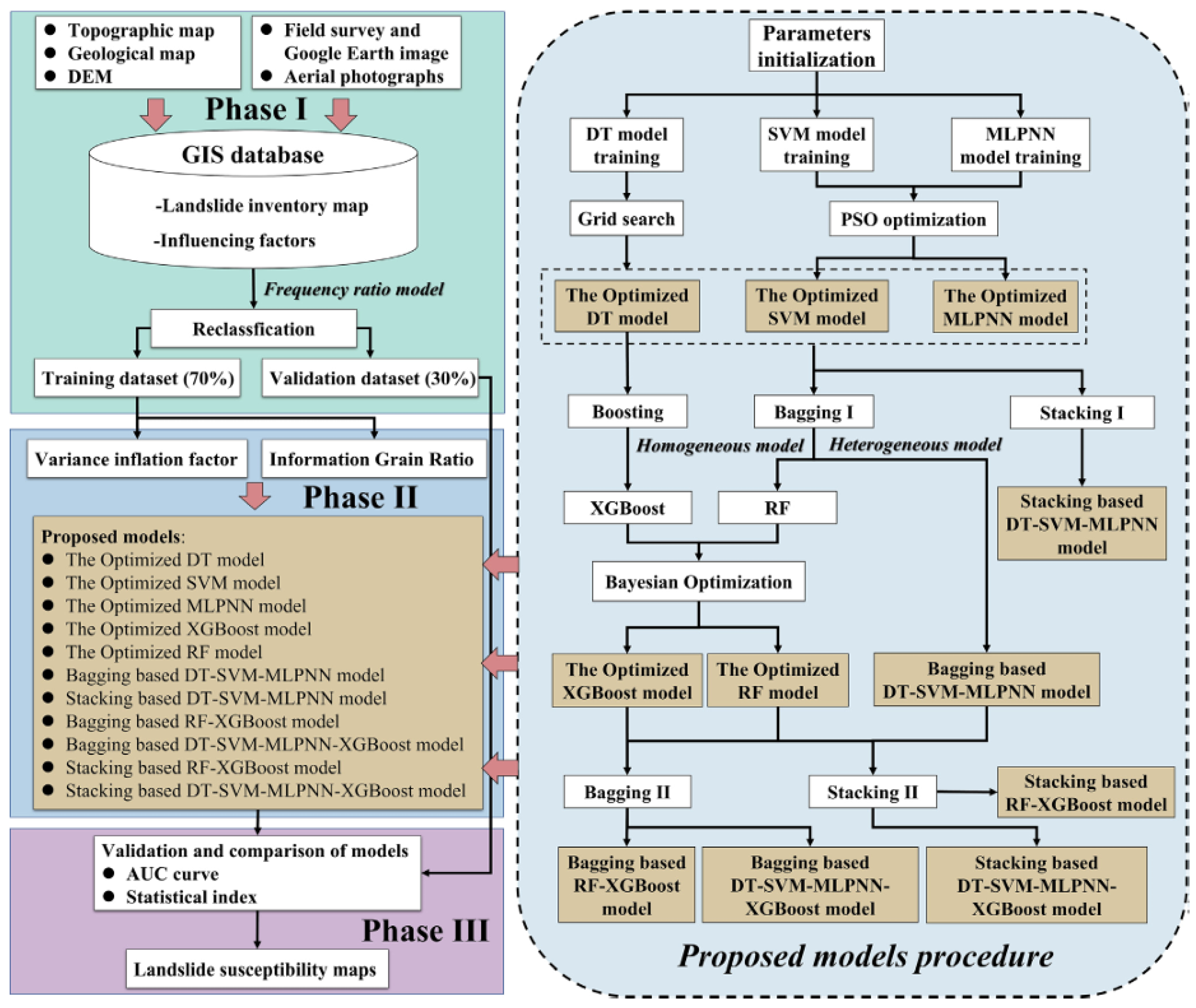
Zeng et al. [52] conducted an ensemble study at the township level, combining ML models with DL ensemble methods, integrating models like DT, SVM, and Multi-Layer Perceptron Neural Network (MLPNN) with RF and XGBoost. The flowchart of the combined methodology is illustrated in Figure 15 below. Their stacking-based RF-XGBoost model achieved the highest accuracy (AUC = 0.955), demonstrating the efficacy of combining traditional ML models with DL architectures. This hybrid approach allowed the model to capture complex spatial dependencies across Dazhou’s diverse terrain, showcasing DL ensembles’ potential to address LSM in heterogeneous landscapes.
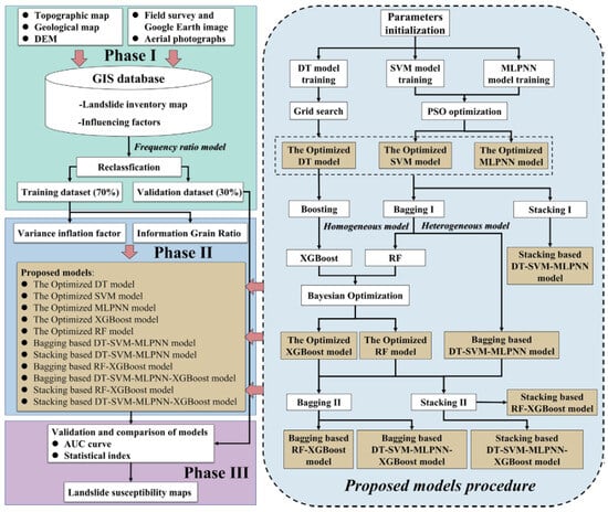
Figure 15.
Flowchart of the combined methodology for LSM development by Zeng et al. [52].
Ensemble models significantly improve LSM accuracy by integrating multiple algorithms’ strengths. ML ensembles are ideally suited for large-scale, adaptable mappings, while DL ensembles provide the depth and stability necessary for detailed, high-complexity susceptibility mapping in challenging terrains. By enhancing robustness and accuracy, these advanced ensemble approaches offer high-performance models adaptable to diverse LSM needs across varying geographic scales.
4.4. Hybrid Models
Hybrid models have become a leading approach in LSM, where combining multiple ML and DL techniques often yield superior predictive accuracy and adaptability. By leveraging the complementary strengths of different algorithms, hybrid models enhance the capacity to capture intricate spatial, temporal, and environmental relationships in LSM, especially in data-scarce or complex terrains. This section reviews recent advancements in hybrid models for LSM, categorizing approaches by their specific hybrid methods, targeted data types, and unique contributions to addressing LSM challenges.
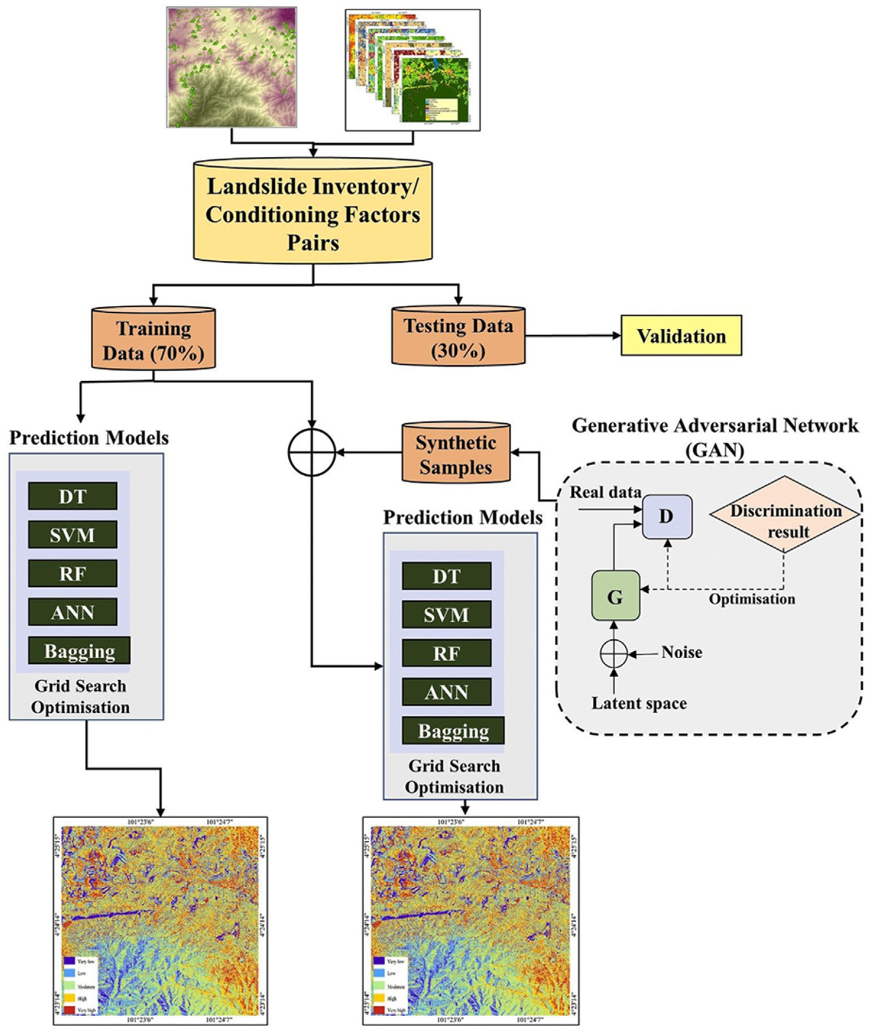
In regions with limited landslide data, hybrid models can compensate for data scarcity through data augmentation, transfer learning, or adaptive sampling. For example, Al-Najjar and Pradhan [26] employed generative adversarial networks (GANs) to generate synthetic data alongside various ML models, including DT, RF, and SVM, in the Cameron Highlands, Malaysia (Figure 16). By augmenting data, this GAN-based hybrid model achieved AUROC improvements across most models, with the GAN-RF combination reaching 0.94 on the training set and 0.82 on the test set. This demonstrates the utility of data synthesis in regions where landslide data collection is challenging, improving model performance without extensive field data.

Figure 16.
Flowchart of the study [26].
Similarly addressing data scarcity, Wang and Brenning [50] introduced the Unsupervised Active-Transfer Learning (UATL) framework, combining active learning with transfer learning for LSM in regions with limited labeled data. UATL uses adaptive sample selection to maximize information from minimal labeled data, achieving accuracy within 2% of models fully trained on target data. The UATL framework demonstrates effective sample selection, making it suitable for adaptive applications in LSM where data availability is restricted.
Chen et al. [61] proposed a meta-learning approach using block-wise analysis for LSM in large, heterogeneous regions with sparse data, such as Chongqing City, China. By dividing the region into blocks and applying meta-learning to adapt to local data, Chen et al. created a model that quickly adjusts to varied environmental factors across spatial blocks, particularly useful for large-scale regions where environmental heterogeneity and data limitations are common. This approach highlights the advantage of localized learning within hybrid models to adapt to complex landscapes with limited data.
In landslide-prone regions with complex spatial or temporal interactions, hybrid models that integrate DL architectures with advanced feature extraction methods can capture intricate dependencies across varied scales. In mountainous Mussoorie, India, Peethambaran et al. [20] applied ANN-based methods, specifically extreme learning machine (ELM) and the extreme learning adaptive neuro-fuzzy inference system (ELANFIS), achieving superior performance with ELANFIS. While the study did not provide a direct AUC, ELANFIS’s robust performance indicates ANN’s adaptability in complex terrains where variability in geomorphological factors is high. However, compared to DL models, ANN models in single-model approaches are limited by their need for careful parameter tuning, which can affect performance in more heterogeneous environments.
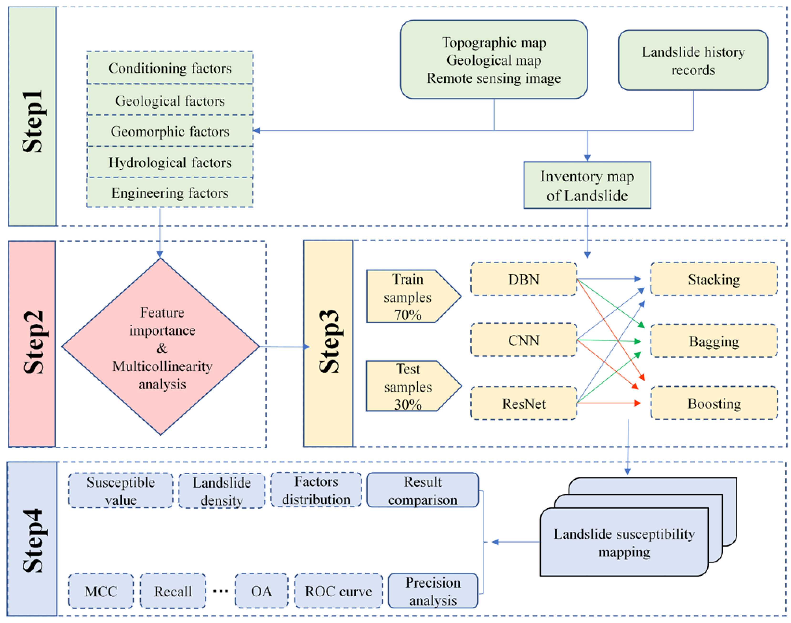
Lv et al. [36] developed a heterogeneous ensemble model (HEL) framework in the Three Gorges Reservoir area, China, combining DL models like deep belief network (DBN) and CNN with ensemble techniques, including Stacking and Boosting. The flowchart of the study is presented in Figure 17. Achieving an AUC of 0.984, this HEL framework demonstrated strong predictive performance, capturing spatially complex patterns in landslide susceptibility. By combining DL and ensemble techniques, HEL models provide a robust solution for areas with high variability in conditioning factors, ensuring stability and accuracy.
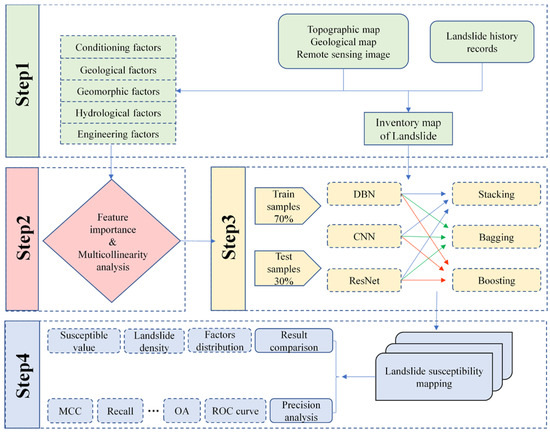
Figure 17.
Flowchart of the study [36].
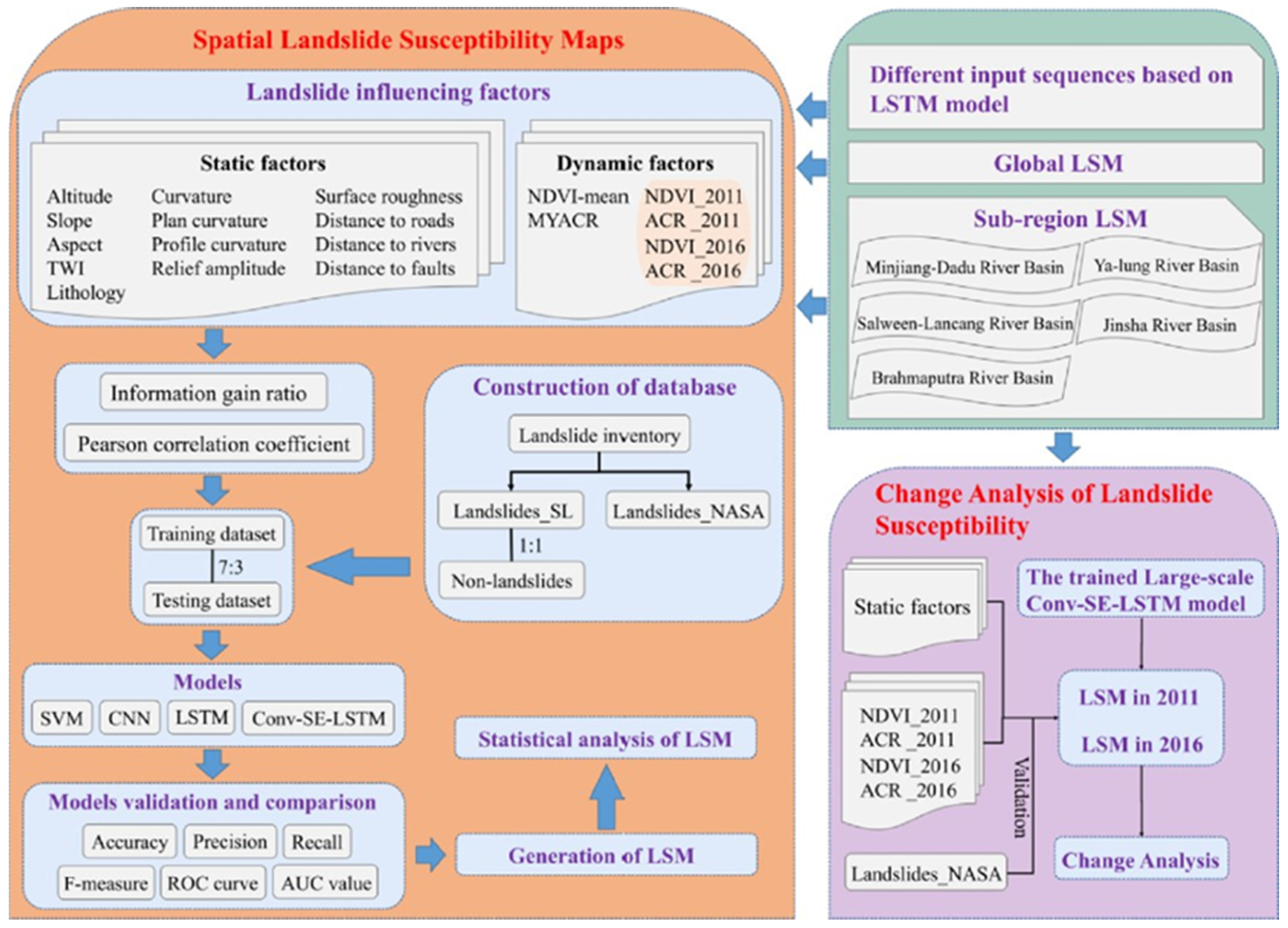
Similarly, Huang et al. [45] applied a hybrid Conv-SE-LSTM model in the Sichuan-Tibet corridor, combining Convolutional layers, Squeeze-and-Excitation networks, and Long Short-Term Memory layers to model sequential dependencies in LSM (Figure 18). This hybrid achieved an AUC of 0.8813, capturing dynamic relationships such as rainfall variation and vegetation cover, which influence landslide susceptibility. The Conv-SE-LSTM framework exemplifies how integrating DL with sequence modeling can address temporal dependencies, making it well suited for regions with dynamic environmental factors.
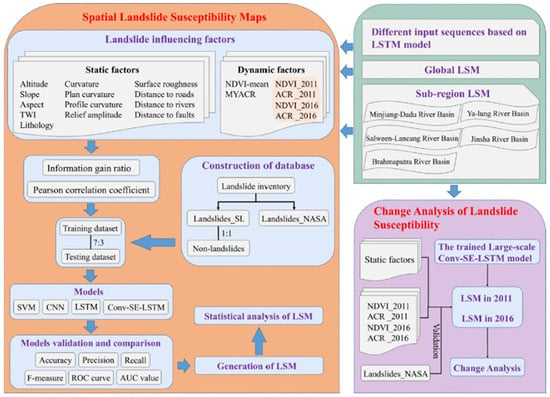
Figure 18.
Flowchart of the research work conducted by Huang et al. [45].
Li et al. [34] introduced the GL-ResNet model in Wenchuan, China, combining ResNet blocks for feature extraction with LSTM layers for sequence learning, supplemented by GoogLeNet blocks to broaden perceptual fields. Achieving an AUC of 0.96, GL-ResNet captured both spatial and temporal dependencies, proving highly effective in mountainous terrains with complex geomorphological features. This model exemplifies how combining DL architectures can enhance feature extraction across multiple scales, a critical capability for LSM in topographically diverse landscapes.
High-dimensional data, common in LSM due to the range of conditioning factors (e.g., lithology, rainfall, topography), often requires hybrid models to efficiently handle and reduce data complexity. Wei et al. [37] designed the spatial response—machine learning (SR-ML) framework (Figure 19), a hybrid that integrates Depthwise Separable Convolution for dimensionality reduction and ML classifiers for final prediction, applied in the Yarlung Zangbo Grand Canyon. Achieving an AUC of 0.92, the SR-ML framework demonstrated how feature extraction through convolutional layers can improve model performance, especially in spatially complex environments where feature dimensions are high.
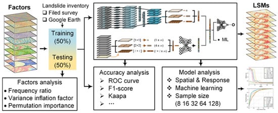
Figure 19.
Flowchart of SR-ML framework [37].
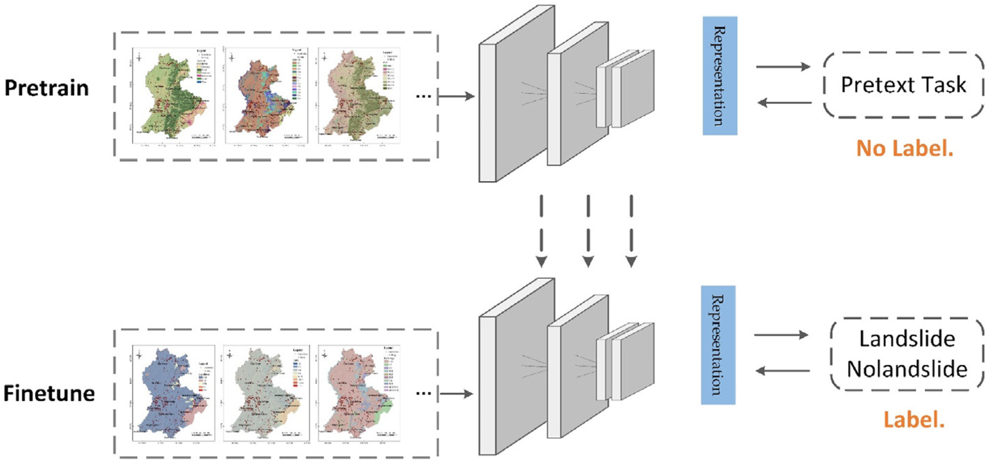
Chang et al. [40] developed a hybrid model that combines FR and TabNet with RF as a baseline in Lvliang City, China. The hybrid RF-TabNet (Figure 20) model achieved higher sensitivity and specificity compared to traditional methods, with rainfall emerging as the most significant predictor for landslide occurrence. This hybrid approach illustrates the potential of integrating feature selection and DL for effective high-dimensional data handling in LSM, particularly in densely vegetated or variable terrain.
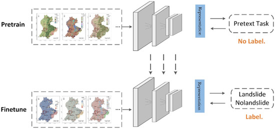
Figure 20.
Schematics of self-supervised learning process in TabNet [40].
Similarly, Liao et al. [35] applied a hybrid approach combining Spearman correlation coefficient and recursive feature elimination to optimize feature selection across varying grid resolutions in Chongqing, China. By fine-tuning conditioning factors across resolutions, the hybrid spearman correlation coefficient–recursive feature elimination (SCC-RFE) model achieved higher precision, sensitivity, and AUC, emphasizing the need for adaptive feature selection methods when handling high-dimensional data in LSM.
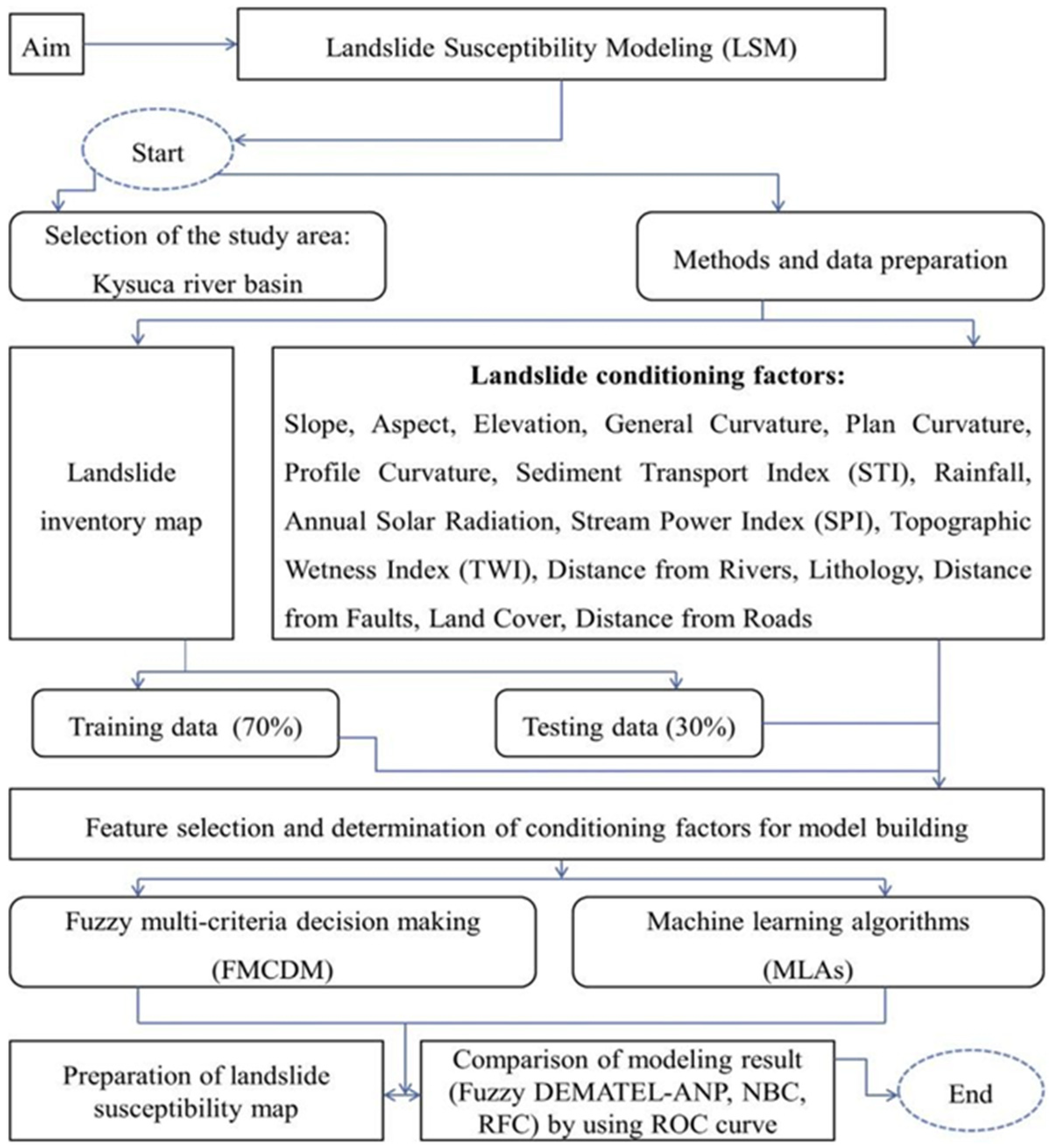
Another classification of region-specific hybrid models often incorporates local topographical, hydrological, or geological insights to improve susceptibility mapping in targeted landscapes. Ali et al. [25] applied a FDEMATEL-ANP approach with ML classifiers like Naïve Bayes and RF (Figure 21) in Slovakia’s Kysuca River basin, achieving an AUC of 95.4%. The integration of fuzzy decision-making with ML provided a nuanced understanding of local conditioning factors, demonstrating that hybrid models can capture region-specific risks effectively.
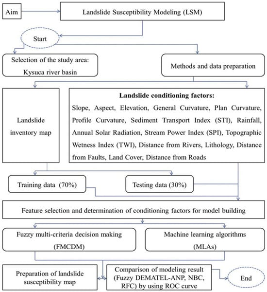
Figure 21.
Flowchart of the adopted methodology by Ali et al. [25].
In Uttarkashi, India, Kainthura and Sharma [33] evaluated five hybrid models that combined the Rough Set theory with ML models such as Bayesian networks and XGBoost. The XGBoost-Rough Set hybrid achieved the highest accuracy (89.92%), underscoring the advantage of hybrid models in regions with distinct geomorphological conditions where correlations among conditioning factors may be unique.
In earthquake-prone areas, Han et al. [43] proposed a KDE-MDBN (Kernel Density Estimation–Multi-Dependent Bayesian Network) model for post-earthquake LSM. This hybrid achieved an AUC of 0.916 by incorporating kernel density estimation to capture spatial clustering effects, making it highly suitable for regions with high landslide density following seismic events. The KDE-MDBN model effectively integrates spatial hazard assessment with Bayesian network capabilities, offering a robust solution for earthquake-affected areas.
For large-scale assessments, hybrid models often integrate multiple classifiers to improve generalizability and adaptability across extensive or diverse terrains. Rong et al. [48] combined integrated ML models with scenario simulations to project landslide susceptibility in Shuicheng County, China. By factoring in extreme precipitation and socioeconomic scenarios, the model provided a multi-dimensional risk assessment, achieving an AUC of 0.85. This comprehensive approach highlights the value of combining susceptibility modeling with future risk scenarios, aiding long-term planning in disaster-prone areas.
Hong et al. [44] utilized Locally Weighted Learning (LWL) combined with classifiers such as Radial Basis Function (RBF) and Credal Decision Trees (CDT) in Yongxin County, China. The hybrid LWL-RS-CDT model achieved the highest ROC AUC of 0.996, demonstrating that combining adaptive learning with multiple classifiers can significantly enhance LSM accuracy, especially for large-scale applications where adaptability across varied terrains is crucial.
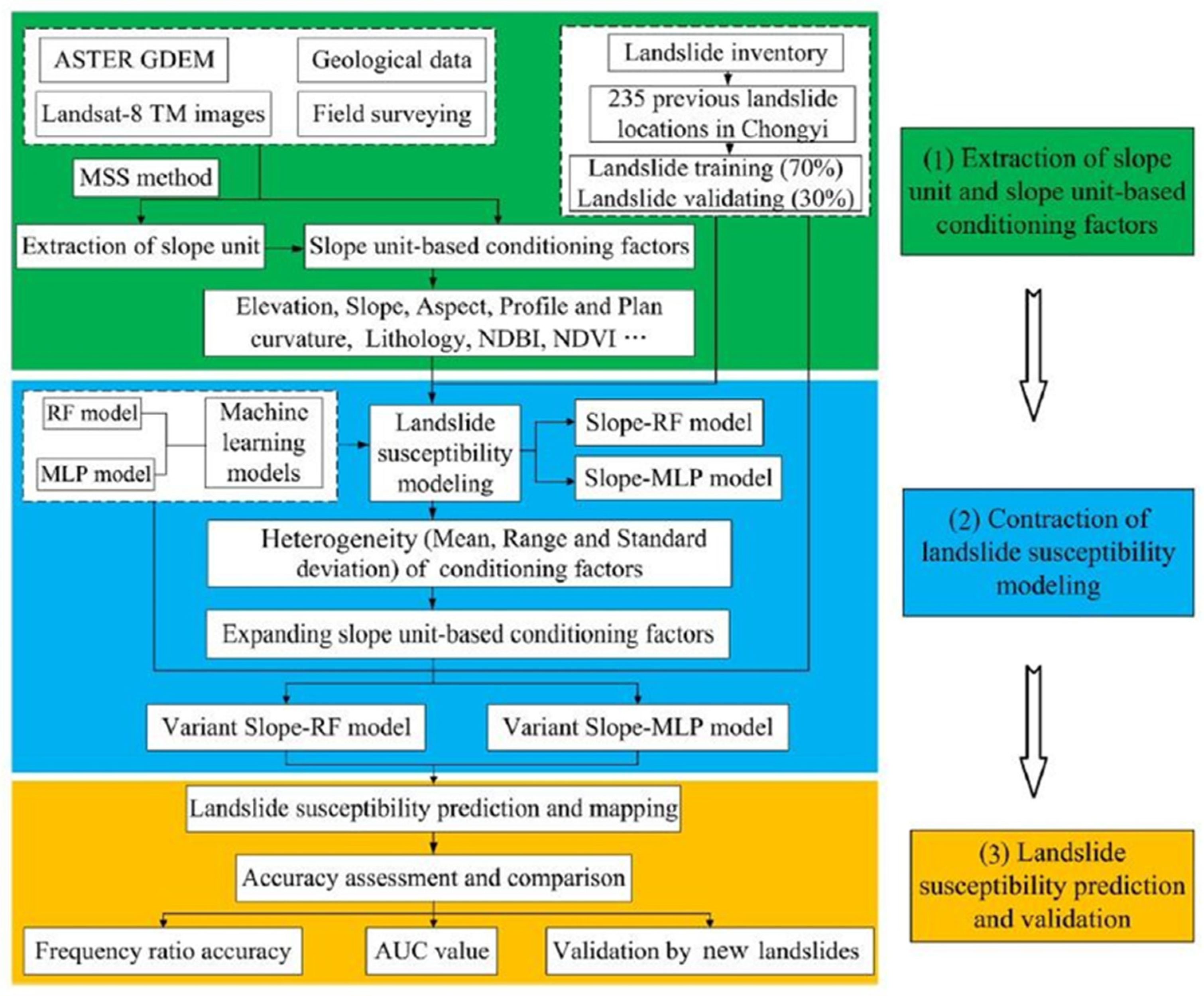
In Lvliang City, China, Chang et al. [41] applied slope-based RF and MLP models, achieving high accuracy in landslide susceptibility prediction by using slope units for terrain segmentation. The hybrid Slope-RF and Slope-MLP (Figure 22) models achieved AUC values of 0.875 and 0.805, respectively, showing that integrating ML with terrain-specific units allows for more accurate susceptibility mapping, particularly in mountainous regions where landslide risk varies significantly with slope characteristics.
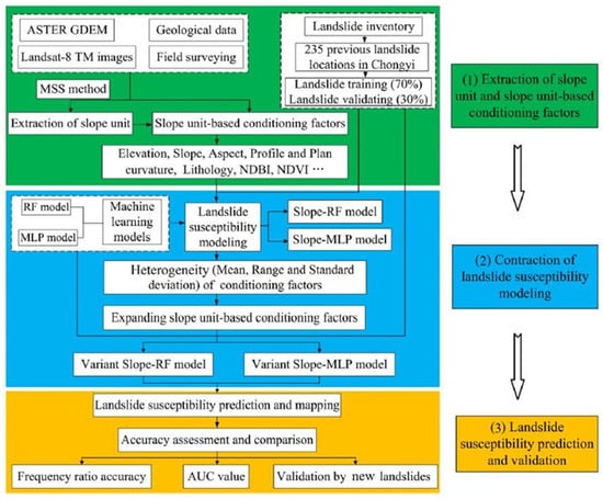
Figure 22.
Flowchart for variant slope-based ML models used by Chang et al. [41].
In a recent study, Haoyuan Hong [54] developed five integrated models for LSM in Yongxin County, China, by combining Locally Weighted Learning (LWL) with various ML algorithms, including Radial Basis Function (RBF), Fisher’s Linear Discriminant (FLDA), Quadratic Discriminant Analysis (QDA), Credal Decision Tree (CDT), Alternating Decision Tree (ADT), and Random Subspace (RS). The integration of LWL with these algorithms demonstrated strong predictive capabilities, with the LWL-RS-CDT model achieving the highest ROC AUC value of 0.996, followed closely by LWL-RS-ADT at 0.975. Using data from 364 landslide locations and 15 environmental factors, the study highlighted the importance of NDVI, lithology, and altitude as key predictors. This hybrid approach showcases the effectiveness of combining LWL with multiple ML techniques, providing a robust framework for LSM and enhancing predictive accuracy beyond traditional models such as SVM, Naive Bayes (NB), and Logistic Regression (LR)
Overall, hybrid models demonstrate diverse strengths in LSM, providing solutions for different challenges such as data scarcity, high-dimensional data, complex spatial–temporal patterns, and regional specificity.
- Data-Scarce Regions: GAN-based hybrids and UATL frameworks show effectiveness in regions with limited data, with GANs enhancing data representation and UATL providing adaptive learning capabilities.
- Complex Spatial–Temporal Patterns: DL-based hybrids such as HEL and Conv-SE-LSTM excel in capturing intricate spatial and temporal dependencies, making them highly effective for dynamic landscapes influenced by variable factors like rainfall and vegetation cover.
- High-Dimensional Data: Hybrid models with convolutional layers (e.g., SR-ML) or feature selection (e.g., SCC-RFE) efficiently manage high-dimensional datasets, enhancing predictive power in terrains with a broad range of conditioning factors.
- Region-Specific Models: Models like FDEMATEL-ANP and KDE-MDBN are effective for region-specific analyses, providing tailored insights that capture local environmental factors or post-disaster conditions, especially useful in targeted or unique geographic settings.
Hybrid models in LSM offer robust, context-sensitive solutions for diverse geographic and environmental landscapes. By merging ML and DL techniques, these models address limitations in single-model approaches and provide advanced frameworks capable of handling complex data, ensuring reliable predictions for disaster risk reduction and land use management. The varied applications of hybrid models underscore their transformative impact on landslide susceptibility mapping, enabling improved accuracy and resilience in assessments across both large-scale and localized terrains.
5. Conclusions
AI models are actively being developed to predict landslide susceptibility and mapping them for the selected geographical locations. With more powerful methods and data availability, such solutions are becoming more robust and reliable. In the current studies, the research works published since 2020 are reviewed. This work provides a comprehensive classification of AI models in landslide susceptibility mapping, illustrating how Single-Model Approaches, Enhanced Models with Optimization, Ensemble Models, and Hybrid Models contribute to predictive accuracy, adaptability, and robustness in varied geographic and data conditions. Given the critical importance of landslide mapping for safeguarding lives and infrastructure, this work serves as a resource for researchers, practitioners, and policymakers aiming to leverage AI in their risk mitigation efforts. The practical implications of each model category:
- Single-model approaches provide essential baseline insights into landslide susceptibility patterns using models such as RF, SVM, and CNN. These models are highly accessible, offering a straightforward approach for initial assessments in LSM. However, their predictive power is often limited in complex terrains or when handling imbalanced datasets, underscoring the need for more advanced methods in challenging environments.
- Enhanced models with optimization improve upon single models by addressing specific limitations through techniques like Bayesian optimization, class weighting, and transfer learning. Such models excel in scenarios with data imbalance or data scarcity, offering greater adaptability and precision. In areas with uneven data distributions or where new data collection is limited, these optimized models deliver substantial improvements in predictive reliability, making them valuable tools for LSM in structured and data-limited regions.
- Ensemble models aggregate the strengths of multiple algorithms to capture complex spatial patterns that single models may overlook. Techniques such as stacking, bagging, and blending create robust predictive frameworks that perform well across diverse and variable terrains. These ensemble methods excel in large-scale assessments, where achieving high stability and consistency is essential for accurate, broad-area LSM. By combining different models, ensemble methods increase resilience against environmental variability, establishing themselves as reliable choices for both national and regional assessments.
- Hybrid models represent the most flexible and powerful approach, integrating ML and DL techniques or combining ensemble and optimization strategies to achieve high adaptability. These models are especially effective in high-dimensional and data-rich environments, where capturing intricate relationships between conditioning factors is essential. Hybrid models address the limitations of single, optimized, and ensemble models by blending multiple approaches, providing a balanced combination of predictive power and robustness. This versatility makes hybrid models particularly suited for high-stakes applications where precision is paramount, such as in regions prone to frequent landslides or complex geomorphological features.
This classification framework allows researchers and practitioners to align model complexity with specific LSM requirements, balancing factors such as computational cost, data quality, and the intricacies of terrain. Each category serves a distinct purpose, with single models offering initial assessments, optimized models enhancing accuracy in specific data conditions, ensemble models boosting resilience, and hybrid models providing advanced adaptability for the most demanding landscapes.
While these developments have led to significant progress, several challenges remain. The availability and quality of data are crucial to further improving the reliability of AI models, and future efforts should focus on expanding access to high-quality datasets, such as high-resolution satellite imagery. Additionally, handling data imbalances and improving generalization across diverse geographic regions remain ongoing issues, which could be addressed through techniques like transfer learning and data augmentation. Another promising avenue is the integration of AI models with real-time monitoring systems, enabling dynamic updates to landslide susceptibility maps and providing early warnings in high-risk areas. Future research should explore multi-hazard frameworks that account for interactions between landslides and other natural disasters, as well as incorporating explainable AI (XAI) techniques to enhance model transparency and trust. Interdisciplinary collaboration between geologists, data scientists, and hydrologists, as well as international cooperation for dataset sharing, will also be key to further advancing the field. Overall, this review aims to provide guidance for researchers and practitioners in developing AI-based landslide susceptibility mapping solutions, while highlighting recent advancements and future directions for innovation.
Author Contributions
Conceptualization, M.K., S.N. and G.I.; software, B.I., Y.M. and B.A.; formal analysis, E.O. and N.S.; investigation, M.K., S.N. and B.I.; resources, B.A. and N.S.; writing—original draft preparation, M.K., Y.M. and B.A.; writing—review and editing, S.N., B.I., B.A. and E.O.; visualization, Y.M. and N.S.; supervision, M.K. and S.N.; project administration, M.K. and N.S.; funding acquisition, S.N. All authors have read and agreed to the published version of the manuscript.
Funding
This research was funded by Science Committee of the Ministry of Science and Higher Education of the Republic of Kazakhstan, grant number BR24992865. The APC was funded by the projects budget. This research was implemented with a focus on the partial requirements of PhD Candidate Muratbek Kudaibergenov’s doctoral dissertation on the “Geodetic substantiation of geoecological zoning of the territory according to the degree of danger of gravitational processes” at the department of Cartography and Geoinformatics, Farabi university, Almaty, Kazakhstan.
Data Availability Statement
Data are contained within this article.
Acknowledgments
We are grateful to all the authors of the articles that were discussed in this review.
Conflicts of Interest
The authors declare no conflicts of interest.
Appendix A
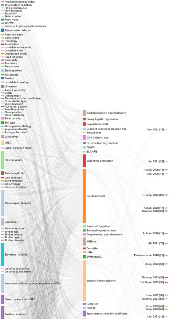
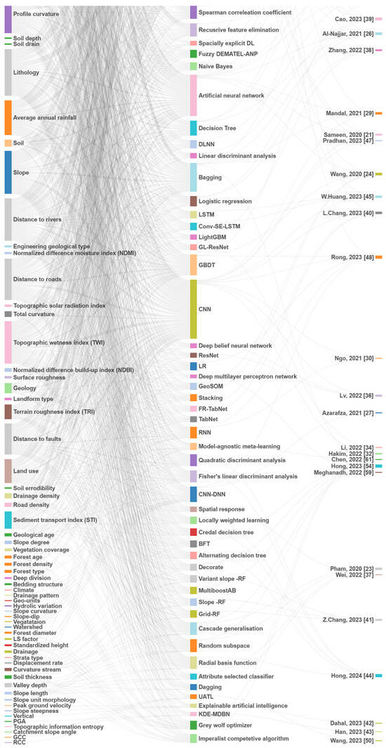
Figure A1.
Sankey diagram to demonstrate the application of AI models on LSM [16,17,18,19,20,21,22,23,24,25,26,27,28,29,30,31,32,33,34,35,36,37,38,39,40,41,42,43,44,45,47,48,49,50,51,52,53,54,55,56,59,61].
Figure A1.
Sankey diagram to demonstrate the application of AI models on LSM [16,17,18,19,20,21,22,23,24,25,26,27,28,29,30,31,32,33,34,35,36,37,38,39,40,41,42,43,44,45,47,48,49,50,51,52,53,54,55,56,59,61].

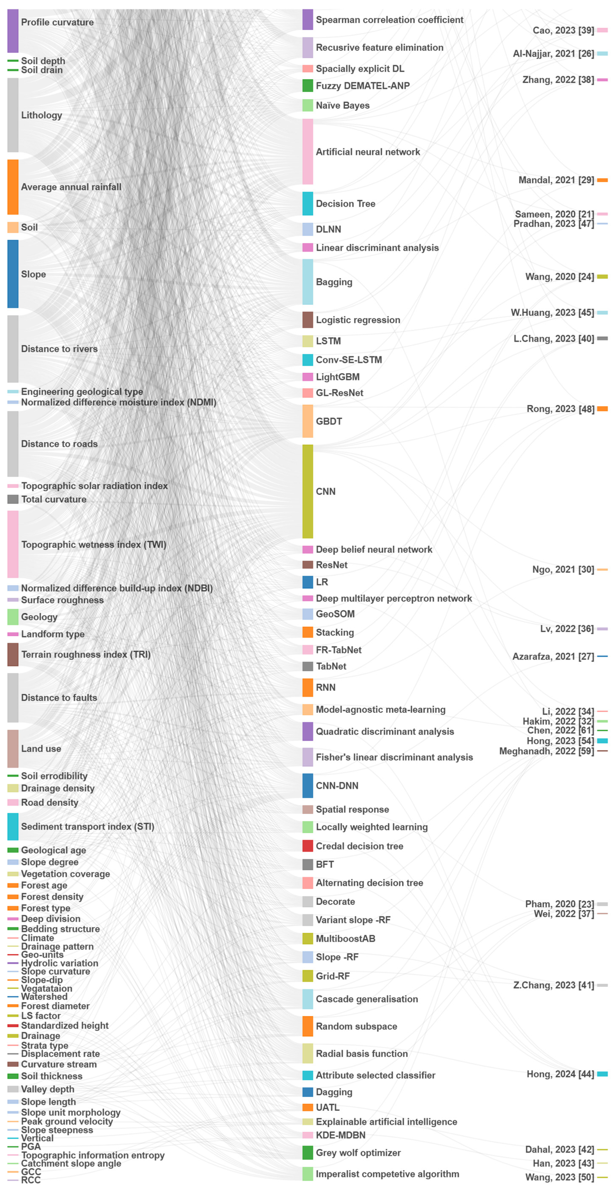

Table A1.
Summary of research works in chronological order.
Table A1.
Summary of research works in chronological order.
| Publication Year, Authors | Geographic Location | Combined AI Model? (Y/N) | AI Models | Geological/Weather Information | Selected Parameters for Models | Software Used to Develop Models | Data Size | Accuracy | ||||||
|---|---|---|---|---|---|---|---|---|---|---|---|---|---|---|
| Altitude Range (Sea Level) | Slope Angle | Mean Annual Precipitation | Mean or Max/Min Temperature | |||||||||||
| Achour et al., 2020 [16] | A1 highway at Ain Bouziane, North-East of Algeria | No |
| 226 to 718 m | 0° to 46° | 556 mm | 7 °C and 37 °C, max/min |
| R software; ArcGIS | 1871 landslide pixels: 70% training; 30% testing. | AUC of models: RF: 0.972 SVM: 0.856 BRT: 0.760 | |||
| Adnan et al., 2020 [17] | Cox’s Bazar district, South-East of Bangladesh | Yes |
| 18 m | 0° to 59° | 4288 mm | - |
| - | 1262 sample locations (670 landslide and 592 non-landslide): 60% training; 40% testing. | RF: 96.63% MLP: 95.45% SVM: 94.06% KNN: 90.69% Combined method: 97% | |||
| Dao et al., 2020 [18] | Muong Lay district, Dien Bien province, Vietnam. | No |
| 125 to 1778 m | 0° to 73° | 1483 mm | 22–23 °C, mean |
| Open-source WEKA software | 217 landslides: 70% training; 30% testing. | AUC and accuracy of training: QDA: 0.881 and 81.67% FLDA: 0.867 and 81.46 MLP: 0.901 and 86.42% DL: 0.899 and 81.85% AUC and accuracy of validation: QDA: 0.806 and 72.31% FLDA: 0.860 and 79.21% MLP: 0.841 and 76.15% DL: 0.887 and 82.31% MLP: 0.841 and 76.15% DL: 0.887 & 82.31% | |||
| Huang et al., 2020 [19] | Shicheng County, China | No |
| 0 to 1320 m | 3.9° to 19.1° | 1885 mm | - |
| - | 369 landslides: 70% training; 30% testing | AUC of models:
| |||
| Peethambaran et al., 2020 [20] | Mussoorie Township, Dehradun, India | No |
| 654 to 2253 m | 0° to 72.5° | 155 mm | - |
| MATLAB | 49 landslides: 70% training; 30% testing. | AUC of models:
| |||
| Sameen et al., 2020 [21] | Southern Yangyang Province, South Korea | No |
| −5.88 to 929.79 m | 0° to 79° | - | - |
| Python using Scikit-Learn and Keras | 219 landslides: 70% training; 30% testing. | Accuracy and AUC of training:
| |||
| Tien Bui et al., 2020 [22] | Kon Tum Province, Vietnam | No |
| 136.8 to 2580.2 | 0° to 72.5° | 1700–3000 mm | - |
| WEKA software, Python, ArcGIS | 1657 landslides: | Accuracy (%) of training:
| |||
| Pham et al., 2020 [23] | Van Chan district, Yen Yen Bai Province, Vietnam | No |
| 60 m to 2542 m | 0° to 84.2° | - | - |
| WEKA software ArcGIS 10.3 | 167 landslides: 70% training; 30% testing. | AUC of Training:
| |||
| Wang et al., 2020 [24] | Zhejiang Province, China | Yes |
| −58 to 1879 m | 0° to 52.4° | 1100—2000 mm | 15 °C to 18 °C |
| GeoSOM, scikitlearn Python | 1051 landslide samples: 70% training; 30% testing. | Training accuracy:
| |||
| Ali et al., 2021 [25] | Kysuca river basin, Slovakia | No |
| 326 to 1226 m | 0° to 63.14° | 800 to 1500 mm | - |
| 2000 landslide and non-landslide 70% training, 30% testing | AUC: Fuzzy DEMATEL-ANP = 0.924 RF = 0.954 NB = 0.909 | ||||
| Al-Najjar, 2021 [26] | Cameron Highlands, Pahang state, Malaysia | GAN is usedto createadditionaldata |
| 840 to 2110 m | 0° to 78.88° | - | 14 °C at night, 24 °C during the day |
| 156 landslides, 70% training, 30% testing 222 landslides 80% training, 20% testing | Before GAN method, AUROC values for training/test were: DT: 0.90/0.76 RF: 0.94/0.81 SVM: 0.86/0.85 ANN: 0.69/0.72 Bagging ensemble: 0.82/0.75 After GAN method: DT: 0.92/0.78 RF: 0.94/0.82 SVM: 0.88/0.82 ANN: 0.75/0.78 Bagging ensemble: 0.84/0.8 | ||||
| Azarafza et al., 2021 [27] | Isfahan province, Iran | Yes |
| 1211 to 2560 m | 116.9 mm on average | Min and max: 10.6 °C and 40.6 °C Average: 16.7 °C |
| ArcGIS 10.4 to produce landslide susceptibility maps | 90.9% AUC; 84.8% IRs; 0.17 MSE 0.40 RMSE 0.42 MAPE | |||||
| Liu et al., 2021 [28] | Kvam region, Norway | Yes |
| 250 to 1190 m | 500 mm | Mean temperature 3.3 °C |
| 10,197 location points 70% training, 30% testing | AUC values: RF = 0.99 GBRT = 0.99 MLP = 0.97 | |||||
| Mandal et al., 2021 [29] | Rorachu river basin of Sikkim Himalaya, India | No |
| 786 to 4062 m | 75.24° | From 510 to 2240 mm | Mean temperature 22 °C—summer, 4 °C—winter |
| - | 214 landslides 70% training, 30% testing | AUC values for training: CNN = 0.903 RF = 0.9 ANN = 0.897 Bagging = 0.881 For testing: CNN = 0.939 RF = 0.925 ANN = 0.925 Bagging = 0.915 | |||
| Ngo et al., 2021 [30] | Iran | No |
| −10 to 4500 m | 0° to 60° | 450–1800 mm in West, North 100–300 mm in East, South | - |
| ArcGIS 10.2 to generate non-landslide locations for training and testing | 4069 Landslides 70% training, 30% testing | RNN: 85% AUC CNN: 88% AUC | |||
| Gao et al., 2021 [31] | Zigui County Yichang, Hubei, China Jiuzhaigou County, Sichuan Province, China | No |
| Site-1: 80 to 1220 m Site-2: 2268 to 4114 m | Site-1: 0° to 62.69° Site-2: 0° to 67.57° | - | - |
| Python: TensorFlow | Site-1: 74 landslides Site-2: 124 landslides. Data augmentation was used to increase data amount | Site-1:
| |||
| Gameiro et al., 2021 [57] | Serra Geral, southern Brazil. | No |
| Up to 1400 m | - | - | - |
| Matlab | 1638 landslide and 1638 non- landslide data points:
| Single model global accuracy:
| |||
| Soares et al., 2022 [58] | Nova Fribugo (Train area [TA]1) and Teresopolis (TA2) in Rio de Janeiro (RJ); and Rolante (TA3) in Rio Grande do Sul (RS), Brazil | No |
| RJ: 1100 and 2000 m RS: 19 to 997 m | RJ: 1585.62 mm RS: 1700 and 2000 mm | - |
| Tensorflow 2.0 Python Deep learning framework | TA1: 497 landslides TA2: 117 landslides TA3: 110 landslides | Precision: TA1 = 0.47 TA2 = 0.5 TA3 = 0.56 | ||||
| Chen et al., 2022 [61] | 1) Fengjie County (FJ) 2) Fuling District (FL) Both in Chongqing City, China |
| 0° to 88.32° | - | - |
| Accuracy: For FJ: RF = 74.8% RL = 74.9% MAML = 72.6% For FL: RF = 77.8% RL = 81.6% MAML = 76.4% | |||||||
| Hakim et al., 2022 [32] | Icheon City, South Korea | Yes |
| 25 to 710 m | 0° to 76° | 1234 mm | 24 °C and 7 °C |
| 456 landslides 70% training, 30% testing | Only CNN: AUC = 0.847 RMSE = 0.12 CNN-GWO: AUC = 0.876 RMSE = 0.08 CNN-ICA: AUC = 0.852 RMSE = 0.09 | ||||
| Kainthura, 2022 [33] | Uttarkashi, India | Yes |
| 920 to 3830 m | 0° to >35° | 1902 mm | - |
| ArcGis to generate study area | 373 landslide and 181 non- landslide 75% training; 25% testing | AUC for training: HBNRS = 0.897 HBPNNRS = 0.977 HBRS = 0.995 HXGBRS = 0.996 HRFRS = 0.989 AUC for testing: HBNRS = 0.883 HBPNNRS = 0.924 HBRS = 0.894 HXGBRS = 0.937 HRFRS = 0.904 | |||
| Li et al., 2023 [34] | Wenchuan area, China | Yes |
| 763 to 5827 m | 0° to >40° | Annual rainfall ranging from 528.7–1332.2 mm | Average annual temperature: 13.5 °C–14.1 °C |
| 1147 landslides 70% training, 30% testing | AUC for training: GL-ResNet = 0.98 Res-Net = 0.97 SVM = 0.95 DBN = 0.95 GRU = 0.94 LR = 0.92 AUC for testing GL-ResNet = 0.96 Res-Net = 0.95 SVM = 0.94 DBN = 0.95 GRU = 0.94 LR = 0.92 | ||||
| Liao et al., 2022 [35] | Wushan and Wuxi, Chongqing, China | Yes |
| 0 to >2500 m | 0° to 41.54° | - | - |
| ArcGIS | 1137 landslides 70% training; 30% testing | AUC for grid size of 2000 m: RF = 0.98 SCC-RF = 0.94 RFE-RF = 0.92 SCC-RFE-RF = 0.96 | |||
| Lv et al., 2022 [36] | Zigui and Badong county, Hubei province, China | Yes |
| 80 to 2000 m | 0° to 78.419° | 1100 mm | - |
| 202 landslides 70% training, 30% testing | AUC: DBN = 0.956 CNN = 0.976 ResNet = 0.981 Stacking = 0.984 SA = 0.979 WA = 0.979 Boosting = 0.982 | ||||
| Meghanadh et al., 2022 [59] | Alaknanda river, Srinagar- Rudraprayag area, Uttarakhand state, India |
| 634 to 1764 m | 21° to 70° | - | - |
| ROC_AUC: Proposed model = 0.9072 Random forest = 0.9099 Support vector machine = 0.8992 | ||||||
| Wei et al., 2022 [37] | Yarlung Zangbo Grand Canyon region, Nyingchi, Tibet Autonomous Region | No |
| 324 to 7782 m | 0° to 89° | 605 to 1903 mm | - |
| ArcGIS, Python | 203 landslides 50% training, 50% testing | AUC: SR = 0.92 SR-ML = 0.91 | |||
| Zhang et al., 2022 [38] | Wanzhou District, Chongqing Municipality, Three Gorges Reservoir | No |
| 26 to 1006 m | 0° to 65.125° | 1132.39 to 1192.74 mm | - |
| 233 landslides 60% training, 40% testing | AUC: LR = 0.835 LightGBM = 0.89 RF = 0.844 | ||||
| Cao et al., 2023 [39] | Western Henan Province, China | No |
| 12–2387 m | 0° to 76° | 700–900 mm | 13.8°C |
| - | 256 landslides: 70% training; 30% testing. | Training AUC: RF: 1.00 XGBoost: 1.00 SVM: 0.98 LDA: 0.89 LR: 0.87 Testing AUC: XGBoost: 0.8759 RF: 0.8743 LDA: 0.8685 LR: 0.8624 SVM: 0.7666 | |||
| Chang et al., 2023 [40] | Lvliang City, Western Shanxi, China | No |
| 552–2768 m | 0° to 35° | 450–510 mm | - |
| TabNet, ArcGIS | 3476 landslides: 80% training; 20% testing. | Accuracy (%):
| |||
| Zhilu Chang et al., 2023 [41] | Chongyi County, China | No |
| 142–1998 m | 0°–47.8° | 1615.2 mm | - |
| - | 744 landslides: 70% training; 30% testing. | AUC of models:
| |||
| Dahal and Lombardo, 2023 [42] | Gorkha, Nepal | No |
| 500–7000 m | - | - |
| r.slopeunits; Python | 24,903 coseismic landslides: 70% training; 30% testing. | AUC performance:
| ||||
| Han et al., 2023 [43] | Wenchuan county, China | No |
| 490–5600 m | - | - | - |
| ArcGIS, Python | 1336 sample points (668 landslide, 668 non- landslide): 70% training; 30% testing. | AUC of training: KDE-MDBN: 0.978AUC of testing:
| |||
| Hong, 2023 [44] | Yongxin County, China | Yes |
| 41–1389 m | 0°–67.6° | Average—1530.7 mm | Mean—18.2 °C |
| ArcGIS, SPSS, Matlab | 728 sample points (364 landslide, 364 non- landslide): 70% training; 30% testing. | AUC of training:
| |||
| Wubiao Huang et al., 2023 [45] | Sichuan-Tibet, China | No |
| 200 to 8589 m | 0°–89.4° | Annual cumulative rainfall: 288.49 to 2288.1 mm | - |
| Python: Scikit- learn and PaddlePaddle2.0 | 1669 landslide events: 70% training; 30% testing. | AUC of models:
| |||
| Faming Huang et al., 2023 [56] | Yanchang County, China | No |
| 473–1369 m | 0°–50° | 564 mm | - |
| ArcGIS, SPSS, R | Grids size/special resolution, m:
| AUC of models with training portion of dataset:
| |||
| Mondini et al., 2023 [46] | Italy | No |
| - | - | Cumulated rainfall: 1 mm ≤ E ≤ 2070 mm | - |
| CTRL–T; Tensorflow; Python. | 2472 rainfall- induced landslides: 80% training; 20% testing. | Training and validation accuracy:
| |||
| Pradhan et al., 2023 [47] | CheongJu region, South Korea | No |
| 20–655 m | 0° to 78° | >1200 mm | - |
| - | 519 landslides: 70% training; 30% testing. | Accuracy:
| |||
| Rong, 2023 [48] | Shuicheng County, China | Yes |
| 633–2863 m | 940–1450 mm | - |
| Python, keras, scikit | 480 | AUC and accuracy of the best integrated model:
| ||||
| Saha et al., 2023 [49] | Garhwal Himalaya, India | No |
| 1500–2500 m | - | - | - |
| ArcGIS | >3000 landslide points | AUC of testing: SVM: 0.845 RF: 0.874 Bagging: 0.906 ANN: 0.887 DLNN: 0.925 | |||
| Wang and Brenning, 2023 [50] | Source: Reuleut, Indonesia Target: Palu, Indonesia. | Yes |
| Source: up to 1851 m Target: 202 to 2331 m | Mean slope: Source: 13.2°. Target: 24.6° | - |
| R software | 507 landslides samples in source area 320 landslides in target area | pAUROC: 0.096 | ||||
| Yang et al., 2023 [51] | Anhua County, China | No |
| 202–2331 m | 0° to 71.7° | 986–2440 mm | Mean—16.2 °C |
| ArcGIS | 492 landslide samples | AUC of models:
| |||
| Zeng et al., 2023 [52] | Dazhou Town, China | Yes |
| >146 m <660 m | 0° to 74° | 1188.7 mm | - |
| ArcGIS Python | 78,529 landslide units. 78,529 non-landslide units. 70% training; 30% testing. | Stacking based RF- XGBoost—AUC 0.955 (the best model) | |||
| Zhiyong, 2023 [53] | Zigui Basin, China | Yes |
| <2008 m | 0° to 86° | 1250 mm | 13 °C |
| Python | 520 training set, 113 test set | AUC of models:
| |||
| Hong, 2024 [54] | Yongxin, China | Yes |
| 41–1389 m | 79% of area has slope less than 24° | 1530.7 mm | 18.2 °C |
| Matlab Weka ArcGIS | 364 landslide point data 364 non- landslide point data | AUC of training:
| |||
| Sharma et al., 2024 [55] | Political boundary of India | Yes |
| - | - |
| The final dataset had 1,282,908 data points with 641,454 of landslide and non-landslide points. The testing data contains 15,000 landslide points and 300,000 non- landslide points. | Ensemble—ROC AUC—0.989 | ||||||
References
- Li, B.V.; Jenkins, C.N.; Xu, W. Strategic Protection of Landslide Vulnerable Mountains for Biodiversity Conservation under Land-Cover and Climate Change Impacts. Proc. Natl. Acad. Sci. USA 2022, 119, e2113416118. [Google Scholar] [CrossRef] [PubMed]
- Ozturk, U.; Bozzolan, E.; Holcombe, E.A.; Shukla, R.; Pianosi, F.; Wagener, T. How Climate Change and Unplanned Urban Sprawl Bring More Landslides. Nature 2022, 608, 262–265. [Google Scholar] [CrossRef] [PubMed]
- Pánek, T. Landslides and Quaternary Climate Changes—The State of the Art. Earth-Sci. Rev. 2019, 196, 102871. [Google Scholar] [CrossRef]
- Jakob, M. Landslides in a Changing Climate. In Landslide Hazards, Risks, and Disasters; Elsevier: Amsterdam, The Netherlands, 2022. [Google Scholar]
- Palmer, J. A Slippery Slope: Could Climate Change Lead to More Landslides? Eos 2020, 101. [Google Scholar] [CrossRef]
- Guzzetti, F.; Gariano, S.L.; Peruccacci, S.; Brunetti, M.T.; Melillo, M. Rainfall and Landslide Initiation. In Rainfall: Modeling, Measurement and Applications; Elsevier: Amsterdam, The Netherlands, 2022. [Google Scholar]
- Ravanel, L.; Magnin, F.; Deline, P. Impacts of the 2003 and 2015 Summer Heatwaves on Permafrost-Affected Rock-Walls in the Mont Blanc Massif. Sci. Total Environ. 2017, 609, 132–143. [Google Scholar] [CrossRef]
- Rohan, T.; Shelef, E.; Mirus, B.; Coleman, T. Prolonged Influence of Urbanization on Landslide Susceptibility. Landslides 2023, 20, 1433–1447. [Google Scholar] [CrossRef]
- Li, G.; Lei, Y.; Yao, H.; Wu, S.; Ge, J. The Influence of Land Urbanization on Landslides: An Empirical Estimation Based on Chinese Provincial Panel Data. Sci. Total Environ. 2017, 595, 681–690. [Google Scholar] [CrossRef] [PubMed]
- Dille, A.; Dewitte, O.; Handwerger, A.L.; d’Oreye, N.; Derauw, D.; Ganza Bamulezi, G.; Ilombe Mawe, G.; Michellier, C.; Moeyersons, J.; Monsieurs, E.; et al. Acceleration of a Large Deep-Seated Tropical Landslide Due to Urbanization Feedbacks. Nat. Geosci. 2022, 15, 1048–1055. [Google Scholar] [CrossRef]
- Strom, A.; Abdrakhmatov, K. Bedrock Landslide Types and Classification Systems. In Rockslides and Rock Avalanches of Central Asia; Elsevier: Amsterdam, The Netherlands, 2018. [Google Scholar]
- Highland, L.M.; Bobrowsky, P. The Landslide Handbook—A Guide to Understanding Landslides; US Geological Survey: Reston, VI, USA, 2008. [Google Scholar]
- Merghadi, A.; Yunus, A.P.; Dou, J.; Whiteley, J.; ThaiPham, B.; Bui, D.T.; Avtar, R.; Abderrahmane, B. Machine Learning Methods for Landslide Susceptibility Studies: A Comparative Overview of Algorithm Performance. Earth-Sci. Rev. 2020, 207, 103225. [Google Scholar] [CrossRef]
- Adam Voiland, T.S. Dalia Kirschbaum A Global View of Landslide Susceptibility. Available online: https://earthobservatory.nasa.gov/images/89937/a-global-view-of-landslide-susceptibility (accessed on 6 August 2024).
- Pourghasemi, H.R.; Teimoori Yansari, Z.; Panagos, P.; Pradhan, B. Analysis and Evaluation of Landslide Susceptibility: A Review on Articles Published during 2005–2016 (Periods of 2005–2012 and 2013–2016). Arab. J. Geosci. 2018, 11, 193. [Google Scholar] [CrossRef]
- Achour, Y.; Pourghasemi, H.R. How Do Machine Learning Techniques Help in Increasing Accuracy of Landslide Susceptibility Maps? Geosci. Front. 2020, 11, 871–883. [Google Scholar] [CrossRef]
- Adnan, M.S.G.; Rahman, M.S.; Ahmed, N.; Ahmed, B.; Rabbi, M.F.; Rahman, R.M. Improving Spatial Agreement in Machine Learning-Based Landslide Susceptibility Mapping. Remote Sens. 2020, 12, 3347. [Google Scholar] [CrossRef]
- Dao, D.V.; Jaafari, A.; Bayat, M.; Mafi-Gholami, D.; Qi, C.; Moayedi, H.; Phong, T.V.; Ly, H.B.; Le, T.T.; Trinh, P.T.; et al. A Spatially Explicit Deep Learning Neural Network Model for the Prediction of Landslide Susceptibility. Catena 2020, 188, 104451. [Google Scholar] [CrossRef]
- Huang, F.; Cao, Z.; Guo, J.; Jiang, S.H.; Li, S.; Guo, Z. Comparisons of Heuristic, General Statistical and Machine Learning Models for Landslide Susceptibility Prediction and Mapping. Catena 2020, 191, 104580. [Google Scholar] [CrossRef]
- Peethambaran, B.; Anbalagan, R.; Kanungo, D.P.; Goswami, A.; Shihabudheen, K.V. A Comparative Evaluation of Supervised Machine Learning Algorithms for Township Level Landslide Susceptibility Zonation in Parts of Indian Himalayas. Catena 2020, 195, 104751. [Google Scholar] [CrossRef]
- Sameen, M.I.; Pradhan, B.; Lee, S. Application of Convolutional Neural Networks Featuring Bayesian Optimization for Landslide Susceptibility Assessment. Catena 2020, 186, 104249. [Google Scholar] [CrossRef]
- Bui, D.T.; Tsangaratos, P.; Nguyen, V.T.; Liem, N.V.; Trinh, P.T. Comparing the Prediction Performance of a Deep Learning Neural Network Model with Conventional Machine Learning Models in Landslide Susceptibility Assessment. Catena 2020, 188, 104426. [Google Scholar] [CrossRef]
- Pham, B.T.; Nguyen-Thoi, T.; Qi, C.; Phong, T.V.; Dou, J.; Ho, L.S.; Le, H.V.; Prakash, I. Coupling RBF Neural Network with Ensemble Learning Techniques for Landslide Susceptibility Mapping. Catena 2020, 195, 104805. [Google Scholar] [CrossRef]
- Wang, Y.; Feng, L.; Li, S.; Ren, F.; Du, Q. A Hybrid Model Considering Spatial Heterogeneity for Landslide Susceptibility Mapping in Zhejiang Province, China. Catena 2020, 188, 104425. [Google Scholar] [CrossRef]
- Ali, S.A.; Parvin, F.; Vojteková, J.; Costache, R.; Linh, N.T.T.; Pham, Q.B.; Vojtek, M.; Gigović, L.; Ahmad, A.; Ghorbani, M.A. GIS-Based Landslide Susceptibility Modeling: A Comparison between Fuzzy Multi-Criteria and Machine Learning Algorithms. Geosci. Front. 2021, 12, 857–876. [Google Scholar] [CrossRef]
- Al-Najjar, H.A.H.; Pradhan, B. Spatial Landslide Susceptibility Assessment Using Machine Learning Techniques Assisted by Additional Data Created with Generative Adversarial Networks. Geosci. Front. 2021, 12, 625–637. [Google Scholar] [CrossRef]
- Azarafza, M.; Azarafza, M.; Akgün, H.; Atkinson, P.M.; Derakhshani, R. Deep Learning-Based Landslide Susceptibility Mapping. Sci. Rep. 2021, 11, 24112. [Google Scholar] [CrossRef]
- Liu, Z.; Gilbert, G.; Cepeda, J.M.; Lysdahl, A.O.K.; Piciullo, L.; Hefre, H.; Lacasse, S. Modelling of Shallow Landslides with Machine Learning Algorithms. Geosci. Front. 2021, 12, 385–393. [Google Scholar] [CrossRef]
- Mandal, K.; Saha, S.; Mandal, S. Applying Deep Learning and Benchmark Machine Learning Algorithms for Landslide Susceptibility Modelling in Rorachu River Basin of Sikkim Himalaya, India. Geosci. Front. 2021, 12, 101203. [Google Scholar] [CrossRef]
- Thi Ngo, P.T.; Panahi, M.; Khosravi, K.; Ghorbanzadeh, O.; Kariminejad, N.; Cerda, A.; Lee, S. Evaluation of Deep Learning Algorithms for National Scale Landslide Susceptibility Mapping of Iran. Geosci. Front. 2021, 12, 505–519. [Google Scholar] [CrossRef]
- Gao, X.; Chen, T.; Niu, R.; Plaza, A. Recognition and Mapping of Landslide Using a Fully Convolutional DenseNet and Influencing Factors. IEEE J. Sel. Top. Appl. Earth Obs. Remote Sens. 2021, 14, 7881–7894. [Google Scholar] [CrossRef]
- Hakim, W.L.; Rezaie, F.; Nur, A.S.; Panahi, M.; Khosravi, K.; Lee, C.W.; Lee, S. Convolutional Neural Network (CNN) with Metaheuristic Optimization Algorithms for Landslide Susceptibility Mapping in Icheon, South Korea. J. Environ. Manag. 2022, 305, 114367. [Google Scholar] [CrossRef]
- Kainthura, P.; Sharma, N. Hybrid Machine Learning Approach for Landslide Prediction, Uttarakhand, India. Sci. Rep. 2022, 12, 20101. [Google Scholar] [CrossRef]
- Li, Y.; Yang, J.; Han, Z.; Li, J.; Wang, W.; Chen, N.; Hu, G.; Huang, J. An Ensemble Deep-Learning Framework for Landslide Susceptibility Assessment Using Multiple Blocks: A Case Study of Wenchuan Area, China. Geomat. Nat. Hazards Risk 2023, 14, 2221771. [Google Scholar] [CrossRef]
- Liao, M.; Wen, H.; Yang, L. Identifying the Essential Conditioning Factors of Landslide Susceptibility Models under Different Grid Resolutions Using Hybrid Machine Learning: A Case of Wushan and Wuxi Counties, China. Catena 2022, 217, 106428. [Google Scholar] [CrossRef]
- Lv, L.; Chen, T.; Dou, J.; Plaza, A. A Hybrid Ensemble-Based Deep-Learning Framework for Landslide Susceptibility Mapping. Int. J. Appl. Earth Obs. Geoinf. 2022, 108, 102713. [Google Scholar] [CrossRef]
- Wei, R.; Ye, C.; Sui, T.; Ge, Y.; Li, Y.; Li, J. Combining Spatial Response Features and Machine Learning Classifiers for Landslide Susceptibility Mapping. Int. J. Appl. Earth Obs. Geoinf. 2022, 107, 102681. [Google Scholar] [CrossRef]
- Zhang, H.; Song, Y.; Xu, S.; He, Y.; Li, Z.; Yu, X.; Liang, Y.; Wu, W.; Wang, Y. Combining a Class-Weighted Algorithm and Machine Learning Models in Landslide Susceptibility Mapping: A Case Study of Wanzhou Section of the Three Gorges Reservoir, China. Comput. Geosci. 2022, 158, 104966. [Google Scholar] [CrossRef]
- Cao, W.; Fu, Y.; Dong, Q.; Wang, H.; Ren, Y.; Li, Z.; Du, Y. Landslide Susceptibility Assessment in Western Henan Province Based on a Comparison of Conventional and Ensemble Machine Learning. China Geol. 2023, 6, 409–419. [Google Scholar] [CrossRef]
- Chang, L.; Xing, G.; Yin, H.; Fan, L.; Zhang, R.; Zhao, N.; Huang, F.; Ma, J. Landslide Susceptibility Evaluation and Interpretability Analysis of Typical Loess Areas Based on Deep Learning. Nat. Hazards Res. 2023, 3, 155–169. [Google Scholar] [CrossRef]
- Chang, Z.; Catani, F.; Huang, F.; Liu, G.; Meena, S.R.; Huang, J.; Zhou, C. Landslide Susceptibility Prediction Using Slope Unit-Based Machine Learning Models Considering the Heterogeneity of Conditioning Factors. J. Rock Mech. Geotech. Eng. 2023, 15, 1127–1143. [Google Scholar] [CrossRef]
- Dahal, A.; Lombardo, L. Explainable Artificial Intelligence in Geoscience: A Glimpse into the Future of Landslide Susceptibility Modeling. Comput. Geosci. 2023, 176, 105364. [Google Scholar] [CrossRef]
- Han, S.; Liu, B.; Fan, X.; Feng, T.; Yang, J.J.; Zhou, Z.; Gong, H.; Luo, J. A New Approach for Landslide Susceptibility Assessments Based on KDE-MDBN: A Case Study from Mountainous Regions Impacted by the Wenchuan Earthquake, China. Environ. Model. Softw. 2023, 167, 105759. [Google Scholar] [CrossRef]
- Hong, H. Assessing Landslide Susceptibility Based on Hybrid Best-First Decision Tree with Ensemble Learning Model. Ecol. Indic. 2023, 147, 109968. [Google Scholar] [CrossRef]
- Huang, W.; Ding, M.; Li, Z.; Yu, J.; Ge, D.; Liu, Q.; Yang, J. Landslide Susceptibility Mapping and Dynamic Response along the Sichuan-Tibet Transportation Corridor Using Deep Learning Algorithms. Catena 2023, 222, 106866. [Google Scholar] [CrossRef]
- Mondini, A.C.; Guzzetti, F.; Melillo, M. Deep Learning Forecast of Rainfall-Induced Shallow Landslides. Nat. Commun. 2023, 14, 2466. [Google Scholar] [CrossRef]
- Pradhan, B.; Dikshit, A.; Lee, S.; Kim, H. An Explainable AI (XAI) Model for Landslide Susceptibility Modeling. Appl. Soft Comput. 2023, 142, 110324. [Google Scholar] [CrossRef]
- Rong, G.; Li, K.; Tong, Z.; Liu, X.; Zhang, J.; Zhang, Y.; Li, T. Population Amount Risk Assessment of Extreme Precipitation-Induced Landslides Based on Integrated Machine Learning Model and Scenario Simulation. Geosci. Front. 2023, 14, 101541. [Google Scholar] [CrossRef]
- Saha, S.; Majumdar, P.; Bera, B. Deep Learning and Benchmark Machine Learning Based Landslide Susceptibility Investigation, Garhwal Himalaya (India). Quat. Sci. Adv. 2023, 10, 100075. [Google Scholar] [CrossRef]
- Wang, Z.; Brenning, A. Unsupervised Active–Transfer Learning for Automated Landslide Mapping. Comput. Geosci. 2023, 181, 105457. [Google Scholar] [CrossRef]
- Yang, C.; Liu, L.L.; Huang, F.; Huang, L.; Wang, X.M. Machine Learning-Based Landslide Susceptibility Assessment with Optimized Ratio of Landslide to Non-Landslide Samples. Gondwana Res. 2023, 123, 198–216. [Google Scholar] [CrossRef]
- Zeng, T.; Wu, L.; Peduto, D.; Glade, T.; Hayakawa, Y.S.; Yin, K. Ensemble Learning Framework for Landslide Susceptibility Mapping: Different Basic Classifier and Ensemble Strategy. Geosci. Front. 2023, 14, 101645. [Google Scholar] [CrossRef]
- Zhiyong, F.; Changdong, L.; Wenmin, Y. Landslide Susceptibility Assessment through TrAdaBoost Transfer Learning Models Using Two Landslide Inventories. Catena 2023, 222, 106799. [Google Scholar] [CrossRef]
- Hong, H. Landslide Susceptibility Assessment Using Locally Weighted Learning Integrated with Machine Learning Algorithms. Expert Syst. Appl. 2024, 237, 121678. [Google Scholar] [CrossRef]
- Sharma, N.; Saharia, M.; Ramana, G.V. High Resolution Landslide Susceptibility Mapping Using Ensemble Machine Learning and Geospatial Big Data. Catena 2024, 235, 107653. [Google Scholar] [CrossRef]
- Huang, F.; Teng, Z.; Guo, Z.; Catani, F.; Huang, J. Uncertainties of Landslide Susceptibility Prediction: Influences of Different Spatial Resolutions, Machine Learning Models and Proportions of Training and Testing Dataset. Rock Mech. Bull. 2023, 2, 100028. [Google Scholar] [CrossRef]
- Gameiro, S.; de Oliveira, G.G.; Guasselli, L.A. The Influence of Sampling on Landslide Susceptibility Mapping Using Artificial Neural Networks. Geocarto Int. 2022, 38, 1–23. [Google Scholar] [CrossRef]
- Soares, L.P.; Dias, H.C.; Garcia, G.P.B.; Grohmann, C.H. Landslide Segmentation with Deep Learning: Evaluating Model Generalization in Rainfall-Induced Landslides in Brazil. Remote Sens. 2022, 14, 2237. [Google Scholar] [CrossRef]
- Meghanadh, D.; Kumar Maurya, V.; Tiwari, A.; Dwivedi, R. A Multi-Criteria Landslide Susceptibility Mapping Using Deep Multi-Layer Perceptron Network: A Case Study of Srinagar-Rudraprayag Region (India). Adv. Space Res. 2022, 69, 1883–1893. [Google Scholar] [CrossRef]
- Roback, K.; Clark, M.K.; West, A.J.; Zekkos, D.; Li, G.; Gallen, S.F.; Champlain, D.; W, G.J. Map Data of Landslides Triggered by the 25 April 2015 Mw 7.8 Gorkha, Nepal Earthquake: US Geological Survey Data Release. ScienceBase-Catalog 2017. [Google Scholar]
- Chen, L.; Ding, Y.; Pirasteh, S.; Hu, H.; Zhu, Q.; Ge, X.; Zeng, H.; Yu, H.; Shang, Q.; Song, Y. Meta-Learning an Intermediate Representation for Few-Shot Prediction of Landslide Susceptibility in Large Areas. Int. J. Appl. Earth Obs. Geoinf. 2022, 110, 102807. [Google Scholar] [CrossRef]
Disclaimer/Publisher’s Note: The statements, opinions and data contained in all publications are solely those of the individual author(s) and contributor(s) and not of MDPI and/or the editor(s). MDPI and/or the editor(s) disclaim responsibility for any injury to people or property resulting from any ideas, methods, instructions or products referred to in the content. |
© 2024 by the authors. Licensee MDPI, Basel, Switzerland. This article is an open access article distributed under the terms and conditions of the Creative Commons Attribution (CC BY) license (https://creativecommons.org/licenses/by/4.0/).

