Highlights
What are the main findings?
- The fractional approach better captures mixed land cover within pixels than traditional discrete classifications.
- Fractional land cover estimation with Sentinel-2 at 20 m resolution is feasible, but model accuracy substantially improves when aggregating to 100 m.
What is the implication of the main finding?
- This method enhances the capacity for continuous and fine-scale monitoring of land cover dynamics, improving ecological and environmental analyses.
- It supports practical applications such as carbon footprint estimation and sustainability-oriented territorial planning.
Abstract
Land cover mapping is essential for territorial management due to its links with ecological, hydrological, climatic, and socioeconomic processes. Traditional methods use discrete classes per pixel, but this study proposes estimating cover fractions with Sentinel-2 imagery (20 m) and AI. We employed the French Land cover from Aerospace ImageRy (FLAIR) dataset (810 km2 in France, 19 classes), with labels co-registered with Sentinel-2 to derive precise fractional proportions per pixel. From these references, we generated training sets combining spectral bands, derived indices, and auxiliary data (climatic and temporal variables). Various machine learning models—including XGBoost three deep neural network (DNN) architectures with different depths, and convolutional neural networks (CNNs)—were trained and evaluated to identify the optimal configuration for fractional cover estimation. Model validation on the test set employed RMSE, MAE, and R2 metrics at both pixel level (20 m Sentinel-2) and scene level (100 m FLAIR). The training set integrating spectral bands, vegetation indices, and auxiliary variables yielded the best MAE and RMSE results. Among all models, DNN2 achieved the highest performance, with a pixel-level RMSE of 13.83 and MAE of 5.42, and a scene-level RMSE of 4.94 and MAE of 2.36. This fractional approach paves the way for advanced remote sensing applications, including continuous cover-change monitoring, carbon footprint estimation, and sustainability-oriented territorial planning.
1. Introduction
Land cover mapping is a fundamental tool for land management, providing essential information for monitoring ecological, hydrological, and climatic processes at multiple scales. It allows the characterization of physical elements on the Earth’s surface, such as vegetation, water, soil, and urban areas, and is crucial for biodiversity conservation, urban planning, agriculture, and resource management [1,2,3,4,5,6,7]. Accurate land cover data support modeling of ecosystem processes, assessment of environmental changes, and evaluation of human impacts, making it a cornerstone for sustainable development and climate change mitigation. Land cover is also a key variable for monitoring several Sustainable Development Goals (SDGs), and its importance has increased due to the growing availability of high-resolution satellite data, which enables more detailed and frequent observations of land transformations [8].
In France, land cover mapping has traditionally relied on national and regional products such as Corine Land Cover (CLC), which provide categorical maps at 100 m resolution [9,10]. While useful for broad-scale applications, the relatively coarse spatial resolution of these maps often results in pixels containing mixtures of land cover types, and assigning a single dominant class oversimplifies heterogeneous landscapes. This limitation is especially pronounced in areas with mixed agriculture, forest–pasture mosaics, or urban–rural interfaces.
Very high-resolution imagery (<1 m), such as the IGN FLAIR datasets, allows detailed local studies by combining aerial imagery, Sentinel-1/2, and topographic layers [11,12]. However, its high cost and demanding processing requirements limit its applicability for large-scale mapping, which is why intermediate-resolution products like Sentinel-2 are valuable for regional and national analyses [12,13,14].
Sentinel-2 imagery offers an intermediate solution, providing 10–20 m resolution data suitable for regional and national studies, with frequent temporal revisits [15,16,17,18]. Building on this resource, several complementary datasets have been developed. The CNES OSO dataset provides 10 m resolution maps with up to 23 classes for metropolitan France, derived from Sentinel-2 and integrated into the Theia Land Cover CES platform [19]. At the European scale, the S2GLC project delivers 10 m resolution maps with a standardized 13-class legend, enabling consistent temporal monitoring and landscape characterization across countries, including France [20]. At the global scale, the Copernicus Global Land Cover (CGLS-LC100) dataset provides 100 m resolution maps covering all major land cover classes, combining Sentinel-2 and other satellite data to ensure a consistent global product [21,22].
Although these advances have improved coverage and resolution, traditional categorical products still face important limitations in heterogeneous landscapes. Assigning a single dominant class to each pixel oversimplifies complex land patterns, making it difficult to capture sub-pixel mixtures and reducing accuracy in applications such as carbon flux estimation, hydrological modeling, or biodiversity assessment. Fractional land cover mapping provides a solution to this problem by describing the relative proportion of each class within a pixel, rather than forcing exclusive membership to a single category. This “soft” or continuous approach—also called fuzzy classification, subpixel mapping, or linear mixture modeling [23]—enables models to work on land cover characteristics, such as tree or herbaceous cover, instead of discrete pixel labels, providing a more realistic representation of the Earth’s surface and supporting more robust environmental analyses.
Efforts to map land cover fractions have been conducted previously, mostly focusing on 3–6 classes at local scales [24,25,26,27,28,29,30] and less frequently at regional scales with more detailed class sets [31]. Methods for evaluating accuracy vary considerably across studies. At the global level, several products have been developed targeting individual classes, such as tree cover [27,32,33], water bodies [34], or urban areas [35,36]. To date, only the Copernicus Global Land Cover (CGLS-LC100) dataset provides global fractional maps encompassing all major land cover classes [21,22]. More recently, Masiliūnas et al. (2021) [37] demonstrated the feasibility of estimating true fractional cover for multiple land cover classes using machine learning techniques, bridging the gap between local studies and global products. Together, these approaches illustrate the progression from local, limited-class studies to probabilistic and global fractional products, highlighting both the potential and current limitations in representing landscape complexity across multiple classes. However, these methods still have weaknesses, and more advanced machine and deep learning architectures promise to surpass previous results, motivating the present study.
The main objective of this study is to develop and evaluate a methodology for estimating fractional land cover across a large and diverse set of classes using Sentinel-2 imagery and advanced machine and deep learning models. Using the high-resolution FLAIR dataset as reference (ground truth), the methodology is tested for 13 land cover classes in France, assessing its potential to better represent heterogeneous landscapes. The study evaluates multiple modeling architectures—including XGBoost, deep neural networks (DNNs), and convolutional neural networks (CNNs)—and examines the contribution of spectral and auxiliary variables providing insights for potential operational applications. By addressing these limitations at the national scale, this study also contributes to the global effort to improve land cover monitoring, offering a methodology that can complement continental- and global-scale products and support applications in carbon flux estimation, hydrological modeling, and biodiversity assessment.
2. Materials and Methods
2.1. Workflow
The workflow presented in Figure 1 describes the process for obtaining a model that classifies the proportion of land cover within a Sentinel-2 pixel. The FLAIR (French Land cover from Aerospace ImageRy) dataset is used as the basis for training and validating this model. FLAIR is a very high-resolution (VHR) image dataset that provides detailed and labeled land cover information for French territory, derived from aerial imagery.
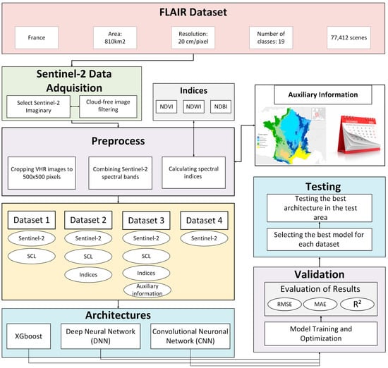
Figure 1.
End-to-end pipeline for fractional land cover mapping from Sentinel-2 data using deep learning.
In the preprocessing stage, very high-resolution (VHR) images (0.2 m per pixel) were cropped and co-registered to align with Sentinel-2 images. Based on the location of the FLAIR tiles, four different datasets are generated, each containing increasing levels of information. The first dataset includes Sentinel-2 pixel reflectance values together with the Scene Classification Layer (SCL, a per-pixel mask distinguishing surface types such as vegetation, water, clouds, and shadows) at 20 m resolution. The second dataset extends this by incorporating spectral indices derived from the Sentinel-2 bands, such as NDVI and other vegetation indices, alongside the reflectance and SCL data. The third dataset combines reflectance and SCL information with auxiliary variables, including climatic data and the acquisition date of the imagery, to provide additional contextual information. Finally, the fourth dataset consists solely of Sentinel-2 reflectance values. Over these areas, the Sentinel-2 Scene Classification Layer (SCL) and spectral bands are clipped, and spectral indices are calculated. Auxiliary information, such as predominant climate and image acquisition month, is also incorporated.
In the modeling phase, three approaches are employed, ranging from simplest to most complex: XGBoost, deep neural networks (DNN), and convolutional neural networks (CNN). The models are trained and optimized, and their performance is evaluated using metrics such as Mean Absolute Error (MAE), Root Mean Squared Error (RMSE), and the Coefficient of Determination (R2). A two-level validation scheme is applied, considering both the Sentinel-2 pixel level and the VHR scene level (aggregates of 5 × 5 Sentinel-2 pixels). Model performances are assessed using both validation datasets (which are also used in training the neural networks) and independent testing datasets.
2.2. Study Area
The study was conducted in France, a country located in Western Europe, approximately between 42° and 51° N latitude and −5° and 8° E longitude, characterized by diverse geography including plains, plateaus, and mountain ranges such as the Alps and the Pyrenees. With a total area of about 643,801 km2, France has a population of approximately 67 million inhabitants, mainly concentrated in urban areas such as Paris, Lyon, and Marseille, while rural regions exhibit significantly lower population densities. The climate varies across regions, with oceanic conditions in the northwest, Mediterranean in the southeast, continental in the northeast, and mountainous in the Alps and Pyrenees, resulting in notable differences in temperature and precipitation throughout the country. This geographic and climatic diversity directly influences land use, which includes forests, agricultural areas, and urban settlements.
Dataset Employed
The FLAIR-one dataset, developed by the French National Institute of Geographic and Forest Information (IGN), is designed to address semantic segmentation of aerial imagery and domain adaptation challenges in land cover mapping [11]. It covers approximately 810 km2 of metropolitan French territory, divided into 54 spatial domains that represent a wide variety of landscapes and climatic conditions, including urban, rural, agricultural, forest, and coastal areas. Each domain corresponds to a French administrative département.
The dataset contains 951 areas with a total of 77,412 aerial images acquired at a 0.2 m spatial resolution. Each image has 512 × 512 pixels, equivalent to approximately 1.05 ha. This approach provides a wide variety of representative examples for training and evaluating segmentation models. The data were collected in several acquisition campaigns between 2018 and 2021, specifically on 17 and 19 April and 16 September 2018; 1, 29 June, 4, 5, 10, 16, 25 July, 3, 14, 16, 23, 31 August, and 2 September, 11 October 2019; 25 June 2020; and 9 July 2021. The dataset is divided into three parts: 70% of the domains (38 domains) are allocated for training, while 15% (8 domains) are used for validation, and the other 15% (8 domains) for testing. This partition ensures independent assessment during model validation and testing analyses, as shown in Figure 2.
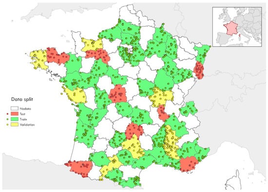
Figure 2.
Map showing the administrative departments of France as spatial units, with points inside each department representing locations where high-resolution images were acquired. These departments serve as the spatial domains for the analysis.
The labeling of FLAIR was carried out through manual photointerpretation by experts. This resulted in the creation of semantic masks (MSK) that assign a class to each pixel in the image. The original dataset contains 19 land cover classes, ranging from urban areas to natural and agricultural zones, among others.
Figure 3 illustrates the percentage distribution of classes across the dataset’s training, validation, and test sets. As can be seen, the last seven classes have a much lower distribution than the rest. Therefore, in this study, these will be merged into a combined class called “Other”. This reduced scheme, with 13 classes, aims to balance precision and simplicity, facilitating the implementation of classification models.
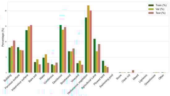
Figure 3.
Percentage distribution of land cover classes across training, validation, and test datasets.
2.3. Data Preprocessing
Sentinel-2 Imagery
The Sentinel-2 mission of the Copernicus Programme provides multispectral optical imagery with a spatial resolution of ≥10 m and a revisit frequency of ~5 days, making it a key source for studies such as this one. The Sentinel-2 Level-2A images used in this study are atmospherically corrected products, derived from Level-1C data through surface reflectance processing. These data are distributed free of charge by the European Space Agency (ESA) via platforms such as the Copernicus Dataspace Ecosystem, facilitating their use in scientific research and environmental management applications.
To enhance model training and ensure temporal consistency between data sources, the selected Sentinel-2 images cover a ±15-day window around the acquisition dates of the FLAIR very high-resolution (VHR) images. This approach minimizes discrepancies between data sources caused by the different acquisition times and eventual phenological or atmospheric variations. Moreover, this criterion allows for the inclusion of multiple Sentinel-2 images for a single reference date, thereby increasing the chances of cloud-free observations.
The Sentinel-2 Scene Classification Layer (SCL) is used to exclude observations contaminated by atmospheric effects or with the presence of clouds or cloud shadows, as indicated in Table 1. For the models, this index was encoded using the value of its corresponding code.

Table 1.
SCL Filter.
Sentinel-2 provides spectral information across 12 bands, ranging from the visible spectrum (RGB: red, green, and blue) to the shortwave infrared (SWIR), including the near-infrared (NIR) and several red-edge bands. In this study, all 12 Sentinel-2 bands are used, enabling a highly detailed characterization of the spectral signature of different land cover types [16].
In addition to the spectral bands, several spectral indices were used to generate the training datasets, in order to assess their contribution to land use classification [16]. Spectral indices are algebraic operations applied to the Sentinel-2 image bands, designed to enhance the discrimination between different land cover types.
The indices calculated for the database include the Normalized Difference Vegetation Index (NDVI), the Normalized Difference Water Index (NDWI), and the Normalized Difference Built-up Index (NDBI).
NDVI is used to assess active vegetation, where values greater than 0.5 are typically associated with dense vegetation, while values below 0.2 are indicative of bare soil or urban areas [38]. This index plays a significant role in crop monitoring and vegetation dynamics analysis [39].
The NDWI highlights the presence of surface water, with positive values typically associated with water bodies and negative values indicating dry soils or vegetation [40]. This index allows for the analysis of water bodies and their temporal dynamics [39].
Finally, NDBI facilitates the detection of built-up areas by exploiting the high reflectance of constructed surfaces in the SWIR1 band, distinguishing them from vegetation and natural soils [41]. This proves useful in urban expansion studies and land use classification [39].
2.4. Auxiliary Information
In addition to the spectral information provided by Sentinel-2 bands and vegetation indices, variables at a different scale, such as climate and data acquisition time, have been included. The climate, or even the seasonality within the same climate, can affect satellite image classification in several ways. Seasons impact the appearance of vegetation and soil, as plant phenology varies with temperature and precipitation in the course of the year. This can lead to differences in classifications performed at different times of the year, requiring adjustments or strategies like combining multiple dates to improve result consistency. Meanwhile, different climates can affect the greater or lesser presence of certain classes. Figure 4 shows the seven main climate types across the scenes, based on the FLAIR climate classification [42]. The “altered Mediterranean” climate was renamed into “Mediterranean”. The climates of France were categorized as: mountainous, oceanic, altered oceanic, degraded oceanic, Mediterranean, semi-continental, and southwestern basin, and for the models, these climates were encoded numerically from 0 to 7 in the order listed above.
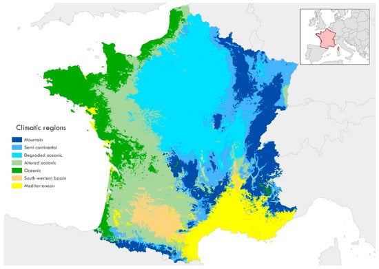
Figure 4.
Map illustrating the distinct climatic regions present in France, including Mountain, Semi-continental, Degraded oceanic, Altered oceanic, Oceanic, South-western basin, and Mediterranean.
Given the marked seasonal variations in land cover—e.g., agricultural cycles, vegetation phenology, and changes in water bodies—the month of image acquisition has been incorporated as an additional variable to improve the accuracy of satellite classification [43]. This temporal information allows for better capturing the land surface dynamics, such as crop growth [44,45], leaf senescence in deciduous forests [46,47], and seasonal fluctuations in water bodies [48], thereby reducing errors stemming from interpreting these changes as permanent land-use transformations.
2.5. Reduction of the VHR Image Size
The Sentinel-2 bands used in this study have a spatial resolution of 20 m and were kept in their original format. Each FLAIR very high-resolution (VHR) scene, measuring 512 × 512 pixels at 0.2 m per pixel (covering 102.4 × 102.4 m), is co-registered with Sentinel-2, meaning that the center of the scene aligns with the center of a Sentinel-2 pixel. To match precisely a 5 × 5 pixel block of Sentinel-2 (covering 100 × 100 m), a small margin of 1.2 m per side (6 × 512 pixels) was clipped from the VHR images, as shown in Figure 5.
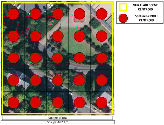
Figure 5.
Preprocessing of VHR Images from FLAIR.
2.6. Datasets Employed
The study evaluates four distinct datasets, each composed of different combinations of input variables (Table 2). This approach allows for understanding the contribution of each set of variables on model performance.
Table 2.
Combination of Elements from Each Dataset.
2.7. Architectures
In this study, diverse machine learning model architectures will be evaluated.
2.7.1. Extreme Gradient Boosting (XGBoost)
XGBoost is a machine learning algorithm based on decision trees that uses “boosting”, an approach to improve model accuracy [49]. Unlike traditional approaches that train trees independently, XGBoost builds trees sequentially, with each one correcting the errors made by previous trees. This iterative process efficiently optimizes the model, producing highly accurate results even with complex data. XGBoost is particularly powerful for classification and regression tasks due to its ability to handle non-linear relationships between features and its robustness against issues like overfitting. XGBoost has been successfully used in various studies focused on satellite image classification and land cover analysis, which supports its suitability for these types of applications [50,51,52]. The model was configured with a maximum tree depth of 10, learning rate (eta) of 0.1, subsample ratio of 0.8, column sample by tree of 0.8, and the number of trees (estimators) set to 500. Figure 6 illustrates the XGBoost model used where n is 500.
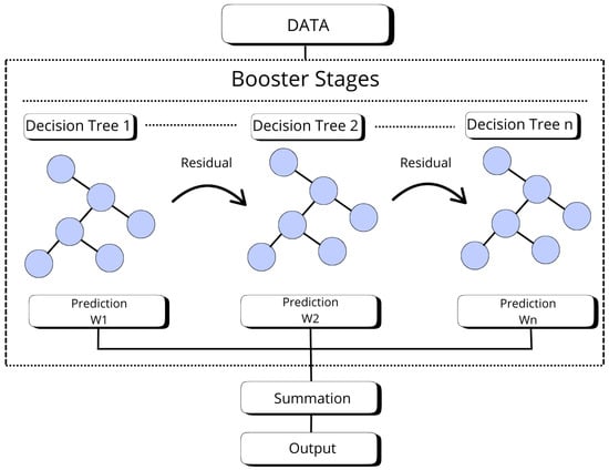
Figure 6.
XGBoost reference architecture.
2.7.2. Deep Neural Networks (DNNs)
Deep neural networks (DNNs) are machine learning models composed of multiple hidden layers between the input and output, enabling them to learn hierarchical and non-linear representations of data. Compared to traditional neural networks, DNNs are capable of handling large datasets and autonomously extracting complex patterns [53]. They are highly versatile and have been successfully applied to tasks such as classification, regression, and time series analysis [54]. In particular, DNNs are well-suited for problems involving complex, non-linear relationships between input features, such as the analysis of spectral data from satellite images [50,55]. Their effectiveness improves with larger datasets, allowing for enhanced prediction accuracy. Figure 7 illustrates the base DNN architecture employed in this study.
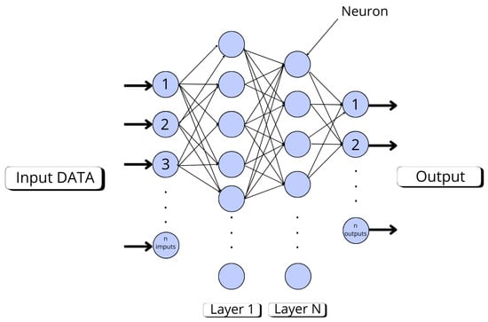
Figure 7.
Reference Architecture (Base DNN).
To assess the impact of model complexity, three DNN architectures with varying depths were tested:
Compact Architecture (DNN1)
This model features a simple architecture with three hidden layers of 128, 64, and 32 neurons, respectively, all activated with the ReLU function. Dropout layers have been incorporated after the first two hidden layers with a rate of 30% to mitigate overfitting, which helps improve model generalization. The output layer uses linear activation for regression. It was compiled with the Adam optimizer and the Mean Squared Error (MSE) loss function, which is suitable for regression tasks.
Intermediate Architecture (DNN2)
In this case, the model has the same Dropout structure but higher number of layers and neurons. It starts with 128 neurons in the first layer, followed by 256, 128, and 64 neurons in the last hidden layers. As with the previous model, the Adam optimizer and MSE loss are used.
Highly Dense Architecture (DNN3)
This model is the most complex and dense of the three, designed to capture more sophisticated patterns in the data. It starts with 512 neurons in the first layer and maintains a high number of neurons in the subsequent layers (512, 256, 256, 128, 128, 64, 64, and 32), allowing it to model highly complex non-linear relationships. The great depth and high number of parameters can give the model greater predictive capacity, but also make it more susceptible to overfitting and higher computational demands. ReLU activation is maintained in the hidden layers and linear in the output, along with the MSE loss function and the Adam optimizer.
2.7.3. Convolutional Neural Networks (CNNs)
CNNs are a type of deep neural network widely used for image processing and visual data analysis tasks. Their architecture is designed to recognize spatial and hierarchical patterns in data through convolutional layers that apply filters to extract important features, such as edges, textures, and shapes. These networks are especially effective in classification, segmentation, and object recognition tasks, as they can learn representations at different scales without manual intervention [56].
In the context of remote sensing, CNNs are ideal for analyzing satellite images or remote sensing data, as they can identify complex patterns in multispectral data and classify different land cover classes with high accuracy [57,58]. Their ability to generalize patterns from spatial data makes them a relevant tool in land use classification with Sentinel-2 images.
The implemented architecture consists of two convolutional layers with ReLU activation functions, configured with 32 and 64 filters respectively and a kernel size of 3 × 3 with 1 padding, which allows preserving the spatial resolution of the input. These layers are designed to capture hierarchical and local representations of spatial features. Subsequently, a flattening operation is applied, followed by a fully connected layer of 128 units and an output layer corresponding to the number of target classes. No activation is applied in the output layer, as the BCEWithLogitsLoss function is used, which combines sigmoid activation with binary cross-entropy, making it suitable for multi-label classification tasks. Figure 8 illustrates the base CNN architecture used in this study.
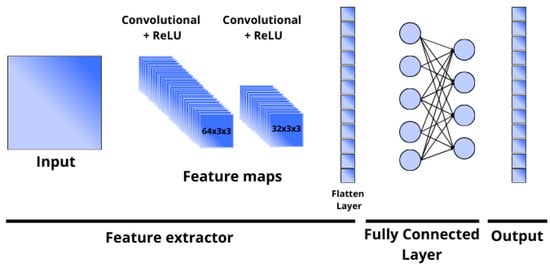
Figure 8.
CNN reference architecture.
2.8. Validation and Metrics
To ensure the accuracy and reliability of the estimated land cover fractions, the validation process is carried out at two levels: pixel-level validation and scene-level validation. These complementary approaches allow for a comprehensive evaluation of model performance.
Since the model outputs are constrained to range from 0 to 100 and the predicted fractions for all land cover classes within each pixel always sum to 100, the resulting RMSE and MAE values are directly interpretable as percentage errors. This also applies to scene-level validation, where aggregated predictions retain this percentage-based interpretation.
2.8.1. Pixel-Level Validation
At the pixel level, the estimated land cover fractions for each class are compared with the reference fractions obtained from the FLAIR dataset. This approach allows evaluating the model’s ability to accurately predict the fraction of each class within individual Sentinel-2 pixels. To this end, some of the metrics proposed by [59] for validating machine learning models were selected.
- Root Mean Squared Error (RMSE): A metric used to evaluate the accuracy of a regression model. It is calculated as the square root of the mean squared error (MSE), which allows interpreting the error in the same units as the target variable.
- Mean Absolute Error (MAE): Calculates the average absolute difference between the estimated and actual fractions, providing an intuitive measure of the error.
- Coefficient of Determination (R2): Evaluates the proportion of variance in the actual fractions that is explained by the model’s predictions. Values close to 1 indicate a strong correlation.where is the observed fractional land cover derived from the FLAIR dataset and the estimated fractional land cover in each Sentinel-2 pixel . refers to the number of Sentinel-2 pixels.
2.8.2. Scene-Level Validation
A complete scene covers a 100 × 100 m surface and contains 25 Sentinel-2 20 m pixels. The same error metrics mentioned above (MAE, RMSE, R2) are used. In this case the definitions of and are modified: refers to a scene, to the number of scenes (), and
where refers in this case to a Sentinel-2 pixel and to the number of Sentinel-2 pixels in each FLAIRS scene (), which cover an area of 10,000 m2.
2.9. Class-Level Model Evaluation Against the Test Set
To achieve a more detailed evaluation of model performance, global errors are complemented with a class-level analysis using the test set. This approach is particularly relevant for determining the model’s individual accuracy within each land cover category, offering a better characterization of the model’s performance on imbalanced classes or those with similar spectral characteristics. The same statistical metrics from previous sections are applied but calculated specifically for each class. This allows for the identification of the best and worst performing categories.
2.10. Comparison with Copernicus Global Land Cover
To assess the performance of our model, we conducted a comparison with the Copernicus Global Land Cover (CGLS-LC100, fractional) product. For this purpose, we built a homogeneous dataset integrating three sources of information: the manually labeled ground truth (GT), the predictions generated by our model from very high-resolution aerial imagery, and the Copernicus fractional cover estimates. Since the class definitions across the two datasets did not fully align, we harmonized the categories to enable direct comparison. Specifically, tree cover classes (Coniferous, Deciduous, Ligneous) were grouped under Tree cover; Brushwood was mapped to Shrubland; Agricultural land, Plowed land, and Vineyard were aggregated into Cropland; Herbaceous vegetation was retained as an independent class; Bare soil and Pervious surface were integrated into Bare/sparse vegetation; Water was directly aligned with the Water category; and urban/artificial surfaces (Building, Impervious surface) were grouped under Built-up. After this reaggregation, all class fractions were normalized so that each image summed to 100%. This harmonization provided a consistent framework to evaluate agreement between our predictions and the Copernicus reference product, allowing us to identify systematic differences across land cover types and to better understand the strengths and limitations of our approach relative to a widely used continental-scale dataset.
3. Results
3.1. Validation
Table 3 and Table 4 show the model performance results evaluated against the validation dataset. When jointly analyzing the pixel-level and scene-level metrics for DNN1, DNN2, DNN3, XGBoost, and CNN, a clear pattern emerges: the mean errors (MSE, MAE, and RMSE) are higher in pixel-level validation and decrease significantly when pixels are aggregated into 100 × 100 m units (scene level). Conversely, the coefficient of determination (R2) increases at the scene level, reflecting a better capture of aggregated spatial variability.
Table 3.
Dataset 1 (Sentinel-2 + SCL) Pixel-Level Validation Metrics.
Table 4.
Dataset 1 (Sentinel-2 + SCL) Scene-Level Validation Metrics.
At both levels, DNN2 and DNN3 yield the best results in terms of MSE and MAE, closely followed by XGBoost. DNN1, being the simplest architecture, shows slightly inferior performance. The CNN, on the other hand, exhibits the highest average error values in both tables, but surprisingly boasts the highest R2 at both pixel and scene levels. This indicates that despite its larger absolute bias, it better explains the overall variance.
The inclusion of spectral indices did not improve the performance of the deep neural networks (DNNs); in fact, their metrics remained largely unchanged (Table 5 and Table 6). This is likely because the indices introduced redundant information derived from the original bands, increasing the dimensionality without adding new value. Similarly, CNNs and XGBoost were barely affected by the addition of these indices. In the case of CNNs, the architecture already extracts relevant spatial and spectral patterns directly from the input bands. XGBoost, on the other hand, is capable of automatically disregarding non-informative variables, such as spectral indices that do not contribute additional information.
Table 5.
Dataset 2 (Sentinel-2 + Indices + SCL) pixel level validation metrics.
Table 6.
Dataset 2 (Sentinel-2 + Indices + SCL) scene level validation metrics.
While none of the models showed improvements at the pixel level, XGBoost did achieve a noticeable enhancement at the scene level, reaching a mean absolute error (MAE) of 1.47. This improvement is likely due to its feature selection mechanism, which helps mitigate the impact of redundant or irrelevant inputs.
The inclusion of auxiliary information, such as temporal variables or climate data, does contribute to improved performance, particularly at the scene level (Table 7 and Table 8). While DNN2 achieves its best pixel-level MAE to date with this input combination (5.05), the most notable gains are observed at the scene level, where the results outperform those obtained with other input configurations.
Table 7.
Dataset 3 (Sentinel-2 + Indices + SCL + Auxiliary information) pixel level validation metrics.
Table 8.
Dataset 3 (Sentinel-2 + Indices + SCL + Auxiliary information) scene level validation metrics.
In this specific context, DNN2 achieves the best results at both pixel and scene levels, outperforming both XGBoost and CNN (Table 9 and Table 10). This suggests that when the input is limited to the essential Sentinel-2 bands, DNN2 yields the lowest MAE and MSE, though not the highest R2.
Table 9.
Dataset 4 (Sentinel-2) pixel level validation metrics.
Table 10.
Dataset 4 (Sentinel-2) scene level validation metrics.
3.2. Dataset and Model Selection
The models that achieved the best results in terms of MAE and RMSE against the validation set for each dataset were then evaluated on the independent test set (unseen during training), yielding the following results at both global and class levels.
3.2.1. Pixel-Level
Despite the low coefficients of determination (R2) obtained across the four datasets—with values between 0.39 and 0.41—the other metrics are reasonably good given the problem’s context (Table 11). The Mean Absolute Error (MAE) ranges from 5.42 to 5.86.
Table 11.
Metrics of top-performing architectures for each dataset at pixel level.
The class-specific results reveal considerable variability in model performance (Figure 9). This figure includes the most representative and prevalent classes in the dataset, providing insight into how the model handles the most common land cover types. Generally, classes with lower spectral variability or greater homogeneity—such as Bare soil and Vineyard—exhibit the best performance metrics, with low MAE values (2.89 and 2.35, respectively) and high R2 coefficients (0.53 for both), indicating high precision and strong correspondence with ground truth. Water and Plowed land also demonstrate solid performance, with R2 values of 0.51 and 0.48, respectively, and low errors (MAE of 4.61 and 2.97), suggesting the model’s good capability in predicting these categories. Conversely, more heterogeneous classes or those with greater spectral similarity to others—such as Herbaceous vegetation, Deciduous, Agricultural land, Impervious surface, and Pervious surface—present the highest errors. Notably, Herbaceous vegetation has the lowest R2 (0.23) and the highest MAE (17.59), while Deciduous and Agricultural land also show elevated MAE values (16.24 and 10.83, respectively), reflecting the model’s difficulty in capturing their internal variability and effectively distinguishing them from spectrally similar classes.
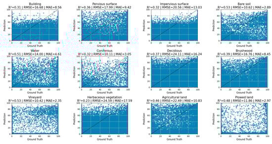
Figure 9.
Scatter plots by class—Pixel-level fractional cover predictions vs. ground truth.
3.2.2. Scene-Level
The scene-level results at 100-m resolution show a clear improvement over those obtained at 20 m, which is consistent with what was observed in the validation set. In this case, the coefficients of determination (R2) range between 0.59 and 0.67 (Table 12). Additionally, MAE is significantly reduced, settling around 2.36–2.94. The RMSE also decreases notably, with values between 4.94 and 6.09.
Table 12.
Metrics of the Best Architectures for Each Dataset at Scene Level in the Test Set.
The class-specific results from this analysis, conducted at the scene level (100 m resolution), demonstrate notable improvements in model performance across various categories compared to the previous pixel-level (20 m resolution) assessment (Figure 10). As in the previous analysis, Figure 10 includes only the most representative and frequent classes in the dataset, ensuring a meaningful comparison across dominant land cover types. The enhanced performance observed is largely attributable to the aggregation of information at a coarser scale, which reduces pixel-level noise and better captures the dominant land cover signals. Classes with inherently clearer spectral signatures or greater homogeneity—such as Bare soil, Water, and Vineyard—now exhibit excellent metrics, with R2 values of 0.81 in all three cases and remarkably low MAE values (2.18, 3.02, and 1.67, respectively), indicating very strong agreement with ground truth. Building also shows a significant improvement, achieving an R2 of 0.71 and an MAE of 4.52. Furthermore, classes that previously presented challenges at the pixel level, like Impervious surface, Plowed land, and Agricultural land, now demonstrate solid performance with R2 values of 0.73, 0.72, and 0.74, and correspondingly lower errors (MAE of 6.06, 2.29, and 7.40). While classes such as Deciduous, Brushwood, Pervious surface, and Coniferous show good R2 values (ranging from 0.63 to 0.75), their MAE values remain comparatively higher, suggesting that some internal variability or spectral confusion persists even at the scene level. Herbaceous vegetation, although notably improved from its pixel-level performance, still presents the lowest R2 (0.58) and the highest MAE (8.90) among all classes, indicating it remains the most challenging category for precise prediction—likely due to its high heterogeneity and temporal variability, which may persist even after spatial aggregation.
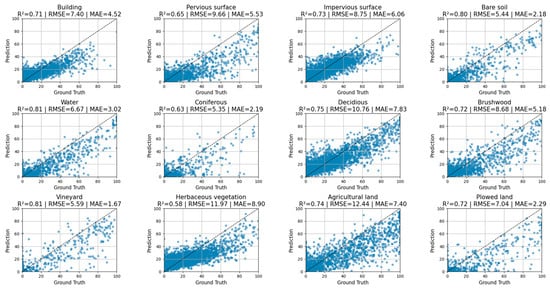
Figure 10.
Scatter plots by class—Scene-level fractional cover predictions vs. ground truth.
3.3. Comparation with CGLS-LC100
Figure 11 shows both visual and quantitative evaluations of land cover classification performance for two models: the model developed in this study (“Our Pred”) and the Copernicus model (CGLS-LC100). The assessment was conducted across three urban and peri-urban scenarios, using the high-resolution FLAIR-GT dataset as the ground truth.
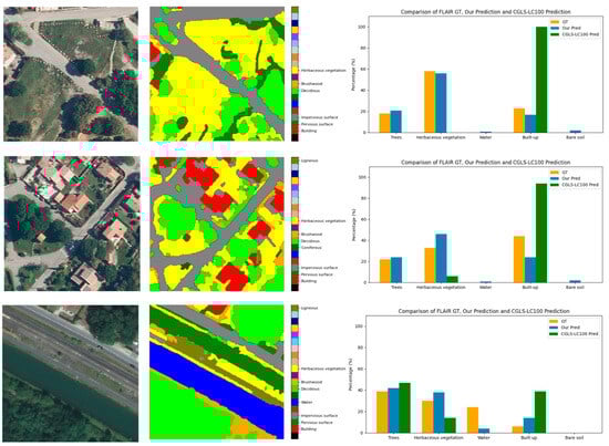
Figure 11.
Examples of 100 × 100 m scenes showing ground-truth fractional cover, our model predictions, and CGLS-LC100 predictions.
Across all scenarios, the “Our Pred” model exhibited strong agreement with the FLAIR-GT reference. This is reflected in the visual representation of land cover classes and the corresponding area proportions shown in the histograms. The model produced well-balanced predictions across categories such as trees, herbaceous vegetation, water, built-up areas, and bare soil.
In contrast, the Copernicus (CGLS-LC100) model showed notable biases. In the first two scenarios, it consistently overestimated built-up areas, suggesting potential confusion between constructed structures and other land cover types such as vegetation or bare soil. In the third scenario, this trend reversed, with a significant underestimation of built-up areas, highlighting inconsistencies in local-level predictions.
4. Discussion
Although continuous or fractional mapping approaches have traditionally received less attention than their discrete approaches, recent studies and operational products have begun to highlight their advantages and feasibility. One notable example is the work by Masiliūnas et al. [37], who employed Landsat 8 imagery and the Random Forest (RF) algorithm to estimate fractional cover for seven land cover classes. In a more advanced implementation, Copernicus Global Land Cover delivers global fractional cover for ten classes at a spatial resolution of 100 m, explicitly adopting a continuous perspective [21].
Compared to studies like that of Masiliūnas et al. [37], which relied on conventional architectures such as RF, the present study explores more advanced models. These include XGBoost—a direct improvement of RF—as well as deep neural networks (DNNs) with varying depths and convolutional neural networks (CNNs). The results demonstrate a clear performance improvement: while Masiliūnas et al. [37] reported a mean absolute error (MAE) of 7.9 at 100 m resolution for seven classes, our approach achieved a substantially lower MAE of 2.36 despite working with a much broader set of 13 classes. These findings underscore the potential of combining finer input data, broader class diversity, and more advanced modeling architectures to improve fractional land cover estimation. Future work could directly compare both approaches under standardized dataset and resolution settings to isolate the effect of model complexity and input richness.
Another key advantage—though also a challenge—is the number of land cover classes considered. While the aforementioned studies and products typically work with fewer than 10 classes, this study addresses a broader thematic diversity with 13 classes. This increased thematic richness enables a more detailed characterization of the landscape.
Our results at the pixel level (20 m resolution) yielded MAEs around 5–6, which is reasonable for heterogeneous cover types. Nonetheless, the low coefficients of determination (mean R2 = 0.41) at this scale suggest that the variance explained at the individual pixel level is limited. This indicates that, although the model captures the overall trend, predicting fractions at the pixel level remains challenging in complex environments, particularly for classes with high variability. Classes such as “Herbaceous vegetation,” “Agricultural land,” and “Deciduous” showed the highest pixel-level errors, with MAEs up to 17.59 and RMSEs exceeding 24. In contrast, classes like “Water,” “Bare soil,” “Plowed land,” and “Vineyard” had lower MAEs and better R2 values. This pattern is also reflected in the scatter plots, where a wide dispersion of predicted versus reference values is observed at the pixel level.
The notable improvement in performance metrics when validating the models at the scene level (100 m resolution) underscores the suitability of the approach for regional-scale analyses. At 100 m, the mean R2 increased significantly to 0.67, while the MAE decreased to values between 2.36 and 2.94—indicating very low average errors. The scatter plots at this coarser resolution display a much tighter distribution around the 1:1 line, with reduced dispersion and fewer outliers, highlighting the improved consistency of predictions after spatial aggregation. At the class level, classes such as “Water,” “Vineyard,” “Bare soil,” and “Plowed land” achieved high R2 values (0.81, 0.81, 0.80, and 0.72, respectively), with very low MAEs, even approaching or falling below 2 in the case of “Bare soil,” “Water,” “Vineyard,” “Plowed land,” and “Coniferous.” This improved performance at coarser spatial resolution reflects, as expected, how errors tend to cancel each other as the size of the spatial unit of analysis increases, and supports the robustness of the model for regional applications. These findings align with previous relevant studies, such as Marceau et al. [60] and Buchhorn et al. [21].
The study evaluated the performance of different machine learning architectures—DNNs, CNNs, and XGBoost—using four distinct datasets to assess the contribution of various input variables. Overall, results were relatively consistent across models. The intermediate DNN2 architecture consistently achieved the best results at the pixel level (20 m), while XGBoost outperformed all other models at the scene level (100 m) on the independent test set. When spectral indices were included (Dataset 2), DNNs underperformed—likely due to increased dimensionality and redundancy, which added noise, as noted by Romero et al. [61]. In contrast, XGBoost and CNNs were less affected. XGBoost efficiently manages redundancy by discarding irrelevant features or assigning them low weights [49], and CNNs are designed to extract relevant patterns directly from the original spectral bands [62].
Dataset 3, which included auxiliary variables such as temporal and climate data, produced general improvements across all models—particularly at the scene level. This highlights the value of contextual information and suggests that such variables may enhance model performance more effectively than spectral indices alone. These results emphasize the importance of tailoring both model architecture and input features to the specific task and scale of analysis.
The comparison between “Our Pred” and Copernicus CGLS-LC100 highlights that while the Copernicus model is suitable for regional-scale analyses, it shows inconsistencies at the local scale, such as over- or underestimating built-up areas due to mixed land cover signals and limited spatial resolution. In contrast, the “Our Pred” model demonstrates higher accuracy and balanced classification, indicating that high-resolution, tailored approaches are better suited for detailed urban and peri-urban land cover mapping. These results underscore the value of localized model training and high-resolution reference data for improving predictive reliability and supporting planning and environmental monitoring in complex landscapes.
The use of fractional land cover maps provides a more detailed representation of landscape heterogeneity compared to traditional discrete maps. This approach enables a wide range of environmental applications: carbon stock estimation benefits from weighting the different pools according to the proportion of each class within a pixel, improving accuracy compared to assuming full occupation by a single class; hydrological models can incorporate actual proportions of vegetation, bare soil, and impervious surfaces to refine calculations of runoff, infiltration, and evapotranspiration; and biodiversity and habitat assessments are enhanced by capturing habitat mosaics and sub-pixel heterogeneity, supporting more realistic species distribution and habitat suitability models. Despite the advances presented, the proposed approach has limitations. Although a pixel-level MAE of around 5 is reasonable, the low R2 at this scale suggests limited explanatory power for individual pixels. Thus, while the model captures general trends, pixel-level prediction remains challenging in complex environments. However, the significant improvement in scene-level metrics (100 m) validates the applicability of our model for regional-scale analysis.
A key limitation compared to global products like Copernicus CGLS-LC100, or even broader studies such as Masiliūnas et al. [37], is the geographical scope. Our current focus is regional—specifically in France—using the FLAIR dataset. While this allows for more precise calibration and may explain the better MAE scores, broader applicability remains to be tested. Nonetheless, model transferability is feasible. Studies like as demonstrated in studies like Safarov et al. [63] and Sierra et al. [14] demonstrate that CNNs can be used to generate labels in new regions, reducing the need for manual annotation and enabling expansion of the training dataset.
Future research could explore incorporating the temporal dimension in Sentinel-2 time series to better capture phenological dynamics, thereby improving the classification of seasonally varying classes. Additionally, hybrid architectures that combine the feature-handling capabilities of XGBoost with the spatial pattern extraction power of CNNs may further enhance model robustness. Finally, testing across a wider range of environments will be crucial for evaluating model transferability and potential for global applications.
5. Conclusions
This study presents a methodology for mapping fractional land cover using Sentinel-2 imagery and artificial intelligence models. Unlike traditional discrete classification approaches, the proposed method offers a more realistic depiction of landscape heterogeneity, particularly in pixels composed of mixed land cover types.
A key contribution of this research lies in addressing a gap in the current state of the art: most previous studies on fractional land cover have focused on global scales with a limited number of broad classes. In contrast, this work broadens the thematic scope by estimating fractional cover for up to 13 land cover classes. The methodology is developed and validated using the FLAIR dataset, which covers 810 km2 of French territory at 0.2 m resolution and includes expert-annotated land cover data. Four dataset variants were tested, combining Sentinel-2 spectral bands, scene classification (SCL), derived vegetation indices, and auxiliary variables such as climate zone and image acquisition date.
France was chosen as the study area due to its wide range of climates and land cover types, including oceanic, Mediterranean, continental, and mountainous regions, ensuring that the methodology is exposed to diverse environmental conditions and better prepared for adaptation to other regions. Although developed and validated using French data, the methodology is transferable to other areas with similar Sentinel-2 coverage and heterogeneous landscapes. For example, it could be applied to temperate European countries such as Germany, Poland, or Spain, as well as to parts of North America like the northeastern United States or southern Canada. In these regions, the approach could be used directly, but fine-tuning with local training data would likely improve accuracy by adapting the models to region-specific land cover patterns and climate variability.
Three modeling strategies were compared—XGBoost, deep neural networks (DNNs), and convolutional neural networks (CNNs)—to evaluate the impact of model complexity and input configuration on estimation accuracy. DNN2 and XGBoost showed the best results in terms of RMSE and MAE at the pixel (13.83 and 5.42) and scene level (4.94 and 2.36), respectively. CNNs, on the other hand, achieved the best coefficient of determination (R2), highlighting the potential of deep learning architectures to capture more complex spatial patterns, even if they do not always outperform in absolute error metrics.
Although results at the 20 m pixel level are promising, scatterplots reveal high variability in pixel-wise predictions. These findings suggest that aggregating predictions at coarser resolutions—such as 100 m—may yield more robust and consistent outputs, aligning better with current global-scale studies and reducing local noise. Finally, fractional land cover mapping represents a major step forward compared to discrete approaches, particularly in environmental applications such as carbon stock estimation. By avoiding the assumption that each pixel is fully occupied by a single class, fractional estimates offer a more nuanced view of land cover, especially in transitional or heterogeneous areas. Thanks to the use of Sentinel-2 data and relatively simple AI architectures, this approach remains scalable and cost-effective, with strong potential for frequent updates. The promising performance of deep learning models reinforces their value as tools for accurate and timely land monitoring.
Author Contributions
Conceptualization, S.S., R.R. and A.C.; methodology, S.S. and R.R.; software, S.S.; validation, S.S. and M.P.; formal analysis, S.S. and R.R.; investigation, S.S.; resources, S.S. and L.Q.; data curation, S.S. and L.Q.; writing—original draft preparation, S.S.; writing—review and editing, R.R., A.C., M.P., L.Q.; supervision, R.R. and A.C.; project administration, A.C. All authors have read and agreed to the published version of the manuscript.
Funding
This research was supported by the industrial doctorate grant DIN2021-011907 funded by MICIU/AEI/https://doi.org/10.13039/501100011033 and DI37 funded by Universidad de Cantabria and project “Photonic Sensors for Sustainable Smart Cities PERFORMANCE” PID2022-137269OB-C22l(MICIU/AEI/https://doi.org/10.13039/501100011033andERDF/EU).
Data Availability Statement
The data supporting this study are based on the FLAIR dataset, which is a publicly available dataset at https://ignf.github.io/FLAIR/FLAIR1/flair_1.html (accessed on 12 December 2024).
Conflicts of Interest
The authors declare no conflicts of interest.
Abbreviations
The following abbreviations are used in this manuscript:
| DNN | Deep Neural Network |
| CNN | Convolutional Neural Network |
| RMSE | Root Mean Squared Error |
| MAE | Mean Absolute Error |
| R2 | Coefficient of Determination |
| LC | Land Cover |
| FLAIR | French Land cover from Aerospace ImageRy |
| VHR | Very High-Resolution |
| ESA | European Space Agency |
| SCL | Scene Classification Layer |
| RGB | Red, Green, and Blue |
| SWIR | Shortwave Infrared |
| NIR | Near-Infrared |
| NDVI | Normalized Difference Vegetation Index |
| NDWI | Normalized Difference Water Index |
| NDBI | Normalized Difference Built-up Index |
| MSE | Mean Squared Error |
References
- Lillesand, T.; Kiefer, R.W.; Chipman, J. Remote Sensing and Image Interpretation; John Wiley & Sons: Hoboken, NJ, USA, 2015; ISBN 111834328X. [Google Scholar]
- Yang, C.; Yu, Z.; Hao, Z.; Lin, Z.; Wang, H. Effects of Vegetation Cover on Hydrological Processes in a Large Region: Huaihe River Basin, China. J. Hydrol. Eng. 2013, 18, 1477–1483. [Google Scholar] [CrossRef]
- Bastin, J.-F.; Finegold, Y.; Garcia, C.; Mollicone, D.; Rezende, M.; Routh, D.; Zohner, C.M.; Crowther, T.W. The Global Tree Restoration Potential. Science 2019, 365, 76–79. [Google Scholar] [CrossRef]
- Foley, J.A.; DeFries, R.; Asner, G.P.; Barford, C.; Bonan, G.; Carpenter, S.R.; Chapin, F.S.; Coe, M.T.; Daily, G.C.; Gibbs, H.K. Global Consequences of Land Use. Science 2005, 309, 570–574. [Google Scholar] [CrossRef]
- Kõlli, R.; Kanal, A. The Management and Protection of Soil Cover: An Ecosystem Approach. For. Stud. 2010, 53, 25. [Google Scholar] [CrossRef]
- Montgomery, D.R. Soil Erosion and Agricultural Sustainability. Proc. Natl. Acad. Sci. USA 2007, 104, 13268–13272. [Google Scholar] [CrossRef] [PubMed]
- Tscharntke, T.; Klein, A.M.; Kruess, A.; Steffan-Dewenter, I.; Thies, C. Landscape Perspectives on Agricultural Intensification and Biodiversity–Ecosystem Service Management. Ecol. Lett. 2005, 8, 857–874. [Google Scholar] [CrossRef]
- Weiland, S.; Hickmann, T.; Lederer, M.; Marquardt, J.; Schwindenhammer, S. The 2030 Agenda for Sustainable Development: Transformative Change through the Sustainable Development Goals? Politics Gov. 2021, 9, 90–95. [Google Scholar] [CrossRef]
- Cover, C.L. Corine Land Cover; European Environment Agency: Copenhagen, Denmark, 2000. [Google Scholar]
- Büttner, G.; Feranec, J.; Jaffrain, G.; Mari, L.; Maucha, G.; Soukup, T. The CORINE Land Cover 2000 Project. EARSeL eProceedings 2004, 3, 331–346. [Google Scholar]
- Garioud, A.; Peillet, S.; Bookjans, E.; Giordano, S.; Wattrelos, B. FLAIR: French Land Cover from Aerospace ImageRy. arXiv 2022, arXiv:2305.14467v1. [Google Scholar]
- Garioud, A.; Peillet, S.; Bookjans, E.; Giordano, S.; Wattrelos, B. Flair# 1: Semantic Segmentation and Domain Adaptation Dataset. arXiv 2022, arXiv:2211.12979. [Google Scholar]
- Xia, J.; Yokoya, N.; Adriano, B.; Broni-Bediako, C. Openearthmap: A Benchmark Dataset for Global High-Resolution Land Cover Mapping. In Proceedings of the IEEE/CVF Winter Conference on Applications of Computer Vision, Waikoloa, HI, USA, 2–7 January 2023; pp. 6254–6264. [Google Scholar]
- Sierra, S.; Ramo, R.; Padilla, M.; Cobo, A. Optimizing Deep Neural Networks for High-Resolution Land Cover Classification through Data Augmentation. Environ. Monit. Assess. 2025, 197, 423. [Google Scholar] [CrossRef]
- Drusch, M.; Del Bello, U.; Carlier, S.; Colin, O.; Fernandez, V.; Gascon, F.; Hoersch, B.; Isola, C.; Laberinti, P.; Martimort, P. Sentinel-2: ESA’s Optical High-Resolution Mission for GMES Operational Services. Remote Sens. Environ. 2012, 120, 25–36. [Google Scholar] [CrossRef]
- Phiri, D.; Simwanda, M.; Salekin, S.; Nyirenda, V.R.; Murayama, Y.; Ranagalage, M. Sentinel-2 Data for Land Cover/Use Mapping: A Review. Remote Sens. 2020, 12, 2291. [Google Scholar] [CrossRef]
- Wang, Z.; Song, D.-X.; He, T.; Lu, J.; Wang, C.; Zhong, D. Developing Spatial and Temporal Continuous Fractional Vegetation Cover Based on Landsat and Sentinel-2 Data with a Deep Learning Approach. Remote Sens. 2023, 15, 2948. [Google Scholar] [CrossRef]
- Zikiou, N.; Rushmeier, H. Sentinel-2 Data Classification for Land Use Land Cover Mapping in Northern Algeria. In Proceedings of the Algorithms, Technologies, and Applications for Multispectral and Hyperspectral Imaging XXIX, Orlando, FL, USA, 30 April–5 May 2023; Volume 12519, pp. 147–161. [Google Scholar]
- Thierion, V.; Vincent, A.; Valero, S. Theia OSO Land Cover Map 2021; Zenodo: Geneva, Switzerland, 2022; Version 1. [Google Scholar] [CrossRef]
- S2GLC. Available online: https://s2glc.cbk.waw.pl/ (accessed on 20 May 2020).
- Buchhorn, M.; Smets, B.; Bertels, L.; De Roo, B.; Lesiv, M.; Tsendbazar, N.-E.; Herold, M.; Fritz, S. Copernicus Global Land Service: Land Cover 100 m: Collection 3: Epoch 2019: Globe. 2020. Available online: https://zenodo.org/record/3939050 (accessed on 2 October 2025).
- Tsendbazar, N.-E.; Tarko, A.; Li, L.; Herold, M.; Lesiv, M.; Fritz, S.; Maus, V. Copernicus Global Land Service: Land Cover 100m: Version 3 Globe 2015–2019: Validation Report; Zenodo: Geneva, Switzerland, 2021; CGLOPS1_VR_LC100m-V3.0_I1.10. [Google Scholar]
- Okeke, F.; Karnieli, A. Linear Mixture Model Approach for Selecting Fuzzy Exponent Value in Fuzzy C-Means Algorithm. Ecol. Inform. 2006, 1, 117–124. [Google Scholar] [CrossRef]
- Adams, J.B.; Sabol, D.E.; Kapos, V.; Almeida Filho, R.; Roberts, D.A.; Smith, M.O.; Gillespie, A.R. Classification of Multispectral Images Based on Fractions of Endmembers: Application to Land-Cover Change in the Brazilian Amazon. Remote Sens. Environ. 1995, 52, 137–154. [Google Scholar] [CrossRef]
- Foody, G.M. Approaches for the Production and Evaluation of Fuzzy Land Cover Classifications from Remotely-Sensed Data. Int. J. Remote Sens. 1996, 17, 1317–1340. [Google Scholar] [CrossRef]
- Walton, J.T. Subpixel Urban Land Cover Estimation. Photogramm. Eng. Remote Sens. 2008, 74, 1213–1222. [Google Scholar] [CrossRef]
- Hansen, M.C.; Egorov, A.; Roy, D.P.; Potapov, P.; Ju, J.; Turubanova, S.; Kommareddy, I.; Loveland, T.R. Continuous Fields of Land Cover for the Conterminous United States Using Landsat Data: First Results from the Web-Enabled Landsat Data (WELD) Project. Remote Sens. Lett. 2011, 2, 279–288. [Google Scholar] [CrossRef]
- Shankar, B.U.; Meher, S.K.; Ghosh, A. Wavelet-Fuzzy Hybridization: Feature-Extraction and Land-Cover Classification of Remote Sensing Images. Appl. Soft. Comput. 2011, 11, 2999–3011. [Google Scholar] [CrossRef]
- Gessner, U.; Machwitz, M.; Conrad, C.; Dech, S. Estimating the Fractional Cover of Growth Forms and Bare Surface in Savannas. A Multi-Resolution Approach Based on Regression Tree Ensembles. Remote Sens. Environ. 2013, 129, 90–102. [Google Scholar] [CrossRef]
- Okujeni, A.; Canters, F.; Cooper, S.D.; Degerickx, J.; Heiden, U.; Hostert, P.; Priem, F.; Roberts, D.A.; Somers, B.; van der Linden, S. Generalizing Machine Learning Regression Models Using Multi-Site Spectral Libraries for Mapping Vegetation-Impervious-Soil Fractions across Multiple Cities. Remote Sens. Environ. 2018, 216, 482–496. [Google Scholar] [CrossRef]
- Colditz, R.R. An Evaluation of Different Training Sample Allocation Schemes for Discrete and Continuous Land Cover Classification Using Decision Tree-Based Algorithms. Remote Sens. 2015, 7, 9655–9681. [Google Scholar] [CrossRef]
- Hansen, M.C.; DeFries, R.S.; Townshend, J.R.G.; Carroll, M.; Dimiceli, C.; Sohlberg, R.A. Global Percent Tree Cover at a Spatial Resolution of 500 Meters: First Results of the MODIS Vegetation Continuous Fields Algorithm. Earth Interact. 2003, 7, 1–15. [Google Scholar] [CrossRef]
- Townshend, J. Global Forest Cover Change (GFCC) Tree Cover Multi-Year Global 30 m V003; Processes Distributed Active Archive Center (DAAC): Sioux Falls, SD, USA, 2016; NASA EOSDIS Land. Data Set, GFCC30TC-003. [Google Scholar]
- Pekel, J.-F.; Cottam, A.; Gorelick, N.; Belward, A.S. High-Resolution Mapping of Global Surface Water and Its Long-Term Changes. Nature 2016, 540, 418–422. [Google Scholar] [CrossRef] [PubMed]
- Corbane, C.; Pesaresi, M.; Kemper, T.; Politis, P.; Florczyk, A.J.; Syrris, V.; Melchiorri, M.; Sabo, F.; Soille, P. Automated Global Delineation of Human Settlements from 40 Years of Landsat Satellite Data Archives. Big Earth Data 2019, 3, 140–169. [Google Scholar] [CrossRef]
- Gao, J.; O’Neill, B.C. Mapping Global Urban Land for the 21st Century with Data-Driven Simulations and Shared Socioeconomic Pathways. Nat. Commun. 2020, 11, 2302. [Google Scholar] [CrossRef] [PubMed]
- Masiliūnas, D.; Tsendbazar, N.-E.; Herold, M.; Lesiv, M.; Buchhorn, M.; Verbesselt, J. Global Land Characterisation Using Land Cover Fractions at 100 m Resolution. Remote Sens. Environ. 2021, 259, 112409. [Google Scholar] [CrossRef]
- Jw, R. Monitoring Vegetation Systems in the Great Plains with ERTS. In Proceedings of the Third NASA Earth Resources Technology Satellite Symposium, Washington, DC, USA, 10–14 December 1973; Volume 1, pp. 309–317. [Google Scholar]
- Zheng, Y.; Tang, L.; Wang, H. An Improved Approach for Monitoring Urban Built-up Areas by Combining NPP-VIIRS Nighttime Light, NDVI, NDWI, and NDBI. J. Clean. Prod. 2021, 328, 129488. [Google Scholar] [CrossRef]
- McFeeters, S.K. The Use of the Normalized Difference Water Index (NDWI) in the Delineation of Open Water Features. Int. J. Remote Sens. 1996, 17, 1425–1432. [Google Scholar] [CrossRef]
- Zha, Y.; Gao, J.; Ni, S. Use of Normalized Difference Built-up Index in Automatically Mapping Urban Areas from TM Imagery. Int. J. Remote Sens. 2003, 24, 583–594. [Google Scholar] [CrossRef]
- Stoian, A.; Poulain, V.; Inglada, J.; Poughon, V.; Derksen, D. Land Cover Maps Production with High Resolution Satellite Image Time Series and Convolutional Neural Networks: Adaptations and Limits for Operational Systems. Remote Sens. 2019, 11, 1986. [Google Scholar] [CrossRef]
- Myers, D.T.; Jones, D.; Oviedo-Vargas, D.; Schmit, J.P.; Ficklin, D.L.; Zhang, X. Seasonal Variation in Land Cover Estimates Reveals Sensitivities and Opportunities for Environmental Models. Hydrol. Earth Syst. Sci. 2024, 28, 5295–5310. [Google Scholar] [CrossRef]
- Kirimi, F.; Thiong’o, K.; Gabiri, G.; Diekkrüger, B.; Thonfeld, F. Assessing Seasonal Land Cover Dynamics in the Tropical Kilombero Floodplain of East Africa. J. Appl. Remote Sens. 2018, 12, 26027. [Google Scholar] [CrossRef]
- Debella-Gilo, M.; Gjertsen, A.K. Mapping Seasonal Agricultural Land Use Types Using Deep Learning on Sentinel-2 Image Time Series. Remote Sens. 2021, 13, 289. [Google Scholar] [CrossRef]
- He, Y.; Yang, J.; Caspersen, J.; Jones, T. An Operational Workflow of Deciduous-Dominated Forest Species Classification: Crown Delineation, Gap Elimination, and Object-Based Classification. Remote Sens. 2019, 11, 2078. [Google Scholar] [CrossRef]
- Wheeler, K.I.; Dietze, M.C. Improving the Monitoring of Deciduous Broadleaf Phenology Using the Geostationary Operational Environmental Satellite (GOES) 16 and 17. Biogeosciences 2021, 18, 1971–1985. [Google Scholar] [CrossRef]
- Blank, D.; Eicker, A.; Jensen, L.; Güntner, A. A Global Analysis of Water Storage Variations from Remotely Sensed Soil Moisture and Daily Satellite Gravimetry. Hydrol. Earth Syst. Sci. Discuss. 2023, 27, 2413–2435. [Google Scholar] [CrossRef]
- Chen, T.; Guestrin, C. Xgboost: Reliable Large-Scale Tree Boosting System. In Proceedings of the 22nd SIGKDD Conference on Knowledge Discovery and Data Mining, Halifax, NS, Canada, 13–17 August 2017; pp. 13–17. [Google Scholar]
- Abdi, A.M. Land Cover and Land Use Classification Performance of Machine Learning Algorithms in a Boreal Landscape Using Sentinel-2 Data. GISci. Remote Sens. 2020, 57, 1–20. [Google Scholar] [CrossRef]
- Georganos, S.; Grippa, T.; Vanhuysse, S.; Lennert, M.; Shimoni, M.; Wolff, E. Very High Resolution Object-Based Land Use–Land Cover Urban Classification Using Extreme Gradient Boosting. IEEE Geosci. Remote Sens. Lett. 2018, 15, 607–611. [Google Scholar] [CrossRef]
- Łoś, H.; Mendes, G.S.; Cordeiro, D.; Grosso, N.; Costa, H.; Benevides, P.; Caetano, M. Evaluation of XGBoost and LGBM Performance in Tree Species Classification with Sentinel-2 Data. In Proceedings of the 2021 IEEE International Geoscience and Remote Sensing Symposium IGARSS, Brussels, Belgium, 11–16 July 2021; pp. 5803–5806. [Google Scholar]
- Schmidhuber, J. Deep Learning in Neural Networks: An Overview. Neural Netw. 2015, 61, 85–117. [Google Scholar] [CrossRef]
- Imaizumi, M.; Fukumizu, K. Deep Neural Networks Learn Non-Smooth Functions Effectively. In Proceedings of the 22nd International Conference on Artificial Intelligence and Statistics, Naha, Japan, 16–18 April 2019; pp. 869–878. [Google Scholar]
- Rasheed, M.U.; Mahmood, S.A. A Framework Base on Deep Neural Network (DNN) for Land Use Land Cover (LULC) and Rice Crop Classification without Using Survey Data. Clim. Dyn. 2023, 61, 5629–5652. [Google Scholar] [CrossRef]
- Jiang, S.; Qin, S.; Pulsipher, J.L.; Zavala, V.M. Convolutional Neural Networks: Basic Concepts and Applications in Manufacturing. In Artificial Intelligence in Manufacturing; Elsevier: Amsterdam, The Netherlands, 2024; pp. 63–102. [Google Scholar]
- Wang, B.; Pei, W.; Xue, B.; Zhang, M. Explaining Deep Convolutional Neural Networks for Image Classification by Evolving Local Interpretable Model-Agnostic Explanations. arXiv 2022, arXiv:2211.15143. [Google Scholar] [CrossRef]
- Qiu, C.; Tong, X.; Schmitt, M.; Bechtel, B.; Zhu, X.X. Multilevel Feature Fusion-Based CNN for Local Climate Zone Classification from Sentinel-2 Images: Benchmark Results on the So2Sat LCZ42 Dataset. IEEE J. Sel. Top. Appl. Earth Obs. Remote Sens. 2020, 13, 2793–2806. [Google Scholar] [CrossRef]
- Steurer, M.; Hill, R.J.; Pfeifer, N. Metrics for Evaluating the Performance of Machine Learning Based Automated Valuation Models. J. Prop. Res. 2021, 38, 99–129. [Google Scholar] [CrossRef]
- Marceau, D.J.; Howarth, P.J.; Gratton, D.J. Remote Sensing and the Measurement of Geographical Entities in a Forested Environment. 1. The Scale and Spatial Aggregation Problem. Remote Sens. Environ. 1994, 49, 93–104. [Google Scholar] [CrossRef]
- Romero, A.; Gatta, C.; Camps-Valls, G. Unsupervised Deep Feature Extraction for Remote Sensing Image Classification. IEEE Trans. Geosci. Remote Sens. 2015, 54, 1349–1362. [Google Scholar] [CrossRef]
- Zhu, X.X.; Tuia, D.; Mou, L.; Xia, G.-S.; Zhang, L.; Xu, F.; Fraundorfer, F. Deep Learning in Remote Sensing: A Comprehensive Review and List of Resources. IEEE Geosci. Remote Sens. Mag. 2017, 5, 8–36. [Google Scholar] [CrossRef]
- Safarov, F.; Temurbek, K.; Jamoljon, D.; Temur, O.; Chedjou, J.C.; Abdusalomov, A.B.; Cho, Y.-I. Improved Agricultural Field Segmentation in Satellite Imagery Using TL-ResUNet Architecture. Sensors 2022, 22, 9784. [Google Scholar] [CrossRef]


Disclaimer/Publisher’s Note: The statements, opinions and data contained in all publications are solely those of the individual author(s) and contributor(s) and not of MDPI and/or the editor(s). MDPI and/or the editor(s) disclaim responsibility for any injury to people or property resulting from any ideas, methods, instructions or products referred to in the content. |
© 2025 by the authors. Licensee MDPI, Basel, Switzerland. This article is an open access article distributed under the terms and conditions of the Creative Commons Attribution (CC BY) license (https://creativecommons.org/licenses/by/4.0/).