

Maximum Mixture Correntropy Criterion-Based Variational Bayesian Adaptive Kalman Filter for INS/UWB/GNSS-RTK Integrated Positioning

 , , , and
Abstract
1. Introduction
- (1)
- A TC INS/UWB/GNSS-RTK integrated positioning system framework is proposed, which integrates raw IMU, UWB, and GNSS measurements at the raw measurement level, significantly improving the information utilization of the proposed system. Furthermore, the integration of the height constraint model further enhances the performance of the system, rendering it an effective solution for seamless positioning in indoor–outdoor transition scenarios.
- (2)
- A VBAKF based on the maximum mixture correntropy criterion (MMCC) is proposed, designed to fully exploit the potential of position estimation performance in the integrated system. The proposed approach utilizes VB estimation to adaptively adjust the unknown time-varying predicted error associated with measurement noise covariance matrices. Furthermore, it incorporates with the MMCC to enhance the system’s robustness and applicability under the condition of sensor anomalies.
- (3)
- The performance of the proposed method is validated through real-world and simulation experiments, accompanied by a comprehensive discussion and analysis of the experimental results. In addition, a detailed comparison of positioning accuracy against other algorithms is performed.
2. Sensor Model
2.1. INS Error Model
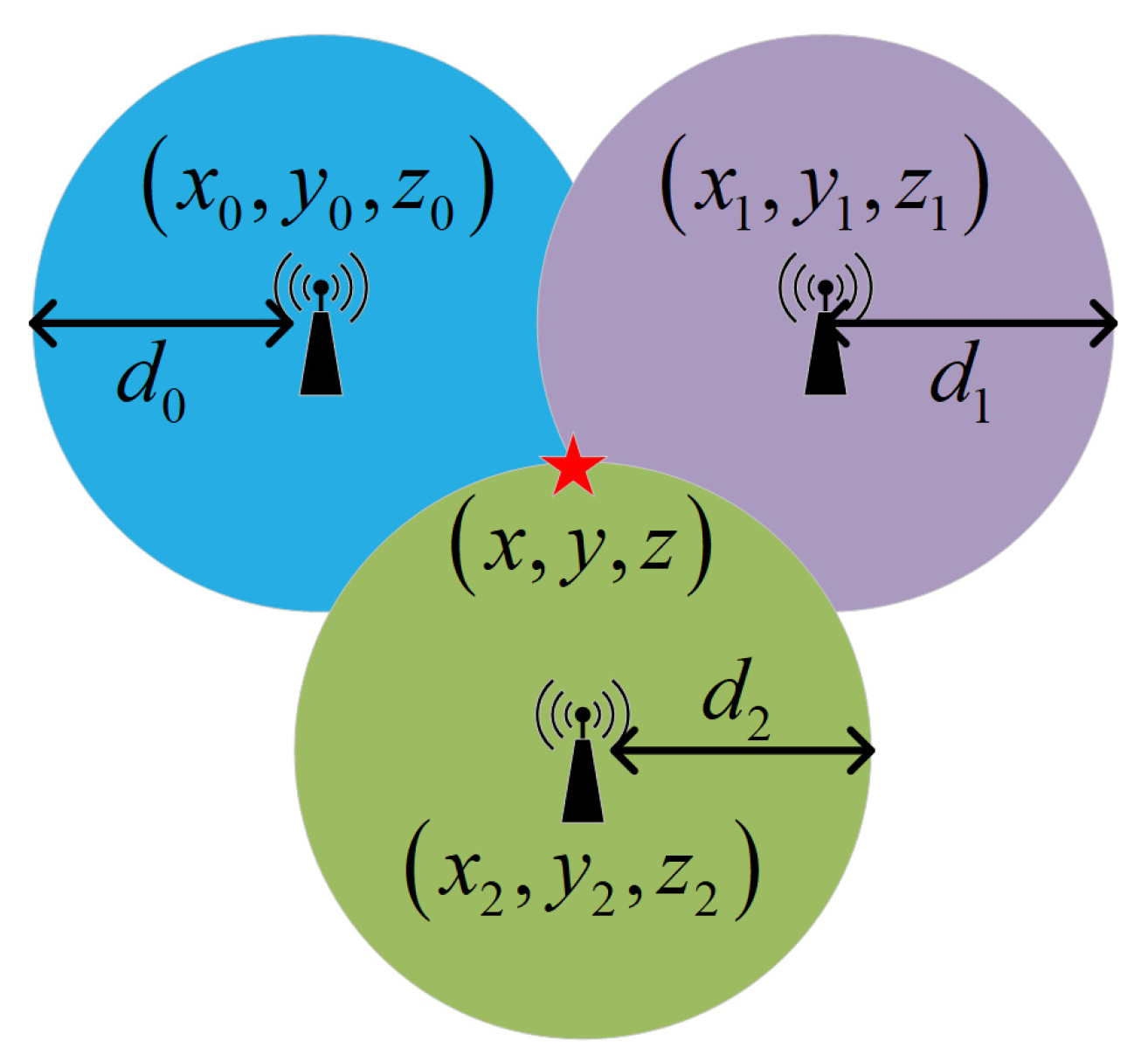
2.2. UWB Measurement Model
- (1)
- Node A transmits a request message to node B while recording the transmission timestamp (referred to as the ranging marker).
- (2)
- Node B receives the request message and records the corresponding reception timestamp . Concurrently, node B sends a response message to node A while recording its transmission timestamp . The time interval between the recorded and at node B is denoted as .
- (3)
- Node A receives the response message and records the corresponding reception timestamp . The time interval between the recorded and at node A is represented as . Subsequently, node A transmits a termination message to node B and records the associated transmission timestamp . The time interval between and is denoted as .
- (4)
- Node B receives the termination message and records the corresponding reception timestamp . The time interval between and is represented as .
2.3. GNSS-RTK Measurement Model
3. Theoretical Analysis of TC INS/UWB/GNSS-RTK Integrated Positioning Model
3.1. State Model
3.2. Measurement Model
3.3. Height Constraint-Aided Model
- (i)
- When wheeled vehicles drive on flat surfaces, they maintain close contact with the ground while moving forward, without any instances of experiencing jump or sideslip within a specified time period [45].
- (ii)
- When vehicles drive in relatively flat regions, the changes in road surface terrain over a given period remain nearly at the same elevation, with only minor variation in height [46].
4. Mathematical Model of VBAKF Under MMCC
4.1. Generalized MMCC
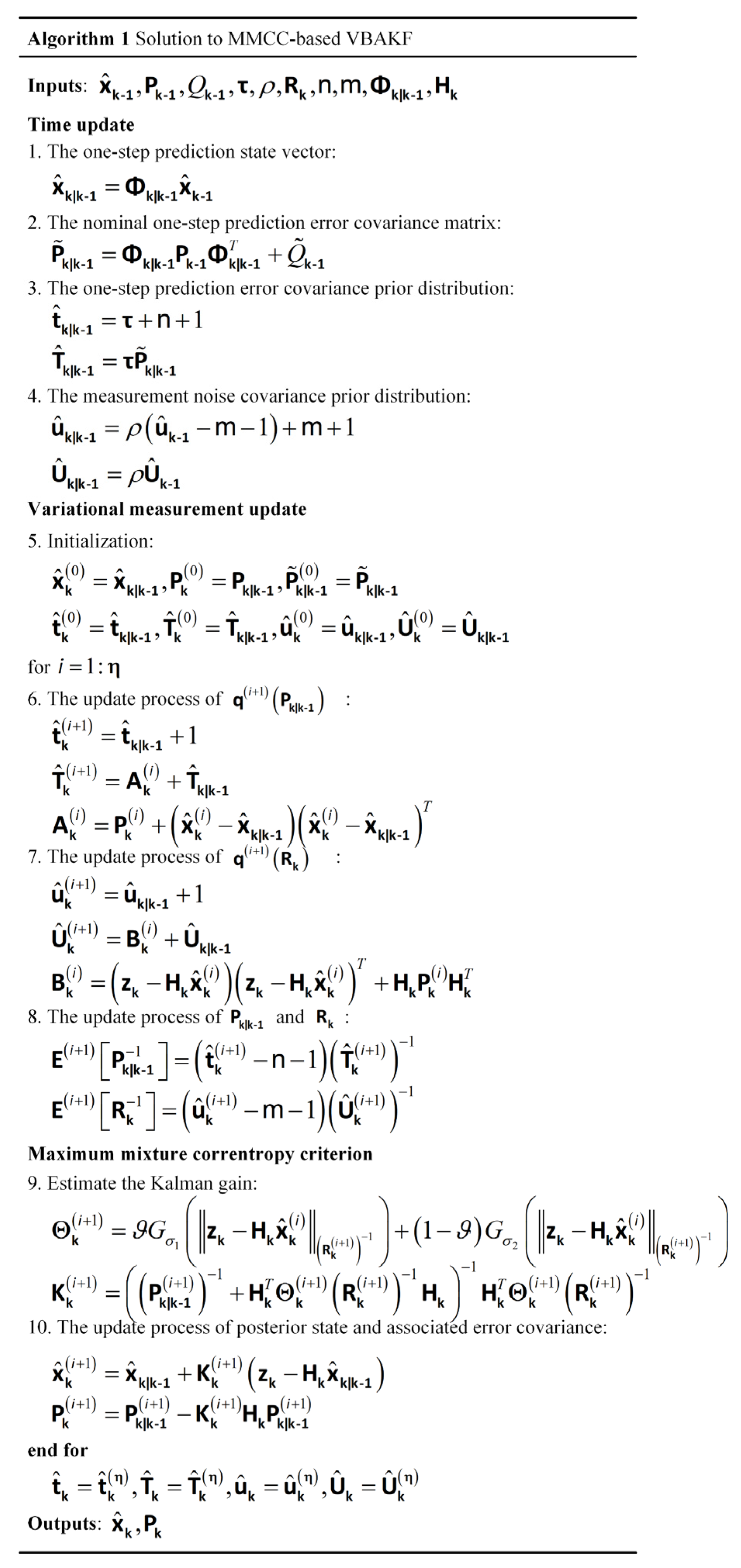
4.2. Derived MMCC-Based VBAKF
5. Experimental Evaluation and Analysis
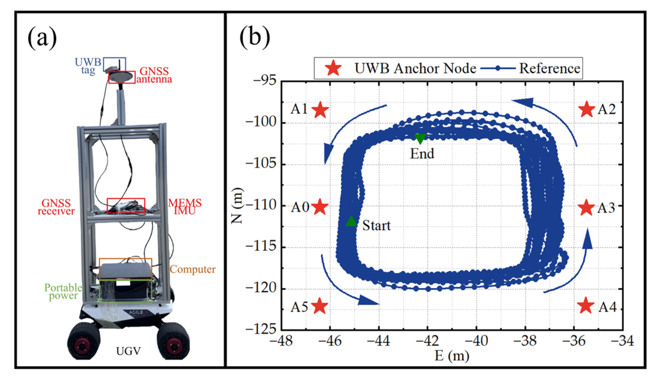
5.1. Equipment Setup and Experiment Description
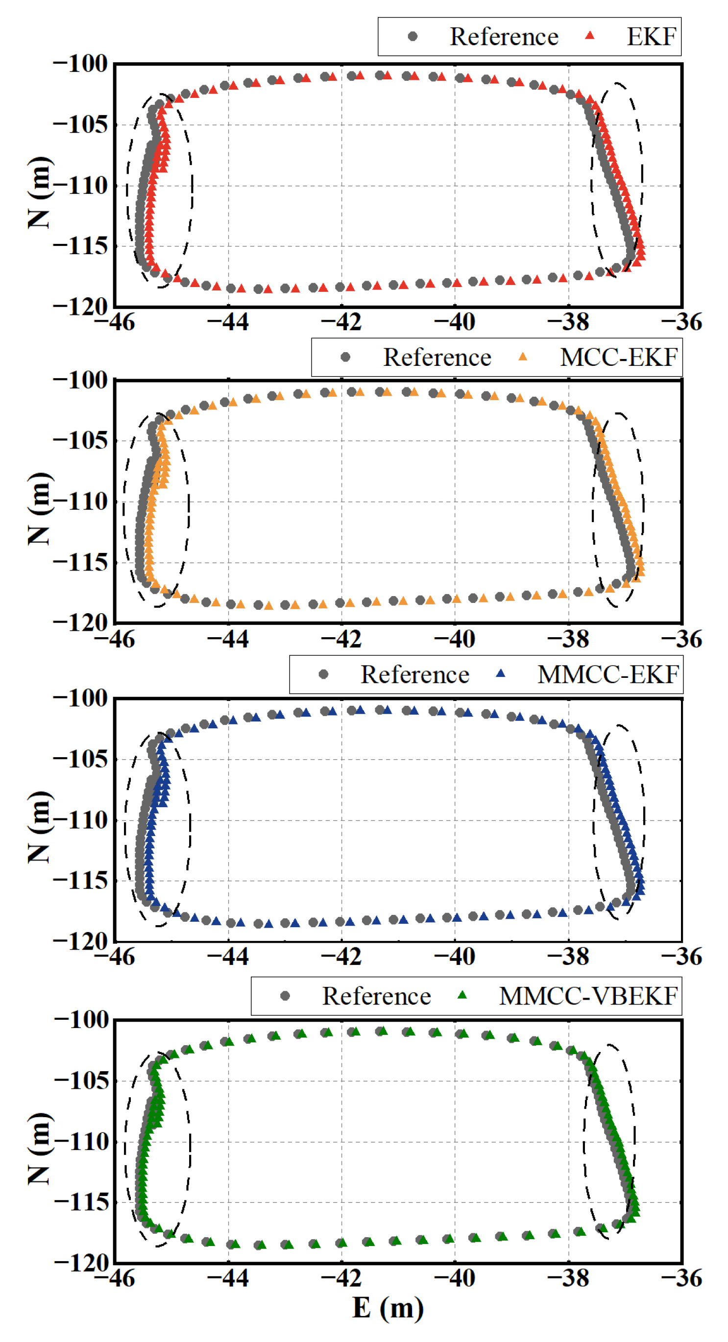
5.2. Positioning Performance Analysis in Real-World Experiment
5.3. Positioning Performance Analysis in Simulation Experiment
6. Conclusions
Author Contributions
Funding
Data Availability Statement
Conflicts of Interest
References
- Qi, L.; Liu, Y.; Yu, Y.; Chen, L.; Chen, R. Current Status and Future Trends of Meter-Level Indoor Positioning Technology: A Review. Remote Sens. 2024, 16, 398. [Google Scholar] [CrossRef]
- Yao, H.; Liang, X.; Chen, R.; Wang, X.; Qi, H.; Chen, L.; Wang, Y. A Benchmark of Absolute and Relative Positioning Solutions in GNSS Denied Environments. IEEE Internet Things J. 2024, 11, 4243–4273. [Google Scholar] [CrossRef]
- Yang, J.; Meng, Z.; Xu, X.; Chen, K.; Li, E.L.; Zhao, P.G.G. Task-Oriented Edge-Assisted Cooperative Data Compression, Communications and Computing for UGV-Enhanced Warehouse Logistics. arXiv 2024, arXiv:2410.01515. Available online: http://arxiv.org/abs/2410.01515 (accessed on 11 October 2024).
- Wei, J.; Fang, Z. An Optimal UAV and UGV Cooperative Network Navigation Algorithm for Bushfire Surveillance and Disaster Relief. In Proceedings of the 2024 16th International Conference on Computer and Automation Engineering (ICCAE), Melbourne, Australia, 14 March 2024; pp. 636–641. [Google Scholar]
- Cai, Z.; Liu, J.; Chi, W.; Zhang, B. A Low-Cost and Robust Multi-Sensor Data Fusion Scheme for Heterogeneous Multi-Robot Cooperative Positioning in Indoor Environments. Remote Sens. 2023, 15, 5584. [Google Scholar] [CrossRef]
- Chi, C.; Zhang, X.; Liu, J.; Sun, Y.; Zhang, Z.; Zhan, X. GICI-LIB: A GNSS/INS/Camera Integrated Navigation Library. IEEE Robot. Autom. Lett. 2023, 8, 7970–7977. [Google Scholar] [CrossRef]
- Li, X.; Ye, J.; Zhang, Z.; Fei, L.; Xia, W.; Wang, B. A Novel Low-Cost UWB/IMU Positioning Method with the Robust Unscented Kalman Filter Based on Maximum Correntropy. IEEE Sens. J. 2024, 24, 29219–29231. [Google Scholar] [CrossRef]
- Zhang, R.; Shen, F.; Liang, Y.; Zhao, D. Using UWB Aided GNSS/INS Integrated Navigation to Bridge GNSS Outages Based on Optimal Anchor Distribution Strategy. In Proceedings of the 2020 IEEE/ION Position, Location and Navigation Symposium (PLANS), Portland, OR, USA, 20–23 April 2020; pp. 1405–1411. [Google Scholar]
- Zhang, Y.; Tan, X.; Zhao, C. UWB/INS Integrated Pedestrian Positioning for Robust Indoor Environments. IEEE Sens. J. 2020, 20, 14401–14409. [Google Scholar] [CrossRef]
- Li, Y.; Gao, Z.; Yang, C.; Xu, Q. A Novel UWB/INS Tight Integration Model Based on Ranging Offset Calibration and Robust Cubature Kalman Filter. Measurement 2024, 237, 115186. [Google Scholar] [CrossRef]
- Han, X.; Hu, Y.; Xie, A.; Yan, X.; Wang, X.; Pei, C.; Zhang, D. Quadratic-Kalman-Filter-Based Sensor Fault Detection Approach for Unmanned Aerial Vehicles. IEEE Sens. J. 2022, 22, 18669–18683. [Google Scholar] [CrossRef]
- Jiang, C.; Zhang, S.; Li, H.; Li, Z. Performance Evaluation of the Filters with Adaptive Factor and Fading Factor for GNSS/INS Integrated Systems. GPS Solut. 2021, 25, 130. [Google Scholar] [CrossRef]
- Gao, H.; Wang, J.; Cui, B.; Wang, X.; Lin, W. An Innovation Gain-Adaptive Kalman Filter for Unmanned Vibratory Roller Positioning. Measurement 2022, 203, 111900. [Google Scholar] [CrossRef]
- Huang, Y.; Zhang, Y.; Wu, Z.; Li, N.; Chambers, J. A Novel Adaptive Kalman Filter with Inaccurate Process and Measurement Noise Covariance Matrices. IEEE Trans. Automat. Contr. 2018, 63, 594–601. [Google Scholar] [CrossRef]
- Xu, B.; Zhang, J.; Razzaqi, A.A. A Novel Robust Filter for Outliers and Time-Varying Delay on an SINS/USBL Integrated Navigation Model. Meas. Sci. Technol. 2021, 32, 015903. [Google Scholar] [CrossRef]
- Liu, C.; Tan, J.; Huang, Z. Maximum Correntropy Criterion-Based Blind Deconvolution and Its Application for Bearing Fault Detection. Measurement 2022, 191, 110740. [Google Scholar] [CrossRef]
- Zhao, S.; Zhou, Y.; Huang, T. A Novel Method for AI-Assisted INS/GNSS Navigation System Based on CNN-GRU and CKF during GNSS Outage. Remote Sens. 2022, 14, 4494. [Google Scholar] [CrossRef]
- Jing, H.; Gao, Y.; Shahbeigi, S.; Dianati, M. Integrity Monitoring of GNSS/INS Based Positioning Systems for Autonomous Vehicles: State-of-the-Art and Open Challenges. IEEE Trans. Intell. Transport. Syst. 2022, 23, 14166–14187. [Google Scholar] [CrossRef]
- Sun, Y.; Li, Z.; Yang, Z.; Shao, K.; Chen, W. Motion Model-Assisted GNSS/MEMS-IMU Integrated Navigation System for Land Vehicle. GPS Solut. 2022, 26, 131. [Google Scholar] [CrossRef]
- Abdolkarimi, E.S.; Mosavi, M.R. Wavelet-Adaptive Neural Subtractive Clustering Fuzzy Inference System to Enhance Low-Cost and High-Speed INS/GPS Navigation System. GPS Solut. 2020, 24, 36. [Google Scholar] [CrossRef]
- Xu, Q.; Gao, Z.; Lv, J.; Yang, C. Tightly Coupled Integration of BDS-3 B2b RTK, IMU, Odometer, and Dual-Antenna Attitude. IEEE Internet Things J. 2023, 10, 6415–6427. [Google Scholar] [CrossRef]
- Liao, J.; Li, X.; Wang, X.; Li, S.; Wang, H. Enhancing Navigation Performance through Visual-Inertial Odometry in GNSS-Degraded Environment. GPS Solut. 2021, 25, 50. [Google Scholar] [CrossRef]
- Yang, X.; Wang, J.; Song, D.; Feng, B.; Ye, H. A Novel NLOS Error Compensation Method Based IMU for UWB Indoor Positioning System. IEEE Sens. J. 2021, 21, 11203–11212. [Google Scholar] [CrossRef]
- Domuta, I.; Palade, T.P. Two-Way Ranging Algorithms for Clock Error Compensation. IEEE Trans. Veh. Technol. 2021, 70, 8237–8250. [Google Scholar] [CrossRef]
- Kok, M.; Hol, J.D.; Schon, T.B. Indoor Positioning Using Ultrawideband and Inertial Measurements. IEEE Trans. Veh. Technol. 2015, 64, 1293–1303. [Google Scholar] [CrossRef]
- Martalo, M.; Perri, S.; Verdano, G.; De Mola, F.; Monica, F.; Ferrari, G. Improved UWB TDoA-Based Positioning Using a Single Hotspot for Industrial IoT Applications. IEEE Trans. Ind. Inf. 2022, 18, 3915–3925. [Google Scholar] [CrossRef]
- Zhong, C.-M.; Lin, R.-H.; Zhu, H.-L.; Lin, Y.-H.; Zheng, X.; Zhu, L.-H.; Gao, Y.-L.; Zhuang, J.-B.; Hu, H.-Q.; Lu, Y.-J.; et al. UWB-Based AOA Indoor Position-Tracking System and Data Processing Algorithm. IEEE Sens. J. 2024, 24, 30522–30529. [Google Scholar] [CrossRef]
- Yao, H.; Shu, H.; Liang, X.; Yan, H.; Sun, H. Integrity Monitoring for Bluetooth Low Energy Beacons RSSI Based Indoor Positioning. IEEE Access 2020, 8, 215173–215191. [Google Scholar] [CrossRef]
- Van Herbruggen, B.; Luchie, S.; Wilssens, R.; De Poorter, E. Single Anchor Localization by Combining UWB Angle-of-Arrival and Two-Way-Ranging: An Experimental Evaluation of the DW3000. In Proceedings of the 2024 International Conference on Localization and GNSS (ICL-GNSS), Antwerp, Belgium, 25 June 2024; pp. 1–7. [Google Scholar]
- Flueratoru, L.; Wehrli, S.; Magno, M.; Lohan, E.S.; Niculescu, D. High-Accuracy Ranging and Localization with Ultrawideband Communications for Energy-Constrained Devices. IEEE Internet Things J. 2022, 9, 7463–7480. [Google Scholar] [CrossRef]
- Li, D.; Wang, X.; Chen, D.; Zhang, Q.; Yang, Y. A Precise Ultra-Wideband Ranging Method Using Pre-Corrected Strategy and Particle Swarm Optimization Algorithm. Measurement 2022, 194, 110966. [Google Scholar] [CrossRef]
- Wang, S.; Dong, X.; Liu, G.; Gao, M.; Xiao, G.; Zhao, W.; Lv, D. GNSS RTK/UWB/DBA Fusion Positioning Method and Its Performance Evaluation. Remote Sens. 2022, 14, 5928. [Google Scholar] [CrossRef]
- Li, X.; Li, S.; Zhou, Y.; Shen, Z.; Wang, X.; Li, X.; Wen, W. Continuous and Precise Positioning in Urban Environments by Tightly Coupled Integration of GNSS, INS and Vision. IEEE Robot. Autom. Lett. 2022, 7, 11458–11465. [Google Scholar] [CrossRef]
- Li, B.; Chen, G. Improving the Combined GNSS/INS Positioning by Using Tightly Integrated RTK. GPS Solut. 2022, 26, 144. [Google Scholar] [CrossRef]
- Xue, X.; Qin, H.; Lu, H. High-Precision Time Synchronization of Kinematic Navigation System Using GNSS RTK Differential Carrier Phase Time Transfer. Measurement 2021, 176, 109132. [Google Scholar] [CrossRef]
- Sahmoudi, M.; Landry, R. A Nonlinear Filtering Approach for Robust Multi-GNSS RTK Positioning in Presence of Multipath and Ionospheric Delays. IEEE J. Sel. Top. Signal Process. 2009, 3, 764–776. [Google Scholar] [CrossRef]
- Tao, X.; Liu, W.; Wang, Y.; Li, L.; Zhu, F.; Zhang, X. Smartphone RTK Positioning with Multi-Frequency and Multi-Constellation Raw Observations: GPS L1/L5, Galileo E1/E5a, BDS B1I/B1C/B2a. J. Geod. 2023, 97, 43. [Google Scholar] [CrossRef]
- Jiang, W.; Cao, Z.; Cai, B.; Li, B.; Wang, J. Indoor and Outdoor Seamless Positioning Method Using UWB Enhanced Multi-Sensor Tightly-Coupled Integration. IEEE Trans. Veh. Technol. 2021, 70, 10633–10645. [Google Scholar] [CrossRef]
- Li, X.; Wu, Z.; Shen, Z.; Xu, Z.; Li, X.; Li, S.; Han, J. An Indoor and Outdoor Seamless Positioning System for Low-Cost UGV Using PPP/INS/UWB Tightly Coupled Integration. IEEE Sens. J. 2023, 23, 24895–24906. [Google Scholar] [CrossRef]
- Wang, C.; Xu, A.; Sui, X.; Hao, Y.; Shi, Z.; Chen, Z. A Seamless Navigation System and Applications for Autonomous Vehicles Using a Tightly Coupled GNSS/UWB/INS/Map Integration Scheme. Remote Sens. 2021, 14, 27. [Google Scholar] [CrossRef]
- Shen, Z.; Li, X.; Zhou, Y.; Li, S.; Wu, Z.; Wang, X. Accurate and Capable GNSS-Inertial-Visual Vehicle Navigation via Tightly Coupled Multiple Homogeneous Sensors. IEEE Trans. Automat. Sci. Eng. 2024. early access. [Google Scholar] [CrossRef]
- Li, Z.; Chang, G.; Gao, J.; Wang, J.; Hernandez, A. GPS/UWB/MEMS-IMU Tightly Coupled Navigation with Improved Robust Kalman Filter. Adv. Space Res. 2016, 58, 2424–2434. [Google Scholar] [CrossRef]
- Shen, Z.; Li, X.; Li, X.; Xu, Z.; Wu, Z.; Zhou, Y. Precise and Robust IMU-Centric Vehicle Navigation via Tightly Integrating Multiple Homogeneous GNSS Terminals. IEEE Trans. Instrum. Meas. 2024, 73, 9501214. [Google Scholar] [CrossRef]
- Xiao, Y.; Luo, H.; Zhao, F.; Wu, F.; Gao, X.; Wang, Q.; Cui, L. Residual Attention Network-Based Confidence Estimation Algorithm for Non-Holonomic Constraint in GNSS/INS Integrated Navigation System. IEEE Trans. Veh. Technol. 2021, 70, 11404–11418. [Google Scholar] [CrossRef]
- Wang, D.; Dong, Y.; Li, Z.; Li, Q.; Wu, J. Constrained MEMS-Based GNSS/INS Tightly Coupled System with Robust Kalman Filter for Accurate Land Vehicular Navigation. IEEE Trans. Instrum. Meas. 2020, 69, 5138–5148. [Google Scholar] [CrossRef]
- Vana, S.; Naciri, N.; Bisnath, S. Benefits of Motion Constraining for Robust, Low-Cost, Dual-Frequency GNSS PPP + MEMS IMU Navigation. In Proceedings of the 2020 IEEE/ION Position, Location and Navigation Symposium (PLANS), Portland, OR, USA, 20–23 April 2020; pp. 1093–1103. [Google Scholar]
- Li, X.; Wang, Y. Research on the UWB/IMU Fusion Positioning of Mobile Vehicle Based on Motion Constraints. Acta Geod. Geophys. 2020, 55, 237–255. [Google Scholar] [CrossRef]
- Wang, Y.; Yang, Z.; Wang, Y.; Dinavahi, V.; Liang, J.; Wang, K. Robust Dynamic State Estimation for Power System Based on Adaptive Cubature Kalman Filter with Generalized Correntropy Loss. IEEE Trans. Instrum. Meas. 2022, 71, 9003811. [Google Scholar] [CrossRef]
- Chen, S.; Zhang, Q.; Zhang, T.; Zhang, L.; Peng, L.; Wang, S. Robust State Estimation with Maximum Correntropy Rotating Geometric Unscented Kalman Filter. IEEE Trans. Instrum. Meas. 2022, 71, 2501714. [Google Scholar] [CrossRef]
- Deng, Z.; Shi, L.; Yin, L.; Xia, Y.; Huo, B. UKF Based on Maximum Correntropy Criterion in the Presence of Both Intermittent Observations and Non-Gaussian Noise. IEEE Sens. J. 2020, 20, 7766–7773. [Google Scholar] [CrossRef]
- Bai, S.; Hu, J.; Yan, Y.; Shen, L.; He, Z.; Yin, G. An Integrated Approach for Vehicle State Estimation Under Non-Ideal Conditions Using Adaptive Strong Tracking Maximum Correntropy Criterion EKF. IEEE Trans. Veh. Technol. 2024, 73, 14604–14616. [Google Scholar] [CrossRef]
- Shao, J.; Chen, W.; Zhang, Y.; Yu, F.; Chang, J. Adaptive Multikernel Size-Based Maximum Correntropy Cubature Kalman Filter for the Robust State Estimation. IEEE Sens. J. 2022, 22, 19835–19844. [Google Scholar] [CrossRef]
- Liu, B.; Zhang, X.; Jia, S.; Zou, S.; Tian, D. Variational Bayesian-Based Adaptive Maximum Correntropy Generalized High-Degree Cubature Kalman Filter. Circuits Syst. Signal Process. 2023, 42, 7073–7098. [Google Scholar] [CrossRef]
- Qiao, S.; Fan, Y.; Wang, G.; Mu, D.; He, Z. Maximum Correntropy Criterion Variational Bayesian Adaptive Kalman Filter Based on Strong Tracking with Unknown Noise Covariances. J. Frankl. Inst. 2023, 360, 6515–6536. [Google Scholar] [CrossRef]
- Dong, X.; Chisci, L.; Cai, Y. An Adaptive Variational Bayesian Filter for Nonlinear Multi-Sensor Systems with Unknown Noise Statistics. Signal Process. 2021, 179, 107837. [Google Scholar] [CrossRef]
- Shi, W.; Xu, J.; He, H.; Li, D.; Tang, H.; Lin, E. Fault-Tolerant SINS/HSB/DVL Underwater Integrated Navigation System Based on Variational Bayesian Robust Adaptive Kalman Filter and Adaptive Information Sharing Factor. Measurement 2022, 196, 111225. [Google Scholar] [CrossRef]
- Yang, B.; Du, B.; Li, N.; Li, S.; Shi, Z. Centered Error Entropy-Based Variational Bayesian Adaptive and Robust Kalman Filter. IEEE Trans. Circuits Syst. II 2022, 69, 5179–5183. [Google Scholar] [CrossRef]
- Ismail, S.; Wadi, A.; Abdel-Hafez, M.F.; Hussein, A.A. A Noise-Resilient Observer for Enhanced Surface Temperature Estimation of Li-Ion Battery Cells. IEEE Trans. Transp. Electrific. 2024. early access. [Google Scholar] [CrossRef]
- Hafez, I.; Wadi, A.; Abdel-Hafez, M.F.; Hussein, A.A. Variational Bayesian-Based Maximum Correntropy Cubature Kalman Filter Method for State-of-Charge Estimation of Li-Ion Battery Cells. IEEE Trans. Veh. Technol. 2023, 72, 3090–3104. [Google Scholar] [CrossRef]
- Shao, J.; Chen, W.; Zhang, Y.; Yu, F.; Wang, J. Adaptive Maximum Correntropy Based Robust CKF with Variational Bayesian for Covariance Estimation. Measurement 2022, 202, 111834. [Google Scholar] [CrossRef]
- Zou, A.; Hu, W.; Luo, Y.; Jiang, P. An Improved UWB/IMU Tightly Coupled Positioning Algorithm Study. Sensors 2023, 23, 5918. [Google Scholar] [CrossRef] [PubMed]
- Yang, B.; Yang, E.; Yu, L.; Niu, C. Sensor Fusion-Based UAV Localization System for Low-Cost Autonomous Inspection in Extremely Confined Environments. IEEE Sens. J. 2024, 24, 22144–22155. [Google Scholar] [CrossRef]
- Singandhupe, A.; La, H.M. MCC-EKF for Autonomous Car Security. In Proceedings of the 2020 Fourth IEEE International Conference on Robotic Computing (IRC), Taichung, Taiwan, 9–11 November 2020; pp. 306–313. [Google Scholar]
- Jwo, D.-J.; Lai, C.-H.; Biswal, A.; Cho, T.-S. An Extended Kalman Filter with Mixture Kernel Maximum Correntropy Criterion for GPS Navigation Applications. Trans. Inst. Meas. Control 2024. [Google Scholar] [CrossRef]


| Item | Gyroscope | Accelerometer |
|---|---|---|
| Bias stability | ||
| Measurement range | ||
| Sampling rate | 200 Hz | 200 Hz |
| Angular random walk | - | |
| Velocity random walk | - |
| Method | EKF | MCC-EKF | MMCC-EKF | MMCC-VBAKF | |
|---|---|---|---|---|---|
| RMSE (m) | E | 0.116 | 0.106 | 0.093 | 0.046 |
| N | 0.059 | 0.040 | 0.039 | 0.029 | |
| U | 0.030 | 0.030 | 0.030 | 0.030 | |
| 2D | 0.130 | 0.114 | 0.101 | 0.054 | |
| MAE (m) | E | 0.106 | 0.097 | 0.085 | 0.042 |
| N | 0.053 | 0.033 | 0.033 | 0.025 | |
| U | 0.024 | 0.023 | 0.023 | 0.023 | |
| 2D | 0.123 | 0.104 | 0.093 | 0.052 | |
| STD (m) | E | 0.048 | 0.085 | 0.039 | 0.022 |
| N | 0.026 | 0.026 | 0.025 | 0.025 | |
| U | 0.030 | 0.030 | 0.030 | 0.030 | |
| 2D | 0.040 | 0.045 | 0.039 | 0.015 | |
| Method | Improvements | ||||||||
|---|---|---|---|---|---|---|---|---|---|
| RMSE (%) | MAE (%) | STD (%) | |||||||
| E | N | 2D | E | N | 2D | E | N | 2D | |
| EKF | 60.34 | 50.85 | 58.46 | 60.38 | 52.83 | 57.72 | 54.17 | 3.85 | 62.50 |
| MCC-EKF | 56.60 | 27.50 | 52.63 | 56.70 | 24.24 | 50.00 | 74.12 | 3.85 | 66.67 |
| MMCC-EKF | 50.54 | 25.64 | 46.53 | 50.59 | 24.24 | 44.09 | 43.59 | 0.00 | 61.54 |
| Method | EKF | MCC-EKF | MMCC-EKF | MMCC-VBAKF | |
|---|---|---|---|---|---|
| RMSE (m) | E | 0.917 | 0.428 | 0.280 | 0.268 |
| N | 1.626 | 1.540 | 1.450 | 0.727 | |
| U | 0.030 | 0.030 | 0.030 | 0.030 | |
| 2D | 1.867 | 1.598 | 1.477 | 0.774 | |
| MAE (m) | E | 0.898 | 0.404 | 0.264 | 0.245 |
| N | 1.541 | 1.455 | 1.362 | 0.671 | |
| U | 0.023 | 0.025 | 0.024 | 0.024 | |
| 2D | 1.821 | 1.532 | 1.395 | 0.726 | |
| STD (m) | E | 0.184 | 0.189 | 0.161 | 0.116 |
| N | 0.520 | 0.505 | 0.500 | 0.279 | |
| U | 0.030 | 0.030 | 0.030 | 0.030 | |
| 2D | 0.412 | 0.454 | 0.395 | 0.269 | |
| Method | Improvements | ||||||||
|---|---|---|---|---|---|---|---|---|---|
| RMSE (%) | MAE (%) | STD (%) | |||||||
| E | N | 2D | E | N | 2D | E | N | 2D | |
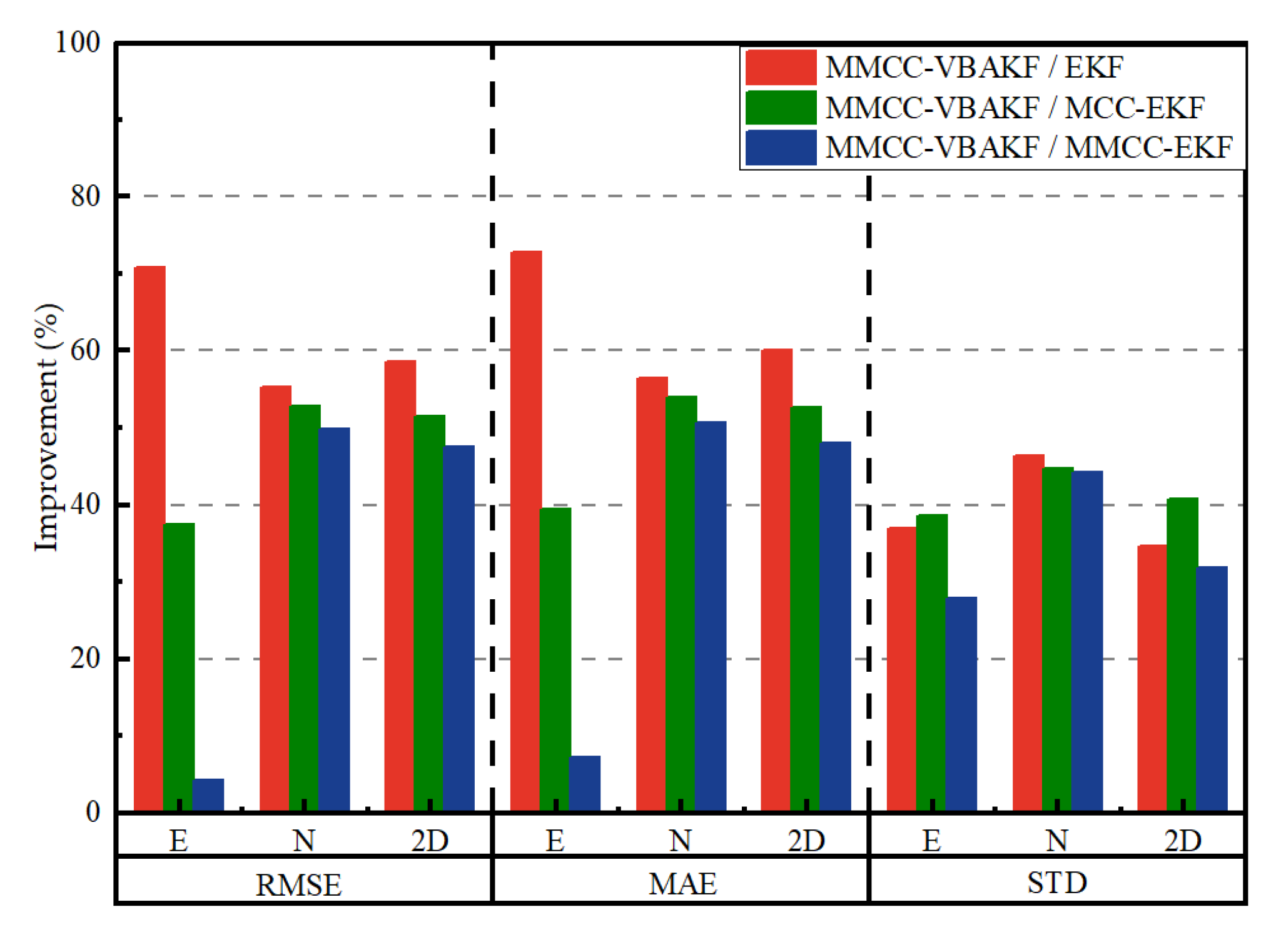
| EKF | 70.77 | 55.29 | 58.54 | 72.72 | 56.46 | 60.13 | 36.96 | 46.35 | 34.71 |
| MCC-EKF | 37.38 | 52.79 | 51.56 | 39.36 | 53.88 | 52.61 | 38.62 | 44.75 | 40.75 |
| MMCC-EKF | 4.29 | 49.86 | 47.60 | 7.20 | 50.73 | 47.96 | 27.95 | 44.20 | 31.90 |
Disclaimer/Publisher’s Note: The statements, opinions and data contained in all publications are solely those of the individual author(s) and contributor(s) and not of MDPI and/or the editor(s). MDPI and/or the editor(s) disclaim responsibility for any injury to people or property resulting from any ideas, methods, instructions or products referred to in the content. |
© 2025 by the authors. Licensee MDPI, Basel, Switzerland. This article is an open access article distributed under the terms and conditions of the Creative Commons Attribution (CC BY) license (https://creativecommons.org/licenses/by/4.0/).
Share and Cite
Wang, S.; Dai, P.; Xu, T.; Nie, W.; Cong, Y.; Xing, J.; Gao, F. Maximum Mixture Correntropy Criterion-Based Variational Bayesian Adaptive Kalman Filter for INS/UWB/GNSS-RTK Integrated Positioning. Remote Sens. 2025, 17, 207. https://doi.org/10.3390/rs17020207
Wang S, Dai P, Xu T, Nie W, Cong Y, Xing J, Gao F. Maximum Mixture Correntropy Criterion-Based Variational Bayesian Adaptive Kalman Filter for INS/UWB/GNSS-RTK Integrated Positioning. Remote Sensing. 2025; 17(2):207. https://doi.org/10.3390/rs17020207
Chicago/Turabian StyleWang, Sen, Peipei Dai, Tianhe Xu, Wenfeng Nie, Yangzi Cong, Jianping Xing, and Fan Gao. 2025. "Maximum Mixture Correntropy Criterion-Based Variational Bayesian Adaptive Kalman Filter for INS/UWB/GNSS-RTK Integrated Positioning" Remote Sensing 17, no. 2: 207. https://doi.org/10.3390/rs17020207
APA StyleWang, S., Dai, P., Xu, T., Nie, W., Cong, Y., Xing, J., & Gao, F. (2025). Maximum Mixture Correntropy Criterion-Based Variational Bayesian Adaptive Kalman Filter for INS/UWB/GNSS-RTK Integrated Positioning. Remote Sensing, 17(2), 207. https://doi.org/10.3390/rs17020207