DRAF-Net: Dual-Branch Residual-Guided Multi-View Attention Fusion Network for Station-Level Numerical Weather Prediction Correction

Abstract

Accurate station-level numerical weather predictions are critical for disaster prevention and mitigation, with error correction playing an essential role. However, existing correction models struggle to effectively handle the high-dimensional features and complex dependencies inherent in meteorological data. To address these challenges, this paper proposes the dual-branch residual-guided multi-view attention fusion network (DRAF-Net), a novel deep learning-based correction model. DRAF-Net introduces two key innovations: (1) a dual-branch residual structure that enhances the spatial sensitivity of deep high-dimensional features and improves output stability by connecting raw data and shallow features to deep features, respectively; and (2) a multi-view attention fusion mechanism that models spatiotemporal influences, temporal dynamics, and spatial associations, significantly improving the representation of complex dependencies. The effectiveness of DRAF-Net was validated on two real-world datasets comprising observations and predictions from Chinese meteorological stations. It achieved an average RMSE reduction of 83.44% and an average MAE reduction of 84.21% across all eight variables, significantly outperforming other methods. Moreover, extensive studies confirmed the critical contributions of each key component, while visualization results highlighted the model’s ability to eliminate anomalous values and improve prediction consistency. The code will be made publicly available to support future research and development.

1. Introduction

Numerical weather prediction (NWP), which forecasts future weather conditions through numerical simulations based on partial differential equations that describe atmospheric processes, serves as the cornerstone of modern meteorological forecasting systems [1,2]. Station-level results are typically obtained by interpolating global or regional gridded predictions and integrating observational data from individual meteorological stations [3]. Accurate station-level predictions are essential not only for preventing and mitigating small-scale meteorological disasters such as heavy rainfall, ice storms, and floods [4], but also for supporting key industries, including port transportation [5], agricultural production [6], and wind power generation [7].

Despite their importance, conventional gridded models, which often have low spatiotemporal resolution, are unable to provide the fine-scale resolution required for station-level predictions [8]. Moreover, the inherently chaotic nature of atmospheric systems constrains the accuracy of these predictions. Consequently, even after incorporating station-level observations, significant errors remain, necessitating additional error correction [9].

Earlier methods for station-level NWP error correction primarily relied on historical statistical information [10,11], anomaly filtering [12], and other rule-based techniques, yet these approaches often exhibited limited generalization capabilities. With the advent of artificial intelligence, machine learning (ML)-based methods emerged as compelling alternatives. Tan et al. [13] were among the first to employ a LightGBM [14] model for temperature correction, demonstrating notable improvements in station-level prediction accuracy. Subsequently, various ML algorithms—including linear regression, LASSO regression, random forest, decision trees, XGBoost [15], and stacking ensembles—have been widely adopted to refine key meteorological variables [16,17,18,19,20,21,22,23,24] such as near-surface wind fields and 2 m temperatures. Despite these advancements, ML-based methods still face intrinsic challenges. They struggle to effectively handle high-dimensional features, making it difficult to capture the intricate spatiotemporal dependencies in station-level meteorological data—an aspect critical for error correction. Moreover, most ML-based approaches are task-specific, focusing on single-variable corrections rather than providing a more comprehensive solution. These limitations ultimately restrict both model performance and practical applicability within integrated forecasting systems.

In recent years, as interdisciplinary research between deep learning (DL) and meteorology has advanced [25,26,27,28,29,30], DL-based models have demonstrated remarkable abilities for exploring and modeling the complex dependencies in meteorological data. Furthermore, neural network models offer significant flexibility and generalization capabilities, making them well-suited for multivariate tasks. Inspired by these developments, This paper aims to overcome the limitations of existing correction methods by constructing a DL-based model specifically tailored to station-level NWP correction, thereby propelling both artificial intelligence and meteorology forward in tandem.

To achieve this objective, we designed a novel dual-branch residual-guided multi-view attention fusion network (DRAF-Net), built upon the Transformer architecture [31]. DRAF-Net introduces two new techniques to fully leverage DL’s advantages in high-dimensional feature representation and spatiotemporal dependency modeling. First, recognizing the high degree of similarity often observed between input and output data in correction tasks (see Figure 1a), we propose a dual-branch residual structure to guide the decoding process. In this structure, the feature branch enhances the spatiotemporal sensitivity of deep, high-dimensional features, thereby improving overall output fidelity. Meanwhile, the data branch directly passes the original data to the variable-aware output head, enabling incremental modeling of the relationship between input and output. This design reduces the model’s burden of complete reconstruction and ultimately boosts correction performance. Second, existing spatiotemporal modeling methods [32,33,34,35,36,37,38,39,40,41] struggle to address the irregular spatial distribution and complex dependencies inherent in station data, as shown in Figure 1b,c. To tackle this, we propose a multi-view attention fusion mechanism based on self-attention [31], which incorporates different feature dimensions into the batch size to enable independent attention calculations across spatiotemporal, temporal, and spatial views. The resulting outputs are then fused to capture comprehensive spatiotemporal dependencies. Compared with modeling global dependencies using only a global spatiotemporal view, decoupling the temporal and spatial views enhances the model’s sensitivity to temporal dynamics and spatial correlations. Our DRAF-Net supports end-to-end, multivariate training and inference.

To evaluate the correction capability of DRAF-Net, we use two real-world datasets containing both observations and predictions from meteorological stations across China. Extensive comparative experiments demonstrate the effectiveness of DRAF-Net, achieving an average root mean squard error (RMSE) reduction of 83.44% and an average mean absolute error (MAE) reduction of 84.21% across all eight variables. Moreover, ablation studies and further analyses underscore the critical contributions of each proposed technique, highlighting their roles in enhancing the model’s overall performance and robustness.

Contributions: In this study, we employ two real-world station-level meteorological datasets from China to investigate how deep learning can enhance station-level NWP. Specifically, we develop a novel DL-based model, DRAF-Net, which incorporates a dual-branch residual structure and a multi-view attention fusion mechanism to address the critical challenges of representing high-dimensional features and modeling complex spatiotemporal dependencies in station-level correction. Comprehensive experiments demonstrate DRAF-Net’s effectiveness and superiority in improving prediction accuracy. This work not only deepens our understanding of DL-based models for station-level NWP but also offers practical benefits for weather-dependent industries such as disaster prevention and agriculture, thereby advancing both artificial intelligence and meteorology. Moreover, it provides a solid foundation for future research on station-level problems, potentially inspiring new directions in data-driven meteorological studies.

2. Materials and Methods

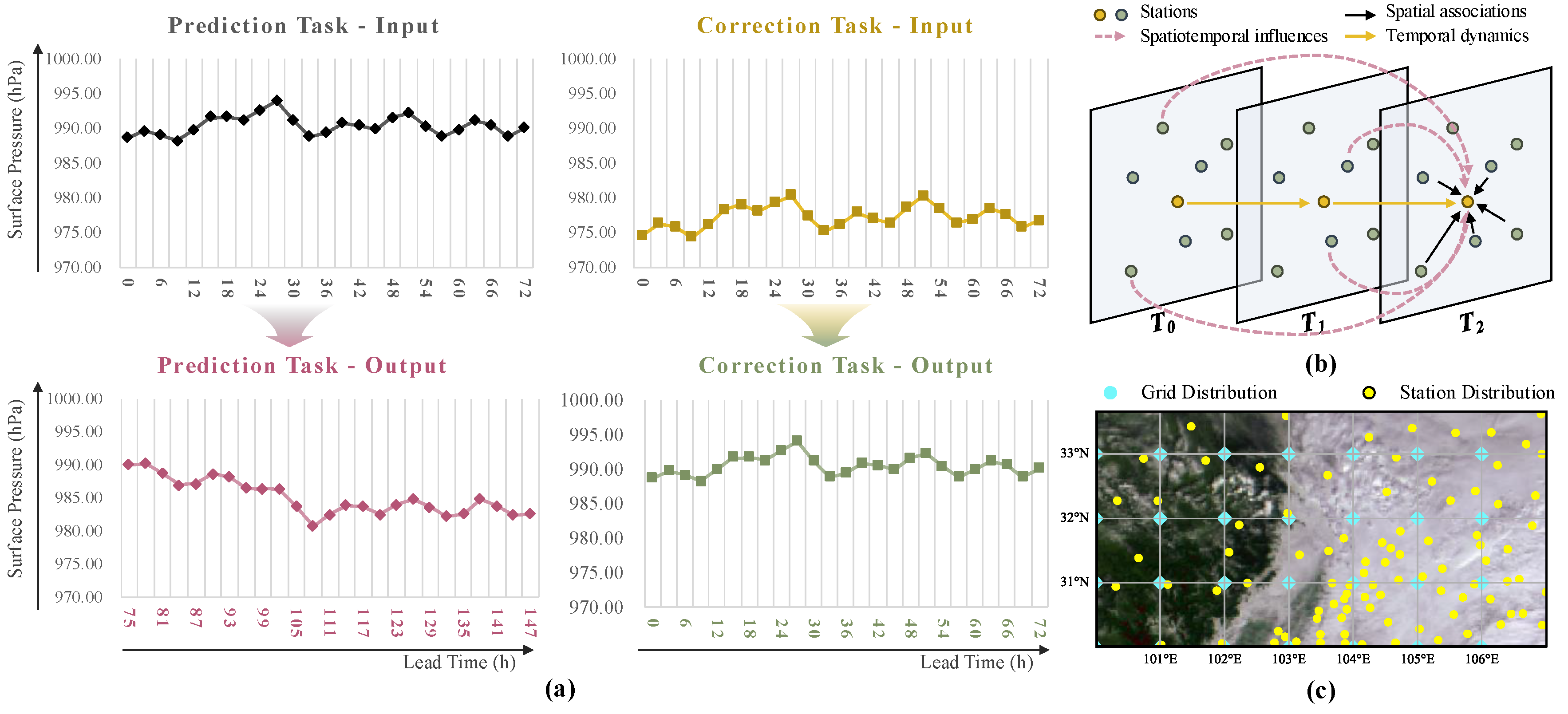
2.1. Datasets

To comprehensively evaluate the correction capabilities of DRAF-Net, we use two real-world datasets comprising observations and predictions for various variables from meteorological stations across China. The first dataset is sourced from an open-access platform [42], supported by the organizing committee of the Tianzhi Cup Artificial Intelligence Challenge. This platform provides high-quality datasets for AI research, covering various domains such as satellite remote sensing, meteorology, radar, and machine power, with the goal of promoting innovation and the application of AI technologies. The dataset includes observations and predictions from 50 meteorological stations, with six common variables: surface pressure, temperature at 2 m, relative humidity at 2 m, wind speed at 10 m, wind direction at 10 m, and visibility. Observations and predictions are recorded at 3 h intervals, with a forecast range of 72 h and initial forecast times at 00:00 or 12:00 UTC. Each prediction run generates 25 files, including the 00-hour lead time. The dataset spans from 1 January 2023 to 3 January 2024. It should be noted that, due to incomplete data sources, some initial forecast times are missing, resulting in the absence of 1250 ($25\times 50$) predictions for each missing time. Additionally, due to occasional instability in ground observation equipment, some data entries are marked as “9999” to indicate invalid values. These invalid entries have been filtered out, and

Table 1. Statistical summary of the first dataset (common variables).

Variable	Abbreviation	Unit	Valid Predictions	Valid Observations
Surface Pressure	p	hpa	653,750	146,195
Temperature at 2 m	t2m	°C	653,750	146,522
Relative Humidity at 2 m	rh2	%	653,750	138,415
Wind Speed at 10 m	ws10	m/s	653,750	146,532
Wind Direction at 10 m	wd10	°	653,750	146,532
Visibility	vis	km	653,750	145,818

provides a statistical summary of the valid data, along with additional details about the dataset.

The second dataset focuses on short-term precipitation forecasting and comprises observations and predictions from 40 meteorological observation stations. It includes 6-h and 24-h accumulated precipitation amounts. Observations and predictions are recorded every 3 h, with a prediction range of 48 h starting at 00:00 UTC each day. Each prediction run generates 17 files, including the 00-hour lead time. This dataset spans from 1 September 2022 to 31 December 2023. It should be noted that, due to incomplete data sources, two initial forecast times are missing, resulting in the absence of 1360 predictions. After removing invalid values,

Table 2. Statistical summary of the second dataset (precipitation variables).

Variable	Abbreviation	Unit	Valid Predictions	Valid Observations
6-h accumulated precipitation	rain6	mm	329,800	142,368
24-h accumulated precipitation	rain24	mm	329,800	109,872

presents a summary of valid entries and further information on this dataset.

We applied two preprocessing steps to both datasets: splitting into training and validation sets, and data standardization. A month-based splitting strategy was adopted to ensure that both the training and validation sets encompass a full range of climate conditions. Specifically, prediction and observation data for forecasts initialized in the last five days of each month were assigned to the validation set, while the remaining data were used for training. Additionally, we computed the mean and variance of the prediction and observation data for each meteorological variable, then applied a zero-mean, unit-variance transformation to standardize the data. This ensures equal contribution of all variables to the model, addressing the issue of scale differences across variables, which could otherwise dominate the learning process. Standardization also improves model convergence by allowing the model to learn more effectively.

2.2. Preliminaries

We formulate the task of error correction for station-level numerical weather predictions as a spatiotemporal regression problem. Specifically, our goal is to train a neural network model M such that, given the station prediction data $P=\{p_1,p_2,p_3,\cdots ,p_V\}\in R^{N\times T}$ as input, the model outputs corrected results $C=\{c_1,c_2,c_3,\cdots ,c_V\}\in R^{N\times T}$ that closely approximate the future observed values $O=\{o_1,o_2,o_3,\cdots ,o_V\}\in R^{N\times T}$. Here, V represents the number of meteorological variables, N denotes the number of observation stations, and T indicates the number of prediction time steps. Unlike general time series or spatiotemporal tasks, this problem poses unique challenges due to the uneven spatial distribution of station data, which complicates the modeling of dependencies.

2.3. Methods

To facilitate a comprehensive understanding of the proposed methods and support further research, this section begins with an overview of the DRAF-Net, followed by detailed explanations of its two primary innovations: the dual-branch residual structure and the multi-view attention fusion mechanism. Finally, we introduce the variable-weighted combined loss function employed to optimize model performance.

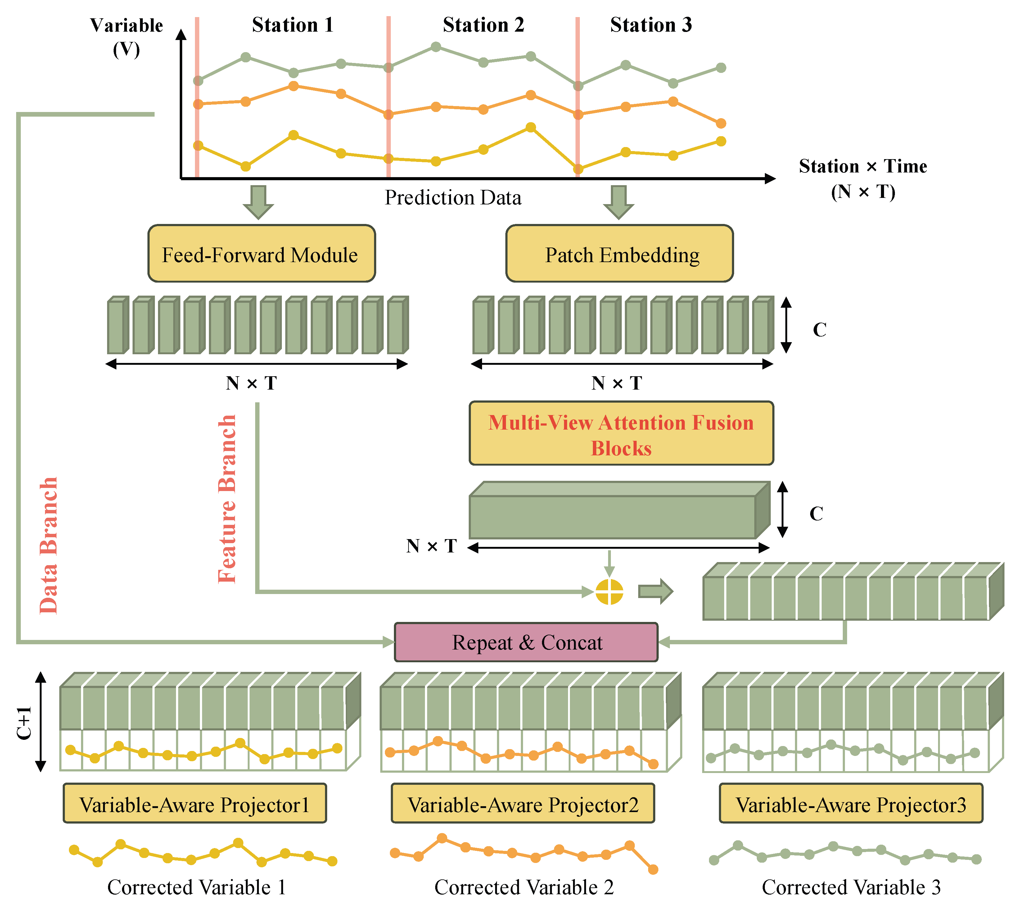
2.3.1. Overview of DRAF-Net

DRAF-Net is built upon the conventional Transformer framework, incorporating specialized design elements to enhance performance on correction tasks and station data, as illustrated in Figure 2. Specifically, the model processes input data, with flattened spatiotemporal dimensions, through a patch embedding module, encoding each spatiotemporal position into high-dimensional representations. Subsequently, multiple Transformer blocks integrated with the multi-view attention fusion mechanism perform feature interactions across three views: spatiotemporal, temporal, and spatial. This approach captures both high-level global dependencies and fine-grained local dependencies, resulting in rich, deep feature representations. To improve output authenticity and stability, DRAF-Net incorporates a dual-branch residual structure. The feature branch enriches deep features with detailed spatiotemporal distribution information via an independent feed-forward module, alleviating the over-smoothing issue caused by multiple layers of feature interaction. Meanwhile, the data branch supplies the original prediction data to the projector, enabling incremental correction. The projector then adjusts the original data based on these enriched features, producing the corrected results. Notably, to account for differences in predictive accuracy across meteorological variables, we employ variable-aware projectors that focus on single-task corrections, thereby improving output accuracy. Through the coordinated operation of these modules, DRAF-Net effectively captures complex dependencies within irregular spatiotemporal data and delivers reliable corrections based on prediction data.

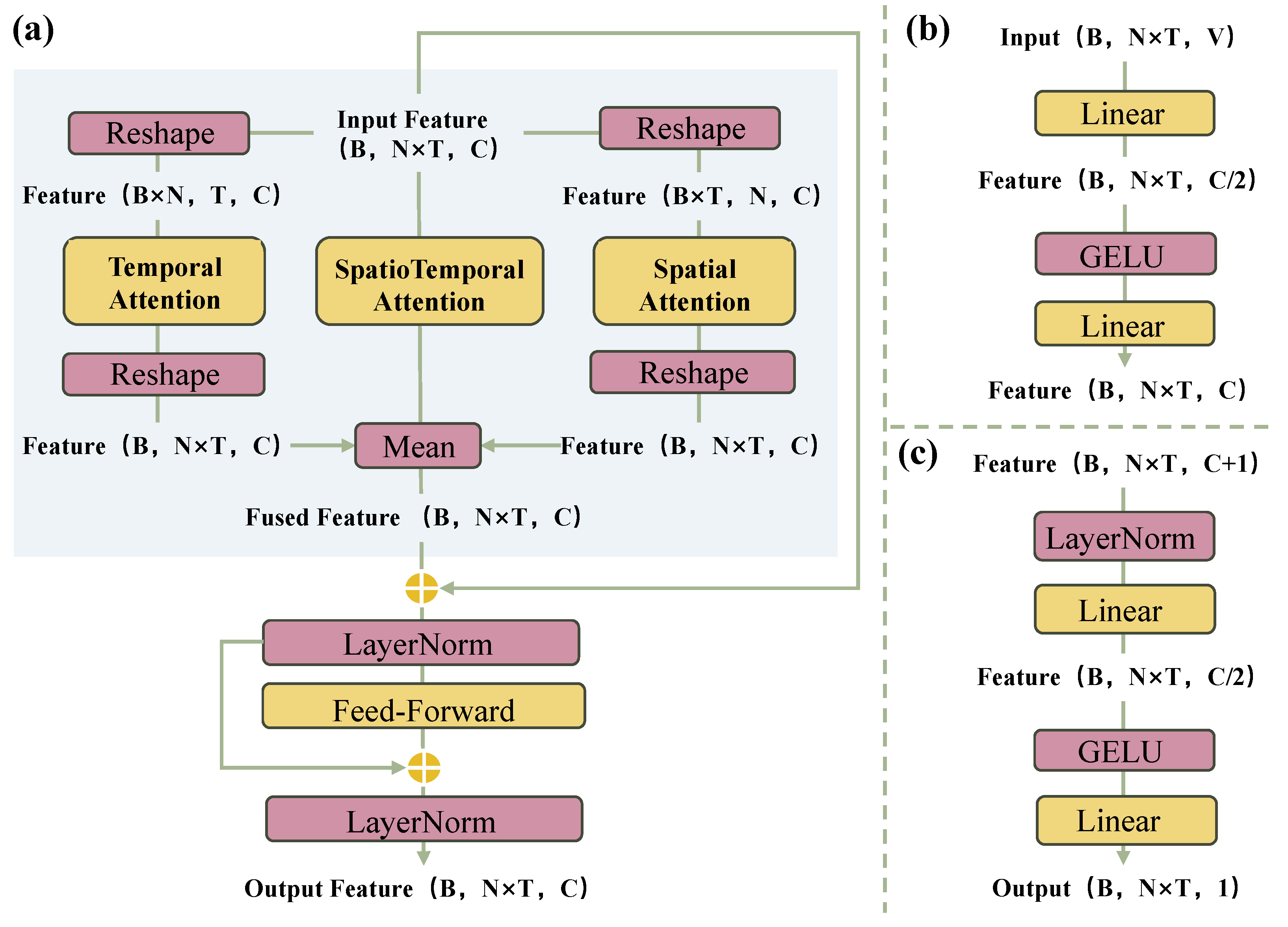
2.3.2. Multi-View Attention Fusion Mechanism

Given the input feature f with dimensions $(B,N\times T,C)$, where B represents the batch size and C is the channel count, our goal is to extract the dependencies among the $N\times T$ features to enhance the model’s understanding of the spatiotemporal contexts, thereby improving its performance in correction tasks. Self-attention mechanisms [31], known for their strong capability to model relationships among sequential features, serve here as the fundamental tool for dependency extraction. The attention calculation is as follows:

$$\mathrm{Attention}(Q,K,V)=\mathrm{softmax}\left({\displaystyle \frac{Q{K}^{\top }}{\sqrt{d_k}}}\right)V,$$

(1)

where $Q=f{W}_Q$, $K=f{W}_K$, and $V=f{W}_V$. Here, $W_Q$, $W_K$, and $W_V$ are learnable matrices that map input features to query, key, and value spaces, respectively. The term $d_k$ represents the dimensionality of the key vectors (K), and it serves as a scaling factor to prevent the dot product between the query (Q) and key (K) from becoming too large, ensuring numerical stability during the attention calculation.

Given that station prediction data involve complex interactions across spatiotemporal influence, temporal variation, and spatial association, we argue that solely applying global modeling to the $N\times T$ dimension may be insufficient. Therefore, we propose a novel multi-view attention fusion mechanism based on self-attention, introducing targeted perspectives from spatiotemporal, temporal, and spatial views to more precisely capture intricate dependencies and dynamic patterns in station prediction data.

To compute attention across different views, we adjust the feature shape to direct the model’s attention focus, as shown in Figure 3a. First, we retain the feature shape as $(B,N\times T,C)$ for spatiotemporal attention. In this view, the model can explore global relationships among all features, capturing cross-spatiotemporal influences among the stations. Next, we decouple the features along the temporal and spatial dimensions to compute attention in the temporal and spatial views separately. For the temporal view, we merge the N dimension into B, resulting in a feature shape of $(B\times N,T,C)$. This enables the model to capture dynamic patterns in meteorological states at each station over time, enhancing its ability to adjust for variations along the temporal dimension. For the spatial view, by merging the T dimension into B, we obtain a feature shape of $(B\times T,N,C)$. This allows the model to focus on feature relationships among different spatial locations at a single time step, capturing spatial dependencies among stations and thereby improving its correction capability for anomalies in the spatial dimension. Finally, we fuse the results from these three perspectives to create a comprehensive feature representation that integrates both global spatiotemporal dependencies and localized temporal and spatial relationships. The fused feature $f_{\mathrm{fused}}$ is computed as follows:

$$f_{\mathrm{fused}}={\displaystyle \frac{1}{3}}({\mathrm{ATT}}_{\mathrm{st}}+{\mathrm{ATT}}_{\mathrm{t}}+{\mathrm{ATT}}_{\mathrm{s}}),$$

(2)

where ${\mathrm{ATT}}_{\mathrm{st}}$, ${\mathrm{ATT}}_{\mathrm{t}}$, and ${\mathrm{ATT}}_{\mathrm{s}}$ represent the attention outputs from the spatiotemporal, temporal, and spatial views, respectively. We apply averaging to prevent numerical inflation, ensuring stability during training.

2.3.3. Dual-Branch Residual Structure

Given the high similarity between input and output data, DRAF-Net introduces two residual connections—a feature branch and a data branch—to address two main challenges faced in decoding: excessive smoothing in the spatiotemporal dimensions of deep features, and the difficulty of directly reconstructing prediction values through the projector.

Firstly, although deep features can represent complex, high-dimensional spatiotemporal dependencies, increasing network depth often leads to excessive smoothing due to repeated fusion computations. This smoothing reduces the model’s sensitivity to fine details, particularly in spatial and temporal positioning, impairing correction accuracy and affecting the authenticity of output results. To counter this issue, we designed the feature branch to compensate for the loss of original spatiotemporal distribution information in deep features. The feature branch employs a shallow neural network with two linear layers (as illustrated in Figure 3b) to encode spatiotemporal information from the original data, injecting this information into the feature stream before the projector. This independent module provides an alternative spatiotemporal representation distinct from the main network and dynamically balances deep and shallow features through learnable weights. This design allows the model to capture high-level information while preserving essential shallow spatiotemporal details, enhancing its ability to retain key information from the input data and resulting in superior performance in correction tasks.

Secondly, we propose that performing bias adjustments based on input data can reduce the model’s burden and improve correction stability and accuracy. Therefore, rather than requiring the projector to reconstruct a prediction result directly from high-dimensional features, we introduce the data branch, which passes the original prediction data for each variable to the variable-aware projector (as shown in Figure 2), enabling incremental correction. The network structure of the variable-aware projector is shown in Figure 3c, and the calculation can be summarized as follows:

$$c_v=W_{v1}{p}_v+W_{v2}{f}_{\mathrm{proj}},$$

(3)

where $W_{v1}$ and $W_{v2}$ are learnable weights within the projector associated with the v-th variable. These weights scale the original data and compute the correction increment. Here, $f_{\mathrm{proj}}$ represents the feature preceding the projector. This approach not only enhances correction accuracy but also significantly improves the model’s optimization efficiency. In summary, the dual-branch residual structure effectively exploits the inherent correlations between input and output data, providing DRAF-Net with enhanced performance and stability in correction tasks.

2.3.4. Overall Loss Function

To mitigate the impact of outliers in the prediction data on the model’s learning process, while preserving the model’s ability to correct such anomalies, we employ a combined loss function incorporating Mmean absolute error (MAE) and mean squared error (MSE). MAE contributes to convergence stability and strengthens the model’s robustness to outliers, while MSE emphasizes larger errors, thereby facilitating the effective correction of anomalies. This combined approach enables the model to balance between normal and abnormal samples, avoiding excessive sensitivity to or disregard for outliers.

Moreover, considering the differences in prediction accuracy and correction difficulty across meteorological variables, we introduce variable-specific weights $w_v$ to balance each variable’s influence on the gradient. This weighting promotes balanced learning in multi-variable contexts and enhances overall correction performance. The variable-weighted combined loss function is defined as follows:

$$\mathcal{L}=\sum _{v=1}^V{w}_v\left(\alpha ·\mathbb{E}|c_v-o_v|+\beta ·\mathbb{E}{(c_v-o_v)}^2\right),$$

(4)

where $\alpha$ and $\beta$ are the weighting coefficients for MAE and MSE, respectively, controlling their relative contributions to the loss function and optimizing the model’s performance across both normal and anomalous data.

3. Experiment

3.1. Experimental Setup

3.1.1. Comparative Experiments

To assess the effectiveness and superiority of our DRAF-Net, we compare it with several mainstream ML-based and DL-based models, which are commonly used for station-level NWP correction and prediction tasks, across two datasets. The original predictions from the NWP model are used as the baseline for comparison. The models used for comparison include linear regression, XGBoost [15], LightGBM [14], and advanced DL-based architectures such as the Transformer [31], FlowFormer [43], Reformer [44], Flashformer [45], Informer [46], and iTransformer [47]. ML models typically accept single-point inputs (V variables) and output the corrected value for a single meteorological variable. Consequently, to handle V meteorological variables, we trained V separate models, each correcting one individual variable. DL models are primarily designed for sequence modeling tasks. However, station-level NWP correction involves both temporal and spatiotemporal dependencies, which these models may not fully account for. To ensure a fair comparison, we evaluate the performance of each DL model using two different input formats: temporal input (V variables over T time steps) and spatiotemporal input (V variables over T time steps for N stations).

3.1.2. Ablation Studies

To understand the contribution of each novel technique introduced in this paper, we conducted a series of ablation studies using the first dataset. The selection criteria for the rejected methods are based on the hypothesized contributions of each individual component to the model’s performance, specifically each branch in the dual-branch residual structure, each view in the multi-view attention mechanism, and each calculation in the element-wise weighted loss function. The reference experiment for all ablation studies is the complete DRAF-Net model, where all components are included. To analyze the costs of rejecting different methods, we evaluated the performance degradation resulting from the removal of individual components or combinations of components. Experiments were designed to isolate the effect of a single element or a set of elements on the overall performance. These ablation studies provide valuable insights into the relative importance of each component in DRAF-Net, demonstrating how they collectively enhance model performance. They also validate the design choices underpinning our approach and guide future improvements in model design.

3.1.3. Alternative Implementation Studies

To validate the rationale behind the dual-branch residual structure, we conducted alternative implementation studies by modifying each branch individually. Specifically, for the feature branch, we replaced the input features with the output from patch embedding, which still preserves spatial representation, while removing the independent feed-forward neural network. For the data branch, we modified the model to directly add the original predictions to the projectors’ output, rather than combining them with the features before passing them to the projectors. The reference experiment for these studies remains the complete DRAF-Net, ensuring consistency across both sets of experiments. This approach allows us to evaluate the function of each implementation in isolation and assess its individual contribution to the overall model performance.

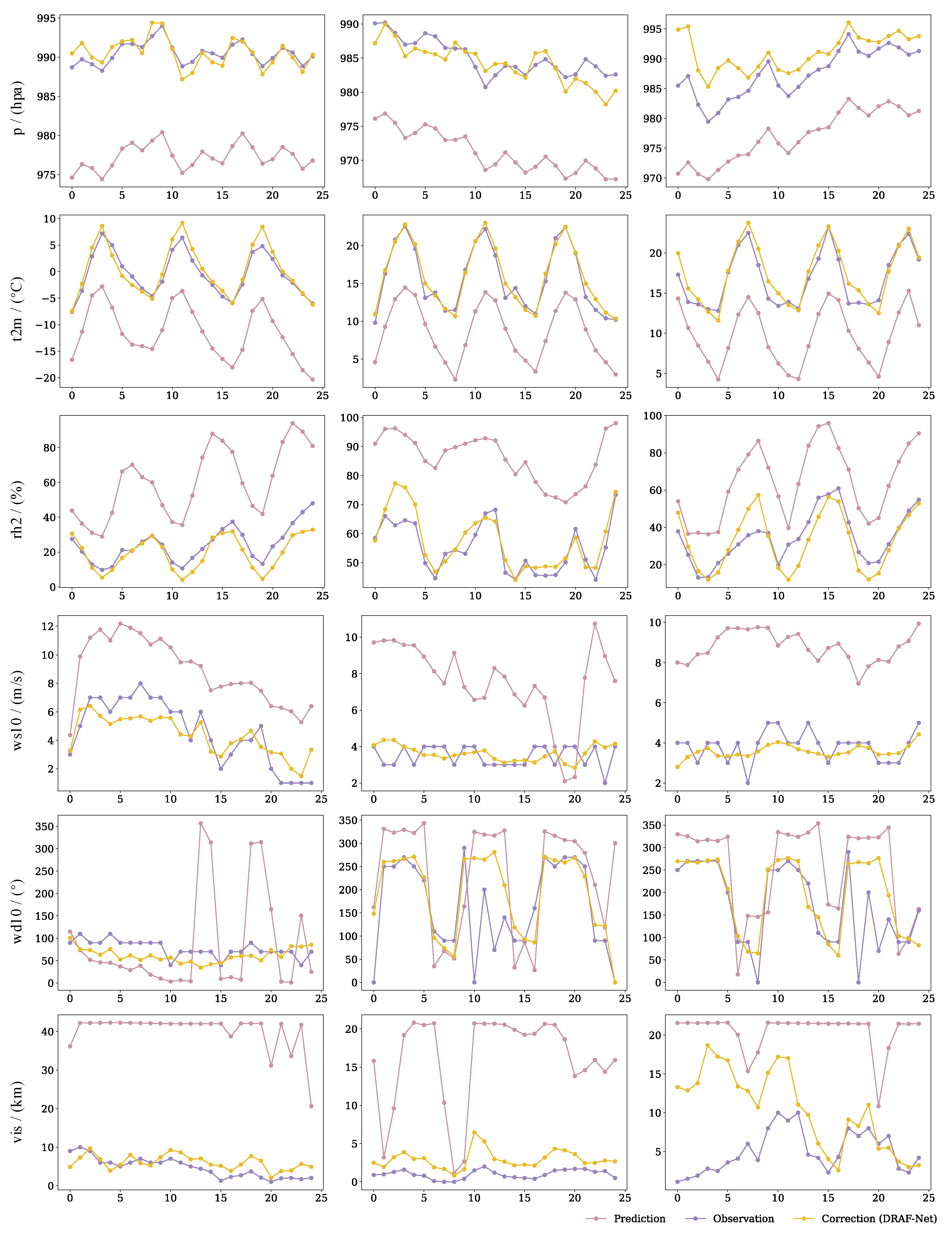
3.1.4. Visualization of Results

To visually illustrate DRAF-Net’s ability to correct station-level NWP, we selected three representative stations for each common meteorological variable from the first dataset and visualized the corresponding observations, predictions, and corrections over 25 consecutive time steps. The results can offer an intuitive comparison between the DRAF-Net’s outputs and the original NWP model predictions, highlighting the model’s correction capability and its effectiveness in improving station-level prediction accuracy.

3.2. Implementation Details

All experiments in this study were implemented using the PyTorch framework and conducted on a single NVIDIA 3090 GPU. The AdamW optimizer [48] was employed for training, with hyperparameters set to ${\beta }_1=0.9$, ${\beta }_2=0.999$, and a weight decay of $5\times {10}^{-5}$. The initial learning rate was set to $5\times {10}^{-4}$, and we employed a combined warm-up and cosine annealing strategy for learning rate scheduling. A batch size of 1 was used, and training was performed for a maximum of 50 epochs. For all DL-based models, the embedding dimension was set to 512, the intermediate feature dimension to 2048, and the number of encoder layers to 3. For the ML-based methods, we implemented three models using the sklearn library [49]. Following standard practices, the maximum depth for tree-based models was set to 6, and the number of iterations was fixed at 100.

3.3. Metrics

Building on previous studies [13,18,28], we evaluate the model’s correction capability using RMSE and MAE, two commonly used metrics for regression error assessment. The formulas are defined as follows:

$$RMSE=\sqrt{\mathbb{E}{\left(c_v-o_v\right)}^2},$$

(5)

$$MAE=\mathbb{E}\left|c_v-o_v\right|.$$

(6)

To provide a more comprehensive evaluation of common variables, we introduce two additional metrics frequently used in hydrological studies: nash-sutcliffe efficiency (NSE) and kling-gupta efficiency (KGE). NSE measures the goodness of fit between model predictions and observations, with values ranging from $(-\infty ,1]$, where values closer to 1 indicate superior performance. KGE evaluates overall agreement by balancing correlation, bias, and variability, with higher values also indicating better performance. Their formulas are as follows:

$$NSE=1-{\displaystyle \frac{\sum {(o_v-c_v)}^2}{\sum {(o_v-\mathbb{E}\left(o_v\right))}^2}},$$

(7)

$$KGE=1-\sqrt{{(r-1)}^2+{(\beta -1)}^2+{(\alpha -1)}^2},$$

(8)

where r denotes the Pearson correlation coefficient between the prediction and observation data, $\beta$ is the ratio of the mean prediction to the mean observation, and $\alpha$ is the ratio of the standard deviation of the prediction to the observation.

For accumulated precipitation, considering the unique characteristics of rainfall events [50] and the public’s greater interest in intensity rather than precise values, We adopted a scoring metric proposed by the Tianzhi Cup platform [42]. This metric assesses prediction performance based on categorized precipitation levels, offering a more intuitive and practical assessment. Accumulated precipitation over 6-h and 24-h periods is categorized into five levels—tiny, light, moderate, heavy, and torrential—using predefined thresholds outlined in

Table 3. Classification of accumulated precipitation by intensity over 6-h and 24-h periods.

Variables	Tiny	Light	Moderate	Heavy	Torrential
Rain6 (mm)	$0.0\sim 0.1$	$0.1\sim 2.4$	$2.5\sim 4.9$	$5.0\sim 9.9$	≥10.0
Rain24 (mm)	$0.0\sim 0.1$	$0.1\sim 9.9$	$10.0\sim 24.9$	$25.0\sim 49.9$	≥50.0

. Once categorized, a scoring system is applied to evaluate the agreement between predicted and observed precipitation levels, as shown in

Table 4. Evaluation scores (%) corresponding to predicted and observed precipitation classification, with the horizontal axis representing observed results and the vertical axis representing predicted results.

Type	Tiny	Light	Middle	Heavy	Torrential
Tiny	100	60	50	40	20
Light	60	100	75	60	30
Middle	50	75	100	80	40
Heavy	40	60	80	100	50
Torrential	20	30	40	50	100

. Accurate predictions are rewarded with high scores, while discrepancies are penalized proportionally. For example, if the model predicts torrential rain but the actual observation indicates light rain, the score is 20. Conversely, a perfect match for torrential rain yields a maximum score of 100. Unlike traditional regression metrics, this scoring system emphasizes the practical importance of accurately capturing precipitation intensities. By aligning with human assessments of rainfall events, it offers a more interpretable evaluation framework.

4. Results

4.1. Comparative Experiments

4.1.1. The First Dataset

Table 5, Table 6, Table 7 and Table 8 present the correction performance of each method across six common meteorological variables, evaluated using various metrics. The results show a similar trend across all metrics. When comparing ML-based and DL-based methods, although the ML-based models demonstrate certain correction capabilities and outperform the baseline, their performance remains significantly lower than that of the DL-based models. This outcome supports the hypothesis presented in the introduction, which suggested that DL methods have the potential to overcome the limitations of ML approaches in station-level correction tasks.

Among the DL methods, when the input data are in a temporal format, Reformer [44] outperforms all other models across all six variables, achieving the best overall performance. In contrast, Informer [46] performs the worst, slightly outperforming iTransformer [47] only in vis. When the input data are converted to a spatiotemporal format, all models—except for the Transformer [31]—experience varying degrees of performance degradation. Notably, the Transformer [31] shows substantial improvement in the spatiotemporal format. As a result, the Transformer [31]’s overall performance improves from the middle rank to the top tier. Except for slight performance losses in MAE for t2m (0.44) and rh2 (1.55), where it slightly lags behind the Reformer [44] scores of 0.43 and 1.54, the Transformer [31] ranks second in all other metrics.

Although the Transformer [31] shows notable improvements, it still falls short of DRAF-Net’s performance. DRAF-Net achieves the best results across all variables and all metrics, confirming that DRAF-Net significantly outperforms existing models in terms of both accuracy and reliability. Compared to the baseline, DRAF-Net shows significant improvement: the averaged RMSE decreases by 28.04 (92.1%), the averaged MAE decreases by 18.44 (91.6%), the averaged NSE increases by 28.01 (102.6%), and the averaged KGE increases by 0.25 (42.3%). These results clearly demonstrate the effectiveness of our proposed method.

4.1.2. The Second Dataset

Table 9 presents the correction errors and scores for accumulated precipitation over 6-h and 24-h periods across different models. The results consistently demonstrate that DRAF-Net outperforms all other models in both time frames. For 6-h accumulated precipitation, DRAF-Net achieves an RMSE of 2.30 and an MAE of 0.52, which represent reductions of 0.17 and 0.32, respectively, compared to the second-best model. Additionally, DRAF-Net achieves the highest overall score of 98.6, further confirming its effectiveness. Similarly, for 24-h accumulated precipitation, DRAF-Net exhibits superior performance, with RMSE and MAE values that are 0.25 and 0.67 lower, respectively, than those of the runner-up. Furthermore, DRAF-Net improves the score by 47.5 and 44.3 points for the two variables, respectively, compared to the baseline. These results further highlight DRAF-Net’s exceptional performance and reliability in challenging correction tasks.

Table 5. Comparison of RMSE values for corrections on six common variables across different models. The best results are highlighted in bold, while the second-best results are underlined. LR represents linear regression, and baseline refers to the original NWP results.

Input Format	Model	p (hpa)	t2m (°C)	rh2 (%)	ws10 (m/s)	wd10 (°)	vis (km)	Mean
-	Baseline	28.80	3.46	15.87	1.91	120.66	12.04	30.46
single-point (V)	LR	24.93	2.84	13.80	1.60	103.04	8.49	25.79
	XGBoost	20.19	2.42	12.45	1.43	97.62	7.60	23.62
	LightGBM	21.00	2.49	12.76	1.46	97.62	7.69	23.84
Temporal ($T,V$)	Transformer	1.51	0.65	2.24	0.96	9.11	2.24	2.79
	Flashformer	1.08	0.73	2.41	0.99	9.21	2.24	2.78
	FlowFormer	1.07	0.70	2.37	0.97	9.16	2.23	2.75
	Informer	1.77	0.87	2.63	1.10	9.68	2.47	3.09
	Reformer	1.03	0.59	2.18	0.94	9.08	2.20	2.67
	iTransformer	1.52	0.69	2.34	1.05	9.70	2.56	2.98
Spatiotemporal ($N\times T,V$)	Transformer	0.51	0.59	2.16	0.90	8.99	2.08	2.54
	Flashformer	2.50	1.93	3.32	1.17	10.07	2.81	3.63
	FlowFormer	2.27	1.78	3.20	1.10	9.43	2.35	3.36
	Informer	2.38	1.91	3.22	1.14	9.92	2.66	3.54
	Reformer	0.64	1.03	3.10	1.11	9.52	2.38	2.96
	iTransformer	0.97	1.27	3.16	1.18	10.27	2.62	3.25
	DRAF-Net	0.24	0.49	2.03	0.88	8.90	2.00	2.42

Table 5. Comparison of RMSE values for corrections on six common variables across different models. The best results are highlighted in bold, while the second-best results are underlined. LR represents linear regression, and baseline refers to the original NWP results.

Input Format	Model	p (hpa)	t2m (°C)	rh2 (%)	ws10 (m/s)	wd10 (°)	vis (km)	Mean
-	Baseline	28.80	3.46	15.87	1.91	120.66	12.04	30.46
single-point (V)	LR	24.93	2.84	13.80	1.60	103.04	8.49	25.79
	XGBoost	20.19	2.42	12.45	1.43	97.62	7.60	23.62
	LightGBM	21.00	2.49	12.76	1.46	97.62	7.69	23.84
Temporal ($T,V$)	Transformer	1.51	0.65	2.24	0.96	9.11	2.24	2.79
	Flashformer	1.08	0.73	2.41	0.99	9.21	2.24	2.78
	FlowFormer	1.07	0.70	2.37	0.97	9.16	2.23	2.75
	Informer	1.77	0.87	2.63	1.10	9.68	2.47	3.09
	Reformer	1.03	0.59	2.18	0.94	9.08	2.20	2.67
	iTransformer	1.52	0.69	2.34	1.05	9.70	2.56	2.98
Spatiotemporal ($N\times T,V$)	Transformer	0.51	0.59	2.16	0.90	8.99	2.08	2.54
	Flashformer	2.50	1.93	3.32	1.17	10.07	2.81	3.63
	FlowFormer	2.27	1.78	3.20	1.10	9.43	2.35	3.36
	Informer	2.38	1.91	3.22	1.14	9.92	2.66	3.54
	Reformer	0.64	1.03	3.10	1.11	9.52	2.38	2.96
	iTransformer	0.97	1.27	3.16	1.18	10.27	2.62	3.25
	DRAF-Net	0.24	0.49	2.03	0.88	8.90	2.00	2.42

Table 6. Comparison of MAE values for corrections on six common variables across different models. The best results are highlighted in bold, while the second-best results are underlined. LR represents linear regression, and baseline refers to the original NWP results.

Input Format	Model	p (hpa)	t2m (°C)	rh2 (%)	ws10 (m/s)	wd10 (°)	vis (km)	Mean
-	Baseline	15.22	2.68	11.93	1.36	80.19	9.48	20.14
Single-point (V)	LR	10.76	2.14	10.58	1.14	82.77	7.19	19.10
	XGBoost	8.15	1.83	9.39	1.03	74.49	6.07	16.83
	LightGBM	8.95	1.88	9.66	1.05	75.04	6.23	17.14
Temporal ($T,V$)	Transformer	0.56	0.48	1.61	0.68	6.65	1.67	1.94
	Flashformer	0.56	0.55	1.75	0.71	6.80	1.68	2.01
	FlowFormer	0.42	0.52	1.71	0.69	6.68	1.64	1.94
	Informer	0.87	0.67	1.99	0.78	7.47	1.97	2.29
	Reformer	0.44	0.43	1.54	0.67	6.61	1.64	1.89
	iTransformer	0.60	0.51	1.72	0.74	7.28	2.01	2.14
Spatiotemporal ($N\times T,V$)	Transformer	0.40	0.44	1.55	0.65	6.46	1.49	1.83
	Flashformer	1.62	1.38	4.10	0.82	8.48	1.89	3.05
	FlowFormer	1.20	1.60	3.34	0.86	8.06	1.75	2.80
	Informer	1.78	1.72	3.49	0.85	8.60	1.69	3.02
	Reformer	0.45	0.78	2.30	0.78	7.46	1.81	2.26
	iTransformer	0.76	0.97	2.45	0.84	7.34	1.84	2.37
	DRAF-Net	0.18	0.36	1.43	0.62	6.23	1.40	1.70

Table 6. Comparison of MAE values for corrections on six common variables across different models. The best results are highlighted in bold, while the second-best results are underlined. LR represents linear regression, and baseline refers to the original NWP results.

Input Format	Model	p (hpa)	t2m (°C)	rh2 (%)	ws10 (m/s)	wd10 (°)	vis (km)	Mean
-	Baseline	15.22	2.68	11.93	1.36	80.19	9.48	20.14
Single-point (V)	LR	10.76	2.14	10.58	1.14	82.77	7.19	19.10
	XGBoost	8.15	1.83	9.39	1.03	74.49	6.07	16.83
	LightGBM	8.95	1.88	9.66	1.05	75.04	6.23	17.14
Temporal ($T,V$)	Transformer	0.56	0.48	1.61	0.68	6.65	1.67	1.94
	Flashformer	0.56	0.55	1.75	0.71	6.80	1.68	2.01
	FlowFormer	0.42	0.52	1.71	0.69	6.68	1.64	1.94
	Informer	0.87	0.67	1.99	0.78	7.47	1.97	2.29
	Reformer	0.44	0.43	1.54	0.67	6.61	1.64	1.89
	iTransformer	0.60	0.51	1.72	0.74	7.28	2.01	2.14
Spatiotemporal ($N\times T,V$)	Transformer	0.40	0.44	1.55	0.65	6.46	1.49	1.83
	Flashformer	1.62	1.38	4.10	0.82	8.48	1.89	3.05
	FlowFormer	1.20	1.60	3.34	0.86	8.06	1.75	2.80
	Informer	1.78	1.72	3.49	0.85	8.60	1.69	3.02
	Reformer	0.45	0.78	2.30	0.78	7.46	1.81	2.26
	iTransformer	0.76	0.97	2.45	0.84	7.34	1.84	2.37
	DRAF-Net	0.18	0.36	1.43	0.62	6.23	1.40	1.70

Table 7. Comparison of NSE for corrections on six common variables across different models. The best results are highlighted in bold, while the second-best results are underlined. LR represents linear regression, and baseline refers to the original NWP results.

Input Format	Model	p	t2m	rh2	ws10	wd10	vis	Mean
-	Baseline	−7.37	0.01	−9.49	−0.91	−132.23	−13.82	−27.30
Single-point (V)	LR	−5.27	0.33	−6.93	−0.35	−96.17	−6.38	-19.13
	XGBoost	−3.11	0.51	−5.45	−0.06	−86.20	−4.91	−16.54
	LightGBM	−3.45	0.48	−5.77	−0.12	−86.22	−5.05	−16.69
Temporal ($T,V$)	Transformer	0.98	0.97	0.79	0.52	0.24	0.49	0.67
	Flashformer	0.99	0.96	0.76	0.49	0.22	0.49	0.65
	FlowFormer	0.99	0.96	0.77	0.51	0.23	0.49	0.66
	Informer	0.97	0.94	0.71	0.37	0.14	0.38	0.59
	Reformer	0.99	0.97	0.80	0.54	0.25	0.50	0.68
	iTransformer	0.98	0.96	0.77	0.43	0.14	0.33	0.60
Spatiotemporal ($N\times T,V$)	Transformer	0.99	0.97	0.81	0.57	0.26	0.56	0.69
	Flashformer	0.94	0.69	0.54	0.29	0.07	0.20	0.46
	FlowFormer	0.95	0.74	0.57	0.37	0.19	0.44	0.54
	Informer	0.94	0.70	0.57	0.33	0.10	0.28	0.49
	Reformer	0.99	0.91	0.60	0.36	0.17	0.42	0.58
	iTransformer	0.99	0.87	0.58	0.27	0.03	0.30	0.51
	DRAF-Net	1.00	0.98	0.83	0.59	0.28	0.59	0.71

Table 7. Comparison of NSE for corrections on six common variables across different models. The best results are highlighted in bold, while the second-best results are underlined. LR represents linear regression, and baseline refers to the original NWP results.

Input Format	Model	p	t2m	rh2	ws10	wd10	vis	Mean
-	Baseline	−7.37	0.01	−9.49	−0.91	−132.23	−13.82	−27.30
Single-point (V)	LR	−5.27	0.33	−6.93	−0.35	−96.17	−6.38	-19.13
	XGBoost	−3.11	0.51	−5.45	−0.06	−86.20	−4.91	−16.54
	LightGBM	−3.45	0.48	−5.77	−0.12	−86.22	−5.05	−16.69
Temporal ($T,V$)	Transformer	0.98	0.97	0.79	0.52	0.24	0.49	0.67
	Flashformer	0.99	0.96	0.76	0.49	0.22	0.49	0.65
	FlowFormer	0.99	0.96	0.77	0.51	0.23	0.49	0.66
	Informer	0.97	0.94	0.71	0.37	0.14	0.38	0.59
	Reformer	0.99	0.97	0.80	0.54	0.25	0.50	0.68
	iTransformer	0.98	0.96	0.77	0.43	0.14	0.33	0.60
Spatiotemporal ($N\times T,V$)	Transformer	0.99	0.97	0.81	0.57	0.26	0.56	0.69
	Flashformer	0.94	0.69	0.54	0.29	0.07	0.20	0.46
	FlowFormer	0.95	0.74	0.57	0.37	0.19	0.44	0.54
	Informer	0.94	0.70	0.57	0.33	0.10	0.28	0.49
	Reformer	0.99	0.91	0.60	0.36	0.17	0.42	0.58
	iTransformer	0.99	0.87	0.58	0.27	0.03	0.30	0.51
	DRAF-Net	1.00	0.98	0.83	0.59	0.28	0.59	0.71

Table 8. Comparison of KGE for corrections on six common variables across different models. The best results are highlighted in bold, while the second-best results are underlined. LR represents linear regression, and baseline refers to the original NWP results.

Input Format	Model	p	t2m	rh2	ws10	wd10	vis	Mean
-	Baseline	0.91	0.90	0.74	0.52	0.32	0.14	0.59
Single-point (V)	LR	0.95	0.94	0.74	0.36	0.08	0.28	0.56
	XGBoost	0.97	0.96	0.80	0.55	0.25	0.49	0.67
	LightGBM	0.97	0.96	0.78	0.49	0.23	0.46	0.65
Temporal ($T,V$)	Transformer	0.97	0.98	0.87	0.64	0.33	0.59	0.73
	Flashformer	0.97	0.95	0.81	0.61	0.29	0.71	0.72
	FlowFormer	0.97	0.97	0.85	0.62	0.32	0.74	0.75
	Informer	0.95	0.89	0.76	0.58	0.21	0.65	0.67
	Reformer	0.98	0.98	0.88	0.67	0.43	0.75	0.78
	iTransformer	0.96	0.95	0.82	0.60	0.22	0.64	0.70
Spatiotemporal ($N\times T,V$)	Transformer	0.98	0.98	0.89	0.71	0.50	0.77	0.81
	Flashformer	0.89	0.80	0.71	0.56	0.35	0.61	0.65
	FlowFormer	0.92	0.85	0.73	0.58	0.38	0.69	0.69
	Informer	0.91	0.81	0.73	0.57	0.37	0.63	0.67
	Reformer	0.98	0.88	0.74	0.58	0.37	0.69	0.71
	iTransformer	0.98	0.87	0.74	0.56	0.31	0.64	0.68
	DRAF-Net	1.00	0.99	0.92	0.78	0.55	0.80	0.84

Table 8. Comparison of KGE for corrections on six common variables across different models. The best results are highlighted in bold, while the second-best results are underlined. LR represents linear regression, and baseline refers to the original NWP results.

Input Format	Model	p	t2m	rh2	ws10	wd10	vis	Mean
-	Baseline	0.91	0.90	0.74	0.52	0.32	0.14	0.59
Single-point (V)	LR	0.95	0.94	0.74	0.36	0.08	0.28	0.56
	XGBoost	0.97	0.96	0.80	0.55	0.25	0.49	0.67
	LightGBM	0.97	0.96	0.78	0.49	0.23	0.46	0.65
Temporal ($T,V$)	Transformer	0.97	0.98	0.87	0.64	0.33	0.59	0.73
	Flashformer	0.97	0.95	0.81	0.61	0.29	0.71	0.72
	FlowFormer	0.97	0.97	0.85	0.62	0.32	0.74	0.75
	Informer	0.95	0.89	0.76	0.58	0.21	0.65	0.67
	Reformer	0.98	0.98	0.88	0.67	0.43	0.75	0.78
	iTransformer	0.96	0.95	0.82	0.60	0.22	0.64	0.70
Spatiotemporal ($N\times T,V$)	Transformer	0.98	0.98	0.89	0.71	0.50	0.77	0.81
	Flashformer	0.89	0.80	0.71	0.56	0.35	0.61	0.65
	FlowFormer	0.92	0.85	0.73	0.58	0.38	0.69	0.69
	Informer	0.91	0.81	0.73	0.57	0.37	0.63	0.67
	Reformer	0.98	0.88	0.74	0.58	0.37	0.69	0.71
	iTransformer	0.98	0.87	0.74	0.56	0.31	0.64	0.68
	DRAF-Net	1.00	0.99	0.92	0.78	0.55	0.80	0.84

Table 9. Comparison of performance in correcting accumulated precipitation. The best results are highlighted in bold, while the second-best results are underlined. LR represents linear regression, and baseline refers to the original NWP results.

Input Format	Model	Rain6			Rain24
		RMSE (mm)	MAE (mm)	Score (%)	RMSE (mm)	MAE (mm)	Score (%)
-	Baseline	14.42	12.34	51.1	20.61	18.81	49.6
Single-point (V)	LR	12.84	11.92	62.4	17.57	16.93	60.1
	XGBoost	12.50	10.27	65.7	16.56	15.54	63.2
	LightGBM	12.17	11.12	65.2	16.50	16.51	62.8
Temporal ($T,V$)	Transformer	2.50	0.85	92.1	4.10	1.76	90.5
	Flashformer	2.87	1.54	88.1	4.50	2.67	86.2
	FlowFormer	2.71	0.87	91.1	4.39	2.37	87.3
	Informer	2.82	1.38	89.2	4.27	2.00	88.9
	Reformer	2.79	1.10	90.1	4.43	2.64	87.1
	iTransformer	2.69	1.08	90.7	4.28	2.15	88.3
Spatiotemporal ($N\times T,V$)	Transformer	2.47	0.84	93.6	4.34	2.25	89.5
	Flashformer	3.16	1.91	83.2	4.89	3.35	81.2
	FlowFormer	2.70	0.91	90.8	4.50	2.67	87.2
	Informer	2.92	1.73	87.9	4.63	2.89	85.6
	Reformer	2.88	1.26	89.0	4.51	2.70	86.4
	iTransformer	2.96	1.74	85.5	4.54	2.85	85.9
	DRAF-Net	2.30	0.52	98.6	3.85	1.09	93.9

Table 9. Comparison of performance in correcting accumulated precipitation. The best results are highlighted in bold, while the second-best results are underlined. LR represents linear regression, and baseline refers to the original NWP results.

Input Format	Model	Rain6			Rain24
		RMSE (mm)	MAE (mm)	Score (%)	RMSE (mm)	MAE (mm)	Score (%)
-	Baseline	14.42	12.34	51.1	20.61	18.81	49.6
Single-point (V)	LR	12.84	11.92	62.4	17.57	16.93	60.1
	XGBoost	12.50	10.27	65.7	16.56	15.54	63.2
	LightGBM	12.17	11.12	65.2	16.50	16.51	62.8
Temporal ($T,V$)	Transformer	2.50	0.85	92.1	4.10	1.76	90.5
	Flashformer	2.87	1.54	88.1	4.50	2.67	86.2
	FlowFormer	2.71	0.87	91.1	4.39	2.37	87.3
	Informer	2.82	1.38	89.2	4.27	2.00	88.9
	Reformer	2.79	1.10	90.1	4.43	2.64	87.1
	iTransformer	2.69	1.08	90.7	4.28	2.15	88.3
Spatiotemporal ($N\times T,V$)	Transformer	2.47	0.84	93.6	4.34	2.25	89.5
	Flashformer	3.16	1.91	83.2	4.89	3.35	81.2
	FlowFormer	2.70	0.91	90.8	4.50	2.67	87.2
	Informer	2.92	1.73	87.9	4.63	2.89	85.6
	Reformer	2.88	1.26	89.0	4.51	2.70	86.4
	iTransformer	2.96	1.74	85.5	4.54	2.85	85.9
	DRAF-Net	2.30	0.52	98.6	3.85	1.09	93.9

4.2. Ablation Studies

4.2.1. Ablation Study on the Dual-Branch Residual Structure

Table 10. Results of the ablation study on the dual-branch residual structure. The best results are highlighted in bold, while the second-best results are underlined. The gray background represents the complete DRAF-Net, which serves as the reference experiment for comparison.

Feature Branch	Data Branch	RMSE
		p (hpa)	t2m (°C)	rh2 (%)	ws10 (m/s)	wd10 (°)	vis (km)
		0.465	0.565	2.068	0.889	8.925	2.031
✓		0.242	0.501	2.038	0.887	8.931	2.012
	✓	0.323	0.513	2.051	0.887	8.913	2.007
✓	✓	0.244	0.491	2.027	0.883	8.895	1.999
Feature Branch	Data Branch	MAE
		p (hpa)	t2m (°C)	rh2 (%)	ws10 (m/s)	wd10 (°)	vis (km)
		0.332	0.419	1.465	0.632	6.345	1.457
✓		0.178	0.367	1.446	0.631	6.251	1.413
	✓	0.239	0.378	1.436	0.630	6.241	1.404
✓	✓	0.178	0.360	1.426	0.624	6.230	1.397

presents the results of the ablation study on the dual-branch residual structure. The results indicate that removing either one or both branches significantly degrades the model’s performance. Notably, removing the feature branch has a particularly strong impact on the correction of p and t2m. For instance, when the data branch remains, removing the feature branch leads to a 32.4% increase in RMSE and a 34.3% increase in MAE for p. When both branches are removed, RMSE for p increases by 90.6% and MAE increases by 86.5%. In contrast, removing the data branch causes more balanced performance degradation across the different variables. These findings underscore the essential role of both branches in enhancing the model’s overall performance.

4.2.2. Ablation Study on the Multi-View Attention Fusion Mechanism

Table 11. Results of the ablation study on the multi-view attention fusion mechanism: S.T. is an abbreviation for Spatiotemporal. The best results are highlighted in bold, while the second-best results are underlined. The gray background represents the complete DRAF-Net, which serves as the reference experiment for comparison.

Attention View			RMSE
S.T.	Temporal	Spatial	p (hpa)	t2m (°C)	rh2 (%)	ws10 (m/s)	wd10 (°)	vis (km)
✓			0.329	0.520	2.096	0.898	8.938	2.076
	✓		0.418	0.514	2.119	0.895	8.956	2.092
		✓	0.289	0.529	2.073	0.895	9.011	2.052
✓	✓		0.327	0.505	2.079	0.892	8.925	2.048
✓		✓	0.256	0.520	2.056	0.890	8.944	2.026
	✓	✓	0.265	0.500	2.062	0.889	8.931	2.040
✓	✓	✓	0.244	0.491	2.027	0.883	8.895	1.999
Attention View			MAE
S.T.	Temporal	Spatial	p  (hpa)	t2m  (°C)	rh2  (%)	ws10  (m/s)	wd10  (°)	vis  (km)
✓			0.226	0.388	1.490	0.646	6.335	1.479
	✓		0.292	0.388	1.495	0.639	6.356	1.513
		✓	0.190	0.409	1.460	0.637	6.387	1.435
✓	✓		0.200	0.378	1.451	0.634	6.251	1.463
✓		✓	0.178	0.392	1.441	0.632	6.303	1.444
	✓	✓	0.184	0.364	1.436	0.631	6.272	1.451
✓	✓	✓	0.178	0.360	1.426	0.624	6.230	1.397

presents the results of the ablation study on the multi-view attention fusion mechanism. In this experiment, we evaluate the model’s performance using single views (rows 1–3), two views (rows 4–6), and all three views (last row). The results show that each view contributes uniquely to the model’s performance, with the spatiotemporal view providing the most balanced results. The temporal and spatial views excel on specific variables: for example, the temporal view performs best on t2m, with an RMSE of 0.514, while the spatial view performs best on p, with an RMSE of 0.289.

Despite these strengths, models using only a single view exhibit limitations in overall performance. Combining two views leads to significant improvements, with dual-view configurations generally producing the second-lowest RMSE across all meteorological variables. Performance peaks when all three views are integrated, yielding the lowest RMSE and MAE across all variables. Notably, the three-view fusion results in a substantial improvement in vis prediction compared to dual-view configurations, with RMSE and MAE decreasing by 0.027 and 0.047, respectively. These results validate our hypothesis that the model’s performance is significantly influenced by the views used in modeling, confirming the necessity of integrating all three views.

4.2.3. Ablation Study on the Variable-Weighted Combined Loss Function

Table 12. Results of the ablation study on the variable-weighted combined loss function: $\mathcal{L}$ represents the loss function, and $W_V$ denotes the variable weights. The best results are highlighted in bold, while the second-best results are underlined. The gray background represents the complete DRAF-Net, which serves as the reference experiment for comparison.

${\mathcal{L}}_{\mathbf{mse}}$	${\mathcal{L}}_{\mathbf{mae}}$	${\mathit{W}}_{\mathit{V}}$	RMSE
			p (hpa)	t2m (°C)	rh2 (%)	ws10 (m/s)	wd10 (°)	vis (km)
✓			0.248	0.568	2.073	0.908	9.385	2.081
	✓		0.289	0.534	2.032	0.900	9.059	2.052
✓		✓	0.271	0.495	2.044	0.890	8.968	2.002
	✓	✓	0.265	0.495	2.050	0.894	8.956	2.026
✓	✓	✓	0.244	0.491	2.027	0.883	8.895	1.999
${\mathcal{L}}_{\mathbf{mse}}$	${\mathcal{L}}_{\mathbf{mae}}$	${\mathit{W}}_{\mathit{V}}$	MAE
			p (hpa)	t2m (°C)	rh2 (%)	ws10 (m/s)	wd10 (°)	vis (km)
✓			0.180	0.419	1.475	0.646	6.502	1.435
	✓		0.186	0.433	1.451	0.639	6.387	1.429
✓		✓	0.181	0.388	1.446	0.636	6.303	1.416
	✓	✓	0.182	0.392	1.455	0.637	6.324	1.413
✓	✓	✓	0.178	0.360	1.426	0.624	6.230	1.397

presents the results of the ablation study on the variable-weighted combined loss function. The findings reveal that without variable weighting, the model tends to prioritize certain meteorological variables, leading to suboptimal performance across others. For example, when only the $\mathcal{L}mse$ loss function is used, the model performs well on p (RMSE of 0.248 and MAE of 0.180) but significantly underperforms on ws10 and wd10. Conversely, when only the $\mathcal{L}mae$ loss function is applied, the model primarily optimizes rh2, achieving an RMSE of 2.032, while the performance on p drops noticeably. This imbalance demonstrates the limitations of relying on a single loss function.

Introducing variable weights significantly improves the model’s overall performance. When both weighted MSE and MAE are combined, the model achieves its best results across all six meteorological variables. This demonstrates the effectiveness of the variable-weighted combined loss function in optimizing multi-variable correction tasks.

4.3. Alternative Implementation Studies

Figure 4 presents the results of alternative implementation studies on the dual-branch residual structure. First, when the modified feature branch was introduced, there was a significant increase in both RMSE and MAE across all meteorological variables, with the largest impact on p, where RMSE and MAE increased by 51.6% and 57.3%, respectively. Second, when the new data branch was introduced, this modification also led to a marked deterioration in overall correction performance, particularly for wd10 and vis, where MAE values increased by 0.042 and 0.038, respectively. The consistent performance degradation across all metrics reinforces the rationale for our original implementation.

4.4. Visualization of Results

The visualization results, shown in Figure 5, intuitively demonstrate DRAF-Net’s ability to correct station-level NWP. For variables such as p, t2m, and rh2, the original predictions align closely with the observation trends, though they exhibit notable numerical discrepancies. In contrast, for ws10, wd10, and vis, the original predictions not only differ significantly in value but also display distinct variation patterns compared to the observations. After applying DRAF-Net corrections, the gap between predicted and observed values is significantly reduced. Specifically, for p, t2m, and rh2, where initial trends were already similar, the corrected predictions closely match the observed values. For ws10, wd10, and vis, where discrepancies were more prominent, DRAF-Net not only brings predictions closer to the observations but also eliminates outliers, thus improving the consistency and reliability of the results. These results demonstrate DRAF-Net’s capability to address both numerical discrepancies and variation patterns, ultimately enhancing station-level prediction quality.

5. Discussion

In this section, we analyze the results presented in the previous sections and discuss the implications of our findings. We critically assess the strengths and limitations of the proposed model, highlighting key areas where further improvements could enhance its performance and applicability.

5.1. Analysis of Performance Differences Across Methods

Table 5, Table 6, Table 7, Table 8 and Table 9 highlight notable performance disparities between the methods evaluated in this study. In this section, we analyze the underlying reasons for these differences, focusing on the distinct characteristics of each approach. Additionally, we discuss how DL-based methods offer superior performance compared to ML techniques.

For ML-based methods, linear regression is inherently limited by its focus on modeling linear relationships, which results in the poorest performance among the methods tested. In contrast, more sophisticated ML algorithms, like XGBoost [15] and LightGBM [14], are capable of capturing nonlinear relationships, leading to improved performance over LR. However, even these models face significant challenges when dealing with the complex, high-dimensional dependencies and nonlinearity present in meteorological data. As a result, while they improve over the original prediction accuracy, they still fall short compared to DL-based models.

DL-based methods are inherently more powerful in capturing complex, high-dimensional relationships within the data. The Transformer [31], a widely used sequence modeling architecture, excels at modeling global dependencies through its self-attention mechanism. This capability is particularly beneficial in the correction of 24-h cumulative precipitation, where global dependencies play a significant role. FlowFormer [43] and Reformer [44] build upon the Transformer by incorporating manifold learning and locality-sensitive hashing, enhancing the sensitivity of the attention mechanism to temporal dynamics. These improvements result in better performance, with the RMSE values for p improving by 0.44 and 0.48 compared to the Transformer [31], respectively. In contrast, Flashformer [45] and Informer [46] focus on improving the computational efficiency of the attention mechanism to address bottlenecks in resource-constrained scenarios, which leads to slightly lower precision compared to the other models. The iTransformer [47] model, which modifies the operation dimensions by encoding all time steps of a single variable, also struggles with performance. This design choice sacrifices some temporal information, resulting in poorer performance in correction tasks.

To ensure a fair comparison, all models were evaluated using both standard temporal input formats and a more information-rich spatiotemporal format. The results showed that, with the exception of the Transformer, all other models experienced a performance degradation when transitioning to the spatiotemporal format. This decline is likely due to the fact that many of these models were specifically designed for time series data, and their architectures are not equipped to fully capture the additional spatial dependencies inherent in the spatiotemporal format. In contrast, the Transformer’s flexible self-attention mechanism allows it to handle both temporal and spatiotemporal data effectively, resulting in improved performance when the input format is extended to include spatial information. These findings align with previous statements that emphasize the importance of incorporating both temporal and spatial dependencies in weather prediction models.

5.2. Analysis of DRAF-Net’s Performance

The experimental results highlight DRAF-Net’s substantial advantages over both traditional ML methods and other DL models. DRAF-Net, designed specifically to address the challenges posed by station-level data, incorporates a multi-view attention fusion mechanism that significantly enhances its ability to capture complex spatiotemporal dependencies. This mechanism allows the model to effectively integrate both spatial and temporal information, improving its overall performance. Additionally, the dual-branch residual structure aids in supplementing the original data during the decoding stage, providing more accurate corrections through bias adjustment. As a result, DRAF-Net outperforms all other models across a range of meteorological variables.

The effectiveness of DRAF-Net’s correction capabilities is further validated by the visualization results shown in Figure 5. The corrected predictions not only align more closely with the observed data (showing improved numerical accuracy) but also follow the true underlying trends in the data more accurately. Furthermore, DRAF-Net excels at eliminating anomalous values, thereby enhancing the overall consistency and reliability of the predictions. This capability underscores the practical significance of the model, demonstrating its potential beyond academic research and highlighting its relevance for real-world applications.

For example, more accurate station-level weather predictions can offer significant benefits in industries such as agriculture, transportation, and energy. In agriculture, DRAF-Net’s ability to provide reliable forecasts for temperature, precipitation, and wind patterns can optimize planting, irrigation, and harvest planning, resulting in better resource efficiency and higher crop yields. In transportation, particularly within the aviation and maritime sectors, more precise forecasts can enhance safety, improve route optimization, and increase operational efficiency. In the energy sector, accurate weather predictions help balance renewable energy supply and demand, optimizing grid management and reducing energy waste. By improving forecasts in these areas, DRAF-Net can play a crucial role in enhancing disaster preparedness, resource allocation, and response to extreme weather events, ultimately saving lives and minimizing economic losses.

5.3. Analysis of the Contribution of the Dual-Branch Residual Structure

The results from the ablation study in Table 10 clearly demonstrate the performance enhancement provided by the dual-branch residual structure. Specifically, the feature branch significantly improves the model’s correction accuracy for meteorological variables with strong spatial correlations, such as p and t2m, by providing additional spatial distribution information. Meanwhile, the data branch, by directly passing the raw data, enhances the model’s performance for meteorological variables with complex spatiotemporal dependencies, such as vis.

The alternative implementation study results in Figure 4 further illustrate how the two branches function. The feature branch, using an independent forward-layer network, ensures the accuracy and richness of the spatial information passed through. The data branch passes the raw data to the features before the projector, enabling the projector to flexibly scale and perform incremental computations on this data. The complementary interaction between the two branches significantly enhances the model’s correction performance across all meteorological variables, validating the necessity of the dual-branch residual structure.

5.4. Analysis of the Contribution of the Multi-View Attention Fusion Mechanism

The ablation study results in Table 11 confirm the contribution of the multi-view attention fusion mechanism in improving model performance while highlighting the necessity of each view. The results reveal that the various views (spatiotemporal, temporal, and spatial) impact performance in distinct ways. This is primarily due to the unique advantages each view offers: the spatiotemporal view captures global spatiotemporal interactions, the temporal view focuses on dynamic changes, and the spatial view enhances the modeling of spatial correlations. By incorporating the multi-view attention fusion mechanism, the model effectively integrates features from different views, significantly improving overall correction accuracy and achieving the best performance.

5.5. Analysis of the Contribution of the Variable-Weighted Combined Loss Function

Table 12 presents the results of our investigation into the variable-weighted combined loss function, demonstrating its effectiveness in multi-variable contexts. The findings show that, compared to the standard MSE or MAE loss functions, incorporating variable weights enables the model to allocate attention more effectively across different meteorological variables during training. This approach reduces the risk of model bias toward specific variables, leading to improved overall performance. Additionally, the combined loss function combines the strengths of both MSE and MAE, enabling the model to balance normal and outlier samples more effectively. As a result, the model’s robustness to outliers is enhanced, ensuring it is neither overly sensitive to extreme values nor neglecting them.

5.6. Limitations

While DRAF-Net’s dual-branch residual structure and multi-view attention fusion mechanism effectively address key challenges in station-level NWP correction, these additional components introduce a trade-off in computational efficiency. Additionally, DRAF-Net adopts the Transformer architecture’s approach of embedding data across the variable dimension, which, while beneficial, limits its ability to fully capture the interdependencies between meteorological variables. This constraint can restrict the model’s performance, especially when interactions between variables are critical for accurate correction. Furthermore, DRAF-Net has been evaluated primarily under controlled experimental conditions using two datasets from Chinese meteorological stations. Although these datasets were designed to simulate real-world scenarios, their geographic and temporal scope remains limited. This limitation suggests that the model’s performance may not fully represent the complexity of real-world conditions.

5.7. Future Work

Integration of meteorological knowledge and external data. Future iterations of DRAF-Net could benefit from integrating meteorological theories, such as atmospheric dynamics, to refine its correction capabilities. Additionally, integrating external data sources like remote sensing or grid data could enhance the model’s spatial coverage and robustness, particularly in areas with sparse observation networks.

Handling interdependencies between meteorological variables. Currently, DRAF-Net embeds data across the variable dimension, limiting its ability to model dependencies between meteorological variables. Future research will explore more flexible multidimensional embedding techniques that can capture the complex interactions between time, spatial locations, and meteorological variables, thereby improving performance.

Enhancement of computational efficiency. To make DRAF-Net suitable for real-time operational applications, future work will focus on improving its computational efficiency through techniques such as pruning, quantization, model compression, and parallelization. These methods will reduce the model’s complexity and inference time, making it more suitable for time-sensitive weather forecasting scenarios.

Deployment in operational prediction systems. The next step in DRAF-Net’s development is to integrate it into existing weather prediction systems as a post-processing module. After the system generates station-level NWP results through interpolation, DRAF-Net will be applied to further refine and correct these predictions. Real-world deployment will provide valuable insights into the model’s performance under diverse operational conditions, enabling additional refinements. Moreover, This two-step correction process will enhance forecast accuracy and eliminate anomalous values, supporting more informed decision-making across critical sectors such as disaster management. Ultimately, this will help optimize resource allocation and mitigate the impacts of adverse weather events.

6. Conclusions

This paper introduces DRAF-Net, a novel DL-based correction model designed to address the limitations of existing methods in high-dimensional feature representation and dependency modeling, thereby improving station-level NWP accuracy. DRAF-Net integrates two key innovations: the dual-branch residual structure and the multi-view attention fusion mechanism. The dual-branch residual structure improves the model’s ability to represent meteorological conditions by connecting shallow and deep features, as well as the original data with deep features. The multi-view attention fusion mechanism enhances the model’s capacity to capture complex dependencies by integrating global spatiotemporal influences, local temporal dynamics, and spatial correlations through spatiotemporal, temporal, and spatial views.

The effectiveness of DRAF-Net was validated using two datasets from Chinese meteorological stations, encompassing a variety of meteorological variables. Compared to raw predictions, DRAF-Net achieved significant improvements, with an average RMSE reduction of 83.44% and an average MAE reduction of 84.21% across all eight variables. For the six common meteorological variables, DRAF-Net increased NSE by 102.6% and KGE by 42.1%. For accumulated precipitation, the model improved 6-h and 24-h prediction scores by 47.5 and 44.3 points, respectively. Experimental results demonstrate that DRAF-Net significantly outperforms both traditional ML-based methods and other DL-based models across all metrics, highlighting its superior performance in station-level NWP correction. Additionally, ablation and alternative implementation studies confirm the critical role of DRAF-Net’s design components, while visualization results highlight the model’s ability to eliminate anomalous values, particularly in the near-surface wind field and visibility, further demonstrating DRAF-Net’s potential to improve prediction consistency and reliability. We believe the insights gained from this work will foster further advancements in deep learning models for station-level weather prediction and correction.

References

1. Bauer, P.; Thorpe, A.; Brunet, G. The quiet revolution of numerical weather prediction. Nature 2015, 525, 47–55. [Google Scholar] [CrossRef] [PubMed]
2. Kimura, R. Numerical weather prediction. J. Wind. Eng. Ind. Aerodyn. 2002, 90, 1403–1414. [Google Scholar] [CrossRef]
3. Qin, Y.; Liu, Y.; Jiang, X.; Yang, L.; Xu, H.; Shi, Y.; Huo, Z. Grid-to-point deep-learning error correction for the surface weather forecasts of a fine-scale numerical weather prediction system. Atmosphere 2023, 14, 145. [Google Scholar] [CrossRef]
4. Huo, J.; Bi, Y.; Wang, H.; Zhang, Z.; Song, Q.; Duan, M.; Han, C. A comparative study of cloud microphysics schemes in simulating a quasi-linear convective thunderstorm case. Remote Sens. 2024, 16, 3259. [Google Scholar] [CrossRef]
5. Perera, L.P.; Soares, C.G. Weather routing and safe ship handling in the future of shipping. Ocean. Eng. 2017, 130, 684–695. [Google Scholar] [CrossRef]
6. Rosillon, D.J.; Jago, A.; Huart, J.P.; Bogaert, P.; Journée, M.; Dandrifosse, S.; Planchon, V. Near real-time spatial interpolation of hourly air temperature and humidity for agricultural decision support systems. Comput. Electron. Agric. 2024, 223, 109093. [Google Scholar] [CrossRef]
7. Chen, N.; Qian, Z.; Nabney, I.T.; Meng, X. Wind power forecasts using gaussian processes and numerical weather prediction. IEEE Trans. Power Syst. 2013, 29, 656–665. [Google Scholar] [CrossRef]
8. Hersbach, H.; Bell, B.; Berrisford, P.; Hirahara, S.; Horányi, A.; Mu noz-Sabater, J.; Nicolas, J.; Peubey, C.; Radu, R.; Schepers, D.; et al. The era5 global reanalysis. Q. J. R. Meteorol. Soc. 2020, 146, 1999–2049. [Google Scholar] [CrossRef]
9. Zhang, Y.; Chen, M.; Han, L.; Song, L.; Yang, L. Multi-element deep learning fusion correction method for numerical weather prediction. Acta Meteorol. Sin. 2022, 80, 153–167. [Google Scholar]
10. Glahn, H.R.; Lowry, D.A. The use of model output statistics (mos) in objective weather forecasting. J. Appl. Meteorol. 1972, 11, 1203–1211. [Google Scholar] [CrossRef]
11. Klein, W.H.; Lewis, B.M.; Enger, I. Objective prediction of five-day mean temperatures during winter. J. Atmos. Sci. 1959, 16, 672–682. [Google Scholar] [CrossRef]
12. Monache, L.D.; Nipen, T.; Liu, Y.; Roux, G.; Stull, R. Kalman filter and analog schemes to postprocess numerical weather predictions. Mon. Weather. Rev. 2011, 139, 3554–3570. [Google Scholar] [CrossRef]
13. Tan, J.; Chen, W.; Wang, S. Using a machine learning method for temperature forecast in hubei province. Adv. Meteorol. Sci. Technol. 2018, 8, 46–50. [Google Scholar]
14. Ke, G.; Meng, Q.; Finley, T.; Wang, T.; Chen, W.; Ma, W.; Ye, Q.; Liu, T.-Y. Lightgbm: A highly efficient gradient boosting decision tree. In Proceedings of the 31st Conference on Neural Information Processing Systems (NIPS 2017), Long Beach, CA, USA, 4–9 December 2017; pp. 3149–3157. [Google Scholar]
15. Chen, T.; Guestrin, C. Xgboost: A scalable tree boosting system. In Proceedings of the 22nd ACM Sigkdd International Conference on Knowledge Discovery and Data Mining, San Francisco, CA, USA, 13–17 August 2016; pp. 785–794. [Google Scholar]
16. Guo, J.; Ren, G.; Liu, X.; Wang, X.; Lin, H. Research on numerical weather prediction wind speed correction based on stacking ensemble learning algorithm. E3S Web Conf. 2024, 520, 03005. [Google Scholar] [CrossRef]
17. Sun, Q.; Jiao, R.; Xia, J.; Yan, Z.; Li, H.; Sun, J.; Wang, L.; Liang, Z. Adjusting Wind Speed Prediction of Numerical Weather Forecast Model Based on Machine Learning Methods. Meteorol. Sci. 2019, 45, 426–436. [Google Scholar]
18. Nianfei, H.; Lu, Y.; Mingxuan, C.; Linye, S.; Weihua, C.; Lei, H. Machine learning correction of wind, temperature and humidity elements in beijing-tianjin-hebei region. J. Appl. Meteorol. Sci. 2022, 33, 489–500. [Google Scholar]
19. Feng, H.; Lu, Y.; Chuxuan, Z.; Zhongliang, L. An experimental study of the short-time heavy rainfall event forecast based on ensemble learning and sounding data. J. Appl. Meteorol. Sci. 2021, 32, 188–199. [Google Scholar]
20. Mao, K.; Zhao, C.; He, J. A research for 10m wind speed prediction based on XGBoost. J. Chengdu Univ. Inf. Technol. 2020, 35, 604–609. [Google Scholar]
21. Zhang, C.; Liao, T.; Sun, Y.; Meng, X.; Zhang, C. Research on refined flow field simulation based on machine learning methods. J. Environ. Sci. 2022, 42, 318–331. [Google Scholar]
22. Qiu, G.; Yu, B.; Tao, Y.; Yan, H.; Wang, Y. Forecasting of Extreme Wind Speed in Yanqing Competition Zone of the Winter Olympic Games Based on Ensemble Learning Algorithm. Meteorol. Mon. 2023, 49, 721–732. [Google Scholar]
23. Li, H.; Yu, C.; Xia, J.; Wang, Y.; Zhu, J.; Zhang, P. A model output machine learning method for grid temperature forecasts in the beijing area. Adv. Atmos. Sci. 2019, 36, 1156–1170. [Google Scholar] [CrossRef]
24. Whan, K.; Schmeits, M. Comparing area probability forecasts of (extreme) local precipitation using parametric and machine learning statistical postprocessing methods. Mon. Weather. Rev. 2018, 146, 3651–3673. [Google Scholar] [CrossRef]
25. Bi, K.; Xie, L.; Zhang, H.; Chen, X.; Gu, X.; Tian, Q. Accurate medium-range global weather forecasting with 3d neural networks. Nature 2023, 619, 533–538. [Google Scholar] [CrossRef]
26. Lam, R.; Sanchez-Gonzalez, A.; Willson, M.; Wirnsberger, P.; Fortunato, M.; Alet, F.; Ravuri, S.; Ewalds, T.; Eaton-Rosen, Z.; Hu, W.; et al. Learning skillful medium-range global weather forecasting. Science 2023, 382, 1416–1421. [Google Scholar] [CrossRef]
27. Vaughan, A.; Markou, S.; Tebbutt, W.; Requeima, J.; Bruinsma, W.P.; Andersson, T.R.; Herzog, M.; Lane, N.D.; Chantry, M.; Hosking, J.S.; et al. Aardvark weather: End-to-end data-driven weather forecasting. arXiv 2024, arXiv:2404.00411. [Google Scholar]
28. Wu, B.; Chen, W.; Wang, W.; Peng, B.; Sun, L.; Chen, L. Weathergnn: Exploiting meteo-and spatial-dependencies for local numerical weather prediction bias-correction. In Proceedings of the International Joint Conference on Artificial Intelligence, Jeju, Republic of Korea, 3–9 August 2024; pp. 2433–2441. [Google Scholar]
29. Zeng, X.; Xue, F.; Zhao, R. Comparison study on several grid temperature rolling correction forecasting schemes. Meteor. Mon. 2019, 45, 1009–1018. [Google Scholar]
30. Mouatadid, S.; Orenstein, P.; Flaspohler, G.; Cohen, J.; Oprescu, M.; Fraenkel, E.; Mackey, L. Adaptive bias correction for improved subseasonal forecasting. Nat. Commun. 2023, 14, 3482. [Google Scholar] [CrossRef]
31. Vaswani, A. Attention is all you need. In Proceedings of the 31st Conference on Neural Information Processing Systems (NIPS 2017), Long Beach, CA, USA, 4–9 December 2017; pp. 6000–6010. [Google Scholar]
32. Ren, Y.; Ye, J.; Wang, X.; Xiao, F.; Liu, R. Sam-net: Spatio-temporal sequence typhoon cloud image prediction net with self-attention memory. Remote Sens. 2024, 16, 4213. [Google Scholar] [CrossRef]
33. Liu, N.; Jiang, J.; Mao, D.; Fang, M.; Li, Y.; Han, B.; Ren, S. Artificial intelligence-based precipitation estimation method using fengyun-4b satellite data. Remote Sens. 2024, 16, 4076. [Google Scholar] [CrossRef]
34. Gao, Z.; Tan, C.; Wu, L.; Li, S.Z. Simvp: Simpler yet better video prediction. In Proceedings of the IEEE/CVF Conference on Computer Vision and Pattern Recognition, New Orleans, LA, USA, 19–24 June 2022; pp. 3170–3180. [Google Scholar]
35. Tan, C.; Gao, Z.; Wu, L.; Xu, Y.; Xia, J.; Li, S.; Li, S.Z. Temporal attention unit: Towards efficient spatiotemporal predictive learning. In Proceedings of the IEEE/CVF Conference on Computer Vision and Pattern Recognition, Vancouver, BC, Canada, 18–22 June 2023; pp. 18770–18782. [Google Scholar]
36. Shi, X.; Chen, Z.; Wang, H.; Yeung, D.-Y.; Wong, W.-K.; Woo, W.-C. Convolutional lstm network: A machine learning approach for precipitation nowcasting. In Proceedings of the 29th Conference on Neural Information Processing Systems (NIPS 2015), Montreal, QC, Canada, 7–12 December 2015; pp. 802–810. [Google Scholar]
37. Shi, B.; Ge, C.; Lin, H.; Xu, Y.; Tan, Q.; Peng, Y.; He, H. Sea surface temperature prediction using convlstm-based model with deformable attention. Remote Sens. 2024, 16, 4126. [Google Scholar] [CrossRef]
38. Liang, Z.; Sun, R.; Duan, Q. Attribution of vegetation dynamics in the yellow river water conservation area based on the deep convlstm model. Remote Sens. 2024, 16, 3875. [Google Scholar] [CrossRef]
39. Wang, Y.; Long, M.; Wang, J.; Gao, Z.; Yu, P.S. Predrnn: Recurrent neural networks for predictive learning using spatiotemporal lstms. In Proceedings of the 31st Conference on Neural Information Processing Systems (NIPS 2017), Long Beach, CA, USA, 4–9 December 2017; pp. 679–888. [Google Scholar]
40. Wang, Y.; Gao, Z.; Long, M.; Wang, J.; Philip, S.Y. Predrnn++: Towards a resolution of the deep-in-time dilemma in spatiotemporal predictive learning. In Proceedings of the International Conference on Machine Learning, PMLR, Stockholm, Sweden, 10–15 July 2018; pp. 5123–5132. [Google Scholar]
41. Wang, S.; Chen, Y.; Yuan, Y.; Chen, X.; Tian, J.; Tian, X.; Cheng, H. Tsae-unet: A novel network for multi-scene and multi-temporal water body detection based on spatiotemporal feature extraction. Remote Sens. 2024, 16, 3829. [Google Scholar] [CrossRef]
42. Tianzhi Cup Online Platform. Available online: https://tianzhibei.com/datasetDetailsPage?dataSetId=13 (accessed on 13 November 2024).
43. Wu, H.; Wu, J.; Xu, J.; Wang, J.; Long, M. Flowformer: Linearizing transformers with conservation flows. arXiv 2022, arXiv:2202.06258. [Google Scholar]
44. Kitaev, N.; Kaiser, Ł.; Levskaya, A. Reformer: The efficient transformer. arXiv 2020, arXiv:2001.04451. [Google Scholar]
45. Dao, T.; Fu, D.; Ermon, S.; Rudra, A.; Ré, C. Flashattention: Fast and memory-efficient exact attention with io-awareness. Adv. Neural Inf. Process. Syst. 2022, 35, 16344–16359. [Google Scholar]
46. Zhou, H.; Zhang, S.; Peng, J.; Zhang, S.; Li, J.; Xiong, H.; Zhang, W. Informer: Beyond efficient transformer for long sequence time-series forecasting. In Proceedings of the AAAI Conference on Artificial Intelligence, Virtually, 2–9 February 2021; Volume 5, pp. 11106–11115. [Google Scholar]
47. Liu, Y.; Hu, T.; Zhang, H.; Wu, H.; Wang, S.; Ma, L.; Long, M. itransformer: Inverted transformers are effective for time series forecasting. arXiv 2023, arXiv:2310.06625. [Google Scholar]
48. Loshchilov, I.; Hutter, F. Fixing weight decay regularization in Adam. arXiv 2017, arXiv:1711.05101. [Google Scholar]
49. Pedregosa, F.; Varoquaux, G.; Gramfort, A.; Michel, V.; Thirion, B.; Grisel, O.; Blondel, M.; Prettenhofer, P.; Weiss, R.; Dubourg, V.; et al. Scikit-learn: Machine learning in python. J. Mach. Learn. Res. 2011, 12, 2825–2830. [Google Scholar]
50. Guo, Y.; Shao, C.; Su, A. Comparative evaluation of rainfall forecasts during the summer of 2020 over central east china. Atmosphere 2023, 14, 992. [Google Scholar] [CrossRef]
Figure 1. Motivation for the new techniques in DRAF-Net. (a) Input and output in prediction and correction tasks, illustrated with surface pressure from a single station. In prediction, the input and output are 147 h of continuous station observations. In correction, the input is 72 h of station-level predictions, with the output being the corresponding observations, highlighting the clear similarity between the two. (b) Dependencies in station-level NWP data: Temporal dynamics (dependency within the same station over time, such as temperature variation), spatial associations (dependency across stations at the same time, such as pressure patterns), and spatiotemporal influences (cross-time and cross-station dependencies, such as wind movement over time and space). (c) Distribution comparison between regular grids and irregular stations, with the background showing the satellite cloud image of the region.
Remotesensing 17 00206 g001
Figure 2. Overview of DRAF-Net. This figure illustrates the correction process using an example with three stations, three meteorological variables, and four prediction time steps. Yellow modules represent network layers with learnable weights, while white lines on the fused features indicate the incorporation of spatiotemporal distribution information.
Remotesensing 17 00206 g002
Figure 3. Detailed structure of each module in DRAF-Net and feature dimension Transformations. Yellow modules represent network layers with learnable weights. (a) The multi-view attention fusion block, with blue highlights indicating the multi-view attention fusion mechanism. (b) The feed-forward module in the feature branch. (c) The variable-aware projector.
Remotesensing 17 00206 g003
Figure 4. The results of alternative implementation studies on the dual-branch residual structure. For detailed implementation methods, please refer to Section 3.1.3.
Remotesensing 17 00206 g004
Figure 5. Visualization of observations, predictions, and DRAF-Net corrections for three representative stations selected for each common meteorological variable (p, t2m, rh2, ws10, wd10, and vis) from the first dataset, spanning 25 consecutive time steps.
Remotesensing 17 00206 g005