Abstract
Automatic first-break(FB) picking is a key task in seismic data processing, with numerous applications in the field. Over the past few years, both unsupervised and supervised learning algorithms have been applied to 2D seismic arrival time picking and obtained good picking results. In this paper, we introduce a strategy of optimizing certain geometric properties of the target curve for first-break picking which can be implemented in both unsupervised and supervised learning modes. Specifically, in the case of unsupervised learning, we design an effective curve evolving algorithm according to the active contour(AC) image segmentation model, in which the length of the target curve and the fitting region energy are minimized together. It is interpretable, and its effectiveness and robustness are demonstrated by the experiments on real world seismic data. We further investigate three schemes of combining it with human interaction, which is shown to be highly useful in assisting data annotation or correcting picking errors. In the case of supervised learning especially for deep learning(DL) models, we add a curve loss term based on the target curve geometry of first-break picking to the typical loss function. It is demonstrated by various experiments that this curve regularized loss function can greatly enhance the picking quality.
1. Introduction
1.1. Background
The significance of first-break picking in seismological studies is widely recognized, as it forms the foundation for numerous seismological applications such as Q-estimation, traveltime tomography, and statics correction. This process involves detecting the earliest signal arrivals that correspond to the first seismic wave recorded by a receiver following a seismic event across a group of seismic traces. Traditionally, to obtain accurate first-break picks, experts in this field must perform extensive tasks based on their knowledge and expertise. Manual picking is a process that demands significant time and effort and requires a high level of expertise. Additionally, this task becomes especially difficult when working with seismic data from intricate subsurface environments or when the quality of the signal is low compared to the noise. Moreover, as the seismic exploration industry continues to expand the working areas and increase detecting density, the volume of seismic data is growing exponentially. Given these challenges, it is becoming more essential to create automated detection techniques that can ensure both high performance and precision. These methods not only reduce the manual effort involved but also address the growing demands posed by the ever-increasing volume of seismic data.
Over the past 40 years, numerous automatic picking methods have been developed as detailed in [1]. These methods can be generally categorized into window-based single-level approaches, non-window-based single-level approaches, multi-level or array-based methods, and hybrid techniques that integrate multiple single-level approaches. Among these, one of the most frequently employed window-based methods is the STA/LTA (Short-Term Average/Long-Term Average) method [2]. While the traditional algorithms perform effectively on datasets characterized by strong peak amplitudes, stable noise conditions, and high waveform similarity, their accuracy tends to decrease when faced with complex scenarios and high-noise conditions. In addition to these traditional methods, techniques employing artificial neural networks (NNs) have also been explored [3,4]. The picking results of early neural network-based algorithms demonstrated the capacity to combine different seismic features to recognize the first breaks, often achieving high accuracy despite noise interference. However, the effectiveness of these methods are constrained by the simplicity of the neural network architectures, which typically consist of only three fully connected layers, as well as by the limited computational resources available at the time. As a result, the success of first-arrival picking in these early models are heavily dependent on the quality of the seismic data.
1.2. Related Work
With the advancement of deep learning technologies, significant progress has been made in areas like computer vision and natural language processing. This progress has motivated many researchers to apply deep learning models to problems in seismology, particularly due to the abundance of available datasets [5]. Recently, deep learning-based methods have become progressively more applied to arrival picking in both single-trace and multi-trace scenarios. For single-trace first-break picking, exemplified by the challenge of microseismic arrival time picking, several algorithms utilizing deep learning models have proven to be much more effective than traditional methods [6,7,8]. Similarly, a variety of deep learning-based approaches are being applied to multi-trace seismic first-break picking. For picking in multi-trace datasets, Convolutional Neural Networks (CNNs) have proven effective [9,10]. Several methods approach this task as a classification problem, where individual points within a moving window are categorized into specific classes [9,11]. In an alternative approach, first-break picking is treated as a binary segmentation task to identify the arrival time [12] with a U-Net [13]. Moreover, an end-to-end system that combines U-Net for segmentation and a Recurrent Neural Network (RNN) for first-break identification was proposed [14]. A comprehensive deep learning framework that incorporates a multi-level attention mechanism for concurrent earthquake detection and phase picking was introduced [15]. To enhance training efficiency and minimize the reliance on manual labeling, a Generative Adversarial Network(GAN) was trained on expert-curated data [16]. A SegNet architecture was also employed to directly detect the arrival time from densely sampled common-shot gathers, even when seismic traces are sparsely distributed [17]. Additionally, a novel end-to-end picking model called STUNet [18] was introduced, which utilizes the Swin-Transformer as its backbone. By incorporating features from U-shaped networks, STUNet achieves higher precision in picking first breaks compared to current fully convolutional network (FCN) methods. Several key observations and findings have emerged from recent studies comparing algorithms based on Deep Neural Network(DNN) with traditional algorithms for seismic data analysis [5]. Firstly, DNN-based models are found to outperform the latter systematically. Secondly, DNN-based models achieve high picking accuracy while requiring significantly less computational power. Thirdly, well-trained DNNs can reach accuracy comparable to expert analysts and they can pick more phases in a shorter time. Fourth, DNNs demonstrate a certain degree of generalization to new regions or datasets. Fifth, DNNs perform notably better under low signal-to-noise ratio conditions.
However, these deep learning based approaches also present practical limitations:
- The picking quality of the supervised deep models is heavily dependent on the training dataset, thus in case of the data lacking of high quality labels, the picking quality becomes lower. In practical applications, the data requiring picking may have a lower signal-to-noise ratio than the training data used and may feature complex near-surface environments, faults, or collapsed zones, which impose greater limitations on the usage of these deep models.
- When dealing with first-break picking problem, semantic segmentation models are often employed, with the goal of generating a pixel-level segmentation mask for the input image. However, this does not align well with the primary objective of first-break picking, which is to identify a specific arrival time for each seismic trace.
- Since the deep models are often considered black boxes where the learned patterns are not easily interpretable, mistakes made by the DL models in first-break picking cannot be easily corrected by simply adjusting the models.
1.3. Contributions
While current deep learning methods have shown promising performance on seismic data when trained and tested on the same distribution, the practical use of these methods for first-break picking in new areas is limited by the demand of labeled datasets for training the model. Therefore, there remains a need to develop both new unsupervised approaches and more efficient supervised methods for the arrival picking task. Unlike previous picking methods, our approach focuses on the curve characteristics of the 2D first-break times in seismic signal images. We aim to enhance the accuracy of first-arrival picking by optimizing certain geometry properties of the 2D first-break curve. Based on this concept, we propose a pair of unsupervised and supervised methods for multi-trace first-break picking. In this work, the contributions we make are as follows:
- 1.
- We introduce a novel unsupervised method for accurate first-break picking in 2D seismic image using an active contour image segmentation technique. The first arrival times along all the traces in a 2D seismic image are considered as a target curve which is represented by the level-set method. Our approach incorporates an energy functional framework that relies on the length of the first-break curve along with a fitting region energy.
- 2.
- Since the unsupervised model yields interpretable insights into the picking process, we offer a means to promptly and directly enhance picking results through human interaction, providing valuable support for experts to annotate first arrival times with high accuracy in newly acquired seismic data. We further apply our method to refining the picking results of other methods, such as inadequately trained deep learning models or traditional picking methods.
- 3.
- Based on the geometric properties of the first-break curve, we also design a specialized loss function for deep models tailored to address the first-arrival picking problem. Our experimental results show that using this loss function significantly enhances the picking ability of supervised semantic segmentation based models for the arrival time picking task.
2. Proposed Method
Similar to other works, we can typically frame the picking problem as a 2-part segmentation task. We construct a two-dimensional image with dimensions , where each column represents a signal received by a receiver with T time samples, and M denotes the total number of receivers. Typically, the temporal sequence of the signal progresses from top to bottom, where the upper portion represents the signals before the first-break (FB), and the lower portion denotes the signals after the FB. Our aim is to identify the curve C that separates these two regions and corresponds to the first-break.
For the purpose of enhancing the differentiation between the 2 parts of the whole seismic image, we need data preprocessing to transform the original seismic image into an energy-based or amplitude-based form. The transformed image is denoted as , and both and are of dimensions, where T represents the total number of time samples in a single trace signal and M represents the total number of traces for the seismic data. The region above the curve C is denoted as , while the region below is denoted as . Following the approach in [19], we consider a fitting energy
where C is any 2D curve, and and are the constants denoting the averages of above and below C. Since signals before and after the first-break exhibit a significant difference in energy or amplitude, the FB curve can be seen as the minimizer of Equation (1):
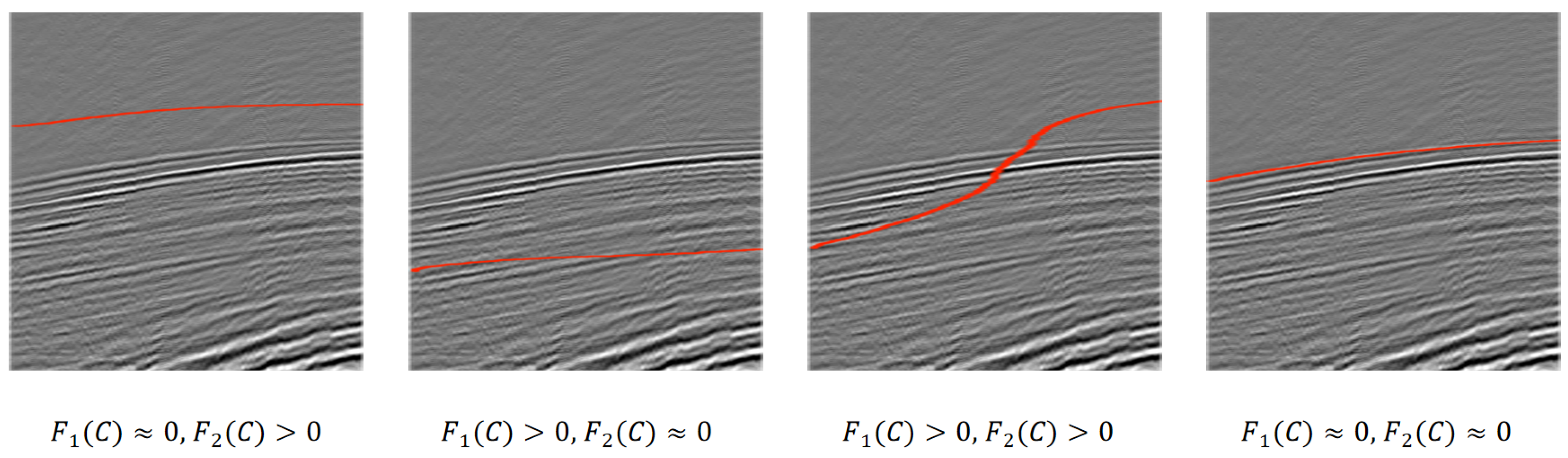
We can explain this by a seismic example in Figure 1. When the curve C is positioned above the FB curve, we observe that is approximately zero, while is positive. Conversely, when the curve C lies below the FB curve, becomes positive and approaches zero. If the curve C oscillates between being above and below the FB curve, both and are positive. Finally, when the fitting energy reaches its minimum, this indicates that the curve C perfectly matches the FB curve.
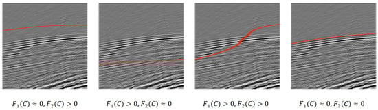
Figure 1.
This figure illustrates the variation of the proposed energy function with different positions of curve C.
In fact, only this fitting energy is not enough for our model. According to some prior knowledge of signal first breaks, the FB curve should be smooth to some extent. There are many ways to describe the smoothness of the curve. In our work, to simplify the final PDE form of the model, we choose the length of the curve. In fact, the curve length is used to represent continuity, as it directly measures the smoothness of the curve, favoring shorter and simpler boundaries. Additionally, its mathematical formulation is compact and well suited for numerical computation in the level set framework, ensuring efficient optimization.
Then, we can obtain the objective functional :
where , , are fixed parameters.
2.1. Unsupervised Method
2.1.1. Theory
Without using any labeled data, we can consider directly optimizing Equation (2) by the level-set method [20], which is a computational technique designed to monitor and analyze the dynamic changes in interfaces and shapes over time. It represents curves or surfaces in an implicit manner, where the interface characterized as the zero level-set of a higher-dimensional function, often referred to as the level-set function, denoted by . The curve or surface evolves over time by solving a partial differential equation (PDE) based on . The method’s robustness, flexibility, and mathematical elegance make it a powerful tool in various scientific and engineering fields. We focus on the optimization problem below:
is described as the zero level-set of a Lipschitz function , which satisfies
After that, we replace C by function . To express the terms in the energy F, we need to use the function H and , defined by
In this way, we next rewrite in the following form:
When we hold fixed and minimize the energy with respect to the constants and , they are in fact given by
In order to compute the associated Euler–Lagrange equation for , we need slightly regularized forms of H and . We use and as , and let be any regularization of H and . Then, to minimize with fixing and , we can derive the corresponding Euler–Lagrange equation for . By introducing an artificial time parameter , we have
Figure 2 illustrates the methodology of the proposed method. We initialize the level-set function , where the red curve represents the region where the function equals zero, i.e., the zero level-set. By solving the EL equation, undergoes multiple iterations until it stabilizes. The resulting zero level-set represents the desired first-break curve.
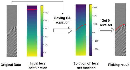
Figure 2.
Basic schematic diagram for the unsupervised algorithm. The red line refers to the 0 level-set curve.
2.1.2. Numerical Approximation and Algorithm
To obtain the numerical approximation of the model, first we need to find regularization of H by functions. There are several choices, and we choose to use a common one defined by
and is its derivative:
According to the analysis in [19], this choice typically leads to a global minimizer, regardless of the initial curve’s position, and enables the automatic detection of interior contours.
In order to discretize (5), a finite differences implicit scheme is needed. Let h represent the spatial step and the time step, with grid points for . Denote as the approximation of , with and . We adopt the discretization method in [19], which computes by the following algorithms:
An iterative method to solve this linear system is needed. Finally, we can give a framework to deal with the first-break picking problem with the initial seismic data.
- Algorithm Steps for picking FB:
- 1.
- Transform the original seismic image to energy-based image .
- 2.
- Initialize .
- 3.
- Calculate and . Use 6 to get by
- 4.
- Use to get the 0 level set, i.e., the FB curve.
- 5.
- Verify whether the FB curve is stationary. If not, increase n by 1 and repeat from step 3.
2.2. Supervised Method
2.2.1. Motivation
In recent years, first-break picking models using deep learning have been widely applied. In fact, when sufficient labeled data are available, a data-driven supervised semantic segmentation model can significantly outperform unsupervised models because the latter cannot utilize the information of the labeled data. It is well understood that deep learning-based models try to obtain the optimal solutions of the parameters by minimizing the empirical risk as expressed in the following equation:
where represents the empirical risk, represents the parameters of the deep learning model, represents the loss function, represents the deep model, and denote the input data and ground truth, respectively. In binary semantic segmentation tasks, some widely employed loss functions are Binary Cross Entropy (BCE), Dice Loss [21], and Focal Loss [22]. The commonly used Dice Loss can be expressed as follow:
where p denotes the output probability of the semantic segmentation model.
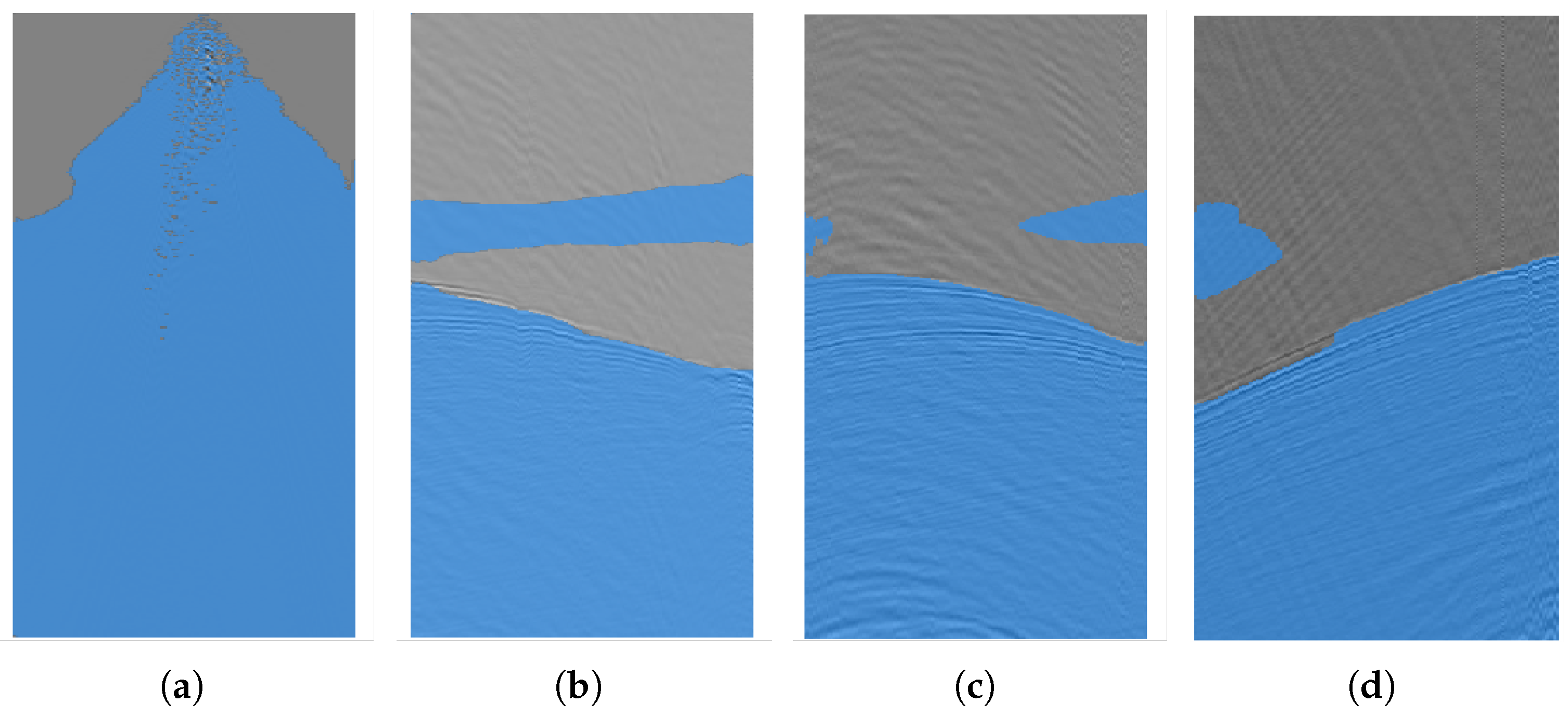
Given that deep semantic segmentation models achieve the pixel-level segmentation, the employed loss functions often exhibit certain limitations when applied to first-break picking task. This task in 2D seismic data fundamentally involves identifying the target curve on the image that accurately segments each trace into two distinct parts: pre-arrival and post-arrival. However, when testing a trained deep semantic segmentation model on a test set, it is common to encounter situations where the generated mask fails to produce a clearly defined segmentation curve. Figure 3 shows some result masks generated by a trained deep semantic segmentation model.
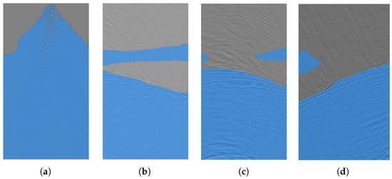
Figure 3.
Mask results generated by a trained U-Net model on four seismic data images. (a) This mask contains many pixels that are classified as non-FB after the first-arrival time, which is clearly an error. (b–d) Masks in (b), (c) and (d) all exhibit the issue of misclassifying some pixels before FB as FB, even though clear FB curves can be identified in the masks.
As seen from the result masks in Figure 3, the model is difficult to generate a suitable first-arrival time which meets the required conditions on these two test data. This difficulty arises because the model has not adequately learned the specific characteristics of the first-arrival picking. The main reason is that the loss function used in semantic segmentation networks is primarily intended for pixel-level segmentation and does not take into account the curve information inherent in the first-arrival time within the image.
2.2.2. Curve Loss Function for Deep Supervised Methods
In the previously discussed unsupervised method, we iteratively optimize to identify the first arrivals. The goal function (2) or (4) in this method can be divided into two components: a curve constraint part and a region constraint part. If we replace the fixed energy function in the second part (region constraint) of Equation (4) with p, we can observe that this component closely resembles the loss function used in supervised learning mode. Next, we try to design the curve constraint component of the supervised semantic segmentation loss function. Since the output mask is generated by applying a binary threshold to the output probability p, we can regard p as the 0.5 level-set for the target curve to some extent. We can then use certain properties of the target curve to reconstruct a curve loss function. Specifically, we consider , which is the gradient of the level-set function. We know that the direction of this gradient corresponds to the normal vector of the target curve, while the magnitude represents the rate of change of the curve in the normal direction. In the discrete case, we use differences in the two directions to approximate the gradient. The specific meaning of the differences can be illustrated by Figure 4.
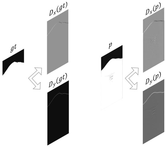
Figure 4.
A specific example of seismic data, where represents the ground truth mask and p represents the output probability of a model for this sample. Differences in both directions are computed for both and p.
From Figure 4, we can clearly observe that differences and effectively discover and actually express the characteristics of the target first-break curve. Based on this observation, we define the following curve loss:
where and , M and N denote the size of the input 2D seismic data. By combining the resulting with a basic semantic segmentation loss, we can get a loss function :
We use this combined loss function in the supervised learning mode for first-break picking problems.
3. Experiments for the Unsupervised Method
3.1. General Results
We first specifically implement the unsupervised algorithm presented in Section 2.1.2. For convenience, we will refer to the active contour method we propose as AC. In Step 1, transforming the original seismic image has several methods, an effective way in experiments is to use the absolute value of the image, i.e., . For Step 2, we always choose a straight line on top of the image , and initialize by the distance to the straight line. In Step 5, obtaining the 0 level-set by in practice is actually finding the value in the discrete . To address the first arrivals, it is necessary to identify the pick for every single trace; thus a reasonable way is to use the minimum absolute value for each trace, then we have
The FB curve we obtain in this step is actually a sequence of length M representing the 0 level-set of . When the sequence is stationary(practically, we think it is stationary if there are under 50 points changes), we can obtain the final pick for the original seismic image.
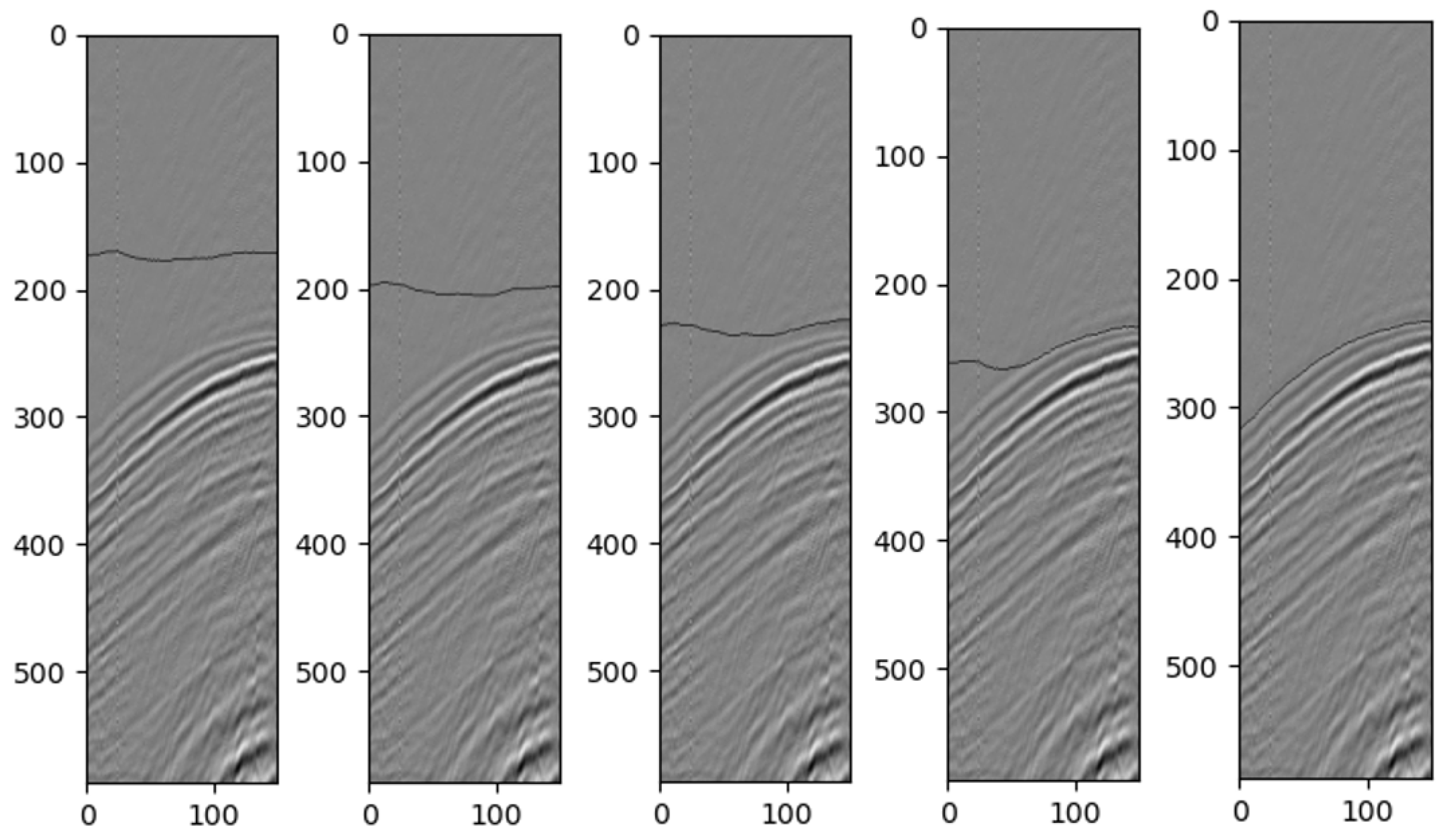
We use the real-world seismic data as examples for testing the level-set method. In the experiments, we choose , and . For the initial straight line, we choose . Figure 5 shows the curve iterative process in grayscale on a real seismic image. We cut 150 traces and the time samples for each trace are 600 (600 is the number we test here, and the real time-step number in the data is 876). From the figure, we can easily see the effectiveness of our method. In fact, except for the choice, the values for the other parameters are selected to be of big space. The detailed parameter selections are discussed in Section 4 part A. This also shows the robustness of the algorithm.
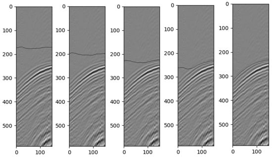
Figure 5.
Zero level-set curve changes in the grayscale image of the seismic data for every 400 time steps.
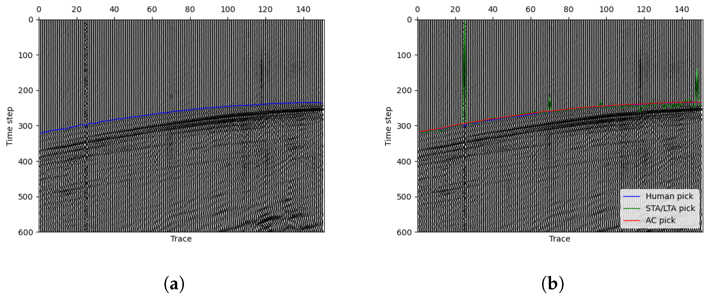
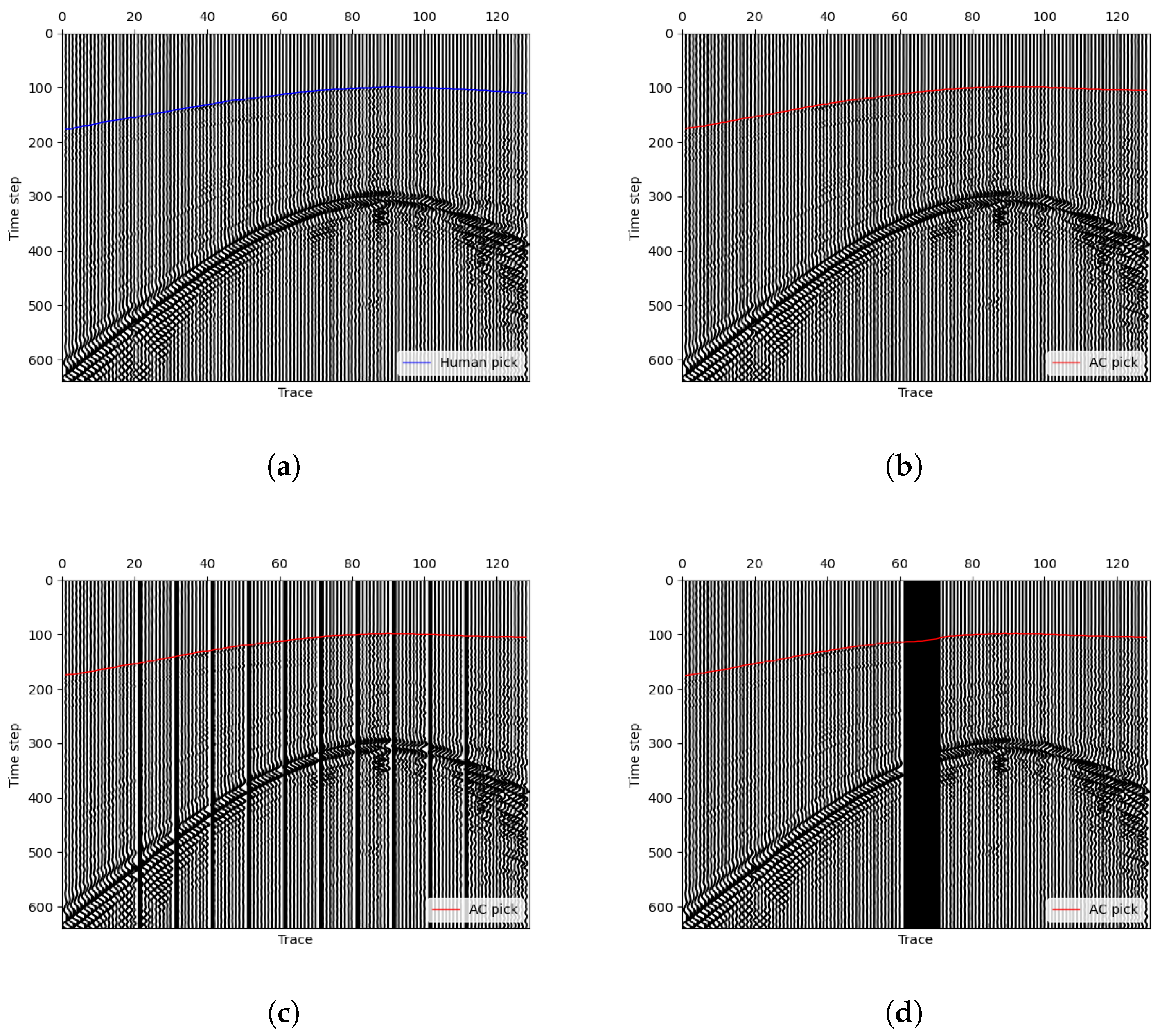
Instead of grayscale images, we often use wiggle image that can show the variation in wavelength in exploration geophysics. Figure 6a displays the used seismic data. The blue line represents the manual picking. In order to evaluate the performance of the proposed approach, we use the widely used standard STA/LTA method implemented in ObsPy to make a comparison. The STA/LTA algorithm detects seismic events by comparing the ratio of a short-term average (STA) to a long-term average (LTA) of signal amplitudes. A high STA/LTA ratio indicates a potential event, making this simple and efficient technique essential in real-time seismic detection. After testing in the seismic image, we choose STA = 10 and LTA = 100 with trigger threshold =4.5 to get the best result with the STA/LTA method. As shown in Figure 6b, the green curve shows the picking result made by the STA/LTA algorithm and the green one is the final stationary curve by our method. In the situation, our curve fits the manual label almost perfectly while the STA/LTA method makes many mistakes. The result analysis reveals that, as a training-free picking method, our approach demonstrates superior accuracy and noise resistance compared to the single-trace picking method STA/LTA. This is attributed to our method’s effective utilization of two-dimensional seismic signal information. Additionally, it is worth mentioning that if we take a closer look at the figure, it is easy to see that the 25th trace is full of noises and has no available signal. This happens frequently in actual seismic data recording, which is often affected by some accidental factors that lead to different kinds of noises. As a one-trace picking method, STA/LTA can not handle this situation. Since we have constrained the length (or smoothness) of the curve in the minimizing term, we can see that our method can deal with such one-trace noise very well. Based on this, we additionally conduct tests involving missing traces in 2D seismic images as depicted in Figure 7. To simulate missing traces, we transform the original single-trace data, setting the missing traces to the maximum value across the entire 2D dataset. We consider scenarios with 10 non-contiguous missing traces (Figure 7c) and 10 contiguous missing traces (Figure 7d). The results shown in the figure indicate the robust performance of our algorithm in handling both scenarios. In both cases, the picking accuracy within a range of two pixels (or time samples) exceeds 90%, and within five pixels, the picking rate reached 100%.
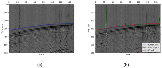
Figure 6.
Wiggle figures showing the seismic data and picking results. (a) The blue line shows the manual picking results. (b) The green line shows the STA/LTA method picking results, and the red line shows the results of our method.
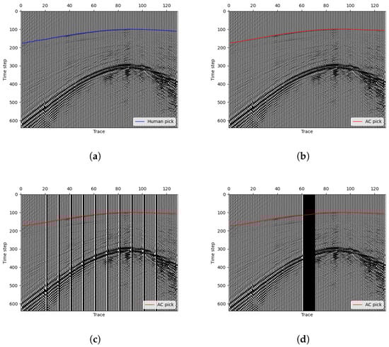
Figure 7.
Tests involving missing traces in 2D seismic data. (a,b) Original data with manual picking and our AC picking. (c) Our AC picking with 10 non-contiguous missing traces in the original data, and (d) AC picking with 10 contiguous missing traces.
3.2. Human Interaction
In order to find a better first-break for various different real-world data, human assistance is important. In fact, none of all the automatic first-break picking methods can give a perfect result for all different kinds of situations. The human assistance is indispensable for commercial companies to perform the first-break picking work. A well trained deep learning model can handle a large part of easy first-break picking problems; however, as shown in experiment part, the model still makes many mistakes in some situations due to different kinds of noise and geological conditions. Just like all the other picking methods, the active contour method we propose cannot solve all the picking problems either. When a machine learning-based model cannot accurately pick some first breaks, the general ways are enlarging training datasets, retraining models or fine tuning, which are time-consuming and often less effective for special geology situations. Thanks to the characteristics of the active contour model, when our algorithm performs poorly in picking some seismic images, there are many ways to enhance the picking results immediately by human interaction. Our proposed methods offer three approaches to enhance the picking quality using simple manual interactions. First, experts can quickly modify the model parameters to adjust the picking results. Second, a target region can be manually selected to achieve more precise picking outcomes. Third, experts can specify a fixed picking moment on the data, enabling the regeneration of a more optimal picking result across the entire seismic image. The subsequent sections offer a detailed explanation of the three methods.
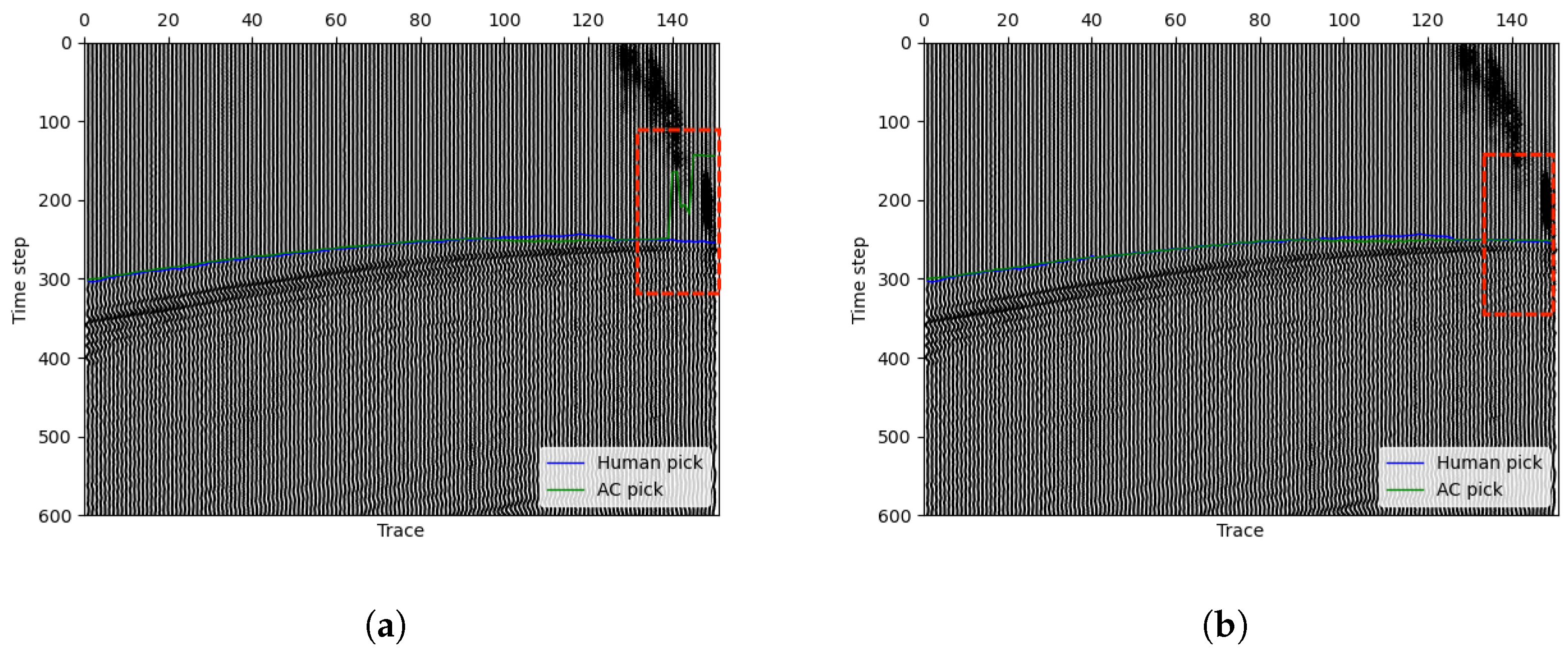
3.2.1. Parameters Selection
The unsupervised active contour model is not based on the learning method. Different parameters selections can give different picking results for one seismic image. A good parameter selection can give a good picking result. Comparing with deep learning-based methods, the model of ours is more transparent and interpretable. The parameters in our method always have a clear meaning, and a human user can easily obtain better picking results by changing the parameters. For example, the value of parameter reflects the continuity of the 0 level-set curve to some extent. As observed in Equation (2), is a parameter that penalizes the length of the target curve. To some extent, a larger value of indicates a stronger preference for a more continuous and smoother target curve, whereas a smaller suggests weaker requirements for the continuity of the target curve. Figure 8 gives an example for changing parameter . In this situation, the last few traces in the seismic data are greatly affected by noises. When we use the general parameter choice, the picking results are shown in Figure 8a, where the last few arrivals cannot be picked correctly. By increasing value to 60, which means increasing the continuity of the curve, we can obtain a better pick as shown in Figure 8b. For parameters and , they control the fitting of the target (after FB) and background (before FB) regions, respectively. Typically, a balanced setting works well, but adjustments can be made based on the seismic image. For instance, increase if the target region is challenging to capture or if the background has significant noise. These parameters are often fine-tuned experimentally to achieve optimal segmentation. The general parameter selections are shown in Table 1.
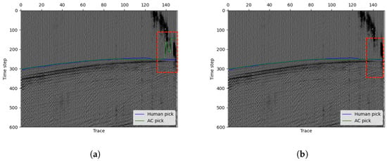
Figure 8.
Different choices affect the picking results of our method. (a) (b) . As seen from the picking within the red box, after using the modified parameters, the picking accuracy significantly improves due to the smoother FB curve.

Table 1.
General parameters chosen in our model.
3.2.2. Region Selection
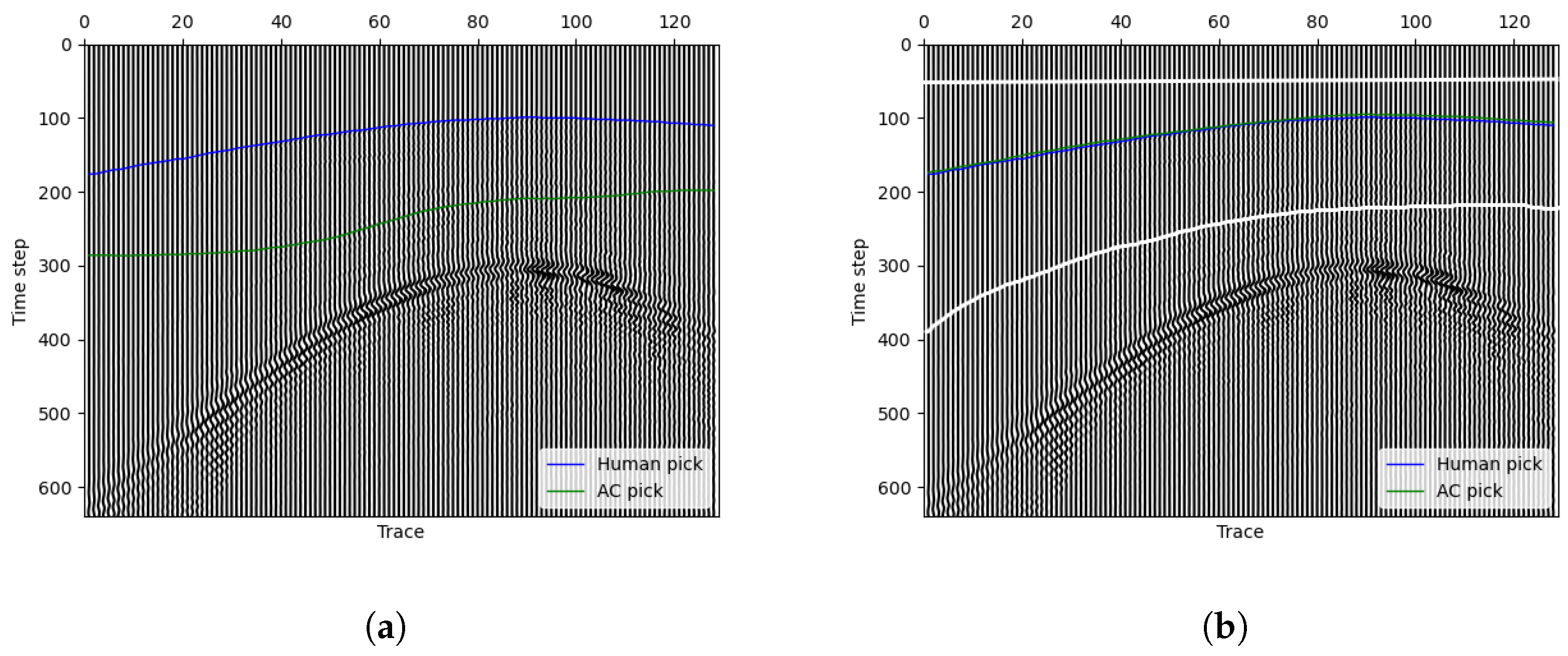
When employing image processing-based deep learning models for first arrival picking, it is essential to use a standardized image size when cropping images from the original seismic data. In contrast, the active contour model has the capability to identify first arrivals for any connected region (totally different from padding in deep learning methods), and we have implemented this functionality. In many situations, strong signals far from the first arrivals significantly impact the accuracy of the picking results. For many picking methods, strong signals far away after first arrivals often invalidate the method. Our method provides an approach for the human user to choose the picking region for better results. Here is an example for different region choices in our method. Figure 9a shows a situation where our method gives a picking result far away after the manual pick. If the signals are too strong far away from the arrivals, after data normalization, the signal change near the first-break will fade away. As it is easy for the naked eye to discern the regions with relatively high energy after the first arrival, we can manually draw a region (white lines in Figure 9b) to exclude these parts that might disturb the model. Our model yields a highly satisfactory first arrival picking result in this region as depicted in Figure 9b.
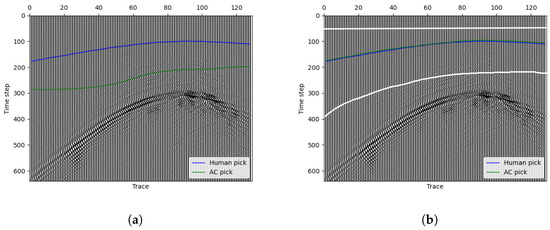
Figure 9.
Different region choice affects the picking results. (a) Whole region, (b) region choose by hand (between the upper and lower white lines).
3.2.3. Fix Points
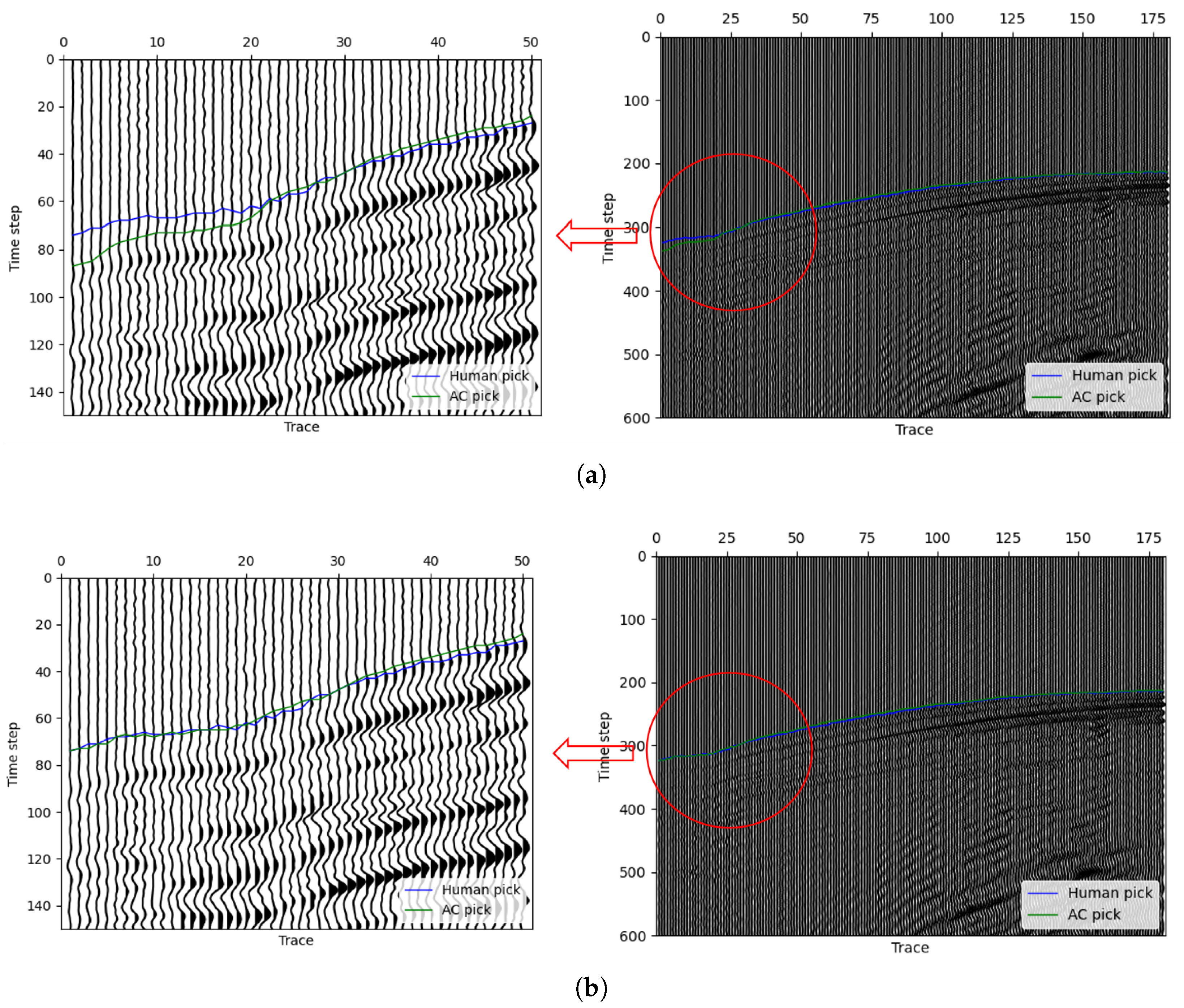
In our method, we can give some traces in the seismic data a fixed first-break and ensure that the first-break of these traces remain unchanged throughout the steps. In implementation, we reset in step 4 and make sure the FB picking of specific traces remain the same. As a result, the error between our prediction and manual pick moves in a good direction. Figure 10a left shows a situation where our model picking has obvious differences in a successive part of the first few traces. At the first 25 traces of the data, the manual picking label leaves an obvious distance of our picking curve, and the curve in the other traces perform very well. After we enlarge the first 50 traces, image shown in Figure 10a right, we can find that the signal intensity of the first 25 traces is weaker than the other. Then, by our method, the curve is finally stopped lower than the manual pick. Actually, if we only concern ourselves with the first 25 traces and try to find their first-break, it is almost an impossible task. After we consult some experts in related fields, we know that they often use the strong signals FB as reference for the weak signal FB. Therefore, algorithms like our method can hardly do the same thing in this situation as an expert. However, by fixing several traces, this problem can be solved to some extent. Figure 10b shows the picking results after fixing 1 trace in the first 25 traces, and the resultant picking is almost perfect in this situation. This experiment shows the effectiveness of our method with human assistance. In the real-world working situation, an expert can first use our method to obtain an approximately accurate first-break pick, and then by adjusting some results in a few traces, the algorithm will give a better solution. In addition, the algorithm with fixing points will cost smaller iteration steps and less time. This will greatly improve the work efficiency and quality.
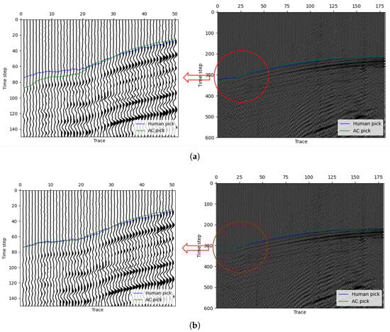
Figure 10.
An example demonstrating the use of fix-points method to improve the accuracy of first-break picking. (a) Picking results without fixed points, where the picking times within the red circle show a noticeable difference from the manually picked times. (b) Picking results after fixing a single trace, where the picking accuracy within the red circle significantly improves, reaching the level of manual picking.
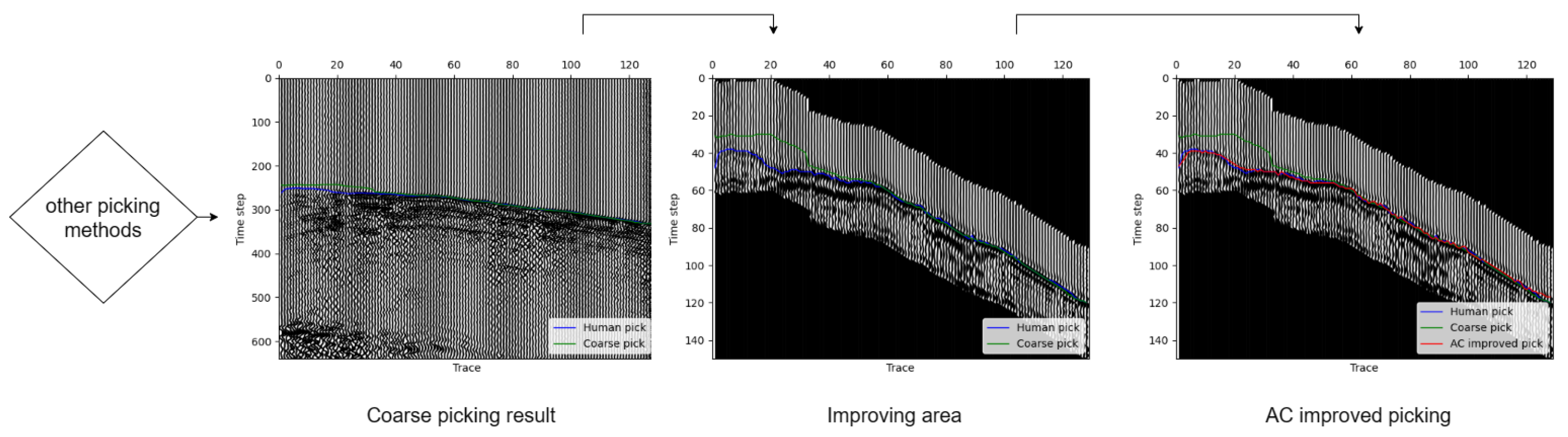
3.3. Improving Picking Results of Other Methods
The proposed picking model exhibits certain limitations when dealing with intricate scenarios. Due to its simplistic assumptions regarding seismic data, it frequently falters in situations characterized by complex noise patterns. While deep learning models trained on extensive datasets often showcase robust noise resistance, their precision in local picking may fall short. Consequently, a natural consideration involves leveraging a deep learning-based model to learn an approximate initial wave position. Around this position, a small contiguous region is generated. After data processing, our previously introduced region selection approach is reapplied for refined local picking, enhancing overall accuracy. The workflow for improving the picking performance with our method is depicted in Figure 11. We will demonstrate the effectiveness of our approach in improving picking accuracy through experimentation.
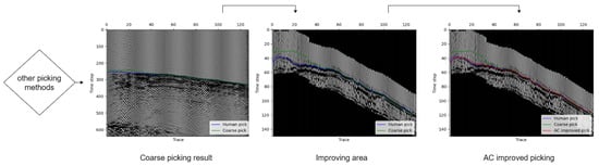
Figure 11.
The process of improving the picking results with our proposed method.
Unlike many studies that rely on synthetic datasets, we use only real seismic exploration data, ensuring a more reliable validation of the method’s applicability in real-world conditions. The land shot gathers used in our study are supplied by BGP Inc., Zhuozhou, China, a subsidiary of China National Petroleum Corporation. The dataset includes hundreds of shots, with each shot comprising more than 8000 spatial traces and numerous time samples. To optimize the deep neural network’s ability to learn from the seismic data, we segment the original data into smaller slices, each containing 128 spatial traces and 640 time samples. For testing, we select 921 image slices. Importantly, these slices are never involved in the training process, ensuring that the test set serves as a fair evaluation of all model algorithms. For the training process, we created three groups of datasets of varying sizes of seismic image, extracted from 5, 10, 20, and 160 shots. By training models on datasets of different sizes, we evaluate the generalization picking performance of the models for other regions. This approach helps assess the robustness of the models when fewer training samples are available. The UNet we use has a Resnext 52 encoder pretrained on ImageNet and it demonstrates superior performance in our other deep learning-based model experiments. Detailed information about the UNet we use is displayed in Table 2.
Table 2.
Information about the utilized UNet.
Using the obtained UNet picking results on test datasets as a reference, we employ our proposed active contour model and obtain a new picking with the method in Section 3.2 part B. The experimental picking accuracy are presented in Table 3.
Table 3.
Test picking results for the UNet trained with different training datasets. accuracy stands for the proportion of the traces picking error less than N time samples in all test traces.
The columns in the table respectively represent the proportion of the model’s first-break picking results differing from the manual picking results by 1, 2, 5, and 10 time samples, normalized by the total number of traces. The first three rows of the table represent the picking performance of three UNet models trained on 5, 10, and 20 shots respectively. The fourth row indicates the picking accuracy of a UNet model trained on five shots using our AC method for enhancement. From the table, it is evident that the unsupervised model, after enhancing the insufficiently trained UNet, outperforms the picking results of UNet model trained with twice the training data. Moreover, its performance is comparable to that of the almost fully trained UNet model with 20-shot training data. This suggests that our approach significantly improves the first-arrival picking accuracy for insufficiently trained supervised models.
4. Experimental Results for the Deep Supervised Methods
In this section, we replace the loss function in the deep semantic segmentation model with the proposed loss function (7). We train the model under the same conditions, followed by testing on the same test dataset. In the first-break picking problem, the derivative in the time sampling direction is significantly more important than that in the trace direction, as we need a precise boundary line on each trace. Therefore, we typically set to be smaller than . In practice, considering the relative magnitude with respect to the base loss, we set to 1 and to 10.
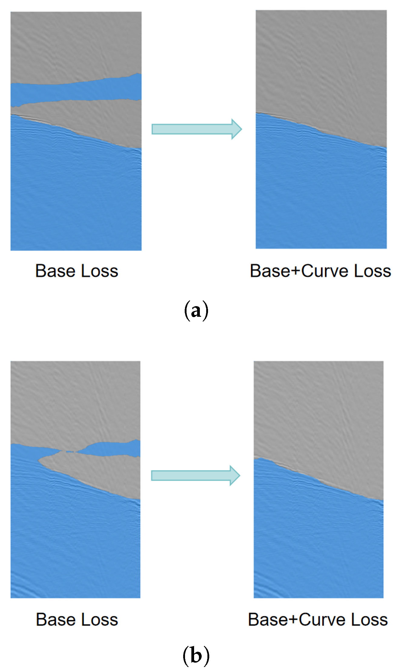
Figure 12 below shows a comparison of masks generated on test seismic data by two models: one trained using only the Base Loss and the other trained using the proposed loss, with all other training conditions kept the same. It is evident that the model trained with our proposed loss function generates masks with significantly reduced interference and more closely aligns with the requirements of the first-arrival picking problem. Additionally, to validate the broad applicability of our loss function, we train multiple deep semantic segmentation models using different base losses, different dataset sizes, and different model architectures. We evaluate these models using both the base loss and our combined loss function. The experimental results presented in Table 4 illustrate that deep learning models trained using our proposed loss function achieve substantial advancements in the first-break picking task.

Figure 12.
Masks obtained from a trained deep learning model with and without the proposed curve loss. (a), (b) present two examples, where the picking masks show significant improvement after training with our loss function.
Table 4.
Experimental results for the deep semantic segmentation models trained with and without FB Loss testing on test seismic data. accuracy stands for the proportion of traces picking error less than N time samples in all test traces.
Our experiments demonstrate that using this loss function allows deep learning models to learn the characteristics of the first-break picking problem more effectively.
5. Conclusions and Remarks
The task of identifying the first arrivals in 2D seismic waveform data can be framed as an image segmentation task. In this work, we propose a method which optimizes the geometric properties of the target curve for first-break picking, which can be successfully applied in both unsupervised and supervised learning frameworks. The proposed unsupervised model accurately picks first arrivals in 2D seismic data and outperforms traditional methods. This method does not need any training in different environments and enables accurate first-break picking without any supervised learning. We develop several human interaction approaches that can substantially improve the picking accuracy, which allows experts to efficiently and accurately label first arrivals in seismic data. We also design a post-processing method which can be used to enhance the picking of other methods by using the unsupervised approach. For supervised deep learning methods, we introduce a curve loss function, which significantly improves the performance of supervised models in first-break picking tasks through extensive experiments.
Our methods still have points that need improvement. The proposed unsupervised model has a relatively slower iteration speed compared to well-trained deep learning models ignoring the training time. Algorithm acceleration stands out as a potential future direction for our unsupervised active contour methodology. If our algorithm can achieve a faster picking process, it becomes feasible to iteratively apply this algorithm multiple times, potentially leading to a significant improvement in automatic picking. We aim to explore a more integrated approach in the future that combines deep learning models with our current method, beyond merely modifying the loss function. We aim to introduce a new supervised model by adjusting the architecture so that it can leverage the supervised information, while also utilizing the unsupervised picking capabilities of the active contour model. This approach is intended to achieve more accurate and faster first-break picking, while also being capable of handling a wider range of noise types. Additionally, it should be noted that seismic data collected in real-world scenarios are often in 3D format due to the arrangement of signal receivers in a 2D manner on the surface. In practice, 2D seismic images are typically generated by extracting sections of the 3D data. The extension of the active contour model from 2D to 3D is theoretically straightforward. However, due to limitations in computational efficiency and the impact of noise, directly applying the same parameters in the 3D model does not yield satisfactory picking results. In the future, we aim to address this issue and incorporate 3D data into the model, as 3D data contain a greater amount of information compared to the clipped 2D images.
Author Contributions
Conceptualization, J.M. and Z.W.; methodology, Z.W.; software, Z.W.; validation, Z.W.; formal analysis, Z.W.; investigation, Z.W.; writing—original draft preparation, Z.W.; writing—review and editing, J.M. and Z.W.; visualization, Z.W.; supervision, J.M.; project administration, J.M.; funding acquisition, J.M. All authors have read and agreed to the published version of the manuscript.
Funding
This research was funded by the Natural Science Foundation of China under grant 62071171.
Data Availability Statement
Due to privacy restrictions, the labeled seismic data in our work used for testing and training cannot be shared.
Acknowledgments
We acknowledge the support of the High-performance Computing Platform at Peking University and express our gratitude to BGP Inc. (Zhuozhou, China), China National Petroleum Corporation, for supplying the privately labeled seismic data.
Conflicts of Interest
The authors declare no conflicts of interest.
References
- Akram, J.; Eaton, D.W. A review and appraisal of arrival-time picking methods for downhole microseismic data. Geophysics 2016, 81, KS71–KS91. [Google Scholar] [CrossRef]
- Allen, R.V. Automatic earthquake recognition and timing from single traces. Bull. Seismol. Soc. Am. 1978, 68, 1521–1532. [Google Scholar] [CrossRef]
- McCormack, M.D.; Zaucha, D.E.; Dushek, D.W. First-break refraction event picking and seismic data trace editing using neural networks. Geophysics 1993, 58, 67–78. [Google Scholar] [CrossRef]
- Maity, D.; Aminzadeh, F.; Karrenbach, M. Novel hybrid artificial neural network based autopicking workflow for passive seismic data. Geophys. Prospect. 2014, 62, 834–847. [Google Scholar] [CrossRef]
- Mousavi, S.M.; Beroza, G.C. Deep-learning seismology. Science 2022, 377, eabm4470. [Google Scholar] [CrossRef] [PubMed]
- Guo, C.; Zhu, T.; Gao, Y.; Wu, S.; Sun, J. AEnet: Automatic Picking of P-Wave First Arrivals Using Deep Learning. IEEE Trans. Geosci. Remote Sens. 2021, 59, 5293–5303. [Google Scholar] [CrossRef]
- Zhu, W.; Beroza, G.C. PhaseNet: A deep-neural-network-based seismic arrival-time picking method. Geophys. J. Int. 2019, 216, 261–273. [Google Scholar] [CrossRef]
- Zheng, J.; Lu, J.; Peng, S.; Jiang, T. An automatic microseismic or acoustic emission arrival identification scheme with deep recurrent neural networks. Geophys. J. Int. 2018, 212, 1389–1397. [Google Scholar] [CrossRef]
- Yuan, S.; Liu, J.; Wang, S.; Wang, T.; Shi, P. Seismic Waveform Classification and First-Break Picking Using Convolution Neural Networks. IEEE Geosci. Remote Sens. Lett. 2018, 15, 272–276. [Google Scholar] [CrossRef]
- Hollander, Y.; Merouane, A.; Yilmaz, O. Using a deep convolutional neural network to enhance the accuracy of first-break picking. In SEG Technical Program Expanded Abstracts 2018; SEG: Houston, TX, USA, 2018; pp. 4628–4632. [Google Scholar] [CrossRef]
- Duan, X.; Zhang, J.; Liu, Z.; Liu, S.; Chen, Z.; Li, W. Integrating seismic first-break picking methods with a machine learning approach. In SEG Technical Program Expanded Abstracts 2018; SEG: Houston, TX, USA, 2018; pp. 2186–2190. [Google Scholar] [CrossRef]
- Hu, L.; Zheng, X.; Duan, Y.; Yan, X.; Hu, Y.; Zhang, X. First-arrival picking with a U-net convolutional network. Geophysics 2019, 84, U45–U57. [Google Scholar] [CrossRef]
- Ronneberger, O.; Fischer, P.; Brox, T. U-Net: Convolutional Networks for Biomedical Image Segmentation. arXiv 2015. Available online: http://arxiv.org/abs/1505.04597 (accessed on 28 October 2024).
- Yuan, P.; Wang, S.; Hu, W.; Wu, X.; Chen, J.; Nguyen, H.V. A robust first-arrival picking workflow using convolutional and recurrent neural networks. Geophysics 2020, 85, U109–U119. [Google Scholar] [CrossRef]
- Mousavi, S.M.; Ellsworth, W.L.; Zhu, W.; Chuang, L.Y.; Beroza, G.C. Earthquake transformer—An attentive deep-learning model for simultaneous earthquake detection and phase picking. Nat. Commun. 2020, 11, 3952. [Google Scholar] [CrossRef]
- Tsai, K.C.; Hu, W.; Wu, X.; Chen, J.; Han, Z. Automatic First Arrival Picking via Deep Learning With Human Interactive Learning. IEEE Trans. Geosci. Remote Sens. 2020, 58, 1380–1391. [Google Scholar] [CrossRef]
- Yuan, S.Y.; Zhao, Y.; Xie, T.; Qi, J.; Wang, S.X. SegNet-based first-break picking via seismic waveform classification directly from shot gathers with sparsely distributed traces. Pet. Sci. 2022, 19, 162–179. [Google Scholar] [CrossRef]
- Jiang, P.; Deng, F.; Wang, X.; Shuai, P.; Luo, W.; Tang, Y. Seismic First Break Picking Through Swin Transformer Feature Extraction. IEEE Geosci. Remote Sens. Lett. 2023, 20, 1–5. [Google Scholar] [CrossRef]
- Chan, T.; Vese, L. Active contours without edges. IEEE Trans. Image Process. 2001, 10, 266–277. [Google Scholar] [CrossRef] [PubMed]
- Osher, S.; Sethian, J.A. Fronts propagating with curvature-dependent speed: Algorithms based on Hamilton-Jacobi formulations. J. Comput. Phys. 1988, 79, 12–49. [Google Scholar] [CrossRef]
- Sudre, C.H.; Li, W.; Vercauteren, T.; Ourselin, S.; Jorge Cardoso, M. Generalised dice overlap as a deep learning loss function for highly unbalanced segmentations. In Proceedings of the Deep Learning in Medical Image Analysis and Multimodal Learning for Clinical Decision Support: Third International Workshop, DLMIA 2017, and 7th International Workshop, ML-CDS 2017, Held in Conjunction with MICCAI 2017, Québec City, QC, Canada, 14 September 2017; pp. 240–248. [Google Scholar]
- Lin, T.Y.; Goyal, P.; Girshick, R.; He, K.; Dollár, P. Focal loss for dense object detection. In Proceedings of the IEEE International Conference on Computer Vision, Honolulu, HI, USA, 21–26 July 2017; pp. 2980–2988. [Google Scholar]


Disclaimer/Publisher’s Note: The statements, opinions and data contained in all publications are solely those of the individual author(s) and contributor(s) and not of MDPI and/or the editor(s). MDPI and/or the editor(s) disclaim responsibility for any injury to people or property resulting from any ideas, methods, instructions or products referred to in the content. |
© 2025 by the authors. Licensee MDPI, Basel, Switzerland. This article is an open access article distributed under the terms and conditions of the Creative Commons Attribution (CC BY) license (https://creativecommons.org/licenses/by/4.0/).