Abstract
We explore a new approach for the parsimonious, generalizable, efficient, and potentially automatable characterization of spectral diversity of sparse targets in spectroscopic imagery. The approach focuses on pixels which are not well modeled by linear subpixel mixing of the Substrate, Vegetation and Dark (S, V, and D) endmember spectra which dominate spectral variance for most of Earth’s land surface. We illustrate the approach using AVIRIS-3 imagery of anthropogenic surfaces (primarily hydrocarbon extraction infrastructure) embedded in a background of Arctic tundra near Prudhoe Bay, Alaska. Computational experiments further explore sensitivity to spatial and spectral resolution. Analysis involves two stages: first, computing the mixture residual of a generalized linear spectral mixture model; and second, nonlinear dimensionality reduction via manifold learning. Anthropogenic targets and lakeshore sediments are successfully isolated from the Arctic tundra background. Dependence on spatial resolution is observed, with substantial degradation of manifold topology as images are blurred from 5 m native ground sampling distance to simulated 30 m ground projected instantaneous field of view of a hypothetical spaceborne sensor. Degrading spectral resolution to mimicking the Sentinel-2A MultiSpectral Imager (MSI) also results in loss of information but is less severe than spatial blurring. These results inform spectroscopic characterization of sparse targets using spectroscopic images of varying spatial and spectral resolution.
1. Introduction
Recent years have seen the global archive of imaging spectroscopy data grow substantially in both quantity and quality. Plans for further expansion are underway in both private and public sectors. Extracting maximum value from the ongoing and projected influx of spectroscopic data will require new analytic approaches capable of mapping subtle spectroscopic reflectance signals which are not captured by multispectral imagers. The volume and velocity of planned global spectroscopic imaging constellations will require approaches which, in addition to being analytically powerful, are generalizable and computationally efficient.
Further, many of the features of interest, particularly those built by humans, can occur in a spatially distributed manner. The signatures of interest may be spatially clustered or may be heterogeneously distributed across an extensive background area. The implication of this spatial sparsity is that the vast majority of pixels are not of interest to such analyses. This observation of spatial sparsity could yield substantial gains in analysis efficiency, and thus global utility. But in order to do so, an approach must be capable of: (1) finding sparse targets with unknown spectral signatures, and (2) characterizing their spectral diversity, in a (3) generalizable, efficient way.
The first challenge can be framed in the context of target detection. Over the decades, a wide set of analytic tools has been developed to map sparse targets. Prominent in this toolkit are the Matched Filter [1,2] and its Mixture-Tuned variety [3]; subspace-based algorithms like Orthogonal Subspace Projection [4], and Anomaly Detectors like the RX algorithm [5]. Operational use cases for such algorithms are plentiful, perhaps most prominently including methane leak detection and monitoring, e.g., [6]. For a review of approaches to the target detection problem, see [7]. However, many of these approaches require prior information (e.g., reference spectra) about the expected target signature, while some problems offer minimal prior information about what the target materials might be, and/or must accommodate the potential for a heterogenous set of equally important potential reference materials.
Uncertain or variable target signatures lead to the second challenge: characterization of the diversity of unknown signatures in a scene (in which the set of spectral signatures of interest are not already known). A set of tools also exists for this purpose. Most prominent among these is the longstanding Principal Component Analysis [8], as well as Independent Component Analysis [9], the Maximum Noise Fraction transform [10] and the Pixel Purity Index [11]. In some instances, both target detection and characterization can be enhanced through spectral pre-treatment approaches like continuum removal [12] or smoothing filters (e.g., [13]). These algorithms have a wide range of computational costs and scene specificity, many of which are challenging to generalize to large study areas and/or data volumes.
The third challenge, efficient generalization, is key to algorithm scalability. Here, recent advances may offer an opportunity for improvement. Specifically, the recognition that the vast majority of variance (>99% pixels with <5% RMSE) in terrestrial spectra can be reasonably approximated as linear mixtures of soil, rock, and nonphotosynthetic vegetation Substrate (S), illuminated photosynthetic Vegetation (V), and Dark targets like shadow, water, and low albedo surfaces (D). This observation was recognized in decameter multispectral satellite imagery decades ago [14,15], generalized to spectroscopic [16,17,18] imagery, and confirmed with multiple multispectral sensors and image compilations [19,20,21,22] (with some notable exceptions like evaporite minerals, shallow aquatic targets, and cryosphere).
Here we explore an example workflow to characterize unknown sparse spectral diversity in imaging spectroscopy datasets. By leveraging the observed generality of the dominance of linear SVD mixtures in terrestrial images, this approach may be useful in both improving the generalizability and efficiency of existing algorithms and in developing new analytic approaches.
Our illustrative example focuses on mapping anthropogenic materials (the sparse target) in an Arctic tundra landscape (the dominant background). We use spectroscopic imagery from the novel AVIRIS-3 sensor to investigate the potential of a new approach, joint characterization of the spectral mixture residual, to (1) identify sparse spectroscopic targets and (2) characterize their spectral diversity in a (3) generalizable and computationally efficient way. In so doing, we ask the following questions:
- To what extent can misfit (both aggregate and wavelength-explicit residuals) of a generalized linear spectral mixture model provide additional information about spectral diversity of the built environment in Arctic tundra?
- How do readily identifiable spectral endmembers in high misfit pixels compare to those identified from full images?
- How do the spectral endmember signatures identified using the spectral mixture residual compare to results using reflectance alone?
- 2.
- How does characterization vary with spectral resolution?
- What, if any, target signatures are identified from AVIRIS-3 which are not present in simulated Sentinel-2?
- 3.
- How (if at all) do the answers to Questions 1 and 2 above vary with simulated coarsening spatial resolution?
- What, if any, signals are identified at 4 m resolution are and are not retained at the 30 m resolution of a potential future spaceborne imaging spectroscopy mission?
Question 1 investigates the potential for the new approach to identify and characterize spatially sparse spectroscopic targets, specifically focusing on endmember identification (Subquestion a) and diversity (Subquestion b). Question 2 focuses on the added value of spectroscopic versus multispectral information, highlighting the instances of information gain (as well as instances of similarity) in spectroscopic versus simulated multispectral observations. This question is central to showing utility for analyses working with multispectral data, as well as highlighting the new information which is present in spectroscopic imagery. Question 3 investigates the spatial resolution dependence of this result. Spatial resolution dependence is a critical factor for the use of spaceborne imaging spectroscopy data, which can be an order of magnitude (or more) spatially coarser than airborne imaging spectroscopy data. Taken together, answers to these questions present new information which may be useful to scientists considering implementing this new approach in their own work.
2. Materials and Methods
2.1. Study Area
The north slope of the Brooks Range in Alaska (Figure 1) hosts the Prudhoe Bay oil field. The Prudhoe Bay oil field is situated above the Arctic circle on continuous permafrost tundra, just north of the Brooks Range of mountains. This region is also home to diverse flora and fauna species, including caribou, polar bears, and musk oxen. It lies adjacent to the Arctic National Wildlife Refuge and critical ocean habitat areas. Prudhoe Bay was discovered to house oil in 1968 and began production in 1977. It currently produces over 19,013 barrels of crude oil per day. Prudhoe Bay is the largest oil field in the United States, covering 213,543 acres aboveground.
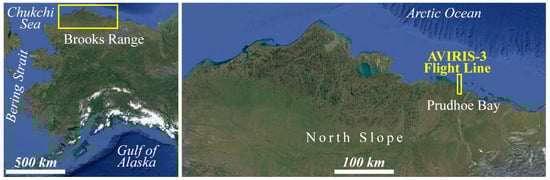
Figure 1.
Location. The Brooks Range runs over 1000 km from the Chukchi Sea, across northern Alaska, into the Yukon Territory. Its north slope, running to the Arctic Ocean, hosts the Prudhoe Bay Oil Field. Discovered on 12 March 1968 by ARCO and Exxon, Prudhoe Bay field is commonly recognized as the largest in North America. Estimates of original oil volume are 25 billion barrels. Production at Prudhoe Bay came onstream in the late 1970s and continues to present.
2.2. Methods
2.2.1. Data
Data used in this analysis were collected by the Airborne Visible/Infrared Imaging Spectrometer 3 (AVIRIS-3) sensor. AVIRIS-3, an optically fast F/1.8 Dyson imaging spectrometer, is the third of the AVIRIS spectrometer series [23]. AVIRIS uses the EMIT spectrometer design [24]. It is cryogenically cooled and makes observations of Earth-leaving radiance from 380 to 2500 nm with 7.4 nm spectral sampling. The spatial field of view is 39.5 degrees, discretized into 1240 swath samples with 0.56 milliradian sampling per sample. For more details about the AVIRIS-3 instrument, see [23].
This analysis relies on flight line AV320230806t205810, collected on 6 August 2023. Flight orientation was north to south. Flight altitude was approximately 7500 m. No clouds are visible in the image. Data were downloaded free-of-charge from the AVIRIS-3 data portal (https://popo.jpl.nasa.gov/mmgis-aviris/?mission=AVIRIS, accessed 1 October 2024) as Level-2A ISOFIT-corrected reflectance. ISOFIT [25] uses an Optimal Estimation (Bayesian) inversion strategy which produces simultaneous estimates of local aerosol and atmospheric water vapor constituents and wavelength-explicit uncertainties, as well as estimates of hemispherical-directional reflectance. ISOFIT code is open source and publicly available at https://github.com/isofit/isofit/ [Accessed 23 October 2024]. In addition to AVIRIS-3, ISOFIT is also used as the operational atmospheric correction for the EMIT mission [26].
Figure 2 shows a 1500-pixel spatial subset of the full flight line as both true color (left) and false color (right) composites. In accordance with study design, most of the study area is covered by the natural arctic tundra landscape comprised of a mosaic of permafrost and thermokarst lakes. Human disturbance associated with the network of hydrocarbon extraction infrastructure is dispersed across the landscape. Three 400 × 400 pixel subsets (yellow squares) were selected as representative samples of mixed permafrost + anthropogenic areas.
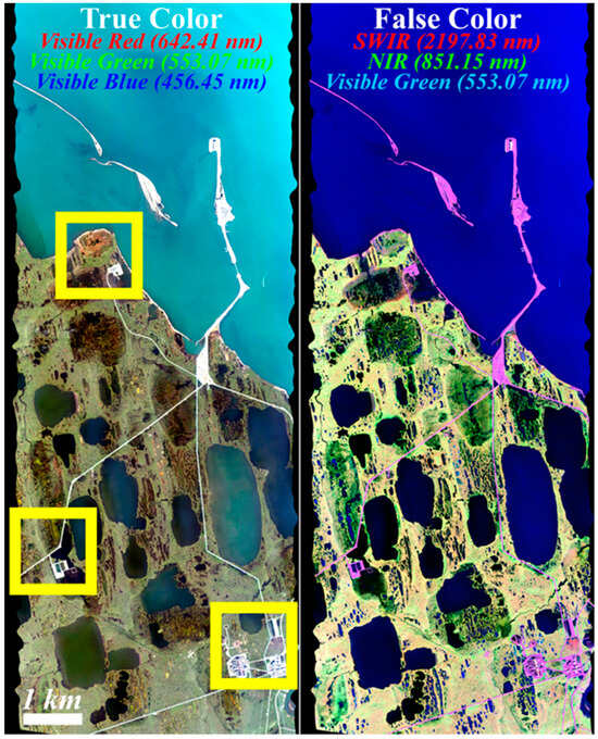
Figure 2.
AVIRIS-3 flight line overview. The first component of the analysis uses an example flight line (AV320230806t205810) acquired on 6 August 2023. These data were collected at approximately 4100 m (13,450 ft) flying in a north–south orientation. True color (left) and false color (right) images show Level-2A ISOFIT-corrected reflectance in north up orientation. A linear 2% stretch is applied to both images. Ground sampling distance is 4.1 m. Hydrocarbon extraction infrastructure is clearly visible amongst a typical north slope landscape mosaic of permafrost and thermokarst lakes. Yellow squares show the three 400 × 400 pixel subsets mosaiced and used for subsequent analysis.
Input data preparation focused on removing bad bands in which sensor noise and/or atmosphere absorption artifacts were observed. For this analysis, bands 1–10, 98–105, 127–150, 185–220, and 275–284 (corresponding to wavelengths 389.75 to 456.45 nm, 1112.21 to 1164.41 nm, 1328.41 to 1499.75 nm, 1760.12 to 2019.99 nm, and 2427.05 to 2493.48 nm) were flagged and excluded from analysis, resulting in retention of a total of 196 of 284 bands. Labeling of targets was not necessary for this analysis given the unsupervised nature of PCA and UMAP.
2.2.2. Analysis
The bulk of the methodology is designed to address Research Question 1 (To what extent can spectral mixture model misfit inform characterization of the built environment in arctic tundra landscapes). In order to address the added value (or lack thereof) of the spectral mixture residual for spectral characterization, we first approach the question of characterization of the reflectance data directly. We do so through the consideration of both high-variance and low-variance features using the conceptual framework of Joint Characterization [27]. Characterization of high variance features is conducted through Principal Component Analysis (PCA, [8]), and characterization of additional low-variance features is explored through Uniform Manifold Approximation and Projection (UMAP, [28]).
UMAP is an approach to nonlinear dimensionality reduction. Generally categorized as an example of Manifold Learning [29], UMAP follows previous approaches like t-SNE [30] and Locally Linear Embedding [31,32,33] in leveraging the connectivity structure of the data in high-dimensional feature space. UMAP specifically assumes the data can be modeled as high-dimensional observations distributed along a generative Riemannian manifold. UMAP seeks to learn this manifold and display it in a low-dimensional embedding space in such a way to faithfully preserve statistically local connectivity relations. Recently, UMAP has been increasingly used to visualize high dimensional data from fields as diverse as genomics [28], sonography [34], geochemistry [35], medical imaging [36], and more.
In this analysis, we used both 2D and 3D embedding spaces. Perhaps the most sensitive UMAP hyperparameter is the number of nearest neighbors (NN) used in the analysis. For this analysis, we explored a range of hyperparameter choices, settling on NN = 30, min_dist = 0.1, metric_choice = Euclidean, and n_dimensions = 2 or 3 for the final products. For more details about UMAP, the interested reader is directed towards [28]. UMAP is fully open source and available for download free-of-charge through the package ‘umap-learn’ available at https://umap-learn.readthedocs.io/en/latest/ [accessed 23 October 2024].
We also explore the application of the spectral mixture residual as a pre-treatment of the reflectance data before Joint Characterization. The spectral mixture residual [16] attempts to isolate low-variance (but high information) features by modeling and removing the broad land cover-driven mixing signal associated using a simple linear mixture model derived from generalized endmembers. Rather than seeking the optimal per-pixel mixture model fit, this approach instead treats misfit from the mixture model as a potential source of information, which then is used as the basis for subsequent characterization. This approach has proved useful for a wide range of datasets in imaging spectroscopy and multispectral imaging [16,17,37,38]. Mathematically, the spectral mixture residual can be computed as the wavelength-explicit residual of a linear spectral mixture model of the form:
where r is the pixelwise vector of surface reflectance, E is the matrix of endmember reflectance spectra, f is the vector of estimated endmember fractions, and ε is model misfit. For this study, we use the root-mean-square (L2) error norm, as well as an additional unit-sum constraint equation in which the sum of all fractions equals unity.
r = Ef + ε,
Computational experiments are used to address Research Questions 2 (impact of spatial resolution) and 3 (impact of spectral resolution). Spatial resolution is explored through convolution of the AVIRIS-3 reflectance mosaic using a low-pass Gaussian blurring kernel designed to simulate the point spread function of a hypothetical spaceborne imaging spectrometer with a 30 m Full Width Half Maximum (FWHM). Spectral resolution is explored through convolution of pixel spectra with the published spectral response function of the Sentinel-2A MultiSpectral Imager (MSI) [39].
All computations were performed on a standard 2020 13-inch MacBook Pro with a 2 GHz Quad-Core Intel i5 CPU, Intel Iris Plus Graphics 1536 MB graphics, 32 GB of 3733 MHz RAM, and 1 TB of solid-state storage. Computation time ranged from <15 s for Principal Component Analysis of the masked dataset to 96 min (and ~60 GB of RAM + SSD paging) for the largest UMAP embedding.
2.2.3. Workflow
The workflow for this analysis proceeds as follows:
- Evaluate spectroscopic diversity in reflectance data using PCA;
- Evaluate spectroscopic diversity in reflectance data using UMAP;
- Apply spectral mixture residual;
- Evaluate spectroscopic diversity in mixture residual data using PCA;
- Evaluate spectroscopic diversity in mixture residual data using UMAP;
- Map anthropogenic targets;
- Spatially blur to simulate point spread functions of coarser image data;
- Evaluate change in characterization and mapping to loss of spatial resolution;
- Spectrally convolve to mimic multispectral imaging sensors;
- Evaluate change in characterization and mapping to loss of spectral resolution.
Note that this workflow is designed for this demonstrative analysis and could easily be substantially shortened or refined for the purposes of a particular study application.
3. Results
3.1. Research Question 1: Informing Spectral Characterization with Mixture Model Residual
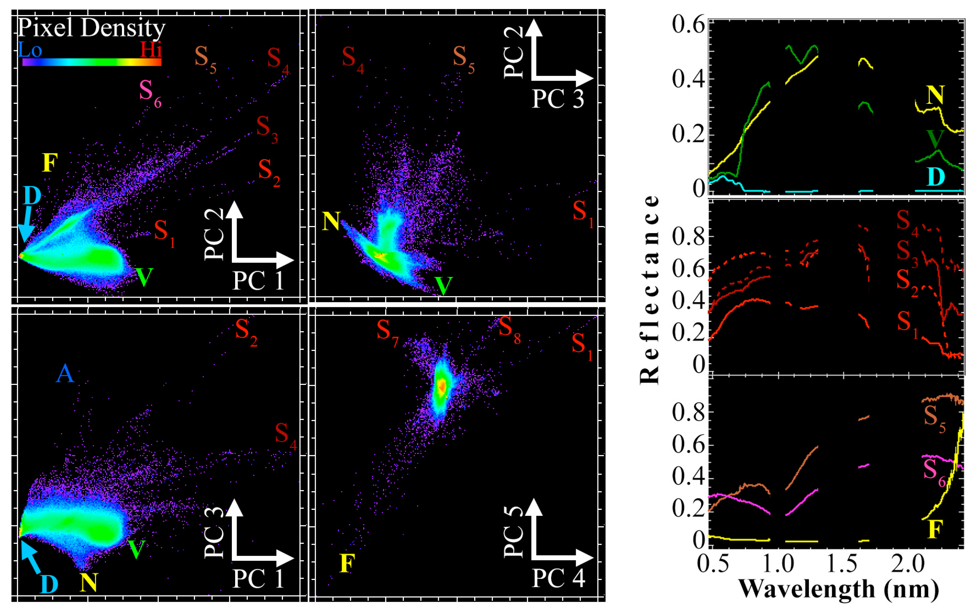
PCA-based characterization of high variance spectral features in the AVIRIS-3 mosaic is shown in Figure 3. All three pairwise projections of the first three dimensions of the spectral feature space are shown, as well as PC 4 vs. 5. The bulk of the pixels clearly occupy a dense mixing continuum bounded by Dark (D, thermokarst lakes, shallow coastal waters, and structural shadow), green Vegetation (V, grasses and forbs covering the permafrost), and nonphotosynthetic vegetation (N, senescent natural vegetation). These N, V, D endmember spectra are retained for use in the mixture residual (below).

Figure 3.
Principal Component based spectral feature space of the AVIRIS-3 dataset. The natural permafrost + thermokarst background forms a mixing space between Dark (D), green vegetation (V), and nonphotosynthetic vegetation (N) endmembers. This mixing continuum dominates image variance. Anthropogenic substrates (S1–S6) and processes, like Flaring (F), are spatially sparse but spectrally highly distinct, forming excursions from the mixing space. Some human materials are characterized by consistent absorption features, like the SWIR absorption at 2.2 microns and longer wavelengths characteristic of many polymers. Anthropogenic materials are prominent in the PC transform, but full characterization is made challenging by depth of the embedding space (many PCs to explore) and redundancy (same spectra identified by multiple pairs of PC dimensions). Here we show examples through PC5, but no obvious stopping point is evident.
Reflectance spectra of anthropogenic materials (hydrocarbon extraction and transmission infrastructure) and emission spectra of methane Flaring (F) diverge from the mixing continuum but are dispersed broadly across multiple mutually interacting PC dimensions. While we show projections through PC 5 here, no clear justification exists for a natural stopping point. As is common with imaging spectroscopy datasets [16,17,18], the preponderance of overall image variance (>99.6%) is partitioned into the first three dimensions. Clearly, PCA of reflectance alone is an inefficient method for characterizing the full spectral diversity of this complex dataset.
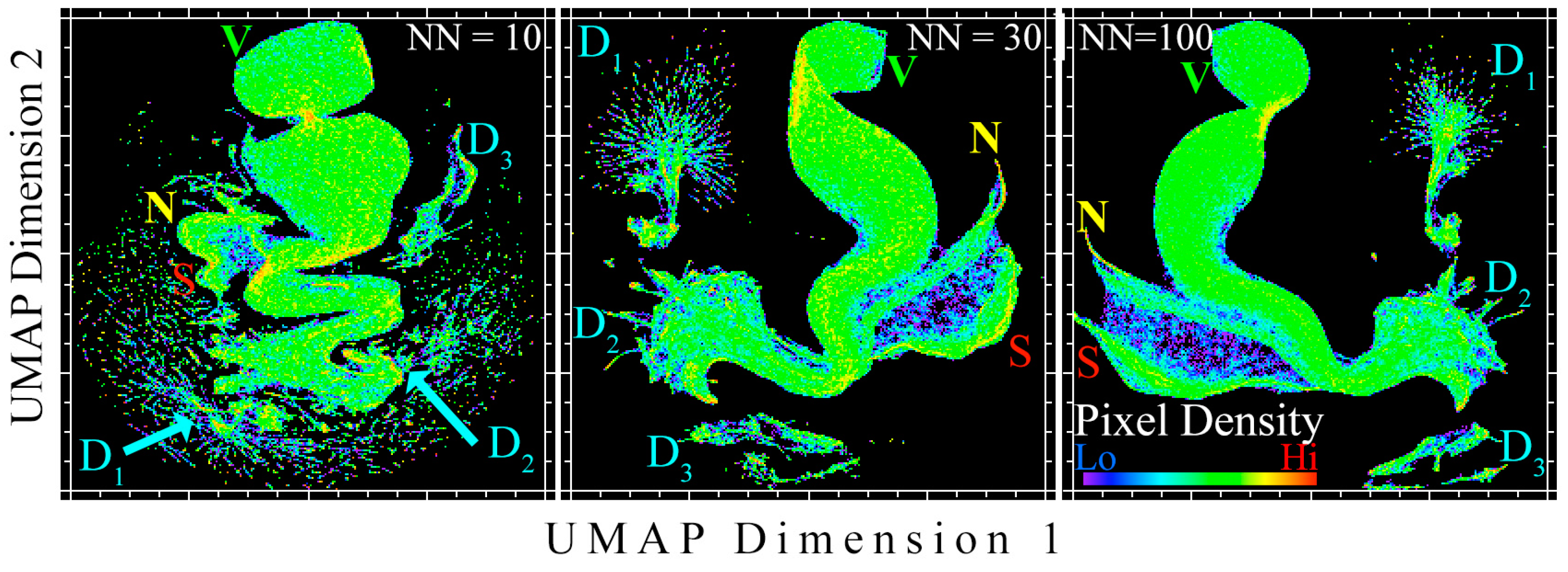
UMAP-based characterization of AVIRIS-3 reflectance is shown in Figure 4. The effect of the Nearest Neighbor (NN) hyperparameter is illustrated in the three panels. Low values, for example NN = 10 (left) are capable of capturing the primary mixing manifold but also generate a very large number of small clusters. Many of these small clusters correspond to image artifacts (e.g., tracing individual lines along-track), suggesting that this hyperparameter setting is effectively fitting noise. High values, for example NN = 100 (right) effectively resolve most of this behavior but can lose important low-variance details. For this dataset, we found an intermediate choice (center, NN = 30) achieved an effective balance of retaining subtle low-variance features while minimizing image artifacts.
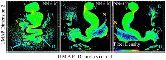
Figure 4.
2D UMAP spectral feature space of AVIRIS-3 reflectance. Additional Dark endmembers (D1–D3) are readily identified using UMAP but not using PCs 1 through 5 since their contribution to overall image variance is small. Mixing continua (e.g., from D2 to V and N) endmembers are also clearly visible. The full complexity of the anthropogenic substrates (S) collapses onto a single submanifold which can be easily identified and isolated for targeted analysis. The primary UMAP hyperparameter, the number of Nearest Neighbors (NN), has a clear impact on manifold structure. Low values of NN (left) result in identification of a very large number of internally consistent but globally incoherent clusters which are effectively fitting to sensor/atmospheric correction noise. High values of NN (right) capture global manifold topology but can lose important low-variance details. An intermediate value (center) was selected for subsequent work. Spectra for D1 and D3 are shown on Figure 5.
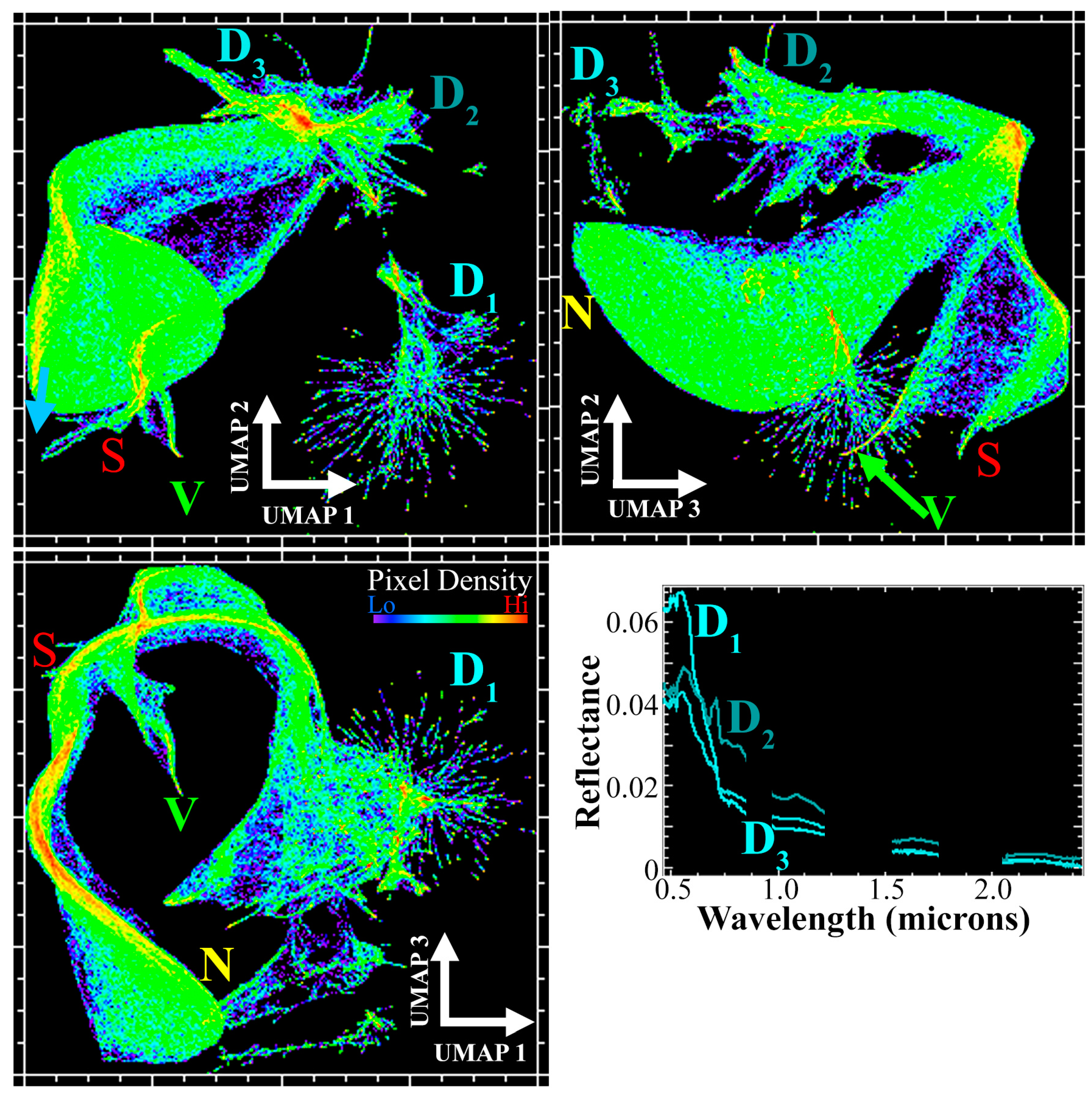
UMAP also offers a choice of embedding space dimension. Figure 4 uses the simplest useful embedding dimension (2D) in order to illustrate the effect of NN sensitivity. Analyses using smaller NN values (e.g., 10) more effectively capture local variance, but can also decompose into a stippled periphery of disconnected points. Higher NN values (e.g., 100) emphasize global variance, thus reducing the stippling effect but also losing potentially important but subtle local details. In contrast, Figure 5 illustrates the effect of increasing the embedding dimension to 3D for a single choice of NN (here, NN = 30). The manifold now fills out a larger volume, enabling greater separation between clusters. While a 3D embedding space is more complex for the analyst to explore, the greater detail afforded can offer key insights into endmember variability.
Interestingly, the clearest structure present in UMAP of the reflectance mosaic is the variable reflectance signatures present in the Dark fraction (D1, D2, and D3). These are readily identifiable in both the 2D and 3D projections. In map space, these correspond clearly to significant differences within and among bodies of water. Example spectra from each submanifold are shown in the lower right of Figure 5. Subtle but consistent spectral differences are observed throughout the spectrum (but particularly at visible wavelengths), consistent with compositional variability associated with turbidity and chlorophyll.
In both 2D and 3D UMAPs, the bulk of the pixels clearly emerge as multiple mixing continua emanating from D2. These primarily reflect binary mixtures towards N, V, and anthropogenic surfaces. While anthropogenic materials are clearly more easily discriminated (better clustered) in UMAP than in PCA, important uncertainties remain in the determination of the boundary of the anthropogenic cluster, particularly as it mixes with V and N.

Figure 5.
3D UMAP feature space of AVIRIS-3 reflectance. Complexity is even more evident in the shallow water (Dark 1–3, or D1–D3) endmembers in the 3D embedding than the 2D embedding. Nonphotosynthetic vegetation (N), green vegetation (V) and anthropogenic substrate (S) EMs are present, but less clearly identifiable. Inspection of the embedding image (Figure 6) shows that the UMAP clusters are capturing spatially coherent features.
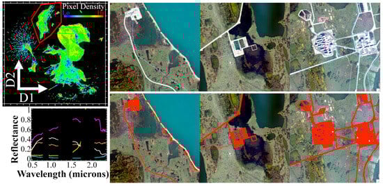
Figure 6.
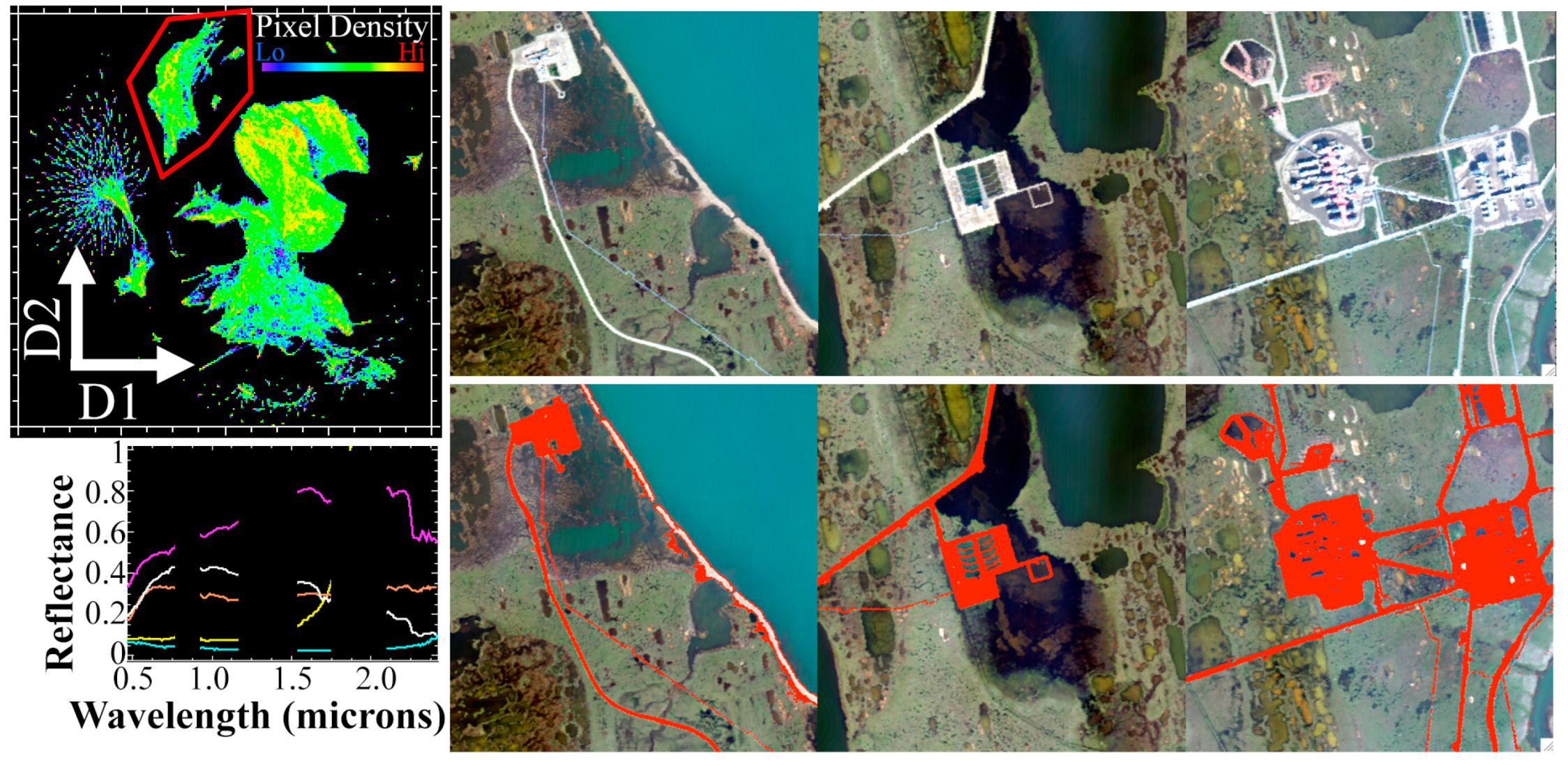
2D UMAP feature space of AVIRIS-3 spectral mixture residual. After removing the underlying mixing continuum, anthropogenic surfaces and processes are cleanly separable from the rest of the image (red polygon on feature space, red region of interest on image mosaic). Base image is a true color composite. A broad diversity of spectra (lower left) are contained within the statistically separable submanifold, corresponding to a wide range of infrastructure, including roads, pipelines, and extraction facilities. Some natural littoral features are also captured.
Figure 5.
3D UMAP feature space of AVIRIS-3 reflectance. Complexity is even more evident in the shallow water (Dark 1–3, or D1–D3) endmembers in the 3D embedding than the 2D embedding. Nonphotosynthetic vegetation (N), green vegetation (V) and anthropogenic substrate (S) EMs are present, but less clearly identifiable. Inspection of the embedding image (Figure 6) shows that the UMAP clusters are capturing spatially coherent features.
Next, we compute the spectral mixture residual using the N, V, and D local endmember spectra derived from the above PC analysis of the reflectance. As shown in the 2D UMAP embedding in the upper left of Figure 5, the mixture residual effectively removes the bulk of the contribution of the mixing continuum to the UMAP embedding. Here, statistical connectivity relations are broken between pixels associated with anthropogenic materials and pixels associated with natural tundra landscape, resulting in effectively complete statistical separation of the anthropogenic and natural landscapes. At the same time, connectivity relations among pixels within the anthropogenic cluster are preserved, structuring the manifold into interpretable endmember tendrils (example spectra shown in lower left). This allows for straightforward mapping of the built environment, and isolation of these pixels for targeted subsequent characterization.
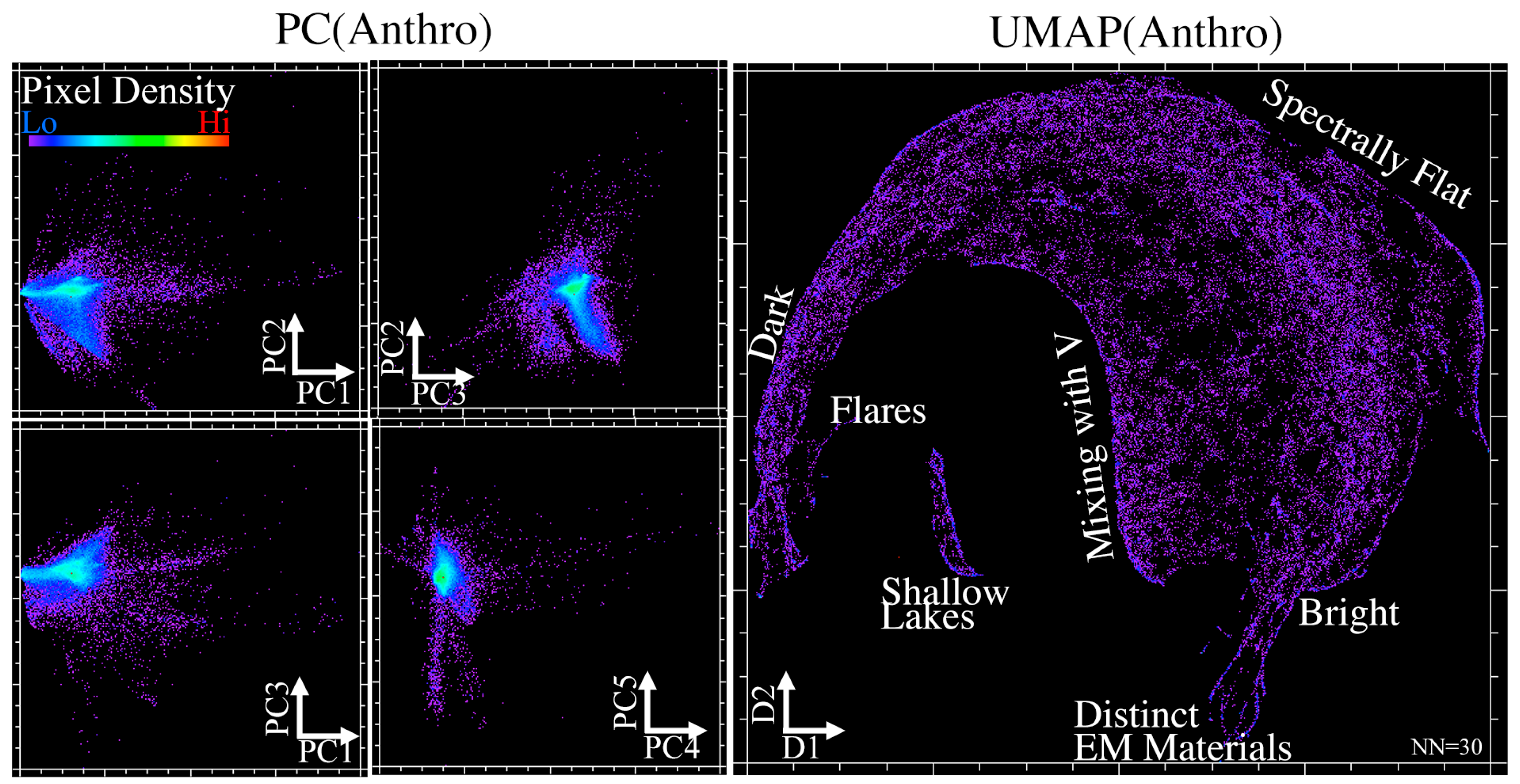
Targeted characterization of the pixels within the anthropogenic cluster is shown in Figure 7. Here, useful information is retrieved from both the PC and UMAP approaches. In both, a primary albedo-based mixing continuum exists, from a Dark endmember to a set of brighter, distinct EM materials. Methane flares are also evident in both spaces. UMAP locates a cluster of shallow lakes, which is not evident from the low-order PC space. Interestingly, a set of pixels mixing with the V endmember spectrum is also identified by UMAP. This corresponds to pixels which capture spatial mixtures of tundra vegetation with long, rectilinear pipeline infrastructure. The ability of the approach to identify these mixed pixels demonstrates that it is capable of resolving important, challenging edge cases.
Figure 7.
Spectral diversity within the anthropogenic pixels identified from the UMAP(MR) space as shown by both PCs (left) and targeted UMAP (right). Spaces are sparser because most of the image is now excluded. UMAP clearly shows the albedo continuum, culminating in multiple tendrils near the bottom of the space, each of which corresponds to a distinct reflectance spectrum. Mixed pixels are clearly identifiable from each edge of the manifold. In contrast, the PC space manifests as a spiky hyperball, with individual mixing lines emanating from the body of the point cloud. In some cases, by not requiring statistical connectivity, the PCs are better able to identify compositional gradients among small numbers of pixels.
3.2. Research Question 2: Effect of Spatial Resolution
The effect of 30 m resolution (roughly representative of most current and planned spaceborne imaging spectrometers) is shown in Figure 8. Here, the mosaic was spatially convolved with a low-pass Gaussian blurring kernel with a Full Width at Half Maximum of 8 pixels (32.8 m) to simulate a hypothetical spaceborne imaging spectrometer. The top panel shows PC-based (left) and UMAP-based (right) characterization of this spatially coarsened reflectance product. Here, the D to V spectral continuum that dominates the image area is still present in both PC and UMAP, but the N and S spectra are less separable. Less complexity is also evident in the water bodies. Application of the mixture residual (bottom panel) is ineffective at resolving additional endmembers in either PC (MR) or UMAP (MR) space. On this particular landscape, it is evident that a 30 m ground sampling distance so severely undersamples the characteristic scale of infrastructure that even imaging spectrometers are likely to struggle with identification of the full complexity of anthropogenic spectra. A more comprehensive illustration of the effects of spatial resolution on all dimensionality reduction approaches used in this study is shown in Appendix A.
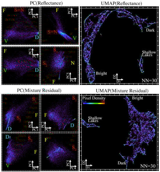
Figure 8.
Effect of spatial resolution on the characterization approach. Here we convolve the 4.1 m AVIRIS-3 reflectance mosaic with a low pass Gaussian blurring kernel to simulate the point spread function of a hypothetical 30 m resolution spaceborne imaging spectrometer. The resulting feature spaces are obviously much sparser. Broad spectral gradients corresponding to land cover types are evident, but clearly insufficient pixel density is present for either dimensionality reduction approach to resolve many important individual materials. Letter labels refer to the same endmember materials as Figure 3, Figure 4 and Figure 5.
3.3. Research Question 3: Effect of Spectral Resolution
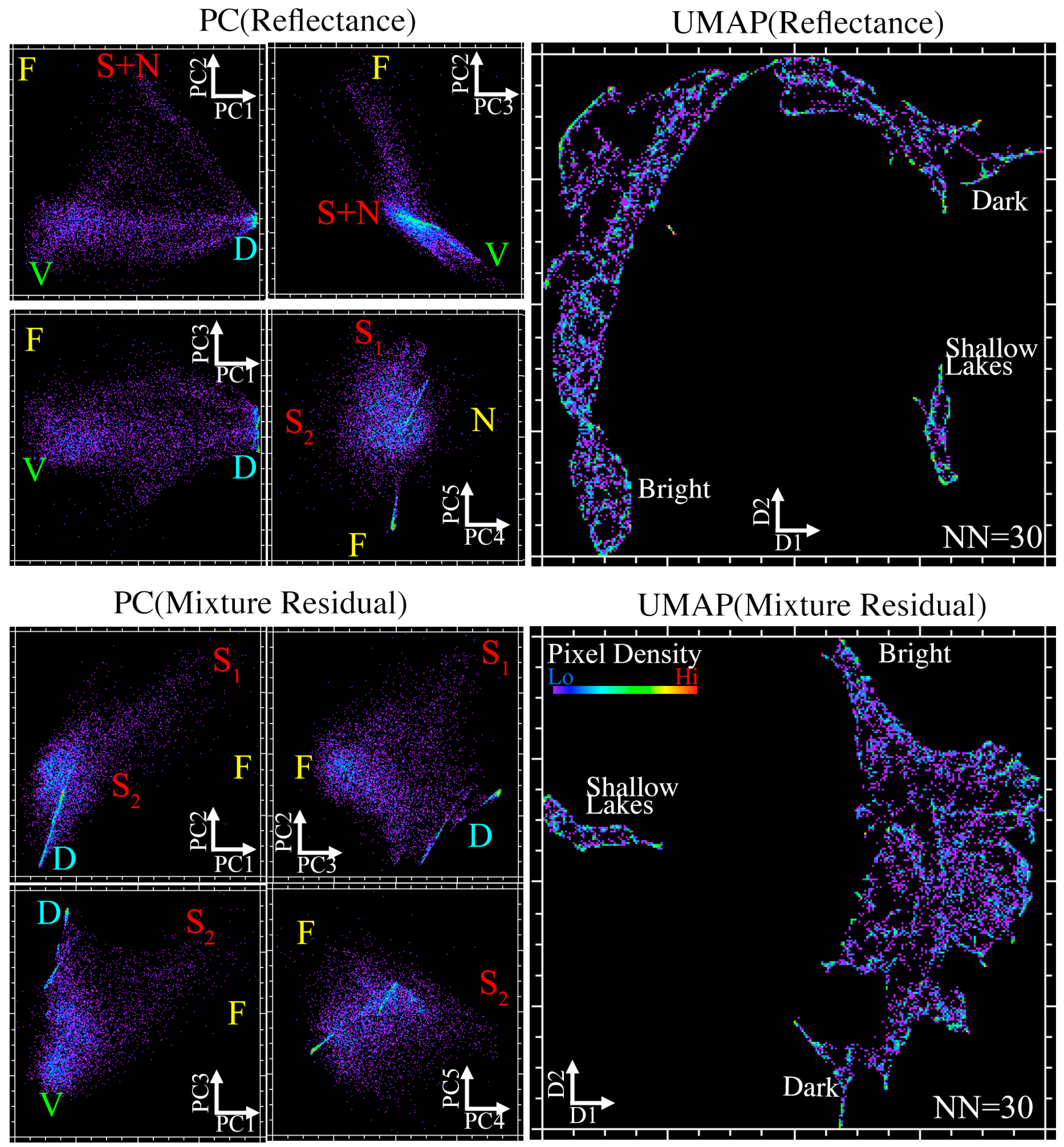
The effect of loss of spectral resolution is shown in Figure 9. Here, AVIRIS-3 pixel spectra were spectrally convolved with the spectral response function of the Sentinel-2A multispectral imager. As before, the top panel shows PC-based (left) and UMAP-based (right) characterization of this spectrally coarsened reflectance product. Both PC and UMAP are much more similar to the AVIRIS-3 results than for the spatially coarsened simulation. Shallow water variability still dominates the UMAP space. Anthropogenic materials are clearly more separable from nonphotosynthetic vegetation than in the spatially coarsened simulation. The PC (MR) transformation is effective in resolving several important classes of spectra (e.g., painted pipelines vs. polymer roofs vs. roads), but examination of the multispectral signatures alone severely limits confident diagnosis of material composition. Anthropogenic materials do emanate as a distinct submanifold in the UMAP (MR) space, but the reduced spectral resolution results in a lack of complete separability from the main mixing continuum. On this particular landscape, it is evident that this approach does still yield useful results for multispectral imagers but is unable to discriminate the full range of spectra that are identified from the AVIRIS-3 dataset.
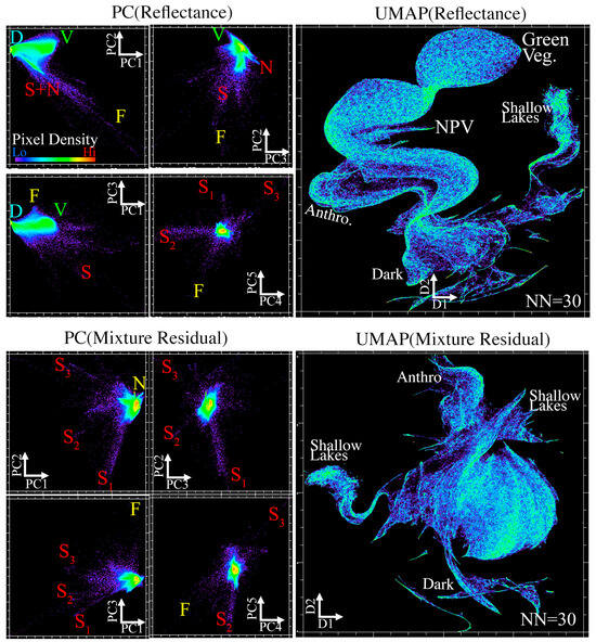
Figure 9.
Effect of spectral resolution on the characterization approach. Here we convolve the AVIRIS-3 reflectance mosaic with the spectral response function of the Sentinel-2A multispectral imager to simulate the effect of spectral resolution, while holding spatial resolution constant. Shallow water still dominates the UMAP manifold structure. Anthropogenic materials still form an appreciable submanifold, but it is not fully separable from the main manifold even after pretreatment with the spectral mixture residual. Interested readers may benefit from comparison to Figure 6 of [17]. Letter labels refer to the same endmember materials as Figure 3, Figure 4 and Figure 5.
4. Discussion
4.1. Synthesis of Key Results
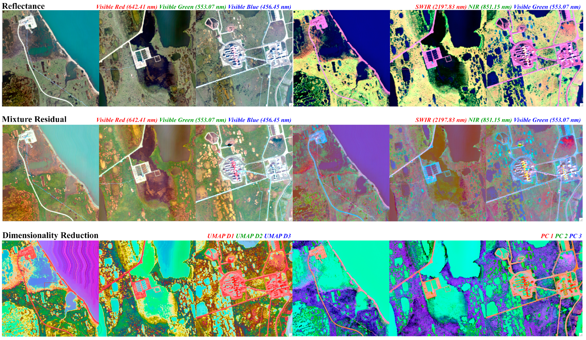
Figure 10 summarizes the visual appearance of the map-projected data in this analysis. The top row shows the original AVIRIS-3 reflectance as true color (left) and false color (right) composites. Clearly, the bulk of the mosaic is dominated by natural tundra and shallow water, with spatially sparse infrastructure elements. The center row shows both true color (left) and false color (right) wavelengths of the spectral mixture residual. Here, substantial additional complexity is evident within the tundra and lakes, as well as within the buildings, pipelines, and roads of the built environment. The bottom row shows a comparison of the dimensionality reduction outputs of PCs (right) and UMAP dimensions (left). Here, the spectral diversity of the anthropogenic materials can be isolated and characterized in a targeted way. Notably, considerable additional spectral diversity exists in the tundra landscapes around the infrastructure. Fully characterizing the diversity in these natural landscapes has the potential to be an important and interesting future application of this approach. Interestingly, lakeshore sediments present an interesting crossover between the two cases, appearing at intermediate feature space locations between the anthropogenic materials and the remainder of the tundra background. Characterizing spectral variability in these targets also represents an interesting and potentially important avenue for future work.
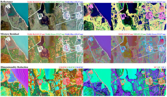
Figure 10.
Map view of key results. Top row shows true color (left) and false color (right) reflectance. Middle row shows true color (left) and false color (right) spectral mixture residual images. Bottom row shows dimensionality reduction results from UMAP dimensions (left) and PCs (right).
The results from Figure 6 and Figure 7 clearly demonstrate that this approach can be used to successfully partition and characterize spectral diversity in the built environment in arctic tundra landscapes. While the subset of these results associated with discrete mapping of pixels with high amplitude differences in spectral continuum could clearly be replicated using multispectral imagery, continuous field characterization and spectral identification of compositional diversity of course requires spectroscopic imagery. Further, the results from Figure 8 and Figure 9 demonstrate that reduction in either spatial or spectral resolution have significant impacts on the spectral diversity that can be retrieved in this environment. We suspect the dependence on spatial resolution to be at least partially explained by the process of computing weighted averages of larger and larger sets of neighboring pixels substantially reducing the occurrence of the relatively rare, spatially dispersed targets of interest to the study. This could then result in a degradation of topological complexity of the UMAP manifold, and a concomitant reduction in spectral separability between the targets of interest and the natural tundra background. This is consistent with numerous previous studies focusing on other aspects of this landscape which have found significant scale dependence and a requirement for high spatial resolution observations (e.g., [40]).
The approach illustrated in this analysis could potentially be used for a broad range of practical applications. Applications requiring characterization of spatially sparse targets with important but subtle spectral diversity would be of most relevance. In addition to the built environment, application areas could include geologic units, agricultural basins, water bodies, and more. Given the results of this study, such applications should thus consider the relationship between the spatial scale of the objects being observed and the ground sampling distance of the imaging sensor, with consideration for further refinements of the model as required on a case-by-case basis.
The heterogeneous nature of the Arctic environment requires high-resolution remote sensing products coupled with in situ and airborne retrievals [41]. The discontinuous permafrost tundra environments represent numerous biomes aboveground, with even more belowground diversity. The diversity of each region also means that the thaw processes are incongruent, leading to regions of significant permafrost thaw, water pooling and infrastructure impacts, and other regions that are more stable. While the airborne retrievals from the Arctic-Boreal Vulnerability Experiment (ABoVE) and AVIRIS-3 missions provide mid-scale observations, in between satellite remote sensing and small-scale in situ work, higher resolution is still required as the tundra changes rapidly. Ongoing field campaigns across the spring, summer, and fall seasons will be necessary for the successful monitoring of environmental changes as the Arctic warms.
4.2. Implications for Other Arctic Studies
Climate change in the Arctic is being documented at rapid rates, sometimes quantified as up to four times the global average [42]. Implications for social-ecological systems are myriad, including concern for the ability of Arctic communities to meet basic needs pertaining to water availability [43], subsistence hunting [44], as well as marine and aviation transport of goods and medical care [45].
Permafrost thaw is associated with methane releases [46] and threats to infrastructure stability [47]. Alaska’s petroleum resources coincide with permafrost along the North Slope region, where many of these vulnerabilities overlap [48]. The operation of hydrocarbon production infrastructure generates heat and locally accelerates permafrost thaw [49,50]. Extractive activities also increase vulnerability to oil spills [51] and can disrupt the habitats of organisms used for subsistence hunting [52]. Areas with hydrocarbon production infrastructure can thus reasonably be considered hotspots for disruption of social-ecological systems.
4.3. Limitations
While the results of this study are promising, no approach is without limitations. For the specific targets of interest in this study, spatial resolution is a key concern. Even with the spectral performance of AVIRIS-3, sufficient coarsening of spatial resolution can result in sufficient sparsity to overwhelm UMAP (or any manifold learning algorithm). Further, for some landscapes (e.g., evaporites, bedrock outcrops, lakes, or coastal waters), it is likely that the generalized mixture model used here could be ill-constructed for a local landscape and thus yield unsatisfactory results. Computational factors may additionally limit the operational implementation of this approach at extensive spatial scales. While the UMAP algorithm is considerably less computationally intensive than other manifold learning approaches, the computational resources required (notably RAM) scale with the size of the study area.
4.4. Avenues for Future Work
Moving forward, several potentially useful avenues exist to extend the scope and utility of this approach. Generalized application as an anomaly characterization tool would be strengthened by application in other types of landscapes, for instance in agricultural systems with cover crops [53] and pasture degradation [54], spatial scaling in natural plant communities [55], or spatial variability within methane plumes [56]. Utility could also extend to the spatiotemporal domain, for instance in the characterization of vegetation phenology [57]. Valuable insight could also be derived from comparison against, and eventual synergistic cooperation with, other approaches to anomaly detection and characterization, for instance, Convolutional Neural Network (CNN) approaches to cloud screening [58]. Global generality should also be further addressed using globally standardized endmembers (e.g., [59]), as well as fully constrained and multiple endmember models [60], with specific evaluation of the relationship to, and potential synergy with, joint characterization [17,27,38].
5. Conclusions
We illustrate an approach to characterize spectral diversity of sparse targets in a smoothly varying background. This approach proceeds in two main steps: first, through characterization and removal of background using generalized spectral mixture model; and second, by using nonlinear dimensionality reduction via manifold learning on the spectral mixture residual. The approach is shown to be capable of effective statistical discrimination between our sparse target (anthropogenic materials) from our spatially extensive background (Arctic permafrost). Identification of sparse endmember spectra is dependent on both spatial and spectral resolution. The most comprehensive set of spectra, and most effective discrimination between target and background, is achieved at the native ground sampling distance and spectral resolution of the AVIRIS-3 reflectance. Spatially coarsening the imagery to 30 m (analogous to current and planned spaceborne imaging spectrometers) results in substantial loss of target spectra. Spectrally coarsening the imagery to match the Sentinel-2A MultiSpectral Imager retains important details in the characterization, but results in a loss of target discrimination efficacy (as well as loss of diagnostic absorption features). Overall, these results suggest this approach may be a promising avenue for future work seeking to characterize spectral diversity of sparse targets embedded in an extensive but linearly describable spectral background.
Author Contributions
Conceptualization, D.S.; methodology, D.S.; software, D.S.; formal analysis, D.S.; investigation, all authors; resources, D.S., K.M. and L.B.; writing—original draft preparation, D.S. and E.J.B.; writing—review and editing, all authors; visualization, D.S.; supervision, D.S. and L.B.; project administration, L.B.; funding acquisition, L.B., K.M. and D.S. All authors have read and agreed to the published version of the manuscript.
Funding
The authors gratefully acknowledge funding from the NASA Land-Cover/Land Use Change program (Grant #NNH21ZDA001N-LCLUC). D.S. acknowledges further funding from the EMIT Science and Applications Team program (Grant #80NSSC24K0861), the NASA Remote Sensing of Water Quality program (Grant #80NSSC22K0907), the NASA Applications-Oriented Augmentations for Research and Analysis Program (Grant #80NSSC23K1460), the NASA Commercial Smallsat Data Analysis Program (Grant #80NSSC24K0052), the NASA FireSense Program (Grants #80NSSC24K1320 and 80NSSC24K0145), the USDA NIFA Sustainable Agroecosystems program (Grant #2022-67019-36397), the USDA AFRI Rapid Response to Extreme Weather Events Across Food and Agricultural Systems program (Grant #2023-68016-40683), the California Climate Action Seed Award Program, and the NSF Signals in the Soil program (Award #2226649).
Data Availability Statement
All data used for this study are available at the web portals given in the text.
Acknowledgments
D.S. thanks C. Small for helpful feedback on the study design, as well as over a decade of useful and informative conversations. The authors also thank four anonymous reviewers, whose comments improved the quality of the manuscript.
Conflicts of Interest
The authors declare no conflicts of interest.
Appendix A
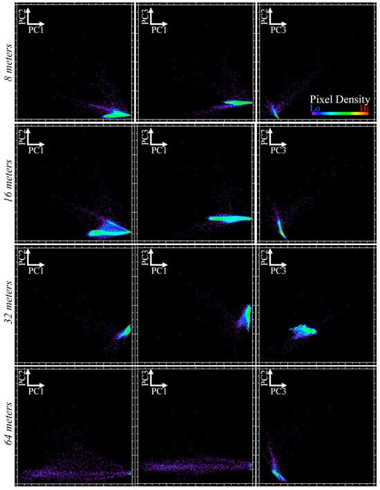
Figure A1.
Sensitivity of 3D covariance-based Principal Component spectral feature space of AVIRIS-3 reflectance to coarsening spatial resolution. The body of the point cloud is compressed towards the corner of the scatterplots to accommodate the wide range of spatially sparse high-variance pixels associated with emission spectra from methane flaring and spurious BRDF effects. A clear step change occurs between 16 and 32 m resolution, surprisingly consistent with [61].
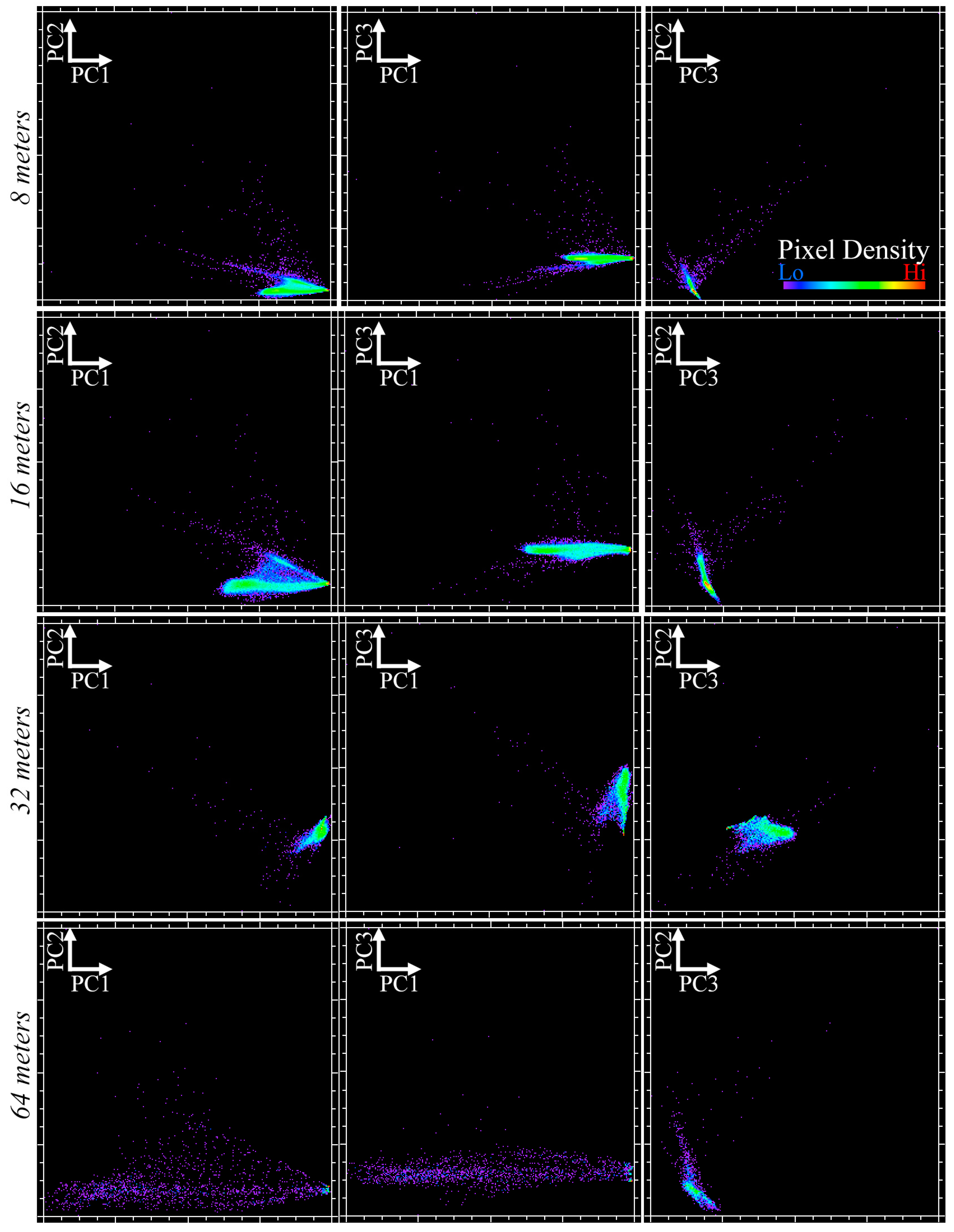
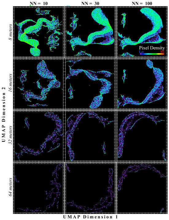
Figure A2.
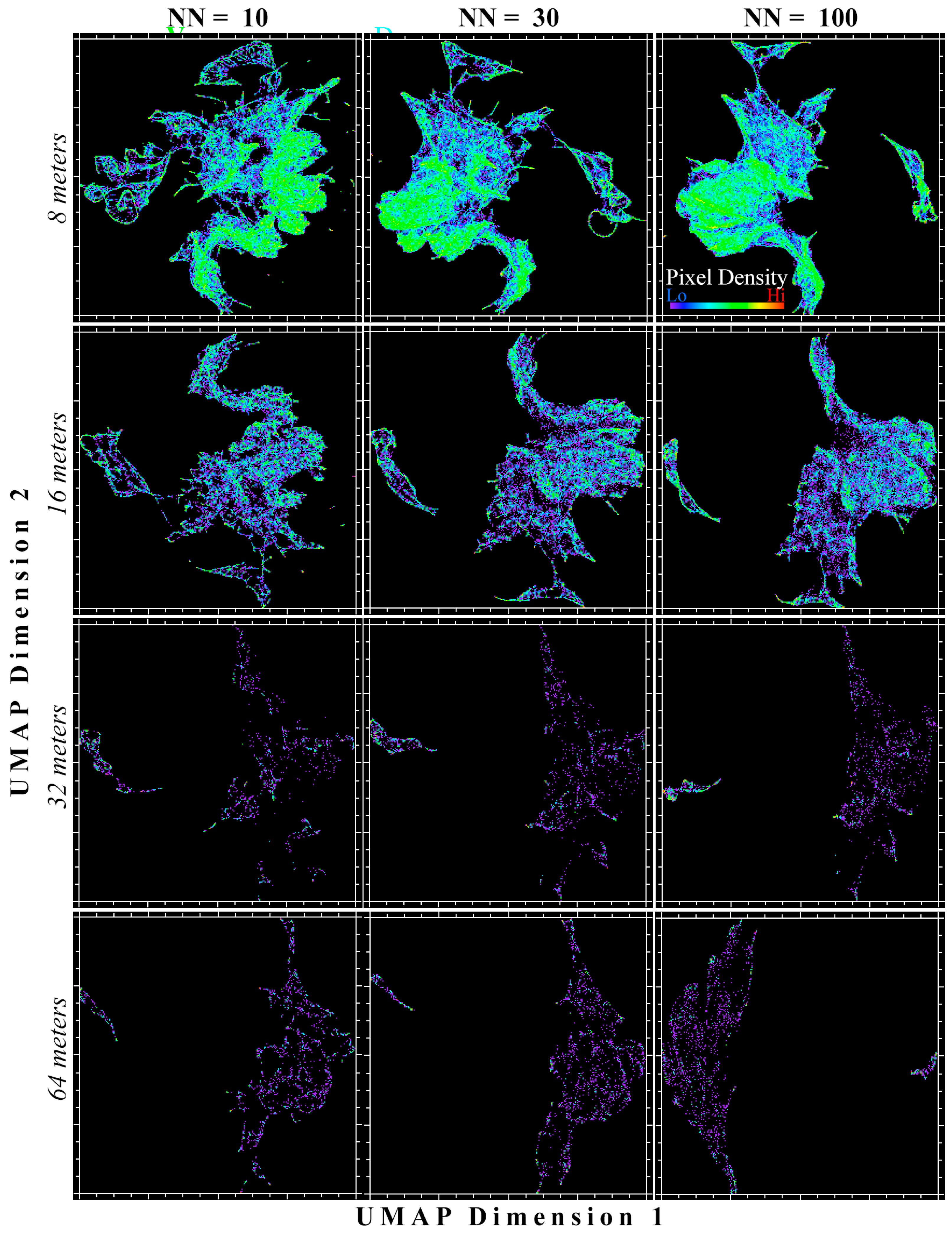
Sensitivity of 2D UMAP spectral feature space of AVIRIS-3 reflectance to coarsening spatial resolution. Manifold connectivity is greatest with fine spatial resolution (above) and degrades as resolution coarsens (below). For this dataset, 8 m resolution data (top row) captures similar manifold topology to the full 4 m resolution reflectance data (compare to Figure 4), while 64 m resolution data (bottom row) retains only the most generic manifold properties.
Figure A2.
Sensitivity of 2D UMAP spectral feature space of AVIRIS-3 reflectance to coarsening spatial resolution. Manifold connectivity is greatest with fine spatial resolution (above) and degrades as resolution coarsens (below). For this dataset, 8 m resolution data (top row) captures similar manifold topology to the full 4 m resolution reflectance data (compare to Figure 4), while 64 m resolution data (bottom row) retains only the most generic manifold properties.
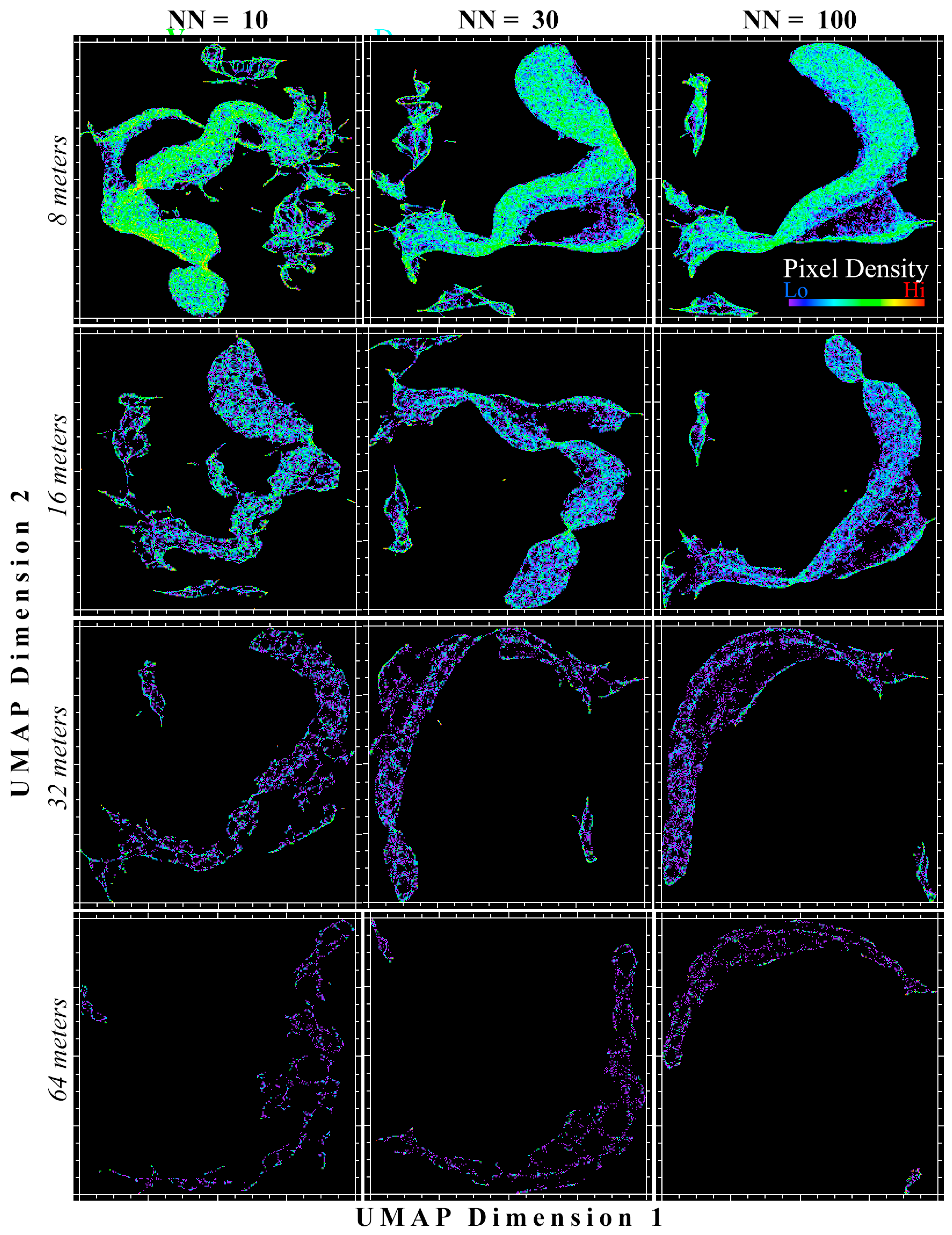
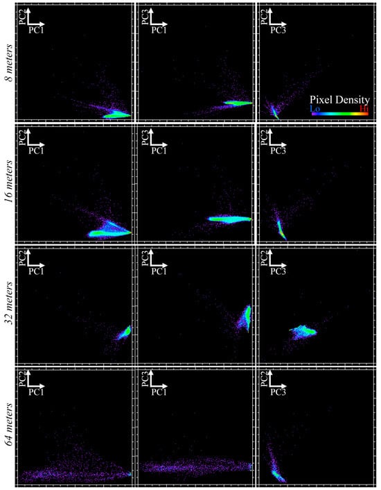
Figure A3.
Sensitivity of 3D covariance-based Principal Component spectral feature space of AVIRIS-3 mixture residual reflectance to coarsening spatial resolution. The body of the point cloud is compressed towards the corner of the scatterplots to accommodate the wide range of spatially sparse high-variance pixels associated with emission spectra from methane flaring and spurious BRDF effects. As with Figure A3, a clear step change occurs between 16 and 32 m resolution.
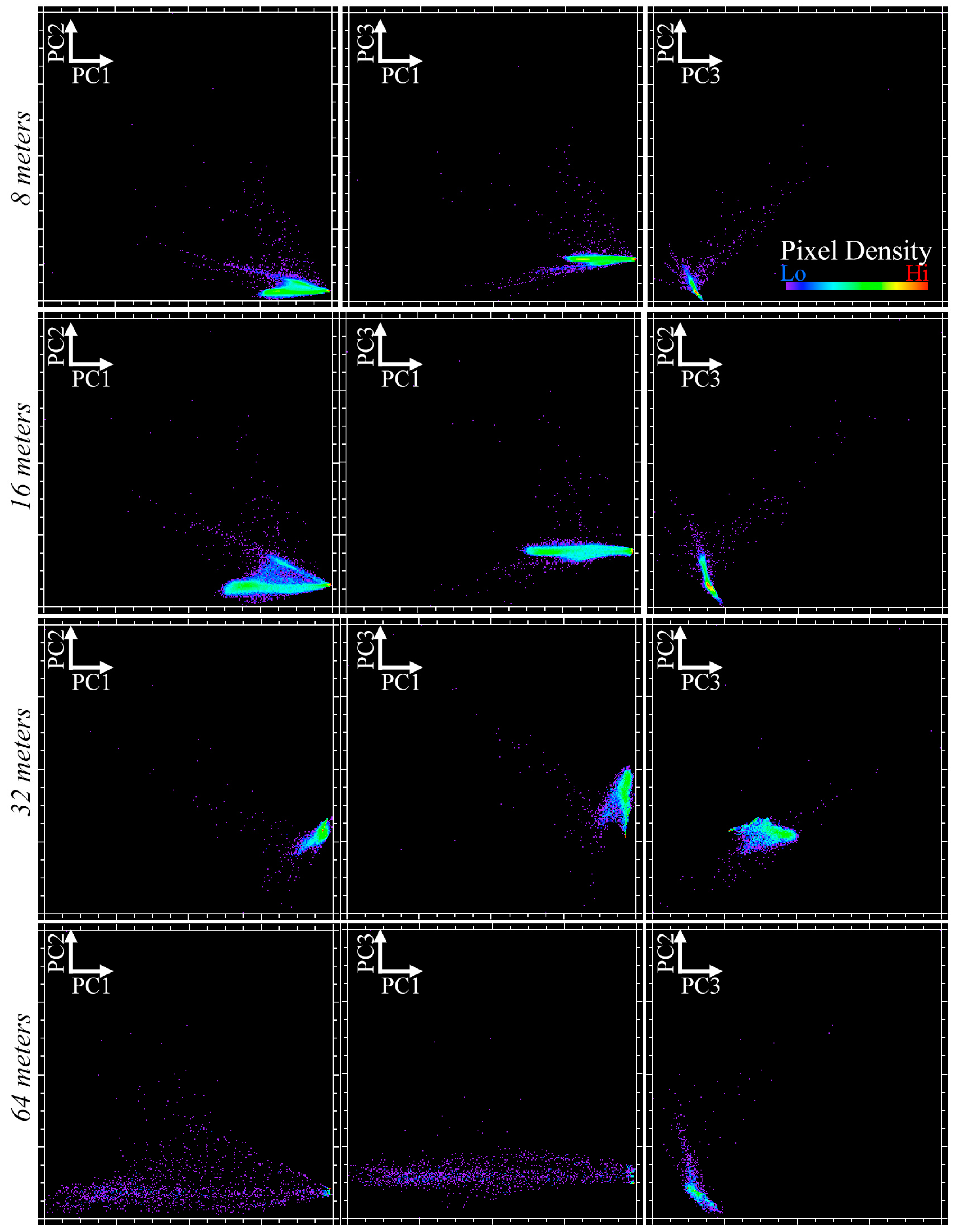
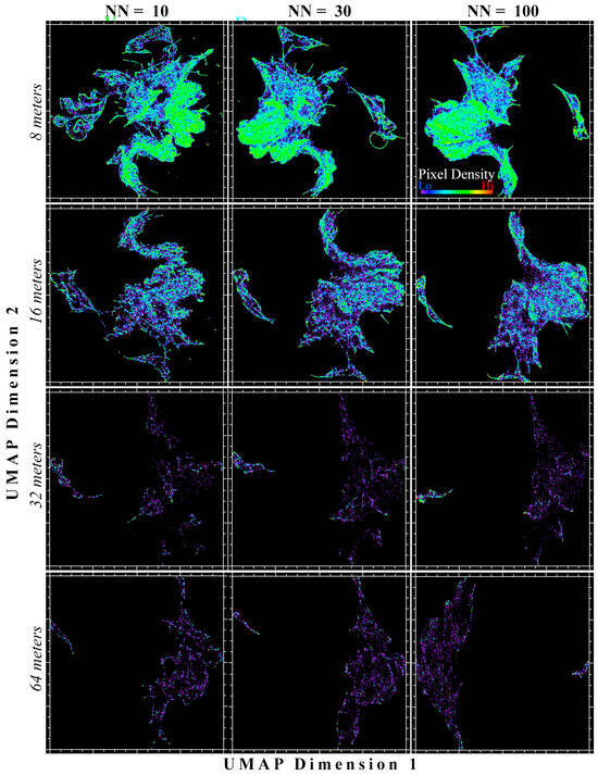
Figure A4.
Sensitivity of 2D UMAP spectral feature space of AVIRIS-3 mixture residual reflectance to coarsening spatial resolution. As with UMAP (Reflectance), manifold connectivity is greatest with fine spatial resolution (above) and degrades as resolution coarsens (below).
Figure A4.
Sensitivity of 2D UMAP spectral feature space of AVIRIS-3 mixture residual reflectance to coarsening spatial resolution. As with UMAP (Reflectance), manifold connectivity is greatest with fine spatial resolution (above) and degrades as resolution coarsens (below).
References
- Turin, G. An Introduction to Matched Filters. IRE Trans. Inf. Theory 1960, 6, 311–329. [Google Scholar] [CrossRef]
- Woodward, P.M. Information Theory and the Design of Radar Receivers. Proc. IRE 1951, 39, 1521–1524. [Google Scholar] [CrossRef]
- Boardman, J.W. Leveraging the High Dimensionality of AVIRIS Data for Improved Sub-Pixel Target Unmixing and Rejection of False Positives: Mixture Tuned Matched Filtering; NASA Jet Propulsion Laboratory: Pasadena, CA, USA, 1998; Volume 97, pp. 55–56.
- Harsanyi, J.C.; Chang, C.-I. Hyperspectral Image Classification and Dimensionality Reduction: An Orthogonal Subspace Projection Approach. IEEE Trans. Geosci. Remote Sens. 1994, 32, 779–785. [Google Scholar] [CrossRef]
- Reed, I.S.; Yu, X. Adaptive Multiple-Band CFAR Detection of an Optical Pattern with Unknown Spectral Distribution. IEEE Trans. Acoust. Speech Signal Process. 1990, 38, 1760–1770. [Google Scholar] [CrossRef]
- Thompson, D.; Leifer, I.; Bovensmann, H.; Eastwood, M.; Fladeland, M.; Frankenberg, C.; Gerilowski, K.; Green, R.; Kratwurst, S.; Krings, T. Real-Time Remote Detection and Measurement for Airborne Imaging Spectroscopy: A Case Study with Methane. Atmos. Meas. Tech. 2015, 8, 4383–4397. [Google Scholar] [CrossRef]
- Nasrabadi, N.M. Hyperspectral Target Detection: An Overview of Current and Future Challenges. IEEE Signal Process. Mag. 2013, 31, 34–44. [Google Scholar] [CrossRef]
- Pearson, K. LIII. On Lines and Planes of Closest Fit to Systems of Points in Space. Null 1901, 2, 559–572. [Google Scholar] [CrossRef]
- Ans, B.; Hérault, J.; Jutten, C. Architectures Neuromimétiques Adaptatives: Détection de Primitives. Proc. Cogn. 1985, 85, 593–597. [Google Scholar]
- Gordon, C. A Generalization of the Maximum Noise Fraction Transform. IEEE Trans. Geosci. Remote Sens. 2000, 38, 608–610. [Google Scholar] [CrossRef]
- Plaza, A.; Chang, C.-I. Fast Implementation of Pixel Purity Index Algorithm; SPIE: Bellingham, WA, USA, 2005; Volume 5806, pp. 307–317. [Google Scholar]
- Clark, R.N.; King, T.V. Automatic Continuum Analysis of Reflectance Spectra. In Proceedings of the 3rd Airborne Imaging Spectrometer Data Analysis Workshop; NASA NTRS N88-13770, Document ID 19880004388; Jet Propulsion Laboratory: Pasadena, CA, USA, 1987; pp. 138–142. [Google Scholar]
- Savitzky, A.; Golay, M.J. Smoothing and Differentiation of Data by Simplified Least Squares Procedures. Anal. Chem. 1964, 36, 1627–1639. [Google Scholar] [CrossRef]
- Crist, E.P.; Cicone, R.C. A Physically-Based Transformation of Thematic Mapper Data—The TM Tasseled Cap. IEEE Trans. Geosci. Remote Sens. 1984, GE-22, 256–263. [Google Scholar] [CrossRef]
- Kauth, R.J.; Thomas, G.S. The Tasselled Cap—A Graphic Description of the Spectral-Temporal Development of Agricultural Crops as Seen by LANDSAT. In Proceedings of the Symposium on Machine Processing of Remotely Sensed Data, West Lafayette, IN, USA, 29 July–1 August 1976; The Laboratory for Applications of Remote Sensing, Purdue University: West Lafayette, IN, USA, 1976; pp. 41–51. [Google Scholar]
- Sousa, D.; Brodrick, P.G.; Cawse-Nicholson, K.; Fisher, J.B.; Pavlick, R.; Small, C.; Thompson, D.R. The Spectral Mixture Residual: A Source of Low-Variance Information to Enhance the Explainability and Accuracy of Surface Biology and Geology Retrievals. J. Geophys. Res. Biogeosci. 2022, 127, e2021JG006672. [Google Scholar] [CrossRef]
- Sousa, D.; Small, C. Topological Generality and Spectral Dimensionality in the Earth Mineral Dust Source Investigation (EMIT) Using Joint Characterization and the Spectral Mixture Residual. Remote Sens. 2023, 15, 2295. [Google Scholar] [CrossRef]
- Sousa, D.; Small, C. Multisensor Analysis of Spectral Dimensionality and Soil Diversity in the Great Central Valley of California. Sensors 2018, 18, 583. [Google Scholar] [CrossRef]
- Small, C. The Landsat ETM+ Spectral Mixing Space. Remote Sens. Environ. 2004, 93, 1–17. [Google Scholar] [CrossRef]
- Small, C.; Milesi, C. Multi-Scale Standardized Spectral Mixture Models. Remote Sens. Environ. 2013, 136, 442–454. [Google Scholar] [CrossRef]
- Sousa, D.; Small, C. Globally Standardized MODIS Spectral Mixture Models. Remote Sens. Lett. 2019, 10, 1018–1027. [Google Scholar] [CrossRef]
- Sousa, D.; Small, C. Global Cross-Calibration of Landsat Spectral Mixture Models. Remote Sens. Environ. 2017, 192, 139–149. [Google Scholar] [CrossRef]
- Green, R.O.; Schaepman, M.E.; Mouroulis, P.; Geier, S.; Shaw, L.; Hueini, A.; Bernas, M.; McKinley, I.; Smith, C.; Wehbe, R. Airborne Visible/Infrared Imaging Spectrometer 3 (AVIRIS-3); IEEE: Big Sky, MT, USA, 2022; pp. 1–10. [Google Scholar]
- Bradley, C.L.; Thingvold, E.; Moore, L.B.; Haag, J.M.; Raouf, N.A.; Mouroulis, P.; Green, R.O. Optical Design of the Earth Surface Mineral Dust Source Investigation (EMIT) Imaging Spectrometer; Jet Propulsion Laboratory, National Aeronautics and Space Administration: Pasadena, CA, USA, 2020; Volume 11504, p. 1150402.
- Thompson, D.R.; Natraj, V.; Green, R.O.; Helmlinger, M.C.; Gao, B.-C.; Eastwood, M.L. Optimal Estimation for Imaging Spectrometer Atmospheric Correction. Remote Sens. Environ. 2018, 216, 355–373. [Google Scholar] [CrossRef]
- Thompson, D.R.; Brodrick, P.G.; Green, R.O.; Kalashnikova, O.; Lundeen, S.; Okin, G.; Olson-Duvall, W.; Painter, T. EMIT L2A Algorithm: Surface Reflectance and Scene Content Masks—Theoretical Basis; Earth Mineral Dust Source InvesTigation (EMIT); Jet Propulsion Laboratory, California Institute of Technology: Pasadena, CA, USA, 2020; p. 23.
- Sousa, D.; Small, C. Joint Characterization of Multiscale Information in High Dimensional Data. Adv. Artif. Intell. Mach. Learn. 2021, 1, 196–212. [Google Scholar] [CrossRef]
- McInnes, L. UMAP: Uniform Manifold Approximation and Projection for Dimension Reduction—Umap 0.5 Documentation. Available online: https://umap-learn.readthedocs.io/en/latest/ (accessed on 13 October 2022).
- Meilă, M.; Zhang, H. Manifold Learning: What, How, and Why. Annu. Rev. Stat. Appl. 2024, 11, 393–417. [Google Scholar] [CrossRef]
- van der Maaten, L.; Hinton, G. Visualizing Data Using T-SNE. J. Mach. Learn. Res. 2008, 9, 2579–2605. [Google Scholar]
- Donoho, D.L.; Grimes, C. Hessian Eigenmaps: Locally Linear Embedding Techniques for High-Dimensional Data. Proc. Natl. Acad. Sci. USA 2003, 100, 5591–5596. [Google Scholar] [CrossRef] [PubMed]
- Kim, D.H.; Finkel, L.H. Hyperspectral Image Processing Using Locally Linear Embedding; IEEE: Capri, Italy, 2003; pp. 316–319. [Google Scholar]
- Roweis, S.T.; Saul, L.K. Nonlinear Dimensionality Reduction by Locally Linear Embedding. Science 2000, 290, 2323–2326. [Google Scholar] [CrossRef] [PubMed]
- Jiale, Y.; Ying, Z. Visualization Method of Sound Effect Retrieval Based on UMAP. In Proceedings of the 2020 IEEE 4th Information Technology, Networking, Electronic and Automation Control Conference (ITNEC), Chongqing, China, 12–14 June 2020; Volume 1, pp. 2216–2220. [Google Scholar]
- Zhang, Q.; Liu, Y.; Fang, H. Manifold Learning-Based UMAP Method for Geochemical Anomaly Identification. Geochemistry 2024, 84, 126157. [Google Scholar] [CrossRef]
- Casanova, R.; Lyday, R.G.; Bahrami, M.; Burdette, J.H.; Simpson, S.L.; Laurienti, P.J. Embedding Functional Brain Networks in Low Dimensional Spaces Using Manifold Learning Techniques. Front. Neuroinform. 2021, 15, 740143. [Google Scholar] [CrossRef] [PubMed]
- Sousa, D.; Mayes, M.; Davis, F.; Fisher, J.B. Characterization of California Plant Communities with the Mixture Residual. In Proceedings of the Hyperspectral Imaging and Sounding of the Environment (HISE), Vancouver, BC, Canada, 19–23 July 2021; Optical Society of America: Vancouver, CA, USA, 2021; p. 2. [Google Scholar]
- Sousa, F.J.; Sousa, D.J. Hyperspectral Reconnaissance: Joint Characterization of the Spectral Mixture Residual Delineates Geologic Unit Boundaries in the White Mountains, CA. Remote Sens. 2022, 14, 4914. [Google Scholar] [CrossRef]
- Drusch, M.; Del Bello, U.; Carlier, S.; Colin, O.; Fernandez, V.; Gascon, F.; Hoersch, B.; Isola, C.; Laberinti, P.; Martimort, P. Sentinel-2: ESA’s Optical High-Resolution Mission for GMES Operational Services. Remote Sens. Environ. 2012, 120, 25–36. [Google Scholar] [CrossRef]
- Nelson, P.R.; Maguire, A.J.; Pierrat, Z.; Orcutt, E.L.; Yang, D.; Serbin, S.; Frost, G.V.; Macander, M.J.; Magney, T.S.; Thompson, D.R. Remote Sensing of Tundra Ecosystems Using High Spectral Resolution Reflectance: Opportunities and Challenges. J. Geophys. Res. Biogeosci. 2022, 127, e2021JG006697. [Google Scholar] [CrossRef]
- Miner, K.R.; Turetsky, M.R.; Malina, E.; Bartsch, A.; Tamminen, J.; McGuire, A.D.; Fix, A.; Sweeney, C.; Elder, C.D.; Miller, C.E. Permafrost Carbon Emissions in a Changing Arctic. Nat. Rev. Earth Environ. 2022, 3, 55–67. [Google Scholar] [CrossRef]
- Rantanen, M.; Karpechko, A.Y.; Lipponen, A.; Nordling, K.; Hyvärinen, O.; Ruosteenoja, K.; Vihma, T.; Laaksonen, A. The Arctic Has Warmed Nearly Four Times Faster than the Globe since 1979. Commun. Earth Environ. 2022, 3, 168. [Google Scholar] [CrossRef]
- Hayward, J.; Johnston, L.; Jackson, A.; Jamieson, R. Hydrological Analysis of Municipal Source Water Availability in the Canadian Arctic Territory of Nunavut. Arctic 2021, 74, 30–41. [Google Scholar] [CrossRef]
- Ayeb-Karlsson, S.; Hoad, A.; Trueba, M.L. ‘My Appetite and Mind Would Go’: Inuit Perceptions of (Im)Mobility and Wellbeing Loss under Climate Change across Inuit Nunangat in the Canadian Arctic. Humanit. Soc. Sci. Commun. 2024, 11, 277. [Google Scholar] [CrossRef]
- Debortoli, N.S.; Clark, D.G.; Ford, J.D.; Sayles, J.S.; Diaconescu, E.P. An Integrative Climate Change Vulnerability Index for Arctic Aviation and Marine Transportation. Nat. Commun. 2019, 10, 2596. [Google Scholar] [CrossRef] [PubMed]
- Abakumov, E.; Petrov, A.; Polyakov, V.; Nizamutdinov, T. Soil Organic Matter in Urban Areas of the Russian Arctic: A Review. Atmosphere 2023, 14, 997. [Google Scholar] [CrossRef]
- Scheer, J.; Tomaškovičová, S.; Ingeman-Nielsen, T. Thaw Settlement Susceptibility Mapping for Roads on Permafrost-Towards Climate-Resilient and Cost-Efficient Infrastructure in the Arctic. Cold Reg. Sci. Technol. 2024, 220, 104136. [Google Scholar] [CrossRef]
- Bushnell, E.; Miner, K.; Sousa, D.; Baskaran, L. A Review of Emergent Vulnerabilities Indices in the Alaskan Arctic. ESS Open Arch. 2024. [Google Scholar] [CrossRef]
- Wang, J.; Zhang, F.; Yang, Z.J.; Yang, P. Experimental Investigation on the Mechanical Properties of Thawed Deep Permafrost from the Kuparuk River Delta of the North Slope of Alaska. Cold Reg. Sci. Technol. 2022, 195, 103482. [Google Scholar] [CrossRef]
- Cao, Y.; Ma, W.; Li, G.; Gao, K.; Li, C.; Chen, D.; Shang, Y.; Wei, X.; Chen, Z.; Wu, G. Rapid Permafrost Thaw under Buried Oil Pipeline and Effective Solution Using a Novel Mitigative Technique Based on Field and Laboratory Results. Cold Reg. Sci. Technol. 2024, 219, 104119. [Google Scholar] [CrossRef]
- Nevalainen, M.; Vanhatalo, J.; Helle, I. Index-based Approach for Estimating Vulnerability of Arctic Biota to Oil Spills. Ecosphere 2019, 10, e02766. [Google Scholar] [CrossRef]
- Fisher, J.T.; Grey, F.; Anderson, N.; Sawan, J.; Anderson, N.; Chai, S.-L.; Nolan, L.; Underwood, A.; Amerongen Maddison, J.; Fuller, H.W. Indigenous-Led Camera-Trap Research on Traditional Territories Informs Conservation Decisions for Resource Extraction. Facets 2021, 6, 1266–1284. [Google Scholar] [CrossRef]
- Jain, K.; John, R.; Torbick, N.; Kolluru, V.; Saraf, S.; Chandel, A.; Henebry, G.M.; Jarchow, M. Monitoring the Spatial Distribution of Cover Crops and Tillage Practices Using Machine Learning and Environmental Drivers across Eastern South Dakota. Environ. Manag. 2024, 74, 742–756. [Google Scholar] [CrossRef] [PubMed]
- Tomaszewska, M.A.; Henebry, G.M. Remote Sensing of Pasture Degradation in the Highlands of the Kyrgyz Republic: Finer-Scale Analysis Reveals Complicating Factors. Remote Sens. 2021, 13, 3449. [Google Scholar] [CrossRef]
- Rose, M.B.; Mills, M.; Franklin, J.; Larios, L. Mapping Fractional Vegetation Cover Using Unoccupied Aerial Vehicle Imagery to Guide Conservation of a Rare Riparian Shrub Ecosystem in Southern California. Remote Sens. 2023, 15, 5113. [Google Scholar] [CrossRef]
- Thorpe, A.K.; Green, R.O.; Thompson, D.R.; Brodrick, P.G.; Chapman, J.W.; Elder, C.D.; Irakulis-Loitxate, I.; Cusworth, D.H.; Ayasse, A.K.; Duren, R.M.; et al. Attribution of Individual Methane and Carbon Dioxide Emission Sources Using EMIT Observations from Space. Sci. Adv. 2023, 9, eadh2391. [Google Scholar] [CrossRef] [PubMed]
- Liang, L.; Henebry, G.M.; Liu, L.; Zhang, X.; Hsu, L. Trends in Land Surface Phenology across the Conterminous United States (1982–2016) Analyzed by NEON Domains. Ecol. Appl. 2021, 31, e02323. [Google Scholar] [CrossRef]
- Ghassemi, S.; Magli, E. Convolutional Neural Networks for On-Board Cloud Screening. Remote Sens. 2019, 11, 1417. [Google Scholar] [CrossRef]
- Small, C.; Sousa, D. The Standardized Spectroscopic Mixture Model. Remote Sens. 2024, 16, 3768. [Google Scholar] [CrossRef]
- Roberts, D.A.; Gardner, M.; Church, R.; Ustin, S.; Scheer, G.; Green, R.O. Mapping Chaparral in the Santa Monica Mountains Using Multiple Endmember Spectral Mixture Models. Remote Sens. Environ. 1998, 65, 267–279. [Google Scholar] [CrossRef]
- Sousa, D.; Davis, F.W. Scalable mapping and monitoring of Mediterranean-climate oak landscapes with temporal mixture models. Remote Sens. Environ. 2020, 247, 111937. [Google Scholar] [CrossRef]


Disclaimer/Publisher’s Note: The statements, opinions and data contained in all publications are solely those of the individual author(s) and contributor(s) and not of MDPI and/or the editor(s). MDPI and/or the editor(s) disclaim responsibility for any injury to people or property resulting from any ideas, methods, instructions or products referred to in the content. |
© 2025 by the authors. Licensee MDPI, Basel, Switzerland. This article is an open access article distributed under the terms and conditions of the Creative Commons Attribution (CC BY) license (https://creativecommons.org/licenses/by/4.0/).