Dynamic Calibration Method of Multichannel Amplitude and Phase Consistency in Meteor Radar

Abstract

Meteor radar is a widely used technique for measuring wind in the mesosphere and lower thermosphere, with the key advantage of being unaffected by terrestrial weather conditions, thus enabling continuous operation. In all-sky interferometric meteor radar systems, amplitude and phase consistencies between multiple channels exhibit dynamic variations over time, which can significantly degrade the accuracy of wind measurements. Despite the inherently dynamic nature of these inconsistencies, the majority of existing research predominantly employs static calibration methods to address these issues. In this study, we propose a dynamic adaptive calibration method that combines normalized least mean square and correlation algorithms, integrated with hardware design. We further assess the effectiveness of this method through numerical simulations and practical implementation on an independently developed meteor radar system with a five-channel receiver. The receiver facilitates the practical application of the proposed method by incorporating variable gain control circuits and high-precision synchronization analog-to-digital acquisition units, ensuring initial amplitude and phase consistency accuracy. In our dynamic calibration, initial coefficients are determined using a sliding correlation algorithm to assign preliminary weights, which are then refined through the proposed method. This method maximizes cross-channel consistencies, resulting in amplitude inconsistency of <0.0173 dB and phase inconsistency of <0.2064°. Repeated calibration experiments and their comparison with conventional static calibration methods demonstrate significant improvements in amplitude and phase consistency. These results validate the potential of the proposed method to enhance both the detection accuracy and wind inversion precision of meteor radar systems.

1. Introduction

Meteor radar is an indispensable tool in atmospheric science, which plays a pivotal role in measuring atmospheric winds [1], temperature, and density within the mesosphere and lower thermosphere (MLT) regions [2,3,4,5,6], with the key advantage of being unaffected by terrestrial weather conditions, thus enabling continuous operation. When meteoroids enter Earth’s atmosphere, they undergo ablation due to collisional heating with atmospheric constituents, leading to the formation of cylindrical ionized meteor trails. These trails, observed using meteor radar, provide valuable information about both the background atmosphere and the meteors themselves [7,8]. For decades, meteor radar observations have been used to investigate atmospheric tides [9], temperature profiles [10,11], gravity waves [12], and planetary waves in the MLT [13], as well as to explore seasonal variations and long-term trends in the mesopause region [14,15].

The all-sky interferometric meteor radar system operates by transmitting short pulses of very high frequency (VHF) radio waves through a transmitting antenna [16]. A fraction of this transmitted energy is reflected by the ionized meteor trails and subsequently captured by an interferometric array of receiving antennas [17,18,19]. The multichannel meteor radar receiver records the characteristics of these meteor echoes, which are then processed using a series of computational and data inversion algorithms embedded within the radar system’s display and control software. This process enables the extraction of critical parameters such as the speed and azimuth of meteoroids and it allows for the inversion of meteoroids elevation, atmospheric wind fields, pressure, temperature, and other environmental variables. The resultant data are crucial for intensive atmospheric research, target detection, and environmental monitoring in the MLT region.

The performance of meteor radar systems relies on precise measurements of echo phase information across multiple channels. However, inherent discrepancies in the amplitude and phase responses between channels, stemming from differences in component performance, can lead to significant measurement errors and degraded signal quality. These discrepancies arise from both static and dynamic changes over time, influenced by factors such as temperature fluctuations, component aging, power supply variations, environmental conditions, and mechanical instability. Temperature and environmental effects typically cause changes within minutes to hours, while aging components or power supply issues lead to longer-term variations, spanning months to years. To address these issues, researchers have explored various strategies, including hardware adjustments and algorithmic compensation techniques [20,21,22,23]. Hardware-based solutions typically involve phase compensators, amplitude equalizers, and synchronization circuits to handle static amplitude and phase discrepancies. By contrast, algorithmic approaches employ adaptive signal processing and machine learning methods to dynamically calibrate amplitude and phase variations, often during post-processing.

Amplitude and phase consistency calibration in radar systems has been the subject of extensive research, leading to the development of various methods aimed at enhancing radar performance [24]. Common calibration techniques include internal and external calibration. For example, Chen et al. employed external signal calibration data to estimate sampling time delays, amplitude, and phase errors in digital beamforming synthetic aperture radar, reducing amplitude error to 0.02 dB and phase error to 0.28° using a gradient descent method [25]. A comprehensive calibration method was proposed for addressing amplitude and phase imbalances in agile dual auroral radar network (DARN)radar transceivers and linear array elements, incorporating both internal and external calibration strategies [26]. While external calibration is generally reliable, it requires additional equipment and operational steps.

In contrast, internal calibration integrates the calibration network directly within the radar system, encompassing both hardware calibration circuits and software algorithms [27]. This approach facilitates automatic calibration without interrupting system operations, thereby improving efficiency. Rousta et al. [28] introduced an active phase digital beamforming calibration method, achieving rapid and precise calibration in a 40-channel digital beamforming (DBF) phased array by adjusting the intermediate frequency signal’s phase and amplitude. Kim et al. developed a sliding window algorithm to calibrate frequency-dependent and time-delay errors in wideband linear frequency modulation (LFM) radar transceivers, applicable to various beamforming systems [29]. Research has explored nonlinear array amplitude and phase calibration for wide-beam high-frequency surface wave radar, using amplitude ratios between array elements to aggregate direction of arrival (DOA)sources and correct amplitude errors [30].

Despite extensive research on amplitude and phase consistency calibration [31,32,33], the practical accuracy of these methods in dynamic scenarios remains limited, particularly for meteor radar systems. Amplitude and phase discrepancies across multiple channels are inevitable and fluctuate dynamically over time, significantly reducing detection effectiveness and data quality in meteor radar systems. Adaptive calibration algorithms are widely employed in radar, communication, signal processing, and control systems [34]. Algorithms such as least mean squares (LMS), recursive least squares (RLS), Kalman filtering, maximum likelihood estimation, and gradient descent are used to optimize system performance by minimizing the error between system output and the desired output. The normalized least mean square (NLMS) algorithm, derived from the LMS algorithm, dynamically adjusts the step size to handle input signal power fluctuations, providing better stability, faster convergence, and robustness in situations of fluctuating input signal’s power conditions. It focuses on minimizing current errors, with minimal influence from historical data, making it suitable for real-time systems.

In this paper, we propose a comprehensive approach to achieve dynamic adaptive calibration of amplitude and phase consistency in meteor radar systems. Our approach integrates theoretical analysis, hardware circuit design, and a dynamic adaptive calibration algorithm based on NLMS and correlation algorithm [35]. The NLMS algorithm is particularly well-suited for this application, as it efficiently handles the dynamically varying and spatially independent nature of meteor radar data over short periods while preserving the regularities observed in long-term measurements. The hardware design compensates for initial static amplitude differences and provides a foundation for subsequent dynamic calibration. This approach has been effectively implemented for the long-term operation of meteor radar systems. Through repeated calibration experiments and comprehensive data analysis, the consistency of amplitude and phase across multiple channels, along with their dynamic variations, has been validated. Furthermore, the accuracy and effectiveness of the dynamic calibration method have been rigorously verified, underscoring its suitability for sustained meteor radar performance.

The remainder of this paper is arranged as follows. Section 2 introduces the dynamic adaptive calibration method for meteor radar systems. Section 3 presents a simulation flowchart and process reproducing the proposed dynamic calibration algorithm. Section 4 details the implementation of the algorithm within meteor radar system software and presents calibration results. Furthermore, Section 5 discusses the calibration effect in dynamic calibration experiments. Finally, the conclusions are given in Section 6.

2. Methods

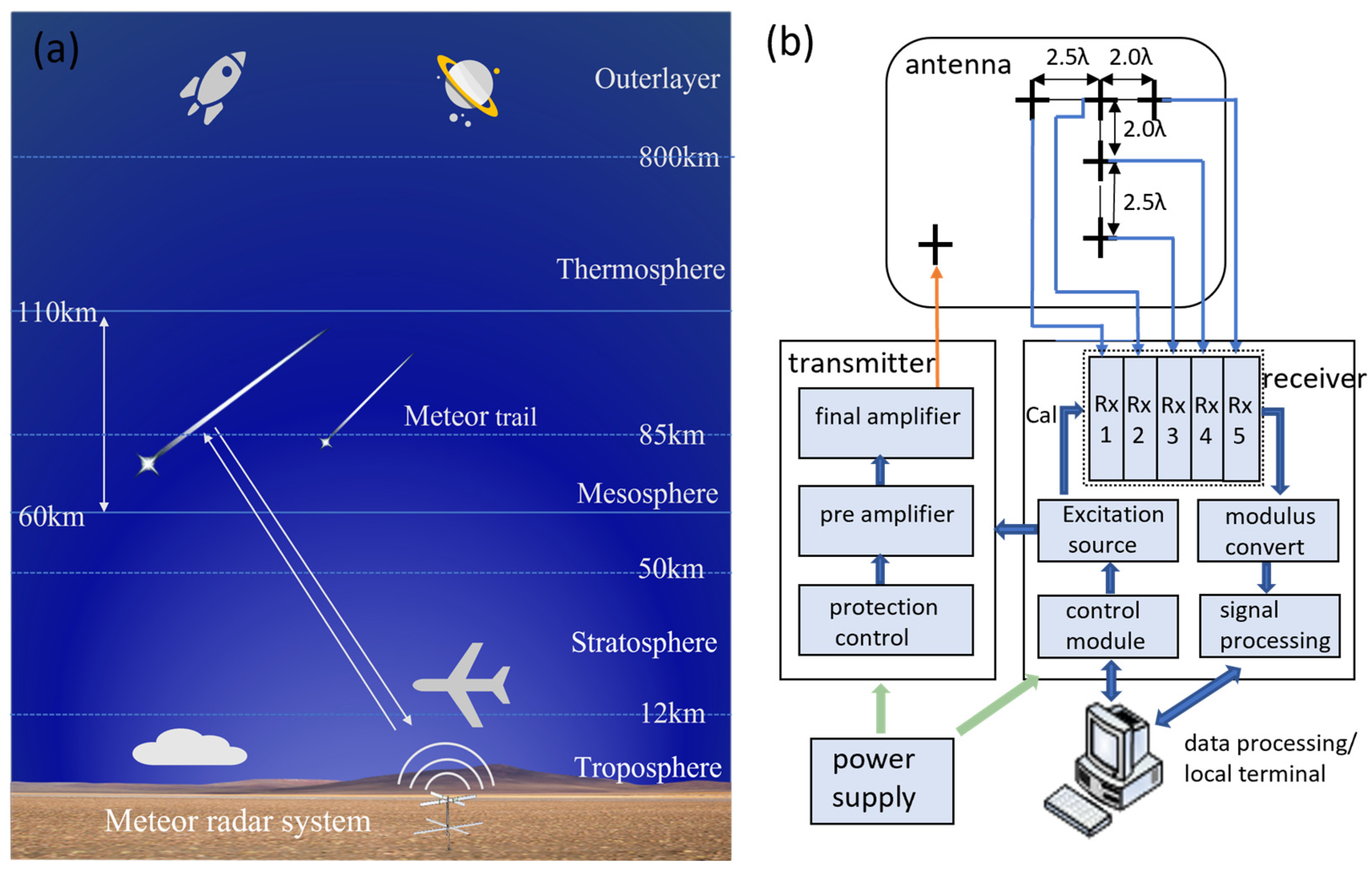
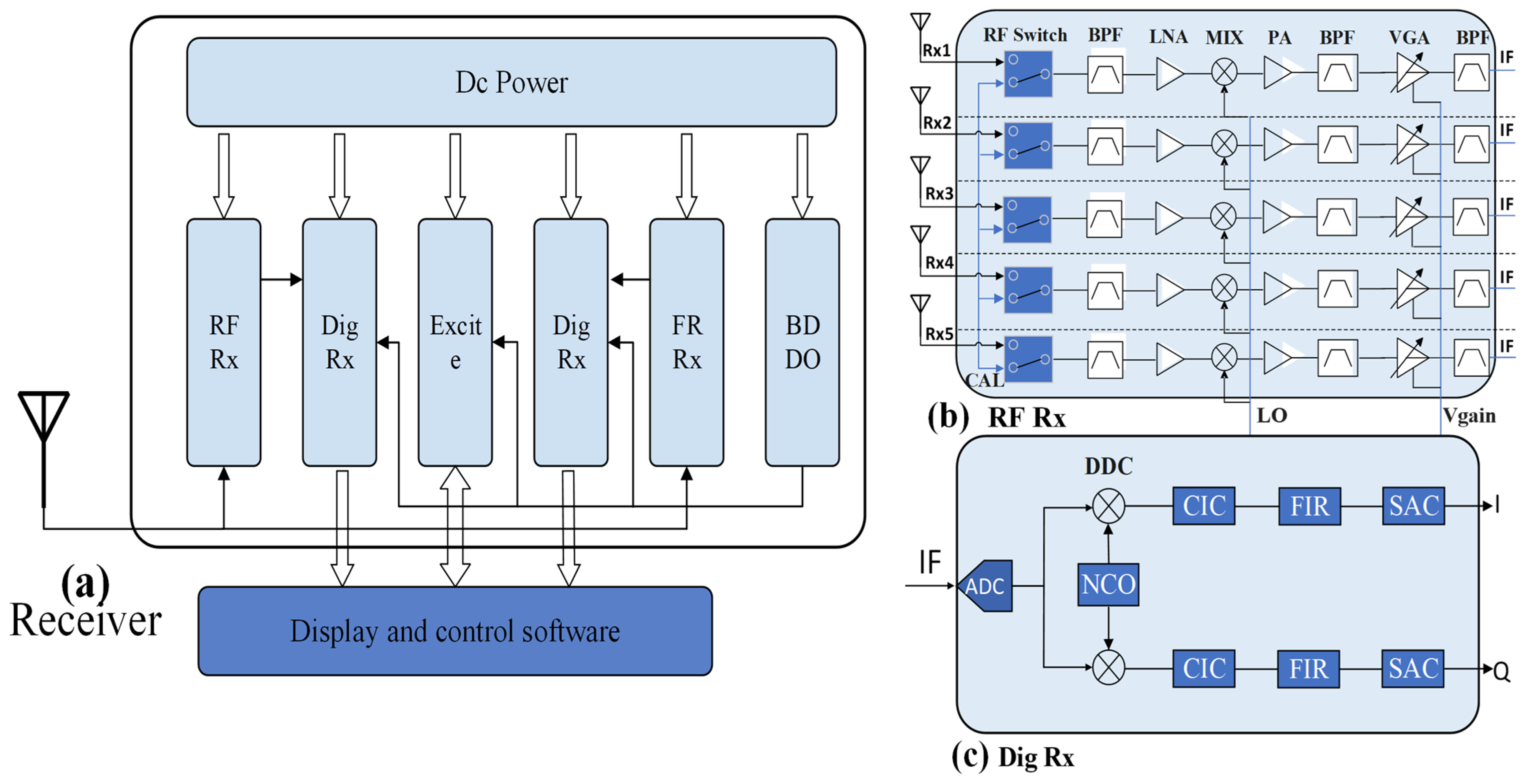
2.1. System Composition

Figure 1a,b illustrates the concept and functional diagrams of meteor radar systems. Figure 1a illustrates the atmospheric layers and the detection height range of meteor radar systems, which primarily encompass the MLT. These radar systems detect backscatter from meteor trails at altitudes between 60 and 110 km, where meteoroids typically appear with a line-of-sight detection range extending beyond 320 km [36]. Unlike conventional narrow-beam radar, the all-sky interferometric meteor radar system utilizes an interferometric method to capture not only components aligned with the Doppler radar beam but also to retrieve the full vector wind field over time. This enhanced capability significantly increases the system’s utility, making it a valuable tool for atmospheric and environmental research [37]. The system detects meteors by transmitting radio waves, which are reflected to the receiver by the plasma column formed from the ionization of air caused by meteors. When the electron line density of the meteor trail is less than 2 × 10¹⁴ m⁻¹, secondary scattering of radio waves can be neglected; such meteors are defined as underdense meteors, which are the primary detection and research targets of this system. Since meteor trails are influenced by both atmospheric horizontal winds and the motion of the meteoroid, variations in the atmospheric wind field can be calculated based on these trails. The ideal underdense meteor echo scattering equation is given as follows:

$$P_R={\displaystyle \frac{P_T{G}_T{G}_R{\lambda }^3{q}^3{r}_e^3\left(C^2+S^2\right)}{64{\pi }^2{R}_0^3}}$$

(1)

where $P_T$ is the radar’s transmitted power, which is 20 kW; $G_T$ and $G_R$ represent the gain of the transmitting and receiving antennas, respectively, $G_T\approx G_R\approx 1$; $\lambda$ is the wavelength of the electromagnetic wave; $q$ represents the electron line density of the meteor trail; $r_e$ is the classical electron radius, with a standard value of 2.8 × 10⁻¹⁵ m; $R_0$ is the straight-line distance from the antenna to the meteor trail, and $C$ and $S$ are Fresnel integrals, $C^2+S^2=4.379$. By substituting a frequency of 39 MHz, when the echo distance is 300 km, the signal echo power is approximately equal to −93.87 dBm.

Figure 1b shows a detailed functional diagram of the all-sky interferometric meteor radar system, which includes a transmitter, a receiver, a data processing terminal, and an outdoor T-shaped interferometric antenna array. According to preset coding types and operating modes in the control module, the system transmits excitation signal waves into the atmosphere through the transmitter and transmitting antenna. When the five receiving antennas in the interferometric array capture echoes from meteor trails, the signals are sent to five reception channels (Rx1 to Rx5) of the receiver, processed through radio frequency modules, analog-to-digital (AD) converters, and digital signal processing units. Processed signals are forwarded to the data processing software on the host computer, which computes meteor information and wind field data. Power is supplied to both the transmitter and receiver, ensuring continuous detection.

The T-shaped interferometric antenna array is composed of two-element Yagi antennas, which includes a single transmitting antenna with orthogonal linear polarization and five receiving antennas with cross-circular polarization. The receiving antennas are arranged such that the x-axis sequentially denotes Rx1, Rx2, and Rx5, while the y-axis represents Rx2, Rx4, and Rx3. The distances between Rx1 and Rx2, as well as between Rx4 and Rx3, are 2.5 λ. The distances between Rx2 and Rx5, and between Rx2 and Rx4, are 2.0 λ. Given that the echo from meteor trails originates from a distant location, the arriving waves are parallel to the receiving antenna array. The arrival angle along the x-axis baseline direction is denoted as ${\beta }_1$, and the arrival angle along the y-axis baseline direction is denoted as ${\beta }_2$. Based on the distances between three antennas along the x-axis and y-axis, as well as the echo phase differences, ${\beta }_1$ and ${\beta }_2$ can be calculated.

The y-axis is aligned northward, and the angle between the meteor echo and the north direction on the horizontal plane is defined as the azimuth angle ($\theta$). The angle between the meteor echo and the horizontal plane is referred to as the elevation angle (φ). Utilizing the spatial relationship between the antenna array and the incoming echo, both the azimuth and elevation angle of the meteor trail echoes can be further computed. These angles are essential for accurately determining the spatial position of meteors. The specific formulas are presented below:

$$\left\{\begin{array}{c}cos{\beta }_1=sin\varphi \times cos\theta \\ cos{\beta }_2=cos\varphi \times cos\theta \end{array}\right.\Rightarrow \left\{\begin{array}{l}\varphi =\mathrm{atan}\left({\displaystyle \frac{\mathit{cos}{\beta }_1}{\mathit{cos}{\beta }_2}}\right)\\ \theta =acos\sqrt{{cos}^2{\beta }_1+{cos}^2{\beta }_2}\end{array}\right.$$

(2)

The accuracy of arrival angle calculations in meteor radar systems is closely tied to the echo phase differences between receiving antennas. Variations in the amplitude and phase characteristics of the receiving antennas, feeder cables, and the receiver’s internal channels introduce errors in the computation of arrival angles, subsequently impacting the precision of the $\theta$ and $\varphi$ angles. Environmental factors such as temperature fluctuations, power supply variations, and component aging further exacerbate these amplitude and phase inconsistencies. In this study, the temperature fluctuations at the meteor radar station are relatively minimal, and the calibration coefficients for the receiving antennas and feeder cables remain fixed and then addressed during post-processing. However, calibrating the internal channels of the meteor radar receiver is significantly more complex and critical. The receiver comprises numerous discrete components, including amplifiers, filters, mixers, radio frequency (RF) switches, power modules, and transmission lines. Variations in these components, influenced by operational conditions, temperature changes, thermal noise, and nonlinear effects, result in intricate amplitude and phase discrepancies between channels. These discrepancies necessitate dynamic calibration adjustments to maintain accuracy.

2.2. Calibration Hardware Circuit Design

In this paper, we propose a comprehensive approach to accomplish the dynamic adaptive calibration of amplitude and phase consistency in meteor radar systems, integrating hardware circuit design and dynamic adaptive calibration algorithm based on NLMS and correlation algorithms. The design of the hardware circuitry forms the foundation of the dynamic adaptive calibration method and incorporates voltage gain control (VGC) adjustments and high-precision clock synchronization across each channel [38,39].

Figure 2a presents the schematic diagram of the meteor radar receiver, which consists of components such as the direct current (DC) power supply and Beidou disciplined oscillator (BDDO), radio frequency receiver (RF Rx), excite and digital receiver (Dig Rx) units. The DC Power unit supplies DC + 5.5 V for each circuit in the receiver. The BDDO unit provides precise timing and clock signals to the main control and data acquisition units, serving as the system’s time and frequency synchronization reference. The Excite unit manages the system’s operating sequence, transmits excitation pulse waveforms, and provides local oscillator (LO) signals and VGC. Its core architecture comprises field programmable gate array (FPGA) and digital-to-analog (DA) modules. The LO signal, VGC, and excitation signal from the Excite unit and the analog-to-digital (AD) chip of the Dig Rx unit share the same clock source. Synchronization settings via the SYNC function between chips ensure initial amplitude and phase consistency accuracy pivotal role in measuring phase consistency across the LO signal, excitation signal, and each receiving channel. The RF Rx unit processes meteor echo signals received by the antennas, performing frequency conversion and filtering before sending the intermediate frequency (IF) signal to the Dig Rx unit for AD acquisition and digital signal processing.

Figure 2b illustrates the block diagram of the RF Rx unit’s five channels reception principle. During the work mode, the RF switch gates the echo signals, and the Excite unit transmits excitation signals to the transmitter, which radiates them through the transmitting antenna. The receiving antenna captures echo signals across five channels, which are processed through the RF Rx units, involving a pre-selection filter, low-noise amplifier, mixing, power amplification, band-pass filtering, and programmable amplification [40]. In the VGC programmable amplification circuit, the hardware design addresses static amplitude discrepancies by calibrating the output amplitude across channels. The amplification factors for each channel are finely tuned using amplifiers and high-precision potentiometer-driven feedback mechanisms, ensuring consistent IF signal amplitudes across all five channels and achieving effective static calibration.

Figure 2c presents the digital signal processing flow within Dig Rx. The IF signal enters the Dig Rx unit for AD acquisition, is converted into two orthogonal in-phase (I) and quadrature phase (Q) baseband signals, and then undergoes digital down conversion (DDC) and cascaded integrator comb (CIC) decimation in the FPGA, reducing the sampling rate from 120 Mbps to 3 Mbps. Next, the data will be processed using finite impulse response (FIR) filtering and spectral amplitude coding (SAC) techniques. Finally, the data are transmitted to the display and control software via the network interface for adaptive algorithm calibration. In calibration mode, the RF switch gates a calibration signal, which is coupled from the excitation signal, attenuated to a lower power than the normal transmission signal, and delayed to simulate an echo after traveling a specific distance. This calibration signal is processed through the receiver’s five channels, RF Rx units, and Dig Rx units, and the data are uploaded to the upper computer software. Initial calibration coefficients are calculated from these data and serve as initial parameters for the calibration algorithm. The algorithm iteratively adjusts these coefficients to obtain the optimal values for that period. After calibration, the system switches to work mode, applying the calibrated coefficients to each channel’s echo signals to maintain dynamic amplitude and phase consistency.

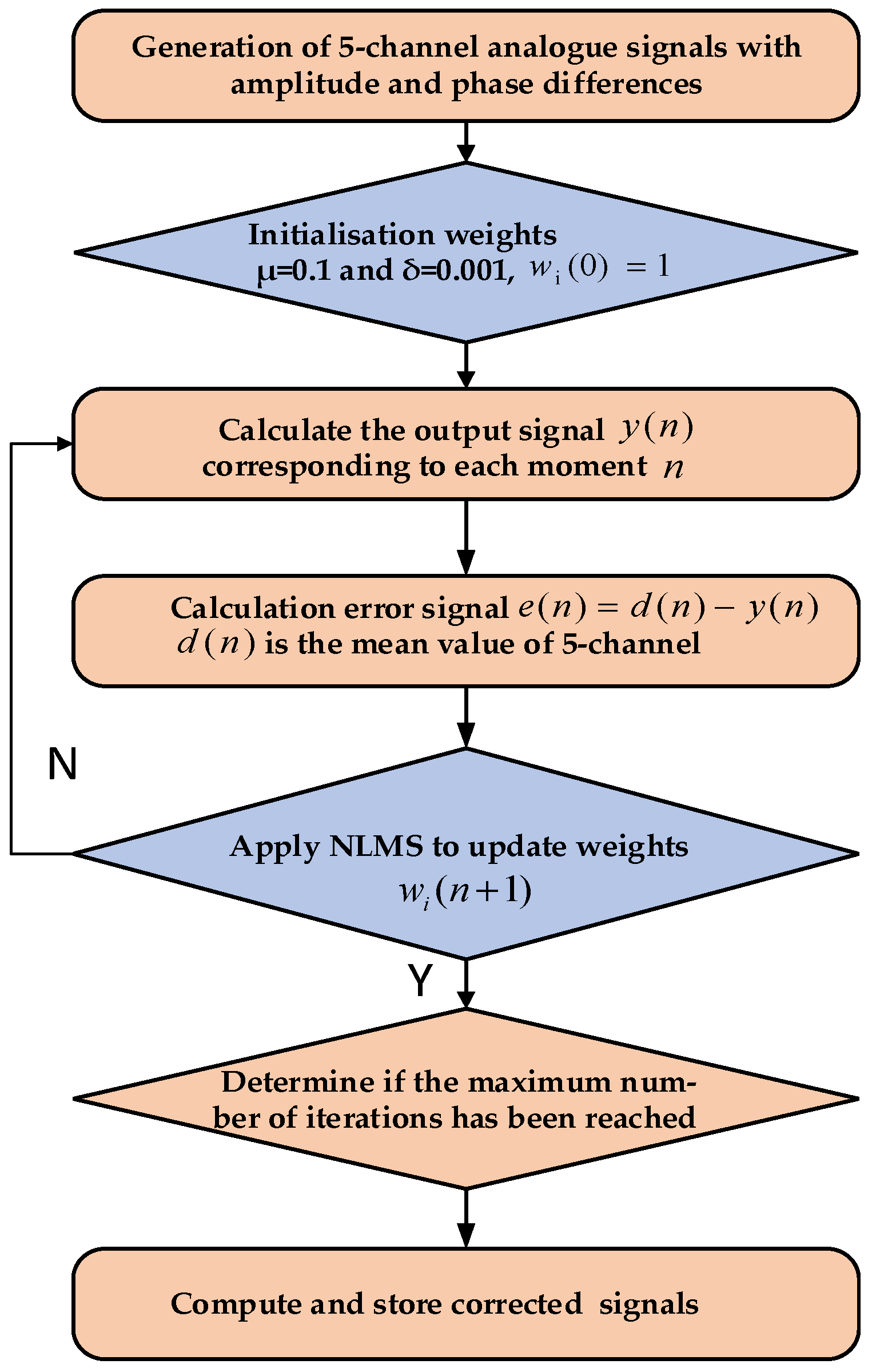
2.3. NLMS and Correlation Calibration Algorithms

The NLMS algorithm is an iterative adaptive filtering technique derived from the basic LMS algorithm, utilizing instantaneous error calculations instead of mean square error (MSE) estimates. Through gradient descent, it iteratively updates filter weights in the direction of the negative gradient of the instantaneous signal error, minimizing the MSE between the input signal and the desired output. While the LMS algorithm is simple and easy to implement, its fixed step size often results in slow convergence, limited adaptability, high sensitivity to step size especially with highly correlated signals, and reduced adaptability in scenarios with frequent signal power fluctuations. Additionally, selecting an optimal step size is challenging, a large step size may cause instability, while a small one slows convergence substantially [41].

The NLMS algorithm addresses these limitations by normalizing the input signal’s power, enabling dynamic adjustment of the step size in response to signal power changes, and allowing more efficient weight updates during processing. The key innovation in NLMS is normalizing the step size by the input signal’s power, which enhances algorithm stability and performance without requiring prior knowledge of the input or desired signal statistics, making it well-suited for real-time applications. Compared to LMS, NLMS achieves significantly faster convergence in fluctuating environments while maintaining high accuracy by adapting the step size, which is particularly effective for signals with large power variations and strong correlations. Despite its slightly higher computational cost from the normalization step, this is offset by its substantial performance gains. With improved adaptability and stability, NLMS is highly applicable to channel equalization, noise cancelation, linear prediction, and system identification, where efficient and precise processing of complex signals is essential [42]. Consequently, NLMS demonstrates superior adaptability and stability in real-time applications, especially for handling dynamically varying and complex signals.

In the all-sky interferometric meteor radar system, dynamic variations in amplitude and phase differences require an algorithm like NLMS, which is well-suited for long-term calibration of the system. The goal of calibration in the meteor radar system is to minimize the MSE between the observed output signal and the desired output by adjusting the phase weights of each channel. This enables the outputs from each channel to achieve a nearly consistent amplitude and phase alignment during calibration mode. In practice, the mean value of the five-channel outputs is typically used as the reference or desired output for calibration.

In the meteor radar system, the input signals from the five channels are denoted as $x_i\left(n\right),i=1,2\dots 5$, where $n$ represents the time index. The desired output signal is denoted as $d\left(n\right)$, which is taken as the mean of the outputs from all channels. The calibration process involves adjusting the weights of each channel to minimize the MSE between the output signal $y\left(n\right)$ and the desired output $d\left(n\right)$. In practical applications, the mean value of 5 channels is defined as the desired output.

The output of the five channels can be expressed as follows:

$$y_i\left(n\right)=\sum _{i=1}^5{w_i}^T\left(n\right)\times x_i\left(n\right)$$

(3)

where $w_i\left(n\right)$ denotes the adjustable weight for the channel $i$ at time $n$. The NLMS algorithm computes the estimated error $e\left(n\right)$ as the difference between the desired output $d\left(n\right)$ and the filter’s actual output $y\left(n\right)$:

$$e\left(n\right)=d\left(n\right)-y\left(n\right)$$

(4)

This error represents the deviation from the desired response, which the algorithm aims to minimize by updating the filter weights.

The MSE $J\left(n\right)$ between the desired output and the actual output is represented as follows:

$$J\left(n\right)=E\left[{\left(d\left(n\right)-y\left(n\right)\right)}^2\right]=E\left[{\left(mean(x_i\left(n\right)-y(n\right))}^2\right]$$

(5)

To minimize $J\left(n\right)$, we apply the NLMS algorithm for calibration of meteor signal power dynamically varies, as it includes a normalization factor that improves stability and convergence speed.

The weight update rule for NLMS incorporates a normalization term that adjusts the learning rate based on the input signal’s energy, which enhances convergence stability under variable input power conditions, the formula is given below:

$$w_i\left(n+1\right)=w_i\left(n\right)+{\displaystyle \frac{\mu \cdot e\left(n\right)\cdot x_i\left(n\right)}{{‖x\left(n\right)‖}^2+\delta }}$$

(6)

where $\mu$ is the step size parameter controlling the adaptation rate, the initial value can be set to $0<\mu <2$ for stability. The $w_i\left(0\right)$ commonly is initialized to zero; however, a more reasonable initial value for this parameter is obtained through the correlation algorithm in this paper.

$${‖x\left(n\right)‖}^2={\sum }_{i=1}^5{x}_i{\left(n\right)}^2$$

(7)

${‖x\left(n\right)‖}^2$ denotes the squared norm of the input signal, and $\delta$ is a small positive constant added to avoid division by zero.

The NLMS algorithm thus iteratively optimizes each weight $w_i\left(n\right)$ to ensure that the combined output $y\left(n\right)$ aligns closely with the desired output $d\left(n\right)$. This algorithmic modification helps stabilize the calibration under fluctuating input conditions, which is essential for meteor radar systems operating under varying signal environments.

In practical applications of amplitude and phase consistency calibration for all-sky interferometric meteor radar systems, it is essential to select appropriate step sizes and stopping conditions based on specific situations and hardware conditions, and to fine-tune parameters to enhance algorithm performance. The NLMS algorithm effectively resolves this problem.

During the calibration mode of the meteor radar system, the calibration signal is imported to all five channels. This signal is derived from the excitation signal and fed into each channel through a power splitter, with its power attenuated to approximately −70 dBm and a delay set of 600 µs. Considering the speed of electromagnetic wave propagation, this delay corresponds to a meteor echo distance calculated as $d=c\ast {\displaystyle \frac{t}{2}}$. Where $d$ is the distance, $c$ is the speed of light, and $t$ is the time delay. The calculated distance is approximately 90 km, which lies within the system’s detection range. In calibration mode, the receiver acquires the calibration signal across five channels. If the amplitude and phase coefficient of the five channels are consistent, each channel should output signals with the same amplitude and phase. The mean output across the five channels is used as the reference signal. Amplitude and phase discrepancies are corrected by comparing each channel’s output to this reference. These weights are updated using the NLMS algorithm to derive the dynamic optimal calibration coefficients during calibration mode. These coefficients are then applied in operational mode to calibrate amplitude and phase consistency in the collected five-channel waveform.

In application of the NLMS algorithm, initial weights are typically set to zero, or to empirical or measured values to simplify the implementation. The initial weight settings affect both the convergence rate and algorithm performance, potentially delaying the calibration process for achieving the desired output. In this paper, the initial weight settings in the NLMS algorithm for meteor radar are investigated, and an innovative adaptive calibration algorithm is proposed combining the sliding correlation algorithm and NLMS for amplitude and phase consistency [43]. By employing sliding correlation to find the coordinates of the maximum signal energy of the echo waveform, precise initial calibration coefficients are calculated for the NLMS calibration algorithm. Both the adaptive step and precise initial weight effectively enhance the convergence rate and algorithm performance of the NLMS algorithm. The specific implementation steps are as follows:

• Collect one second of echo data to obtain the raw I/Q waveform data of the A and B codes (complementary code sequences) for the five channels;
• Under the condition of a pulse repetition frequency of 430 Hz, extract 6000 data points;
• Perform a sliding correlation algorithm on the extracted data. The sliding window $W_L=N_L=430$ and sliding correlation calculation formula is as follows:

  $$\mathrm{Xcorr}(i)=\sum _{k=1}^{W_L}[R_I(i,k)+j{R}_Q(i,k)]\times [A_I(i,k)+j{A}_Q(i,k)]$$

  (8)

Search for the maximum value of the correlation peak after the sliding correlation, which is the calibration reference point of the radar echo signal. In this equation, R represents the received complex signal and A denotes the reference complex signal for calibration.

4.

Calculate the amplitude and phase values of the echo signals $C{H}_i\left(n_{max}\right)$ corresponding to each channel point index $n_{max}$;

5.

Use the mean value of five channels as the calibration reference and calculate the initial amplitude and phase calibration coefficient $w_{\mathrm{i}}\left(0\right)$ for each channel at $n_{max}$;

$$w_i\left(0\right)={\displaystyle \frac{{CH}_i\left(n_{max}\right)}{{mean(CH}_i\left(n_{max}\right))}}{=A}_{\mathrm{cal}}\left(i,0\right)+j{P}_{\mathrm{cal}}\left(i,0\right)$$

(9)

$A_{\mathrm{cal}}\left(i,0\right)$ and $P_{\mathrm{cal}}\left(i,0\right)$ represent the amplitude and phase calibration initial coefficients, respectively.

6.

Set the initial value of step-size $\mu =0.1$ and $\delta =0.001$;

7.

Obtain the current input signal $x\left(n\right)$;

8.

Compute the filter output $y\left(n\right)$ as Formula (3);

9.

Calculate the error as Formula (4), the target value is $e\left(n\right)=0.01+j0.01$;

10.

Update the weights $w_i\left(n+1\right)$ of each channel according to the NLMS algorithm as Formula (6);

11.

Set the maximum number of iterations to 1000;

12.

Repeat steps 7 to 10 until the error criterion is met or the maximum number of iterations is reached;

13.

For the received five channels of meteor data, perform the calibration by multiplying the complex calibration coefficients, and separately calculate the I and Q signals for each channel. The formula below shows the calibration coefficients obtained through the NLMS algorithm for each channel;

$$y_i\left(n\right)=w_i\left(n\right)\times {CH}_i\left(n\right)=\left(A_{cal}\left(i,n\right)+jC\mathrm{al}\left(i,n\right)\right)\times \left(R_I\left(i,n\right)+j{R}_Q\left(i,n\right)\right)$$

(10)

In the calibration process, selecting an appropriate step size is critical for balancing convergence speed and overall performance. If the learning rate is too high, the algorithm may oscillate or diverge during its search for an optimal solution. Conversely, if the learning rate is too low, the convergence speed will be significantly reduced, requiring more iterations to reach the desired threshold, which can negatively impact the system’s operational efficiency. Therefore, setting appropriate stopping conditions is essential. In this paper, reasonable target thresholds and maximum iterations are established to ensure the computational efficiency and practical performance of the dynamic adaptive calibration algorithm.

3. Simulation

The dynamic adaptive calibration algorithm is implemented using simulation software. The specific steps for the simulation are presented in Figure 3 as follows. Initially, five channels of radar signals are generated, with each channel incorporating random amplitude and phase noise. This results in signals with amplitude and phase discrepancies across the channels. To achieve consistent amplitude and phase alignment, the NLMS adaptive algorithm is employed for calibration. Before applying the adaptive calibration algorithm, initial weights and termination conditions are properly configured. The mean signal across the five channels is set as the reference signal. Using the NLMS algorithm, the calibration coefficients are dynamically adjusted to optimize alignment with the reference, ensuring consistency across channels. Once calibration is complete, the calibrated signals of all five channels are stored and processed.

By iteratively adjusting the weights of each channel, the algorithm eventually calibrates the amplitude and phase discrepancies across all channels. The iteration process is governed by a termination condition, which can either be the maximum number of iterations or the achievement of a predefined error target threshold. The time and frequency domain waveform before and after calibration are compared to validate the effectiveness of the proposed method. Detailed simulation results are presented in the following figures. Figure 4a shows the time-domain waveform of the simulated five channels of signals, which exhibit amplitude and phase discrepancies due to noise. Figure 4b presents the corresponding power spectral density (PSD) plots for each channel, with an amplitude discrepancy of up to ±1.5 dB and a phase variation of up to ±27°. These figures clearly demonstrate significant amplitude and phase discrepancies among the five channels. After applying the NLMS adaptive algorithm and correlation algorithm, the signals show remarkable improvement.

Figure 4c,d illustrate the time-domain waveforms and PSD plots of the signals post-correction, respectively. The nearly identical and overlapping waveforms across all five channels confirm the significant improvements in amplitude and phase consistency achieved by the NLMS adaptive algorithm in both the time and frequency domains. This algorithm effectively calibrates amplitude and phase discrepancies, ensuring consistent signal integrity across all channels. In summary, the simulation results validate both theoretical feasibility and practical effectiveness of the proposed calibration algorithm [44].

4. Application in Meteor Radar

In this paper, we conduct dynamic adaptive calibration experiments to assess the practical effectiveness of the proposed method. The calibration experiments include a comparison of meteor echo images generated by the display and control software, signal waveforms, and pulse compression data analysis, both of which demonstrate the algorithm’s calibration performance and effect on the meteor radar system. All calibration experiment data are real meteor radar system data.

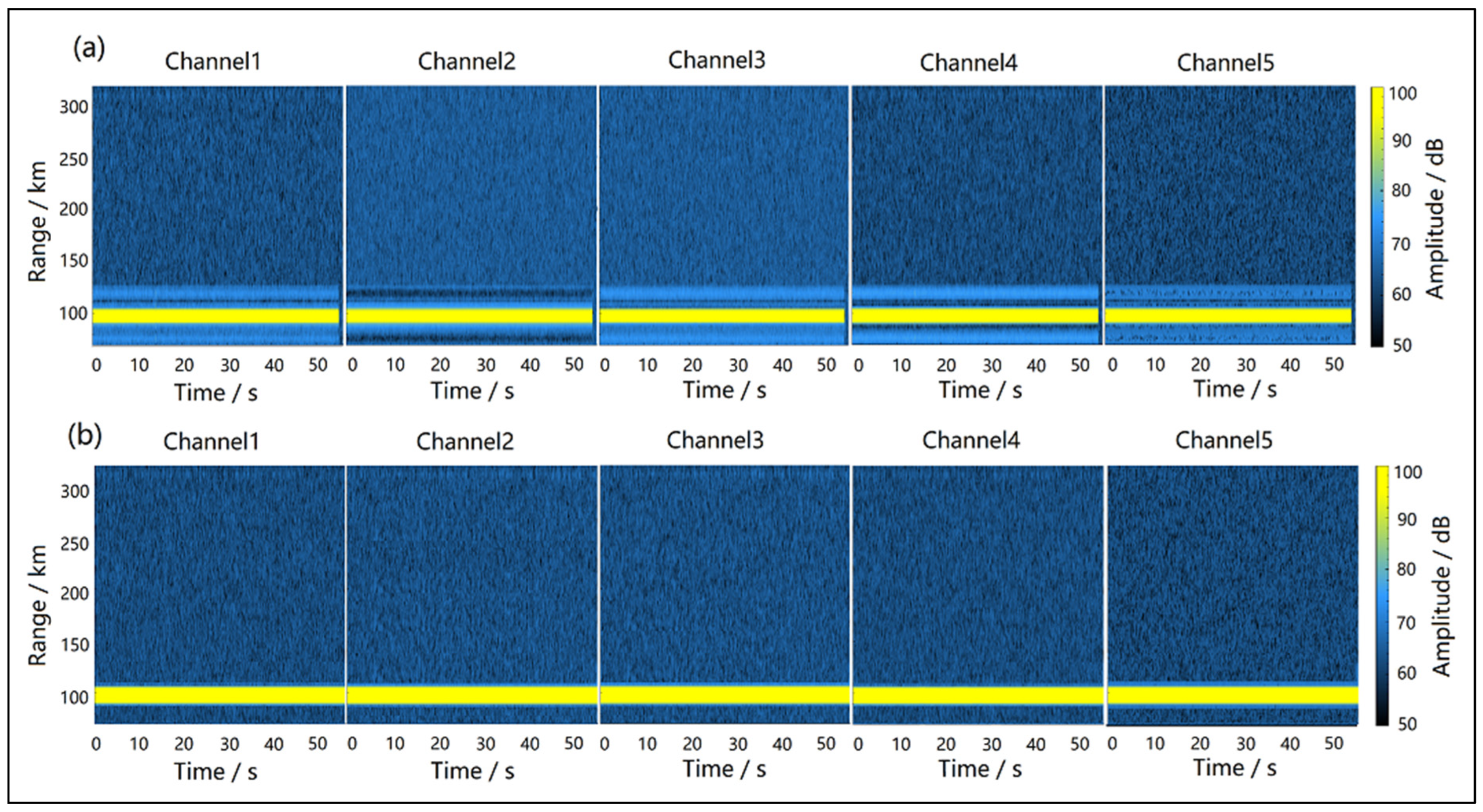
4.1. Calibration Effect on Meteor Echo Image

The meteor echo graphs received from the receiver’s five channels can be observed by using the display and control software of the radar system. In the normal work mode, the echo graphs update every minute. Figure 5a,b presents the meteor echo image before and after the adaptive calibration algorithm, respectively. Channel 1 to channel 5 correspond to the five receiving channels. The horizontal axis represents the echo time within each minute, with an echo collection time of 56 s per cycle. The vertical axis indicates the straight-line distance of the echo signal, ranging from 0 to 320 km, and the color bar on the right corresponds to the echo signal strength. The yellow band at the 90 km mark represents the calibration signal received across all five channels.

Comparing the meteor echo graphs before and after applying the adaptive calibration algorithm, Figure 5a shows the five channels’ echo signals without the NLMS and correlation adaptive calibration algorithm. The yellow echo signal band appears dimmer, with noticeable clutter interference on both sides, and significant color and interference differences among the channels. In contrast, Figure 5b representing the calibration results, shows a brighter yellow signal band, an improved signal-to-noise ratio (SNR), reduced clutter interference, and enhanced channel consistency. The comparison indicates that the amplitude and phase consistency calibration algorithm substantially improve the consistency of the echo signal waveforms across the channels.

4.2. Calibration Effect on Pulse Compression

In the work mode of the meteor radar system, after completing the echo RF signal processing and digital signal processing, the receiver performs amplitude and phase consistency calibration, followed by pulse compression, using the software. The wide pulse complementary code signals undergo autocorrelation processing and are compressed into narrow pulse signals. This process enhances the SNR and detection resolution while preserving the radar system’s detection range. Figure 6a,b illustrates a significant improvement in the amplitude and phase consistency of the five channels of pulse compression waveform after calibration.

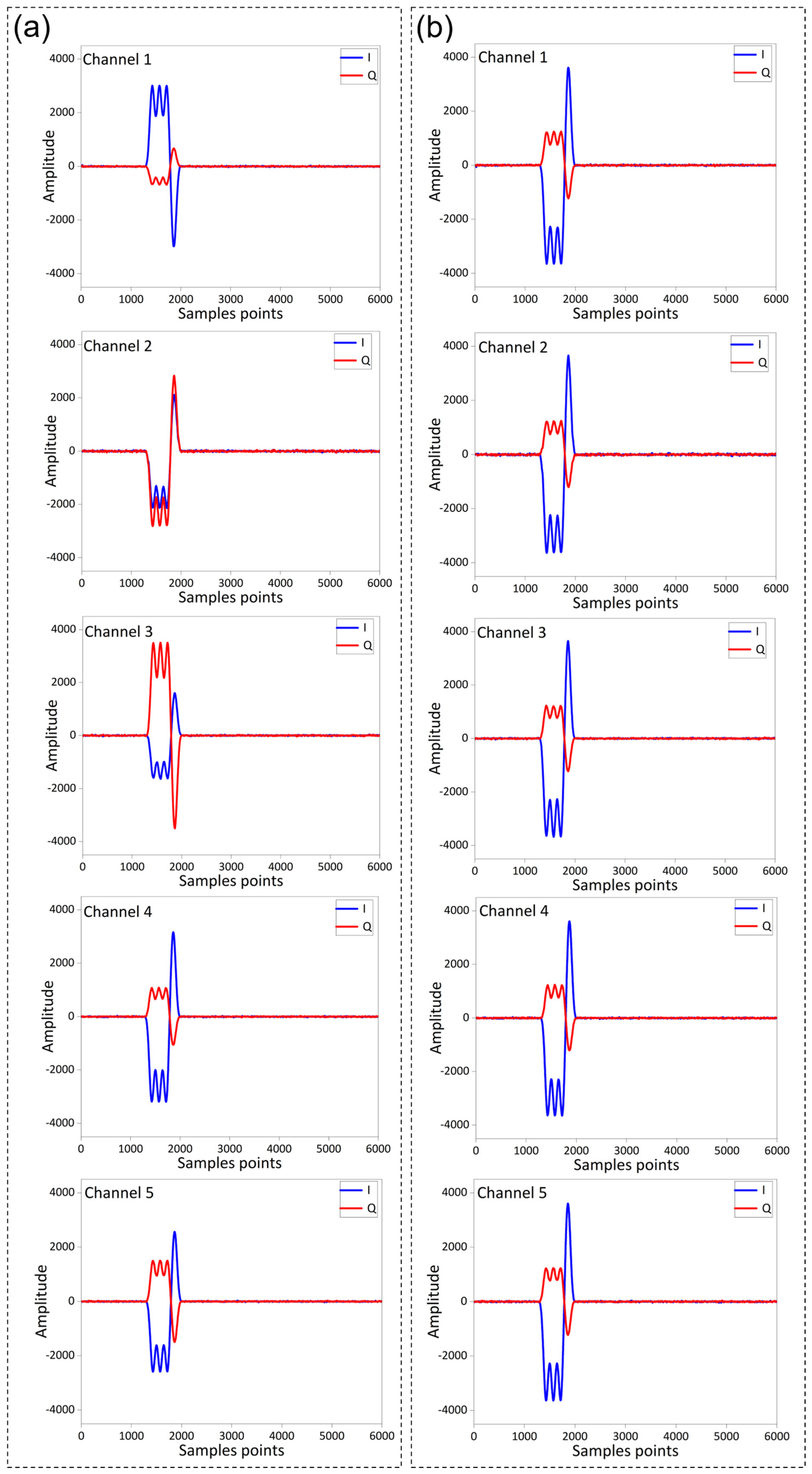
4.3. Calibration Effect on Signal Waveforms

In this calibration experiment, the I/Q signal waveforms processed by the Dig Rx unit were analyzed before and after calibration. Figure 7a,b illustrates the I/Q signal waveforms for all five channels, shown before and after calibration, respectively. In these figures, the blue curve represents the I signal, while the red curve corresponds to the Q signal. The horizontal axis denotes the number of sampling points, and the vertical axis indicates the relative amplitude of the sampled signals. Figure 7a reveals significant discrepancies in signal amplitude and phase among the channels. After calibration, as shown in Figure 7b, these amplitude and phase discrepancies in the I/Q signals across the five channels are substantially reduced. Moreover, the I/Q signal waveforms across the five channels display a high degree of consistency.

To precisely calculate and analyze the amplitude and phase consistency, before and after the calibration mode of the meteor radar system, four points of signal code element data were collected to calculate the amplitude and phase of the five channels waveform. In practice, the power and phase values were obtained near the maximum peak of the I/Q data, with the following specific formula. Because small values of I/Q data are typically noise and do not accurately reflect the true effect of the calibration, they are excluded from the analysis. This approach ensures that the evaluation of the calibration process is based on meaningful data that accurately represents the system’s performance improvements.

$$\theta \left(i,n_p\right)={\mathit{tan}}^{-1}\left[{\displaystyle \frac{R_I\left(i,n_p\right)}{R_Q\left(i,n_p\right)}}\right]\times {\displaystyle \frac{180}{\pi }}$$

(11)

$$P_{dbm}\left(i,n_p\right)=10\times \mathit{lg}\left[{\displaystyle \frac{{R_I\left(i,n_p\right)}^2+{R_Q\left(i,n_p\right)}^2}{50}}\times {\displaystyle \frac{1000}{2}}\right]$$

(12)

Equations (11) and (12) describe the computation of the phase and power of an I/Q signal. The phase ${\theta }_{\left(i,n_p\right)}$ is determined by taking the arctangent of the ratio between the in-phase $\left(R_I\left(i,n_p\right)\right)$ and quadrature $\left(R_I\left(i,n_p\right)\right)$ components of the signal. Here, the result is converted from radians to degrees to facilitate practical interpretation. In Equation (12), the power $P_{dbm}\left(i,n_p\right)$ is computed by summing the squared magnitudes of the I/Q components, dividing the sum by the load resistance (50 ohms), and scaling the result by a factor of 1000/2 to account for the conversion to milliwatts. The logarithmic transformation is then applied to express the power in decibels relative to one milliwatt (dBm). These calculations provide an accurate characterization of the phase and power of the I/Q signal, which is essential for signal analysis in radar and communication systems.

Based on the above formulas, the amplitude and phase values of four data points across five channels are calculated. Subsequently, the standard deviation of the amplitude and phase data for each channel is computed, providing quantitative results for amplitude and phase consistency.

Table 1. Contrast of amplitude and phase calibration results.

Channel		Amplitude (dB)				Phase (o)
		Point1	Point 2	Point 3	Point 4	Point 1	Point 2	Point 3	Point 4
Original	CH1	−0.9784	−0.9932	−1.0822	−1.0515	−86.9761	−91.5301	91.7915	−86.6542
	CH2	−1.8672	−1.8479	−1.9218	−1.9057	−90.3839	−94.9626	88.1729	−90.4200
	CH3	−0.8439	−0.7950	−0.9011	−0.8842	−88.7715	−93.1451	89.9926	−88.6469
	CH4	−1.2654	−1.2765	−1.3215	−1.3042	−77.7208	−82.4398	100.8693	−77.5637
	CH5	−0.3864	−0.3812	−0.4660	−0.4582	−73.5094	−77.8493	105.2076	−73.3297
	Consistency	0.4900	0.4905	0.4815	0.4795	6.6403	6.6538	6.6394	6.6760
Calibrated	CH1	−2.7473	−2.7621	2.8512	−2.8205	−90.4151	−94.9691	88.3525	−90.0932
	CH2	−2.7823	−2.763	−2.8369	−2.8208	−90.3839	−94.9626	88.1729	−90.4200
	CH3	−2.7701	−2.7212	−2.8273	−2.8104	−90.7171	−95.0908	88.0470	−90.5926
	CH4	−2.7610	−2.7721	−2.8171	−2.7998	−90.2123	−94.9312	88.3779	−90.0552
	CH5	−2.7499	−2.7448	−2.8295	−2.8217	−90.3544	−94.6943	88.3626	−90.1747
	Consistency	0.0141	0.0173	0.0113	0.0085	0.1655	0.1296	0.1311	0.2064

presents the computed calibration results for the five channels, providing a detailed comparison of amplitude and phase consistency before and after applying the calibration algorithm. The amplitude consistency across the five channels before calibration ranged from 0.4795 dB to 0.4905 dB, indicating significant discrepancies in signal amplitude among the channels. After calibration, the amplitude consistencies were reduced to a range of 0.0085 dB to 0.0173 dB, demonstrating remarkable improvement. Regarding phase consistency, the original phase consistency before calibration ranged from 6.6394° to 6.6760°, highlighting considerable phase differences among the channels. After calibration, the phase consistency was significantly reduced, falling within a much narrower range of 0.1296° to 0.2064°.

5. Discussion

Table 1 presents a comparison of amplitude and phase consistencies between raw and calibrated signals. The results demonstrate a significant improvement in amplitude and phase consistencies after calibration, validating the effectiveness of the NLMS calibration algorithm. To further assess the reliability and validity of the NLMS dynamic calibration method against the conventional static calibration method, as well as to validate the dynamic variations in amplitude and phase consistencies of the meteor radar system, comparative and repeated calibration tests are essential.

In this study, calibration tests were conducted on a meteor radar system under consistent operational modes and time settings. In the NLMS dynamic calibration method, calibration coefficients were updated dynamically, while in the static method, coefficients remained fixed throughout the tests. Calibration sessions were scheduled every two hours, with multiple data collection periods for thorough analysis. Figure 8a,b show the amplitude and phase consistency diagrams of the radar over 48 h before calibration.

Apparently, both the amplitude consistency and phase consistency exhibit dynamic variation.

Next, the results of amplitude and phase consistency after calibration are analyzed. For each calibration operation, the amplitude and phase consistency results of four data points for five channels are analyzed and calculated before and after calibration. Six sets of correction results were collected and computed for each method, with the test results are shown in Figure 9, providing an intuitive representation of the six calibration trials. After NLMS dynamic calibration, as shown in Figure 9a, amplitude consistency is reduced to below 0.0343 dB, while phase consistency decreases to less than 0.2170°, illustrated in Figure 9b.

Comparative experiments were conducted using the conventional static calibration method, where the amplitude and phase consistency calibration coefficients remained fixed. The results are shown in Figure 10a,b. Repeatability tests indicate that, with fixed coefficients, the amplitude consistency after calibration ranges from 0.0163 dB to 0.053 dB, while the phase consistency varies significantly, from 0.2250° to 4.9780°. These findings clearly demonstrate that the NLMS dynamic calibration method provides a substantial improvement in amplitude and phase consistency compared to the static calibration approach.

In the application results of the meteor radar system, the comparison of meteor echo images, pulse compression frequency-domain calibration, I/Q signal waveform calibration and amplitude-phase consistency calculations provide comprehensive validation of the NLMS dynamic calibration method. The comparisons and repeat calibration results strongly affirm the remarkable effectiveness of the proposed method in meteor radar system applications. Furthermore, calibration experiments confirm the dynamic variations in amplitude and phase consistency and comprehensively demonstrate the overall effectiveness of the NLMS dynamic correction method in meteor radar systems. The significant improvement in consistency underscores the critical role of the calibration process in ensuring accurate and reliable signal measurements. Such precision is essential for the high-performance operation of meteor radar systems.

6. Conclusions

In this study, we propose a novel adaptive calibration method to address dynamic amplitude and phase consistency in all-sky meteor radar systems. Our approach integrates theoretical analysis, hardware circuit design, and a dynamic calibration algorithm that combines NLMS and correlation techniques. The system’s hardware mitigates initial amplitude and phase consistency with VGC and high-precision clock synchronization AD acquisition units across all channels. Calibration coefficients are initially determined using correlation algorithms and are then refined in real time via the NLMS algorithm, enabling dynamic updates and optimization of these coefficients.

We demonstrate the effectiveness of our method through rigorous testing on a meteor radar system. Consistent and repeatable results from NLMS-based dynamic calibration show a significant reduction in amplitude and phase discrepancies when compared to traditional static calibration methods. These findings highlight the advantages of real-time dynamic calibration in improving the precision and consistency of amplitude and phase correction, even as dynamic variations occur within the radar system. Furthermore, long-term reproducibility tests validate the stability and reliability of the calibration method, demonstrating its capacity to adapt to ongoing changes in amplitude and phase discrepancies.

By enabling the real-time calculation and adjustment of calibration coefficients, our method significantly enhances the accuracy of amplitude and phase correction, which is critical for optimizing detection accuracy and wind inversion precision in meteor radar systems. These advancements provide valuable tools for the practical deployment of radar systems in meteorological and atmospheric research.

Although the method is specifically tailored for meteor radar systems, its flexibility suggests broader applicability to multi-channel radar systems that require amplitude and phase consistency calibration. The findings from this work have broader implications for radar technology, particularly in advancing real-time calibration capabilities and overall system accuracy. However, the complex noise environments encountered in application environments present challenges to the practical implementation of this calibration approach. Addressing these challenges will be an important direction for future research.

References

1. Hao, X.; Ma, Y.; Ding, Z.; Wang, L.; Li, N.; Chen, J. Influence of Meteor Count on Wind Field Retrieved by All-Sky Meteor Radar. Atmosphere 2023, 14, 519. [Google Scholar] [CrossRef]
2. Younger, J.P.; Reid, I.M.; Vincent, R.A.; Murphy, D.J. A Method for Estimating the Height of a Mesospheric Density Level using Meteor radar. Geophys. Res. Lett. 2015, 42, 6106–6111. [Google Scholar] [CrossRef]
3. Zhou, B.Z.; Xue, X.H.; Yi, W.; Ye, H.L.; Zeng, J.; Chen, J.S.; Wu, J.F.; Chen, T.D.; Dou, X.K. A Comparison of MLT Wind between Meteor Radar Chain Data and SD-WACCM Results. Earth Planet. Phys. 2022, 6, 451–464. [Google Scholar] [CrossRef]
4. Reid, I.M. Meteor Radar for Investigation of the MLT Region: A Review. Atmosphere 2024, 15, 505. [Google Scholar] [CrossRef]
5. Yi, W.; Xue, X.; Chen, J.; Chen, T.; Li, N. Quasi-90-day Oscillation Observed in the MLT Region at Low Latitudes from the Kunming Meteor Radar and SABER. Earth Planet. Phys. 2019, 3, 136–146. [Google Scholar] [CrossRef]
6. Yi, W.; Xue, X.H.; Lu, M.L.; Zeng, J.; Ye, H.L.; Wu, J.F.; Wang, C.; Chen, T.D. Mesopause temperatures and relative densities at midlatitudes observed by the Mengcheng meteor radar. Earth Planet. Phys. 2023, 7, 665–674. [Google Scholar] [CrossRef]
7. Ceplecha, Z.; Borovicka, J.Í.; Elford, W.G.; ReVelle, D.O.; Hawkes, R.L.; Porubcan, V.Í.; Šimek, M. Meteor Phenomena and Bodies. Space Sci. Rev. 1998, 84, 327–471. [Google Scholar] [CrossRef]
8. Jones, J.; Campbell Brown, M. The Initial Train Radius of Sporadic Meteors. Mon. Not. R. Astro. Soc. 2005, 359, 1131–1136. [Google Scholar] [CrossRef]
9. Wang, J.; Yi, W.; Wu, J.; Chen, T.; Xue, X.; Zeng, J.; Vincent, R.A.; Reid, I.M.; Batista, P.P.; Buriti, R.A.; et al. Coordinated observations of migrating tides by multiple meteor radars in the equatorial mesosphere and lower thermosphere. J. Geophys. Res. Space Phys. 2022, 127, e2022JA030678. [Google Scholar] [CrossRef]
10. Hall, C.; Dyrland, M.; Tsutsumi, M.; Mulligan, F. Temperature trends at 90 km over Svalbard, Norway (78°N l6°E), seen in one decade of meteor radar observations. J. Geophys. Res. 2012, 117, D08104. [Google Scholar] [CrossRef]
11. Yi, W.; Xue, X.; Chen, J.; Dou, X.; Chen, T.; Li, N. Estimation of Mesopause Temperatures at Low Latitudes using the Kunming Meteor radar. Radio Sci. 2016, 51, 130–141. [Google Scholar] [CrossRef]
12. Stober, G.; Vadas, S.L.; Becker, E.; Liu, A.; Kozlovsky, A.; Janches, D.; Qiao, Z.; Krochin, W.; Shi, G.; Yi, W.; et al. Gravity waves generated by the Hunga Tonga–Hunga Ha′apai volcanic eruption and their global propagation in the mesosphere/lower thermosphere observed by meteor radars and modeled with the High-Altitude general Mechanistic Circulation Model. Atmos. Chem. Phys. 2024, 24, 4851–4873. [Google Scholar] [CrossRef]
13. He, M.; Forbes, J.M. Rossby wave second harmonic generation observed in the middle atmosphere. Nat. Commun. 2022, 13, 7544. [Google Scholar] [CrossRef] [PubMed]
14. Kam, H.; Kim, Y.H.; Mitchell, N.; Kim, J.-H.; Lee, C. Evaluation of Estimated Mesospheric Temperatures from 11-year Meteor Radar Datasets of King Sejong Station (62°S, 59°W) and Esrange (68°N, 21°E). J. Atmos. Sol.-Terr. Phys. 2019, 196, 105148. [Google Scholar] [CrossRef]
15. Yang, C.; Lai, D.; Yi, W.; Wu, J.; Xue, X.; Li, T.; Chen, T.; Dou, X. Observed Quasi 16-Day Wave by Meteor Radar over 9 Years at Mengcheng (33.4°N, 116.5°E) and Comparison with the Whole Atmosphere Community Climate Model Simulation. Remote Sens. 2023, 15, 830. [Google Scholar] [CrossRef]
16. Batubara, M.; Yamamoto, M.-Y.; Madkour, W.; Manik, T. Long-term distribution of meteors in a solar cycle period observed by VHF meteor radars at near-equatorial latitudes. J. Geophys. Res. Space Phys. 2018, 123, 10403–10415. [Google Scholar] [CrossRef]
17. Holdsworth, D.A.; Reid, I.M.; Cervera, M.A. Buckland Park All-Sky Interferometric Meteor Radar. Radio Sci. 2004, 39, RS5009. [Google Scholar] [CrossRef]
18. Zeng, J.; Stober, G.; Yi, W.; Xue, X.; Zhong, W.; Reid, I.; Adami, C.; Ning, B.; Li, G.; Dou, X. Mesosphere/Lower Thermosphere 3-Dimensional Spatially Resolved Winds observed by Chinese Multistatic Meteor Radar Network using the Newly developed VVP Method. J. Geophys. Res. Atmos. 2024, 129, e2023JD040642. [Google Scholar] [CrossRef]
19. Hocking, W.; Fuller, B.; Vandepeer, B. Real-Time Determination of Meteor-correlation Parameters Utilizing Modern Digital Technology. J. Atmos. Sol.-Terr. Phys. 2001, 63, 155–169. [Google Scholar] [CrossRef]
20. Wang, D.; Zhang, F.; Chen, L.; Li, Z.; Yang, L. The Calibration Method of Multi-Channel Spatially Varying Amplitude-Phase Consistency Errors in Airborne Array TomoSAR. Remote Sens. 2023, 15, 3032. [Google Scholar] [CrossRef]
21. Maghraby, A.K.S.E.; Park, H.; Camps, A.; Grubii, A.; Colombo, C.; Tatnall, A. Phase and baseline calibration for microwave interferometric radiometers using beacons. IEEE Trans. Geosci. Remote Sens. Lett. 2020, 58, 5242–5253. [Google Scholar] [CrossRef]
22. Yi, W.; Xue, X.; Reid, I.; Younger, J.; Chen, J.; Chen, T.; Li, N. Estimation of Mesospheric Densities at Low Latitudes using the Kunming Meteor Radar together with SABER Temperatures. J. Geophys. Res. Space Physics. 2018, 123, 3183–3195. [Google Scholar] [CrossRef]
23. Zhou, Y.; Wang, W.; Chen, Z.; Wang, P.; Zhang, H.; Qiu, J.; Zhao, Q.; Deng, Y.; Zhang, Z.; Yu, W. Digital beamforming synthetic aperture radar (DBSAR): Experiments and performance analysis in support of 16-channel airborne X-band SAR data. IEEE Trans. Geosci. Remote Sens.Lett. 2020, 59, 6784–6798. [Google Scholar] [CrossRef]
24. Meng, Z.; Li, Y.; Song, X.; Xing, M.; Bao, Z. Amplitude-phase Discontinuity Calibration for Phased Array Radar in Varying Gamming Environment. IET Signal Process. 2014, 8, 729–737. [Google Scholar] [CrossRef]
25. Chen, H.; Ming, F.; Li, L.; Liu, G. Elevation Multi-Channel Imbalance Calibration Method of Digital Beamforming Synthetic Aperture Radar. Remote Sens. 2022, 14, 4350. [Google Scholar] [CrossRef]
26. Deng, X.; Lan, A.L.; Yan, J.Y.; Wu, L.; Wu, J.; Zhang, J.J. Calibrating the amplitude and phase imbalances in agiledarn hf radar. Radio Sci. 2021, 56, e2020RS007138. [Google Scholar] [CrossRef]
27. Zhou, Y.; Li, J.; Zhang, H.; Chen, Z.; Zhang, L.; Wang, P. Internal Calibration for Airborne X-Band DBF-SAR Imaging. IEEE Geosci. Remote Sens. Lett. 2021, 19, 1–5. [Google Scholar] [CrossRef]
28. Rousta, B.; Naser-Moghadasi, M.; Arand, B.A.; Sadeghzadeh, R.A. An Efficient Scheduling for Fast Calibration of Digital Beamforming Active Phased Array Radar. IETE J. Res. 2019, 68, 449–455. [Google Scholar] [CrossRef]
29. Kim, H.; Kim, J.; Kim, J.; Choi, J.; Hong, S.; Kim, N.; Kim, B. Calibration of Wideband LFM Radars Based on Sliding Window Algorithm. Electronics 2023, 12, 3564. [Google Scholar] [CrossRef]
30. Fu, W.; Liu, H.; Chen, Z.; Yang, S.; Hu, Y.; Wen, F. Improved Amplitude-Phase Calibration Method of Nonlinear Array for Wide-Beam High-Frequency Surface Wave Radar. Remote Sens. 2023, 15, 4405. [Google Scholar] [CrossRef]
31. Zhao, X.; Deng, Y.; Zhang, H.; Liu, X. A Channel Imbalance Calibration Scheme with Distributed Targets for Circular Quad-Polarization SAR with Reciprocal Crosstalk. Remote Sens. 2023, 15, 1365. [Google Scholar] [CrossRef]
32. D’Emilia, G.; Gaspari, A.; Natale, E. Amplitude–Phase Calibration of Tri-axial Accelerometers in the Low-Frequency Range by a LDV. J. Sens. Sens. Syst. 2019, 8, 223–231. [Google Scholar] [CrossRef]
33. Guo, X.; Camps, A.; Park, H.; Liu, H.; Zhang, C.; Wu, J. Phase and Amplitude Calibration of Rotating Equispaced Circular Array for Geostationary Microwave Interferometric Radiometers—Simulation Results and Discussion. IEEE Trans. Geosci. Remote Sens. Lett. 2021, 60, 1–19. [Google Scholar] [CrossRef]
34. Zhang, L.; Xing, M.-D.; Qiu, C.-W.; Bao, Z. Adaptive two-step calibration for high-resolution and wide-swath SAR imaging. IET Radar Sonar Navig. 2010, 4, 548–559. [Google Scholar] [CrossRef]
35. Graetz, J. Auto-Calibration of Cone Beam Geometries from Arbitrary Rotating Markers using a Vector Geometry Formulation of Projection Matrices. Phys. Med. Biol. 2021, 66, 075013. [Google Scholar] [CrossRef]
36. Jones, W. Theory of the Initial Radius of Meteor Trains. Mon. Not. R. Astro. Soc. 1995, 275, 812–818. [Google Scholar] [CrossRef]
37. Jones, J.; Webster, A.R.; Hocking, W.K. An Improved Interferometer Design for Use with Meteor Radars. Radio Sci. 1998, 33, 55–65. [Google Scholar] [CrossRef]
38. Jing, Y.; Lu, X.; Li, X. Research on a Low-Complexity Multi-channel High-Precision Amplitude and Phase Calibration Algorithm. In Proceedings of the 13th International Conference on Communication Software and Networks (ICCSN), Chongqing, China, 25 June 2021; pp. 113–118. [Google Scholar] [CrossRef]
39. Vanwynsberghe, C.; Bouley, S.; Antoni, J. Gain and phase calibration of sensor arrays from ambient noise by cross-spectral measurements fitting. J. Acoust. Soc. Am. 2023, 153, 1319–1330. [Google Scholar] [CrossRef]
40. Pawlik, P.; Grecki, M.; Simrock, S. New method for RF Field Amplitude and Phase Calibration in Flash Accelerator. In Proceedings of the International Conference Mixed Design of Integrated Circuits and System(MIXDES), Gdynia, Poland, 22–24 June 2006. [Google Scholar] [CrossRef]
41. Joy, A.; Chakka, V. Performance comparison of LMS/NLMS based transceiver filters for MIMO two-way relaying scheme. In Proceedings of the 2011 International Conference on Communications & Signal Processing (ICCSP), Kerala, India, 10–12 February 2011; pp. 105–107. [Google Scholar] [CrossRef]
42. Nagal, R.; Kumar, P.; Bansal, P. A Survey with Emphasis on Adaptive filter, Structure, LMS and NLMS Adaptive Algorithm for Adaptive Noise Cancellation System. J. Eng. Sci. Technol. Rev. 2017, 10, 150–160. [Google Scholar] [CrossRef]
43. Yang, X.W.; Wu, C.Z.; He, Y.; Lu, X.Y.; Chen, T. A Dynamic Rollover Prediction Index of Heavy-Duty Vehicles With a Real-Time Parameter Estimation Algorithm Using NLMS Method. IEEE Trans. Veh. Technol. 2022, 71, 2734–2748. [Google Scholar] [CrossRef]
44. Borisagar, K.R.; Sedani, B.S.; Kulkarni, G.R. Simulation and Performance Analysis of LMS and NLMS Adaptive Filters in Non-stationary Noisy Environment. In Proceedings of the 2011 International Conference on Computational Intelligence and Communication Networks, Gwalior, India, 7–9 October 2011; pp. 682–686. [Google Scholar] [CrossRef]
Figure 1. (a) All-sky interferometric meteor radar system concept diagram; (b) system functional diagram, including transmitter, receiver, and T-shaped interferometric antenna array.
Remotesensing 17 00331 g001
Figure 2. (a) Receiver work block diagram; (b) Receiving channels work block diagram of RF Rx unit; (c) Receiving channels work diagram of Dig Rx unit.
Remotesensing 17 00331 g002
Figure 3. Flowchart of dynamic adaptive calibration simulation.
Remotesensing 17 00331 g003
Figure 4. (a) Time−domain waveform of five channels with noise and (b) their power spectral density; (c,d) same plots as (a,b) but after calibration as described in Section 3.
Remotesensing 17 00331 g004
Figure 5. Meteor echo as a function of time and range of five channels (a) before and (b) after calibration.
Remotesensing 17 00331 g005
Figure 6. (a) Raw pulse compression waveform for five channels; (b) calibrated pulse compression waveform for five channels.
Remotesensing 17 00331 g006
Figure 7. (a) raw and (b) calibrated I/Q signal waveform of five channels.
Remotesensing 17 00331 g007
Figure 8. (a) Amplitude and (b) phase consistency diagram before calibration of 48 h.
Remotesensing 17 00331 g008
Figure 9. (a) Amplitude and (b) phase consistency from six independent tests with NLMS calibration.
Remotesensing 17 00331 g009
Figure 10. Repeatability tests on (a) amplitude and (b) phase consistency with fixed coefficient calibration.
Remotesensing 17 00331 g010