Highlights
What are the main findings?
- Differential transmission omission may cause up to 18 % bias in water vapour profiles.
- This study proposes a new and operational approach to estimate this term.
What is the implication of the main finding?
- The approach allows transforming systematic uncertainties into random ones.
- The approach improves the accuracy of water vapour retrievals from Raman lidar.
Abstract
This study assesses the effect of the differential atmospheric transmission term in Raman lidar water vapour mixing ratio retrievals. Such issue is evaluated for two optical configurations: the first is a vibrational–rotational Raman nitrogen (∼387 nm) and the second is a pure–rotational Raman molecular reference near 354 nm (nitrogen and oxygen). Both optical configurations use a vibrational–rotational water vapour channel at ∼408 nm. More than 300 aerosol profiles acquired by the University of Granada Raman lidar over the period 2010–2016 enabled the calculation of the aerosol contribution of the differential atmospheric transmission term, indicating that neglecting the total differential atmospheric transmission term can introduce systematic uncertainties in water vapour mixing ratio retrievals of approximately 5.1% and 15% (18% under high-aerosol conditions) at 6 km for the first and second configuration, respectively. Subsequently, in order to apply automatic differential transmission calculations, we developed a technique for estimating the aerosol contribution from sun photometer AOD measurements, yielding relative deviations in water vapour mixing ratio of 0.10% and 0.40% for ∼387 nm and ∼354 nm configurations when compared with cases where Raman lidar aerosol profiles were available. This approach transforms systematic uncertainties into random ones that can be reduced by increasing the number of measurements.
1. Introduction
Water vapour is a crucial and highly variable greenhouse gas in the Earth’s atmosphere [1], which can significantly influence radiative balance, energy transport [2,3], and photochemical processes [4]. It can also affect the radiative budget indirectly through cloud formation and by altering the size, shape, and chemical composition of aerosol particles [5,6,7]. Therefore, systematic and accurate observations of water vapour are essential to understand its impacts and improve climate projections, particularly with high temporal and vertical resolution in the lower atmosphere [8,9,10,11,12]. Radiosondes (RS) have been used as a benchmark for high vertical resolution water vapour profiles for decades. However, despite substantial advancements in radiosonde technology, they are affected by many uncertainties such as the time to ascend (∼1 h) or the dry bias during daytime, which must be characterised and corrected. Furthermore, RS launches are spatially dispersed and have low temporal resolution, which depends on the launch frequency, which is often insufficient for many meteorological applications [13]. In this sense, Raman lidar has demonstrated its ability to capture the spatial and temporal evolution of water vapour in the lower atmosphere [8,9,10,11,12,14]. Raman lidar systems retrieve the water vapour mixing ratio (r) from the intensity of Raman scattering by water vapour () relative to a molecular reference (MR) signal, which can be provided by nitrogen (), oxygen (), or a combination of both molecules. Accurate retrievals require correction for temperature-dependent Raman cross–sections, a system-specific calibration constant (K), and a differential atmospheric transmission calculation, which accounts for extinction differences between the Raman-shifted wavelengths of molecular reference () and water vapour (). While the temperature dependence was analysed in detail by [15], with the required filter passbands determined to minimise temperature sensitivity in the troposphere, the effect of has not yet been thoroughly investigated. Differences in arise primarily from Rayleigh scattering by air molecules, which depends on and can be calculated from temperature and pressure profiles. However, calculations of the aerosol contribution are more complex due to their large spatial and temporal variability and the general difficulty of measuring aerosol extinction near the ground using lidar. The first lidar systems for water vapour measurements used the Raman vibrational–rotational (VR) configuration with and channels centred at ∼387 nm and ∼408 nm. The transmission ratio between Raman-shifted wavelengths of nitrogen and water vapour can deviate by 5–10% from unity, and depending on aerosol load, may introduce an additional 5% [16,17]. However, the calculation is still often neglected in many studies [10,14,18,19,20,21,22].
More recently, some Raman lidar systems–such as those integrated into the European Aerosol Research Lidar Network (EARLINET), which is part of the Aerosol, Clouds, and Trace Gases Research Infrastructure [ACTRIS] [23] which have traditionally focused on aerosol studies, have implemented detection of pure–rotational Raman (RR) signals. These signals provide significantly higher Signal–to–Noise Ratio (SNR), enabling shorter integration times and even daytime Raman retrievals [24] and atmospheric temperature retrievals [25,26]. In such cases, neglecting the differential atmospheric transmission term may lead to larger uncertainties in the retrieval of the calibration constant for water vapour, and thus in the water vapour mixing ratio measurements. In this configuration, both molecular and aerosol scattering may become important due to the significant wavelength difference between molecular reference, centred at ∼354 nm, and VR water vapour, centred at ∼408 nm, with a spectral difference of ∼54 nm.
Not accounting for the effects introduces systematic uncertainties in water vapour retrievals. However, if these effects are appropriately characterised and calculated, such uncertainties can be transformed into random ones. Actually, random uncertainties can be treated statistically and reduced by increasing the number of observations, as their expected value is zero by definition [27]. Therefore, a proper characterisation of can enhance the measurements of Raman lidars.
This study presents a sensitivity analysis of the differential atmospheric transmission term in Raman lidar water vapour retrievals. The sensitivity study focusses on two different configurations for measuring water vapour mixing ratio using Raman lidar measurements, the vibrational–rotational nitrogen at ∼387 nm and the pure–rotational signal at ∼354 nm for the molecular reference, both with water vapour at ∼408 nm and thus the latter presenting larger spectral differences when compared with the former. The impact of molecular and aerosol extinction on the differential transmission term is investigated in detail. In particular, aerosol extinction is retrieved from Raman lidar measurements performed at the Granada urban station (UGR, 37.16ºN, 3.60ºW, 680 m a.s.l.) within the framework of EARLINET/ACTRIS, and it is also simulated using an exponential decay approach based on Aerosol Optical Depth (AOD) from co-located Aerosol Robotic Network [AERONET] [28] sun photometer (SP) observations. The AOD-based approach enables the operational calculation of differential transmission, avoiding the considerable effort required to retrieve aerosol extinction profiles operationally using the lidar technique, allowing the analysis of long-term Raman lidar water vapour datasets. A statistical comparison is carried out between the simulated atmospheric transmission calculation and those retrieved by the Raman lidar.
The structure of the paper is as follows: Section 2 describes the experimental station and the instrumentation used in the study. Section 3 provides an overview of the Raman lidar technique for obtaining water vapour measurements, along with a detailed explanation of the approach used to calculate the differential atmospheric transmission. Section 4 presents a discussion of the main results, while Section 5 outlines the key conclusions and suggestions for future work.
2. Experimental Site and Instrumentation
2.1. Granada Urban Station
The experimental part of the study was recorded at the Andalusian Global ObseRvatory of the Atmosphere (AGORA) of the University of Granada. AGORA is located in Granada (37.16ºN, 3.60ºW, 680 m above sea level (asl), a medium-size lightly-industrialised city situated in a natural basin surrounded by mountains with altitudes over 1000 m. The climate exhibits continental–Mediterranean characteristics, with significant seasonal temperature variations—cool winters and hot summers. The geographical location, being relatively close to the African continent (about 200 km) and approximately 50 km from the western Mediterranean basin, also implies that the station is frequently influenced by Saharan dust intrusions [29].
2.2. Instrumentation
Lidar measurements were performed using the Raman lidar system MULHACEN (Figure 1a) based on a LR331D400 manufactured by Raymetrics S.A., Greece. This system is located at the Granada urban station and has been part of the EARLINET network since April 2005 [14] and contributes to the ACTRIS research infrastructure [23]. The lidar system is configured in a monostatic biaxial alignment pointing vertically to the zenith. The light source is a Nd:YAG pulsed laser (Quantel CFR Series), with a fundamental wavelength at 1064 nm (110 mJ), and additional emissions at 532 nm (65 mJ) and 355 nm (60 mJ) using harmonic generators, with a repetition rate of 10 Hz and pulse duration of 8 ns. The radiation is collected by a 400 mm diameter Cassegrain telescope. The receiving subsystem also includes a wavelength separation unit with dichroic mirrors, interference filters, and a polarisation cube. The instrument operates with a vertical resolution of 7.5 m. Due to the instrument setup, incomplete overlap between the laser beam and the receiver field of view limits the observations near the surface [14]. Detection occurs in seven channels corresponding to elastic wavelengths at 1064 nm, 532 nm (parallel and perpendicular polarised), and 355 nm, as well as inelastic wavelengths at ∼607 nm (nitrogen Raman-shifted signal excited by radiation at 532 nm), ∼387 nm (nitrogen, Figure 1b) and ∼408 nm (water vapour) Raman-shifted signals, both excited by 355 nm radiation. In May 2017, a new configuration of dichroic mirrors based on rotational Raman filters were implemented to ensure sufficient signal–to–noise ratio for aerosol retrievals [24], and as a result, the pure rotational Raman channel for the molecular reference at ∼354 nm replaced the vibrational–rotational nitrogen channel at ∼387 nm [30]. This change affected the optical path for the detection of both molecular reference and water vapour (Figure 1c), impacting the overlap functions, the differential atmospheric transmission calculations and, consequently, the calibration constants used to retrieve the water vapour mixing ratio. All modifications were carried out to optimise the system performance and comply with the EARLINET/ACTRIS quality standards for aerosol retrievals [31].
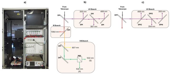
Figure 1.
(a) MULHACEN Raman lidar system operated at the Granada urban station. (b) Scheme of the MULHACEN receiving optics, divided in three different regions: Ultraviolet (UV), Infrared (IR), and Visible (VIS). Optical paths are represented by coloured arrows, dichroic mirrors (DM) by thin rectangles, and the polarising beam splitter (PBS) by a divided square. The different wavelength values correspond to the respective interference filters. (c) Updated optical configurations. Modified from [30].
The AGORA station also operates a SP within the framework of the AERONET [28]. The main instrument of AERONET is the Cimel sun photometer, which performs direct sun and sky radiance measurements at various wavelengths and provides AOD at 340, 380, 440, 670, 870, and 1020 nm. Particularly, we used Level 2.0 version 3 data [32]. In addition, the AGORA station is equipped with a GRAW DFM–09 RS, a lightweight radiosonde that provides measurements of temperature (resolution 0.01 ºC, accuracy 0.2 ºC), pressure, (resolution 0.1 hPa, accuracy 0.3 hPa), relative humidity (RH, resolution 1%, accuracy better than 4%) [10].
3. Methodology
3.1. Water Vapour Mixing Ratio Retrieval from Raman Lidar Measurements
The water vapour Raman lidar technique is based on the ratio of Raman scattering intensities from water vapour and the molecular reference [16]. The Raman lidar equation for the molecular reference and water vapour signals can be written as follows:
where index i indicates the molecular reference or water vapour molecule; is the backscattered signal from range z at the Raman-shifted wavelength ; is the emitted laser power at the wavelength ; is the range-independent system calibration constant, which accounts for the system optical efficiency, the telescope receiver area, the photomultiplier tube (PMT) spectral efficiency, and the laser output energy. is the overlap function; is the temperature-dependent function of the Raman scattering [15,33]; is the number density; is the cross section at the Raman-shifted wavelength; and the exponential term represents the atmospheric transmission function () due to the total extinction coefficient at wavelengths and .
The ratio is proportional to the water vapour mixing ratio (r), which is defined as the mass of water vapour divided by the mass of dry air in a sample of the atmosphere [34] allowing the Raman lidar technique to provide a direct measurement of the atmospheric water vapour [16]. Assuming identical overlap functions and range-independent Raman Backscatter cross sections for the molecular reference and :
and thus,
where the term represents the backscattered signal ratio, is the ratio of the temperature-dependent functions for the Raman molecular reference and channels, K is the calibration constant. The exponential term represents the differential atmospheric transmission that occurs at the two Raman-shifted wavelengths, and , where the total extinction coefficient at range z and wavelength is the sum of the molecular extinction and aerosol extinction coefficients. The equation can be rewritten as follows:
The assumption of identical overlap functions for the molecular reference and might not be true in real applications and differences between both overlap functions are found in the near range [33]. The temperature dependence of pure rotational and vibrational–rotational Raman was presented by [15], who assessed the required filter passbands for water vapour measurements with minimal temperature sensitivity using Nd:YAG lasers. According to this assessment the filters used in the MULHACEN Raman lidar for water vapour (centred at ∼408 nm, Full Width at Half Maximum (FWHM) = 1 nm) and molecular reference (centred at ∼387 nm, FWHM = 2.7 nm, or centred at ∼354 nm, FWHM = 0.8 nm) select the Raman Stokes spectrum (∼387 nm) or Raman Anti–Stokes spectrum (∼354 nm), resulting in essentially temperature independent measurements of the Raman signals, and making it reasonable to approximate the ratio to 1 [15]. Once the differential atmospheric transmission is accounted for, the calibration constant (K) is determined by comparing lidar profiles with simultaneous and co–located radiosonde measurements of water vapour using the iterative least squares method [10].
3.2. Differential Atmospheric Transmission Assessments
The differential atmospheric transmission in the retrieval of the water vapour mixing ratio arises from the difference in atmospheric transmission at the two wavelengths, and . This difference is mainly due to the dependence of Rayleigh scattering by air molecules [16], with an additional contribution from the wavelength-dependent Mie scattering by aerosols. The molecular extinction coefficient can be calculated for Rayleigh scattering [35] using temperature and pressure profiles. In this study, these profiles were obtained from ECMWF model data for the location of Granada [36], available from the ACTRIS Data Centre: https://hdl.handle.net/21.12132/1.16d392060df54287, accessed on 13 October 2025. The aerosol extinction coefficient can be retrieved directly using the Raman inversion method [37], or indirectly from aerosol backscatter coefficients retrieved with the Klett inversion method [38,39], multiplied by an assumed lidar ratio. In this study, the aerosol extinction coefficient was obtained by multiplying the aerosol backscatter coefficient () at 355 nm by a height-independent lidar ratio of 50 sr. This lidar ratio value has been used in previous studies at our station [40,41]. To estimate the aerosol backscatter coefficients at the Raman wavelengths (354, 387, and 408 nm), the spectral dependence of the backscatter was considered using the Ångström law [42], with the Ångström exponent (AE) derived from at 355 and 532 nm, both of which are emitted by MULHACEN. These profiles are also available from the EARLINET network (https://data.earlinet.org/earlinet/, accessed on 13 October 2025).
Ideally, the impact of aerosols on water vapour mixing ratio retrievals could be addressed if measurements at 355 nm were available. However, possible misalignments between backscatter and Raman measurements make this impossible. Additionally, the differences in the incomplete overlap region for the backscatter signal at 355 nm led us to look for an alternative to minimise this effect. Under such circumstances, many previous studies [10,14,18,19,20,21,22] have neglected , particularly in the analyses of very large databases due to computational effort. But the calculation of is a crucial step in the accurate retrieval of water vapour from Raman lidar measurements, as uncalculated systematic uncertainties on the order of 5–15% can introduce long-term biases in water vapour measurements. In addition, depending on the aerosol load, up to an additional 5% may be required in this term [16,17]. The impact of neglecting this term becomes more significant for Raman lidars that retrieve water vapour using VR water vapour and RR channels, due to the larger spectral separation between the molecular reference and water vapour Raman wavelengths. In contrast, once properly accounted for, these uncertainties can be treated as random. Since random uncertainties have an expected value of zero by definition, their impact can be reduced by increasing the number of observations [27].
To address this challenge, the present study proposes an approximation for the calculation aiming to overcome the considerable computational effort required for the automatic and operational retrieval of aerosol extinction coefficients. This approach is based on AOD values obtained from a sun photometer and the modelling of the vertical distribution of aerosol extinction using an exponential decay function of aerosol extinction with altitude [43]. Accordingly, the vertical profile of aerosol extinction coefficient is expressed as follows:
where is the surface extinction and is the scale height. In this study, is taken as the ABL height (), which was determined for Granada urban station by [44].
When using AOD() for the total aerosol load, Equation (5) is given as follows:
AOD values at 354, 387, and 408 nm were derived from the AOD at 380 nm using the AE between 340 and 440 nm from sun photometer measurements.
4. Results and Discussion
4.1. Sensitivity of the Differential Atmospheric Transmission with Wavelength
The sensitivity of the differential atmospheric transmission to wavelength is shown in Figure 2. The upper panels correspond to the first optical configuration used to retrieve the water vapour mixing ratio with the MULHACEN Raman lidar system, which employed the VR nitrogen channel at ∼387 nm, while the lower panels present results for the second configuration, which used the RR signal at ∼354 nm for the molecular reference. In both configurations, the water vapour Raman signal was measured at ∼408 nm. Particularly, Figure 2 presents the mean and standard deviation (SD) profiles of (panels a, d), (panels b, e) and (panels c, f) for the period 2010–2016, during which a total of 300 lidar aerosol inversions were performed. Molecular extinction profiles were calculated using temperature and pressure data from the ECMWF model for the Granada urban station. Aerosol extinction profiles were derived by multiplying the aerosol backscatter coefficients measured by the MULHACEN lidar system by a lidar ratio of 50 sr. Panel (c) includes a zoomed inset to better illustrate the profiles of the first configuration, allowing for a clearer comparison with the second (panel f). A statistical analysis of the mean calculation of for different layers is also presented in Table 1.
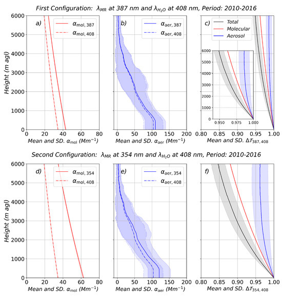
Figure 2.
(a) Molecular extinction coefficient at (solid line) and (dash–dot line). (b) Aerosol extinction coefficient at and from the MULHACEN Raman lidar. (c) Differential atmospheric transmission for total (black), molecular (red), and aerosol (blue) contributions. All profiles represent the mean and SD (shaded areas) over the 2010–2016 period at the Granada urban station for the first optical configuration. Standard deviation intervals for molecular extinction coefficients and molecular contribution to differential atmospheric transmission are small but present. (d–f) The lower panels display the same information for second optical configurations.

Table 1.
Statistical analysis of the differential atmospheric transmission at different layers, using the first and second optical configurations of the MULHACEN system for water vapour mixing ratio retrieval. Values are presented as mean bias ± standard deviation. The percentage by which the term deviates from unity is also provided. The aerosol profile database was acquired by the MULHACEN Raman lidar over the period 2010–2016.
Results from Figure 2 show an increase with height of and of its standard deviation (panels c and f, shaded areas), which is explained by the increased scattering due to molecules and aerosols as the path length increase. For the first configuration (VR nitrogen at ∼387 nm), neglecting the total differential transmission term may introduce systematic uncertainties of approximately 3.4% at 3 km, where most of the atmospheric water vapour is typically concentrated. The uncertainty may increase to 5.1% at 6 km (black curve in Figure 2c). On the other hand, for the second configuration that uses RR signal at ∼354 nm (Figure 2, lower panels) larger values in are observed. These reach approximately 10% at 3 km and 15% at 6 km (black curve in Figure 2f) (Table 1). These higher values of are explained by the larger spectral difference between the RR signal (∼354 nm) and water vapour (∼408 nm) signal. It should be noted that, the molecular component influence becomes more considerable than the aerosol one due to the of molecular scattering as opposed to the roughly dependence of aerosol scattering. Specifically, reaches about 7.0% at 3 km and 12% at 6 km (red curve in Figure 2f). Similarly, the aerosol contribution (blue curve in Figure 2f) presents larger values than in the previous configuration, with values of approximately 3.3% at 3 km and 4.0% at 6 km (Table 1).
Figure 2 and Table 1 clearly show that not including the calculation of in Equation (3) would introduce a significant systematic effect in water vapour mixing ratio retrievals. According to the recommendations of the Joint Committee for Guides in Metrology in their Guide to the Expression of Uncertainty in Measurement [JCFG/GUM] [27], “it is assumed that the result of a measurement has been corrected for all recognised significant systematic effects and that every effort has been made to identify such effects.” This principle is the driving force behind the requirement to include these calculations in the proper evaluation of the water vapour mixing ratio and has been performed in previous studies which used the VR nitrogen Raman signal at ∼387 nm [16,17].
We demonstrate that these effects are even more significant when using RR signal at ∼354 nm for the molecular reference. Ideally, should be calculated using correlative temperature and pressure profiles from radiosonde measurements. If such data are unavailable, calculations can be made using profiles from numerical weather models, which, despite possible differences, may still be used to convert systematic uncertainties into random uncertainties. For aerosols, the ideal correction uses correlative lidar measurements of . However, when these are not available, we propose an approach based solely on correlative AOD measurements, which similarly may translate systematic uncertainties into random uncertainties.
4.2. Sensitivity of Differential Atmospheric Transmission on Aerosol Loading
The dependence of the differential atmospheric transmission on aerosol loading is evaluated using different ranges of AOD values, as illustrated in Figure 3, differentiating between the VR (panel a) and RR (panel b) molecular reference configurations. The AOD values were obtained by integrating of the aerosol at 355 nm from MULHACEN lidar inversions. Data correspond to the 2010–2016 measurement period at the Granada EARLINET/ACTRIS station, where the mean and SD of value were of 0.28 ± 0.1. The effect in caused by molecular scattering alone (red curve) is also included for comparison. The aerosol load conditions (blue curves) considered in the calculation of range from very low AOD values to relatively high aerosol load conditions (solid blue curve). Specifically, low aerosol load corresponds to AOD values below the mean minus one SD (i.e., less than 0.18), medium aerosol load includes AOD values between the mean minus and plus one SD (from 0.18 to less than 0.38, dash–dot blue curve), and high aerosol load refers to AOD values equal to or greater than the mean plus one SD (0.38 or higher). In addition, Table 2 presents a statistical analysis of the mean calculation of , evaluated across different layers and aerosol loading conditions.
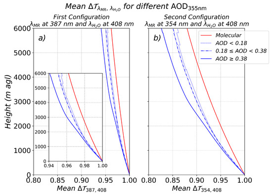
Figure 3.
(a) Differential Atmospheric Transmission curves for different aerosol loadings, ranging from a purely molecular (Rayleigh) atmosphere (red curve) to high aerosol load conditions (AOD at 355 nm ≥ 0.38, solid blue curve). These calculations correspond to the first optical configuration used for retrieving water vapour mixing ratio with the MULHACEN Raman lidar. All profiles represent the mean over the 2010–2016 period at the Granada urban station. (b) Same as panel (a), but for the second optical configuration of MULHACEN.
Table 2.
Statistical analysis of the differential atmospheric transmission at different layers and aerosol loading conditions, using the first and second optical configurations of the MULHACEN system for water vapour mixing ratio retrieval. Values are presented as mean bias ± standard deviation. The percentage by which the term deviates from unity is also provided. The aerosol profile database was acquired by the MULHACEN Raman lidar over the period 2010–2016.
Results from Figure 3 reveal that the influence of increases with aerosol loading, showing larger deviations from unity as AOD increases. Consequently, if is neglected, higher aerosol loads lead to greater systematic uncertainties in water vapour mixing ratio retrievals. For the first configuration (panel a), the results show that percentage differences in from unity reach values between 4.5% and 6% up to 6 km for low and high aerosol load conditions, respectively (Table 2). These values are consistent with those reported in previous studies [15,16], and illustrate that must be included in the calculation of mixing ratio in order to convert systematic uncertainties into random ones.
The most relevant result is that the effect of is clearly more significant for the second configuration, and this impact strongly depends on aerosol loading. In particular, under locally high aerosol load conditions (solid blue curve in Figure 3b), the total calculation reaches approximately 18% up to 6 km, compared to 12% when considering only the Rayleigh scattering calculation (Table 2). For medium and low aerosol load conditions (dash–dot and dotted blue curves in Figure 3b), the additional mean within the first 6 km required relative to the molecular case are approximately 2% and 3%, respectively (Table 2). Therefore, including in the calculation of water vapour mixing ratio is critical particularly for high aerosol loads that in the UGR station can reach values above 1.0 during extreme Saharan dust events [29].
4.3. Comparison of AOD from Sun Photometer and Raman Lidar Measurements
This study proposes an alternative approach to estimate the aerosol extinction coefficient profiles to overcome the considerable computational effort required for the operational retrieval when the lidar overlap function is significant. The approach is based on SP AOD values and assumes an exponential decay function of aerosol concentration with altitude (Equation (6), Section 3.2). To ensure the quality of the estimated aerosol profiles, SP AOD values were compared with those obtained by integrating aerosol extinction profiles retrieved from MULHACEN Raman lidar measurements. The comparison was carried out using simultaneous daytime AOD values, while for nighttime comparisons, the AOD values were estimated by interpolating between the last value in the previous afternoon and the first value in the next morning, as previously performed in other works in the literature [45].
This evaluation is illustrated in Figure 4 for the period 2010–2016, which presents the total dataset of 300 lidar measurements (panels a, d), daytime measurements (250 cases, panels b, e), and nighttime measurements (50 cases, panels c, f). The upper panels of Figure 4 show a direct inter-comparison of AOD values obtained by lidar versus those obtained by sun photometer, including the 1:1 reference line (dashed black) and the linear regression fit (solid red) with corresponding equations and uncertainties. The colour scales indicate magnitude of the residuals. The lower panels display histograms of the AOD differences (− ). The parameters of the linear fits, as well as other statistical parameters, are summarised in Table 3. The mean SP AOD values at 355 nm for the total, daytime and nighttime datasets were 0.25 ± 0.09, 0.26 ± 0.09, and 0.23 ± 0.07, respectively.
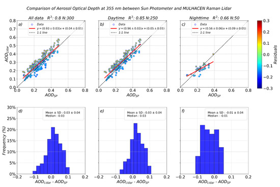
Figure 4.
Upper panels show scatter plots of lidar-derived AOD versus SP AOD at 355 nm for the period 2010–2016: (a) entire dataset, (b) daytime cases, and (c) nighttime cases. Red lines indicate the linear regression fits, dashed black lines represent the 1:1 line, and the colour scale corresponds to the residuals. Lower panels (d–f) display histograms of AOD differences (lidar − SP) for the same datasets: (d) total, (e) daytime, and (f) nighttime.
Table 3.
Linear fit parameters (slope, intercept, and ) between AOD values from MULHACEN Raman lidar and SP for the total, daytime, and nighttime datasets. The table also includes statistics on the differences between AOD values.
For the complete and daytime datasets, the linear regressions (Figure 4a,b) show good agreement between lidar and sun photometer ( of 0.80 and 0.85, respectively). In both cases, the slope of the linear fits (0.93 ± 0.03 and 0.96 ± 0.03) suggest an overestimation of lidar AOD values compared with reference sun photometer measurements (approximately 7%), which is supported by the bias and root mean square error (RMSE) values of 0.03 ± 0.04 and 0.05, respectively (Table 3). This overestimation may be related to the constant assumption of lidar ratio or to issues associated with the incomplete overlap region. Histograms (Figure 4d,e) display an approximately Gaussian shape centred near zero, although slightly skewed towards negative values, consistent with previous findings indicating a tendency for lidar to overestimate AOD [46,47,48]. Nevertheless, the fact that the histograms are centred close to zero plus the values of the residuals confirm that the majority of differences cluster near zero indicates no significant systematic uncertainties across the AOD range and further supports the robustness of the comparison.
The nighttime comparison (Figure 4c, Table 3) shows somewhat poorer agreement between lidar and sun photometer compared to the previous cases. The linear fit yields an of 0.66, which, although modest, remains statistically significant at the 95% confidence level. The linear regression indicates that for AOD values below 0.2, lidar values tend to be slightly higher than those from the SP, whereas for AOD values above 0.2, lidar values tend to be lower. This pattern is reflected by a small negative bias of −0.01 ± 0.04. The histogram of differences (Figure 4f) is centred at zero but does not show a clear Gaussian shape with a relatively high frequency of values in the extremes. This large dispersion may be attributed to increased uncertainties introduced by the interpolation approach used to estimate nighttime AOD, which could be minimised if actual nocturnal measurements were available, for example, through star [49,50] or moon photometry [51]. Nevertheless, the results demonstrate that estimating nighttime AOD by interpolating daytime sun photometer data provides a reasonable approximation for calculating , because the fundamental requirement for a satisfactory correction is that its mean value be zero [27]. If the random component increases through a given procedure, this is acceptable as long as the mean remains zero, and effective can be used to transform systematic uncertainties into random ones albeit with larger random uncertainties during the nighttime.
4.4. Validation of Differential Atmospheric Transmission Estimated from Sun Photometer Against Raman Lidar
The aerosol extinction coefficients profiles are estimated from AERONET sun photometer AOD values using an exponential decay function (Equation (6), Section 3.2). Based on these estimates, due to aerosols is calculated (Equations (3) and (4)). These simulated are then compared with reference profiles obtained from 300 aerosol extinction profiles retrieved by lidar inversion. Validation of the exponential decay approach is presented in Figure 5, including results for both the first (vibrational–rotational nitrogen at ∼387 nm) and second (pure–rotational signal at ∼354 nm for the molecular reference) optical configurations of the MULHACEN Raman lidar system. Additionally, statistical summaries of the comparisons are provided in Table 4.
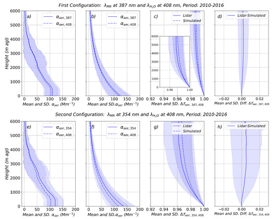
Figure 5.
(a) Aerosol extinction coefficient at (solid curve) and (dash–dot curve) as retrieved from the MULHACEN system. (b) Simulated aerosol extinction coefficient using an exponential decay function. (c) Differential atmospheric transmission due to aerosol contributions are shown for both lidar (solid curve) and simulations (dash–dot curve). (d) Differences between lidar and simulated aerosol differential transmission. All profiles represent the mean and SD (shaded areas) over the 2010–2016 period at the Granada urban station. Upper panels correspond to the first optical configurations of the MULHACEN system. (e–h) The lower panels show the same as the upper panels, but for the second optical configuration.
Table 4.
Statistical analysis of the aerosol differential atmospheric transmission at different layers, using the first and second optical configurations of the MULHACEN system for water vapour mixing ratio retrieval. Shown are the differences between lidar and simulated aerosol differential transmission. Values are presented as mean bias ± standard deviation. The percentage by which the term deviates from unity is also provided.
For both optical configurations, the simulated profiles—calculated using the exponential decay approach (Figure 5)—closely match the values obtained from the MULHACEN Raman lidar (panels c and g). Within the first 3 km, the mean aerosol contribution to is slightly lower in the simulations, with a 1.1% value compared to 1.2% from lidar inversions for the configuration employing VR nitrogen and water vapour channels (Figure 5c). For the configuration based on RR molecular reference and VR water vapour channels (Figure 5g), the mean value is 3.0% in the simulations and 3.3% in the lidar-derived data. At 6 km, simulated values are slightly lower than lidar-derived ones, with mean values of 1.2% (simulated) compared to 1.3% (lidar), and 3.5% versus 4.0% for the first and second optical configurations, respectively (panels c and g in Figure 5). The results shown in panels d and h of Figure 5 are particularly relevant, as the differences in the aerosol differential transmission calculation between the lidar and simulated values are nearly zero, with relative deviations of 0.10% and 0.40% within the 6 km for the first and second configurations, respectively (Table 4). These findings demonstrate a strong agreement between the simulations and the lidar measurements, with of 1.0, slope of 1.0 ± 0.0, and intercepts of 0.001 ± 0.00 and 0.002 ± 0.00 for molecular reference at ∼387 and ∼354 nm, respectively.
It is important to highlight that the residuals between the lidar-derived and simulated values of —using the exponential decay approach—exhibit a mean close to zero and a low standard deviation. This behaviour indicates that, when calculation of differential atmospheric transmission is included that the systematic uncertainties that are introduced when the term is not accounted for are be transformed into random uncertainties. This is particularly relevant for the retrieval of the water vapour mixing ratio, as random uncertainties can be statistically treated and propagated more robustly than systematic ones. Neglecting this term may lead to significant uncertainty in the water vapour retrieval [16,17]. Therefore, the proposed approach can minimise uncertainty and improve the accuracy of water vapour retrievals from Raman lidar measurements. The results demonstrate that this term can and should be calculated automatically and operationally using an exponential decay approach, offering a clear advantage over other studies in which it is often neglected [10,14,18,19,20,21,22].
Other studies, such as [17], have calculated the term by simulating the aerosol extinction profile using a step function. This approach assumes a well-mixed aerosol layer confined within the Atmospheric Boundary Layer (ABL), characterised by stability and an approximately homogeneous vertical distribution of aerosols. Under these conditions, it is reasonable to assume that the aerosol extinction coefficient remains constant with height within the ABL. Therefore, the total AOD is uniformly distributed throughout the ABL, and the aerosol extinction coefficient is considered constant within this layer and zero above it. We also applied this approach and found that the resulting calculations closely matched those obtained from lidar inversions, with of 1.0, a slope of 1.0 ± 0.0, and intercepts of −0.0001 ± 0.00 and −0.001 ± 0.00 for the molecular reference at ∼387 and ∼354 nm, respectively. The mean relative deviations between the simulated and lidar-derived calculations within the first 6 km were −0.03% and −0.10% for the first and second optical configurations of the MULHACEN system, respectively. However, the step function approach may be less accurate in the presence of decoupled aerosol layers above the ABL structures frequently observed at our station [29]. In such scenarios, the exponential decay method offers a more physically realistic representation of vertical aerosol distribution, reflecting natural processes such as the exponential decrease in atmospheric pressure with altitude. Despite their differences, both approaches are useful and provide a well-defined methodology for estimating the profile of aerosol extinction when no correlative measurements are available.
4.5. Evaluation of the Differential Atmospheric Transmission Calculation in Water Vapour Measurements
To evaluate the impact of the differential atmospheric transmission term on the retrieval of water vapour mixing ratio, Raman lidar water vapour profiles were calculated both considering and not considering the term (Equation (3)). It was assumed that the temperature dependence of the Raman backscatter cross sections is negligible, since the interference filters used to select the Raman scattering ensure a nearly temperature independent effect [15] (Section 3.1). After calculating (or not calculating) the differential transmission term, the calibration constant K was determined by comparison with radiosonde data, using the robust iterative least squares method proposed by [10]. The calculation (Equations (3) and (4)) was estimated using an exponential decay function (Equation (6)) based on SP AOD data.
Two different cases were analysed to investigate the effect of the differential atmospheric transmission term on Raman lidar water vapour measurements (Figure 6). Case I, on 11 July 2016 at 20:50 UTC (Figure 6, upper panels), corresponds to the period when the MULHACEN Raman lidar used the first optical configuration to retrieve the water vapour mixing ratio (VR nitrogen at ∼387 nm and VR water vapour at ∼408 nm). Case II, on 24 August 2017 at 19:36 UTC (Figure 6, lower panels), represents a study case where water vapour was retrieved using RR molecular reference at ∼354 nm and water vapour at ∼408 nm (second configuration). The Raman lidar water vapour mixing ratio profiles calculated including the , using the exponential decay approach are represented by a solid blue curve; and lidar profiles without are indicated by a dotted blue curve. Panels (b) and (e) in Figure 6 display the differences between the two water vapour mixing ratio profiles for Cases I and II, respectively, while the panels (c) and (f) show the relative differences.
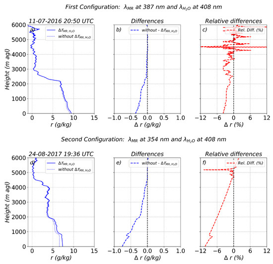
Figure 6.
(a) Water vapour mixing ratio profiles retrieved from Raman lidar on 11 July 2016 at 20:50 UTC, with (blue solid line) and without (blue dotted line) differential transmission calculation. (b) Differences between profiles without and with differential transmission calculation. (c) Relative differences, calculated with respect to the profiles with differential transmission calculation. The upper panels correspond to the first optical configuration of the MULHACEN system. (d–f) The lower panels show the same as the upper panels, but for the second optical configuration on 24 August 2017 at 19:36 UTC.
Cases I and II correspond to AOD at 355 nm of 0.31 (moderate aerosol load; see Section 4.2) and 0.38 (high aerosol load), respectively. These values result in total differential transmission at 6 km of 4.5% and 12.4%. In both cases, significant differences are observed between the water vapour mixing ratio profiles retrieved with and without calculating the differential transmission term (Figure 6). The maximum relative differences reach approximately −4% in Case I and −11% in Case II (panel c, f). Overall, the profiles excluding the calculation exhibit a systematic underestimation of water vapour compared to the ones including the calculation, with mean relative differences (using the fully calculated profiles as reference) in −2.3% and −4.0% within the first 6 km (Table 5). The most significant discrepancies are observed in the lower troposphere (below 3 km), where water vapour concentrations are typically highest and there is often strong aerosol concentrations. In this region, mean relative differences of −2.5% and −7.0% are found for Cases I and II, respectively. However, important differences are also present at higher altitudes, where, despite lower absolute humidity, the cumulative effect of differential transmission remains relevant (Table 5).
Table 5.
Differences between water vapour mixing ratio profiles retrieved without and with the calculation (r (g/kg)), evaluated across different layers. Values are presented as mean bias ± standard deviation within each layer. Precipitable water vapour are also included.
Furthermore, the impact of the molecular reference channel wavelength selection is clearly evident. In Case II (Figure 6, lower panels), where the spectral separation between the molecular reference and water vapour channels is larger, more pronounced differences are observed compared to Case I (Figure 6, upper panels). For instance, below 4 km, relative differences reach −6.0% in Case II compared to −2.6% in Case I, emphasising the greater need to account for the differential transmission when the spectral gap increases. Regarding the precipitable water vapour (W) retrieved from lidar, in Case I it is 18.90 ± 0.19 mm with the differential transmission, and 18.42 ± 0.20 mm without it. This corresponds to relative underestimations of 0.7% (with ) and 3.3% (without it) compared to the Global Navigation Satellite System (GNSS) value (19.04 ± 0.33 mm), illustrating that the including improves the agreement. In Case II, omitting the calculation of results in a 6% underestimation, while including it reduces the relative differences to only 0.2% (Table 5, GNSS W = 21.20 ± 0.12 mm). These results are consistent with the mean values reported in Table 1 and Table 2, and highlight the importance of including the differential transmission calculation to prevent systematic uncertainties in both vertical profiles and integrated water vapour estimates. Finally, it is important to note that neglecting this calculation introduces uncertainty in the determination of the calibration constant, as it would be derived from a signal affected by a bias. Consequently, this leads to a systematic uncertainty in the water vapour when using a specific calibration constant for subsequent retrievals. In contrast, our results demonstrate that the proposed approach enables the transformation of this systematic uncertainty into a random one, which can then be statistically treated, ultimately improving the reliability of the final product.
5. Summary and Conclusions
Accurate retrieval of the water vapour mixing ratio (r) from Raman lidar measurements requires precise calculation of the differential atmospheric transmission, , which accounts for the differences in molecular and aerosol extinction between the molecular reference and water vapour Raman-shifted wavelengths. Although this calculation is essential, since neglecting it often leads to significant systematic uncertainties in the retrieval of the water vapour mixing ratio—it has often been neglected in recent studies, potentially introducing long-term biases that compromise climate trend analyses and model validation. These uncertainties become more significant in systems with large spectral separation between Raman channels, such as those using a pure rotational (RR) filter to detect the molecular reference signal at ∼354 nm and a vibrational–rotational (VR) filter at ∼408 nm for water vapour. This is due to the wavelength dependence of molecules and Mie scattering.
This study presents a sensitivity analysis of of with respect to wavelength and aerosol loading, using lidar inversions and an operationally feasible approach based on sun photometer (SP) Aerosol Optical Depth (AOD) measurements, where aerosol extinction is modelled using an exponential decay function with altitude. Although this methodology cannot replace more robust retrievals based on the 355 nm backscatter signal, it effectively mitigates the limitations arising from misalignments between the backscatter and Raman channels, from incomplete-overlap effects, and even enables an approximate correction of aerosol effects for lidar systems lacking dedicated aerosol channels. The differential transmission term is determined for two optical configurations of the MULHACEN Raman lidar. The first configuration uses VR nitrogen at ∼387 nm and water vapour at ∼408 nm, while the second uses RR at 354 nm for the molecular reference and VR water vapour at ∼408 nm. A comprehensive statistical analysis of over 300 lidar inversions from the period 2010–2016 at the Granada urban station demonstrates that neglecting can lead to significant uncertainties, particularly under high aerosol loading, where values of up to 18% were observed. Up to 3 km–where most atmospheric water vapour resides–uncertainties in the retrieved water vapour mixing ratio can reach 4.0% and 12% for the first and second configurations, respectively. These uncertainties further increase to 6% and 18% up to 6 km. Based on measurements at the Granada station, including aerosols in the calculations can increase the magnitude of the differential transmission by as much as 6%.
Comparisons between lidar and SP AOD show strong agreement, with a slope of 0.93 ± 0.03, an intercept of 0.04 ± 0.01, and a determination coefficient of 0.80. This validates the use of SP AOD as a reliable estimate of the vertical aerosol extinction. The proposed AOD-based approach using exponential decay functions yields values that closely match those derived from lidar inversions. Relative deviations between simulated and lidar-derived calculations are close to zero, with relative deviations of 0.10% (0.40%) for ∼387 nm (∼354 nm) configurations. Importantly, residuals between lidar and simulated calculations are centred near zero with low standard deviation, indicating that including the calculation of can convert systematic uncertainties into random uncertainties. This is particularly valuable for water vapour retrievals, as random uncertainties can be statistically treated and propagated more robustly than systematic uncertainties and can be reduced by increasing the number of measurements. Neglecting may therefore introduce important uncertainty in water vapour mixing ratio retrievals.
For two different case studies corresponding to the two optical configurations of the MULHACEN Raman lidar system, calibration constants (K) for water vapour retrieval were determined with and without including the calculation. In Case I, neglecting the calculation resulted in relative underestimations of 3.3% in water vapour content relative to the GNSS value. When the calculation was included, this underestimation was reduced to 0.7%. In Case II, the underestimation was more pronounced, reaching 6% in water vapour content. Including the calculation reduced these differences to 0.2%, which is more critical if compared with the first configuration.
The proposed methodology enables the operational calculation of Raman lidar water vapour profiles using sun photometer data, making it suitable for long-term monitoring, climate research, and continental-scale water vapour characterisation. It is especially relevant for networks like EARLINET/ACTRIS, whose initial focus has been on aerosol studies but which can integrate water vapour as an operational product. Implementing these differential transmission calculations could improve the reliability and consistency of water vapour measurements, promoting their integration into regional and global climate assessments. Moreover, this approach reduces the dependency on the considerable effort required for lidar inversions to obtain aerosol extinction profiles, simplifying data processing and enhancing automation potential. By minimising systematic biases associated with differential atmospheric transmission, more accurate trend detection and model validation can be performed. Nevertheless, the exact equation for the approximation of must be fitted for each station because it ultimately depends on planetary boundary layer height and typical aerosol regime of each station.
Author Contributions
Conceptualisation, A.D.-Z., F.N.-G. and D.P.-R.; methodology, A.D.-Z., F.N.-G., D.P.-R., D.N.W. and V.M.N.-H.; formal analysis, A.D.-Z., V.M.N.-H., F.N.-G., D.P.-R., D.N.W., O.R.-N., L.A.-A. and J.M.-R.; investigation, A.D.-Z., V.M.N.-H., F.N.-G., D.P.-R., D.N.W., O.R.-N., L.A.-A. and J.M.-R.; resources, F.N.-G. and D.P.-R.; data curation, A.D.-Z. and V.M.N.-H.; writing—original draft preparation, A.D.-Z.; writing—review and editing, F.N.-G., D.P.-R., D.N.W., V.M.N.-H., O.R.-N. and J.M.-R.; supervision, F.N.-G., D.P.-R. and D.N.W.; project administration, F.N.-G. and D.P.-R.; funding acquisition, F.N.-G. and D.P.-R. All authors have read and agreed to the published version of the manuscript.
Funding
This research was funded by Grant PID2021-128008OB-I00 funded by MICIU/AEI/10.13039/501100011033 by ERDF/EU European Union.
Data Availability Statement
Temperature and pressure profiles for Granada were obtained from ECMWF model data, available from the ACTRIS Data Centre: https://hdl.handle.net/21.12132/1.16d392060df54287 (accessed on 13 October 2025). Lidar measurements are available from the EARLINET/ACTRIS network: https://data.earlinet.org/earlinet/ (accessed on 13 October 2025). Aerosol Optical Depth can be obtained from the AERONET network: https://aeronet.gsfc.nasa.gov/ (accessed on 13 October 2025). Additional data are available upon request from Francisco Navas-Guzmán (fguzman@ugr.es).
Acknowledgments
This work was supported mainly by the Spanish national projects CNS2023-145435, PID2023-151817OA-I00 and by the Horizon Europe programme under the Marie Skłodowska-Curie Staff Exchange Actions with the project GRASP-SYNERGY (grant agreement no. 101131631). The work made use of the strategic networks RED2022-134824-E and RED2024-153821-E and infrastructure grants EQC2019-006192-P and EQC2019-006423-P founded by MCIN/AEI /10.13039/501100011033, ATMO-ACCESS grant agreement No 101008004, ACTRIS-IMP grant agreement No 871115, and Scientific Unit of Excellence: Earth System (UCE-PP2017-02). It is also partially funded by the project AEROMOST (ProExcel_00204) by the “Junta de Andalucía”. Francisco Navas-Guzmán received funding from the Ramón y Cajal programme (ref. RYC2019-027519- I) of the Spanish Ministry of Science and Innovation. Víctor Manuel Naval Hernández thanks the Spanish Ministry of Science, Innovation and Universities for the grant FPU 23/01327 (co-funded by the European Social Fund Plus). We acknowledge ACTRIS and Finnish Meteorological Institute for providing the dataset which is available for download from https://cloudnet.fmi.fi (accessed on 13 October 2025). We acknowledge ECMWF for providing IFS model data.
Conflicts of Interest
The authors declare no conflicts of interest.
Abbreviations
The following abbreviations are used in this manuscript:
| RS | Radiosonde |
| MR | Molecular Reference |
| VR | Vibrational–Rotational |
| EARLINET | European Aerosol Research Lidar Network |
| ACTRIS | Aerosol, Clouds, and Trace Gases Research Infrastructure |
| RR | Pure–Rotational |
| SNR | Signal–to–Noise Ratio |
| UGR | Granada urban station |
| AOD | Aerosol Optical Depth |
| AERONET | Aerosol Robotic Network |
| SP | Sun Photometer |
| AGORA | Global ObseRvatory of the Atmosphere |
| PMT | Photomultiplier tube |
| JCFG | Joint Committee for Guides in Metrology |
| GUM | Guide to the Expression of Uncertainty in Measurement |
| ABL | Atmospheric Boundary Layer |
| GNSS | Global Navigation Satellite System |
References
- Douville, H.; Raghavan, K.; Renwick, J.; Allan, R.; Arias, P.; Barlow, M.; Cerezo-Mota, R.; Cherchi, A.; Gan, T.; Gergis, J.; et al. Water Cycle Changes. In Climate Change 2021: The Physical Science Basis. Contribution of Working Group I to the Sixth Assessment Report of the Intergovernmental Panel on Climate Change; Masson-Delmotte, V., Zhai, P., Pirani, A., Connors, S., Péan, C., Berger, S., Caud, N., Chen, Y., Goldfarb, L., Gomis, M., Eds.; Cambridge University Press: Cambridge, UK; New York, NY, USA, 2021; Chapter 8; pp. 1055–1210. [Google Scholar] [CrossRef]
- Ferrare, R.; Ismail, S.; Browell, E.; Brackett, V.; Clayton, M.; Kooi, S.; Melfi, S.H.; Whiteman, D.; Schwemmer, G.; Evans, K.; et al. Comparison of aerosol optical properties and water vapor among ground and airborne lidars and Sun photometers during TARFOX. J. Geophys. Res. Atmos. 2000, 105, 9917–9933. [Google Scholar] [CrossRef]
- Niemeier, U.; Wallis, S.; Timmreck, C.; van Pham, T.; von Savigny, C. How the Hunga Tonga—Hunga Ha’apai water vapor cloud impacts its transport through the stratosphere: Dynamical and radiative effects. Geophys. Res. Lett. 2023, 50, e2023GL106482. [Google Scholar] [CrossRef]
- Haefele, A.; Hocke, K.; Kämpfer, N.; Keckhut, P.; Marchand, M.; Bekki, S.; Morel, B.; Egorova, T.; Rozanov, E. Diurnal changes in middle atmospheric H2O and O3: Observations in the Alpine region and climate models. JGR Atmos. 2008, 113, 60. [Google Scholar] [CrossRef]
- Reichardt, J.; Wandinger, U.; Klein, V.; Mattis, I.; Hilber, B.; Begbie, R. RAMSES: German meteorological service autonomous Raman Iidar for water vapor, temperature, aerosol, and cloud measurements. Appl. Opt. 2012, 51, 8111–8131. [Google Scholar] [CrossRef]
- Navas-Guzmán, F.; Martucci, G.; Coen, M.C.; Granados-Muñoz, M.J.; Hervo, M.; Sicard, M.; Haefele, A. Characterization of aerosol hygroscopicity using Raman lidar measurements at the EARLINET station of Payerne. Atmos. Chem. Phys. 2019, 19, 11651–11668. [Google Scholar] [CrossRef]
- Perez-Ramirez, D.; Whiteman, D.N.; Veselovskii, I.; Ferrare, R.; Titos, G.; Granados-Munoz, M.J.; Sanchez-Hernandez, G.; Navas-Guzman, F. Spatiotemporal changes in aerosol properties by hygroscopic growth and impacts on radiative forcing and heating rates during DISCOVER-AQ 2011. Atmos. Chem. Phys. 2021, 21, 12021–12048. [Google Scholar] [CrossRef]
- Whiteman, D.N.; Demoz, B.; Girolamo, P.D.; Comer, J.; Veselovskii, I.; Evans, K.; Wang, Z.; Sabatino, D.; Schwemmer, G.; Gentry, B.; et al. Raman lidar measurements during the International H2O Project. Part II: Case studies. J. Atmos. Ocean. Technol. 2006, 23, 170–183. [Google Scholar] [CrossRef]
- Whiteman, D.N.; Venable, D.; Landulfo, E. Comments on “Accuracy of Raman lidar water vapor calibration and its applicability to long-term measurements”. Appl. Opt. 2011, 50, 2170–2176. [Google Scholar] [CrossRef]
- Navas-Guzmán, F.; Fernández-Gálvez, J.; Granados-Muñoz, M.J.; Guerrero-Rascado, J.L.; Bravo-Aranda, J.A.; Alados-Arboledas, L. Tropospheric water vapour and relative humidity profiles from lidar and microwave radiometry. Atmos. Meas. Tech. 2014, 7, 1201–1211. [Google Scholar] [CrossRef]
- Sica, R.J.; Haefele, A. Retrieval of water vapor mixing ratio from a multiple channel Raman-scatter lidar using an optimal estimation method. Appl. Opt. 2016, 55, 763–777. [Google Scholar] [CrossRef]
- Kulla, B.S.; Ritter, C. Water vapor calibration: Using a raman lidar and radiosoundings to obtain highly resolvedwater vapor profiles. Remote Sens. 2019, 11, 616. [Google Scholar] [CrossRef]
- Turner, D.D.; Lesht, B.M.; Clough, S.A.; Liljegren, J.C.; Revercomb, H.E.; Tobin, D.C. Dry bias and variability in Vaisala RS80-H radiosondes: The ARM experience. J. Atmos. Ocean. Technol. 2003, 20, 117–132. [Google Scholar] [CrossRef]
- Guerrero-Rascado, J.L.; Ruiz, B.; Chourdakis, G.; Georgoussis, G.; Alados-Arboledas, L. One year of water vapour raman lidar measurements at the andalusian centre for environmental studies (CEAMA). Int. J. Remote Sens. 2008, 29, 5437–5453. [Google Scholar] [CrossRef]
- Whiteman, D.N. Examination of the traditional Raman lidar technique I Evaluating the temperature-dependent lidar equations. Appl. Opt. 2003, 42, 2571–2592. [Google Scholar] [CrossRef]
- Whiteman, D.N.; Melfi, S.H.; Ferrare, R.A. Raman lidar system for the measurement of water vapor and aerosols in the Earth’s atmosphere. Appl. Opt. 1992, 31, 3068–3082. [Google Scholar] [CrossRef]
- Whiteman, D.N. Examination of the traditional Raman lidar technique II Evaluating the ratios for water vapor and aerosols. Appl. Opt. 2003, 42, 2593–2608. [Google Scholar] [CrossRef]
- Brocard, E.; Philipona, R.; Haefele, A.; Romanens, G.; Mueller, A.; Ruffieux, D.; Simeonov, V.; Calpini, B. Raman lidar for meteorological observations, RALMO—Part 2: Validation of water vapor measurements. Atmos. Meas. Tech. 2013, 6, 1347–1358. [Google Scholar] [CrossRef]
- Foth, A.; Baars, H.; Girolamo, P.D.; Pospichal, B. Water vapour profiles from raman lidar automatically calibrated by microwave radiometer data during hope. Atmos. Chem. Phys. 2015, 15, 7753–7763. [Google Scholar] [CrossRef]
- Dai, G.; Althausen, D.; Hofer, J.; Engelmann, R.; Seifert, P.; Bühl, J.; Mamouri, R.E.; Wu, S.; Ansmann, A. Calibration of Raman lidar water vapor profiles by means of AERONET photometer observations and GDAS meteorological data. Atmos. Meas. Tech. 2018, 11, 2735–2748. [Google Scholar] [CrossRef]
- Martucci, G.; Voirin, J.; Simeonov, V.; Renaud, L.; Haefele, A. A novel automatic calibration system for water vapor Raman LIDAR. In Proceedings of the EPJ Web of Conferences, Crete, Greece, 17–29 August 2018; Volume 176. [Google Scholar] [CrossRef]
- Di Girolamo, P.; Rosa, B.D.; Flamant, C.; Summa, D.; Bousquet, O.; Chazette, P.; Totems, J.; Cacciani, M. Water vapor mixing ratio and temperature inter-comparison results in the framework of the Hydrological Cycle in the Mediterranean Experiment—Special Observation Period 1. Bull. Atmos. Sci. Technol. 2020, 1, 113–153. [Google Scholar] [CrossRef]
- Laj, P.; Lund Myhre, C.; Riffault, V.; Amiridis, V.; Fuchs, H.; Eleftheriadis, K.; Petäjä, T.; Salameh, T.; Kivekäs, N.; Juurola, E.; et al. Aerosol, Clouds and Trace Gases Research Infrastructure (ACTRIS): The European Research Infrastructure Supporting Atmospheric Science. Bull. Am. Meteorol. Soc. 2024, 105, E1098–E1136. [Google Scholar] [CrossRef]
- Veselovskii, I.; Whiteman, D.N.; Korenskiy, M.; Suvorina, A.; Perez-Ramirez, D. Use of rotational Raman measurements in multiwavelength aerosol lidar for evaluation of particle backscattering and extinction. Atmos. Meas. Tech. 2015, 8, 4111–4122. [Google Scholar] [CrossRef]
- Wu, D.; Wang, Z.; Wechsler, P.; Mahon, N.; Deng, M.; Glover, B.; Burkhart, M.; Kuestner, W.; Heesen, B. Airborne compact rotational Raman lidar for temperature measurement. Opt. Express 2016, 24, A1210–A1223. [Google Scholar] [CrossRef]
- Martucci, G.; Navas-Guzmán, F.; Renaud, L.; Romanens, G.; Gamage, S.M.; Hervo, M.; Jeannet, P.; Haefele, A. Validation of pure rotational Raman temperature data from the Raman Lidar for Meteorological Observations (RALMO) at Payerne. Atmos. Meas. Tech. 2021, 14, 1333–1353. [Google Scholar] [CrossRef]
- JCFG/GUM. Guide to the Expression of Uncertainty in Measurement—Part 6: Developing and Using Measurement Models; JCFG/GUM: Saint-Cloud, France, 2020. [Google Scholar]
- Holben, B.N.; Eck, T.F.; Slutsker, I.; Tanré, D.; Buis, J.P.; Setzer, A.; Vermote, E.; Reagan, J.A.; Kaufman, Y.J.; Nakajima, T.; et al. AERONET—A federated instrument network and data archive for aerosol characterization. Remote Sens. Environ. 1998, 66, 1–16. [Google Scholar] [CrossRef]
- Bazo, E.; Perez-Ramirez, D.; Valenzuela, A.; Martins, V.; Titos, G.; Cazorla, A.; Rejano, F.; Patrón, D.; Diaz-Zurita, A.; Garcia-Izquierdo, F.J.; et al. Phase matrix characterization of long-range transported Saharan dust using multiwavelength polarized polar imaging nephelometry. Atmos. Chem. Phys. 2024, 2024, 1–29. [Google Scholar] [CrossRef]
- Ortiz-Amezcua, P. Atmospheric Profiling Based on Aerosol and Doppler Lidar. Ph.D. Thesis, Universidad de Granada, Granada, Spain, 2019. [Google Scholar]
- Wandinger, U.; Apituley, A.; Blumenstock, T.; Bukowiecki, N.; Cammas, J.P.; Connolly, P.; de Maziere, M.; Dils, B.; Fiebig, M.; Freney, E.; et al. ACTRIS PPP D5.1: Documentation on Technical Concepts and Requirements for ACTRIS Observational Platforms. Ph.D. Thesis, Leibniz Institute for Tropospheric Research, Leipzig, Germany, 2018. [Google Scholar]
- Giles, D.M.; Sinyuk, A.; Sorokin, M.G.; Schafer, J.S.; Smirnov, A.; Slutsker, I.; Eck, T.F.; Holben, B.N.; Lewis, J.R.; Campbell, J.R.; et al. Advancements in the Aerosol Robotic Network (AERONET) Version 3 database—Automated near-real-time quality control algorithm with improved cloud screening for Sun photometer aerosol optical depth (AOD) measurements. Atmos. Meas. Tech. 2019, 12, 169–209. [Google Scholar] [CrossRef]
- Whiteman, D.N.; Demoz, B.; Girolamo, P.D.; Comer, J.; Veselovskii, I.; Evans, K.; Wang, Z.; Cadirola, M.; Rush, K.; Schwemmer, G.; et al. Raman lidar measurements during the International H2O Project. Part I: Instrumentation and analysis techniques. J. Atmos. Ocean. Technol. 2006, 23, 157–169. [Google Scholar] [CrossRef]
- Goldsmith, J.E. Turn-key Raman lidar for profiling atmospheric water vapor, clouds, and aerosols. Appl. Opt. 1998, 37, 4979–4990. [Google Scholar] [CrossRef]
- Bucholtz, A. Rayleigh-scattering calculations for the terrestrial atmosphere. Appl. Opt. 1995, 34, 2765–2773. [Google Scholar] [CrossRef]
- O’Connor, E. Model Data from Granada on 13 February 2025; ACTRIS Cloud Remote Sensing Data Centre Unit (CLU): Helsinki, Finland, 2025. [Google Scholar]
- Ansmann, A.; Riebesell, M.; Weitkamp, C. Measurement of atmospheric aerosol extinction profiles with a Raman lidar. Opt. Lett. 1990, 15, 746–748. [Google Scholar] [CrossRef]
- Klett, J.D. Stable analytical inversion solution for processing lidar returns. Appl. Opt. 1981, 20, 211–220. [Google Scholar] [CrossRef]
- Klett, J.D. Lidar inversion with variable backscatter/extinction ratios. Appl. Opt. 1985, 24, 1638–1643. [Google Scholar] [CrossRef]
- Müller, D.; Ansmann, A.; Mattis, I.; Tesche, M.; Wandinger, U.; Althausen, D.; Pisani, G. Aerosol-type-dependent lidar ratios observed with Raman lidar. JGR Atmos. 2007, 112, 411. [Google Scholar] [CrossRef]
- Guerrero-Rascado, J.L.; Olmo, F.J.; Avilés-Rodríguez, I.; Navas-Guzmán, F.; Pérez-Ramírez, D.; Lyamani, H.; Arboledas, L.A. Extreme saharan dust event over the southern iberian peninsula in september 2007: Active and passive remote sensing from surface and satellite. Atmos. Chem. Phys. 2009, 9, 8453–8469. [Google Scholar] [CrossRef]
- Ångström, A. On the Atmospheric Transmission of Sun Radiation and on Dust in the Air. Geogr. Ann. Ser. B 1929, 11, 156–166. [Google Scholar] [CrossRef]
- Gras, J.L. Southern Hemisphere tropospheric aerosol microphysics. J. Geophys. Res. Atmos. 1991, 96, 5345–5356. [Google Scholar] [CrossRef]
- Moreira, G.D.A.; Guerrero-Rascado, J.L.; Bravo-Aranda, J.A.; Foyo-Moreno, I.; Cazorla, A.; Alados, I.; Lyamani, H.; Landulfo, E.; Alados-Arboledas, L. Study of the planetary boundary layer height in an urban environment using a combination of microwave radiometer and ceilometer. Atmos. Res. 2020, 240, 104932. [Google Scholar] [CrossRef]
- Li, J.; Li, C.; Guo, J.; Li, J.; Tan, W.; Kang, L.; Chen, D.; Song, T.; Liu, L. Retrieval of aerosol profiles by Raman lidar with dynamic determination of the lidar equation reference height. Atmos. Environ. 2019, 199, 252–259. [Google Scholar] [CrossRef]
- Xie, C.B.; Zhou, J.; Wang, Z.F.; Sugimoto, N. Aerosol observation with Raman LIDAR in Beijing, China. J. Opt. Soc. Korea 2010, 14, 215–220. [Google Scholar] [CrossRef][Green Version]
- Sicard, M.; Rocadenbosch, F.; Reba, M.N.; ComerÓn, A.; Tomás, S.; García-Vízcaino, D.; Batet, O.; Barrios, R.; Kumar, D.; Baldasano, J.M. Seasonal variability of aerosol optical properties observed by means of a Raman lidar at an EARLINET site over Northeastern Spain. Atmos. Chem. Phys. 2011, 11, 175–190. [Google Scholar] [CrossRef]
- Mamouri, R.E.; Papayannis, A.; Amiridis, V.; Müller, D.; Kokkalis, P.; Rapsomanikis, S.; Karageorgos, E.T.; Tsaknakis, G.; Nenes, A.; Kazadzis, S.; et al. Multi-wavelength Raman lidar, sun photometric and aircraft measurements in combination with inversion models for the estimation of the aerosol optical and physico-chemical properties over Athens, Greece. Atmos. Meas. Tech. 2012, 5, 1793–1808. [Google Scholar] [CrossRef]
- Pérez-Ramírez, D.; Ruiz, B.; Aceituno, J.; Olmo, F.J.; Alados-Arboledas, L. Application of Sun/star photometry to derive the aerosol optical depth. Int. J. Remote Sens. 2008, 29, 5113–5132. [Google Scholar] [CrossRef]
- Pérez-Ramírez, D.; Lyamani, H.; Olmo, F.J.; Alados-Arboledas, L. Improvements in star photometry for aerosol characterizations. J. Aerosol. Sci. 2011, 42, 737–745. [Google Scholar] [CrossRef]
- Barreto, A.; Román, R.; Cuevas, E.; Pérez-Ramírez, D.; Berjón, A.J.; Kouremeti, N.; Kazadzis, S.; Gröbner, J.; Mazzola, M.; Toledano, C.; et al. Evaluation of night-time aerosols measurements and lunar irradiance models in the frame of the first multi-instrument nocturnal intercomparison campaign. Atmos. Environ. 2019, 202, 190–211. [Google Scholar] [CrossRef]


Disclaimer/Publisher’s Note: The statements, opinions and data contained in all publications are solely those of the individual author(s) and contributor(s) and not of MDPI and/or the editor(s). MDPI and/or the editor(s) disclaim responsibility for any injury to people or property resulting from any ideas, methods, instructions or products referred to in the content. |
© 2025 by the authors. Licensee MDPI, Basel, Switzerland. This article is an open access article distributed under the terms and conditions of the Creative Commons Attribution (CC BY) license (https://creativecommons.org/licenses/by/4.0/).