Article

Data Uncertainty of Flood Susceptibility Using Non-Flood Samples

1
School of Geography and Tourism, Anhui Normal University, Wuhu 241002, China
2
Engineering Technology Research Center of Resources Environment and GIS, Anhui Normal University, Wuhu 241002, China
3
State Key Laboratory of Earth Surface Processes and Resource Response in the Yangze-Huaihe River Basin, Anhui Normal University, Wuhu 241002, China
4
Hunan Institute of Water Resources and Hydropower Research, Changsha 410007, China
*
Author to whom correspondence should be addressed.
Remote Sens. 2025, 17(3), 375; https://doi.org/10.3390/rs17030375
Submission received: 21 November 2024 / Revised: 19 January 2025 / Accepted: 20 January 2025 / Published: 23 January 2025
(This article belongs to the Special Issue Remote Sensing in Hydrometeorology and Natural Hazards)

Abstract

:
Flood susceptibility provides scientific support for flood prevention planning and infrastructure development by identifying and assessing flood-prone areas. The uncertainty posed by non-flood sample datasets remains a key challenge in flood susceptibility mapping. Therefore, this study proposes a novel sampling method for non-flood points. A flood susceptibility model is constructed using a machine learning algorithm to examine the uncertainty in flood susceptibility due to non-flood point selection. The influencing factors of flood susceptibility are analyzed through interpretable models. Compared to non-flood datasets generated by random sampling with the buffer method, the non-flood dataset constructed using the spatial range identified by the frequency ratio model and sampling method of one-class support vector machine achieves higher accuracy. This significantly improves the simulation accuracy of the flood susceptibility model, with an accuracy increase of 24% in the ENSEMBLE model. (2) In constructing the flood susceptibility model using the optimal non-flood dataset, the ENSEMBLE learning algorithm demonstrates higher accuracy than other machine learning methods, with an AUC of 0.95. (3) The northern and southeastern regions of the Zijiang River Basin have extremely high flood susceptibility. Elevation and drainage density are identified as key factors causing high flood susceptibility in these areas, whereas the southwestern region exhibits low flood susceptibility due to higher elevation. (4) Elevation, slope, and drainage density are the three most important factors affecting flood susceptibility. Lower values of elevation and slope and higher drainage density correlate with higher flood susceptibility. This study offers a new approach to reducing uncertainty in flood susceptibility and provides technical support for flood prevention and disaster mitigation in the basin.

1. Introduction

Flooding is one of the most destructive natural disasters globally, causing significant losses to the global socioeconomic and ecological environment [1]. Due to global warming and human activities, the frequency and intensity of floods have markedly risen [2]. Natural factors affecting flood disasters mainly include hydrological conditions, environmental characteristics, and topographical conditions, such as prolonged precipitation, climate change, and land use changes. Furthermore, human factors, including inadequate water management projects, riverbank encroachment, and urbanization, are also critical in intensifying flood disasters [1]. Dongting Lake, China’s second-largest freshwater lake, serves as an essential regulatory lake in the Yangtze River Basin with substantial flood storage capacity, playing an indispensable role in the basin’s flood control system. However, in recent years, flooding has frequently occurred in the Dongting Lake Basin. In June 2024, partial dike breaches in Dongting Lake led to landslides, road collapses, and several emergencies in the Zijiang River Basin, resulting in substantial property damage. Flood susceptibility mapping serves as an essential tool for flood disaster defense, offering scientific support for regional flood control planning and playing a key role in risk management and emergency decision-making [3]. Therefore, it is urgent to conduct studies on flood susceptibility at the regional watershed scale to take measures that mitigate the impact of devastating floods [4].
With the rapid development of machine learning technology, numerous studies have applied it to flood susceptibility analysis and mapping in river basins, effectively improving the accuracy and reliability of flood risk assessment, thus providing more effective means to reduce flood disaster losses [5]. Numerous flood susceptibility models have been developed to create flood susceptibility maps based on local environmental characteristics. Flood susceptibility is analyzed using 1-D or 2-D hydrodynamic models based on information such as flood inundation extent, depth, and velocity [6,7]. However, physically based integrated hydrological and hydrodynamic models demand significant processing power and computation time, a substantial amount of hydrological and meteorological data for calibration, and parameter assessments describing the physical features of the watershed [8,9]. Furthermore, hydrodynamic models impose stringent demands on data conditions and computer hardware, complicating efficient large-scale simulations [9,10].
In recent years, more researchers have focused on combining GIS tools with statistical and machine learning methods to construct flood susceptibility models for flood susceptibility assessment [1,4]. Machine learning methods predict flood susceptibility by autonomously learning features of existing training samples, including methods such as Random Forest [11], support vector machine [12], decision tree [13], Gradient Boosted Tree [14], Artificial Neural Network [4], Convolutional Neural Network [15], Recurrent Neural Network [16], or Deep Learning Neural Network [17]. However, flood susceptibility modeling based on a single machine learning method has certain limitations, while hybrid ensemble machine learning algorithms can effectively reduce the uncertainties associated with single-model simulations [4]. Previous studies have used algorithms such as AUC-based weighted averaging, dagging, and stacking to construct high-precision flood susceptibility models for prediction, finding that the accuracy of ensemble models exceeds that of the original single models [4,18]. The high-accuracy predictions achieved by ensemble algorithms have encouraged the application of hybrid machine learning algorithms in constructing models for various types of natural disasters [19]. However, there is no general consensus on the optimal model for simulating various forms of natural disasters (e.g., landslides or flood susceptibility), highlighting the need to explore new methods for constructing and evaluating flood susceptibility maps and other forms of natural disaster simulations [20,21].
Data uncertainty is one of the most critical factors affecting the accuracy of flood susceptibility mapping, and further research is needed on how to improve model prediction accuracy by reducing data sample uncertainty. In current flood susceptibility models, efforts to reduce data uncertainty mainly focus on decreasing the number of influencing factors or optimizing their weight coefficients. Kanani-Sadat et al. [22] used a fuzzy-DEMATEL combined with ANP method to determine the weights of flood influencing factors, reducing the uncertainty in factor weights resulting from different expert decisions. Al-Aizari et al. [23] used a drop-off loop function to reduce prediction uncertainty caused by model overfitting due to an excessive number of influencing factors. Ekmekcioğlu et al. [24] reduced model output uncertainty caused by sample size by using flood and non-flood sample ratios of 1:1, 1:10, 1:25, 1:50, and 1:100. The selection of flood and non-flood sample datasets has a significant impact on the accuracy and rationality of susceptibility zoning [25]. Flood sample points can be extracted through field surveys, interpretation of remote sensing images during flood periods, and flood historical catalog data, with relatively high data quality. However, the selection of non-flood sample points only describes the extraction method [26,27], while the model inaccuracies introduced by non-flood points are often overlooked.
Some studies select non-flood points randomly in historically flood-free areas or areas with high flood protection standards [13,28], which accelerates model convergence and enhances classification accuracy [29]. However, these methods depend on historical data or expert opinion, failing to fully leverage the environmental characteristics of areas where floods have occurred to select non-flood sample points and overlooking the spatial distribution relationship between flooding and influencing factors. Moreover, the selection of negative samples is also present in other natural disaster susceptibility studies. For instance, Guo et al. used the buffer method to select non-landslide samples within local areas [30]. Ye et al. employed a one-class support vector machine (OC SVM) approach, incorporating regional environmental characteristics to generate more reasonable non-landslide samples, which, when used as negative samples, significantly improved the model’s predictive accuracy [31]. Therefore, accurately identifying flood and non-flood data sample sets is crucial for reducing data uncertainty in model research.
Hence, this study first proposes a method for extracting non-flood point samples that considers spatial range and sampling method. Then, it constructs a flood susceptibility model using machine learning algorithms and quantifies the uncertainty of non-flood samples on the accuracy of model predictions. Finally, SHAP interpretable models are used to provide a rationale for the prediction results of each model, identifying the most significant flood influencing factors. The results will support regional and local authorities and decision-makers in mitigating flood-related risks and facilitate the development of suitable mitigation strategies to prevent potential hazards.

2. Data and Research Framework
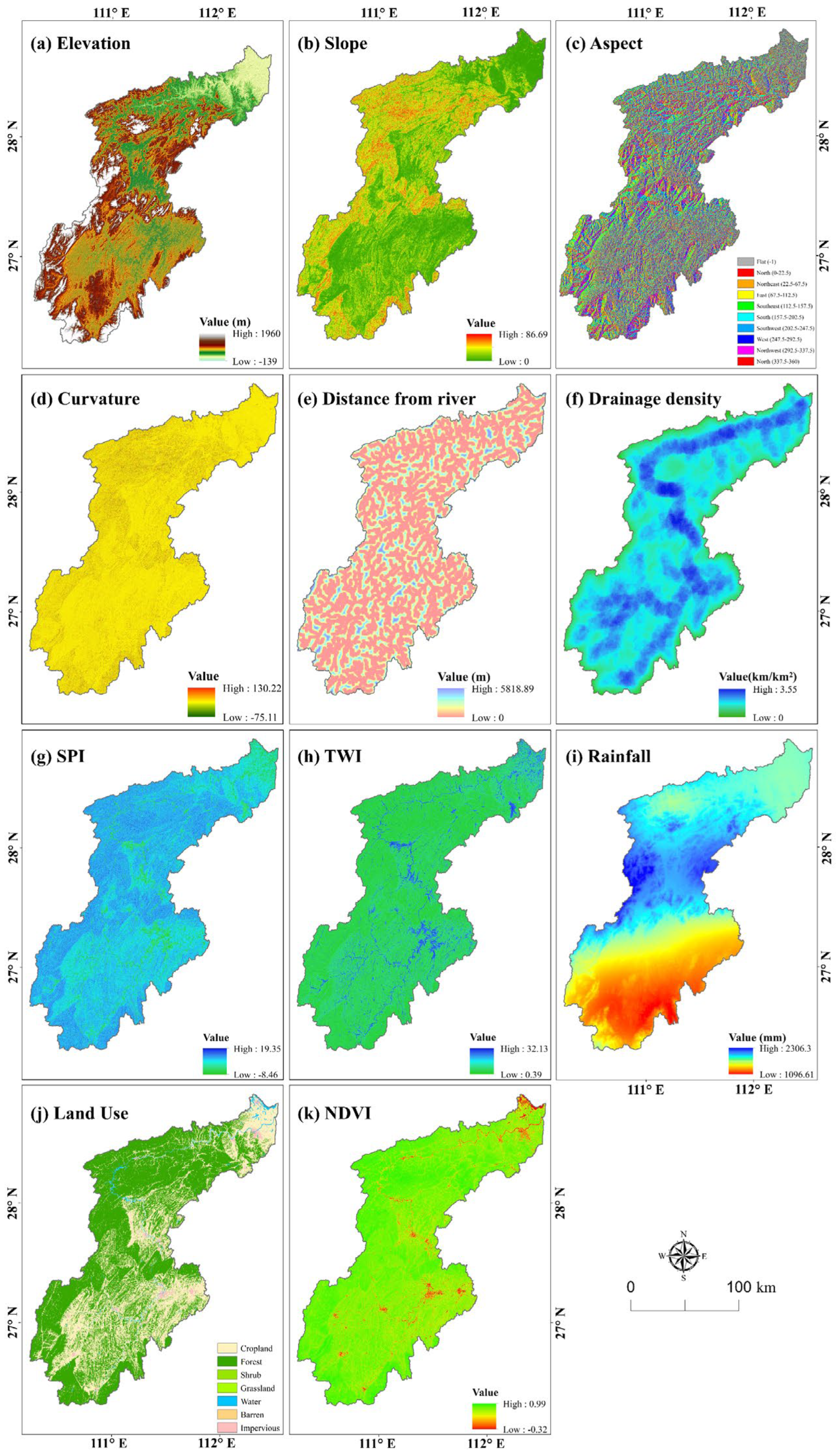
2.1. Data

The Zijiang River is an important tributary of Dongting Lake, with a basin that is long from north to south and narrow from east to west, featuring higher terrain in the southwest and lower terrain in the northeast. The main stream of the basin is 653 km long, with a basin area of 26,738 km2 within Hunan Province, accounting for 95.4% of the total basin area. The study area is a portion of the Zijiang River Basin within Hunan Province, as shown in Figure 1. The flood point data used in this study were obtained from the Hunan Provincial Institute of Water Resources.
Flood influencing factors are inputs for flood susceptibility models, and identifying the appropriate flood influencing factors for the study area is crucial for constructing a high-accuracy flood susceptibility model. Based on regional characteristics, available data, and commonly used flood susceptibility factors, the flood influencing factors were determined to include four topographic factors, four hydrological factors, and three supplementary factors. The topographic factors include elevation, slope, aspect, and curvature; the hydrological factors include river distance, drainage density, stream power index, and topographic wetness index; and the supplementary factors include rainfall, land use type, and normalized vegetation index. The detailed description and sources of the data are shown in Table 1.
The topographic and hydrological influencing factors of flood susceptibility are calculated using digital elevation model (DEM) data. The flood influencing factors were projected and standardized in spatial resolution to ensure they possess a common coordinate system and uniform spatial resolution (Figure 2).
(1) Elevation: During flood events, water tends to flow towards lower elevation areas within the basin, leading to a higher likelihood of flooding in these regions. In the Zijiang River Basin, the northeast is lower in elevation, while the southwest is higher (Figure 2a).
(2) Slope: As water moves from high slope areas to low slope regions, and due to the higher flow velocity at elevated locations, it is less likely to infiltrate underground, leading to accumulation in low slope areas. Consequently, areas with greater slope differences are more prone to flooding. The maximum slope in this region is approximately 86.69 (Figure 2b).
(3) Aspect: Aspect can impact the microclimate of an area, influencing parameters such as soil moisture and vegetation cover, and is a significant factor in flood susceptibility assessment. It is divided into nine categories, including eight directional aspects and one flat category (Figure 2c).
(4) Curvature: Curvature affects the concentration and dispersion of water flow [33] and is frequently employed in flood susceptibility modeling. It differentiates between concentrated and dispersed runoff areas [34], with negative values indicating regions of concentrated runoff [35], which are highly vulnerable to flash floods (Figure 2d).
(5) Distance to River: Rivers serve as vital channels for flood drainage, making areas near rivers particularly vulnerable to flooding, and vice versa [36]. The distance to the river varies from 0 to 5818.89 m (Figure 2e).
(6) Drainage Density: Drainage density quantitatively measures surface drainage. A higher drainage density indicates greater surface runoff, which increases the risk of flooding [37], thus serving as a crucial factor in assessing flood susceptibility (Figure 2f).
(7) SPI: The stream power index (SPI) is an indicator of water flow erosion and sediment movement in river channels [38]. Results from this index can identify areas where soil conservation practices mitigate the effects of concentrated surface runoff erosion (Figure 2g).
(8) TWI: The topographic wetness index (TWI) quantifies the potential accumulation of water flow and saturation of soil in specific areas [39]. Higher TWI values suggest increased flood risk in those regions (Figure 2h). TWI peaks at lower slopes with higher flow accumulation [40].
(9) Rainfall: The duration and amount of rainfall are crucial in flood events (Figure 2i). In areas experiencing extended rainfall, soil moisture absorption saturates, diminishing its ability to absorb further moisture and elevating flood risk [41]. The study uses average annual rainfall data as an indicator of flood susceptibility.
(10) Land Use: Different types of land use have varying abilities to facilitate the infiltration of surface water into the ground, significantly impacting this process. The greater the capacity for water infiltration, the lower the flood susceptibility; conversely, the lesser the capacity, the higher the susceptibility. In the Zijiang River Basin, land use is classified into seven categories: farmland, forest land, shrubland, grassland, water bodies, wasteland, and impervious surfaces, with agricultural and forest land comprising 96.4% and built-up areas accounting for 2.1% (Figure 2j).
(11) Vegetation Index: The vegetation index is a quantitative measure of plant vitality and abundance, as vegetation can mitigate flood risk by enhancing soil stability and absorbing moisture [42]. A higher vegetation index indicates greater vegetation cover in the area and enhanced capacity to alleviate flood risk (Figure 2k).

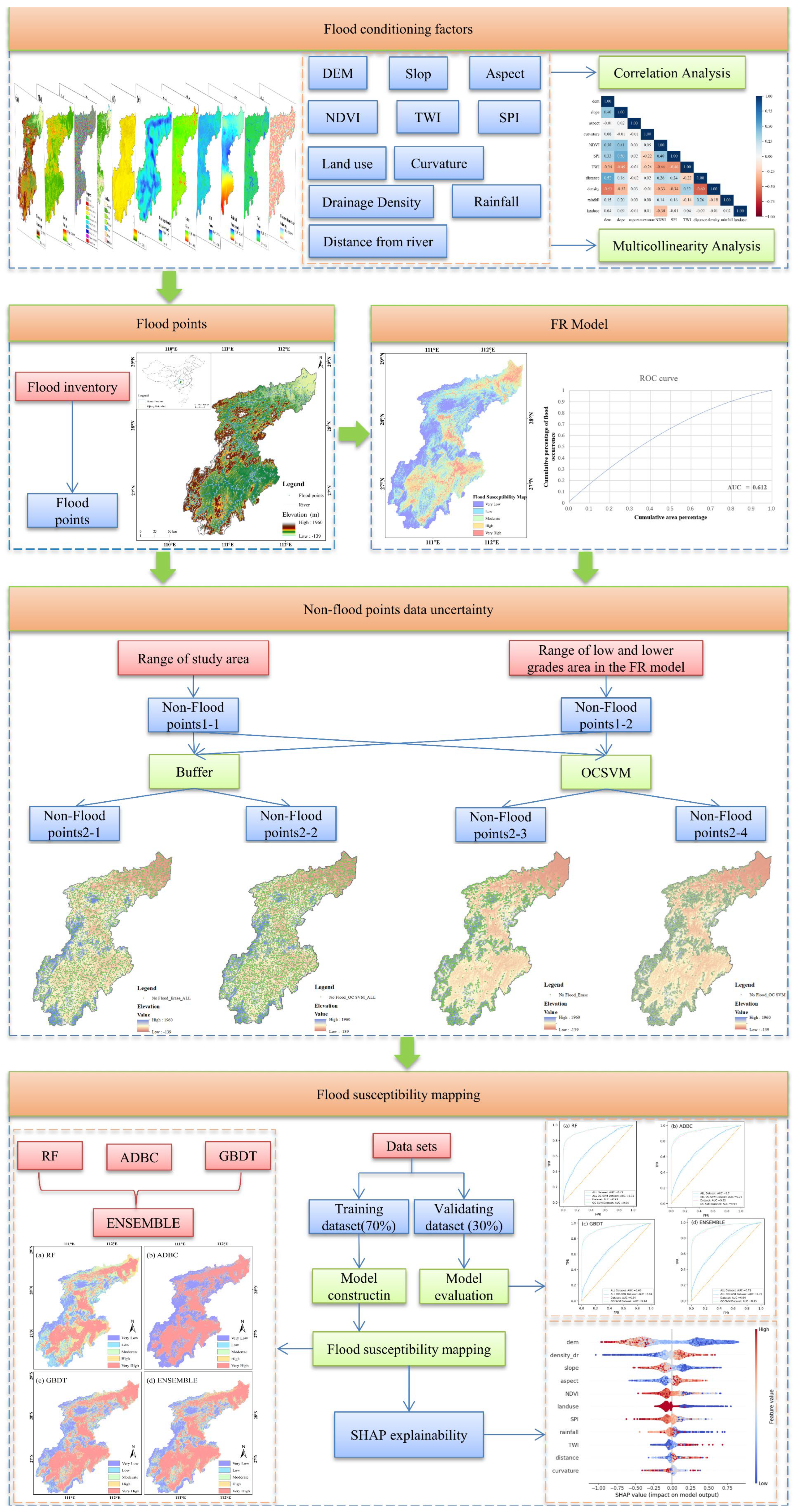
2.2. Research Framework

This study process is divided into five parts. The first step is data collection, including flood point location data and flood influencing factor data. The second step is redundancy analysis of influencing factors, including Pearson correlation coefficients and multicollinearity statistical indicators. The third step focuses on constructing non-flood point datasets by identifying medium and low flood susceptibility areas from the primary flood susceptibility results derived from statistical models, integrating the Buffer method and OC SVM method to generate four non-flood point datasets. The third step focuses on constructing non-flood point datasets by identifying medium and low flood susceptibility areas from the primary flood susceptibility results derived from statistical models, integrating the Buffer method and OC SVM method to generate four non-flood point datasets. The fourth step focuses on the uncertainty analysis of the flood susceptibility model. A flood susceptibility model is constructed using machine learning algorithms, and the accuracy of the model based on the four non-flood point datasets is utilized to quantify the uncertainty of the flood susceptibility model simulation. The fifth step is the interpretability analysis of the influencing factors, where the SHAP algorithm is introduced to enhance model interpretability, analyzing the relationship between model prediction results and flood influencing factors. This is shown in Figure 3.

3. Methods

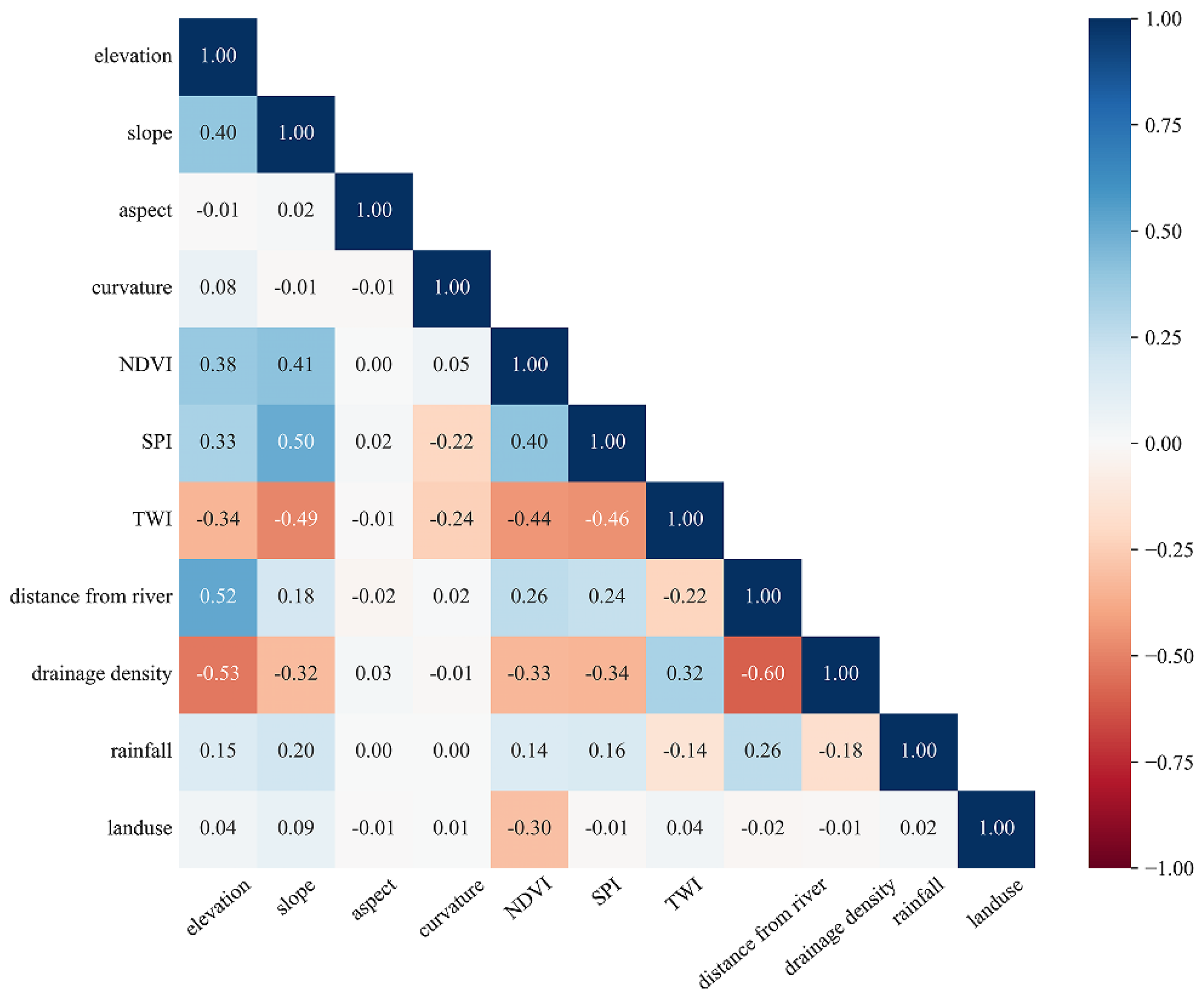
3.1. Multicollinearity Analysis

Three indicators were used to quantify the degree of correlation between flood impact factors: Pearson correlation coefficient [33], variance diffusion factor, and tolerance [43]. Spearman > 0.7 indicates high dependence [44]. Tolerance value (TOL) < 0.1 indicates that there is covariance between this independent variable and other independent variables, and there is strong multicollinearity when VIF ≥ 10.
T O L = 1 R j 2
V I F = 1 T O L
where R j 2 is the coefficient of the regression equation.

3.2. One-Class SVM

One-class SVM (OC SVM) is a machine learning algorithm for outlier detection [45]. Unlike algorithms that require two classes of sample data, one-class SVM is trained on single-class data and has the ability to quickly distinguish sample categories. The idea is to construct a hypersphere, map the identified single-class data onto the sphere, train the known data through a kernel function, and find the minimum radius R of the hypersphere. The sample category outside the hypersphere is used to detect outliers [46]. The method is used to identify potential flood points in the initial non-flood dataset, thus improving the quality of the non-flood dataset. It should be noted that flood conditioning factor data of the OC SVM model input need to be normalized before being processed, and the output data value is −1 to represent the non-flood point and 1 to represent the flood point.

3.3. Flood Susceptibility Modeling

3.3.1. FR

The frequency ratio method calculates the probability of floods occurring at different grading intervals for each impact factor and analyses the spatial relationship between the spatial distribution of floods and the grading of each impact factor. When the value is greater than 1, the relationship between the occurrence of floods and the impact factors is strong, while less than 1 indicates a low correlation [47].

3.3.2. RF

The Random Forest (RF) algorithm is a machine learning algorithm that classifies input datasets using multiple decision trees. It was originally developed based on the random subspace method [48]. Its basic idea is to train a decision tree on a random selection of a set of data features, and then to generate multiple decision trees. Finally, multiple decision trees are combined by majority voting or averaging to obtain the final result. In recent years, more and more researchers have paid attention to RF because it can achieve accurate classification results and efficient processing speed [49].

3.3.3. Adaptive Boosting

The AdaBoost (Adaptive Boosting) classifier algorithm was proposed by Freund and Schapire [50]. It essentially combines a set of decision trees, known as weak classifiers, into a stronger decision tree to improve the classification process, known in machine learning as lifting [51]. During the learning process, each weak classifier produces a Boolean expression (in this context, flooding or non-flooding) and executes a learned sequence. After each round, the samples are reweighted to find those that were misclassified in the previous round. When the specified threshold is reached, the sequence stops and the weighted set of weak classifiers produces a stronger classifier. Weak classifiers have lower weights when assigning incorrect classes, while good classifiers have higher weights [51]. This implements an adaptive learning sequence and optimizes the classification process.

3.3.4. Gradient Boosting

Gradient boosted decision trees (GBDTs) are a tree-based ensemble supervised machine learning technique introduced by Jerome H. Friedman to improve the performance of weak or basic classifiers [52]. Boosting involves the sequential construction of decision trees, where each successive tree attempts to minimize the error of the previous tree. Therefore, a key improvement is the use of a differentiable loss function for boosting in GBDT, which increases the elasticity of the algorithm to outliers [53]. The GBDT method differs from AdaBoost in that it generates a weak classifier in multiple iterations (typically using a CART regression tree), each of which is trained on the residuals from the last iteration of the classifier. In each iteration, the weak classifiers are weighted and summed to produce the final result.

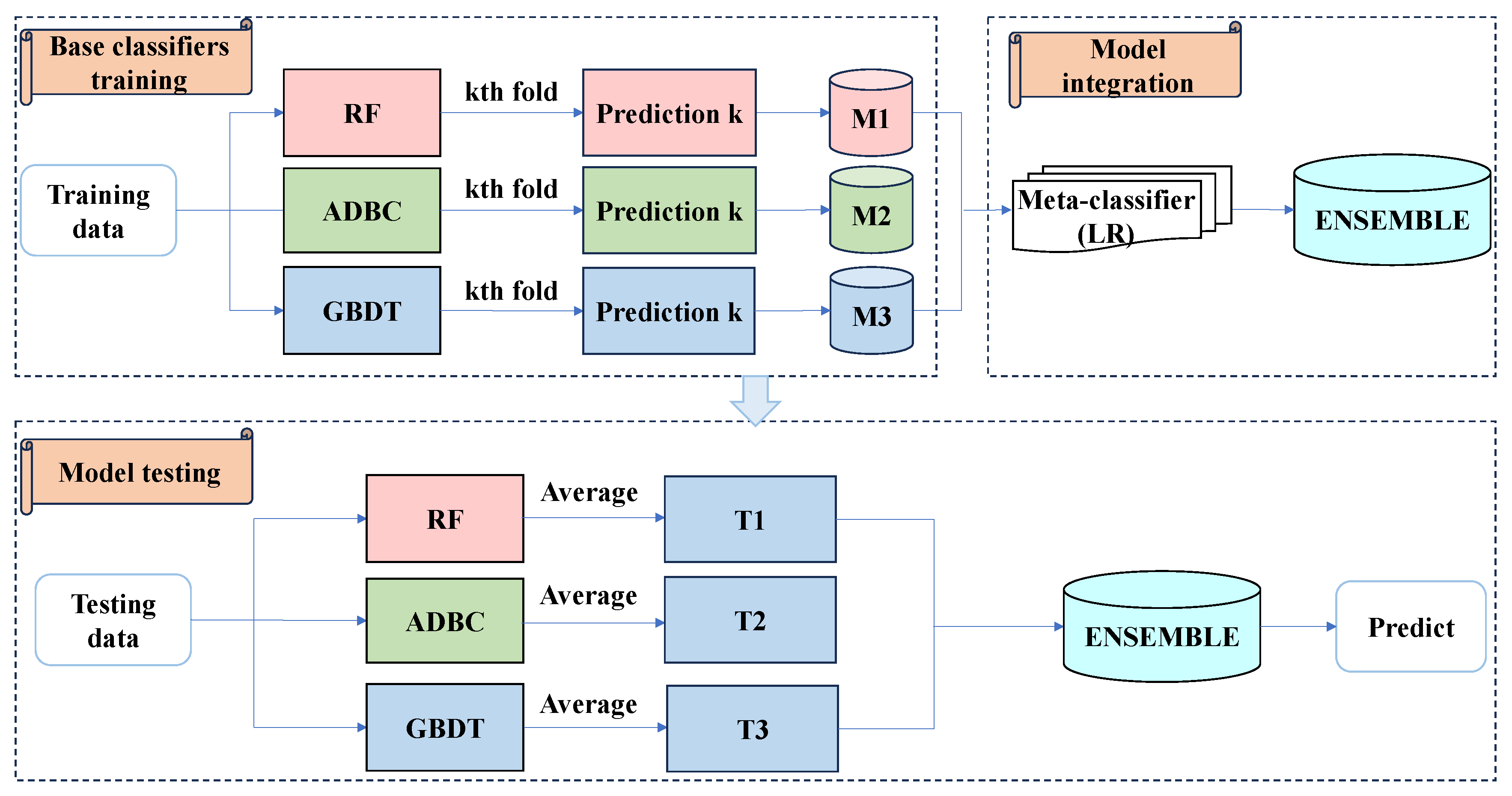
3.3.5. Ensemble Modeling

Ensemble models create more powerful learners by combining multiple base learners to produce more accurate model predictions [54,55]. Bagging and boosting ensemble methods combine the same types of models (e.g., decision trees) to reduce instability or bias in a single model, while stacking and blending two algorithms typically integrate different types of models, exploiting the strengths of different models and minimizing their weaknesses to achieve better performance [18]. The ensemble learning method used in this paper is the stacked ensemble learning method [56], which synthesizes several algorithms (regression or classification) during the training phase. In this study, the first step is to train the basic classifier models RF, ADBC, and GBDT; the second step is to synthesize the output features of the three basic classifiers to generate a new set of training data; finally, the ensemble classifier model is trained using a logistic regression algorithm to superimpose the computational errors of ensemble and estimation on all the basic classifiers, and then these residuals are reduced again through a meta-learning step (Figure 4).

3.4. Model Evaluation Metrics

To evaluate the performance of the flood sensitivity model, this study used two different methods, namely the area under the receiver operating characteristic curve (ROC-AUC) and the statistical measure to evaluate the performance of the model. The closer the AUC (area under the curve) value is to 1, the better the model performance [11]. Another method is to evaluate and compare the performance of the model by calculating four indicators: accuracy, precision, recall, and F1 score [14]. These statistical indicators help to check whether high-precision models are overfitting and to further screen out high-precision models that are in line with real research.
A cc = T P + T N T P + F P + T N + F N
Pr e = T P T P + F P
Re c = T P T P + F N
F 1 = 2 × Pr e × Re c Pr e + Re c
where TP represents a true positive, TN represents a true negative, FP represents a false positive, and FN represents a false negative. In this classification, flooded areas are defined as positive samples, and unflooded areas are defined as negative samples.

3.5. Interpretability Analysis

Interpretability refers to understanding the output of a black box model based on an interpretable model [57]. Machine learning algorithms developed by Lundberg and Lee open up new avenues for understanding model output [58], providing more transparency to what are often considered black box models. While generally simple models can be interpreted very accurately, machine learning models are more complex in structure and require separate interpretation models to analyze the relationship between model outputs and inputs. Recent research on geological hazards has shown that interpretable models greatly facilitate the understanding of model results [59]. Explainable models include Locally Explainable Models (LIMEs) [60], Neural Supported Decision Trees (NBDTs) [61], and SHAP models [58]. Shapley was originally introduced as a game theory model proposed by Professor Lloyd Shapley to solve the problem of distribution of contributions and payoffs among individual players in cooperative games [62]. In machine learning models, Shapley is used to quantify the contribution of each input feature to the specific prediction of a machine learning model, helping to uncover key input factors in the model’s decision-making process.

3.6. Model Validation

In order to test the reliability of the flood hazard maps generated by the RF, ADBC, GBDT, and ENSEMBLE algorithms, the Seed cell area index (SCAI) was introduced and combined with flood sampling point data to analyze the hazard maps graded according to the level of hazard. The method of calculating the index is as follows [63]:
S C A I = A r e a   e x t e n t   of   s u s c e p t i b i l i t y   c l a s s   % F l o o d   i n   e a c h   s u s c e p t i b i l i t y   c l a s s   %
The degree of flood vulnerability has the opposite relationship to the SCAI, i.e., the higher the degree of vulnerability, the lower the SCAI.

4. Result

4.1. Influence Factor Correlation Analysis

To avoid strong correlations among influence factors that may lead to overfitting in the flood susceptibility model simulation, this study employs Pearson correlation coefficients, TOL, and VIF metrics to identify whether multicollinearity exists among the 11 influence factors. Figure 5 presents the Pearson correlation coefficients among the influence factors; values greater than 0.7 indicate a significant degree of multicollinearity [64]. The highest positive correlation is found between elevation and distance to the river, with a correlation coefficient of 0.52, while the correlation coefficient between SPI and slope is 0.50. Conversely, the highest negative correlation is observed between distance to river and drainage density, with a coefficient of −0.60, and the correlation between elevation and drainage density is −0.53 (Figure 5). All Pearson correlation coefficients among the influence factors are below 0.7, indicating no strong correlations among the selected factors. Table 2 shows the results of the multicollinearity analysis, with the lowest tolerance value being for drainage density (0.541), which exceeds the theoretical threshold of 0.10 [26]. Additionally, the maximum VIF value is 1.819, and all variables have VIF values below the multicollinearity threshold of 10.00 [26,65]. Therefore, the influence factor variables selected in this study meet the criteria of TOL greater than 0.1, VIF less than 10, and all pairwise correlation coefficients below 0.7, indicating that there is no significant multicollinearity among the selected influence factors, which can be used as input data for the model.

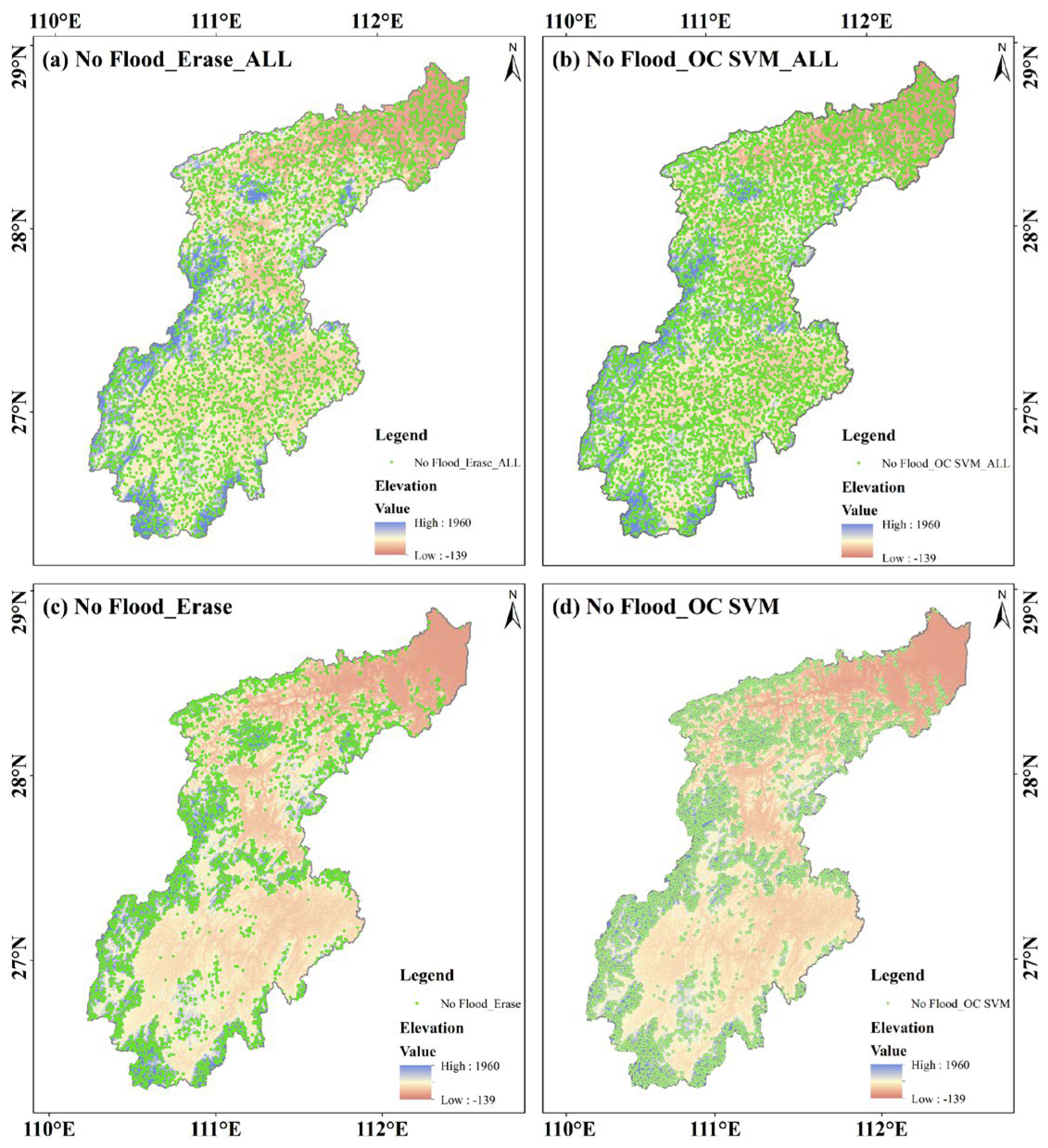
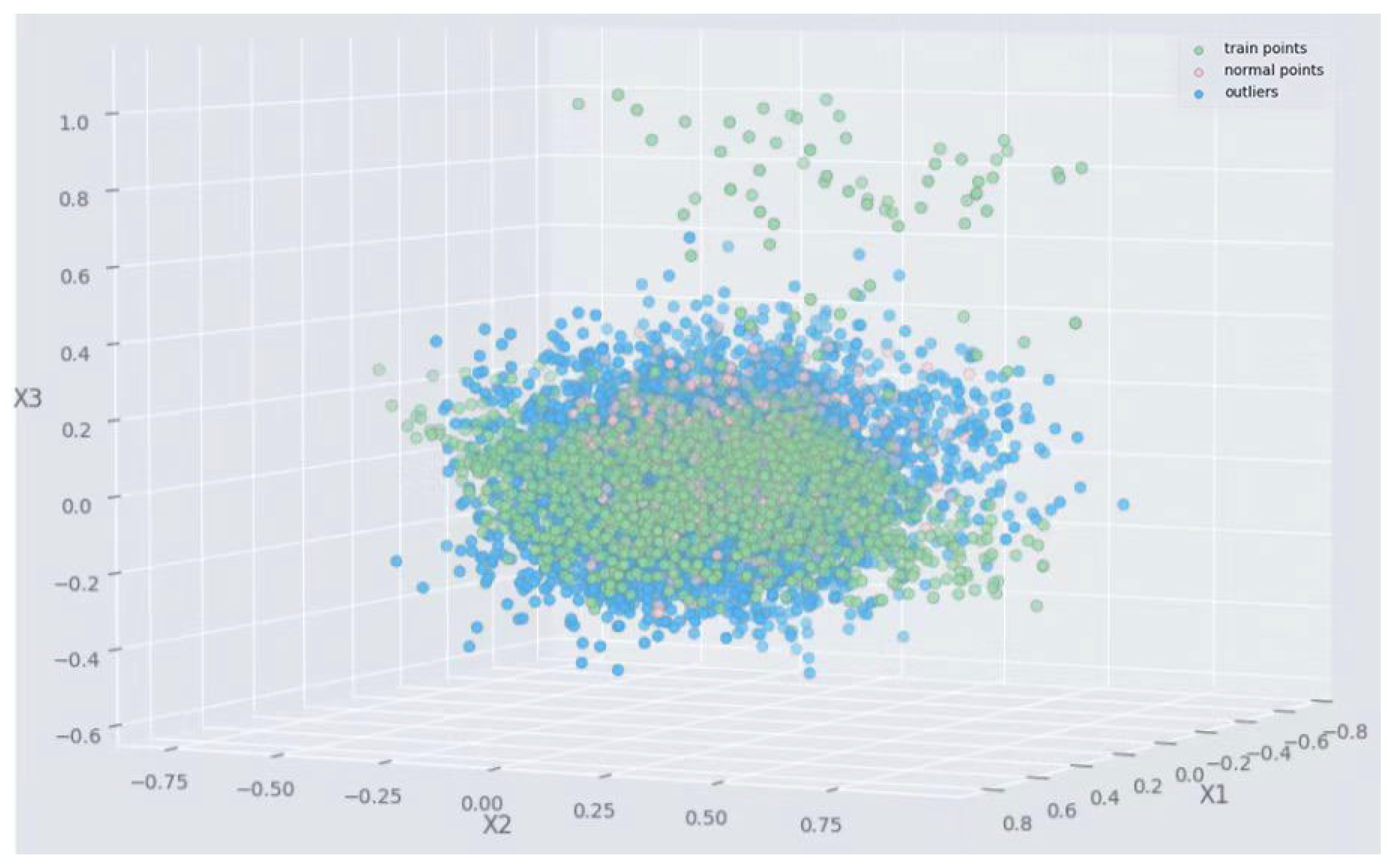
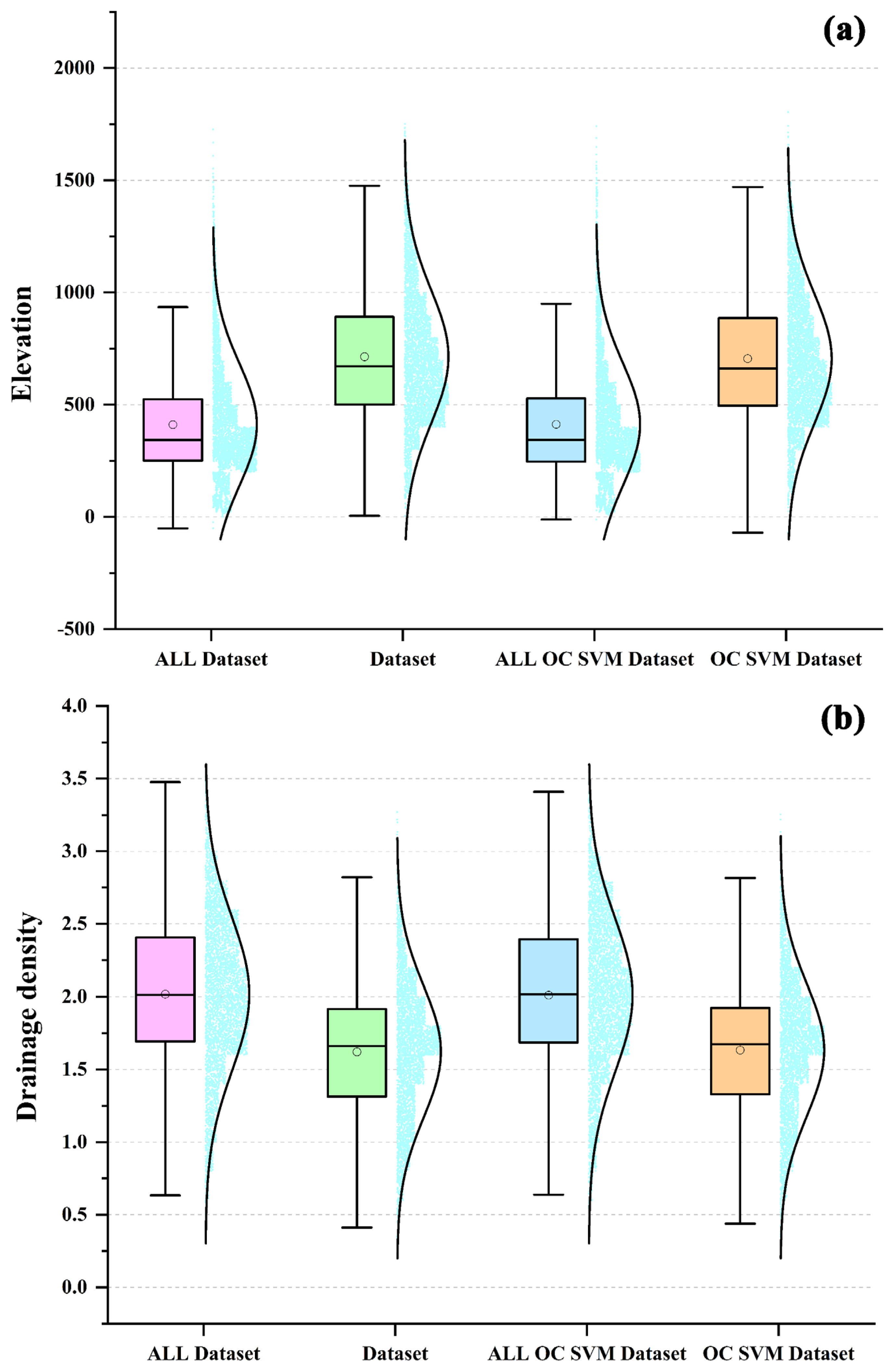
4.2. Non-Flood Point Dataset Extraction

The flood point and non-flood point datasets contain spatial location information, serving as the basis for the flood susceptibility model to generate flood susceptibility maps for the study area based on the characteristics of flood influencing factors. However, flood points used as positive samples in the model can be obtained through field surveys, remote sensing interpretation during flood inundation, and historical flood cataloging, resulting in relatively high data quality. In contrast, non-flood points, used as negative samples in the model, cannot be accurately obtained, leading to greater uncertainty in the flood susceptibility model’s simulation results.
As shown in Figure 6, the study uses range constraints and algorithm constraints to extract non-flood sample data. We first selected the initial non-flood dataset non-flood points1-1 in the study area. Combined with the frequency ratio algorithm to determine the low and low susceptibility areas, non-flood points1-2 was selected as the second initial non-flood sample set (Figure 6). Then, the buffer algorithm and OC SVM algorithm were used to eliminate potential flood points in the two initial non-flood sample datasets. The 500 m buffer algorithm is used to eliminate possible non-flood points. The OC SVM algorithm further screens out non-flood samples with similar environmental factors to flood samples by analyzing flood samples and their environmental factor data, ensuring that the final non-flood sample dataset is accurate and reliable.
This study utilized a sample set of 3364 flood points based on the flood inventory map to obtain four non-flood point datasets through spatial range and sampling methods. Non-flood point dataset I (ALL Dataset): Non-flood points were randomly selected using the buffer method within the remaining study area after excluding flood points (Figure 7a). Non-flood point dataset II (Dataset): Non-flood points were randomly selected using the buffer method within the lower and low flood susceptibility level ranges identified by the frequency ratio statistical model (Figure 7c). Non-flood point dataset III (ALL OC SVM Dataset): Non-flood points were randomly selected using the OC SVM method within the remaining study area after excluding flood points (Figure 7b). Non-flood point dataset IV (OC SVM Dataset): Non-flood points were randomly selected using the OC SVM method within the lower and low flood susceptibility level ranges identified by the frequency ratio statistical model (Figure 7d). In addition, the buffer distance used in the buffer method in this study was 500 m.

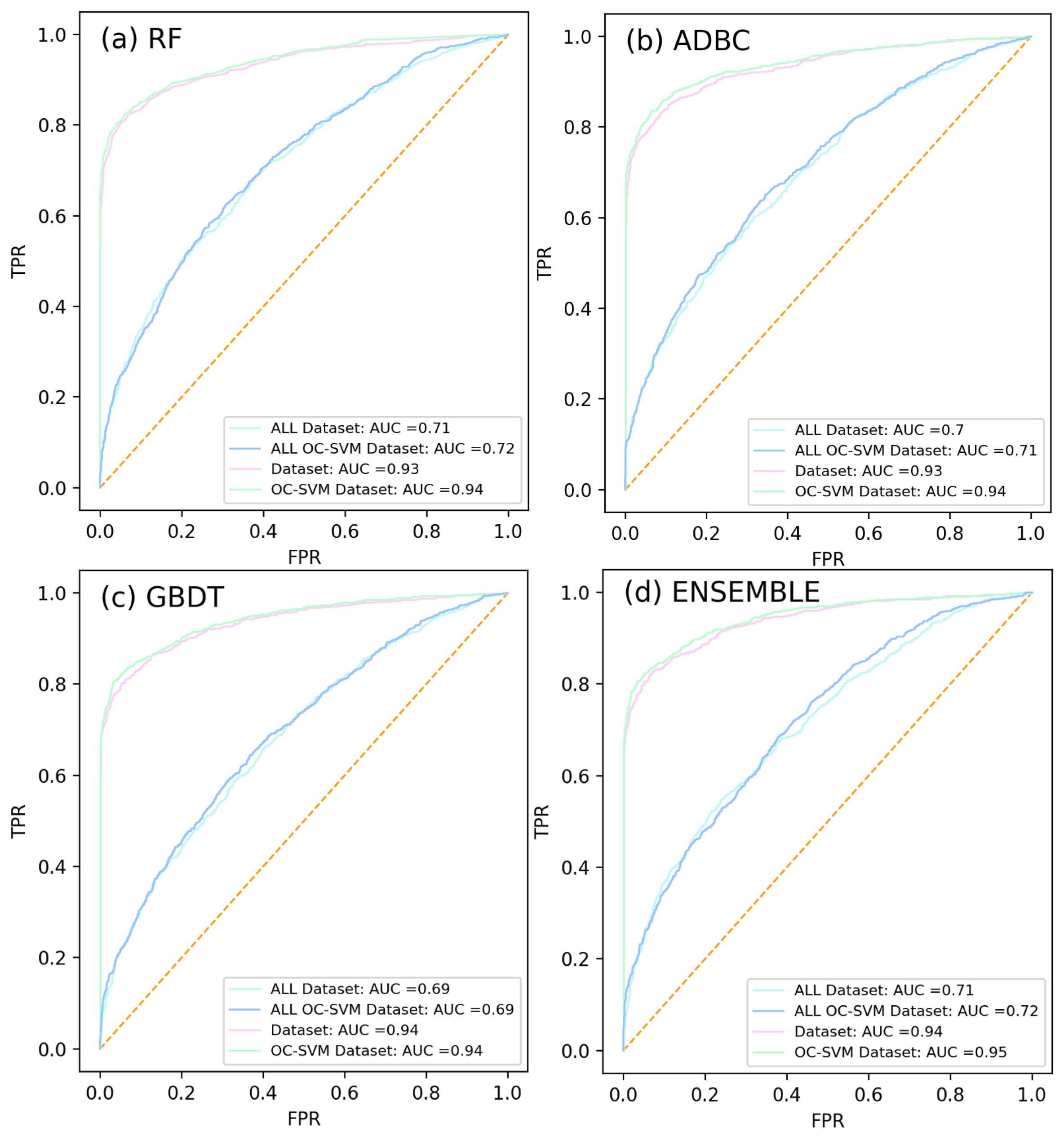
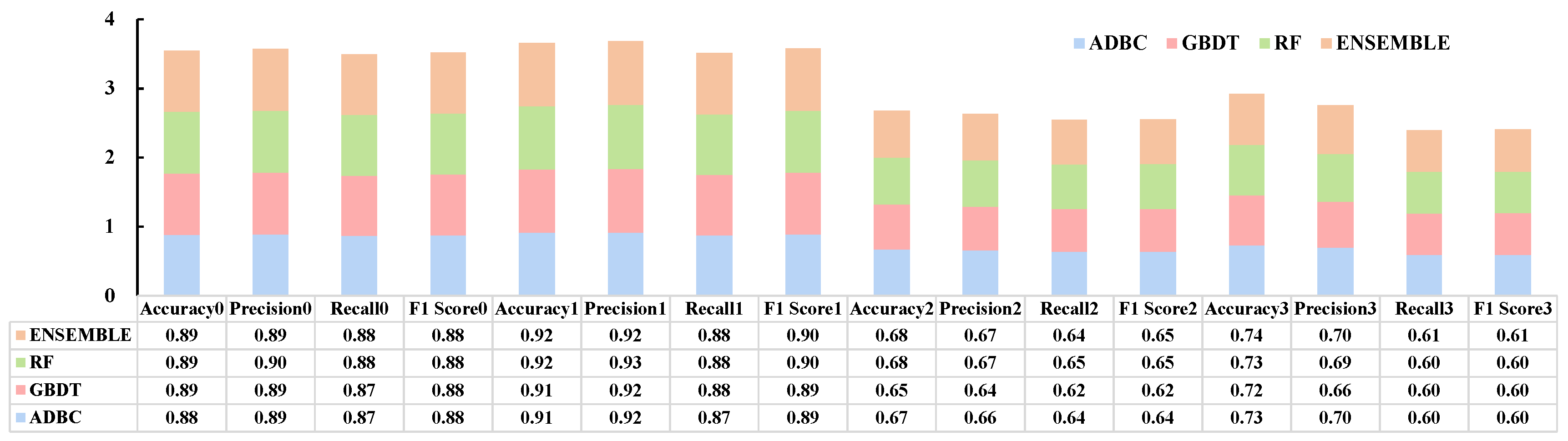
4.3. Accuracy Evaluation of the Model Based on Non-Flood Point Dataset

This study uses Random Forest (RF), Adaptive Boosting (ADBC), Gradient Boosting Decision Tree (GBDT), and stacking ensemble learning (ENSEMBLE) to construct flood susceptibility models. The model input data consist of flood points, influencing factors, and four types of non-flood points, using ROC curves (Figure 8) and metrics like accuracy, precision, recall, and F1 score (Figure 9) to analyze the effect of the four non-flood point sampling methods on the simulation accuracy of flood susceptibility. The results indicate that the ensemble model outperforms individual models in goodness of fit and generalization capability, and optimizing the extraction range of non-flood point datasets can significantly improve the accuracy of flood susceptibility results. The ROC curve values for the ENSEMBLE model, using four types of non-flood point datasets, are generally the highest, with ROC values for non-flood point datasets I to IV at 0.71, 0.72, 0.94, and 0.95, respectively. Furthermore, the ENSEMBLE model has the highest overall values for accuracy, precision, recall, and F-1 score, showing that it is the best model for simulating flood susceptibility among the four models. For the ENSEMBLE model, the accuracy of non-flood point datasets II (0.94) and IV (0.95) is significantly higher than that of datasets I (0.71) and III (0.72), suggesting that the range determined by the frequency ratio model is preferable to the study area range. Most flood susceptibility model studies have also proved that the accuracy of the integrated model is higher than that of a single model [18,66], so the integrated model is mainly used for analysis in the study.
Figure 10 illustrates the OC SVM algorithm’s results in filtering potential flood points, where green points denote known flood samples, and blue points indicate non-flood samples with environmental characteristics that differ substantially from flood samples. Red sample points, having environmental factor values similar to known flood samples, are potential flood points within the non-flood sample dataset. The OC SVM algorithm increases the accuracy of the non-flood dataset by learning environmental characteristics from flood points, thereby excluding potential flood points (red points) and identifying potential non-flood points (blue points) within the dataset.

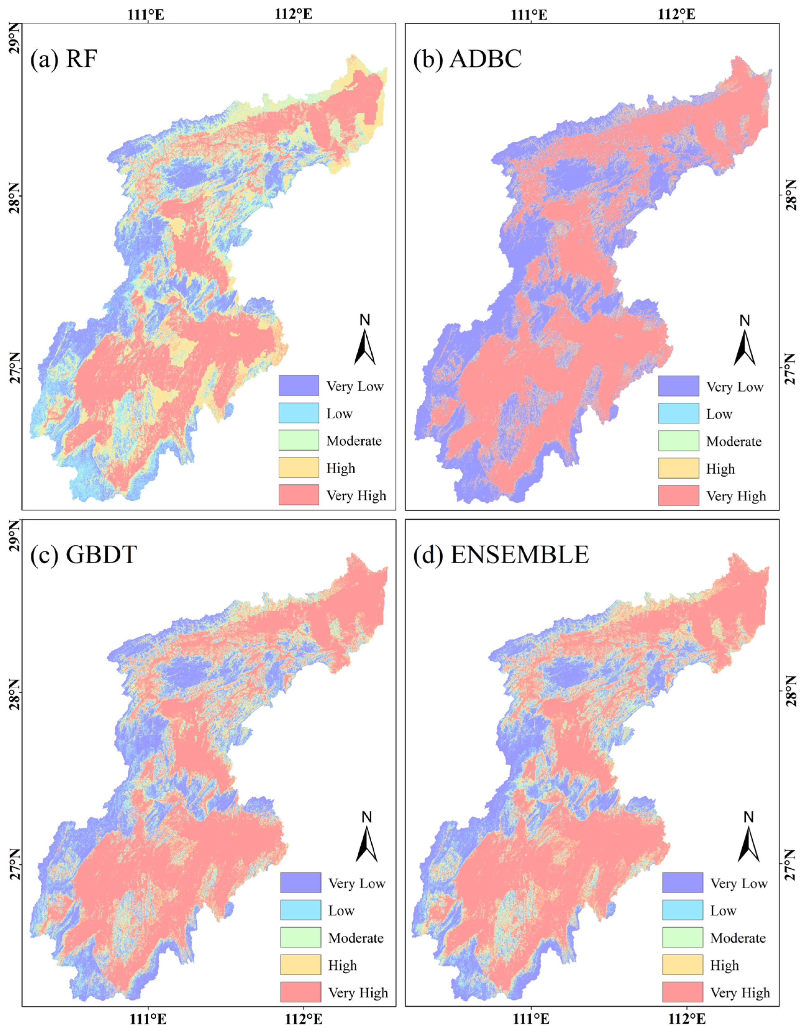
4.4. The Flood Susceptibility Map

The flood susceptibility map shows the likelihood of flooding at a given location based on relevant influencing factors. In this study, the highest accuracy non-flood point dataset IV (OC SVM Dataset) was used as an input to four flood susceptibility models to calculate flood susceptibility. The study results were classified in ArcGIS 10.7 using the natural breaks method, categorizing flood susceptibility into five risk levels: very high, high, medium, low, and very low (Figure 11). The natural breaks method identifies classification intervals in the data, groups similar values, and sets boundaries where the data values are widely different. The high flood susceptibility simulated by the four models is mainly concentrated in the northeastern and southeastern regions, which are characterized by low elevation and high drainage density.
To further analyze the flood susceptibility map, this study calculated the pixel count for each flood susceptibility level predicted by the four models and obtained the proportion of each flood susceptibility level (Figure 12). With an increase in susceptibility level, the pixel count for each level first decreases and then increases, with very low and very high susceptibility areas showing a higher proportion. In the ENSEMBLE model, the spatial coverage for areas of very low, low, medium, high, and very high flood susceptibility is 5600 km2 (20%), 2772 km2 (10%), 2201 km2 (8%), 3139 km2 (11%), and 14,018 km2 (51%), respectively. The flood susceptibility model using non-flood point dataset IV as an input in the ENSEMBLE model achieved the highest accuracy evaluation (95%).
Model predictions of flood susceptibility indicate extremely high flood susceptibility in Ziyang District, Shuangqing District, Beita District, Daxiang District, and Shaoyang County in Hunan Province, with relatively high susceptibility in Taojiang, Anhua, and Wugang City. Lower flood susceptibility areas are primarily located in Suining County, the northwest of Longhui County, and the west of Dongkou County. In general, the flood risk in the Zijiang River Basin shows a polarized trend, with a significant proportion of extremely high and extremely low susceptibility areas. The local government urgently needs to manage high susceptibility areas to mitigate flood damage. Furthermore, based on the SCAI calculation results (Table 3), the SCAI values for flood susceptibility levels in the RF, ADBC, GBDT, and ENSEMBLE models increase as susceptibility levels decrease, indicating that the flood susceptibility models used in this study are reliable for flood-prone area prediction.

4.5. Model Interpretability

To analyze the impact of influencing factors on flood susceptibility, Figure 13 shows the SHAP plots for RF, ADBC, GBDT, and ENSEMBLE. The vertical axis ranks influencing factors by importance from low to high, while the horizontal axis represents the Shapley value, with positive and negative values indicating whether the influence on susceptibility is positive or negative. Elevation and drainage density are significant influencing factors in all four models, while curvature has the least effect on flood susceptibility. High values in the elevation factor (shown as red points) correspond to negative Shapley values, discouraging flood occurrence. Due to higher elevation in the southwestern study area, the model predicts lower flood susceptibility levels in this region (Figure 11). In contrast, drainage density influences flood susceptibility in the opposite manner, with high drainage density values promoting frequent flooding. Lower elevation and higher drainage density in the northern and southeastern study area result in higher flood susceptibility (Figure 11). In addition to elevation and drainage density, slope, aspect, vegetation index, and land use are also significant influencing factors for flood susceptibility in the region (Figure 13d). Land use influences the extent of permeable surfaces and vegetation cover, affecting infiltration rates and runoff. Moreover, land use changes alter soil hydrological properties (e.g., permeability), thereby impacting flood susceptibility.
Agricultural and built-up land types are crucial to human life and are more likely to lead to flood disasters [67,68]. Therefore, this study analyzed the relationship between flood susceptibility levels in the ENSEMBLE flood susceptibility map and the factors of agricultural and built-up land use in the land use type influencing factors (Figure 14). The results indicate that the proportion of agricultural and built-up land areas in high susceptibility levels have the largest, at 85.6% and 94.2%, respectively, while in very low susceptibility areas, the proportion is only 1.2% and 0.1%. The smaller the proportion of agricultural and built-up land area, the lower the flood risk. The higher the footprint of cultivated land and building land, the higher the susceptibility level, and the higher the impact on flood occurrence to some extent, consistent with previous research results [69]. Cultivated and built-up land is mostly located at lower elevation. Therefore, in this study, we carried out a further analysis of the effects of low elevation and cropland and building land on flood vulnerability. The distribution of elevation of cropland and building land among land use types in the study area was analyzed, and it was found that cropland was located at an average elevation of 393.73 m and building land was located at an average elevation of 236.26 m, which were in the low elevation area. Elevation is a significant factor influencing the occurrence of flooding, and in low elevation areas, areas of cropland and built-up land further exacerbate the likelihood of flooding. Therefore, due to the influence of agricultural and built-up land area proportions in the Zijiang River Basin, the area proportions of extremely low and extremely high flood susceptibility in the study area exhibit an extreme distribution trend.

5. Discussion

5.1. Uncertainty Analysis of Non-Flood Sample Selection

In order to further analyze the impact of non-flood sample selection methods on flood susceptibility simulation results, this study used cloud–rain maps to analyze the distribution of predicted values of different non-flood samples in the integrated model (Figure 15). Non-flood sample datasets I and III produced higher flood susceptibility prediction values, with a median of 0.87. Based on the frequency ratio algorithm to determine the non-flood sample selection range (datasets II and IV), the flood susceptibility prediction values of non-flood samples selected within the range were mainly lower than 0.2. Moreover, the flood susceptibility prediction value of non-flood samples dataset IV selected by the OC SVM algorithm was the lowest. This shows that the non-flood point extraction range determined by the frequency ratio algorithm and the non-flood samples selected by the OC SVM algorithm are of higher quality, which can better reflect the spatial location distribution of non-floods and improve the accuracy of model simulation.
Box plots were also used to evaluate the distribution of different non-flood samples in flood influencing factors (Figure 16). Figure 16 shows the distribution of non-flood samples based on elevation and drainage density. The distribution of elevation data on the four non-flood point datasets shows that the mean elevation values of non-flood point datasets II and IV are much higher than those of non-flood point datasets I and III, and higher elevation values do not take advantage of the occurrence of floods (Figure 16a). The non-flood point dataset IV is concentrated in distribution, with a large degree of aggregation, and the mean is lower than the mean of drainage density of non-flood point datasets I and III (Figure 16b). Figure 13 shows that the higher drainage density is in the flood occurrence area. This study indicates that the non-flood points selected based on the frequency ratio algorithm and the OC SVM algorithm have better regularity and stronger rationality. This effectively avoids the problems of randomness and uncertainty that exist in other methods.
Flood susceptibility models using machine learning algorithms have been extensively applied in flood susceptibility research [4,27], but reducing the uncertainty in flood susceptibility maps remains a challenging task. Therefore, this study explores and proposes an optimal method based on spatial scope and sampling strategy to reduce uncertainty in non-flood point datasets, thereby achieving accurate large-scale flood susceptibility maps. Randomly selecting non-flood points within the excluded flood point dataset range reduces human interference to some extent, has acceptable predictive accuracy, and is easy to implement. Previous studies have mostly used this approach to select non-flood point datasets [13]. However, this method does not consider the possibility of high-susceptibility samples in areas without historical flood records, which may impact the quality and reliability of non-flood samples [70].
The buffer method can reduce the error rate of selected negative samples. This study compared prediction results for different buffer distances and found that a 500 m buffer distance is optimal. The optimal buffer distance used in the study depends on local environmental characteristics and data sources and requires multiple trials for accurate determination [71]. Furthermore, buffer distances vary significantly across different study areas. Lucchese et al. found a 1 km buffer distance to be suitable [71], whereas Miao et al. suggested an optimal buffer distance of 200–500 m [72]. However, if the buffer distance is fixed, it restricts the spatial range for selecting non-landslide samples, resulting in uneven sample distribution (Figure 7c,d).
To solve the issues in negative sample selection methods, this study utilizes the frequency ratio model and OC SVM approach to achieve more efficient and accurate selection of non-flood samples. Based on accuracy evaluation results, it is evident that the combination of the frequency ratio model and OC SVM method has higher predictive accuracy compared to the other three methods (Figure 7d). Ye et al. also demonstrated that a negative sample dataset obtained using the OC SVM method enhances the performance of landslide models [31]. The OC SVM method captures the relationship between flood sample distribution and environmental features, which improves the quality of training and testing sets, enhances model prediction accuracy, and reduces modeling uncertainty. However, beyond the spatial range and methods of non-flood point sampling, the ratio of flood–non-flood sample numbers can also impact flood susceptibility, making it a direction worthy of attention [24]. This study focuses on examining the effects of non-flood sample sampling range and methods on flood susceptibility, and further research is needed to determine the appropriate ratio of flood–non-flood samples. Furthermore, factors such as grid size, the quality and quantity of flood influencing factors, and the type of algorithm also influence flood susceptibility maps.

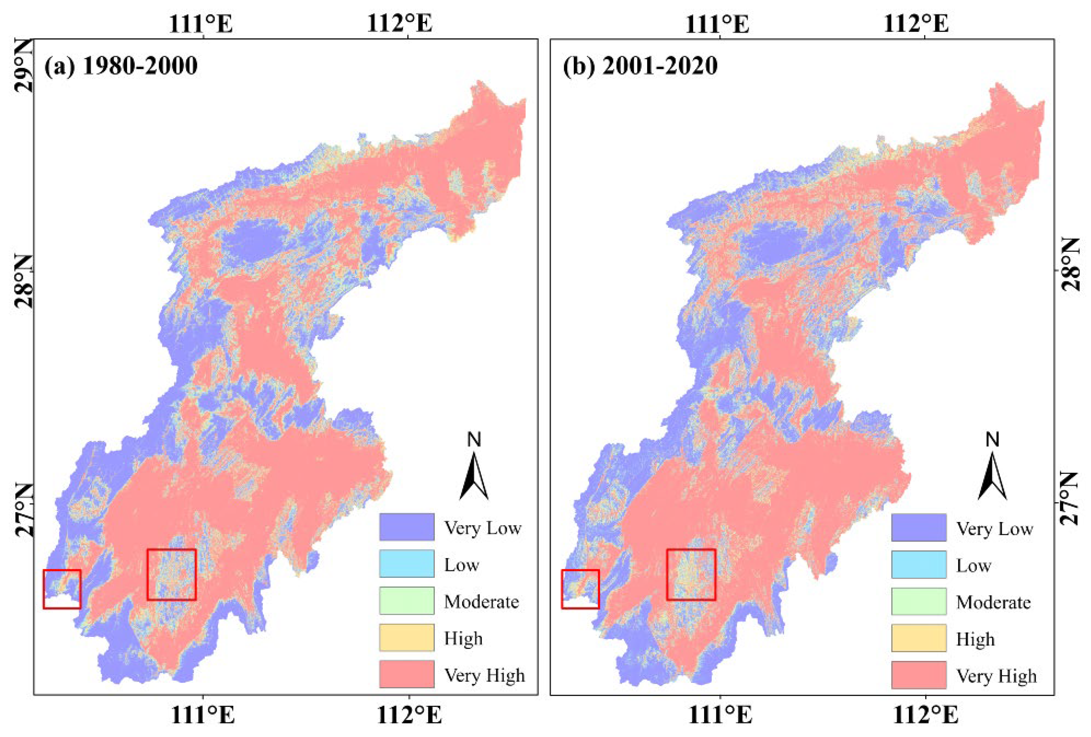
5.2. Dynamic Analysis of Flood Susceptibility

In order to dynamically reflect the spatial distribution of flood susceptibility in the Zijiang River Basin, the study selected land use type data in 2000 and 2020 to characterize land use type changes and used multi-year average rainfall data from 1980 to 2000 (before 2000) and 2001 to 2020 (after 2000) to characterize climate change. The optimal non-flood point dataset and the constructed ENSENMBLE integrated model were used to simulate the flood susceptibility map of the Zijiang River Basin before and after 2000 (Figure 17). The simulation accuracy of the ENSENMBLE model before and after 2000 is 0.94 and 0.95, respectively, indicating high accuracy and reliable simulation results. In order to compare and analyze the changes in flood susceptibility levels in the Zijiang River Basin in two periods, this study used the same classification interval to classify the susceptibility results, taking the natural break point classification interval of the flood susceptibility results before 2000 as the standard.
It can be clearly seen from Figure 17 that the flood susceptibility in the southwest of the Zijiang River Basin increased significantly after 2000. By comparing and analyzing the changes in flood susceptibility risk levels before and after 2000, it is found (Figure 18) that the area that changed from level IV (high flood susceptibility risk level) before 2000 to level V (very high flood susceptibility risk level) after 2000 accounted for as high as 76.2%. The areas where the flood susceptibility levels of level III (moderate flood susceptibility risk level), level II (low flood susceptibility risk level), and level I (very low flood susceptibility risk level) changed to level V accounted for 16.1%, 6.0%, and 1.7%, respectively.
Compared with 1980–2000, the newly added area of very high flood susceptibility areas after 2000 was 861.5 km2, and the area converted from high flood susceptibility to very high flood susceptibility accounted for 656.6 km2, of which the cultivated land and building land areas in the newly added very high flood susceptibility areas were 443.0 km2 and 12.6 km2, respectively. Among the newly added very high flood susceptibility areas, the area converted from forest land to cultivated land was 147.6 km2, accounting for 22.4%. In addition, the area converted from non-building land to building land was 5.9 km2, accounting for 0.9%. Moreover, among the newly added areas with very high flood susceptibility, the area with an increase in average annual rainfall after 2000 is 17.9 km2, accounting for only 2.7%. This indicates that land use changes after 2000 have significantly increased the flood susceptibility risk level in the Zijiang River Basin, while climate change caused by rainfall has a lower impact on the very high flood susceptibility risk level in the Zijiang River Basin than land use changes.

6. Conclusions

Flooding is one of the most destructive natural disasters in the Zijiang River Basin, and disaster managers urgently need to map flood susceptibility across the basin to minimize severe losses of life and property. This study aims to establish an optimal approach for enhancing flood susceptibility mapping by reducing the non-flood point dataset. The conclusions are as follows:
(1) Optimizing the spatial range and sampling method for selecting non-flood datasets can improve model prediction accuracy. In low and very low flood susceptibility areas determined by the frequency ratio algorithm, using OC SVM sampling to obtain non-flood samples significantly enhances flood susceptibility simulation accuracy. Compared to using the buffer method within the study area, model accuracy increased by 23% (RF), 24% (ADBC and ENSEMBLE), and 25% (GBDT).
(2) The ENSEMBLE model surpasses individual models in goodness of fit and generalization ability. When using the optimal non-flood dataset IV as the negative sample input, the ENSEMBLE model achieves a maximum AUC of 0.95 for flood susceptibility modeling. Flood susceptibility is higher in the northern and southeastern regions of the study area, with lower susceptibility in the southwestern part due to higher elevation. Flood risk levels in the Zijiang River Basin show a polarized distribution pattern.
(3) The Shap explainable model reveals that elevation, slope, and drainage density are the three most important influencing factors. Areas with low elevation and low slope are high flood susceptibility zones, while low drainage density is unfavorable for flood occurrence.

Author Contributions

Conceptualization, R.Y.; Methodology, Y.Z., R.Y. and P.S.; Formal analysis, Y.Z. and Y.W.; Investigation, Y.Z., N.Z. and X.X.; Data curation, P.S.; Writing–original draft, Y.Z.; Writing–review & editing, R.Y.; Visualization, Y.W., N.Z. and X.X.; Supervision, R.Y. and P.S.; Funding acquisition, R.Y. and P.S. All authors have read and agreed to the published version of the manuscript.

Funding

This work was financially supported by the National Science Foundation of China (Grant No. 42271037), the National Science Foundation of Anhui province, China (Grant No. 2408085MD095), Key Research and Development Program Project of Anhui province, China (Grant No. 2022m07020011), the University Synergy Innovation Program of Anhui Province, China (Grant No. GXXT-2021-048), and Science Foundation for Excellent Young Scholars of Anhui, China (Grant No. 2108085Y13).

Data Availability Statement

The raw data supporting the conclusions of this article will be made available by the authors on request.

Conflicts of Interest

The authors declare that they have no known competing financial interests or personal relationships that could have appeared to influence the work reported in this paper.

References

  1. Shahiri Tabarestani, E.; Afzalimehr, H. A comparative assessment of multi-criteria decision analysis for flood susceptibility modelling. Geocarto Int. 2022, 37, 5851–5874. [Google Scholar] [CrossRef]
  2. Chen, J.; Shi, X.; Gu, L.; Wu, G.; Su, T.; Wang, H.-M.; Kim, J.-S.; Zhang, L.; Xiong, L. Impacts of climate warming on global floods and their implication to current flood defense standards. J. Hydrol. 2023, 618, 129236. [Google Scholar] [CrossRef]
  3. Shah, S.A.; Ai, S. Flood susceptibility mapping contributes to disaster risk reduction: A case study in Sindh, Pakistan. Int. J. Disaster Risk Reduct. 2024, 108, 104503. [Google Scholar] [CrossRef]
  4. Islam, A.R.M.T.; Talukdar, S.; Mahato, S.; Kundu, S.; Eibek, K.U.; Pham, Q.B.; Kuriqi, A.; Linh, N.T.T. Flood susceptibility modelling using advanced ensemble machine learning models. Geosci. Front. 2021, 12, 101075. [Google Scholar] [CrossRef]
  5. Zennaro, F.; Furlan, E.; Simeoni, C.; Torresan, S.; Aslan, S.; Critto, A.; Marcomini, A. Exploring machine learning potential for climate change risk assessment. Earth-Sci. Rev. 2021, 220, 103752. [Google Scholar] [CrossRef]
  6. Gharbi, M.; Soualmia, A.; Dartus, D.; Masbernat, L. Comparison of 1D and 2D hydraulic models for floods simulation on the Medjerda Riverin Tunisia. J. Mater. Environ. Sci. 2016, 7, 3017–3026. [Google Scholar]
  7. Chen, R.; Han, B.; Zhao, L.; Zhang, Y.; Cao, Y. Study on water disaster risk of Majiahe River Watershed in Puyang City under extreme rainfall. Water Resour. Hydropower Eng. 2022, 53, 34–43. [Google Scholar]
  8. Abbott, M.B.; Bathurst, J.C.; Cunge, J.A.; O’Connell, P.E.; Rasmussen, J. An introduction to the European Hydrological System—Systeme Hydrologique Europeen,“SHE”, 1: History and philosophy of a physically-based, distributed modelling system. J. Hydrol. 1986, 87, 45–59. [Google Scholar] [CrossRef]
  9. Buahin, C.A.; Horsburgh, J.S. Evaluating the simulation times and mass balance errors of component-based models: An application of OpenMI 2.0 to an urban stormwater system. Environ. Model. Softw. 2015, 72, 92–109. [Google Scholar] [CrossRef]
  10. Shrestha, N.K.; Leta, O.T.; De Fraine, B.; Van Griensven, A.; Bauwens, W. OpenMI-based integrated sediment transport modelling of the river Zenne, Belgium. Environ. Model. Softw. 2013, 47, 193–206. [Google Scholar] [CrossRef]
  11. Youssef, A.M.; Mahdi, A.M.; Pourghasemi, H.R. Optimal flood susceptibility model based on performance comparisons of LR, EGB, and RF algorithms. Nat. Hazards 2023, 115, 1071–1096. [Google Scholar] [CrossRef]
  12. Tehrany, M.S.; Pradhan, B.; Jebur, M.N. Flood susceptibility mapping using a novel ensemble weights-of-evidence and support vector machine models in GIS. J. Hydrol. 2014, 512, 332–343. [Google Scholar] [CrossRef]
  13. Seydi, S.T.; Kanani-Sadat, Y.; Hasanlou, M.; Sahraei, R.; Chanussot, J.; Amani, M. Comparison of machine learning algorithms for flood susceptibility mapping. Remote Sens. 2022, 15, 192. [Google Scholar] [CrossRef]
  14. Lyu, H.M.; Yin, Z.Y. Flood susceptibility prediction using tree-based machine learning models in the GBA. Sustain. Cities Soc. 2023, 97, 104744. [Google Scholar] [CrossRef]
  15. Wang, Y.; Fang, Z.; Hong, H.; Peng, L. Flood susceptibility mapping using convolutional neural network frameworks. J. Hydrol. 2020, 582, 124482. [Google Scholar] [CrossRef]
  16. Wang, Y.; Fang, Z.; Wang, M.; Peng, L.; Hong, H. Comparative study of landslide susceptibility mapping with different recurrent neural networks. Comput. Geosci. 2020, 138, 104445. [Google Scholar] [CrossRef]
  17. Bui, Q.T.; Nguyen, Q.H.; Nguyen, X.L.; Pham, V.D.; Nguyen, H.D.; Pham, V.M. Verification of novel integrations of swarm intelligence algorithms into deep learning neural network for flood susceptibility mapping. J. Hydrol. 2020, 581, 124379. [Google Scholar] [CrossRef]
  18. Yao, J.; Zhang, X.; Luo, W.; Liu, C.; Ren, L. Applications of Stacking/Blending ensemble learning approaches for evaluating flash flood susceptibility. Int. J. Appl. Earth Obs. Geoinf. 2022, 112, 102932. [Google Scholar] [CrossRef]
  19. Dou, J.; Yunus, A.P.; Bui, D.T.; Merghadi, A.; Sahana, M.; Zhu, Z.; Chen, C.W.; Han, Z.; Pham, B.T. Improved landslide assessment using support vector machine with bagging, boosting, and stacking ensemble machine learning framework in a mountainous watershed, Japan. Landslides 2020, 17, 641–658. [Google Scholar] [CrossRef]
  20. Chen, W.; Panahi, M.; Tsangaratos, P.; Shahabi, H.; Ilia, I.; Panahi, S.; Li, S.; Jaafari, A.; Ahmad, B.B. Applying population-based evolutionary algorithms and a neuro-fuzzy system for modeling landslide susceptibility. Catena 2019, 172, 212–231. [Google Scholar] [CrossRef]
  21. Chen, W.; Hong, H.; Li, S.; Shahabi, H.; Wang, Y.; Wang, X.; Ahmad, B.B. Flood susceptibility modelling using novel hybrid approach of reduced-error pruning trees with bagging and random subspace ensembles. J. Hydrol. 2019, 575, 864–873. [Google Scholar] [CrossRef]
  22. Kanani-Sadat, Y.; Arabsheibani, R.; Karimipour, F.; Nasseri, M. A new approach to flood susceptibility assessment in data-scarce and ungauged regions based on GIS-based hybrid multi criteria decision-making method. J. Hydrol. 2019, 572, 17–31. [Google Scholar] [CrossRef]
  23. Al-Aizari, A.R.; Alzahrani, H.; AlThuwaynee, O.F.; Al-Masnay, Y.A.; Ullah, K.; Park, H.J.; Al-Areeq, N.M.; Rahman, M.; Hazaea, B.Y.; Liu, X. Uncertainty Reduction in Flood Susceptibility Mapping Using Random Forest and eXtreme Gradient Boosting Algorithms in Two Tropical Desert Cities, Shibam and Marib, Yemen. Remote Sens. 2024, 16, 336. [Google Scholar] [CrossRef]
  24. Ekmekcioğlu, Ö.; Koc, K.; Özger, M.; Işık, Z. Exploring the additional value of class imbalance distributions on interpretable flash flood susceptibility prediction in the Black Warrior River basin, Alabama, United States. J. Hydrol. 2022, 610, 127877. [Google Scholar] [CrossRef]
  25. Dou, J.; Yunus, A.P.; Merghadi, A.; Shirzadi, A.; Nguyen, H.; Hussain, Y.; Avtar, R.; Chen, Y.; Pham, B.T.; Yamagishi, H. Different sampling strategies for predicting landslide susceptibilities are deemed less consequential with deep learning. Sci. Total Environ. 2020, 720, 137320. [Google Scholar] [CrossRef]
  26. Tehrany, M.S.; Pradhan, B.; Mansor, S.; Ahmad, N. Flood susceptibility assessment using GIS-based support vector machine model with different kernel types. Catena 2015, 125, 91–101. [Google Scholar] [CrossRef]
  27. Khosravi, K.; Shahabi, H.; Pham, B.T.; Adamowski, J.; Shirzadi, A.; Pradhan, B.; Dou, J.; Ly, H.B.; Gróf, G.; Ho, H.L.; et al. A comparative assessment of flood susceptibility modeling using multi-criteria decision-making analysis and machine learning methods. J. Hydrol. 2019, 573, 311–323. [Google Scholar] [CrossRef]
  28. Wang, Y.; Fang, Z.; Hong, H.; Costache, R.; Tang, X. Flood susceptibility mapping by integrating frequency ratio and index of entropy with multilayer perceptron and classification and regression tree. J. Environ. Manag. 2021, 289, 112449. [Google Scholar] [CrossRef]
  29. MacInnes, J.; Santosa, S.; Wright, W. Visual classification: Expert knowledge guides machine learning. IEEE Comput. Graph. Appl. 2009, 30, 8–14. [Google Scholar] [CrossRef]
  30. Guo, Z.; Tian, B.; Zhu, Y.; He, J.; Zhang, T. How do the landslide and non-landslide sampling strategies impact landslide susceptibility assessment?—A catchment-scale case study from China. J. Rock Mech. Geotech. Eng. 2024, 16, 877–894. [Google Scholar] [CrossRef]
  31. Ye, C.; Tang, R.; Wei, R.; Guo, Z.; Zhang, H. Generating accurate negative samples for landslide susceptibility mapping: A combined self-organizing-map and one-class SVM method. Front. Earth Sci. 2023, 10, 1054027. [Google Scholar] [CrossRef]
  32. Yang, J.; Huang, X. 30 m annual land cover and its dynamics in China from 1990 to 2019. Earth Syst. Sci. Data Discuss. 2021, 2021, 1–29. [Google Scholar]
  33. Yang, H.; Yao, R.; Dong, L.; Sun, P.; Zhang, Q.; Wei, Y.; Sun, S.; Aghakouchak, A. Advancing flood susceptibility modeling using stacking ensemble machine learning: A multi-model approach. J. Geogr. Sci. 2024, 34, 1513–1536. [Google Scholar] [CrossRef]
  34. Torcivia, C.G.; López, N.R. Preliminary Morphometric Analysis: Río Talacasto Basin, Central Precordillera of San Juan, Argentina Advances in Geomorphology and Quaternary Studies in Argentina; Springer: Cham, Switzerland, 2020; pp. 158–168. [Google Scholar]
  35. Rau, P.; Bourrel, L.; Labat, D.; Ruelland, D.; Frappart, F.; Lavado, W.; Dewitte, B.; Felipe, O. Assessing multidecadal runoff (1970–2010) using regional hydrological modelling under data and water scarcity conditions in Peruvian Pacific catchments. Hydrol. Process. 2019, 33, 20–35. [Google Scholar] [CrossRef]
  36. Giovannettone, J.; Copenhaver, T.; Burns, M.; Choquette, S. A statistical approach to mapping flood susceptibility in the Lower Connecticut River Valley Region. Water Resour. Res. 2018, 54, 7603–7618. [Google Scholar] [CrossRef]
  37. Mahmoud, S.H.; Gan, T.Y. Multi-criteria approach to develop flood susceptibility maps in arid regions of Middle East. J. Clean. Prod. 2018, 196, 216–229. [Google Scholar] [CrossRef]
  38. Moore, I.D.; Grayson, R.B. Terrain-based catchment partitioning and runoff prediction using vector elevation data. Water Resour. Res. 1991, 27, 1177–1191. [Google Scholar] [CrossRef]
  39. Ogden, F.L.; Raj Pradhan, N.; Downer, C.W.; Zahner, J.A. Relative importance of impervious area, drainage density, width function, and subsurface storm drainage on flood runoff from an urbanized catchment. Water Resour. Res. 2011, 47. [Google Scholar] [CrossRef]
  40. Wilson, J.P.; Gallant, J.C. (Eds.) Terrain Analysis: Principles and Applications; John Wiley & Sons: Hoboken, NJ, USA, 2000. [Google Scholar]
  41. Merz, R.; Blöschl, G. A process typology of regional floods. Water Resour. Res. 2003, 39. [Google Scholar] [CrossRef]
  42. Lin, L.; Wu, Z.; Liang, Q. Urban flood susceptibility analysis using a GIS-based multi-criteria analysis framework. Nat. Hazards 2019, 97, 455–475. [Google Scholar] [CrossRef]
  43. Yariyan, P.; Avand, M.; Abbaspour, R.A.; Torabi Haghighi, A.; Costache, R.; Ghorbanzadeh, O.; Janizadeh, S.; Blaschke, T. Flood susceptibility mapping using an improved analytic network process with statistical models. Geomat. Nat. Hazards Risk 2020, 11, 2282–2314. [Google Scholar] [CrossRef]
  44. Tehrany, M.S.; Jones, S.; Shabani, F. Identifying the essential flood conditioning factors for flood prone area mapping using machine learning techniques. Catena 2019, 175, 174–192. [Google Scholar] [CrossRef]
  45. Shin, H.J.; Eom, D.H.; Kim, S.S. One-class support vector machines—An application in machine fault detection and classification. Comput. Ind. Eng. 2005, 48, 395–408. [Google Scholar] [CrossRef]
  46. He, X.; Mourot, G.; Maquin, D.; Ragot, J.; Beauseroy, P.; Smolarz, A.; Grall-Maës, E. Multi-task learning with one-class SVM. Neurocomputing 2014, 133, 416–426. [Google Scholar] [CrossRef]
  47. Liuzzo, L.; Sammartano, V.; Freni, G. Comparison between different distributed methods for flood susceptibility mapping. Water Resour. Manag. 2019, 33, 3155–3173. [Google Scholar] [CrossRef]
  48. Ho, T.K. Random decision forests. In Proceedings of the 3rd International Conference on Document Analysis and Recognition, Montreal, QC, Canada, 14–16 August 1995; Volume 1, pp. 278–282. [Google Scholar]
  49. Du, P.; Samat, A.; Waske, B.; Liu, S.; Li, Z. Random forest and rotation forest for fully polarized SAR image classification using polarimetric and spatial features. ISPRS J. Photogramm. Remote Sens. 2015, 105, 38–53. [Google Scholar] [CrossRef]
  50. Freund, Y.; Schapire, R.E. A desicion-theoretic generalization of on-line learning and an application to boosting. In European Conference on Computational Learning Theory; Springer: Berlin/Heidelberg, Germany, 1995; pp. 23–37. [Google Scholar]
  51. Feng, D.C.; Liu, Z.T.; Wang, X.D.; Chen, Y.; Chang, J.Q.; Wei, D.F.; Jiang, Z.M. Machine learning-based compressive strength prediction for concrete: An adaptive boosting approach. Constr. Build. Mater. 2020, 230, 117000. [Google Scholar] [CrossRef]
  52. Friedman, J.H. Greedy function approximation: A gradient boosting machine. Ann. Stat. 2001, 29, 1189–1232. [Google Scholar] [CrossRef]
  53. Asadi, B.; Hajj, R. Prediction of asphalt binder elastic recovery using tree-based ensemble bagging and boosting models. Constr. Build. Mater. 2024, 410, 134154. [Google Scholar] [CrossRef]
  54. Fang, Z.; Wang, Y.; Peng, L.; Hong, H. A comparative study of heterogeneous ensemble-learning techniques for landslide susceptibility mapping. Int. J. Geogr. Inf. Sci. 2021, 35, 321–347. [Google Scholar]
  55. Zhang, R.; Chai, Z.; Zhang, T.; Li, J. Research progress of flood forecasting based on machine learning models. Water Resour. Hydropower Eng. 2023, 54, 89–101. [Google Scholar]
  56. Wolpert, D.H. Stacked generalization. Neural Netw. 1992, 5, 241–259. [Google Scholar] [CrossRef]
  57. Rudin, C. Stop explaining black box machine learning models for high stakes decisions and use interpretable models instead. Nat. Mach. Intell. 2019, 1, 206–215. [Google Scholar] [CrossRef]
  58. Lundberg, S.M.; Lee, S.I. A unified approach to interpreting model predictions. Adv. Neural Inf. Process. Syst. 2017, 30, 4765–4774. [Google Scholar]
  59. Pradhan, B.; Lee, S.; Dikshit, A.; Kim, H. Spatial flood susceptibility mapping using an explainable artificial intelligence (XAI) model. Geosci. Front. 2023, 14, 101625. [Google Scholar] [CrossRef]
  60. Wang, N.; Zhang, H.; Dahal, A.; Cheng, W.; Zhao, M.; Lombardo, L. On the use of explainable AI for susceptibility modeling: Examining the spatial pattern of SHAP values. Geosci. Front. 2024, 15, 101800. [Google Scholar] [CrossRef]
  61. Wan, A.; Dunlap, L.; Ho, D.; Yin, J.; Lee, S.; Jin, H.; Petryk, S.; Bargal, S.A.; Gonzalez, J.E. NBDT: Neural-backed decision trees. arXiv 2020, arXiv:2004.00221. [Google Scholar]
  62. Shapley, L.S. A value for n-person games. Contrib. Theory Games 1953, 2. [Google Scholar] [CrossRef]
  63. Sahana, M.; Rehman, S.; Sajjad, H.; Hong, H. Exploring effectiveness of frequency ratio and support vector machine models in storm surge flood susceptibility assessment: A study of Sundarban Biosphere Reserve, India. Catena 2020, 189, 104450. [Google Scholar] [CrossRef]
  64. Tien Bui, D.; Tuan, T.A.; Klempe, H.; Pradhan, B.; Revhaug, I. Spatial prediction models for shallow landslide hazards: A comparative assessment of the efficacy of support vector machines, artificial neural networks, kernel logistic regression, and logistic model tree. Landslides 2016, 13, 361–378. [Google Scholar] [CrossRef]
  65. Zhang, C.; Zhang, P.; Wang, W.; Xiao, P.; Wang, Q. Driving force analysis and risk assessment of flash flood disaster based on multi-parameter optimized geographic detector. Water Resour. Hydropower Eng. 2024, 55, 1–15. [Google Scholar]
  66. Costache, R.; Pal, S.C.; Pande, C.B.; Islam, A.R.M.T.; Alshehri, F.; Abdo, H.G. Flood mapping based on novel ensemble modeling involving the deep learning, Harris Hawk optimization algorithm and stacking based machine learning. Appl. Water Sci. 2024, 14, 78. [Google Scholar] [CrossRef]
  67. Posthumus, H.; Hewett, C.J.M.; Morris, J.; Quinn, P.F. Agricultural land use and flood risk management: Engaging with stakeholders in North Yorkshire. Agric. Water Manag. 2008, 95, 787–798. [Google Scholar] [CrossRef]
  68. Zope, P.E.; Eldho, T.I.; Jothiprakash, V. Impacts of land use–land cover change and urbanization on flooding: A case study of Oshiwara River Basin in Mumbai, India. Catena 2016, 145, 142–154. [Google Scholar] [CrossRef]
  69. Özay, B.; Orhan, O. Flood susceptibility mapping by best–worst and logistic regression methods in Mersin, Turkey. Environ. Sci. Pollut. Res. 2023, 30, 45151–45170. [Google Scholar] [CrossRef]
  70. Miao, Y.M.; Zhu, A.X.; Yang, L.; Bai, S.B.; Liu, J.Z.; Deng, Y. Sensitivity of BCS for sampling landslide absence data in landslide susceptibility assessment. Mt. Res. Dev. 2016, 34, 432–441. [Google Scholar]
  71. Lucchese, L.V.; de Oliveira, G.G.; Pedrollo, O.C. Investigation of the influence of nonoccurrence sampling on landslide susceptibility assessment using Artificial Neural Networks. Catena 2021, 198, 105067. [Google Scholar] [CrossRef]
  72. Miao, Y.M.; Zhu, A.X.; Yang, L.; Bai, S.B.; Zeng, C. A new method of pseudo absence data generation in landslide susceptibility mapping. Geogr. Geo-Inf. Sci. 2016, 32, 61–67. [Google Scholar]
Figure 1. Location of the flooded points in study area.
Remotesensing 17 00375 g001
Figure 2. Spatial variations of selected factors.
Remotesensing 17 00375 g002
Figure 3. Flow chart of the methodology.
Remotesensing 17 00375 g003
Figure 4. Procedure of stacking for ensemble learning.
Remotesensing 17 00375 g004
Figure 5. The result of the Pearson correlation coefficient calculation.
Remotesensing 17 00375 g005
Figure 6. The selection structure diagram of non-flood sample points (The yellow circle represent flood points screened by buffer method, the circle with number represent flood points screened by OC SVM method, and the green represent non-flood points.).
Remotesensing 17 00375 g006
Figure 7. Non-flood points: (a) ALL Dataset; (b) ALL OC SVM Dataset; (c) Dataset; (d) OC SVM Dataset.
Remotesensing 17 00375 g007
Figure 8. A comparison of the ROC curves and AUC values of different FSM models using four datasets: (a) Random Forest (RF); (b) Adaptive Boosting (ADBC); (c) Gradient Boosting (GBDT); (d) stacking (ENSEMBLE).
Remotesensing 17 00375 g008
Figure 9. The accuracy evaluation results of statistical indicators were used to input different negative sample datasets for different FSM models (negative sample datasets: Accuracy0, Precision0, Recall0, F1 Score0: ALL OC-SVM Dataset; Accuracy1, Precision1, Recall1, F1 Score1: OC-SVM Dataset; Accuracy2, Precision2, Recall2, F1 Score2: ALL Dataset; Accuracy3, Precision3, Recall3, F1 Score3: Dataset).
Remotesensing 17 00375 g009
Figure 10. OC SVM method for extracting non-flood datasets.
Remotesensing 17 00375 g010
Figure 11. FSM maps from different models of the Zijiang River Basin (the non-flood point dataset obtained by the same lower and lower susceptibility ranges obtained in the frequency ratio model and the OC SVM algorithm was used): (a) Random Forest (RF); (b) Adaptive Boosting (ADBC); (c) Gradient Boosting (GBDT); (d) stacking (ENSEMBLE).
Remotesensing 17 00375 g011
Figure 12. Percentage of flood susceptibility levels for different models: Random Forest (RF); Adaptive Boosting (ADBC); Gradient Boosting (GBDT); stacking (NSEMBLE).
Remotesensing 17 00375 g012
Figure 13. Summary and importance plot of the features derived from SHAP values for different models: (a) Random Forest (RF); (b) Adaptive Boosting (ADBC); (c) Gradient Boosting (GBDT); (d) stacking (NSEMBLE).
Remotesensing 17 00375 g013
Figure 14. Percentage of cropland and impervious in flood susceptibility levels according to ENSEMBLE.
Remotesensing 17 00375 g014
Figure 15. Non-flood points cloud and rain map based on predicted values.
Remotesensing 17 00375 g015
Figure 16. The box plots of non-flood points are based on elevation (a) values and drainage density (b).
Remotesensing 17 00375 g016
Figure 17. FSM map of Zijiang Basin from 1980 to 2000 and 2001 to 2020.
Remotesensing 17 00375 g017
Figure 18. Flood susceptibility risk level change map of the Zijiang River Basin from 1980 to 2000 and 2001 to 2020.
Remotesensing 17 00375 g018
Table 1. Data sources used in this study.
Factor TypesDataData Types in GISScaleSource
Topographic factorsElevationGrid30 × 30 mhttps://www.gscloud.cn/ (accessed on 10 October 2023)
SlopeGrid30 × 30 mhttps://www.gscloud.cn/ (accessed on 10 October 2023)
AspectGrid30 × 30 mhttps://www.gscloud.cn/ (accessed on 10 October 2023)
CurvatureGrid30 × 30 mhttps://www.gscloud.cn/ (accessed on 10 October 2023)
Hydrological factorsSPIGrid30 × 30 mhttps://www.gscloud.cn/ (accessed on 10 October 2023)
TWIGrid30 × 30 mhttps://www.gscloud.cn/ (accessed on 10 October 2023)
Distance from riverPolygon-https://www.gscloud.cn/ (accessed on 10 October 2023)
Drainage densityGrid30 × 30 mhttps://www.gscloud.cn/ (accessed on 10 October 2023)
Complementary factorsNDVIGrid30 × 30 mhttps://www.gscloud.cn/ (accessed on 10 October 2023)
Land useGrid30 × 30 mland cover dataset in China [32]
RainfallGrid30 × 30 mhttps://www.resdc.cn/ (accessed on 21 October 2023)
Table 2. Multicollinearity test of flood conditioning factors.
Flood Conditioning FactorTOLVIF
elevation0.5671.763
slope0.5831.715
aspect0.9981.002
curvature0.8031.246
NDVI0.6011.665
SPI0.5701.755
TWI0.5701.755
distance from river0.5501.819
drainage density0.5411.850
rainfall0.9011.109
land use0.8441.185
Table 3. SCAI values at each class of flood conditioning factors of methods.
Flood Susceptibility ModelSusceptibility ClassPixels in Each Susceptibility ClassFlood Points in Each Susceptibility ClassSCAI
Number of PixelsPercentage of PixelsNumber of Flood PointsPercentage of Flood Points
RFVery Low4,967,4120.16117320.0523.099
Low4,652,0280.1517200.0981.544
Moderate4,375,5370.1424080.1211.171
High5,735,4960.1863290.2140.870
Very High11,081,6260.3601750.5150.699
ADBCVery Low11,074,7850.35924380.1762.046
Low1,274,3670.0411260.0351.169
Moderate917,5650.030900.0271.113
High1,120,4210.0361190.0370.971
Very High16,424,9610.5335910.7250.736
GBDTVery Low6,396,0660.20822320.0702.946
Low3,242,9600.1053560.0761.394
Moderate2,751,0020.0892850.0851.054
High3,334,0450.1082540.1061.022
Very High15,088,0260.4902370.6630.738
ENSEMBLEVery Low6,222,2570.20222970.0653.088
Low3,080,3120.1003600.0681.462
Moderate2,445,7630.0792570.0761.039
High3,487,9770.1132300.1071.058
Very High15,575,7900.512200.6830.740
Disclaimer/Publisher’s Note: The statements, opinions and data contained in all publications are solely those of the individual author(s) and contributor(s) and not of MDPI and/or the editor(s). MDPI and/or the editor(s) disclaim responsibility for any injury to people or property resulting from any ideas, methods, instructions or products referred to in the content.

