Forecasting Urban Sprawl Dynamics in Islamabad: A Neural Network Approach

Abstract

In the past two decades, Islamabad has experienced significant urbanization. As a result of inadequate urban planning and spatial distribution, it has significantly influenced land use–land cover (LULC) changes and green areas. To assess these changes, there is an increasing need for reliable and appropriate information about urbanization. Landsat imagery is categorized into four thematic classes using a supervised classification method called the support vector machine (SVM): built-up, bareland, vegetation, and water. The results of the change detection of post-classification show that the city region increased from 6.37% (58.09 km²) in 2000 to 28.18% (256.49 km²) in 2020, while vegetation decreased from 46.97% (428.28 km²) to 34.77% (316.53 km²) and bareland decreased from 45.45% (414.37 km²) to 35.87% (326.49 km²). Utilizing a land change modeler (LCM), forecasts of the future conditions in 2025, 2030, and 2035 are predicted. The artificial neural network (ANN) model embedded in IDRISI software 18.0v based on a well-defined backpropagation (BP) algorithm was used to simulate future urban sprawl considering the historical pattern for 2015–2020. Selected landscape morphological measures were used to quantify and analyze changes in spatial structure patterns. According to the data, the urban area grew at a pace of 4.84% between 2015 and 2020 and will grow at a rate of 1.47% between 2020 and 2035. This growth in the metropolitan area will encroach further into vegetation and bareland. If the existing patterns of change persist over the next ten years, a drop in the mean Euclidian Nearest Neighbor Distance (ENN) of vegetation patches is anticipated (from 104.57 m to 101.46 m over 2020–2035), indicating an accelerated transformation of the landscape. Future urban prediction modeling revealed that there would be a huge increase of 49% in urban areas until the year 2035 compared to the year 2000. The results show that in rapidly urbanizing areas, there is an urgent need to enhance land use laws and policies to ensure the sustainability of the ecosystem, urban development, and the preservation of natural resources.

1. Introduction

Land use and land cover (LULC) changes, primarily driven by urbanization, represent one of the most profound transformations on Earth, impacting ecological systems, biodiversity, and resource sustainability [1,2,3,4,5]. This rapid urbanization, occupying only 1–6% of the Earth’s surface, has led to significant environmental consequences, particularly in metropolitan areas where half of the world’s population now resides [6,7,8]. By 2017, the global population surpassed 7.5 billion, with projections indicating that over 50% will live in urban areas by 2030 [9,10]. This shift is particularly evident in Pakistan, which is experiencing the highest urban growth rate in South Asia, with urban populations expected to surpass rural populations by 2030 [11]. Rapid urbanization, driven by global population growth projected to reach 9.7 billion by 2050, will continue, particularly in emerging nations [3]. The urbanization process often results in significant environmental damage, such as the loss of agricultural land, deforestation, biodiversity reduction, and alterations to hydrological cycles [4]. Moreover, unplanned urban growth intensifies the urban heat island effect, increases demand for energy and water, and strains infrastructure. Inadequate urban planning frameworks, often lacking sustainability considerations, further exacerbate the stresses caused by metropolitan growth. This leads to sprawling urban landscapes that deplete natural habitats and upset ecological balances, particularly in emerging nations [6]. Managing urban expansion sustainably is particularly challenging in South Asia, including Pakistan, where unplanned development patterns arise from informal and fragmented growth. A case in point is Islamabad, where rapid urbanization has led to notable LULC changes, converting natural landscapes into urbanized areas. These transformations have significant environmental consequences and affect residents’ standard of living [11]. The twin cities of Rawalpindi and Islamabad now have a combined population of over 7 million, with a growth rate of 4.91% in recent decades [12].

According to recent studies, 70% of the world’s largest cities are located in developing countries, with Pakistan experiencing some of the most rapid urban growth rates in South Asia [13]. Over the past three decades, dramatic LULC changes, driven by economic activities, have significantly contributed to urban growth [14,15]. To understand and manage these changes effectively, spatiotemporal mapping of LULC has emerged as a critical research area [16]. The scientific community has established research agendas to monitor and analyze the effects of human behavior on the climate through LULC transitions, which has become a significant focus in land change research [12,17,18]. Advanced technologies like geographic information systems (GISs) and remote sensing (RS) have become essential tools for tracking and assessing urban growth patterns over time due to the intricate and diverse character of LULC changes [9,19]. Large-scale temporal and spatial data may now be captured by researchers thanks to these technologies, making it possible to analyze LULC dynamics in previously unfeasible ways [20]. Remote sensing imagery, combined with landscape metrics, offers new perspectives on urban spatial structure, patterns, and transitions [21]. While a few studies, particularly in urban forestry, have focused on rapidly growing cities in underdeveloped countries, Pakistan’s unplanned and haphazard urbanization highlights the need for improved planning strategies and sustainable urban development policies for the conservation of green cover [22]. Despite some progress, research on urban ecological health and the role of ecosystem services in Pakistan remains in its early stages, highlighting a critical gap in sustainable urban planning [23,24,25].

In recent years, LULC modeling has rapidly evolved in spatially explicit scientific domains [21,26]. Several modeling techniques, such as cellular automata (CA), Markov chain, GEOMOD, and land change modeler (LCM), have been developed to predict land use transitions [27,28]. Traditional LULC models struggle with capturing non-linear relationships, handling multivariate datasets, and accurately representing spatial–temporal dynamics. Artificial neural networks (ANNs), particularly multilayer perceptrons, address these gaps by modeling complex interactions, integrating historical data, and extracting patterns from large datasets. Their ability to model non-linearity and account for the interactions of multiple driving factors makes ANNs particularly effective for forecasting urban expansion, which is inherently influenced by complex socio-economic, environmental, and spatial dynamics. This data-driven approach improves prediction accuracy and reliability, offering insights that traditional methods may overlook. Integrated into LCM, ANNs provide a robust framework for analyzing and forecasting LULC changes. The LCM, combined with multilayer perceptron (MLP) and Markov chain (MC) models, is recognized as a powerful tool for predicting spatial patterns of land use change based on historical data and driving factors [29,30,31]. By leveraging these strengths, this study demonstrates that ANN models are well suited for capturing the intricate processes driving urban expansion and projecting future scenarios. Cramer’s V is an essential measure within the LCM for determining the strength of relationships between driving factors and land use. Explanatory variables for future predictions are selected based on Cramer’s V values, and a backpropagation (BP) process is employed [15,27,32,33,34]. Landscape metrics are also widely used to assess the structural attributes and spatiotemporal dynamics of urban transformation. These metrics enhance the visualization of spatial heterogeneity at specific resolutions and scales, enabling correlations between landscape structures and urban patterns, including their functionality and processes [35,36].

Aithal et al. (2013) employed a cellular automata–Markov model and landscape metrics to investigate land use dynamics in Bangalore, India, projecting that urban land would expand by 108% between 2012 and 2022 [37]. Similarly, Hasan et al. (2020) applied landscape metrics in the Guangdong, Hong Kong, and Macao (GHKM) regions, showing a decrease in the Euclidean nearest neighbor distance for forest patches and urban clusters, suggesting accelerated landscape transformation [15].

In Islamabad, the population has rapidly increased from 0.81 million in 1998 to 2.0 million in 2017 [38]. This urban growth has transformed agricultural land and green spaces into concrete infrastructure, deviating from the city’s original master plan [39,40]. The city has seen rising pollution levels from industrial, traffic, and residential sources, with adverse impacts on the environment, human health, plants, and animals. These developments have raised concerns among city planners and policymakers. Using SPOT panchromatic data and census data, it was found that 63% of Zone 4 in Islamabad has experienced “significant” to “extremely high” growth, particularly along the Islamabad highway [41]. Landsat imagery analysis from 1990 to 2021 revealed that built-up areas in Islamabad expanded from 5.7% to 25.7%, while Rawalpindi saw an increase from 3.7% to 14.1%. Concurrently, bareland decreased significantly in both cities [42]. Random forest classification of land surface temperature data from 1992 to 2022 indicates that built-up areas, which comprised 27% of the area in 2020, are projected to reach 50% by 2050 [26]. Similarly, research using supervised classification and principal component analysis (PCA) revealed that metropolitan expansion in Islamabad increased by 87.31 km² [5]. Additionally, hybrid Markov chain analysis using Sentinel-2 imagery showed that Islamabad’s built-up area grew by 90.64 km² from 2015 to 2022 [43].

While numerous studies have focused on LULC change detection and temporal analysis, there is a notable gap in research addressing key LULC indicators, driving factors, and benchmarks for sustainable urban growth, particularly through the lens of landscape metrics. This study examines urban growth patterns in Islamabad from 2000 to 2020 and projects future urban expansion for the period 2025 to 2035 through a spatially explicit modeling ANN-based framework. By integrating socio-economic variables with ecological models following best practices, this study advances the understanding of land use and land cover (LULC) dynamics in rapidly urbanizing regions. The novel combination of data-driven socio-economic indicators and land transition modeling offers a replicable methodology applicable to other urban environments experiencing similar developmental pressures. The findings contribute significantly to the broader LULC literature, offering actionable insights for sustainable land management and informed urban planning. This study supports policy formulation aimed at mitigating unplanned urban sprawl and preventing environmental degradation.

2. Materials and Methods

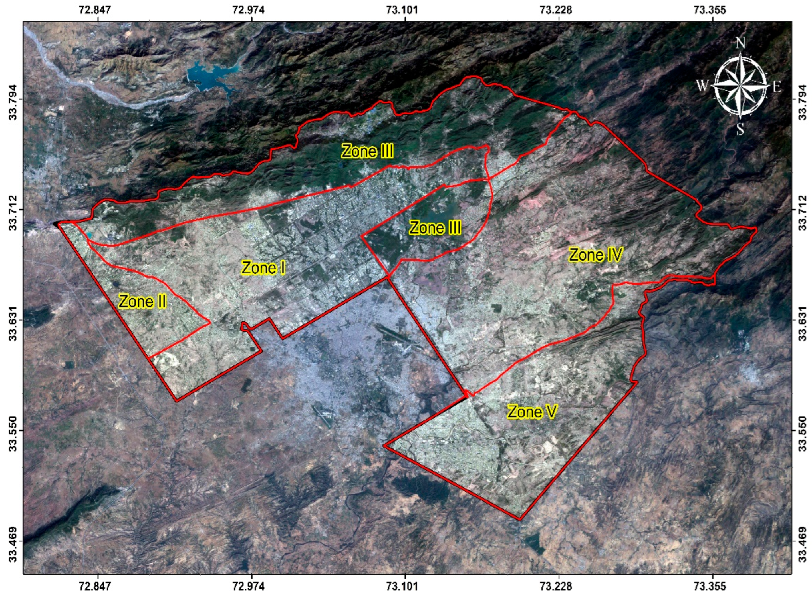
2.1. Study Area

Islamabad, Pakistan’s capital, is geo-located at 33°28′ latitude and 73°22′ longitude. It consists of five zones according to the master plan of ICT (Figure 1). Zones I and II are divided into sectors with approximately 2 km × 2 km for each sector. Primary and secondary roads in urban areas interlace horizontally and vertically, dividing the urban area into several equal-size sectors. Residential, industries, industrial hubs, public and private services, international embassies, colleges, and so on are also included. Zone III mainly comprises green spaces, forests, and mountains. The conserved Margallah Hills national park land is included in this zone, which is designated as an ecological conservation area. Cropping areas and farmland are the major categories of Zone IV and Zone V, but the south side of Zone V, which is close to Rawalpindi City, is mostly made up of industrial areas and public and private housing schemes.

2.2. Data Acquisition

Land cover mapping was performed using Landsat satellite sensor (OLI), Enhanced Thematic Mapper Plus (ETM+), Thematic Mapper (TM), and Multispectral Scanner System (MSS) sensor images that were orthorectified and cloud-free with a 30 m spatial resolution. A single Landsat scene covers the entire ICT area. For urban modeling in Islamabad, multiple datasets have been used. The data used are (1) scanned maps for the delineation of zone boundaries and other important locations of societies; (2) Landsat TM ETM+ OLI images (2000, 2005, 2010, 2015, and 2020) (to classify the LULC); and (3) Global Digital Elevation Model (GDEM) (used to obtain surface elevation for modeling) data, as well as point data including POIs, road network data, and water channel network data obtained from the “Open Street Map (OSM). The datasets were projected using the Universal Transverse Mercator (UTM) coordinate system WGS-84 UTM Zone 43N. Multi-temporal Landsat satellite images were clipped to the Islamabad boundary, and LULC maps were generated for the years 2000, 2005, 2010, 2015, and 2020 using a support vector machine (SVM). Satellite imagery was obtained during the post-monsoon season (October–November) in Islamabad due to the clear skies and minimal cloud cover. During this period, vegetation is stabilized after the monsoon, providing distinct spectral signatures for different land cover classes. The images were classified into four categories: built-up (manmade structures), bareland (exposed soil and construction sites), vegetation (forests, crops, and urban greenery), and water bodies (rivers, lakes, and ponds). The methodology employed in this research is clearly outlined in the schematic diagram (Figure A1, Appendix A), which delineates the sequential steps of the approach.

2.3. Spectral Indices for Sustainability Assessment and Accuracy

To increase the classification accuracy and improve information about land cover, spectral indices were used [26,44]. These candidate features were evaluated using three spectral indices: (1) Normalized Difference Vegetation Index (NDVI), (2) Normalized Difference Built-up Index (NDBI), and (3) Normalized Difference Water Index (NDWI). The indices are classified into two major types: (1) vegetation conditions and (2) soil conditions.

$$NDVI=\left(NIR-R\right)/\left(NIR+R\right)$$

(1)

$$NDBI=\left(SWIR-NIR\right)/\left(SWIR+NIR\right)$$

(2)

$$NDWI=\left(Green-NIR\right)/\left(Green+NIR\right)$$

(3)

2.4. Support Vector Machine

The support vector machine (SVM) is a supervised classification technique, a powerful machine learning algorithm, and a binary classifier used to categorize satellite data. Despite using a limited training dataset, SVM has gained popularity due to its high precision, robustness, and strong performance outcomes. SVM is particularly effective for image classification as it optimizes the separation margin between classes, enhancing its ability to generalize well and resist overfitting, especially in high-dimensional feature spaces. It operates based on the principle of structural risk minimization (SRM), which aims to divide the classes and maximize the margin between them using a decision surface called the optimal hyperplane and a small training set [45]. It operates based on the principle of structure risk minimization (SRM), which divides the classes and increases the margin between them by using a decision surface called optimal hyper-plane and a small training field [46]. The data points closest to the hyperplane are called support vectors [47,48]. Instead of the dimensionality of the evolving space, the number of support vectors in the final classifier expresses its complexity. As a result, when compared to other techniques, SVMs are typically less susceptible to over-fitting issues [43,49].

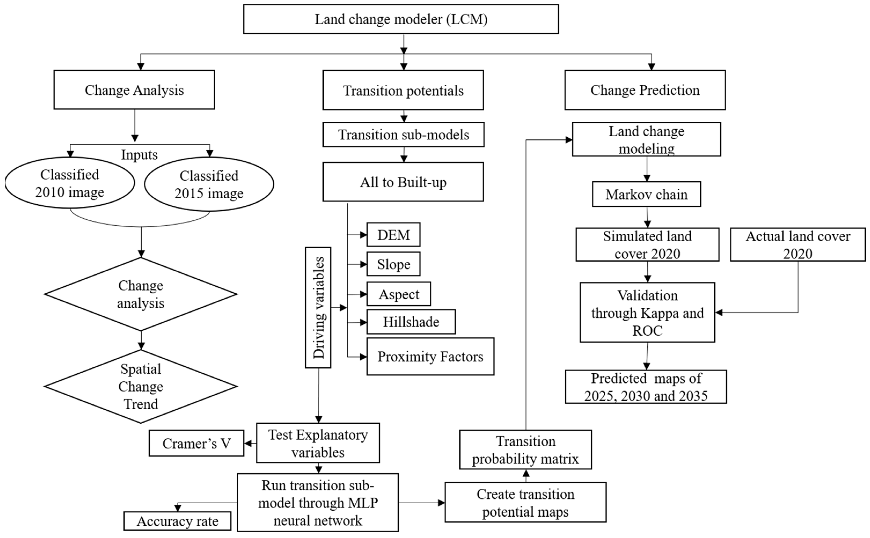
2.5. Transition Potential Modeling and Driving Factor Selection

2.5.1. Transition Potential

Land transitions for the years 2000–2005, 2005–2010, 2010–2015, and 2015–2020 were identified, and then, transition potential maps were generated by approximating the reasonable change in each pixel. The transition potential is generated by using the trained data from a multilayer perceptron (MLP). A value of 0 indicates that there is no transition potential, while a value of 1 indicates the highest transition potential.

2.5.2. Selection of Explanatory Variables

The Cramer’s V values indicate the instructive value of each driver based on a likelihood table analysis before using auxiliary data in the LCM. Cramer’s V does not provide convincing evidence that a specific variable is responsible for land use change as it only indicates the influence of that particular variable towards the change [27,50]. A higher Cramer’s V value indicates a strong influence of that variable, whereas as a low Cramer’s V value indicates rejection of that variable. In our study case, Cramer’s V values are around 0.05; therefore, all the P values are very low [27,51].

$$CV=\sqrt{{\displaystyle \frac{x^2}{\left(N\right)(\min r-1,c-1)}}}$$

(4)

$$x^2=M\left[{{\displaystyle \sum }}_{i=1}^s{{\displaystyle \sum }}_{r=1}^n\left({\displaystyle \frac{q_{ir}^2}{M_i+M+r}}-1\right) \right]$$

(5)

where $x^2$ is the statistical test to determine the dependency of variables, M is the sample number, s is the sample size, n is discrete intervals, $q_{ir}^2$ is the total number of nonstop values, $M_i$ is the total number of objects belonging to i class, and M + r is the total number of nonstop feature values.

2.5.3. Multilayer Perceptron

A multilayer perceptron (MLP) is a feed-forward neural network (NN) that uses back propagation (BP) to forecast results. It is a non-parametric algorithm that does not consider the multi-co-linearity [15,52]. An ANN consists of layers of interconnected nodes (also called neurons) that work together to process and learn patterns from input data. MLP comprises three layers: an (1) input layer, (2) hidden layer (sets of processing nodes), and (3) output layer. Through a network of weighted links that are iteratively changed by the algorithm, it indicates relationships between changes in land use and their explanatory variables. Non-linear relationships are the outcome of data flowing via hidden layers from an input layer to an output layer in one direction. Two types of predictions are generated by the LCM: (1) soft predictions and (2) hard predictions [21,52]. A forecast graphic is obtained from a hard prediction centered on the Multi-Objective Land Allocation (MOLA) module. Each pixel is allocated by this module to a ground cover group that has a higher probability of existence. A soft prediction is a continual mapping of fluctuating susceptibility; it shows the likelihood that a given class pixel will change to a specified land cover class pixel. The transition probability matrix was produced by the Markov chain, which determines how much land is allocated to a theme class [53,54].

2.6. Future LULC Mapping and Change Analysis

Change prediction is the final step, in which the future is predicted using an ANN–Markov chain and transition potential maps along with the history rate of change.

2.6.1. Markov Chain Model

The Markov model has gained widespread recognition as a dependable and trustworthy tool for ecological modeling, tracking, and trend simulation. It may also be used to anticipate future scenarios at various spatial scales [55]. Potential LULC changes are predicted by this model from one cycle (t = 1) to the next (t + 1) (Equations (6)–(8)) based on the transition potential matrix for every LULC class [56,57]. In this approach, the changes are seen as stochastic processes. Conversely, the transition matrix is essential for upcoming LULC simulations [57,58].

$$S\left(t+1\right)=P_{ij}\ast S\left(t\right)$$

(6)

$$P=\left[P_{11}{P}_{12}\cdots \right]P1n⋮\ddots ⋮Pn1 Pn2\cdots Pnn$$

(7)

$$0\le P_{ij}<1 and {{\displaystyle \sum }}_{j=1}^n{P}_{ij}=1, \left(i,j=1,2,\dots .n\right)$$

(8)

where S(t) indicates the state of the system at time t; S (t + 1) indicates the state of the system at a time (t + 1), and P_ij indicates the transition probability matrix from the present state, i, to the next state, j. Using the Markov chain model, several studies have been carried out to evaluate the potential LULC scenario in the future.

2.6.2. Model Validation

Model validation was performed using Kappa statistics and the relative operating characteristic (ROC) curve. Kappa statistics is a quantitative tool for determining the best match or the degree of agreement between observed maps and model forecasts [58].

The relative operating characteristic (ROC) curve illustrates the relationship between the true positive rate (vertical axis) and the false positive rate (horizontal axis), with values ranging from 0 to 1, where 1 indicates a perfect fit and 0.5 represents a random fit. In this study, a threshold value of 100 was utilized to evaluate model performance. ROC analysis was employed in land change prediction modeling to assess the model’s predictive accuracy for a specific land cover class within a multi-class framework [49,59,60,61]. The actual 2020 LULC map was compared with the projected 2020 LULC map. The area beneath the curve (Figure 6) reveals that most of the area remained unchanged, demonstrating that the expected and actual land use situations are relatively similar. After validating the model, prediction maps for 2025, 2030, and 2035 were generated.

2.7. Landscape Metrics

Landscape metrics provide a quantitative link between biological and environmental processes and patterns in the landscape. They provide numerical information about the structure, arrangement, and dimension of the landscape, facilitating long-term comparisons and aiding in the creation of hypothetical futures [15,62,63]. Landscape metrics are crucial instruments for defining spatial dynamics and ascertaining the spatial and temporal arrangement of landscape features [55,64,65].

The metric category ought to mirror the diversity of patterns observed across the landscape; nonetheless, its application needs to be restricted, especially in closely related indices [10,64,66]. Three categories can be used to group them: patch, class, and landscape. The metrics used in this study at the class level are shown in

Table 1. Description of landscape matrices.

Metrics	Metric Name	Acronym Unit	Description
Proximity	Mean Proximity Index (MPI)	m	A measure of a habitat class’s interconnectedness. Within a given search radius, the magnitude and similarity of every area with the same type of habitat are taken into account.
	Mean Euclidean Nearest Neighbor Distance (ENN_MN)	m	The complexity of the shape enhances its shortest edge-to-edge interval between two patches of the same kind. It describes whether a landscape or habitat type is related or isolated.
Diversity and Texture	Contagion (CONTAG)	%	Calculate the overall likelihood that a patch of cells that are adjacent to one another will be of the same type.
	Shannon’s Diversity Index	None	Signify landscape diversity derived from the abundance of patch types.
Shape and Edge	Density of Edges (ED)	m/ha	Calculate the total lengths of all patch-type edge segments that fit the unit area. The complexity of each patch form is demonstrated by the edge density.
	Largest Patch Index (LPI)	%	The proportion of the overall landscape area to the biggest patch of that particular patch kind.
	Area Weighted Mean Fractal Dimension Index (AWMPFD	None	Divide the total patch area by the average dimensions of patches of a specific patch type.
	Mean Shape Index (MSI)	Meter per Square Kilometer (m/km2)	Measures the patch shape’s complexity in comparison to a regular shape of the same dimension. Its worth rises as the form become more complicated.
	Mean-Perimeter-to-Area Ratio (MPAR)	Meter per Square Kilometer (m/km2)	The perimeter-length-to-patch-area ratio determines the patch form complexity. It describes shape complexity without requiring a regular Euclidean shape to be used (square).
Patch size and Density	Patch Density (PD)	Number of patches per 100 ha	The number of patches per unit area
	Percentage of Landscape (PLAND)	%	The combined landscape area.
	Mean Patch Area (MPA)	ha	Each class’s average patch size
	Number of Patches (NP)	%	The cumulative number of patches in a given category’s landscape.
	Mean Patch Size (MPS)	Square Kilometer (km2)	The total area of all patches in the class is divided by the total number of patches in the class

.

3. Results

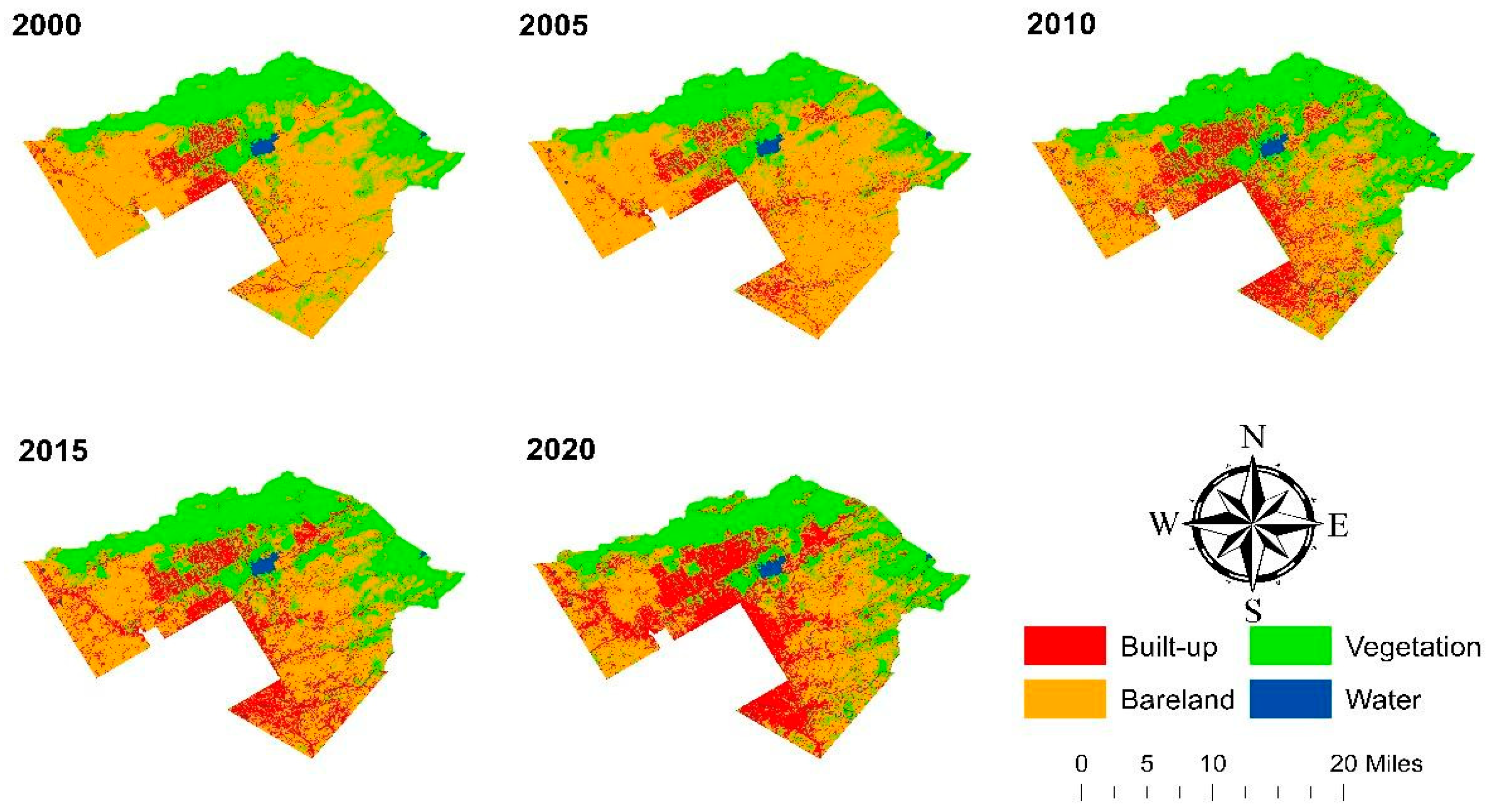
3.1. Spatiotemporal Distribution of LULC Types in Islamabad (2000–2020)

For the study period (2000–2020), spatiotemporal quantitative analysis of each LULC thematic class was conducted in requisites of percentage and total area (see

Table 2. Area statistics of the classified images for the years 2000–2020.

LULC Class	Area (km2)
Years	2000	2005	2010	2015	2020
Built-up	58.09	100.01	166.95	201.33	256.49
Bareland	414.37	404.64	358.67	329.89	326.49
Vegetation	428.28	396.85	373.24	367.88	316.53
Water	11.05	9.71	11.98	11.45	10.76
Total	911.79	911.21	910.84	910.58	910.28

and Figure 2). Each LULC class changed significantly during 2000–2020. The dominant LULC class in Islamabad in 2000 was vegetation (forest, cropland, and grassland), making up more than 46 percent of the entire region, and bareland, which accounted for 45.45 percent of the total area. Water and built-up areas had the lowest percentages of 6.37 percent and 1.21 percent, respectively. However, in 2005, the spatial extent was wide-ranging among land use classes, and the built-up area was higher compared to other classes. In 2010, vegetation and bareland were still the dominant categories, representing 40.98% and 39.37%, respectively, of the total area; with the continuation of the previous period, it showed a declining trend. These trends continued for 2020 with an increase in built-up area (58.09 km² to 256.49 km²) at the cost of loss of vegetation (428.28 km² to 316.53 km²) and bareland (414.37 km² to 329.8 km²). The results show a continual decline in vegetation area and increase in built-up area at an exponential rate over the last two decades.

3.2. LULC Inter-Category Transition in Islamabad (2000–2020)

The estimated land cover area for each year image (2000 to 2020) and their spatial distributions are shown in Table 2. Over the last two decades (2000–2020), the built-up area has increased while vegetation cover has decreased significantly. The major transformations observed during the study period were vegetation, bareland, and built-up area. From 58.09 km² (6.37%) in 2000 to 256.49 km² (28.18%) in 2020, the built-up area increased by 6.37%, whereas vegetation cover decreased significantly from 428.28 km² (46.97%) in 2000 to 316.53 km² (34.77%) and bareland from 414.37 km² (45.45%) to 326.49 km² (35.87%) during the study period (see

Table 3. The change detection matrix of LULC during the different periods (percentage).

2000–2005	Built-Up	Bareland	Vegetation	Water	Total/LSE	L	G	Change 2000–2005 (km2)	% of Change	Annual Rate of Change (%)
Built-up	58.08	0.00	0.00	0.00	58.08	0.00	41.78	41.92	72.15	10.86
Bareland	32.04	379.48	0.00	1.85	413.37	33.89	24.60	−9.72	−2.34	−0.47
Vegetation	8.84	21.81	396.73	0.53	427.91	31.18	0.00	−31.43	−7.33	−1.52
Water	0.91	2.78	0.00	7.32	11.01	3.69	2.38	−1.35	−12.18	−2.59
Total/PSL	99.86	404.08	396.73	9.70	910.37	68.76	68.76	−0.58	50.28
2005–2010
Built-up	99.98	0.00	0.00	0.00	99.98	0.00	66.76	66.94	66.93	10.24
Bareland	57.48	343.87	0.00	2.58	403.93	60.06	14.18	−45.97	−11.36	−2.41
Vegetation	8.41	13.80	373.13	0.90	396.24	23.11	0	−23.60	−5.94	−1.22
Water	0.87	0.38	0.00	8.45	9.70	1.25	3.47	2.27	23.40	4.20
Total/PSL	166.74	358.05	373.13	11.93	910.37	84.42	84.42	−0.37	73.04
2010–2015
Built-up	166.90	0.00	0.00	0.00	166.90	0.00	34.32	34.38	20.59	3.74
Bareland	23.78	285.73	47.59	0.98	358.08	72.35	43.60	−28.77	−8.02	−1.67
Vegetation	9.95	42.70	318.34	1.31	372.31	53.97	48.87	−5.35	−1.43	−0.28
Water	0.59	0.89	1.28	9.16	11.93	2.76	2.29	−0.52	−4.34	−0.88
Total/PSL	201.23	329.33	367.22	11.45	910.37	129.08	129.08	−0.26	6.80
2015–2020
Built-up	201.28	0.00	0.00	0.00	201.28	0.00	55.81	55.15	27.39	4.84
Bareland	32.48	269.36	27.39	0.50	329.73	60.36	56.92	−3.40	−1.03	−0.20
Vegetation	22.62	56.40	287.69	0.60	367.31	79.62	28.70	−51.35	−13.95	−3.00
Water	0.72	0.51	1.31	8.91	11.45	2.54	1.10	−0.69	−6.06	−1.25
Total/PSL	257.09	326.28	316.38	10.01	910.37	142.53	142.53	−0.30	6.34
2000–2020
Built-up	58.08	0.00	0.00	0.00	58.08	0.00	198.7	198.39	341.51	0.30
Bareland	130.89	250.40	30.56	1.58	413.44	163.04	75.65	−87.87	−21.20	0.21
Vegetation	64.79	75.14	285.28	1.47	426.67	141.39	31.08	−111.74	−26.09	0.21
Water	3.02	0.51	0.52	6.96	11.00	4.05	3.05	−0.289	−2.62	0.22
Total/PSL	256.77	326.05	316.36	10.01	910.37	308.48	308.4	−1.51	291.59

), respectively. In 2000, Islamabad majorly comprised vegetation cover, covering 428.28 km², which is 46.97% of the total geographical area, whereas bareland was the second major class, covering 414.37 km² (45.45%). The water class is relatively stable during the study period. The fluctuation in water class is due to seasonal flow, which is dependent on weather conditions. However, the overall water class decreased from 11.05 km² (1.21%) to 10.76 km² (1.18%) during 2000–2020.

The change analysis results for the periods 2000–2005, 2005–2010, 2010–2015, 2015–2020, and 2000–2020 (Table 3) show a notable decrease in the amount of vegetation cover and bareland, with a trend of built-up area growth. Table 3 shows that during 2000–2005, vegetation cover decreased by approximately 31.43 km² (7.34%) with a 1.52% annual rate of change. Bareland decreased by 9.72 km² (2.35%), and built-up area increased by 41.92 km² (72.15%). The period 2005–2010 showed the same significant changes as in 2000–2005. In this period, vegetation cover shows a decreasing trend of approximately 23.61 km² (5.95%) with a 1.23% annual rate of change. Bareland decreased considerably by 45.97 km² (11.36%), built-up area increased by 66.94 km² (66.94%) with a 10.25% annual rate of change, and water cover increased by 2.27 km² (23.41%). The period 2010–2015 was a period of higher variation in land use. During this period, bareland decreased by 28.77 km² (8.02%), the built-up area increased by 34.39 km² (20.60%) with a 3.75% annual growth rate, and vegetation cover decreased by 5.36 km² (1.43%). During 2015–2020, vegetation cover decreased by approximately 51.35 km² (13.96%) with a 3.01% annual rate of change. The bareland area decreased by 3.40 km² (1.03%), and the built-up area increased by 55.15 km² (27.39%) with a 4.84% annual rate of change. Comparing the land use statistics for the year 2020 with the results of our baseline study in the year 2000 revealed that the alarming rate of city growth is accompanied by an increase in the built-up area by 341.51% and a decrease in vegetation cover by 21.21% during this period. LULC changes from 2000 to 2020 show a land transition of classes from bareland and vegetation cover to urban area, which increased more towards the southern side of the study area. The multiple contributory elements are responsible for the expansion of urban sprawl in the Islamabad district. These include a higher annual population growth rate, user preferences (those in the upper class go to low-density residential regions because they want to live in villas or bungalows which cannot be constructed in congested city districts), low property taxes, a lack of urban planning, the need for additional living space, physical topography, inexpensive land prices, increasing living standards, and high monthly incomes 50.

3.3. Accuracy Assessment for the Years 2000–2020

To assess the accuracy of land cover maps derived from satellite images, a stratified random sampling method was employed to represent various land cover types within the study area. Accuracy was evaluated by using 100 points, which were based on ground truth data and visual interpretation. The classification results were compared with the reference data through statistical analysis using error matrices. Additionally, a non-parametric Kappa test was conducted to further measure classification accuracy, as it takes into account not only the diagonal elements but also all elements within the confusion matrix. The overall accuracy for the years 2000–2020 is presented in

Table 4. Accuracy assessment metrics for classified land use–land cover images (2000–2020).

Years	User Accuracy (%)				Producer Accuracy (%)				Overall Accuracy	Kappa Coefficient
	Built-Up	Bareland	Vegetation	Water	Built-Up	Bareland	Vegetation	Water
2000	92.00	93.33	89.74	83.33	95.83	87.50	92.11	83.33	91.00	0.8700
2005	95.65	93.10	89.74	88.89	91.67	93.10	92.11	88.89	92.00	0.8864
2010	96.43	88.00	89.74	100.00	90.00	84.62	97.22	100.00	92.03	0.8864
2015	93.33	89.66	94.44	100.00	93.33	89.66	97.14	83.33	93.00	0.8996
2020	93.75	89.66	96.67	88.89	90.91	96.30	90.63	100.00	93.00	0.9018

.

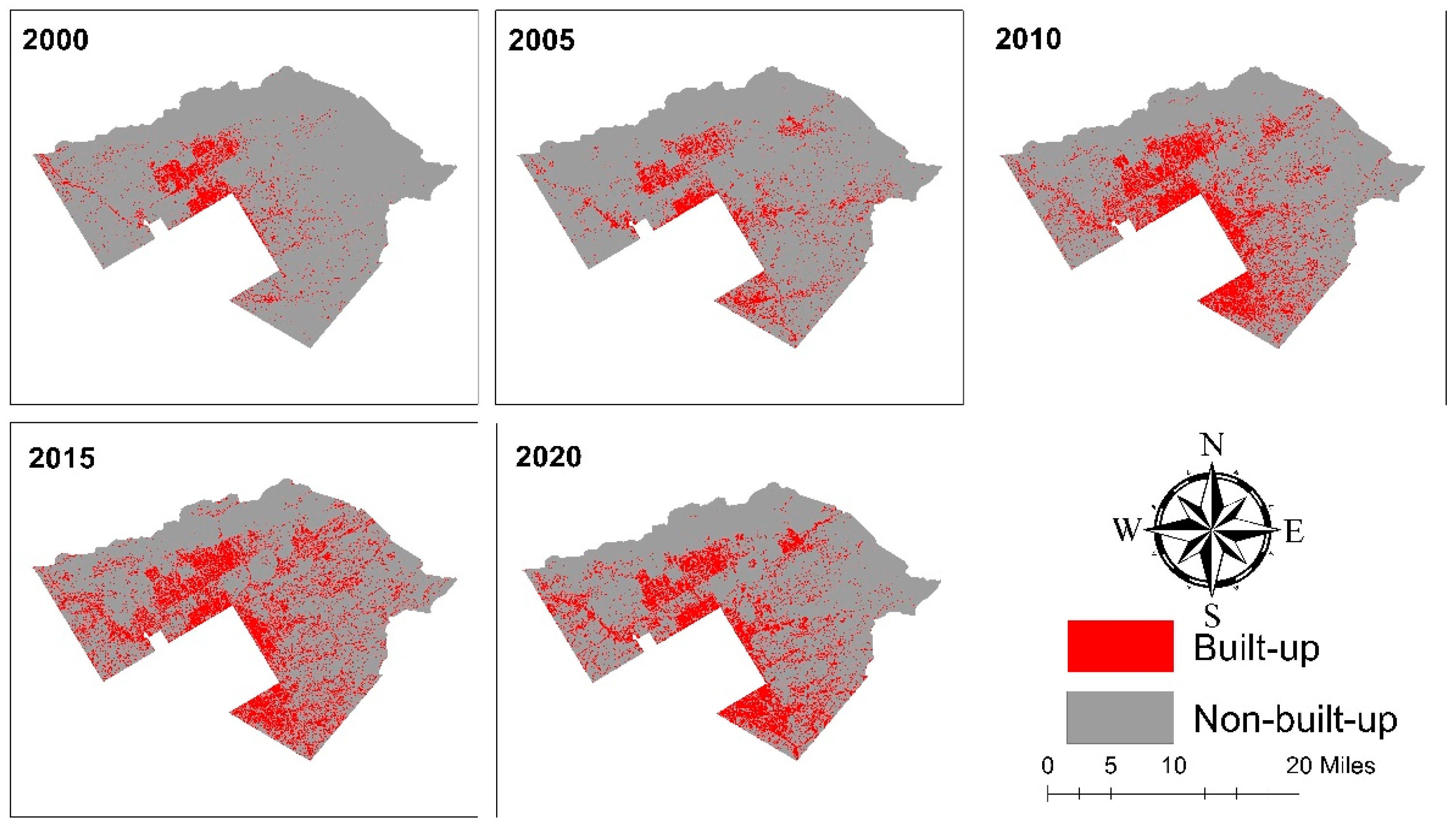
3.4. Land Cover Changes in Built-Up and Non-Built-Up Areas (2000–2020)

The increase in Islamabad’s infrastructure over the past 20 years has been a major factor in the city’s urbanization, exhibiting the absence of suitable planning. The purpose of this study was to ascertain and explore the geographical boundaries of inhabited regions throughout the study period. Figure 3 and

Table 5. Built-up and non-built-up areas in Islamabad (2000–2020).

Years	2000		2005		2010		2015		2020
LULC Class	Area (km2)	% of Total	Area (km2)	% of Total	Area (km2)	% of Total	Area (km2)	% of Total	Area (km2)	% of Total
Built-up	58.09	6.37	100.01	10.98	166.95	18.33	201.34	22.11	256.49	28.18
Non-Built-up	853.7	93.63	811.2	89.02	743.89	81.67	709.24	78.53	653.78	71.82
Total	910.00	6.37	910.00	10.98	910.00	18.33	910.00	100.00	910.00	28.18

show both land use and land cover maps of built-up and non-built-up areas.

As seen in Table 5, the built-up area in 2000 was 6.37%, which increased to 10.98% in 2005, 18.33% in 2010, 22.11% in 2015, and 28.18% in 2020, respectively. The horizontal expansion and transfer of land cover classes contributed to the increase in built-up territory (vegetation and bareland into built-up area). Overall, 22% of the land was transferred from other classes to the built-up class (Figure 3), which is a concerning condition for the city and urban planners.

3.5. Persistence and Vulnerability of LULC Class Dynamics in Islamabad

The gain-to-persistence ratio (G/P) shows the likelihood of gaining relative to persistence in all LULC groups. The net-change-to-persistence ratio (N/P) measures how much the LULC class has gained or lost in comparison to its persistence [61]. The loss-to-persistence ratio determines how vulnerable a ground cover is to transformation. The LULC has a higher chance of gain than persistence if the gain-to-persistence ratio (G/P) is greater than 1. If the loss-to-persistence ratio (L/P) is greater than 1, the LULC is more susceptible to changes in other LULC classes than to persistence [61]. However, for the built-up class, all LULC groups’ L/P and G/P values are less than 1, indicating that the pattern reflects a loss rather than a gain (

Table 6. Loss-to-persistent (L/P), gain-to-persistent (G/P), and net-change-to-persistent (N/P) ratios of LULC classes in Islamabad (2000–2020).

	L	Tc	Nc	ANC	S	G	P	G/P	L/P	N/P
Built-up	0.00	198.70	−198.70	198.70	0.00	198.70	58.08	3.421	0.000	3.421
Bareland	163.04	238.68	87.39	87.39	151.30	75.65	250.40	0.302	0.651	0.349
Vegetation	141.39	172.47	110.31	110.31	62.16	31.08	285.28	0.109	0.496	0.387
Water	4.05	7.10	1.00	1.00	6.10	3.05	6.96	0.439	0.582	0.143

). The built-up class has a G/P of 3.421, showing that the gain is important as opposed to persistence. As a result, Islamabad could be particularly vulnerable to the loss of vegetation cover. The G/P of vegetation is 0.109, meaning that vegetation gain is negligible in comparison to its persistence from 2000 to 2020. The values for bareland and water are 0.302 and 0.439, respectively, showing less gain than loss. Similarly, the L/P ratio of the built-up class is negative, indicating a lower susceptibility to failure than to persistence, implying that there is no loss in the built-up class. Bareland and vegetation, on the other hand, have a greater risk of losing to other LULC classes with values of 0.651 and 0.496, respectively; bareland and vegetation reflect a higher susceptibility to loss than persistence. Water, with a value of 0.582 below 1.0, has a reduced likelihood of transitioning to other land uses (Table 6).

The net-change-to-persistence ratio (N/P) for the built-up class is 3.421, meaning that its net gain is greater than its loss with a net change of −198.70. Water has a value of 0.143, indicating a lower propensity to change. Over the study period, bareland and vegetation all experienced net losses of around 0.349 and 0.387, respectively, indicating improvements in these LULC groups compared to others.

3.6. Future Simulation

By using the LCM, projections are made for the years 2025, 2030, and 2035. The LCM produces two different kinds of forecasts: hard forecasts and soft forecasts. A forecast is obtained through a hard prediction that is centered around the MOLA module [53,54]. Each pixel in this module corresponds to a different land cover class, which has a higher chance of being changed. It indicates the probability that a pixel will be converted to a different class of land cover. Lastly, throughout a cycle of N years and T2–T1, the transition likelihood matrix derived from the Markov chain determines how much each land use is allocated to a thematic class [12].

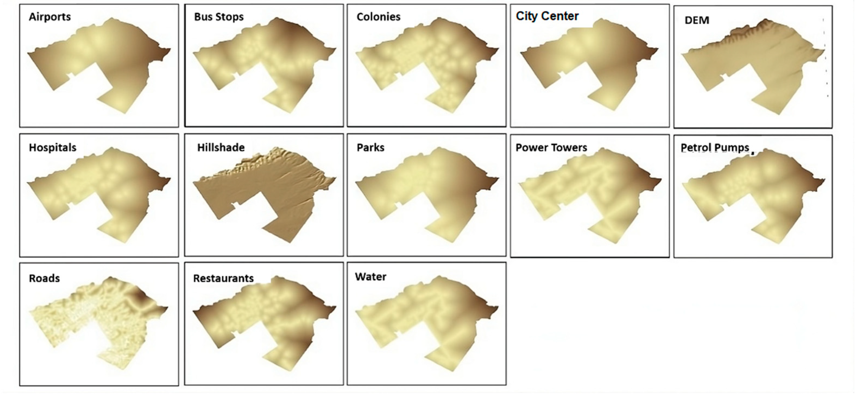
Selection of Driving Variables for Transition Potential Modeling

The most crucial stage in modeling growth is connected to the LULC transition associated with the driving factors [29,30,31]. The model produces reasonably accurate findings. Since each location is unique and the factors causing change are not always common, no uniform set has been developed, although multiple variables responsible for LULC change have been identified and utilized by the researchers to forecast the change [29]. Land transitions also vary from case to case, and the degree to which the driving factors contribute to the transitions also differs. Urban growth prediction modeling involves the computation of Cramer’s V, which identifies the best driving variable for modeling urban growth and measures the association strength between each pair of variables used in modeling [47].

Cramer’s V, which calculates the ideal driving variable for modeling urban development and assesses the degree of association between each set of variables used in modeling, is computed as part of the LULC simulation modeling process. Selected Cramer’s V values are given in

Table 7. The quantified relationship between chosen driving factors and the LULC classes is described by Cramer’s V coefficients.

Driving Factor	Cramer’s V
Colonies	0.2924
DEM	0.2684
Airports	0.2647
Bus Stops	0.2628
Hospitals	0.2432
Roads	0.2202
Water Courses	0.2168
Restaurants	0.2125
Hillshade	0.2074
Parks	0.2039
Power Towers	0.2032
City Centers	0.1932
Petrol Pumps	0.1794

and Figure 4, which show the quantitative rank of correlation between 13 driving factors and 4 significant land use categories.

The highest Cramer’s V for restaurants, 0.2924, was found for colonies, which means that the sturdiest driving force in the case of urban growth prediction of Islamabad was the establishment of new housing colonies and societies. The second most important factor for our study was the DEM, which depicts Islamabad being a hilly area, with the availability of relatively plain areas driving urban expansion. Other driving forces as ranked by the value of Cramer’s V include airports, bus stops, hospitals, roads, restaurants, parks, and power towers, with the distance to petrol pumps having a value of 0.1794, which is only somewhat linked to a few categories of land and therefore shows the lowest inclusive degree of connectivity. The Cramer’s V value for city centers, 0.1932, has also been well associated with the distance to built-up areas and roads, where main roads are all still outlying.

3.7. Model Validation Results

Figure 5 presents maps of land cover and use for 2020, including both real and predicted data, along with their area statistics (see

Table 8. Land cover map of 2020 with current and estimated land use statistics.

Classes	Area (km2)
	Actual	Predicted
Built-up	256.49	232.90
Bareland	326.49	307.51
Vegetation	316.53	358.73
Water	10.76	10.89
Total	910.28	910.03

). According to tabular details and visual analysis of simulation modeling findings, the projected thematic map for 2020 closely resembles the real theme map for that year. Model validation is essential for applying MLPNN in urban growth prediction studies, with Kappa statistics and relative operating characteristics being utilized for this purpose. A more detailed analysis was conducted using Kappa statistics and relative operating characteristics (ROCs). The Kappa statistics, which compared the projected 2020 LULC map with the actual 2020 LULC map, yielded the following results: Kappa = 0.94, Kno = 0.95, Kappa location = 0.99, and Kappa standard = 0.96. Meanwhile, the ROC value, represented by the area under the curve, was 0.914. Relative operating characteristics (ROCs) in land change prediction modeling are used to infer the accuracy predicted by the model of one class out of various other types of land cover and land usage [49]. A comparison was made between the expected and actual 2020 LULC maps, and verification was achieved using the ROC curve. The region under the curve (Figure 6) shows that the bulk of the survey area experienced no change, showing that the predicted results and the actual land use situation are very consistent. After validating the model, 2025, 2030, and 2035 prediction maps were generated.

The relative operative characteristic (ROC) curve is used to examine the relationship between actual and expected land use–land cover charts. The greater the number of ROC values that outweigh the upper left corner, the more accurate the model is. The reliability between the real and forecast land use–land cover chart is represented by the ROC value for this model.

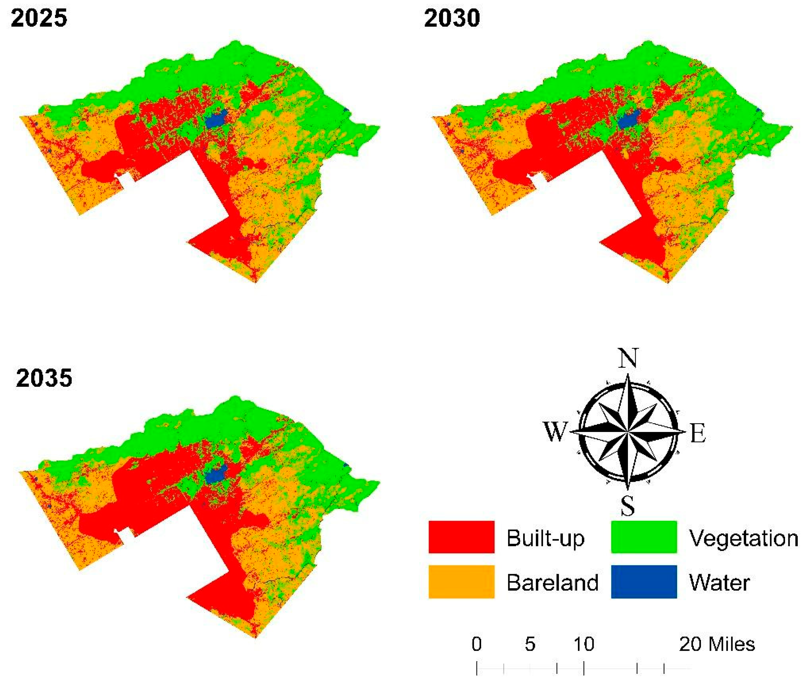
3.8. Future Simulation/Scenario

Simulated maps pertaining to the years 2025, 2030, and 2035 are shown in Figure 7. Landscape statistical change analysis of simulated LULC classes can be observed in

Table 9. LULC area statistics and change analysis.

LULC	Area (km2)				Change Rate (%)
Years	2020	2025	2030	2035	2020–2025	2020–2030	2020–2035	2000–2035
Built-up	256.49	263.34	293.47	319.57	2.67	14.42	24.59	45.10
Bareland	326.49	290.11	272.56	258.09	−11.14	−16.51	−20.94	−37.71
Vegetation	316.53	346.19	334.10	322.93	−9.37	−5.55	−2.02	−24.59
Water	10.76	10.36	9.87	9.41	−3.73	−8.30	−12.56	−14.85

. The result of change detection from 2020 to 2035 shows that the built-up area will increase from 256.49 km² in 2020 to 319.58 km² in 2035, while vegetation cover will increase from 316.53 km² in 2020 to 346.20 km² and then decrease to 322.94 km² in 2035 with a −0.71 yearly growth rate. However, the water class will remain persistent. In the built-up class, the average change in land use–land cover from 2000 to 2035 is predicted to be 261.49 km² (Figure 8).

The expansion of the urbanized region of Islamabad varies over time, i.e., 2.67% during 2020–2025, 14.42% during 2020–2030, 24.60% during 2020–2035, and 450.11% during 2000–2035, as shown in Table 9. A significant increase in the built-up class has been associated with a decrease in bareland and vegetation cover. The bareland declined by −11.14% during 2020–2025, having a yearly rate of growth of −2.36%, and is predicted to decline by −1.57%, with a yearly rate of change of −20.95, in 2020–2035 (

Table 10. Annual rate of change.

Annual Rate of Change (%)				Change in Area (km2)
2020–2025	2025–2030	2030–2035	2020–2035	2020–2025	2020–2030	2020–2035
0.53	2.17	1.70	7.47	6.85	36.98	63.08
−2.36	−1.25	−1.09	−1.57	−36.37	−53.92	−68.39
1.79	−0.71	−0.68	0.13	29.66	17.57	6.40
−0.76	−0.97	−0.95	−0.90	−0.40	−0.89	−1.35

). Because of economic policy, employment, manufacturing, and infrastructure growth, simulation results show that such developments will persist in the future. These modifications have negative consequences for the green urban environment.

Future Simulation Gain, Loss, and Net Change

The loss, gain, and net contribution in LULC from 2020 to 2035 are presented in

Table 11. Total gain, loss, and net contribution from 2020 to 2035.

Classes	Gain	Loss	Net Contribution
			Built-Up	Bareland	Vegetation	Water
Built-up	112.51	0.00	0.00	−77.06	−33.81	−1.65
Bareland	25.63	−123.78	77.06	0.00	21.35	−0.26
Vegetation	47.12	−60.05	33.81	−21.35	0.00	0.48
Water	1.54	−2.97	1.65	0.26	−0.48	0.00

and Figure 8. Increases in other LULC groups, mostly the built-up class, would negatively impact the vegetation class. In the upcoming decades, unprecedented urbanization, demographic growth, and social transformation will result in a substantial rise in the built-up class. Table 11 also reveals how each land use–land cover class contributed to a net change in 2020–2035, both positively and negatively. It is worth recalling that the majority of vegetation degradation occurred alongside growth in the built-up and bareland classes. The built-up area in the period 2020–2035 is predicted to gain 112.51 km² at the cost of loss of vegetation and bareland. Vegetation loss was 47.12 km² with a net change of approximately 33.81 km². Water underwent a loss of 2.97 km² and gain of 1.54 km², while bareland experienced a loss of 123.78 km² and gain of 25.63 due to the development of new housing societies (Table 11 and Figure 8).

3.9. Landscape Metrics Analysis

During the study period (2000–2035), landscape measurements were used to define and measure changes in the form, function, and diversity of the landscape. Patch density (PD), AREA MN, ENN MN, Interspersion Juxtaposition Index (IJI), percentage landscape (PLAND), and CONTAG were used to measure the systemic change in thematic classes at the class level. The structure was measured at the landscape level (LL) using measurements such as patch density and scale, form, and isolation or proximity. These include patch density (PD), the mean radius of gyration (MRG), the Largest Patch Index (LPI), the mean area (AREA MN), the mean Euclidean nearest neighbor radius (MED), and the mean-perimeter-to-area ratio (MPAR). The Interspersion and Juxtaposition Index (IJI) and Shannon’s Diversity Index were used to measure the landscape’s diversity (SHDI).

3.9.1. Change in Spatial Composition of the Landscape (Landscape Level)

The Euclidean Nearest Neighbor Distance (ENN MN) and Patch Cohesion Index (COHESION) also indicate a substantial decrease in class connectivity. The built-up class shows the most noticeable change among the land cover classes. In 2000, built-up class patches were scattered, and with time due to population and urban growth, NP for the built-up class increased. From 2000 to 2020 (Figure 9), PD also increased from 12.8704 to 25.0352, representing landscape fragmentation. During the study period, IJI increased when AREA MN decreased, indicating that the sample area is fragmented. During the research period, Shannon’s Diversity Index (SHDI), which describes fragmentation, increased from 0.9423 to 1.1428, while GYRATE MN declined from 36.7885 to 33.4382. As a result, in 2020, the landscape was characterized by heterogeneous land use types, as opposed to a more homogeneous distribution of land use types in 2000. This indicates that the region was more fragmented in 2020 than it was in 2000. This demonstrates that during the study period, some land use divisions dominated the landscape. However, from 2000 to 2020, LPI decreased from 35.927 to 16.8169, indicating landscape fragmentation. The landscape parameters SHDI and IJI, which reflect variety and texture in the landscape, have a hump-backed curve. This suggests that as the ecosystem has become increasingly heterogeneous, disproportional, and complex, the density and internal connectivity of vegetation patches have decreased, and then increased.

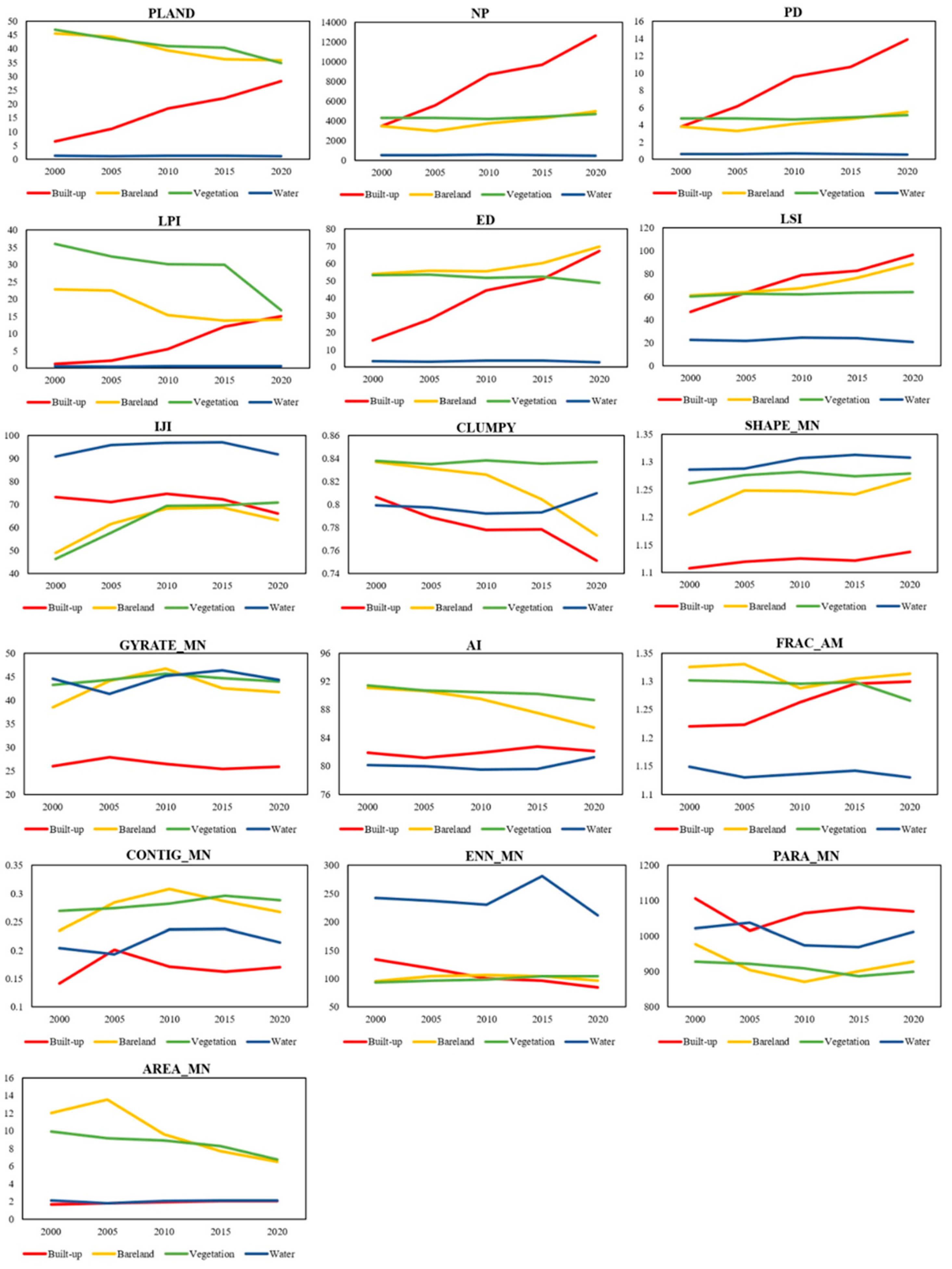
3.9.2. Change in Spatial Composition of the Landscape (Class Level)

Figure 2 illustrates how the patch areas have changed over the last two decades. Between 2000 and 2020, the PLAND of the built-up area grew from 6.3714 in 2000 to 10.9755 in 2005, then to 18.3296 in 2010 and 28.2598 in 2020. The increase in LSI (from 46.7878 to 96.2393), LPI (from 1.2417 to 15.0807), and ED all support this fragmentation trend (from 15.497 to 67.114). The regularity of patterns can be seen in Figure 10. During 2000–2020, the number of patches (NP) in the study area increased (from 3453 to 12,639), as did the mean shape area (SHAPE MN), reflecting a transition toward a larger-grained landscape in the built-up class. IJI in the Islamabad area declined as a result of haphazard economic development and exponential population growth (from 73.3169 to 66.1303), and the mean patch area (AREA MN) increased (from 1.682 to 2.0348) from 2000 to 2020. The LPI for vegetation cover dropped from 35.9627 in 2000 to 35.4018 in 2005 and decreased to 30.092 in 2010 and 16.8169 in 2020, indicating an increased landscape fragmentation of vegetation. From 2000 to 2020, FRAC_AM and PLAND of vegetation cover decreased from 1.3019 to 1.2658 and 46.9708 to 34.7729, respectively. Forest and green spaces decreased from 428.28 km² in 2000 to 316.5309 km² in 2020 due to deviation from the ICT master plan and the development of new housing societies. ENN_MN of forest cover increased from 93.6286 in 2000 to 104.2962 in 2020. This indicates that, as a result of high industrialization and unprecedented population growth, the distance between neighbors is widening over time, implying diversity. The increase in CONTIG MN (from 0.2694 to 0.2878) and IJI confirms this fragmentation trend (from 46.4442 to 70.768). As a result, vegetation fragmentation in the landscape has continued to increase, contaminating the overall biodiversity. The PLAND of bareland decreases from 45.4453 to 35.8673 during the study period. The increase in NP (from 3452 to 5000) and ED (from 53.8839 to 69.6622) and decrease in LPI both support this fragmentation trend (from 22.8523 to 14.0899). From 2010 to 2020, there was steady growth in bareland fragmentation. Furthermore, the increase in the LPI of bareland from 61.2614 to 88.5577 indicated high landscape fragmentation. For the water class, the LSI decreased from 22.7568 to 20.6351.

The rural regions will continue to degrade if land development continues to stretch beyond the city’s limits. Policymakers will need to carefully manage and oversee urban expansion, with an emphasis on preserving dispersed vegetative cover and farmland.

4. Discussion

The majority of quantitative observations are obtained from land survey data, census data, and socio-economic metrics, with a combination of GIS and remote sensing data, such as LULC area statistics and spatial patterns. The effects and patterns of urban growth will be discussed in this section. This study acknowledges challenges such as spatial resolution limitations and data inconsistencies in socio-economic metrics affecting LULC classification accuracy. Additionally, dynamic socio-economic factors introduce uncertainty in urban growth modeling. Future work can benefit from integrating higher-resolution satellite imagery, systematic ground-truth validation, and advanced machine-learning models to improve prediction accuracy and address data limitations.

4.1. Urbanization and Growth Patterns

Leapfrog growth, fringe extension, and internal filling are all typical trends in urban development [67]. In Islamabad, there are four types of urban development patterns: (1) planning extension, (2) village sprawl and leapfrog, (3) combination, and (4) fringe sprawl and infilling. The first form of urban growth trend is described as urban expansion guided by the Islamabad master plan, which was proposed in 1961. For a given time frame, the optimal use of urban land and appropriate zoning for the layout of urban space are determined by the city government’s master plan. To accelerate this pattern, the major highway and road network was first constructed. Then, within the functional zoning districts, industrial, residential, and other complexes are built sequentially, with a focus on Zones I and II, which are designated as urban areas.

The second type of development led to the formation of villages that spread outwards, eventually leading to the formation of a settlement. Sprawl refers to the haphazard creation of low-density settlement areas as a result of unplanned settlement expansion. It is an inexorable cycle of urbanization that occurs against the backdrop of active economic and social growth. Unplanned population expansion results in a leapfrog period of urban development, in which a village located far from the city expands and elevates into a city. In Zone I, this is a normal phenomenon. The third trend is a merger of neighboring towns or villages, which occurs as cities or villages get closer to one another as a result of urban sprawl. Increasing towns or cities to the nearby towns and villages on the periphery, or combining two nearby towns or cities of different sizes into one, are typical examples of this kind of pattern. Zone V is where the typical instances are located. The fourth trend in urbanization and urban expansion includes infilling within Islamabad City and sprawl from the urban periphery. Fringe sprawl is the conversion of classes of LULC varieties to houses and roads on the fringe of cities. The higher housing density is associated with the conversion of non-urban to urban land uses and is also known as infilling inner sprawl. In the middle of Islamabad and north of Rawalpindi city, this trend can be seen in Zones I, II, and IV.

4.2. Urban Growth Factors

Industrial and real-estate production, job demand, master plan, transportation networks, modernity, better services, population, and neighbor urban impact are the major factors driving urban growth in Islamabad. In the study area, industrial and real estate growth is catalyzing economic development. To improve the country’s economic growth, the Pakistani government declared industrial subsidies in 1988. Unplanned population growth results in a leapfrog period of urbanization. The real estate industry is bolstered by the Model Town Humak and the Defense Housing Authority (DHA), which have established many real estate ventures and encouraged economic development in Zone V. Job prospects and wages in rural areas remain inadequate, contributing to significant disparities between urban and rural communities in terms of income and facility levels. As a result, the job market and the expansion of work openings are important aspects of urban planning. The ICT master plan is another aspect that promotes long-term preparation.

The master plan directed the development of Zones I and II. Zone III was relatively undeveloped until it was classified as an ecologically protected area in line with the master plan of Margalla Hills National Park. The bulk of transportation infrastructure is made up of railway and road networks, which play a vital role in developing cities. The road and rail systems in Zones I, II, and IV and the southern part of Zone V are more developed than those in Zone III, allowing for more expansion. The majority of the expansion is concentrated along highways N5 and E2, which run from Bhara Kahu to Farash Town, Chatha Bukhtawar, Alipur, and Ghouri Town, as shown in Figure 11. Zones IV and V have faced extensive expansion. The railway line runs through H-9 and I-9, making it easier for people to travel into and out of the city for work. Rawat is on the mainline that connects Pakistan’s major cities and transports large amounts of freight and raw materials. Modernity and better infrastructure are both driving forces in the urbanization of rural areas.

Islamabad, the Capital Territory, has seen the fastest population growth rate of 4.91 percent in recent decades as a result of numerous ongoing construction activities. From 0.81 million in 1998 to 2.0 million in 2017, the population has grown significantly [12]. Rapid urbanization has put a strain on the region, particularly with a large influx of people fleeing terrorism-affected areas in Pakistan’s north. As a result, we can conclude that Islamabad’s population boom is driving haphazard urban development. The influence of surrounding cities is the most important aspect that synergizes urban sprawl. From the southeast and southwest, Rawalpindi city encircles Islamabad. Along Highway N5 and E2 from Rawalpindi’s boundary, urban sprawl was evident in Zones I, II, IV, and V. A swath of municipalities in Zone IV spreads out from Rawalpindi’s eastern suburbs. Bani Galla, Burma Town, Ali Pur, Chatha Bukhtawar, Shehzad Town, and University Town are located on Islamabad’s eastern side along the E2 highway.

4.3. Socio-Economic Sustainability

Islamabad is far from the ICT master plan due to its poor economic strength and unequal urban development. According to the master plan, economic planning was prioritized in Zones I and II, which are located in the western part of Islamabad, while the majority of the zones were ignored. There is still a lot of land to build on in Zones I and II. Slum sprawl has hampered haphazard population expansion and the development of many other housing communities. The key constraints to cities’ long-term growth are unemployment and poverty. In Islamabad, the majority of population growth and construction was accompanied by slum expansion. Many slum areas, such as Christian Colony, Musharraf Colony, and French Colony, emerged in the early 1960s in the middle of Zone 1; slums also emerged alongside seasonal drain paths in G-7, G-8, F-6, and F-7. Zone V has no contingency area for slums due to industrial development, real estate, and economic growth, while all other areas have experienced the constant emergence of new slums. Slums emerged in Sectors F-6, F-7, F-11, G-7, G-8, H-13, and I-13 and in Zone I; in Jhangi Syedan, Tarnol, and Katan in Zone II; in Shah Allah Ditta, Shah Allah Ditta caves, and Saidpur in Zone III; in Tarlai Kalan, Sohan, Malpur, Ali Pur, Frash City, Kirpa, and Lakh in Zone IV; and in Tarlai Kalan. By the year 2000, new slums had appeared in Zones G-8, -12, and -14, Sector I, and Dhokpracha in Zone II; in Bukhtawar, Kothathyal, Jillani Town, Kuri, Nogazi, Burma Town, and BharaKaho in Zones III and IV; along Highway E-75; and in Bukhtawar, Kothathyal, Jillani Town, Kuri, Nogazi, Burma Town, and Bhara Kaho in Zone Chatta IV.

Another notable urban development in Zone V is Model Town Humak (MTH). Surrounding countries are unstable due to war with a chronic lack of economic prosperity. In Islamabad, there has been a wave of refugees. The Pakistan–Afghanistan border is about 230 km away from Islamabad. A series of military operations along the border, especially in Afghanistan, caused a large number of people and their families to enter Islamabad and other Pakistani cities in 2002. Consequently, the size of Islamabad’s slums has grown to accommodate the needs of displaced residents. New slums have appeared in Zone IV since 2018, including Morian, Pona Faqiran, Mochi, and Mohran. Previous slum areas were not filled due to the war on terror, and refugees flooded these and other areas, contributing to Islamabad’s unequal economic growth.

5. Conclusions

Over the past 20 years, Islamabad’s LULC has changed significantly as a result of induced socio-economic activity. For long-term urban planning, providing knowledge on urban development and historical tendencies in urban growth is essential. The back propagation technique of the Multilayer Perceptron Neural Network was used to calculate urban growth for the years 2000–2020 and predicted for the years 2020, 2025, 2030, and 2035 in the study area. According to the study, the non-built-up surface area has declined by 93.63% in the last two decades, from 853.7 km² in 2000 to 653.788 km² in 2020. Meanwhile, between 2000 and 2020, the built-up area has increased from 6.37% to 28.18%. Vegetation cover and bareland are the major sources of development. According to the report, the metropolitan area grew by 341.51% from 58.09 km² in 2000 to 256.49 km² in 2020. Urban prediction modeling revealed further expansion trends, which show that there will be a huge increase of 450.11% in the urban area until the year 2035 compared to the year 2000, with a decrease of 24.60% in vegetation area and 37.71% in bareland. Village sprawl, proposed extension, fringe sprawl, and mixing are the four urban development phenomena identified by the spatial growth trends. In Islamabad, there are eight factors behind urbanization: industrial and real estate growth, job environment, master plan, transit infrastructure, modernity, better facilities, population, and neighbor urban impact are all topics that need to be addressed. Despite economic growth on almost all sides of the city, spatial patterns indicate that the south of Islamabad (Zone V) has undergone unchecked development, focused on urban growth and industrial development.

In Zones I and II, the master plan largely forced urbanization. Population growth, increased infrastructure, and the urban presence of neighboring cities are all contributing to urbanization in Zone IV. The country’s economic planners should take advantage of this prediction modeling approach for sustainable urban development. Sustainable urban planning can be achieved by effective cooperation and coordination between urban planners and urban modelers. The model’s extrapolative investigative abilities make it a useful tool for local stakeholders involved in urban planning and management decisions. Natural resources and food security may be jeopardized as a result of tremendous urbanization and frightening losses of agriculture and green spaces. However, city planners and officials must take quick action to ensure both long-term expansion and the preservation of farmland and natural resources.

References

1. Rimal, B.; Zhang, L.; Keshtkar, H.; Haack, B.; Rijal, S.; Zhang, P. Land Use/Land Cover Dynamics and Modeling of Urban Land Expansion by the Integration of Cellular Automata and Markov Chain. ISPRS Int. J. Geo-Inf. 2018, 7, 154. [Google Scholar] [CrossRef]
2. Khawaldah, H.A.; Farhan, I.; Alzboun, N.M. Simulation and prediction of land use and land cover change using GIS, remote sensing and CA-Markov model. Glob. J. Environ. Sci. Manag. 2020, 6, 215–232. [Google Scholar] [CrossRef]
3. Sukmawati, D.P.; Simorangkir, J.A.; Juniati, R.; Rahmad, A.S. Assessing Land Cover Change Projections and Its Suitability with Urban Spatial Pattern Plan Using Google Earth Engine and Cellular Automata in the National Activity Centres on Sumatera Island. IOP Conf. Ser. Earth Environ. Sci. 2023, 1264, 012009. [Google Scholar] [CrossRef]
4. Saddique, N.; Mahmood, T.; Bernhofer, C. Quantifying the impacts of land use/land cover change on the water balance in the afforested River Basin, Pakistan. Environ. Earth Sci. 2020, 79, 448. [Google Scholar] [CrossRef]
5. Islam, I.; Tonny, K.F.; Hoque, M.Z.; Abdullah, H.M.; Khan, B.M.; Islam, K.H.S.; Prodhan, F.A.; Ahmed, M.; Mohana, N.T.; Ferdush, J. Monitoring and prediction of land use land cover change of Chittagong Metropolitan City by CA-ANN model. Int. J. Environ. Sci. Technol. 2024, 21, 6275–6286. [Google Scholar] [CrossRef]
6. Wang, L.; Li, C.C.; Ying, Q.; Cheng, X.; Wang, X.Y.; Li, X.Y.; Hu, L.Y.; Liang, L.; Yu, L.; Huang, H.B.; et al. China’s urban expansion from 1990 to 2010 determined with satellite remote sensing. Chinese Sci. Bull. 2012, 57, 2802–2812. [Google Scholar] [CrossRef]
7. Maimaitijiang, M.; Ghulama, A.; Onésimo Sandoval, J.S.; Maimaitiyiming, M. Drivers of land cover and land use changes in St. Louis metropolitanarea over the past 40 years characterized by remote sensing andcensus population data. Int. J. Appl. Earth Obs. Geoinf. 2015, 35, 161–174. [Google Scholar] [CrossRef]
8. Zhang, X.; Zhou, J.; Song, W. Simulating urban sprawl in china based on the artificial neural network-cellular Automata-Markov model. Sustainability 2020, 12, 4341. [Google Scholar] [CrossRef]
9. Wang, R.; Murayama, Y. Change of Land Use/Cover in Tianjin City Based on the Markov and Cellular Automata Models. ISPRS Int. J. Geo Inf. 2017, 6, 150. [Google Scholar] [CrossRef]
10. Gilani, H.; Ahmad, S.; Qazi, W.A.; Abubakar, S.M.; Khalid, M. Monitoring of urban landscape ecology dynamics of Islamabad capital territory (ICT), Pakistan, over four decades (1976–2016). Land 2020, 9, 123. [Google Scholar] [CrossRef]
11. Development Bank. Pakistan National Urban Assessment; Development Bank: Manila, Philippines, 2024; ISBN 9789292708252. [Google Scholar]
12. Government of Pakistan. Population, Labour Force & Employment. In Pakistan Economic Survey 2017–18; Finance Division, Government of Pakistan: Islamabad, Pakistan, 2018; p. 10. [Google Scholar]
13. Kreutzmann, H. Islamabad–Living with the Plan. South Asia Chron. 2013, 3, 135–160. [Google Scholar]
14. Saputra, M.H.; Lee, H.S. Prediction of land use and land cover changes for North Sumatra, Indonesia, using an artificial-neural-network-based cellular automaton. Sustainability 2019, 11, 3024. [Google Scholar] [CrossRef]
15. Hasan, S.; Shi, W.; Zhu, X.; Abbas, S.; Khan, H.U.A. Future Simulation of Land Use Changes in Rapidly Urbanizing South China Based on Land Change Modeler and Remote Sensing Data. Sustainability 2020, 12, 4350. [Google Scholar] [CrossRef]
16. Yang, C.; Li, Q.; Zhao, T.; Liu, H.; Gao, W.; Shi, T.; Guan, M.; Wu, G. Detecting spatiotemporal features and rationalities of urban expansions within the Guangdong-Hong Kong-Macau Greater Bay Area of China from 1987 to 2017 using time-series Landsat images and socioeconomic data. Remote Sens. 2019, 11, 2215. [Google Scholar] [CrossRef]
17. Bhattacharya, R.K.; Das Chatterjee, N.; Das, K. Land use and land cover change and its resultant erosion susceptible level: An appraisal using RUSLE and Logistic Regression in a tropical plateau basin of West Bengal, India. Environ. Dev. Sustain. 2021, 23, 1411–1446. [Google Scholar] [CrossRef]
18. Schumann, G.J.P.; Brakenridge, G.R.; Kettner, A.J.; Kashif, R.; Niebuhr, E. Assisting flood disaster response with earth observation data and products: A critical assessment. Remote Sens. 2018, 10, 1230. [Google Scholar] [CrossRef]
19. Chisanga, C.B.; Phiri, D.; Mubanga, K.H. Multi-decade land cover/land use dynamics and future predictions for Zambia: 2000–2030. Discov. Environ. 2024, 2, 38. [Google Scholar] [CrossRef]
20. Qamer, F.M.; Shehzad, K.; Abbas, S.; Murthy, M.S.R.; Xi, C.; Gilani, H.; Bajracharya, B. Mapping deforestation and forest degradation patterns in Western Himalaya, Pakistan. Remote Sens. 2016, 8, 385. [Google Scholar] [CrossRef]
21. Taloor, A.K.; Sharma, S.; Parsad, G.; Jasrotia, R. Land use land cover simulations using integrated CA-Markov model in the Tawi Basin of Jammu and Kashmir India. Geosyst. Geoenviron. 2024, 3, 100268. [Google Scholar] [CrossRef]
22. Usman, H.; Khan, A. Application of Remote Sensing and GIS in Forest Cover Change in District Haripur, Pakistan. J. Remote Sens. GIS 2021, 10, 1–6. [Google Scholar]
23. Salih, A.A.M.; Ganawa, E.-T.; Elmahl, A.A. Spectral mixture analysis (SMA) and change vector analysis (CVA) methods for monitoring and mapping land degradation/desertification in arid and semiarid areas (Sudan), using Landsat imagery. Egypt. J. Remote Sens. Sp. Sci. 2017, 20, S21–S29. [Google Scholar] [CrossRef]
24. Hasan, L. The Islamabad Master Plan. Pak. Dev. Rev. 2020, 61, 501–509. [Google Scholar] [CrossRef]
25. Tasser, E.; Leitinger, G.; Tappeiner, U. Climate change versus land-use change—What affects the mountain landscapes more? Land Use Policy 2017, 60, 60–72. [Google Scholar] [CrossRef]
26. Farhan, M.; Wu, T.; Anwar, S.; Yang, J.; Naqvi, S.A.A.; Soufan, W.; Tariq, A. Predicting Land Use Land Cover Dynamics and Land Surface Temperature Changes Using CA-Markov-Chain Models in Islamabad, Pakistan (1992–2042). IEEE J. Sel. Top. Appl. Earth Obs. Remote Sens. 2024, 17, 16255–16271. [Google Scholar] [CrossRef]
27. Roy, H.G.; Fox, D.M.; Emsellem, K. Predicting Land Cover Change in a Mediterranean Catchment at Different Time Scales. Comput. Sci. Its Appl. ICCSA 2014 2014, 8582, 315–330. [Google Scholar]
28. Singh, S.K.; Mustak, S.; Srivastava, P.K.; Szabó, S.; Islam, T. Predicting Spatial and Decadal LULC Changes Through Cellular Automata Markov Chain Models Using Earth Observation Datasets and Geo-information. Environ. Process. 2015, 2, 61–78. [Google Scholar] [CrossRef]
29. Kumar, K.; Sundara, D.P.; Udaya Bhaskar, D.K.P. Application of Land Change Modeller For Prediction of future Land Use Land Cover A Case Study of Vijayawada City. Int. J. Adv. Technol. Eng. Sci. 2015, 3, 773–783. [Google Scholar]
30. Wang, J.; Maduako, I.N. Spatio-temporal urban growth dynamics of Lagos Metropolitan Region of Nigeria based on Hybrid methods for LULC modeling and prediction. Eur. J. Remote Sens. 2018, 51, 251–265. [Google Scholar] [CrossRef]
31. Mishra, V.; Rai, P.; Mohan, K. Prediction of land use changes based on land change modeler (LCM) using remote sensing: A case study of Muzaffarpur (Bihar), India. J. Geogr. Inst. Jovan Cvijic, SASA 2014, 64, 111–127. [Google Scholar] [CrossRef]
32. Tewolde, M.G.; Cabral, P. Urban sprawl analysis and modeling in Asmara, Eritrea. Remote Sens. 2011, 3, 2148–2165. [Google Scholar] [CrossRef]
33. Zhang, J.; Liu, L. Neural Cellular Automata-based Land Use Changes Simulation. Int. Arch. Photogramm. Remote Sens. Spat. Inf. Sci. ISPRS Arch. 2024, 48, 843–848. [Google Scholar] [CrossRef]
34. Wu, K.Y.; Ye, X.Y.; Qi, Z.F.; Zhang, H. Impacts of land use/land cover change and socioeconomic development on regional ecosystem services: The case of fast-growing Hangzhou metropolitan area, China. Cities 2013, 31, 276–284. [Google Scholar] [CrossRef]
35. Barnsley, M.J.; Barr, S.L. Inferring urban land use from satellite sensor images using Kernel-based spatial reclassification. Photogramm. Eng. Remote Sens. 1996, 62, 949–958. [Google Scholar]
36. Pelorosso, R.; Leone, A.; Boccia, L. Land cover and land use change in the Italian central Apennines: A comparison of assessment methods. Appl. Geogr. 2009, 29, 35–48. [Google Scholar] [CrossRef]
37. Aithal, B.H.; Vinay, S.; Ramachandra, T. V Prediction of Land use Dynamics in the Rapidly Urbanising Landscape using Land Change Modeller. In Proceedings of the International Conference on Advances in Computer Sciences, AETACS, Delhi, India, 13–14 December 2013; pp. 1–11. [Google Scholar]
38. Ministry of NHSR&C Islamabad Capital Territory Health Strategy 2019-23 MoNHSRC 2018.pdf 2018. Available online: https://www.nhsrc.gov.pk/ (accessed on 1 November 2024).
39. Bokhari, S.A.; Saqib, Z.; Ali, A.; Haq, M.Z. Perception of Residents about Urban Vegetation: A Comparative Study of Planned Versus Semi-Planned Cities of Islamabad and Rawalpindi, Pakistan. J. Ecosyst. Ecography 2018, 8, 2. [Google Scholar] [CrossRef]
40. Batool, R.; Javaid, K. Spatio-temporal assessment of Margalla hills forest by using LANDSAT imagery for year 2000 and 2018. Int. Arch. Photogramm. Remote Sens. Spat. Inf. Sci. ISPRS Arch. 2018, 42, 69–72. [Google Scholar] [CrossRef]
41. Butt, M.J.; Waqas, A.; Iqbal, M.F.; Muhammad, G.; Lodhi, M.A.K. Assessment of Urban Sprawl of Islamabad Metropolitan Area Using Multi-Sensor and Multi-Temporal Satellite Data. Arab. J. Sci. Eng. 2012, 37, 101–114. [Google Scholar] [CrossRef]
42. Kamran; Khan, J.A.; Khayyam, U.; Waheed, A.; Khokhar, M.F. Exploring the nexus between land use land cover (LULC) changes and population growth in a planned city of Islamabad and unplanned city of Rawalpindi, Pakistan. Heliyon 2023, 9, e13297. [Google Scholar] [CrossRef]
43. Abbas, H.; Tao, W.; Khan, G.; Alrefaei, A.F.; Iqbal, J.; Albeshr, M.F.; Kulsoom, I. Multilayer perceptron and Markov Chain analysis based hybrid-approach for predicting land use land cover change dynamics with Sentinel-2 imagery. Geocarto Int. 2023, 38, 2256297. [Google Scholar] [CrossRef]
44. Liu, Y.; Jiang, Y. Urban growth sustainability of Islamabad, Pakistan, over the last 3 decades: A perspective based on object-based backdating change detection. GeoJournal 2020, 86, 2035–2055. [Google Scholar] [CrossRef]
45. Pizaña, J.M.G.; Hernández, J.M.N.; Romero, N.C. Remote Sensing-Based Biomass Estimation. In Environmental Applications of Remote Sensing; Marghany, M., Ed.; IntechOpen Limited: London, UK, 2016. [Google Scholar]
46. Duda, R.O.; Hart, P.E.; Stork, D.G.; Wiley, J. Pattern Classification, 2nd ed.; John Wiley & Sons, Inc.: New York, NY, USA, 2002. [Google Scholar]
47. Candade, N.; Dixon, D.B. Multispectral Classification of Landsat Images: A Comparison of Support Vector Machine and Neural Network Classifiers. In Proceedings of the ASPRS Annual Conference Proceeding, Denver, CO, USA, 23–28 May 2004; p. 12. [Google Scholar]
48. Halder, S.; Das, S.; Basu, S. Use of support vector machine and cellular automata methods to evaluate impact of irrigation project on LULC. Environ. Monit. Assess. 2023, 195, 3. [Google Scholar] [CrossRef] [PubMed]
49. Talukdar, S.; Singha, P.; Mahato, S.; Shahfahad; Pal, S.; Liou, Y.A.; Rahman, A. Land-use land-cover classification by machine learning classifiers for satellite observations-A review. Remote Sens. 2020, 12, 1135. [Google Scholar] [CrossRef]
50. Li, Q.; Qin, Y.; Wang, Z.; Zhao, Z.; Zhan, M.; Liu, Y.; Li, Z. The Research of Urban Rail Transit Sectional Passenger Flow Prediction Method. J. Intell. Learn. Syst. Appl. 2013, 2013, 227–231. [Google Scholar] [CrossRef]
51. Wu, B.; Zhang, L.; Zhao, Y. Feature selection via Cramer’s V-test discretization for remote-sensing image classification. IEEE Trans. Geosci. Remote Sens. 2013, 52, 2593–2606. [Google Scholar] [CrossRef]
52. Verburg, P.H.; Overmars, K.P. Combining top-down and bottom-up dynamics in land use modeling: Exploring the future of abandoned farmlands in Europe with the Dyna-CLUE model. Landsc. Ecol. 2009, 24, 1167–1181. [Google Scholar] [CrossRef]
53. Hamad, R.; Balzter, H.; Kolo, K. Predicting land use/land cover changes using a CA-Markov model under two different scenarios. Sustainability 2018, 10, 3421. [Google Scholar] [CrossRef]
54. Mohsen, D.; Helmi, Z.M.S.; Noordin, A.; Biswajeet, P.S.S. Land Use/Cover Change Detection and Urban Sprawl Analysis in Bandar Abbas City, Iran Information | Open Access Article | openaccessarticles.com. Sci. World J. 2014, 2014, 12. [Google Scholar]
55. Selmy, S.A.H.; Kucher, D.E.; Mozgeris, G.; Moursy, A.R.A.; Jimenez-Ballesta, R.; Kucher, O.D.; Fadl, M.E.; Mustafa, A.R.A. Detecting, Analyzing, and Predicting Land Use/Land Cover (LULC) Changes in Arid Regions Using Landsat Images, CA-Markov Hybrid Model, and GIS Techniques. Remote Sens. 2023, 15, 5522. [Google Scholar] [CrossRef]
56. Voight, C.; Hernandez-Aguilar, K.; Garcia, C.; Gutierrez, S. Predictive modeling of future forest cover change patterns in southern Belize. Remote Sens. 2019, 11, 823. [Google Scholar] [CrossRef]
57. Özyavuz, M.; Onur, Ş.; Bilgili, B.C. A change vector analysis technique to monitor land-use/land-cover in the yildiz Mountains, Turkey. Fresenius Environ. Bull. 2011, 20, 1190–1199. [Google Scholar]
58. Eastman, J.R.; Fossen, M.E.V.; Solarzano, L.A. Transition Potential Modeling for Land-Cover Change. GIS, Spatial Analysis, and Modeling; Maguire, D.J., Batty, M., Goodchild, M.F., Eds.; ESRI Press: Redlands, CA, USA, 2005. [Google Scholar]
59. Mohammady, S.; Delavar, M.R.; Pahlavani, P. Urban Growth Modeling Using an Artificial Neural Network a Case Study of Sanandaj City, Iran. ISPRS Int. Arch. Photogramm. Remote Sens. Spat. Inf. Sci. 2014, XL-2/W3, 203–208. [Google Scholar] [CrossRef]
60. Choudhury, U.; Singh, S.K.; Kumar, A.; Meraj, G.; Kumar, P.; Kanga, S. Assessing Land Use/Land Cover Changes and Urban Heat Island Intensification: A Case Study of Kamrup Metropolitan District, Northeast India (2000–2032). Earth 2023, 4, 503–521. [Google Scholar] [CrossRef]
61. Mohammady, S.; Delavar, M.R. Urban sprawl assessment and modeling using landsat images and GIS. Model. Earth Syst. Environ. 2016, 2, 155. [Google Scholar] [CrossRef]
62. Lin, Y.-P.; Lin, Y.-B.; Wang, Y.-T.; Hong, N.-M. Monitoring and Predicting Land-use Changes and the Hydrology of the Urbanized Paochiao Watershed in Taiwan Using Remote Sensing Data, Urban Growth Models and a Hydrological Model. Sensors 2008, 8, 658–680. [Google Scholar] [CrossRef] [PubMed]
63. Deng, J.; Desjardins, M.R.; Delmelle, E.M. An interactive platform for the analysis of landscape patterns: A cloud-based parallel approach. Ann. GIS 2019, 25, 99–111. [Google Scholar] [CrossRef]
64. Zhou, W.; Wang, J.; Cadenasso, M.L. Effects of the spatial configuration of trees on urban heat mitigation: A comparative study. Remote Sens. Environ. 2017, 195, 1–12. [Google Scholar] [CrossRef]
65. Wang, X.; Blanchet, F.G.; Koper, N. Measuring habitat fragmentation: An evaluation of landscape pattern metrics. Methods Ecol. Evol. 2014, 5, 634–646. [Google Scholar] [CrossRef]
66. Hargis, C.D.; Bissonette, J.A.; David, J.L. The behavior of landscape metrics commonly used in the study of habitat fragmentation. Landsc. Ecol. 1998, 13, 167–186. [Google Scholar] [CrossRef]
67. Dewan, A.M.; Corner, R.J. Spatiotemporal Analysis of Urban Growth, Sprawl and Structure. In Dhaka Megacity; Dewan, A., Corner, R., Eds.; Springer: Dordrecht, The Netherlands, 2014; pp. 99–121. ISBN 978-94-007-6735-5. [Google Scholar]
Figure 1. The geographical location of the study area: Islamabad, Pakistan.
Remotesensing 17 00492 g001
Figure 2. LULC maps for the years 2000–2020.
Remotesensing 17 00492 g002
Figure 3. LULC map of built-up area and non-built-up area.
Remotesensing 17 00492 g003
Figure 4. Driving factors for future prediction modeling.
Remotesensing 17 00492 g004
Figure 5. A realistic and simulated map of Islamabad’s land cover and use in 2020.
Remotesensing 17 00492 g005
Figure 6. ROC curve for simulation model.
Remotesensing 17 00492 g006
Figure 7. Simulated maps for 2025–2035.
Remotesensing 17 00492 g007
Figure 8. Net loss and income from other land uses for each LULC class for the years 2020–2035.
Remotesensing 17 00492 g008
Figure 9. Changes in the spatial structure of the landscape (landscape-level metrics).
Remotesensing 17 00492 g009
Figure 10. Change in the spatial structure of succession classes (class level).
Remotesensing 17 00492 g010
Figure 11. Islamabad Capital Territory settlement map.
Remotesensing 17 00492 g011