Abstract
In dual-channel synthetic aperture radar (SAR) systems, the estimation of the four-dimensional motion parameters of the ground maneuvering target is a critical challenge. In particular, when spatial degrees of freedom are used to enhance the target’s output signal-to-clutter-plus-noise ratio (SCNR), it is possible to have multiple solutions in the parameter estimation of the target. To deal with this issue, a novel algorithm for estimating the motion parameters of ground moving targets in dual-channel SAR systems is proposed in this paper. First, the random sample consensus (RANSAC) and modified adaptive 2D calibration (MA2DC) are used to prevent the target’s phase from being distorted as a result of channel balancing. To address range migration, the RFRT algorithm is introduced to achieve arbitrary-order range migration correction for moving targets, and the generalized scaled Fourier transform (GSCFT) algorithm is applied to estimate the polynomial coefficients of the target. Subsequently, we propose using the synthetic aperture length (SAL) of the target as an independent equation to solve for the four-dimensional parameter information and introduce a windowed maximum SNR method to estimate the SAL. Finally, a closed-form solution for the four-dimensional parameters of ground maneuvering targets is derived. Simulations and real data validate the effectiveness of the proposed algorithm.
1. Introduction
For synthetic aperture radar (SAR) systems, obtaining information about ground moving targets holds significant value for both military and civilian applications [1,2,3,4,5,6,7,8,9,10]. However, the echoes from moving targets are often obscured by ground clutter, resulting in a degradation of the signal-to-clutter-plus-noise ratio (SCNR) for ground moving targets, particularly for slow-moving targets within the main lobe. On the other hand, the moving targets of interest may appear defocused in SAR images due to model mismatch caused by unknown target motion, further increasing the difficulty of acquiring information about the moving target.
To extract ground moving target signals from complex mainlobe clutter, multichannel SAR systems have been proposed [11,12,13,14,15]. These systems provide additional spatial degrees of freedom, which are beneficial for suppressing clutter energy. Typical clutter suppression algorithms include space–time adaptive processing (STAP) [16,17], displaced phase center antenna (DPCA) [18], along-track interferometric (ATI) [19,20], and imaging STAP (ISTAP) [21]. These algorithms have demonstrated effective performance in real data experiments. However, for dual-channel radar systems, after the clutter suppression algorithm is performed, the spatial degree of freedom is reduced to 1. As a result, only one radar channel can be used to estimate the target motion information.
The target’s motion parameters usually include cross-track velocity, cross-track acceleration, along-track velocity, and along-track acceleration. Over the years, as people’s attention to target information has increased, many parameter estimation algorithms have been proposed. The deramp second-order keystone transform phase difference (Deramp-SOKT-PD) algorithm was proposed in [22], which can obtain the target’s cross-track velocity and along-track velocity without requiring parameter searching. In order to precisely focus moving targets, the radon fractional Fourier transform (RFFT) was employed for multidimensional parameter searching in [23]. The geometry-based efficient compressed sensing (ECS) algorithm was proposed in [24] to achieve the parameter estimation of moving targets. The range frequency reversal transform and fractional Fourier transform (RFRT-FRFT) [25] method was proposed to correct arbitrary-order range migration of moving targets, and FRFT was used to extract the target’s radial and azimuth velocity information. The two-dimensional frequency domain decoupling algorithm was proposed in [26] to focus high-speed maneuvering targets, eliminating residual range curvature and Doppler spread by searching for the coefficients of the quadratic phase term. Additionally, to estimate the target’s along-track acceleration, a Hough transform and polynomial Fourier transform (HPFT) algorithm based on a third-order motion signal model were proposed in [27]. However, the algorithms discussed above neglect the impact of cross-track acceleration, which in practice can affect the accuracy of velocity estimation. Moreover, cross-track acceleration as a target’s motion information is also worth giving attention.
Reference [28] provides a detailed analysis of the effects of cross-track and along-track acceleration on target imaging in SAR systems, and it proposes a cubic phase compensation algorithm based on pseudo-Wigner–Ville distribution (WVD) time–frequency transformation and polynomial fitting techniques. However, due to the limited degrees of freedom in the dual-channel radar system, a method for estimating the target’s parameters was not proposed. Reference [29] discusses a four-dimensional motion parameter estimation algorithm for multichannel SAR systems and provides a closed-form solution to acquire their target’s motion information. However, for dual-channel radar systems, when spatial degrees of freedom are used to suppress clutter energy, the number of parameter equations becomes fewer than the number of unknown variables, making it difficult to accurately estimate the target’s parameters. Reference [29] proposes keystone transform–phase fitting (KT-PF), which treats the Doppler bandwidth as an independent equation to solve for motion parameters. However, this method neglects the range curvature caused by higher-order terms. Moreover, the accuracy of Doppler bandwidth estimation depends on the SCNR, and a decrease in the SCNR could degrade the performance of parameter estimation.
Inspired by these works, we propose a novel target parameter estimation algorithm in a dual-channel SAR. First, during channel balancing, we combine the random sample consensus (RANSAC) and modified adaptive 2D calibration (MA2DC) algorithms to improve the traditional channel equalization in order to minimize the phase disturbance of a moving target in the error compensation process. Then, considering the range migration caused by the target’s four-dimensional motion parameters, we introduce the RFRT algorithm to correct arbitrary-order range migration and discuss the impact of sampling frequency on the target’s signal-to-noise ratio (SNR). For the polynomial signal expression after range migration correction, the generalized scaled Fourier transform (GSCFT) is used to estimate the target’s polynomial coefficients. Finally, to obtain the four-dimensional parameters of the target, we propose a windowed maximum SNR algorithm to compute the synthetic aperture length (SAL) of the target, and a new independent equation is established to derive the closed solution of the motion parameters of the target.
The rest of this article is organized as follows. The signal model for observing ground maneuvering targets in a dual-channel SAR system is established in Section 2. Section 3 describes the proposed algorithm in detail. The processing results of both simulated and real data are discussed in Section 4, which are accompanied by an further analysis. The results are discussed in Section 5. Finally, a succinct conclusion is presented in Section 6.
2. Signal Model
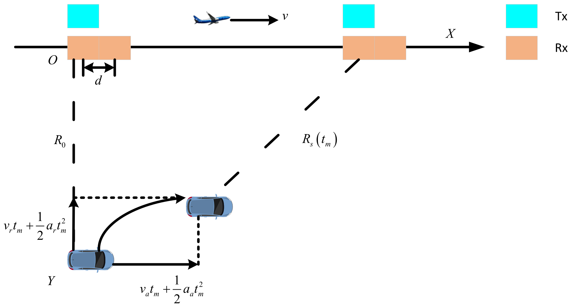
Figure 1 illustrates the geometry between the SAR platform and a ground maneuvering target in the slant range plane, where the X axis and Y axis represent the radar’s motion trajectory and range coordinate, respectively. The dual-channel SAR sensor operates in the side-looking mode with a strip. The platform flies along the X-axis direction at a constant speed v, and the array is divided into two channels with spacing d along the flight direction. In an observation scenario, a moving target located at maintains uniform acceleration motion. The parameters , , , and represent the velocity and acceleration information of the target along the cross-track and along-track directions, respectively. Assuming that the fore channel transmits the radar pulse signals and all channels receive them, according to the equivalent phase center principle, the radar channels can be equivalently modeled as operating in a monostatic mode with a spacing of .
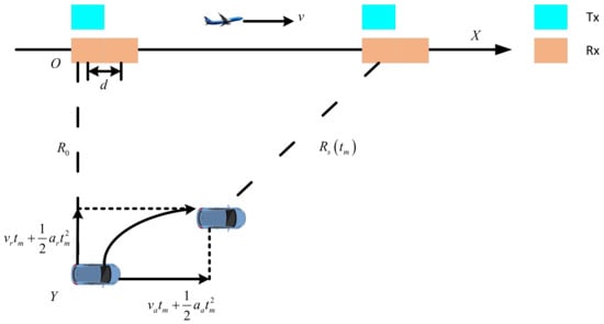
Figure 1.
Geometry relationship between a ground moving target and the SAR platform.
The instantaneous slant range between the i-th channel and the moving target can be expressed as
where is the spacing between the i-th received channel and the reference channel, and denotes the azimuth slow-time variable.
Assuming that a linear frequency modulated signal is transmitted during system operation, the echo signal of the moving target after range compression in the i-th channel can be written as
where t, , , , B, c, and denote the fast-time variable, the target complex reflectivity, the range compression gain, the slow-time window function, the range bandwidth, the speed of light, and the wavelength of the transmitted signal, respectively. Accordingly, the echo signal of the clutter after range compression in the i-th channel can be expressed as
where denotes the clutter complex reflectivity, and denotes the range from the clutter point to the i-th channel.
For SAR systems, the target signal is usually overwhelmed by clutter and cannot be distinguished by the receiver. Therefore, the echo signal of the i-th channel can be expressed as
where denotes the noise signal. According to (4), one can see that the target usually cannot be detected directly due to the interference of the clutter and noise. In order to improve the target output signal-to-clutter-and-noise ratio (SCNR), clutter suppression techniques are typically performed. Commonly used clutter suppression algorithms include STAP, DPCA, ATI, and ISTAP. By the way, it can be noticed that before clutter suppression, channel balancing should be implemented to compensate for channel errors caused by differences in antenna patterns and variations in electronic components. Taking the DPCA algorithm as an example, the processing flow can be expressed as
Substituting (2) and (3) into (5), it can be found that the difference in the echo signal between channels is mainly reflected in the slant range. Therefore, according to the Taylor series expansion around , the slant range difference of target between and can be formulated as (6). It can be found that the phase difference of the target signal between channels is caused by the target’s velocity, which makes the energy of the target preserved after clutter suppression.
According to (6), by setting both the velocity and acceleration of the target to zero, the expression for the clutter range difference can be derived, and . This means that the moving target signal will be maintained, while the clutter signal is suppressed through channel cancellation. Finally, (5) can be rewritten as
where represents amplitude of the target after DPCA, and , , and denote the equivalent first-, second-, and third-order coefficients, respectively. These coefficients can be expressed as [30]
It is worth noting that in (7), we have neglected the range migration caused by , as it typically does not exceed one range cell. From (7), it can be observed that there are three issues that need to be addressed before moving target parameter estimation:
- (1).
- Due to the impact of the velocity of target, the signal is remodeled as a cubic frequency modulation signal in the slow-time direction, rendering the conventional second-order signal model ineffective.
- (2).
- Due to the coupling between the fast-time range and slow-time azimuth, the target’s motion trajectory exhibits nonlinear range migration, resulting in an undesirable loss in the SCNR.
- (3).
- In the process of parameter estimation, clutter suppression reduces the spatial degrees of freedom in dual-channel radar systems. As a result, even after obtaining , , and , (8) remains as an underdetermined system and cannot accurately estimate the target’s cross-track and along-tarck velocity information.
In the next section, considering the aforementioned challenges, we propose a novel method for estimating the motion parameter information of the ground targets in a dual-channel radar system.
3. Proposed Algorithm Description
In this section, the procedures of the proposed algorithm for estimating the four-dimensional motion parameters of ground targets is described in detail. Additionally, considering the impact of channel balancing on the phase of moving targets, we have improved the channel balancing algorithm.
3.1. Channel Balancing
During the signal model analysis, we mentioned that inter-channel errors need to be corrected before clutter suppression. To deal with this issue, the adaptive 2D calibration (A2DC) algorithm has been proposed in [31]. Through iterative adjustments of the spectral response of the second channel to the reference channel one as in (9), the performance of the A2DC has been validated in many airborne and spaceborne SAR systems [32]. From (9), one can see that due to the integration and summation operation, the equalization process of the A2DC essentially involves estimating the error of strong energy sources, which is followed by calculating the compensation weights. In general, applying the A2DC algorithm effectively compensates for amplitude and phase errors between channels when the target signal’s energy is lower than that of the clutter. However, as the target energy increases, A2DC may distort the phase values of moving targets, thereby affecting the subsequent parameter estimation performance [33].
In order to deal with the issue, a modified A2DC (MA2DC) has been proposed in [33]. According to [33], it is known that the phase before channel balancing exhibits a linear relationship in the Doppler domain. Utilizing this characteristic, the MA2DC algorithm employs the least squares method to fit the linear slope along the Doppler domain and estimate the phase values of outlier values for compensation. The calibration weights in the Doppler domain can be expressed as
where is the phase obtained through linear fitting along the Doppler domain. However, in practical applications, we have observed that during the iterative process of the MA2DC algorithm, when the phase error between channels is large, linear fitting effectively compensates for the outlier phase values. As the iteration progresses and the phase error between channels decreases, the phase represented by the outlier values may cause a shift in the linear fitting, leading to overcompensation of the channel phase.
Therefore, from a data processing perspective, we introduce the random sample consensus (RANSAC) algorithm [34] to decrease the impact of outliers on phase fitting. The core idea of RANSAC is to iteratively select random samples from the dataset and evaluate the consistency of these samples to choose the optical model. This algorithm is particularly well suited for data with significant noise and outliers.
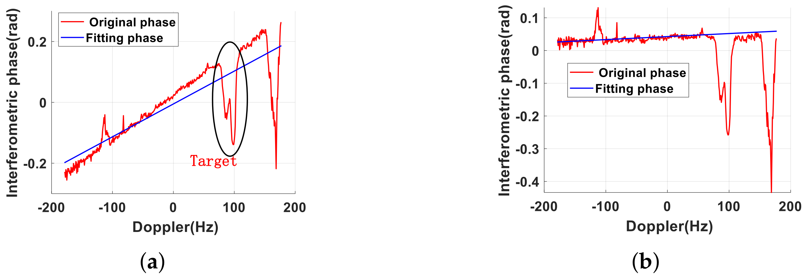
Figure 2a illustrates the fitting phase of the MA2DC algorithm proposed in [33] during the fifth iteration. The “original phase” represents the interference phase compensation value calculated using the A2DC algorithm. The “fitting phase” represents the interference phase compensation value calculated using the MA2DC algorithm through slope fitting. It can be observed that due to the influence of strong target energy, the fitting phase curve deviates from the clutter phase. When using the estimated phase to compensate for channel errors, it may lead to the distortion of the phase of the target. The Figure 2b shows the improved fitting phase curve of the MA2DC algorithm using the RANSAC algorithm presented in this paper. Compared to the A2DC, the proposed algorithm can mitigate the impact of outliers. Therefore, by introducing the RANSAC algorithm, it is possible to better correct inter-channel errors without affecting the phase of the target.
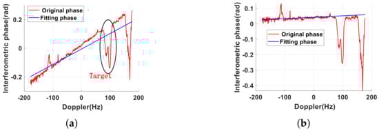
Figure 2.
The phase fitting results after the fifth iteration. (a) MA2DC. (b) MA2DC+RANSAC.
3.2. Range Cell Migration Compensation
After channel balancing and clutter cancellation, the energy of the target signal is preserved, allowing for the extraction of the target signal’s energy for parameter estimation. It can be observed from (7) that the coupling between azimuth slow-time and fast-time t results in a nonlinear shift of the target’s envelope, which includes its range walk, range curvature, and third-order range migration. Therefore, before estimating the target parameters, range migration correction needs to be performed. The KT [35] and SOKT [36] can be used to correct the first-order range walk and second-order range curvature, respectively, but they are unable to handle the migration caused by the third-order term. Additionally, the ambiguity of the velocity also limits the application of the KT. To address this issue, an interesting idea was proposed in [23], namely, the RFRT. Through the RFRT, arbitrary-order range migration correction can be achieved. After performing the range fast Fourier transform (FFT) on (7), one has the following:
where f represents the range frequency, and represents the signal amplitude after range FFT. Reversing the signal along the range frequency axis f, the RFRT can be expressed as
where the symbol “” above f represents the RFRT. can be noted as
where N denotes the number of points used for the FFT along the fast-time t. After multiplying (11) by (12), one has the following:
By applying the inverse Fourier transform to (14), the expression of the signal after the RFRT processing is obtained, which ca be expressed as
where represents the signal amplitude after the RFRT in the two-dimensional time domain. From (15), it can be noticed that after the RFRT, the range envelope of the target is corrected to the time .
However, we observe that during the application of the RFRT algorithm, the frequency axis is selected within the range . Considering the scenario where the signal sampling frequency is greater than the signal bandwidth, the chosen frequency range may introduce additional noise energy, as there is virtually no target energy outside the signal bandwidth. Assume that the energy of the target signal in the range frequency bin is and that the noise energy is . According to the appendix of [25], after applying the RFRT, the target’s SNR can be expressed as
where denotes the number of range frequencies corresponding to the signal bandwidth. According to (16), it can be found that the SNR decreases with increasing sampling frequency, which may worsen the performance of subsequent parameter estimation. Therefore, in practical applications, we perform RFRT on the signal in range bandwidth to reduce the SNR degradation caused by noise outside the bandwidth, that is,
After the improvement, the target’s SNR is rewritten as
Figure 3 illustrates the SNR curves obtained by applying RFRT over the sampling frequency and the signal bandwidth, respectively. It can be observed that as the sampling frequency increases, the advantage of the latter becomes increasingly evident.
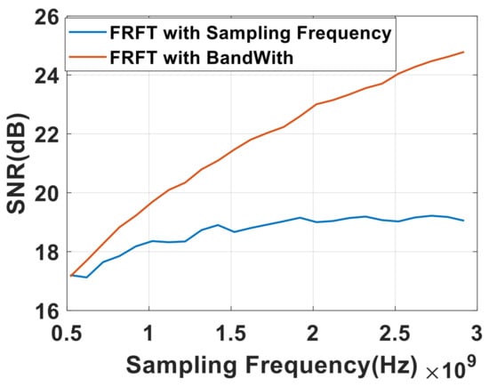
Figure 3.
Comparing the signal-to-noise Ratio (SNR) after applying RFRT using bandwidth and sampling frequency, respectively.
3.3. Polynomial Coefficient Estimation
From (15), after range migration correction, the coupling between t and is removed, and the target’s energy is focused along slow time into a single range cell of . Moreover, we can find that the target signal can be considered a cubic phase modulation (CPM) model along the azimuth slow time. To estimate the coefficients of a cubic polynomial, many methods have been developed, such as generalized Hough high-order ambiguity function (GHAF) [37], generalized radon Fourier transform (GRFT) [38], and radon-cubic phase function–Fourier transform (RCFT) [35]. These algorithms demonstrate excellent performance in polynomial parameter estimation.
With the development of nonuniform sampling techniques, the GSCFT method was proposed in [39]. Meanwhile, to reduce the impact of cross terms caused by multiple targets, we introduce an additional delay variable, allowing the energy of the interaction terms to diffuse across a two-dimensional space. Based on the nonlinear transformation proposed in [39], we have the following:
where ∗ and denote the complex conjugate symbols and delay variable, and is the fixed delay. According to [39], is set as 0.089 times the signal length. From (19), it is evident that after the nonlinear transformation, there is a coupling between the delay-time variable and the slow-time variable. When the FFT along slow time is performed, it can be observed that the signal energy will be distributed along , where denotes the frequency corresponding to .
To deal with this issue, [38] proposed the use of the Hough transform to accumulate target energy. However, the high complexity introduced by the Hough transform is unavoidable. In [39], the GSCFT was proposed, which can be realized through the Chirp-Z transform, significantly reducing computational complexity. The GSCFT expression is given as
where is the scaling factor, and represents the frequency corresponding to . Substituting into (20), one has
From (21), it can be noticed that the target energy is concentrated at along after the GSCFT. Next, performing a FFT along the , one has
where represents the frequency corresponding to . According to (22), after the aforementioned processing, the target will form a peak at . According to the peak detection technique, the second-order and third-order coefficients of the signal can be estimated as follows:
Based on the estimated values of and , we construct the compensation function , which can be expressed as
3.4. SAL Estimation
In the previous subsection, we estimated the polynomial coefficients of the target signal. However, after estimating the polynomial coefficients of the signal, there are still two main issues that need to be addressed for accurate estimation of the target parameters: (1). According to (8), it can be observed that there are four unknown variables related to the target’s motion parameters, while there are only three known equations. So, even with the polynomial coefficients obtained, the resulting equation remains underdetermined, making it impossible to accurately obtain the target’s motion parameters. (2). As discussed in [25], although the RFRT can correct for any-order range migration of the target, it also results in the loss of the target’s range information. Furthermore, the above analysis does not account for velocity ambiguity. When the target velocity exceeds the maximum unambiguous velocity allowed by the system, the value of parameter will not represent the true radial velocity of the target. To address these issues, we propose a windowed search compensation algorithm in this subsection.
When the impact of cross-track velocity ambiguity is considered, (11) can be rewritten as
where denotes the number of radial velocity ambiguities, denotes the blind velocity, denotes the baseband velocity, and denotes pulse repetition frequency (PRF). Using the polynomial parameters obtained in the above subsection, a compensation function can be constructed:
Multiplying by , and considering that , the signal is left with only range migration caused by Doppler ambiguity, that is,
For (28), a windowed search compensation function is proposed, which can be expressed as
where the window function is expressed as
where and represent the start time and end time of the search window, respectively. Figure 4 illustrates the relationship between the search window and the SAL. denotes the time that the target enters the radar range, and denotes the time that the target is out of radar range. It can be observed that the target signal can be fully extracted without introducing additional noise energy only when both conditions and are simultaneously satisfied. According to the target’s synthetic aperture time, we have a new variable equation
where L denotes synthetic aperture length of the radar system. Combining with (8), we can see that the number of equations in the system equals the number of unknown variables, thus making it possible to accurately obtain the velocity of the target.
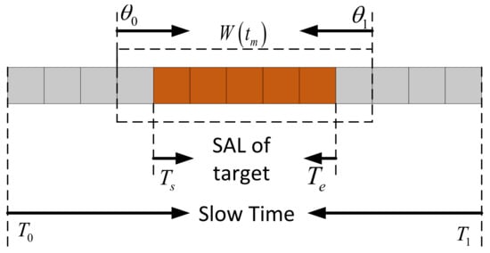
Figure 4.
The relationship between the search window length and the target’s SAL.
Multiplying by and performing the range IFFT, it can be noticed that when , the energy of the moving target is focused at . Not only can the range information of the target be obtained, but performing an FFT along slow time will also effectively focus the target’s energy. The processing flow can be expressed by (32):
The search window function ensures the accumulation of both the target energy and noise energy during the time interval -. Therefore, the output SNR of the is discussed considering different values of and . Assume that the target energy and noise energy after compensation using are given by and , respectively.
Case 1. or .
In this case, due to the window function not containing the signal energy, the SNR of the target may approach an infinitesimally small value, that is,
Case 2. and .
According to Figure 4, in Case 2, in addition to the accumulation of the target and noise components within the interval , additional noise energy within the intervals and is introduced. After compensation, the output SNR is now
where denotes the number of accumulated pulses in the SAL of the target, and denotes the number of accumulated pulses in the search time.
Case 3. and .
When the search window time falls within the synthetic aperture time of the target, since no additional noise energy is introduced, the output SNR is expressed as
Specifically, when and , the output SNR is now
Case 4. and .
Under this assumption, the selection range of the search window not only fails to accumulate the entire signal energy but also introduces additional noise energy. The output SNR is
where denotes the number of accumulated pulses in Case 4.
Case 5. and .
Similar to Case 3, the output SNR is expressed as
where denotes the number of accumulated pulses in Case 5.
Based on the analysis of the output SNR under the various conditions mentioned above, we can conclude that the output SNR reaches its maximum value only when and . Finally, the polynomial coefficients of the signal and SAL of target can be estimated as
3.5. Parameter Estimation of Moving Target
In this subsection, we will use the previously obtained polynomial coefficients and SAL of a target to calculate its motion parameters. The equations related to the target parameter can be expressed as
According to and , the analytical solution of the target’s azimuth velocity is expressed as (41)
From (41), we can find that the target’s azimuth velocity appears to have two possible values. However, in practical applications, the target’s velocity usually has only one true value. We will now need to discuss each of the two possible values separately. Based on the Taylor series expansion, one has
Therefore, (41) can be rewritten as
From (43), we obtain the approximate value for the two possible velocity values of the target. For the former, the calculated target’s azimuthal velocity is close to the platform’s velocity. However, the along-track velocity of the ground moving targets is typically much lower than that of the platform. Therefore, it is reasonable to exclude the first value. The final parameter estimate is then expressed as
3.6. Performance Analysis
(1) Multiple Ground Moving Target Parameter Estimation: In the discussion above, a novel parameter estimation algorithm for ground target is proposed, which can obtain the four-dimensional parameter information of the moving target. In practical applications, the presence of multiple ground maneuvering targets within a single or adjacent range cell is inevitable. The cross interference caused by the nonlinear transform of the RFRT and GSCFT needs to be considered. In the following, the parameter estimation effectiveness of multiple moving targets will be analyzed. Assuming there are moving targets in the observation scene, the signal of the targets can be expressed according to (15) in the range–frequency domain as follows:
Then, after the RFRT, one has
For (48), after RFRT processing, range migration still persists, with the energy of the cross terms distributed across different range units. The interference from the cross terms caused by the RFRT can be ignored. Therefore, when extracting the signal corresponding to , the signal expression is given by
where represents the signal energy after the RFRT. Reference [39] provides a detailed analysis of the cross-term effects caused by the subsequent nonlinear transformations; here, we only present the conclusion. After performing the FFT along and , the cross-terms energy will defocus in the two-dimensional space due to the complex coupling between their phase and amplitude. Compared to the auto-correlation energy, these cross terms can be considered negligible. When the strong and weak targets coexist, the “CLEAN” technique [40] technique can effectively reduce the impact of strong target cross terms on the weak target’s auto-terms.
(2) Computational Complexity Analysis: Assume that the numbers of azimuth pulses and range gates are denoted by and , respectively. Based on the principle of the proposed method, the complexity of the proposed algorithm is primarily reflected in the RFRT with the computational cost of , parametric autocorrelation function , GSCFT , and FFT operation along the uniform lag-time axis . Thus, its computational cost is also in the order of the .
4. Simulation and Real Data Processing Results
In this section, the simulated results and the processing results of several real SAR datasets are used to analyze the effectiveness of the proposed algorithm.
4.1. Simulation Results
(1) Multiple Ground Moving Target Parameter Estimation: In this subsection, multiple targets were considered in the simulation to discuss the effectiveness of the proposed algorithm. Assuming that a radar platform with two spatial channels is flying at a constant speed along a predetermined flight trajectory, and were considered in this simulation. Table 1 gives the simulated SAR system parameters.

Table 1.
Simulation system parameters.
The motion envelopes of and after range compression are shown in Figure 5a. From Figure 5a, it is observed that complex range migrations occurred for these targets. In addition, distinguishing the target trajectories using range segmentation techniques became a challenge due to the cross of these targets’ motion trajectories. Figure 5b shows the result in the range–frequency domain and azimuth–time domain after performing FFT along the fast-time axis. It can be observed that the signal energy is only present within the range bandwidth, while the remaining areas are entirely occupied by noise energy. The application of the FRFT with the sampling frequency may result in additional noise energy being introduced. Figure 5c,d shows the two-dimensional time domain result after range migration correction. In addition to the self-focusing term at time in the range cell, there are also two slanted lines caused by cross terms. However, since the energy of the cross terms is dispersed along the range axis, the cross interference can be ignored when extracting the self-focusing term. After applying the GSCFT, two well-focused targets are shown in the two-dimensional time domain.

Figure 5.
Multiple target processing results. (a) The trajectory of targets. (b) The results of FFT along fast time. (c) RCMC by RFRT. (d) Cross interference of RFRT. (e) The results of GSCFT.
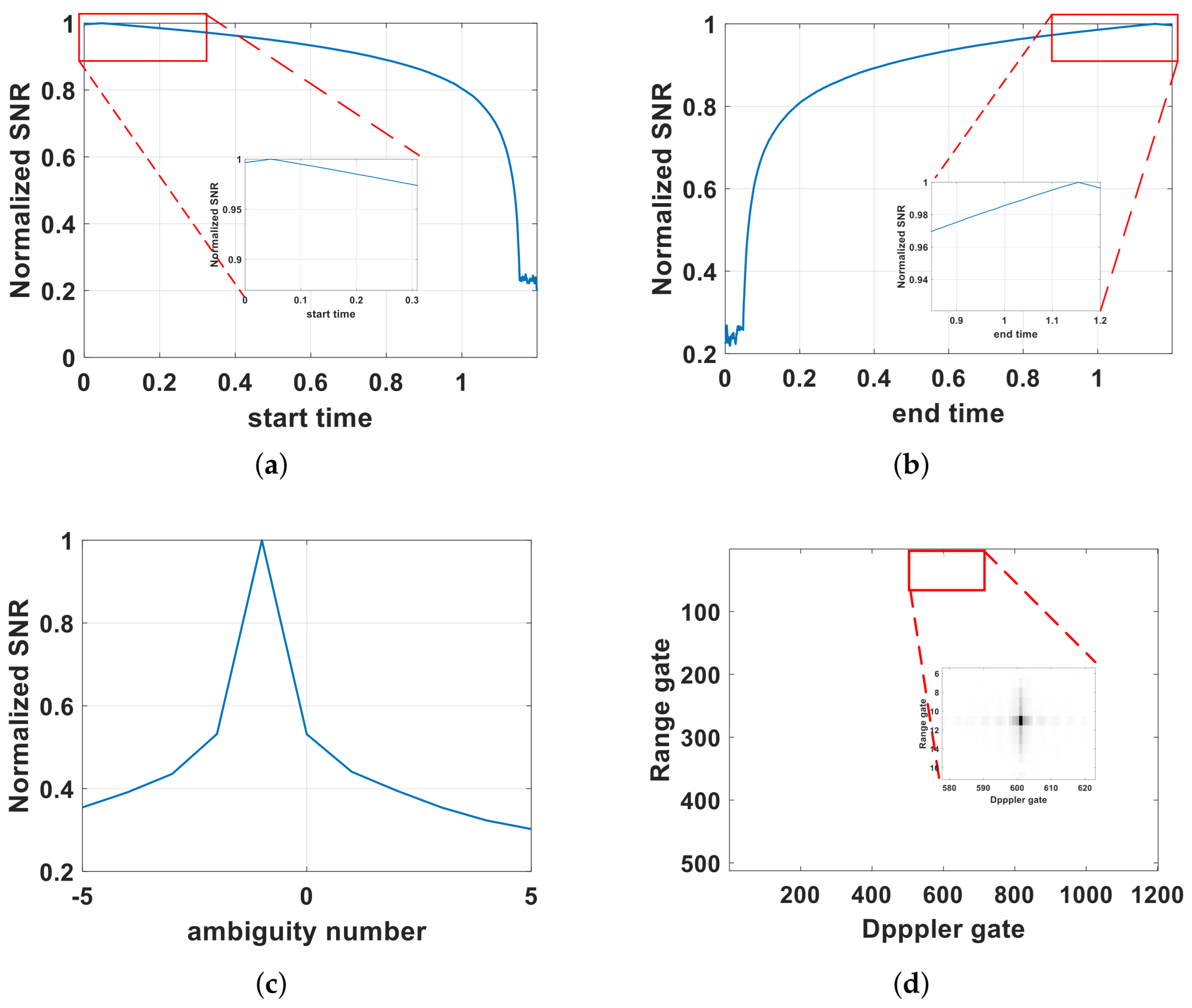
The Figure 6a,b shows the synthetic aperture time estimation result for the . Consistent with theoretical analysis, the target’s output signal-to-noise ratio (SNR) reached its maximum only when the search window satisfied and . Additionally, considering the potential Doppler ambiguity, Figure 6c,d show the Doppler ambiguity search results and the final two-dimensional time domain focusing result. Furthermore, Table 2 and Table 3 present the polynomial coefficients and motion parameter results for .
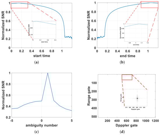
Figure 6.
The SAL estimation results and imaging results for Tar1. (a) Start time search result. (b) End time search result. (c) Ambiguity velocity search result. (d) Focusing result of Tar1.
Table 2.
The polynomial coefficients of Tar1.
Table 3.
The motion parameter of Tar1.
Similarly, Figure 7a,b shows the synthetic aperture time estimation result for . Figure 7c,d show the Doppler ambiguity search results and the final two-dimensional time domain focusing result. Table 4 and Table 5 present the polynomial coefficients and motion parameter results for . By comparing the parameter estimation results with the true values, it can be observed that the proposed algorithm not only effectively suppresses the influence of cross terms but also achieves four-dimensional motion parameter estimation in a single-channel scenario.
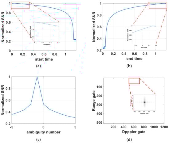
Figure 7.
The SAL estimation results and imaging results for Tar2. (a) Start time search result. (b) End time search result. (c) Ambiguity velocity search result. (d) Focusing result of Tar2.
Table 4.
The polynomial coefficients of Tar2.
Table 5.
The motion parameter of Tar2.
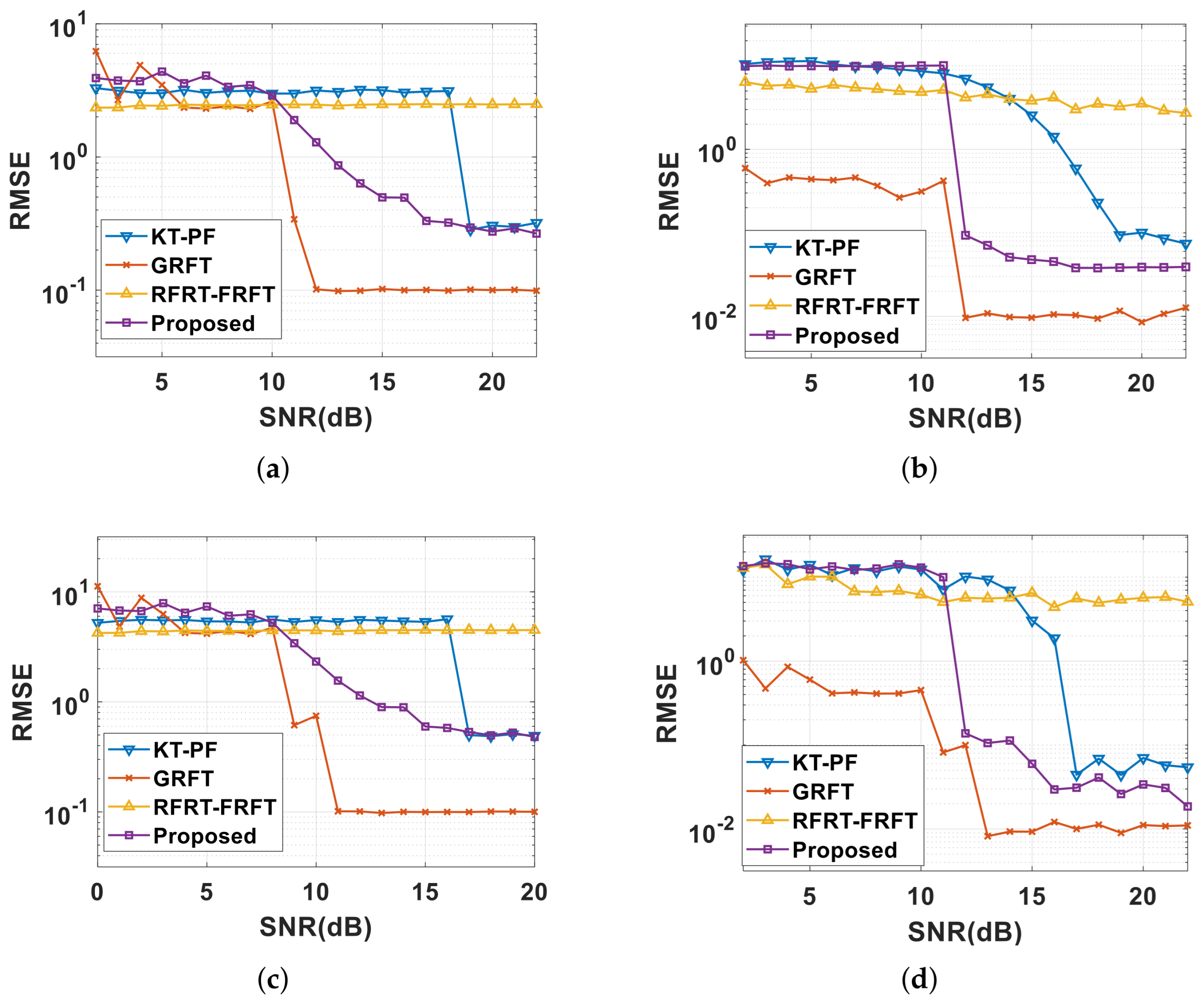
(2) The Accuracy of Target Parameter Estimation: In the above section, we proposed a method for estimating moving target velocity information using polynomial coefficients and the SAL. In practical applications, the accuracy of parameter estimation, as a crucial performance metric, needs to be thoroughly discussed. In the simulation, we included existing algorithms such as RFRT-FRFT [25], KT-PF [29], and GRFT [38] for comparison and discussion of the proposed algorithm’s parameter estimation performance. It is important to note that the GRFT algorithm, as a parameter search method, effectively estimates the polynomial coefficients of the target. However, it is unable to provide target velocity information for the underdetermined Equation (8) in the paper. To facilitate a better comparison of algorithm performance, we used the SAL algorithm proposed in this paper to estimate the target velocity based on the polynomial coefficients estimated by the GRFT.
Through multiple Monte Carlo experiments, we evaluated the parameter estimation performance of different algorithms. Figure 8a–d show the parameter estimation performance for the target’s cross-track velocity, cross-track acceleration, along-track velocity, and along-track acceleration. For the RFRT-FRFT algorithm, the lack of target cubic term coefficient estimation capability led to errors in the four-dimensional velocity estimation. For KT-PF, although it could estimate the four-dimensional parameters of the target, the polynomial fitting and Doppler bandwidth estimation required a high SNR, which resulted in good parameter estimation performance only under high SNR conditions. As for the proposed algorithm, compared to KT-PF, it not only providesd better parameter estimation performance but also demonstrated accurate parameter estimation when the SNR exceeded 12 dB. For GRFT, due to its use of a three-dimensional parameter search method to obtain polynomial coefficients, it performed well under low SNR conditions but incurred a significant increase in computational complexity. The proposed algorithm, in contrast, has lower computational complexity than GRFT, making it more suitable for real-time applications where system responsiveness is critical.
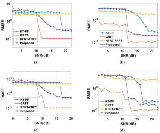
Figure 8.
The estimation performance of motion parameter. (a) Cross-track velocity. (b) Cross-track acceleration. (c) Along-track velocity. (d) Along-track acceleration.
4.2. Real Data with Ku-Band
In this subsection, we will demonstrate the effectiveness of the algorithm by processing real data from an airborne dual-channel SAR radar. The observed scene was selected as a highway in an urban area, which is beneficial for discussing the accelerated motion of targets. The radar system operated in the Ku-band, with specific parameters listed in Table 6.
Table 6.
SAR system parameters.
Before clutter suppression, a channel balancing algorithm needed to be performed. Figure 9 shows the interference phase results of the MA2DC compared to our proposed method. In Figure 9a, a deep blue line along the range gate is evident within the interference phase, as highlighted in the red box, indicating the potential presence of a strong target, which may degrade equalization performance. In Figure 9b, after applying the proposed method, the blue line in the red box disappeared, demonstrating the effectiveness of the channel equalization algorithm in enhancing channel correlation while avoiding phase distortion of moving targets caused by MA2DC.
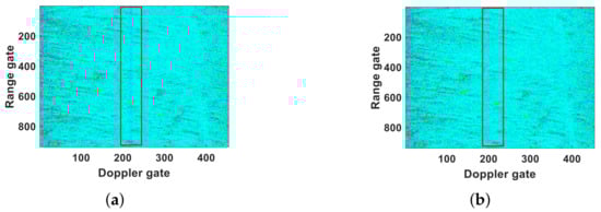
Figure 9.
The interference phase results after processing by different channel balancing algorithms. (a) MA2DC. (b) RANSAC+MA2DC.
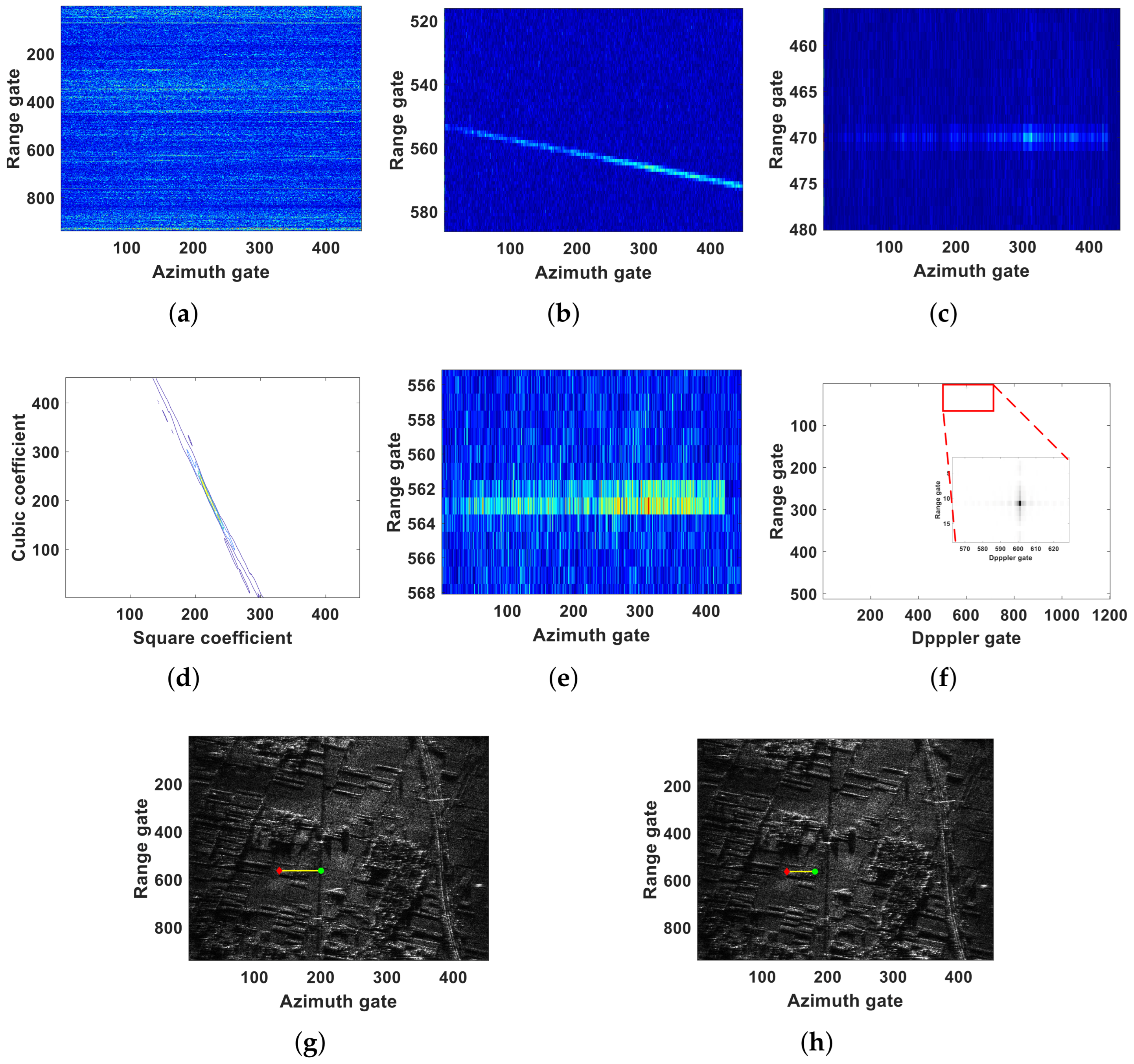
Figure 10a shows the two-dimensional time domain echo signal after channel balancing. Due to the interference of ground clutter, the target signal was overwhelmed by the clutter signal, making it difficult to detect. After clutter suppression, Figure 10b shows the results after clutter suppression, where the clutter energy was effectively suppressed. Additionally, range migration trajectories caused by multiple uncooperative maneuvering targets in the observed scene are evident. After extracting the moving target signals following clutter suppression and performing the RFRT, the range migration of the targets was fully compensated, as shown in Figure 10c. Figure 10d illustrates the estimation results of the quadratic and cubic terms of the target. It is evident that, after clutter suppression, the influence of cross terms was nearly nonexistent, allowing for effective estimation of the target’s polynomial parameters. After compensation with (30), the target energy formed a well-focused peak in the two-dimensional time domain, as shown in Figure 10f. Furthermore, utilizing the estimated radial velocity, we could achieve target relocation in Figure 10g, where the azimuth offset pixel of the target could be calculated using . To demonstrate the impact of MA2DC on the target’s phase, we present in Figure 10h the relocated results of the target through the MA2DC algorithm. In contrast to Figure 10g, the relocation results in Figure 10h did not position the target on the road, while Figure 10g successfully located the target on the highway, highlighting the effectiveness of the proposed algorithm.
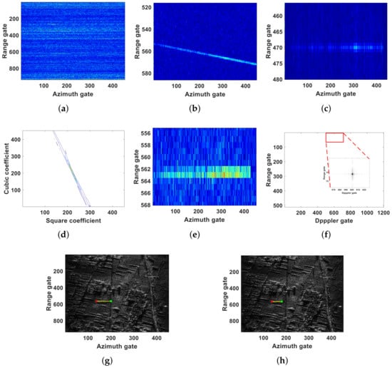
Figure 10.
Parameter estimation results of the proposed algorithm in a dual-channel airborne SAR system. (a) Two-dimensional time domain result before clutter suppression. (b) Target motion trajectory after clutter rejection. (c) RCMC result by RFRT. (d) GSCFT result. (e) RCMC results after the compensation function. (f) Final focusing result by the proposed method. (g) Moving target relocation result after proposed method. (h) Moving target relocation result after MA2DC. (The red diamond represents the detection result of the moving target, and the green circle represents the relocation result of the moving target).
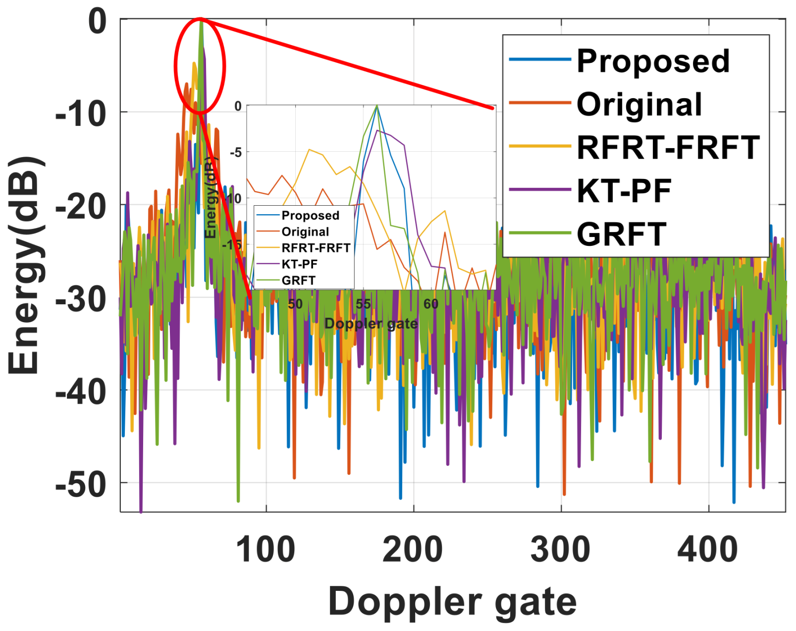
In Figure 10, we show the parameter estimation performance of the proposed algorithm. Next, we aimed to further highlight the algorithm’s performance through a comparison with existing algorithms. From Figure 11, it can be seen that the GRFT and the proposed algorithm both exhibited good focusing performance. However, it should be noted that GRFT employs a three-dimensional search approach, which introduces significant computational complexity. Furthermore, with regard to (44), the GRFT is only capable of estimating polynomial coefficients and does not possess the ability to estimate the four-dimensional target parameters.
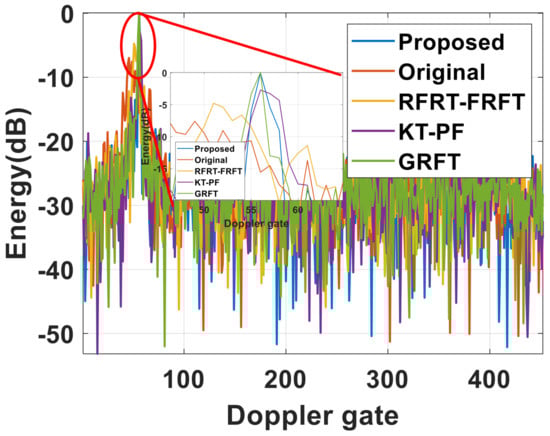
Figure 11.
Focusing results of different algorithms with Ku-band.
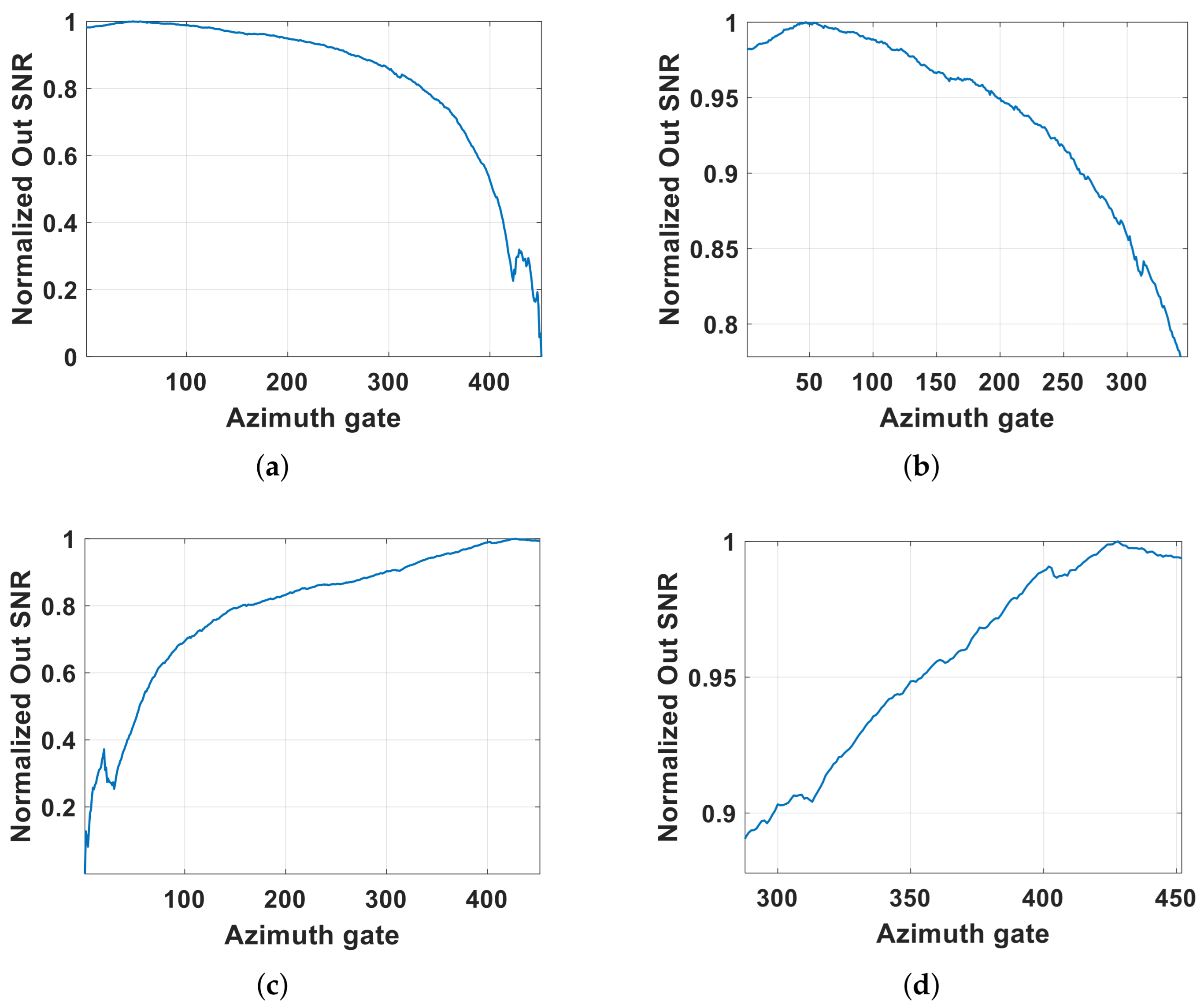
However, merely estimating the polynomial coefficients of the target signal is insufficient to obtain the target’s four-dimensional velocity information. According to the analysis in Section 3, we introduced the target’s SAL to further constrain the parameter equations. Figure 12 shows the estimated SAL results obtained using the maximum output SNR, including the target’s start and end times. By utilizing the estimated SAL, we were able to calculate the target’s four-dimensional motion parameter, as shown in Table 7. Although the true motion parameters of the target could not be determined, both the effective refocusing results of the target in the measured data and the consistency between the SNR variation trend in the SAL estimation, as well as the theoretical analysis, ensured the effectiveness of the proposed algorithm.
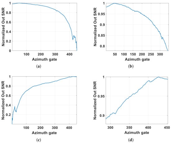
Figure 12.
SAL results of ground moving target. (a) Start time search result. (b) Start time search local result. (c) End time search result. (d) End time search local result.
Table 7.
The motion parameter estimation of moving target.
Additionally, to more intuitively demonstrate the performance of the proposed algorithm, we have included a comparison with existing algorithms. The image entropy, as a metric for assessing target focusing performance, has been introduced. The expression of the image entropy is
where is the total power of the image pixels, and is the index of the image pixel. Table 8 shows the target image entropy after processing by different methods. It demonstrates the fact that the proposed method has the lowest image entropy, which indicates that the proposed method offers a better focusing performance.
Table 8.
Entropy of different methods.
4.3. Real Data with X-Band
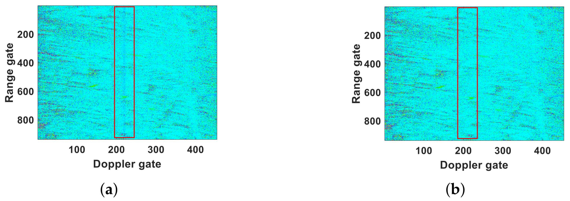
In this section, another set of dual-channel SAR real data, with an urban road as the observation scene, is used to further demonstrate the performance of the proposed algorithm. The specific parameters listed in Table 9. Although the target moves rapidly within the scene, due to the limitations of the antenna size, the ground moving target with velocity ambiguity is still submerged in the main lobe clutter, as shown in Figure 13a. After clutter suppression, the results in the range–Doppler domain indicate that due to the complex motion of the target, its energy spread across different ranges and Doppler bins, as shown in Figure 13b.
Table 9.
SAR system parameters.
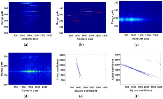
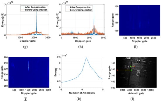
Figure 13.
Parameter estimation results results for two ground moving targets in a real airborne SAR system. (a) Range–Doppler domain results before clutter suppression. (b) Range–Doppler domain result after clutter suppression. (c) RCMC result of target1 by RFRT. (d) RCMC result of target 2 by RFRT. (e) GSCFT result of target 1 (f) GSCFT result of target 2. (g) The result of compensating of target 1 after Equation (30). (h) The result of compensating of target 2 after Equation (30). (i) Final focusing result of target 1 by the proposed method. (j) Final focusing result of target 2 by the proposed method. (k) Ambiguity search result of target’s radial velocity. (l) Relocation result of targets. (The red diamond represents the detection result of the moving target, and the green circle represents the relocation result of the moving target).
After RFRT processing, the range migration of the targets was well corrected, as shown in Figure 13c,d. By compensating the target signal using the second-order and third-order coefficients of the target estimated through the GSCFT, the targets-focusing effects shown in Figure 13g,h were achieved. From Figure 13g,h, it can be observed that compared to the energy defocusing caused by Doppler spreading before compensation, the compensated target signal effectively focused the target energy, demonstrating the effectiveness of the parameter estimation algorithm. The final focused result is shown in Figure 13i,j. Incidentally, Figure 13k also shows the Doppler ambiguity search result for target 2. Based on the estimated radial velocity of the target, the relocation result of the target is shown in Figure 13l. Finally, the estimated velocity information of targets is presented in Table 10.
Table 10.
The motion parameter estimation of moving target.
The range profile results for multitargets in the X-band are shown in Figure 14. By comparing with existing algorithms, it can be observed that the focusing performance of the proposed algorithm is similar to that of the GRFT algorithm. Table 11 presents a comparison of image entropy values for multitargets in the X-band. It can be observed that the GRFT exhibited lower image entropy values due to its multidimensional parameter search. The proposed algorithm showed significantly lower image entropy values compared to the results of RFRT-FRFT and KT-PF. This indicates that the proposed algorithm outperformed the other algorithms in terms of parameter estimation performance.
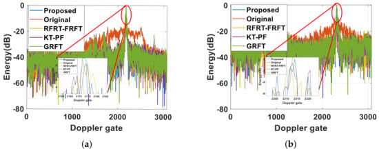
Figure 14.
Focusing results of different algorithms with X-band. (a) Target 1. (b) Target 2.
Table 11.
Entropy of different methods with X-band.
5. Discussion
In the previous section, we analyzed the performance of the proposed algorithm through simulations and real-world data processing results. The simulation results show that the proposed algorithm outperforms RFRT-FRFT and KT-PF in terms of parameter estimation performance. When the SNR exceeds 12 dB, the parameter estimation results become increasingly accurate. Compared to the GRFT algorithm, the proposed algorithm has a lower computational complexity, making it more suitable for practical engineering applications. The real-world data results not only validate the correctness of the theoretical derivations, confirming that the target’s SAL can be estimated using the maximum output SNR criterion, but also demonstrate, through the comparison of image entropy values, that the proposed algorithm can achieve precise target focusing and improve the target’s output SCNR.
6. Conclusions
In this study, we proposed a dual-channel SAR ground moving target parameter estimation algorithm designed to address the challenge of accurately estimating four-dimensional motion parameters after clutter suppression. Focusing on motion parameter estimation, we discussed channel equalization, range walk correction, polynomial estimation, and SAL estimation, and we proposed a comprehensive algorithm suitable for dual-channel SAR systems. Furthermore, we analyzed the performance of the proposed algorithm and demonstrated through simulations that it has robust parameter estimation capabilities when the SNR exceeds 12 dB. Finally, two real datasets were used to verify the effectiveness of the proposed algorithm.
Author Contributions
Conceptualization, K.L. and X.H.; methodology, K.L.; software, K.L. and G.L.; validation, S.Z. and C.Z.; formal analysis, K.L. and X.H.; investigation, K.L. and G.L.; resources, X.H.; data curation, K.L.; writing—original draft preparation, K.L.; writing—review and editing, K.L., X.H. and G.L.; visualization, X.H.; supervision, G.L.; project administration, G.L.; funding acquisition, G.L. and X.H. All authors have read and agreed to the published version of the manuscript.
Funding
This work was supported by the National Nature Science Foundation of China (NSFC) under Grant 62201408, Grant 61931016, Grant 62431021, and Grant 61621005.
Data Availability Statement
The original contributions presented in this study are included in the article. Further inquiries can be directed to the corresponding author.
Conflicts of Interest
The authors declare no conflicts of interest.
References
- Raney, R.K. Synthetic aperture imaging radar and moving targets. IEEE Trans. Aerosp. Electron. Syst. 1971, AES-7, 499–505. [Google Scholar] [CrossRef]
- Li, G.; Xu, J.; Peng, Y.N.; Xia, X.-G. Location and imaging of moving targets using nonuniform linear antenna array SAR. IEEE Trans. Aerosp. Electron. Syst. 2007, 43, 1214–1220. [Google Scholar]
- Huang, Y.; Liao, G.; Xu, J.; Li, J. GMTI and parameter estimation via time-Doppler chirp-varying approach for single-channel airborne SAR system. IEEE Trans. Geosci. Remote Sens. 2017, 55, 4367–4383. [Google Scholar] [CrossRef]
- Chen, X.; Yu, X.; Huang, Y.; Guan, J. Adaptive clutter suppression and detection algorithm for radar maneuvering target with high-order motions via sparse fractional ambiguity function. IEEE J. Sel. Topics Appl. Earth Observ. Remote Sens. 2020, 13, 1515–1526. [Google Scholar] [CrossRef]
- Huang, P.; Zhang, X.; Zou, Z.; Liu, X.; Liao, G.; Fan, H. Road-aided along-track baseline estimation in a multichannel SAR-GMTI system. IEEE Geosci. Remote Sens. Lett. 2021, 18, 1416–1420. [Google Scholar] [CrossRef]
- Perry, R.P.; DiPietro, R.C.; Fante, R.L. SAR imaging of moving targets. IEEE Trans. Aerosp. Electron. Syst. 1999, 35, 188–200. [Google Scholar] [CrossRef]
- Chen, J.; Xu, X.; Zhang, J.; Xu, G.; Zhu, Y.; Liang, B. Ship Target Detection Algorithm Based on Decision-Level Fusion of Visible and SAR Images. IEEE J. Miniaturization Air Space Syst. 2023, 4, 242–249. [Google Scholar] [CrossRef]
- Huang, H.; Huang, P.; Liu, X.; Xia, X.; Deng, Y.; Fan, H. A novel channel errors calibration algorithm for multichannel high-resolution and wide-swath SAR imaging. IEEE Trans. Geosci. Remote Sens. 2022, 60, 5201619. [Google Scholar] [CrossRef]
- Dragosevic, M.; Burwash, W.; Chiu, S. Detection and estimation with RADARSAT-2 moving-object detection experiment modes. IEEE Trans. Geosci. Remote Sens. 2012, 50, 3527–3543. [Google Scholar] [CrossRef]
- Huang, P.; Liao, G.; Yang, Z.; Xia, X.-G.; Ma, J.-T.; Zhang, X. A Fast SAR Imaging Method for Ground Moving Target Using a Second-Order WVD Transform. IEEE Trans. Geosci. Remote Sens. 2016, 54, 1940–1956. [Google Scholar] [CrossRef]
- Werninghaus, R.; Buckreuss, S. The TerraSAR-X mission and system design. IEEE Trans. Geosci. Remote Sens. 2010, 48, 606–614. [Google Scholar] [CrossRef]
- Suess, M.; Riegger, S.; Pitz, W.; Werninghaus, R. TerraSAR-XDesign and performance. Proc. EUSAR 2002, 2, 49–52. [Google Scholar]
- Nohara, T.J.; Weber, P.; Premji, A.; Livingstone, C. SAR-GMTI processing with Canadas Radarsat 2 satellite. In Proceedings of the IEEE Adaptive Systems for Signal Processing, Communications, and Control Symposium, Lake Louise, AB, Canada, 4 October 2000; pp. 379–384. [Google Scholar]
- Thompson, A.; Livingstone, C. Moving target performance for RADARSAT-2. In Proceedings of the IEEE 2000 International Geoscience and Remote Sensing Symposium, Taking the Pulse of the Planet: The Role of Remote Sensing in Managing the Environment, Honolulu, HI, USA, 24–28 July 2000; pp. 2599–2601. [Google Scholar]
- Wang, C.; Liao, G.; Zhang, Q. First spaceborne SAR-GMTI experimental results for the Chinese Gaofen-3 dual-channel SAR sensor. Sensors 2017, 17, 2683. [Google Scholar] [CrossRef] [PubMed]
- Ender, J.H. Space-time adaptive processing for synthetic aperture radar. In Proceedings of the IEE Colloquium on Space-Time Adaptive Processing, London, UK, 6 April 1998. [Google Scholar]
- Duan, K.; Xu, H.; Yuan, H.; Xie, H.; Wang, Y. Reduced-DOF three-dimensional STAP via subarray synthesis for nonsidelooking planar array airborne radar. IEEE Trans. Aerosp. Electron. Syst. 2020, 56, 3311–3325. [Google Scholar] [CrossRef]
- Lightstone, L.; Faubert, D.; Rempel, G. Multiple phase centre DPCA for airborne radar. In Proceedings of the 1991 IEEE National Radar Conference, Los Angeles, CA, USA, 12–13 March 1991; pp. 36–40. [Google Scholar]
- Chapin, E.; Chen, C.W. Airborne along-track interferometry for GMTI. IEEE Aerosp. Electron. Syst. Mag. 2009, 24, 13–18. [Google Scholar] [CrossRef]
- Budillon, A.; Gierull, C.H.; Pascazio, V.; Schirinzi, G. Along-Track interferometric SAR systems for ground-moving target indication: Achievements potentials and outlook. IEEE Geosci. Remote Sens. Mag. 2020, 8, 46–63. [Google Scholar] [CrossRef]
- Cerutti-Maori, D.; Sikaneta, I. Optimum GMTI processing for space-based SAR/GMTI systems—Simulation results. In Proceedings of the 8th European Conference on Synthetic Aperture Radar, Aachen, Germany, 7–10 June 2010. [Google Scholar]
- He, X.; Liao, G.; Zhu, S.; Xu, J.; Guo, Y.; Wei, J. Fast non-searching method for ground moving target refocusing and motion parameters estimation. Digit. Signal Process. 2018, 79, 152–163. [Google Scholar] [CrossRef]
- Chen, X.L.; Guan, J.; Liu, N.B.; He, Y. Maneuvering target detection via radon-fractional Fourier transform-based long-time coherent integration. IEEE Trans. Signal Process. 2014, 62, 939–953. [Google Scholar] [CrossRef]
- Zhang, X.; Liao, G.; Zhu, S.; Yang, D.; Du, W. Efficient compressed sensing method for moving-target imaging by exploiting the geometry information of the defocused results. EEE Geosci. Remote Sens. Lett. 2015, 12, 517–521. [Google Scholar] [CrossRef]
- Huang, P.; Xia, X.-G.; Gao, Y.; Liu, X.; Liao, G.; Jiang, X. Ground moving target refocusing in SAR imagery based on RFRT-FrFT. IEEE Trans. Geosci. Remote Sens. 2019, 57, 5476–5492. [Google Scholar] [CrossRef]
- Zhu, S.; Liao, G.; Yang, D.; Tao, H. A new method for radar high-speed maneuvering weak target detection and imaging. IEEE Geosci. Remote Sens. Lett. 2014, 11, 1175–1179. [Google Scholar]
- Yang, J.; Liu, C.; Wang, Y. Imaging and parameter estimation of fast-moving targets with single-antenna SAR. IEEE Geosci. Remote Sens. Lett. 2014, 11, 529–533. [Google Scholar] [CrossRef]
- Sharma, J.J.; Gierull, C.H.; Collins, M.J. Compensating the effects of target acceleration in dual-channel SAR-GMTI. Proc. Inst. Electr. Eng.-Radar Sonar Navig. 2006, 153, 53–62. [Google Scholar] [CrossRef]
- Zhu, S.; Liao, G.; Tao, H.; Yang, Z. Estimating ambiguity-free motion parameters of ground moving targets from dual-channel SAR sensors. IEEE J. Sel. Top. Appl. Earth Observ. Remote Sens. 2014, 7, 3328–3349. [Google Scholar] [CrossRef]
- Zeng, C.; Li, D.; Luo, X.; Song, D.; Liu, H.; Su, J. Ground maneuvering targets imaging for synthetic aperture radar based on second-order keystone transform and high-order motion parameter estimation. IEEE J. Sel. Top. Appl. Earth Observ. Remote Sens. 2019, 12, 4486–4501. [Google Scholar] [CrossRef]
- Ender, J. The airborne experimental multi-channel SAR-system AERII. Proc. EUSAR 1996, 96, 49–52. [Google Scholar]
- Makhoul, E.; Baumgartner, S.V.; Jäger, M.; Broquetas, A. Multichannel SAR-GMTI in maritime scenarios with F-SAR and TerraSAR-X sensors. IEEE J. Sel. Top. Appl. Earth Observ. Remote Sens. 2015, 8, 5052–5067. [Google Scholar] [CrossRef]
- Ge, B.; An, D.; Liu, J.; Feng, D.; Chen, L.; Zhou, Z. Modified adaptive 2-D calibration algorithm for airborne multichannel SAR-GMTI. IEEE Geosci. Remote Sens. Lett. 2023, 20, 4004805. [Google Scholar] [CrossRef]
- Chum, O.; Matas, J. Optimal randomized RANSAC. IEEE Trans. Pattern Anal. Mach. Intell. 2008, 30, 1472–1482. [Google Scholar] [CrossRef] [PubMed]
- Zhu, D.Y.; Li, Y.; Zhu, Z.D. A keystone transform without interpolation for SAR ground moving-target imaging. IEEE Geosci. Remote Sens. Lett. 2007, 4, 18–22. [Google Scholar] [CrossRef]
- Zhou, F.; Wu, R.B.; Xing, M.D.; Bao, Z. Approach for single channel SAR ground moving target imaging and motion parameter estimation. IET Radar Sonar Navigat. 2007, 1, 59–66. [Google Scholar] [CrossRef]
- Huang, P.H.; Liao, G.S.; Yang, Z.W.; Xia, X.; Ma, J.T.; Zheng, J.B. Ground maneuvering target imaging and high-order motion parameter estimation based on second-order keystone and generalized Hough-HAF transform. IEEE Trans. Geosci. Remote Sens. 2017, 55, 320–335. [Google Scholar] [CrossRef]
- Xu, J.; Xia, X.-G.; Peng, S.; Yu, J.; Peng, Y.; Qian, L. Radar maneuvering target motion estimation based on generalized Radon-fourier transform. IEEE Trans. Signal Process. 2012, 60, 6190–6201. [Google Scholar]
- Zheng, J.; Liu, H.; Liao, G.; Su, T.; Liu, Z.; Liu, Q. ISAR imaging of targets with complex motions based on a noise-resistant parameter estimation algorithm without nonuniform axis. IEEE Sens. J. 2016, 16, 2509–2518. [Google Scholar] [CrossRef]
- Misiurewicz, J.; Kulpa, K.S.; Czekala, Z.; Filipek, T.A. Radar detection of helicopters with application of CLEAN method. IEEE Trans. Aerosp. Electron. Syst. 2012, 48, 3525–3537. [Google Scholar] [CrossRef]


Disclaimer/Publisher’s Note: The statements, opinions and data contained in all publications are solely those of the individual author(s) and contributor(s) and not of MDPI and/or the editor(s). MDPI and/or the editor(s) disclaim responsibility for any injury to people or property resulting from any ideas, methods, instructions or products referred to in the content. |
© 2025 by the authors. Licensee MDPI, Basel, Switzerland. This article is an open access article distributed under the terms and conditions of the Creative Commons Attribution (CC BY) license (https://creativecommons.org/licenses/by/4.0/).