Clutter Modeling and Characteristics Analysis for GEO Spaceborne-Airborne Bistatic Radar

Abstract

The spaceborne-airborne bistatic radar (SABR) system employs a spaceborne transmitter and an airborne receiver, offering significant advantages, such as wide coverage, outstanding anti-stealth capabilities, and notable resistance to jamming. However, SABR operates in a downward-looking configuration, and due to the separation of the transmitter and receiver, non-side-looking array reception, and the effects of Earth’s rotation, clutter exhibits both spatial-temporal coupling and distance dependence. These factors cause substantial expansion in spatial and temporal frequency domains, leading to severe degradation in radar detection performance for moving targets. This paper establishes an SABR clutter signal model that applies to arbitrary geometric configurations to respond to these challenges. The paper uses this model to analyze the non-side-looking clutter characteristics in a geostationary spaceborne-airborne bistatic radar configuration. Furthermore, the paper investigates the impact of various observation areas and geometric configurations on detection performance, using SCNR loss as the performance index. Finally, this paper gives suggestions on the transceiver’s geometric configuration and the observation area selection.

1. Introduction

With their elevated platform altitude and independence from national boundaries, spaceborne radar systems have garnered significant attention for their ability to deliver extensive coverage and persistent monitoring. However, the problems posed by significant signal power attenuation over vast distances, vulnerability to deliberate jamming during trajectory determination, and the presence of intensive ground clutter significantly complicate and present substantial challenges to the effectiveness of radar systems in performing reliable target detection missions [1,2,3]. Compared to conventional spaceborne radar systems, the spaceborne-airborne bistatic radar (SABR) system leverages a satellite as the transmitter and an aircraft as the receiver, significantly shortening transmission distances and mitigating spatial signal attenuation. Furthermore, the bistatic geometric configuration enhances spatial diversity, enabling target observation from multiple perspectives, which, in turn, provides improved resistance to jamming and stealth technologies [4,5]. Additionally, the SABR system is more cost-effective compared to the spaceborne bistatic radar (SBR) system and possesses greater coverage than the airborne bistatic radar [6,7]. However, the Doppler frequency of SABR echoes is influenced not only by the Earth’s rotation but also by the co-modulation of the two platforms, leading to a more pronounced clutter spectrum broadening compared to the airborne bistatic radar (ABR). Furthermore, the ultra-long baseline of SABR, combined with the significant mismatch between the satellite transmitter’s broad coverage and the airborne receiver’s limited field of view, exacerbates the clutter spectrum truncation. Therefore, to enhance the detection performance of SABR, it is imperative to investigate star mechanism configurations that are conducive to detection and analyze clutter characteristics along with their spatiotemporal adaptive clutter suppression capabilities across various star mechanism configurations, thereby providing theoretical guidance for the practical implementation and optimization of SABR detection in engineering applications.

Given the absence of SABR clutter measurement data, simulation serves as a practical approach to investigating clutter characteristics. Establishing an accurate SABR clutter signal model adaptable to arbitrary geometrical configurations forms the foundation for such analysis. A review of the relevant literature indicates that research into airborne bistatic radar clutter modeling and simulation is relatively well established both domestically and internationally [8,9,10,11,12], while existing clutter signal models for spaceborne bistatic radar systems can accurately describe dual-star positions and bistatic iso-range rings, providing signal representations based on spatial steering vectors [13,14,15]. Existing studies on satellite-airborne bistatic radar systems primarily emphasize system design and demonstration [3,7,16,17,18,19,20], ground/airborne moving target detection, and SAR imaging. Previous studies, such as [16], propose methods for computing the signal-to-noise ratio (S/N) for satellite-aircraft systems. However, these studies rarely address the persistent issue of strong ground/sea clutter encountered by SABR during downward-looking operations, which poses a significant challenge in practical scenarios [21,22,23,24,25,26]. In addition, the spatial separation between the transmitter and receiver [15,27], and the broad coverage ranges, as well as the Earth’s rotation, introduce dependent characteristics of clutter, thereby making slow-moving targets more susceptible to be obscured by the significantly broadened clutter. Limited research has been conducted on the precise modeling of SABR clutter and the analysis of clutter suppression performance, revealing two key challenges. Firstly, the significantly lower altitude of the airborne receiving platform relative to Earth’s radius leads to clutter modeling under SABR configurations commonly approximating the Earth’s curved surface beneath the receiver’s sub-satellite point as a plane. However, this approximation rarely considers that it renders the minimum pitch angle of the receiver, derived from the Earth’s curvature, incompatible with radar detection constraints. Secondly, the airborne platform in the SABR configuration is affected by airflow and other influences during flight, and the angle between its multiple antenna arrays and the nose direction of the carrier is not zero in most cases in order to realize the omnidirectional search scanning by the airborne receiver platform. However, the clutter characteristics of the receiver’s non-side-looking antenna array are not known. In this configuration, its suppression performance has yet to be studied. Neglecting the above issues will have an impact on the accuracy of analyzing the SABR clutter characteristics.

To address the aforementioned challenges, reference [28] conducted a study on the generalized space-time clutter model of SABR under arbitrary transceiver geometries, analyzing the space-time coupling and distance-dependent clutter characteristics of SABR for three representative bistatic geometries involving high-, medium-, and low-orbit elliptical satellites as transmitters and aircraft as receivers, concluding that the clutter power spectrum narrows when the transmitting platform is a geostationary satellite. The receiving platform employs a side-looking antenna array. However, quantitative analyses of the clutter characteristics and their suppression performance are lacking for the geostationary transmitter-airborne receiver configuration. Existing studies on the airborne receiver platform have been limited to analyzing clutter characteristics in a side-looking antenna array. Under this circumstance, we aim to enhance the detection performance of SABR and explore the spaceborne-airborne configurations that are conducive to target detection. The main contributions of our work are as follows:

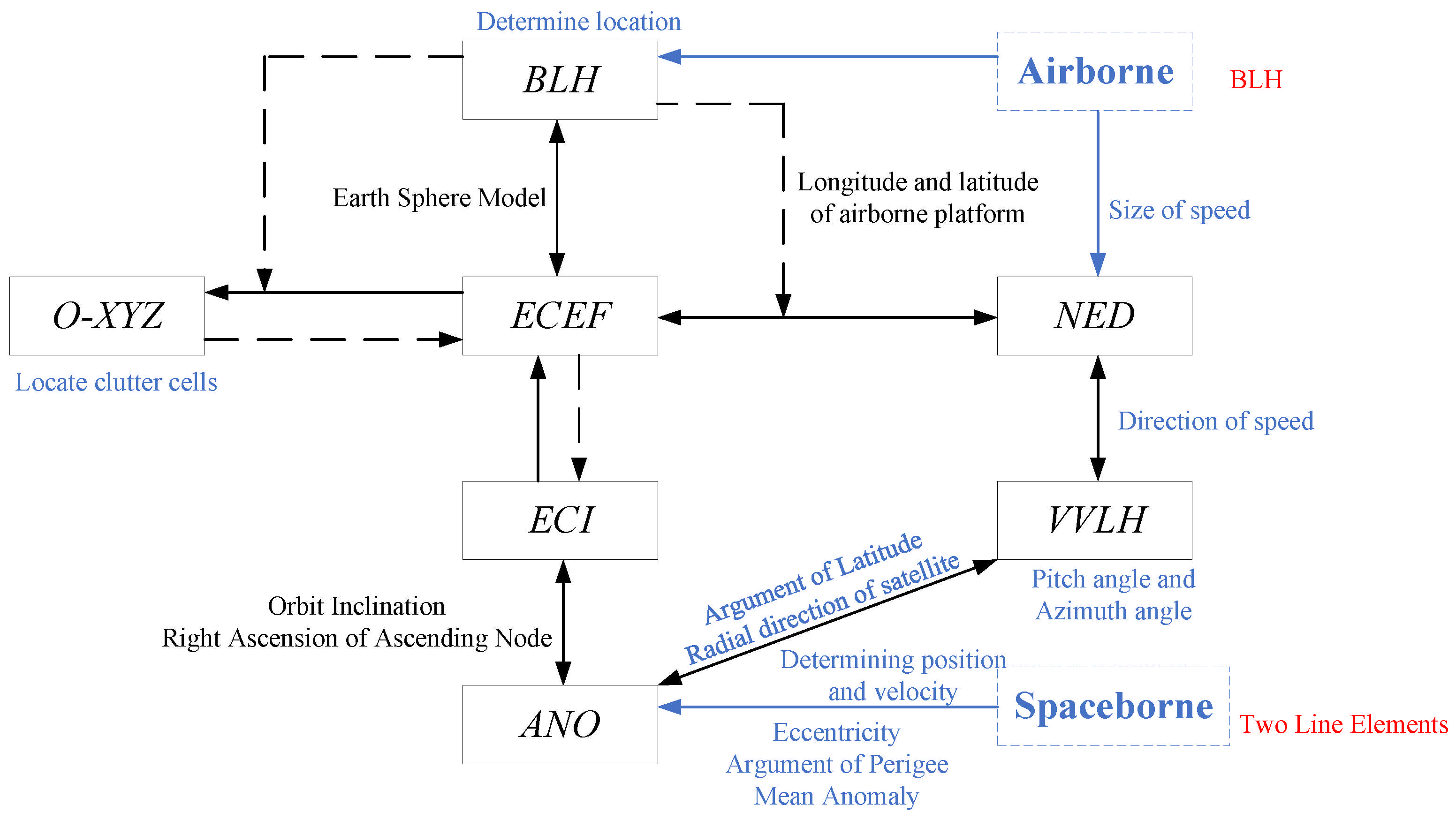
• An SABR clutter signal model for arbitrary geometric configurations is developed based on rigorous coordinate system transformations and satellite-to-Earth geometrical relationships, taking into account the actual radar detection range at the receiver end, as well as the elliptical orbit of the satellite, the curvature of the Earth, and the rotation.
• Based on the proposed model, the non-side-looking receiver clutter characteristics under the geostationary satellite-to-airborne receiver configuration are first analyzed. In conjunction with an evaluation model, the effects of observation areas and geometric configurations on detection performance are investigated using the output signal-to-clutter-noise ratio loss (SCNR_loss) as the performance metric. Finally, recommendations for selecting transceiver geometric configurations and detection areas are presented.

The structure of the paper is outlined as follows: Section 2 presents the signal model of the SABR system, Section 3 analyzes the clutter characteristics across different observation regions, and Section 4 summarizes the research work.

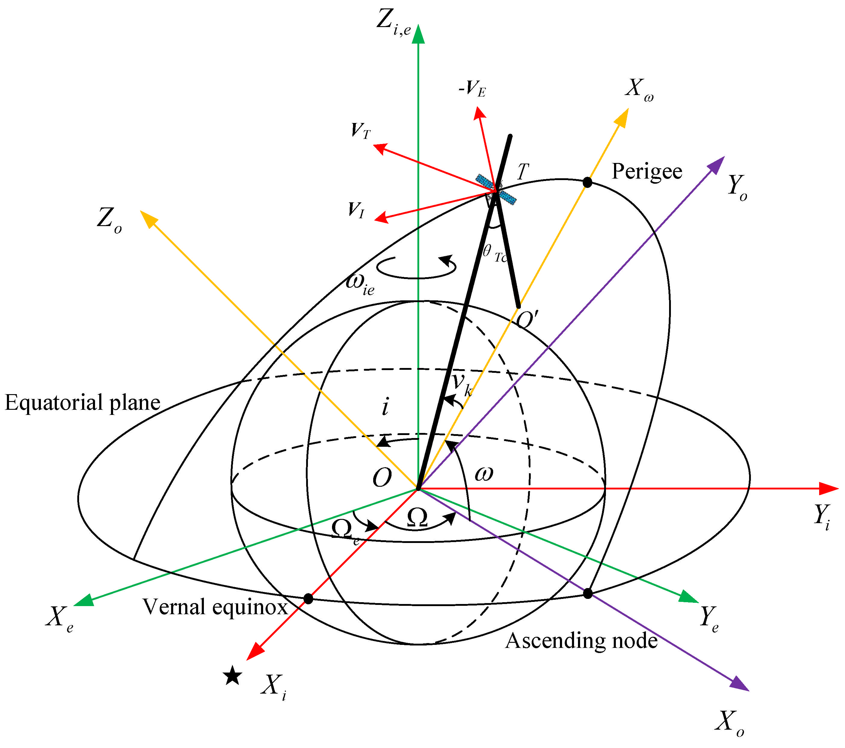
2. Geometrical Configuration and Space-Time Clutter Model for SABR

2.1. Geometrical Configuration of SABR

A representative geometry of an SABR system employing a spaceborne transmitter and an airborne receiver is depicted in Figure 1. The transmitter resides in a satellite orbit, while the receiver (R) is mounted on an airborne platform. The points directly beneath $T^{\prime }$ and $R^{\prime }$ on the Earth’s surface are referred to as their respective sub-satellite points, denoted as H_T and H_R, and represent the respective altitudes of the transmitter and receiver, while v_T and v_R denote their velocity vectors. D means the clutter block at any point with slant distance R_T to the transmitter and R_R to the receiver. The Earth’s center is denoted as O, and its radius is R_e. For analytical simplicity, the Earth is modeled as a perfect sphere in this study.

The iso-range ring of a bistatic radar system is the ellipsoidal ring obtained by intersecting the ground with ellipsoids focusing on the transmitter and receiver. Clutter cells situated on the iso-range rings exhibit identical sum slant distances to the transceiver platforms. In a bistatic radar system, determining iso-range rings on the Earth’s surface is a critical problem. In order to solve this problem, a right-handed coordinate system O-XYZ centered at the Earth’s spherical center O is introduced, facilitating the determination of bistatic clutter iso-range rings under arbitrary configurations by utilizing auxiliary coordinate systems $M\text{-}{X}^{\prime }{Y}^{\prime }{Z}^{\prime }$ and $M\text{-}{X}^{″}{Y}^{″}{Z}^{″}$.

The OZ-axis of the right-handed coordinate system O-XYZ is oriented from the Earth’s center O towards the receiver R. The OX-axis represents the projection of the baseline connecting the transmitter and receiver onto the XOY-plane, while the OY-axis is orthogonal to both the OZ- and OX-axes, following the right-hand rule. The origin O of the coordinate system O-XYZ is translated to point M, followed by a clockwise rotation by an angle $\phi$ about the MY-axis, resulting in the auxiliary coordinate system $M\text{-}{X}^{\prime }{Y}^{\prime }{Z}^{\prime }$. Subsequently, the system is rotated counterclockwise by an angle $\gamma$ about the $M{X}^{\prime }$-axis, yielding the auxiliary coordinate system $M\text{-}{X}^{″}{Y}^{″}{Z}^{″}$, as depicted in Figure 2. The coordinates of the transmitter satellite T are denoted as (T_x, T_y, T_z), and those of the receiver R are denoted as (0, 0, R_z), which represents the elevation angle of the transmitter satellite T relative to the receiver R. $\gamma$ denotes the rotation angle of the ellipse, with T and R serving as its foci. The midpoint of the line segment connecting the transmitter T and the receiver R is represented as M.

Since the clutter is iso-range rings and the clutter unit D (x, y, z) lies on the ring defined by the rotating ellipsoid equation, the height of the transmitting satellite T must exceed that of the receiver R due to the “High-transmit Low-receive” configuration. Therefore, the midpoint coordinates M of the baseline of the receiving and transmitting platform and the angle $\phi$ by which the O-XYZ coordinate system rotates clockwise along the OY axis can be expressed as

$$\left\{\begin{array}{c}M\left({\displaystyle \frac{T_x}{2}},0,{\displaystyle \frac{T_z+R_z}{2}}\right)\hfill \\ \phi =\arctan \left({\displaystyle \frac{T_z-R_z}{2}}\right)\hfill \end{array}\right.$$

(1)

The parameter $\rho$ represents the elliptical centrifugal angle, and the parametric equation for the ellipse corresponding to this clutter cell is provided in (2). The coordinates defined by this equation are expressed in the $M\text{-}{X}^{″}{Y}^{″}{Z}^{″}$-coordinate system.

$$\left\{\begin{array}{c}{x}^{″}=a\cos \rho \hfill \\ y^{″}=b\sin \rho \hfill \\ z^{″}=0\hfill \end{array}\right.$$

(2)

Here, a and b denote the long and short semi-axes of the ellipsoid, respectively. The long semi-axis a equals $R_s/2$, where $R_s$ represents the bi-directional slant distance of the equidistant ring corresponding to the clutter. The short semi-axis b is determined using the geometric relationship $\begin{array}{c}\hfill b=\sqrt{a^2-({(R_x-T_x)}^2+{(R_z-T_z)}^2)/4}\end{array}$.

The transformation from the auxiliary coordinate system $M\text{-}{X}^{″}{Y}^{″}{Z}^{″}$ to the Cartesian coordinate system O-XYZ follows a specific sequence of operations. The process involves an initial clockwise rotation by $\gamma$ around the $M{X}^{″}$ axis to obtain $M\text{-}{X}^{\prime }{Y}^{\prime }{Z}^{\prime }$, followed by a counterclockwise rotation by $\phi$ around the $M{Y}^{\prime }$ axis, and a final translation of the origin from M to O. Consequently, the coordinate transformations can be expressed as

$$\left[\begin{array}{c}x\\ y\\ z\\ 1\end{array}\right]=\mathit{T}\left(-{\displaystyle \frac{T_x}{2}},0,-{\displaystyle \frac{T_z+R_z}{2}}\right){\mathit{T}}_y\left(\phi \right){\mathit{T}}_x\left(-\gamma \right)\left[\begin{array}{c}{x}^{″}\\ y^{″}\\ z^{″}\\ 1\end{array}\right]$$

(3)

where T represents a four-dimensional transformation matrix, incorporating an additional dimension compared to traditional three-dimensional rotation matrices. This additional dimension enables the distinction between positional and velocity information. When the fourth dimension is set to 0, the matrix corresponds to a vector representing velocity. Conversely, when set to 1, it corresponds to a point representing position. Accordingly, the transformation matrix facilitates the representation and differentiation of positional and velocity data in a unified framework. By combining (1), (2), and (3), the following unified result is derived in (4).

$$\left\{\begin{array}{c}x=a\cos \rho \cos \phi -b\sin \rho \sin \gamma \sin \phi +M_x\hfill \\ y=b\sin \rho \cos \gamma \hfill \\ z=a\cos \rho \sin \phi +b\sin \rho \sin \gamma \cos \phi +M_z\hfill \end{array}\right.$$

(4)

where $M_x$ and $M_z$, respectively, denote the x-axis and z-axis values of the midpoint M in the transmitting and receiving platforms, which are $T_x/2$ and $(T_z+R_z)/2$, as shown in (1).

Given that the flight altitude of the airborne platform is negligible compared to the Earth’s radius, the area of clutter detected by the spaceborne-airborne hybrid bistatic radar is only a small fraction of the Earth’s surface. Consequently, ref. [28] employs a planar approximation to simplify the curved surface at the receiver’s sub-satellite point, facilitating the derivation of higher-order nonlinear coupling relations of SABR clutter. As illustrated in Figure 2, the surface beneath the receiver’s sub-satellite point is approximated as the $\delta$-plane The bistatic clutter iso-range ring and the clutter cell D (x, y, z) lie on a rotating ellipsoid. Based on the parametric Equation (4), the equation of the rotating ellipsoid can be derived as (5).

$$\begin{array}{cc}\hfill & {\left(\left(x-M_x\right)\cos \phi +\left(z-M_z\right)\sin \phi \right)}^2/a^2\hfill \\ \hfill & +\left(y^2+{\left(-\left(x-M_x\right)\sin \phi +\left(z-M_z\right)\cos \phi \right)}^2\right)/b^2=1\hfill \end{array}$$

(5)

After the airborne receiving platform ignores the limitation of the Earth’s curvature, the clutter plane $\delta$ can be described as (6).

$$\begin{array}{c}\hfill z=R_{\mathrm{e}}\end{array}$$

(6)

By combining (5) and (6), the generalized expression (7) for the equidistance and ring can be obtained, represented as an ellipse.

$$\begin{array}{c}\hfill {\left(a^2{\sin }^2\phi +b^2{\cos }^2\phi \right)}^2{x}^2+a^2{y}^2+\left(E_1{R}_e+E_2\right)x+E_3{R}_e+E_4+E_5{R}_e^2=0\end{array}$$

(7)

where $E_1$-$E_5$ and ${\mu }_1$-${\mu }_2$ can be denoted, respectively, as (8).

$$\left\{\begin{array}{c}\begin{array}{c}{E}_1=\left(b^2-a^2\right)\sin 2\phi \hfill \\ E_2=2\left(a^2{\mu }_2\sin \phi -b^2{\mu }_1\cos \phi \right)\hfill \\ E_3=-2\left(a^2{\mu }_1\cos \phi +b^2{\mu }_0\sin \phi \right)\hfill \\ E_4=a^2{\mu }_2^2+b^2{\mu }_1^2-a^2{b}^2\hfill \\ E_5=a^2{\cos }^2\phi +b^2{\sin }^2\phi \hfill \\ {\mu }_1=M_x\cos \phi +M_z\sin \phi \hfill \\ {\mu }_2=-M_x\sin \phi +M_z\cos \phi \hfill \end{array}\hfill \end{array}\right.$$

(8)

From the generalized elliptical Equation (7), it is observed that the equation contains only a single x-term. This ellipse can be derived by translating a symmetric elliptical equation, initially centered at the origin, along the x-axis by $\Delta x$. Consequently, (7) can be reformulated into a parameterized elliptical equation in a non-standard form

$$\begin{array}{c}\hfill A{x}^2+B{y}^2+Cx+F=0\end{array}$$

(9)

where A, B, C, F are expressed as follows:

$$\begin{array}{c}\hfill \left\{\begin{array}{c}A=a^2{\sin }^2\phi +b^2{\cos }^2\phi \hfill \\ B=a^2\hfill \\ C=E_1{R}_e+E_2\hfill \\ F=E_3{R}_e+E_4+E_5{R}_e^2\hfill \end{array}\right.\end{array}$$

(10)

By applying the method of completing the square to (9), the standard form of the elliptical equation can be derived as

$$\begin{array}{c}\hfill {\left(\mathrm{x}+\mathrm{C}/2A\right)}^2/\left(\left(C^2-4AF\right)/4A^2\right)+y^2/\left(\left(C^2-4AF\right)/4AB\right)=1\end{array}$$

(11)

Define the major and minor semiaxes of the ellipse as $L_a=(C^2-4AF)/4A^2$ and $L_b=(C^2-4AF)/4AB$, respectively. Therefore, the coordinates of the clutter cell D can be expressed as (12).

$$\begin{array}{c}\hfill \left[\begin{array}{c}x\\ y\\ z\\ 1\end{array}\right]=\left[\begin{array}{c}{L}_a\cos \beta -C/2A\\ L_b\sin \beta \\ R_{\mathit{e}}\\ 1\end{array}\right]\hfill \end{array}$$

(12)

The clutter patch centers are positioned on the bistatic range sum, with the corresponding eccentric angle $\beta \in [0,2\pi ]$ and the azimuth angle constrained by $▵\beta$. To ensure the spatial continuity of the clutter patch, the main lobe beamwidth of the receiver must satisfy the constraint of the azimuthal 3dB beamwidth constraint ${\theta }_R$. In the simulation experiment, the step size of the eccentric angle $\beta$ was appropriately defined as $▵\beta \le 0.9{\theta }_R$. The coordinates of the points on the equidistant sum ring in the O-XYZ coordinate system are calculated by traversing over $\beta$ and substituting the values into (12). Given that the surface at the receiver’s sub-star point is approximated as a plane, the minimum pitch angle ${\theta }_{EL{R}_{\min }}^{\prime }$ derived directly using Earth’s curvature becomes inapplicable for defining the radar’s detection limit. To address this, a modified minimum pitch angle ${\theta }_{EL{R}_{\min }}^{\prime }$ is introduced, as shown in Figure 3, determined by the maximum two-way slant distance $L_{max}$ within the actual detection area. The maximum two-way slant distance $L_{max}$ is located on the side of the line between the transmitter and the receiver, which is far away from the transmitter. The corresponding ${\theta }_{EL{R}_{\min }}^{\prime }$ is calculated by solving a nonlinear equation, ensuring it aligns with the radar’s detection limits at the receiving end. The solution strategy for this nonlinear equation is as follows: The ground distance from the clutter unit to the receiving platform is taken as the unknown quantity x, and the two-way slant range from the ground clutter unit to the transmitting and receiving platform is expressed by the position of the transmitting and receiving platform and the radius of the Earth, and the maximum two-way slant range is subtracted so as to establish a nonlinear equation with only the ground distance x unknown. Then, the right side of the nonlinear equation is set to 0, and the root of the nonlinear function is solved to obtain the ground distance from the clutter unit to the receiving platform corresponding to the maximum two-way slant range; finally, using simple geometric relationships, the pitch angle corresponding to the maximum ground distance of the SABR configuration can be obtained, which is the minimum pitch angle corresponding to the airborne platform under this configuration.

The Earth-Centered Earth-Fixed (ECEF) coordinate system O-X_eY_eZ_e is commonly used as a unified reference frame. The transformation relationship between the right-angle coordinate system $\mathit{O}\text{-}\mathit{XYZ}$ and the O-X_eY_eZ_e system is illustrated in Figure 4. Since the transformation matrix for this relationship is invertible, the matrix from the ECEF system to the $\mathit{O}\text{-}\mathit{XYZ}$ system is first derived. Subsequently, the transformation matrix from $\mathit{O}\text{-}\mathit{XYZ}$ to the ECEF system is obtained by inverting the derived matrix.

The transmitter and receiver positions are defined in the ECEF coordinate system, with the transmitter’s coordinates denoted as ${[x_T,y_T,z_T,1]}^T$ and the receiver’s geodetic coordinates as $({\alpha }_{\mathrm{R}},{\beta }_R,h_R)$, where ${\alpha }_R$, ${\beta }_R$, and $h_R$ represent latitude, longitude, and height, respectively. As shown in Figure 4, the transformation involves two steps. Represented using the transformation matrix based on the homogeneous coordinate system [29], it is as shown in (13) and (15). First, rotation ${\xi }_1$ counterclockwise around the ${\mathit{OZ}}_e$ axis in the $O\text{-}{X}_e{Y}_e{Z}_e$ coordinate system so that ${\mathit{OX}}_e$ is aligned with ${\mathit{OX}}_1$ and ${\mathit{OY}}_e$ is aligned with ${\mathit{OY}}_1$. Then, rotation ${\xi }_2$ counterclockwise around $O{Y}^{″}$ to achieve the conversion from O-X_eY_eZ_e to $O\text{-}{X}^{″}{Y}^{″}{Z}^{″}$.

$$\begin{array}{c}\hfill \left[\begin{array}{c}{X}^{″}\\ Y^{″}\\ Z^{″}\\ 1\end{array}\right]={\mathit{T}}_y\left({\xi }_2\right){\mathit{T}}_z\left({\xi }_1\right)\left[\begin{array}{c}{X}_e\\ Y_e\\ Z_e\\ 1\end{array}\right]={\mathit{T}}_1•\left[\begin{array}{c}{X}_e\\ Y_e\\ Z_e\\ 1\end{array}\right]\end{array}$$

(13)

where ${\xi }_1={\beta }_R$, ${\xi }_2=\pi /2-{\alpha }_R$. Therefore, the coordinates of the transmitter T in the $O\text{-}{X}^{″}{Y}^{″}{Z}^{″}$ coordinate system ${[x_T^{″},y_T^{″},z_T^{″},1]}^{\mathrm{T}}=T_1{[x_{\mathrm{T}},y_{\mathrm{T}},z_{\mathrm{T}},1]}^{\mathrm{T}}$, can be found as (14).

$$\begin{array}{c}\hfill {\xi }_3=\arctan \left(y_T^{″}/x_T^{″}\right).\end{array}$$

(14)

The $O\text{-}{X}^{″}{Y}^{″}{Z}^{″}$ coordinate system is obtained by rotating ${\xi }_3$ counterclockwise around the $O{Z}^{″}$ axis to obtain the O-XYZ coordinate system, so the transformation matrix from O-X_eY_eZ_e to O-XYZ is

$$\begin{array}{c}\hfill \mathit{Tran}={\mathit{T}}_z\left({\xi }_3\right)•{\mathit{T}}_1={\mathit{T}}_z\left({\xi }_3\right)•{\mathit{T}}_y\left(\pi /2-{\alpha }_R\right){\mathit{T}}_z\left({\beta }_R\right).\end{array}$$

(15)

The transformation matrix ${\mathit{Tran}}_{\mathrm{inv}}$ for the O-XYZ coordinate system to ECEF coordinate system is obtained by inverting the transformation matrix $\mathit{Tran}$ of (15).

Moreover, the O-XYZ coordinate system is not suitable for calculating the azimuth and pitch angles. Therefore, a further coordinate transformation is necessary to map the clutter block coordinate system to a coordinate system more appropriate for these calculations. The SABR coordinate system conversion relationship is illustrated in Figure 5.

The following coordinate systems are used: North East Down (NED), Vehicle Velocity Local Horizontal (VVLH), Ascending Node Orbital (ANO), Earth-Centered Inertial Equatorial (ECI), Earth-Centered Earth Fixed (ECEF), and BLH (Longitude, Latitude, and Altitude). The satellite position is calculated using the orbital barycenter and the satellite orbit algorithm from [30], without considering projectile motion. The calculation is divided into two steps. First, the position and velocity of the satellite are calculated in the ascending node orbital coordinate system. Then, they are transformed into the ECEF system using the transformation matrix.

2.2. Transmit Doppler Frequency of SABR

The satellite is assumed to follow a general elliptical orbit around the Earth, as illustrated in Figure 6. In this orbit, ${\mathit{v}}_k$, $\omega$, and $\mathsf{\Omega }$ represent the true anomaly, perigee amplitude angle, and the right ascension of the ascending node, respectively. The parameter i means the orbital inclination and ${\mathsf{\Omega }}_e$ is the angle between the vernal equinox and the zero meridian. Taking into account the curvature and rotation of the Earth, the Doppler frequency shift of the clutter is derived using the velocity vector form. The Doppler frequency of space-based platforms is typically composed of the platform motion and the Earth’s rotation. The velocity vector resulting from the Earth’s rotation on the ground clutter block depends on the position vector of the clutter block. For simplicity, the Earth is treated as stationary, and its rotational velocity is transferred to the satellite [31]. Consequently, the additional velocity vector induced by the Earth’s rotation on the satellite is denoted by ${\mathit{v}}_E^e={\mathsf{\omega }}_e\times {\mathsf{\rho }}_T^e$, where ${\mathsf{\omega }}_{\mathrm{e}}={[0,0,{\omega }_{\mathrm{e}}]}^T$ represents the angular velocity vector of Earth’s rotation, ${\omega }_e=7.292749\times {10}^{-5}\mathrm{rad}/\mathrm{s}$ denotes the Earth’s rotation angular velocity, and ${\mathsf{\rho }}_T^e$ is the position vector of the transmitter T in the O-X_eY_eZ_e coordinate system.

The velocity vector of the satellite in the ECI can be expressed as

$$\begin{array}{c}\hfill {\mathit{v}}_I^e={\mathit{v}}_{Ie}\left({\mathit{u}}_{I{O}^{\prime }}^e\times {\mathit{z}}_o^e\right)\end{array}$$

(16)

where $v_{I_e}=\sqrt{G(2/(H_T+R_e)-1/\mathit{a})}$ represents the magnitude of the satellite’s inertial velocity, G is the gravitational constant of the Earth, and a denotes the semi-major axis of the elliptical orbit. The ${\mathit{u}}_{T{O}^{\prime }}^e\times {\mathit{z}}_o^e$ denotes the unit vector in the direction of the $\mathrm{satellite}’\mathrm{s}$ inertial velocity, where ${\mathit{u}}_{T{O}^{\prime }}^e$ stands for the unit vector in the orbital plane perpendicular to the direction of the satellite’s inertial velocity ${\mathit{v}}_I^e$. ${\theta }_{TC}=arctan\left(sin\left({\mathit{v}}_k\right)/\left(1+ecos\left({\mathit{v}}_k\right)\right)\right)$ is the angle between $T{O}^{\prime }$ and TO, with e representing the eccentricity. And the ${\mathit{u}}_{T{O}^{\prime }}^e$ can be expressed as

$$\begin{array}{c}\hfill {\mathit{u}}_{T{O}^{\prime }}^e=\left[\begin{array}{ccc}\cos {\theta }_{Tc}& -\sin {\theta }_{Tc}& 0\\ \sin {\theta }_{Tc}& \cos {\theta }_{Tc}& 0\\ 0& 0& 1\end{array}\right]{\mathit{u}}_{TO}^e\end{array}$$

(17)

where ${\mathit{u}}_{TO}^e=\left({\mathsf{\rho }}_T^e-{\mathsf{\rho }}_O^e\right)/∥{\mathsf{\rho }}_T^e-{\mathsf{\rho }}_O^e∥$ represents the unit vector from the $\mathrm{Earth}’\mathrm{s}$ spherical center O to the transmitter T in the O-X_eY_eZ_e coordinate system and ${\mathsf{\rho }}_0^{\mathrm{e}}$ denotes the position vector of the Earth’s spherical center O in the O-X_eY_eZ_e coordinate system. ${\mathit{z}}_0^e$ represents the unit vector along the $Z_O$ axis in the O-X_eY_eZ_e coordinate system. The coordinates of ${\mathit{z}}_0^e$ in the O-X_eY_eZ_e system can be determined as (18) using the transformation relationship between the O-X₀Y₀Z₀ and O-X_eY_eZ_e coordinate systems.

$$\begin{array}{cc}\hfill {\mathit{z}}_0^e& =\left[\begin{array}{ccc}\cos \left({\mathsf{\Omega }}_e+\mathsf{\Omega }\right)& -\sin \left({\mathsf{\Omega }}_e+\mathsf{\Omega }\right)& 0\\ \sin \left({\mathsf{\Omega }}_e+\mathsf{\Omega }\right)& \cos \left({\mathsf{\Omega }}_e+\mathsf{\Omega }\right)& 0\\ 0& 0& 1\end{array}\right]\hfill \\ \hfill & \left[\begin{array}{ccc}1& 0& 0\\ 0& \cos i& -\sin i\\ 0& \sin i& \cos i\end{array}\right]\left[\begin{array}{ccc}\cos ({\mathit{v}}_k+\omega )& -\sin ({\mathit{v}}_k+\omega )& 0\\ \sin ({\mathit{v}}_k+\omega )& \cos ({\mathit{v}}_k+\omega )& 0\\ 0& 0& 1\end{array}\right]\left[\begin{array}{c}0\\ 0\\ 1\end{array}\right]\hfill \end{array}$$

(18)

Then, the Doppler frequency of the ground clutter cell D affected by the emission can be expressed as

$$\begin{array}{c}\hfill f_{dT}=\left({\mathit{v}}_T^e•{\mathit{u}}_{TD}^e\right)/\lambda =\left(\left({\mathit{v}}_I^e-{\mathit{v}}_E^e\right)•{\mathit{u}}_{TD}^e\right)/\lambda \end{array}$$

(19)

where $\lambda$ denotes the wavelength, ${\mathit{u}}_{TD}^e=\left({\mathsf{\rho }}_T^e-{\mathsf{\rho }}_D^e\right)/∥{\mathsf{\rho }}_T^e-{\mathsf{\rho }}_D^e∥$ represents the unit vector from the ground clutter block D to the transmitter T, and  ${\mathsf{\rho }}_D^{\mathrm{e}}$ denotes the clutter block D position vector in the O-X_eY_eZ_e coordinate system.

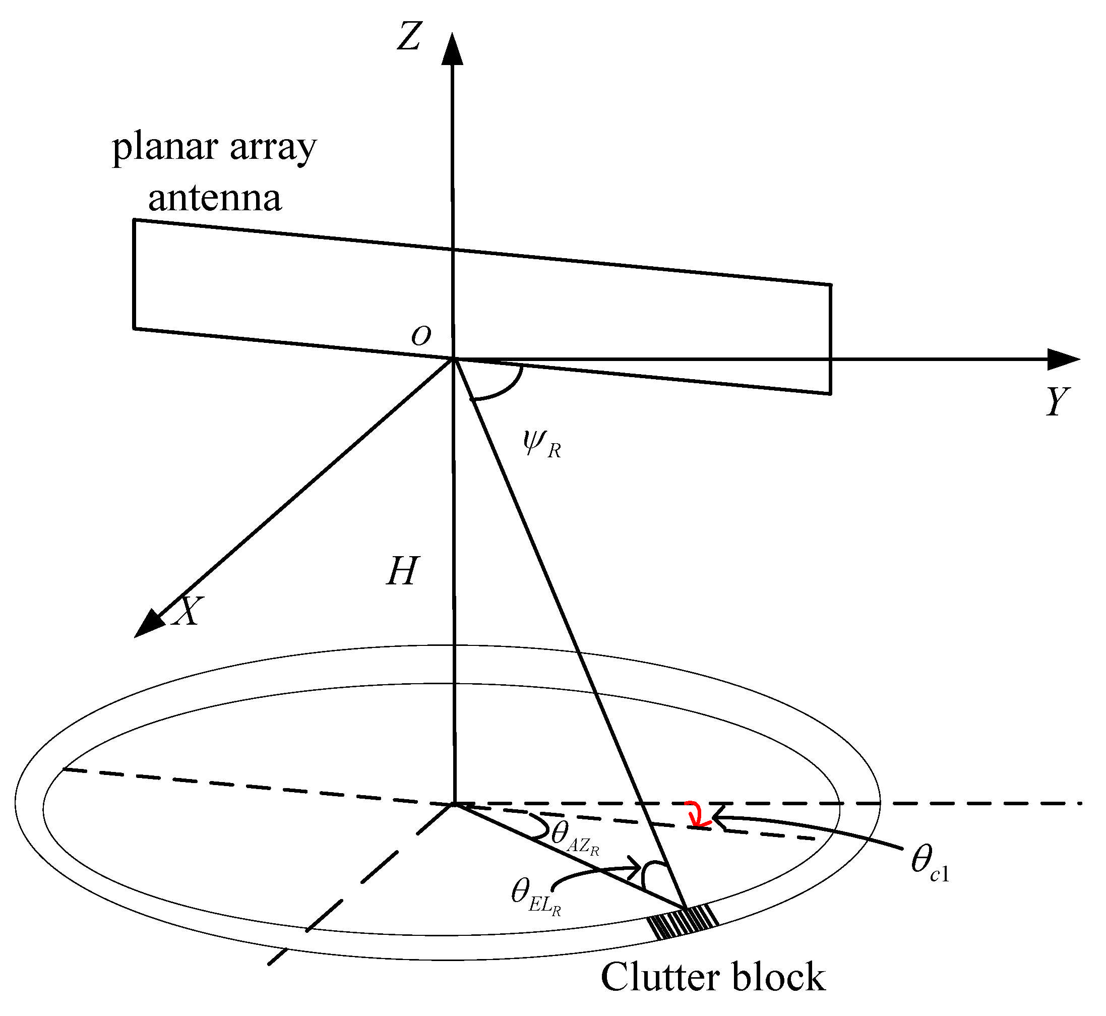
2.3. Receive Doppler Frequency and Spatial Frequency of SABR

Without loss of generality, the receiving antenna array is assumed to be synthesized in columns and uniformly divided into N spatial subarrays along the azimuthal dimension. In the O-XYZ coordinate system, the unit vector $\mathit{u}={\left[\begin{array}{cccc}1& 0& 0& 1\end{array}\right]}^T$ along the X-axis. The homogeneous transformation matrix ${\mathit{Tran}}_{inv}$ from the O-XYZ coordinate system to the ECEF coordinate system is the inverse matrix of (15). Therefore, ${\mathit{u}}_e={\mathit{Tran}}_{inv}\times \mathit{u}$. The spatial frequency of the ground clutter block D is then expressed as

$$\begin{array}{c}\hfill f_s=\left(d/\lambda \right){\mathit{u}}_e·{\mathit{u}}_{RD}^e\end{array}$$

(20)

where d is the array spacing. Formula ${\mathit{u}}_{RD}^e=\left({\mathsf{\rho }}_R^e-{\mathsf{\rho }}_D^e\right)/∥{\mathsf{\rho }}_R^e-{\mathsf{\rho }}_D^e∥$ denotes the unit vector in the direction from the clutter block D to the receiver R, and ${\mathsf{\rho }}_R^e$ denotes the position vector of the receiver R in the O-X_eY_eZ_e coordinate system.

Similarly, the receiver’s velocity vector component in the O-XYZ coordinate system is denoted as v_p. The actual flight scenario introduces an additional velocity vector v_a to the receiver due to unstable airflow and other environmental conditions. From (15), the receiver’s velocity vector components in the O-X_eY_eZ_e coordinate system are obtained as ${\mathit{v}}_p^e$ and ${\mathit{v}}_a^e$. The actual velocity vector of the receiver is then expressed as ${\mathit{v}}_R^e={\mathit{v}}_p^e-{\mathit{v}}_a^e$, and the Doppler frequency at the receiver’s end for the ground clutter unit is expressed as (21)

$$\begin{array}{c}\hfill f_{dR}=\left({\mathit{v}}_R^e·{\mathit{u}}_{RD}^e\right)/\lambda =\left(\left(\left({\mathit{v}}_p^e-{\mathit{v}}_a^e\right)·{\mathit{u}}_{RD}^e\right)/\lambda \right).\end{array}$$

(21)

The fluctuation in the airflow causes a yaw angle between the actual flight direction of the receiver and the intended direction. Combining (19) and (21) yields the Doppler frequency of the ground clutter as

$$\begin{array}{c}\hfill f_d=f_{dT}+f_{dR}.\end{array}$$

(22)

2.4. Clutter Signal Model

Considering that the number of receiving channels is N and K pulses are emitted during the coherent processing interval, the sampling data of the k-th pulse of the n-th way column subarray for the l-th distance ring clutter under ideal conditions, with the noise term neglected, can be expressed as

$$\begin{array}{c}\hfill c_l\left(n,k\right)=\sum _{i=1}^{N_c}{A}_i\exp \left(j\left(n-1\right){\omega }_{si}+j\left(k-1\right){\omega }_{ti}\right)\end{array}$$

(23)

where n = 1, 2,…, N, k = 1, 2, …, K, and l= 1, 2, …, L. N_c denotes the number of clutter blocks in the equidistant ring. In addition, ${\omega }_{si}=2\pi f_{si}$, ${\omega }_{ti}=2\pi f_{di}/f_r$, and A_i represent the normalized spatial frequency, Doppler frequency, and echo signal amplitude of the i-th clutter block, respectively.

Superimposing the received echo signals into an NK-dimensional spacetime snapshot, the l-th equidistant and ring clutter signal model can be represented as (24).

$$\begin{array}{cc}\hfill {\mathit{c}}_l=& {\left[c_l\left(1,1\right),c_l\left(1,2\right),\dots ,c_l\left(1,K\right),c_l\left(2,1\right),\dots ,c_l\left(N,K\right)\right]}^T\hfill \\ \hfill =& \sum _{i=1}^{N_c}{A}_i{\mathit{s}}_s\left(f_{si}\right)\otimes {\mathit{s}}_t\left(f_{di}\right)=\sum _{i=1}^{N_c}{A}_i{\mathit{s}}_i\hfill \end{array}$$

(24)

where s_i represents the space-time vector of the echo signal. As shown in (25), ${\mathit{s}}_s\left(f_{si}\right)$ and ${\mathit{s}}_t\left(f_{di}\right)$ denote the spatial steering vectors and temporal steering vectors of the echo signal, respectively.

$$\begin{array}{c}\hfill {\mathit{s}}_s\left(f_{si}\right)={\left[\begin{array}{cccc}1& \exp \left(j{\omega }_{si}\right)& \cdots & \exp \left(j{\omega }_{si}(N-1)\right)\end{array}\right]}^T\\ \hfill {\mathit{s}}_t\left(f_{si}\right)={\left[\begin{array}{cccc}1& \exp \left(j{\omega }_{ti}\right)& \cdots & \exp \left(j{\omega }_{ti}(K-1)\right)\end{array}\right]}^T\end{array}$$

(25)

The echo signal corresponding to the l-th distance and ring can be expressed as (26).

$$\begin{array}{c}\hfill {\mathit{x}}_l={\mathit{c}}_l+{\mathit{n}}_l\end{array}$$

(26)

where n_l represents the noise component. At this stage, the construction of the echo signal model is complete.

2.5. Clutter Suppression Capability Evaluation Model

The signal-to-clutter-noise ratio loss (SCNR_loss) is defined as the ratio of the output signal-to-clutter-noise ratio (SCNR) of the space-time adaptive filter to that of the space-time matched filter of the ideal environment, which is expressed as

$$\begin{array}{cc}\hfill SCN{R}_{loss}\left({\overline{f}}_d\right)& ={\displaystyle \frac{SCNR\left({\overline{f}}_d\right)}{SN{R}_o}}={\displaystyle \frac{\frac{a^2{\left|{\mathit{W}}^H\left({\overline{f}}_d\right)\mathit{S}\left({\overline{f}}_d\right)\right|}^2}{\left|{\mathit{W}}^H\left({\overline{f}}_d\right)\mathit{R}{\mathit{W}}^H\left({\overline{f}}_d\right)\right|}}{NK\frac{a^2}{{\sigma }^2}}}\hfill \\ \hfill & ={\displaystyle \frac{{\sigma }^2{\left|{\mathit{W}}^H\left({\overline{f}}_d\right)\mathit{S}\left({\overline{f}}_d\right)\right|}^2}{NK\left|{\mathit{W}}^H\left({\overline{f}}_d\right)\mathit{R}{\mathit{W}}^H\left({\overline{f}}_d\right)\right|}}\hfill \end{array}$$

(27)

where N and K represent the number of arrays and pulses, respectively. ${\sigma }^2$ denotes the noise power, and $\mathit{s}\left({\overline{f}}_d\right)$ is the spatial guidance vector corresponding to a Doppler channel when the target’s spatial position is fixed, i.e., always aligned with the direction of the main beam. For the space-time optimal processor, whose clutter covariance matrix R is known, the expression (28) can be obtained by $\mathit{W}={\mathit{R}}^{-1}\mathit{S}\left({\overline{f}}_d\right)$ (27).

$$\begin{array}{c}\hfill SCN{R}_{loss}\left({\overline{f}}_d\right)={\displaystyle \frac{{\sigma }^2}{NK}}\left|{\mathit{S}}^H\left({\overline{f}}_d\right){\mathit{R}}^{-1}\mathit{S}\left({\overline{f}}_d\right)\right|\end{array}$$

(28)

The SCNR loss ranges from 0 to 1, with a larger value indicating better clutter rejection performance of the adaptive filter. In the ideal case of pure noise, the SCNR_loss equals 1, corresponding to 0 dB.

To facilitate a visual comparison of clutter suppression performance, this paper defines the clutter suppression ratio, ${\rho }_1$, as the ratio of the Doppler frequency range where the SCNR loss exceeds 3 dB to the total Doppler frequency range in the SCNR loss vs. the Doppler curve. A smaller value of ${\rho }_1$ indicates better clutter suppression performance.

$$\begin{array}{c}\hfill {\rho }_l={\displaystyle \frac{{\displaystyle \sum _{SCN{R}_{loss}\le -3dB}\overline{f_d}}}{\sum \overline{f_d}}}\end{array}$$

(29)

where $\overline{f_d}$ represents the normalized Doppler frequency curve of SCNR_loss-Doppler.

When evaluating the performance of STAP, the spatial frequency in the target’s space-time steering vector is often fixed, while the Doppler frequency is varied, resulting in a curve of SCNR loss versus Doppler frequency. As the target’s Doppler frequency approaches the clutter frequency, the SCNR loss increases, causing a notch to form near the clutter region. Targets with radial velocities below a certain threshold will fall into this notch, rendering them undetectable. Thus, the Minimum Detectable Velocity (MDV) is defined. Assuming a 5 dB SCNR loss as an acceptable threshold, the target velocity closest to the clutter notch defines the MDV.

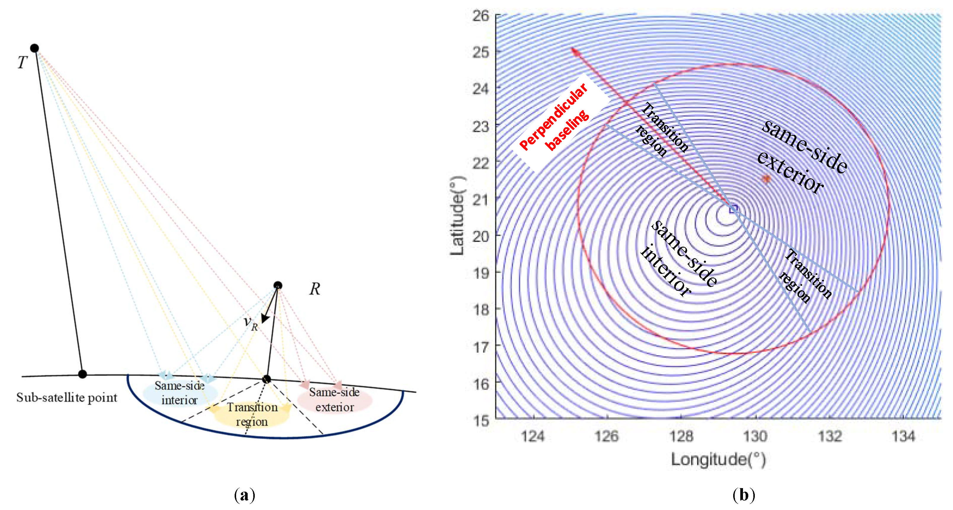
3. Analysis of Clutter Characteristics in Various Observational Regions

The authors of [32] suggest that for the same orbital altitude, forward/backward flight configurations between transceiver satellites typically employ a longer baseline to achieve a larger baseline angle. Consequently, the observation modes for long baselines can be categorized into several types: same front/back view, same inside view, and same outside view. The distance and ring from the lower point of the satellite define the boundary between the inside and outside regions. Furthermore, the division between the front/back and outside regions can be adjusted based on specific requirements. Similarly, the observation region for the “High-transmit Low-receive” configuration can be categorized into the same-side interior region, the same-side exterior region, and a transition region. The dividing line between the same-side interior region and the same-side exterior region is the trajectory of the receiving end when it is flying perpendicularly to the baseline. The transition region represents the intersection of the two regions, where they overlap, as illustrated in Figure 7.

$\alpha$ is the angle between the transceiver platform and the geocentric line. The transmitter is located in a geostationary orbit at (0°N, 111.66°E). The effective detection area of the SABR is primarily determined by the receiver’s coverage area, which is much smaller than that of the transmitter. To clearly illustrate the iso-range ring distributions of the receiver’s detection area, only the receiver’s latitude and longitude (20.7°N, 129.4°E) are shown in Figure 7, marked by blue boxes. The same-side exterior region of the clutter iso-rang ring is more densely distributed on the ground than the same-side interior region. Additionally, the distance ambiguities in the same-side exterior region, at the same distance and ring, are greater than those in the same-side interior region. Therefore, it is evident that the distance ambiguity is strongly dependent on the geometrical configuration of the bistatic, and the number of distance ambiguities varies with the detection angle.

This section analyzes the clutter characteristics and suppression performance in different detection regions based on the signal model developed, under the “High-transmit Low-receive” configuration, with the transmitter in geostationary orbit and the receiver on the airborne platform. The relevant satellite orbit and radar parameters are provided in

Table 1. Orbital parameters.

Parameters	Value (Transmitter/Receiver)
Platform height (HT/HR)	35,786 km/15 km
Orbit inclination (i)	0/–
Right ascension of ascending node ($\mathsf{\Omega }$)	192.71°/–
Argument of periapsis ($\omega$)	251.83°/–
Eccentricity (e)	0/–
True anomaly ($\phi$)	10.76°/–

and

Table 2. Parameters of the radar system.

Parameters	Value and Units
Carrier frequency	1.25 GHz
Bandwidth	1 MHz
Number of pulses in a CPI	256
Channel spacing	0.12
Pulse repetition frequency	2 kHz
Noise figure	2.5 dB
Number of emission channels	668
Number of receive channels	100

.

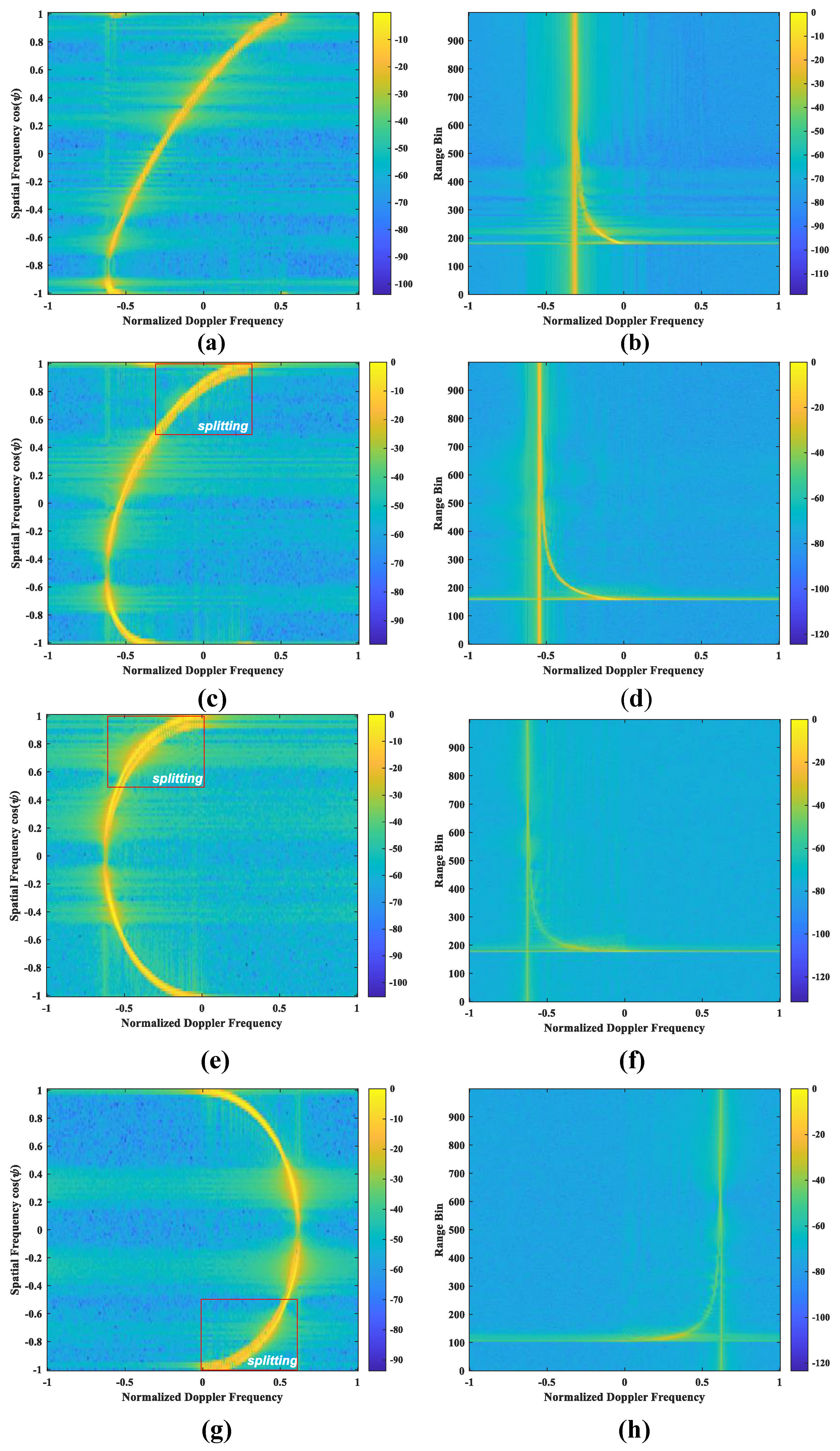
3.1. Clutter Characterization

For non-side-looking radar, the normalized Doppler frequency of the bistatic clutter can be expressed as

$$\begin{array}{c}\hfill {\tilde{f}}_d={\displaystyle \frac{{\nu }_R}{\lambda f_r}}\cos \left({\theta }_{A{Z}_R}+{\theta }_{c1}\right)\cos {\theta }_{E{L}_R}+{\displaystyle \frac{{\nu }_T}{\lambda f_r}}\cos \left({\theta }_{A{Z}_T}+{\theta }_{c2}\right)\cos {\theta }_{E{L}_T}\end{array}$$

(30)

where $\lambda$ and $f_r$ represent the wavelength and pulse repetition frequency, respectively, $v_R$ and $V_T$ represent the velocities of the receiving and transmitting platforms, respectively, ${\theta }_{A{Z}_R}$ and ${\theta }_{A{Z}_T}$ represent the azimuth angles of the receiving and transmitting platforms, respectively, ${\theta }_{E{L}_R}$ and ${\theta }_{E{L}_T}$ represent the elevation angles of the receiving and transmitting platforms, respectively, and ${\theta }_{c1}$ and ${\theta }_{c2}$ represent the yaw angles of the receiving and transmitting platforms, respectively.

Since the transmitter is positioned in a geostationary orbit, v_T = 0 in the ECEF coordinate system, which is substituted into (30).

$$\begin{array}{cc}\hfill {\tilde{f}}_d& ={\displaystyle \frac{{\nu }_R}{\lambda f_r}}\cos \left({\theta }_{A{Z}_R}+{\theta }_{c1}\right)\cos {\theta }_{E{L}_R}\hfill \\ \hfill & ={\displaystyle \frac{{\nu }_R}{\lambda f_r}}\left(\cos {\psi }_R\cos {\theta }_{c1}-\sin {\theta }_{c1}\sqrt{{\cos }^2{\theta }_{E{L}_R}-{\cos }^2{\psi }_R}\right)\hfill \\ \hfill & ={\displaystyle \frac{{\nu }_R}{\lambda f_r}}\left(\cos {\psi }_R\cos {\theta }_{c1}-\sin {\theta }_{c1}\sqrt{\left(R^2-H_R^2\right)/R^2-{\cos }^2{\psi }_R}\right)\hfill \end{array}$$

(31)

As shown in Figure 8, when ${\theta }_{\mathrm{c}1}=0$, i.e., in the case of side-looking radar, the relationship between the two simplifies to

$$\begin{array}{c}\hfill {\tilde{f}}_d={\nu }_R/\left(\lambda f_r\right)\cos {\theta }_{A{Z}_R}\cos {\theta }_{E{L}_R}={\nu }_R/\left(\lambda f_r\right)\cos {\psi }_R\end{array}$$

(32)

Therefore, from (31) and (32), the normalized Doppler frequency of the cluttered block corresponding to the same cone angle for the positive side-view array configuration is independent of distance, while for non-side-looking radar, it varies with distance.

The carrier aircraft generally experiences a yaw angle of 5° to 10° during flight due to factors such as airflow instability. In addition, the air-based receiving platform, which is designed for omnidirectional search, typically has multiple antenna array surfaces, and the angle between these surfaces and the aircraft’s nose is usually non-zero. Therefore, the yaw angle ${\theta }_c$, which results from the combined effect of the platform’s speed direction and the antenna array axis, is defined as the yaw angle. Let the yaw angles be 30°, 60°, 90°, and −90°, where yaw angles of 90° and −90° correspond to Forward-Looking antenna Radar and Backward-Looking antenna Radar, respectively. The main beam is directed towards the clutter cell along the normal to the antenna array plane (i.e., the angle of the main beam is 90°), and the receiving platform’s speed is 150 m/s.

The receiver platform flies along the vertical baseline direction under a non-side-looking radar configuration. Due to the antenna’s suppression of rearward signals, the receiver can only detect signals within the forward half-plane. Consequently, the normalized space-time power spectrum for different yaw angles is shown in Figure 9, along with the corresponding Range-Doppler (RD) power spectra. Specifically, the bistatic range sum for the space-time power spectrum at different yaw angles is consistently 36,816 km, while the slant distances to the receiver are 149.51 km, 173.34 km, and 215.21 km.

As shown in Figure 9, for a non-ideal side-looking antenna array, the normalized Doppler frequency of the clutter block corresponding to the same cone angle varies with distance. In contrast to the space-time power spectra of single-base radar, the space-time power spectra of (a), (c), (e), and (g) exhibit clear spectral splitting due to the strong nonlinear relationship between the Doppler frequency and distance. This results in a significant difference in the Doppler frequencies of the clutter echoes reflected from each range ring, causing the spectral lines to split. From the distance-Doppler power spectra (b), (d), (f), and (h), it is evident that long-range clutter is smeared into the near-range region when distance blurring occurs, leading to a clutter distribution across the entire range and forming a prominent near-range clutter region.

In airborne bistatic radar systems, where the relative velocities of the transmitter and receiver are similar, the time-frequency characteristics of a clutter cell are influenced by both the transmitter and receiver motions. However, in the SABR mode, where the transmitter is positioned on a geostationary satellite, the clutter’s time-frequency characteristics are primarily determined by the receiver’s radial velocity. Consequently, the space-time power spectra and range-Doppler spectra at the receiving end are nearly identical along the baseline, eastward, and vertical flight directions. However, the number of range ambiguities in the observation area varies with the observation angle. This variation is primarily due to the extensive coverage area of the transmitter and the curvature of the Earth, which causes only a portion of the clutter ring echoes to be detected by the receiver.

3.2. Analysis of Clutter Suppression Capability

The airborne receiver platform operates in a positive side-look configuration, with the azimuth beam directed perpendicular to the array. The receiver sequentially flies in the westward direction, 45° west of north (perpendicular to the baseline), 45° east of north (along the baseline), and then eastward. The corresponding SCNR loss curves are shown in Figure 10.

As shown in Figure 10a,b, the red arrow represents the flight direction of the receiver, the ellipse indicates the receiver’s maximum coverage area, and the red asterisk marks the direction of the main beam for the current array configuration. The main beams for the receiver flying toward the west and northwest are located in the same-side exterior region, with 4 and 5 range ambiguities, respectively. In contrast, the main beams for the receiver flying toward the northeast and east are located in the transition region and the same-side interior region, with 3 and 2 range ambiguities, respectively. The analysis shows that the number of range ambiguities is highest when the receiver is flying away from the transmitter and perpendicular to the baseline. It decreases to a minimum of 1 ambiguity as the flight direction approaches the transmitter and aligns perpendicular to the baseline.

As shown in Figure 10c, the receiving platform flies along the directions of due west, northwest, northeast and due east, corresponding to the blue dotted line, red solid line, orange-yellow line and purple solid line in the figure annotation. SCNR loss 3dB corresponds to the blue solid line in the figure. The degree of blurring is higher in the same outer region at the same distance and ring. However, the impact of distance blurring is minimal, as both the yaw angle and the cosine of the cone angle are zero, which also distinguishes this case from the scenario where the SCNR loss curves for the single-base radar are entirely overlapped. In all four cases, the Doppler ranges corresponding to SCNR losses greater than 3 dB represent 11.4% of the total Doppler frequency range.

A comparison of Figure 11a,b reveals that as $\alpha$ decreases, the difference in the number of distance blurs at various angles diminishes, among them, the blue box indicates the location of the receiving platform, and the red "*" symbolizes the direction of the main beam. When $\alpha$ reaches 0°, the number of distance blurs becomes equal at all angles, corresponding to the scenario observed in single-base radar. The pulse repetition frequency primarily determines the maximum unambiguous distance. For a fixed pulse repetition frequency, the distance ambiguity in the same-side interior region is smaller than in the same-side exterior region, and the number of distance ambiguities is most significant along the baseline direction in the same-side exterior region, while the slightest ambiguity in the same-side interior region is along the baseline. Furthermore, the gap in the number of distance ambiguities increases as $\alpha$ increases.

Figure 12 illustrates the variation in SCNR loss with normalized Doppler at different yaw angles, with the receiver flying perpendicular to the baseline, along the baseline, and eastward, respectively. In the non-side-looking radar case, the beam is oriented normally to the array. The blue line indicates the 3 dB SCNR loss level.

Table 3. For different yaw angles and flight directions.

	Yaw 30°	Yaw 60°	Yaw 90°	Yaw −90°
Vertical Baseline/zone	22.6% (same-side exterior)	32.2% (same-side exterior)	42.6% (Transition)	39.6% (Transition)
Along Baseline/zone	21.8% (same-side interior)	22.8% (same-side interior)	38.4% (same-side interior)	41.6% (same-side exterior)
Along East/zone	20.6% (same-side interior)	20.6% (same-side interior)	35.6% (same-side interior)	44.4% (same-side exterior)

shows the ratio ${\rho }_1$, representing the portion of the Doppler frequency range with SCNR loss greater than 3 dB for different yaw angles and flight directions relative to the total Doppler frequency range.

An analysis of the first and second columns of Table 3 reveals that clutter broadening in the same outboard region is more pronounced for identical two-way slant distances and yaw angles. Additionally, the row values in Table 3 indicate that clutter broadening in the forward-view and backward-view arrays is considerably greater than in the antenna slant-view array. Therefore, it is essential to investigate the minimum detectable speed based on SCNR loss for both the forward-looking and backward-looking arrays across different flight directions to inform the selection of the detection area in various flight directions.

As shown in Figure 13, in the backward-looking array, for the three flight scenarios described above, an optimal MDV of 34.54 m/s is achieved when flying along the baseline direction (same as the inboard region), while the worst MDV of 43.65 m/s occurs when flying along the vertical baseline direction (transition area). In the forward-looking array, an optimal MDV of 39.09 m/s is achieved when flying along the vertical baseline direction (transition area), while the worst MDV of 45.57 m/s is observed when flying along the due east direction (same as the outboard region). Therefore, the MDV in the inboard detection region is smaller than in the outboard region. This is because the number of distance blurs in the inboard region is fewer than in the outboard and transition regions, and the clutter broadening caused by distance blurring is less severe.

In summary, reducing the number of distance ambiguities in the airborne receiving platform under the SABR configuration can be achieved through a bistatic geometric configuration. The transmitter and receiver are placed on opposite sides of the detection region, and a larger $\alpha$ angle is selected. This ensures that the detection region is located within the same-side interior region, where the number of distance blurs is smaller. If the detection area is closer to the same-side interior region along the baseline direction, the fewer the distance blurs and the better the minimum detectable velocity (MDV) performance.

4. Conclusions

In this article, an SABR clutter signal model for arbitrary geometric configurations is developed based on rigorous coordinate system transformations and satellite-to-Earth geometrical relationships, taking into account the actual radar detection range at the receiver end, as well as the elliptical orbit of the satellite, the curvature of the Earth, and the rotation. Based on the proposed model, the clutter characteristics of the geostationary synchronous orbit satellite launch-airborne platform receiving configuration are simulated and analyzed. Additionally, in conjunction with the evaluation model, the effects of different observation areas and geometric configurations on performance are evaluated using SCNRLoss as a metric. Recommendations on the geometric configurations of the airborne receiver and the selection of detection areas are provided. Theoretical analysis and simulation results show that:

(1)

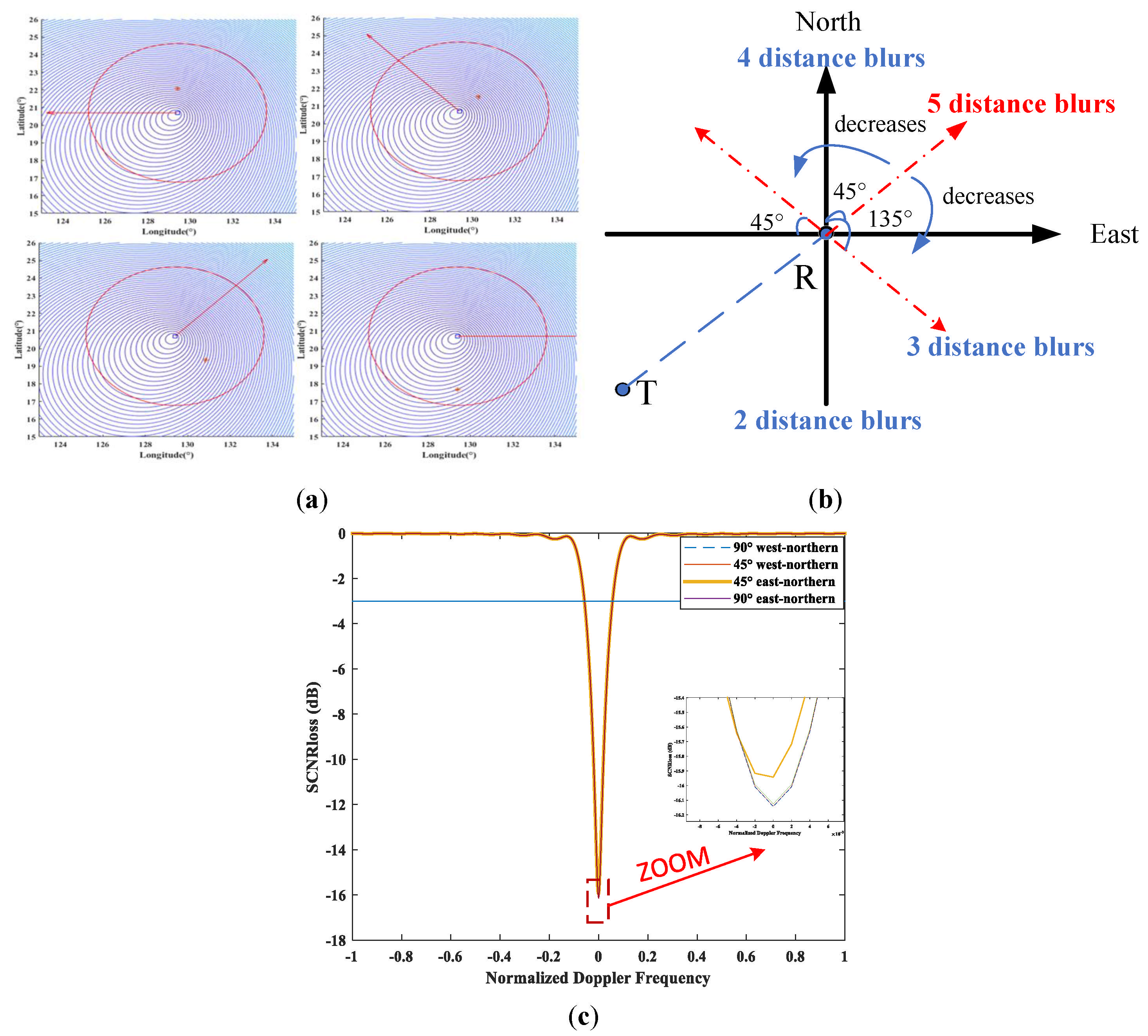
The number of distance blurs is maximal when the receiver is flying perpendicular to the baseline and away from the transmitter, and it reaches a minimum as the flight direction moves closer to the transmitter and vertically toward the baseline.

(2)

In the case of airborne side-looking array reception, although the number of distance blurs is higher in the same-side exterior region at the iso-range ring, the effect of distance blurring is minimal, as both the yaw angle and the cosine of the cone angle are zero. The ${\rho }_{\mathit{l}}$ remains constant at 11.4% across all four cases. The distance blurring is less in the same-side interior region compared to the same-side exterior, with the highest number of distance blurs observed along the baseline direction in the same-side exterior and the lowest in the same-side interior along the baseline direction. Additionally, the gap in the number of distance blurs increases as the $\alpha$ angle increases.

(3)

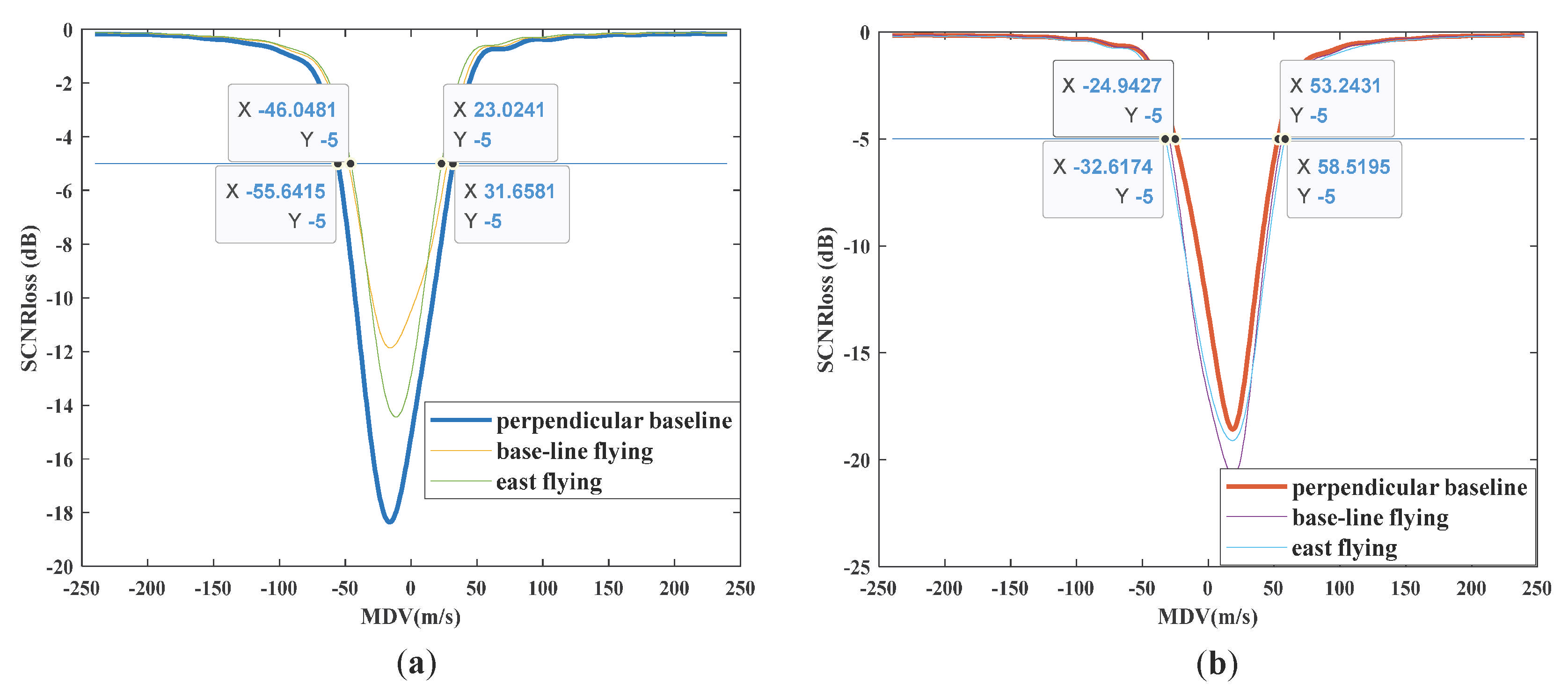
In the case of airborne non-side-looking array reception, the effect of distance blurring leads to significantly greater clutter spread in the front-view and rear-view arrays compared to the antenna slant-view array. As a result, the minimum detectable speed in the outer region (45.57 m/s) is substantially higher than that in the inner region (34.54 m/s).

(4)

To reduce distance ambiguity and improve the minimum detectable speed, these objectives can be achieved through an optimal transceiver geometry configuration. The transmitter and receiver are positioned on opposite sides of the detection area, with a sizeable $\alpha$ angle selected. Additionally, the detection area should be placed as close as possible to the inner region along the baseline direction.

References

1. Hartnett, M.; Davis, M. Operations of an Airborne Bistatic Adjunct to Space Based Radar. In Proceedings of the 2003 IEEE Radar Conference (Cat. No. 03CH37474), Huntsville, AL, USA, 8 May 2003; pp. 133–138. [Google Scholar]
2. Davis, M.; Himed, B.; Zasada, D. Design of Large Space Based Radar for Multimode Surveillance. In Proceedings of the 2003 IEEE Radar Conference (Cat. No. 03CH37474), Huntsville, AL, USA, 8 May 2003; pp. 1–6. [Google Scholar]
3. Hartnett, M.; Davis, M. Bistatic Surveillance Concept of Operations. In Proceedings of the 2001 IEEE Radar Conference (Cat. No. 01CH37200), Atlanta, GA, USA, 3 May 2001; pp. 75–80. [Google Scholar]
4. Hsu, Y.; Lorti, D. Spaceborne Bistatic Radar—An Overview. IEEE Proc. F Commun. Radar Signal Process. 1986, 133, 642–648. [Google Scholar] [CrossRef]
5. Griffiths, H. From a Different Perspective: Principles, Practice and Potential of Bistatic Radar. In Proceedings of the 2003 International Conference on Radar (IEEE Cat. No. 03EX695); Adelaide, SA, Australia, 3–5 September 2003, pp. 1–7.
6. Zhang, Q.; Dong, Z.; Zhang, Y.; He, Z. GEO-UAV Bistatic Circular Synthetic Aperture Radar: Concepts and Technologies. In Proceedings of the 2016 IEEE International Geoscience and Remote Sensing Symposium (IGARSS), Beijing, China, 10–15 July 2016; pp. 4195–4198. [Google Scholar]
7. Guttrich, G.; Sievers, W.; Tomljanovich, N. Wide Area Surveillance Concepts Based on Geosynchronous Illumination and Bistatic Unmanned Airborne Vehicles or Satellite Reception. In Proceedings of the 1997 IEEE National Radar Conference, Syracuse, NY, USA, 13–15 May 1997; pp. 126–131. [Google Scholar]
8. Han, L.; Chen, Z.; Duan, R.; Jiang, C. Modeling of Varying Geometrical Scenarios of Bistatic Radar. In Proceedings of the 2007 International Symposium on Intelligent Signal Processing and Communication Systems, Xiamen, China, 28 November–1 December 2007; pp. 196–199. [Google Scholar]
9. Pillai, U.; Li, K.; Himed, B. Space Based Radar: Theory and Applications; McGraw-Hill: New York, NY, USA, 2008. [Google Scholar]
10. Li, W.; Wang, L.; Liu, D.; Chen, T.; Li, Z.; Wu, J.; Yang, H.; Yang, J. Raw Data Simulation under Undulating Terrain for Bistatic SAR with Arbitrary Configuration. IEEE J. Sel. Top. Appl. Earth Obs. Remote Sens. 2024, 17, 12878–12892. [Google Scholar] [CrossRef]
11. Liu, K.; Wang, T.; Huang, W. An Efficient Sparse Recovery STAP Algorithm for Airborne Bistatic Radars Based on Atomic Selection under the Bayesian Framework. Remote Sens. 2024, 16, 2534. [Google Scholar] [CrossRef]
12. Tan, X.; Yang, Z.; Li, X.; Liu, L.; Li, X. Clutter Rank Estimation Method for Bistatic Radar Systems Based on Prolate Spheroidal Wave Functions. Remote Sens. 2024, 16, 2928. [Google Scholar] [CrossRef]
13. Liu, J.; Liao, G. Spaceborne-Airborne Bistatic Radar Clutter Modeling and Analysis. In Proceedings of the 2011 IEEE CIE International Conference on Radar, Chengdu, China, 24–27 October 2011; Volume 1, pp. 915–918. [Google Scholar]
14. Liu, N.; Zhang, L.; Yi, Y.; Liu, X. Clutter modeling and analysis for spaceborne bistatic radar. In Proceedings of the 2007 IET International Conference on Radar Systems, Edinburgh, UK, 15–18 October 2007; IET: London, UK, 2007; pp. 1–5. [Google Scholar]
15. Li, H.; Tang, J.; Peng, Y. Clutter Modeling and Characteristics Analysis for Bistatic SBR. In Proceedings of the 2007 IEEE Radar Conference, Waltham, MA, USA, 17–20 April 2007; pp. 513–517. [Google Scholar]
16. Zhang, C.; Liu, H.; Long, T. Signal-to-Noise Ratio Analysis in Satellite-Airship Bistatic Space Based Radar. In Proceedings of the 2008 International Conference on Radar, Adelaide, SA, Australia, 2–5 September 2008; pp. 434–439. [Google Scholar]
17. Sun, Z.; Wu, J.; Pei, J.; Li, Z.; Huang, Y.; Yang, J. Inclined Geosynchronous Spaceborne–Airborne Bistatic SAR: Performance Analysis and Mission Design. IEEE Trans. Geosci. Remote Sens. 2016, 54, 343–357. [Google Scholar] [CrossRef]
18. Rodriguez-Cassola, M.; Baumgartner, S.; Krieger, G.; Moreira, A. Bistatic TerraSAR-X/F-SAR Spaceborne–Airborne SAR Experiment: Description, Data Processing, and Results. IEEE Trans. Geosci. Remote Sens. 2010, 48, 781–794. [Google Scholar] [CrossRef]
19. Espeter, T.; Walterscheid, I.; Klare, J.; Ender, J. Synchronization Techniques for the Bistatic Spaceborne/Airborne SAR Experiment with TerraSAR-X and PAMIR. In Proceedings of the 2007 IEEE International Geoscience and Remote Sensing Symposium, Barcelona, Spain, 23–28 July 2007; pp. 2160–2163. [Google Scholar]
20. Wang, W.Q.; Shao, H. Azimuth-Variant Signal Processing in High-Altitude Platform Passive SAR with Spaceborne/Airborne Transmitter. Remote Sens. 2013, 5, 1292–1310. [Google Scholar] [CrossRef]
21. Huang, P.; Zou, Z.; Xia, X.G.; Liu, X.; Liao, G.; Xin, Z. Multichannel Sea Clutter Modeling for Spaceborne Early Warning Radar and Clutter Suppression Performance Analysis. IEEE Trans. Geosci. Remote Sens. 2021, 59, 8349–8366. [Google Scholar] [CrossRef]
22. Li, Z.; Ye, H.; Liu, Z.; Sun, Z.; An, H.; Wu, J.; Yang, J. Bistatic SAR Clutter-Ridge Matched STAP Method for Nonstationary Clutter Suppression. IEEE Trans. Geosci. Remote Sens. 2022, 60, 1–14. [Google Scholar] [CrossRef]
23. Liu, Z.; Ye, H.; Li, Z.; Yang, Q.; Sun, Z.; Wu, J.; Yang, J. Optimally Matched Space-Time Filtering Technique for BFSAR Nonstationary Clutter Suppression. IEEE Trans. Geosci. Remote Sens. 2022, 60, 1–17. [Google Scholar] [CrossRef]
24. Zhang, S.; Gao, Y.; Xing, M.; Guo, R.; Chen, J.; Liu, Y. Ground Moving Target Indication for the Geosynchronous-Low Earth Orbit Bistatic Multichannel SAR System. IEEE J. Sel. Top. Appl. Earth Obs. Remote Sens. 2021, 14, 5072–5090. [Google Scholar] [CrossRef]
25. Zhang, T.; Wang, Z.; Xing, M.; Zhang, S.; Wang, Y. Research on Multi-Domain Dimensionality Reduction Joint Adaptive Processing Method for Range Ambiguous Clutter of FDA-Phase-MIMO Space-Based Early Warning Radar. Remote Sens. 2022, 14, 5536. [Google Scholar] [CrossRef]
26. Wang, Z.; Chen, W.; Zhang, T.; Xing, M.; Wang, Y. Improved Dimension-Reduced Structures of 3D-STAP on Nonstationary Clutter Suppression for Space-Based Early Warning Radar. Remote Sens. 2022, 14, 4011. [Google Scholar] [CrossRef]
27. Li, H.; Tang, J.; Peng, Y. Effects of Geometry on Clutter Characteristics of Hybrid Bistatic Space Based Radar. In Proceedings of the 2006 CIE International Conference on Radar, Shanghai, China, 16–19 October 2006; pp. 1–4. [Google Scholar]
28. Kan, Q.; Xu, J.; Liao, G.; Zhang, Y.; Xu, Y.; Wang, W. Clutter Characteristics Analysis and Range-Dependence Compensation for Space–Air Bistatic Radar. IEEE Trans. Geosci. Remote Sens. 2024, 62, 1–15. [Google Scholar] [CrossRef]
29. Blinn, J.F.; Newell, M.E. Clipping using homogeneous coordinates. In Proceedings of the 5th Annual Conference on Computer Graphics and Interactive Techniques, Atlanta, GA, USA, 23–25 August 1978; pp. 245–251. [Google Scholar]
30. Xie, G. Principles of GPS and Receiver Design; Publishing House of Electronics Industry: Beijing, China, 2009; Volume 7, pp. 61–63. [Google Scholar]
31. Zulch, P.; Davis, M.; Adzima, L.; Hancock, R.; Theis, S. The Earth Rotation Effect on a LEO L-Band GMTI SBR and Mitigation Strategies. In Proceedings of the 2004 IEEE Radar Conference (IEEE Cat. No. 04CH37509), Philadelphia, PA, USA, 29 April 2004; pp. 27–32. [Google Scholar]
32. Tan, X.; Yang, Z.W.; He, P.Y.; Wu, X.Y. Analysis of clutter characteristics and parameters selection for following configuration of spaceborne bistatic radar. Syst. Eng. Electron. 2023, 45, 2735–2743. [Google Scholar]
Figure 1. Geometrical configuration of spaceborne-airborne bistatic radar.
Remotesensing 17 01222 g001
Figure 2. Geometric model approximation of clutter iso-range ring: (a) O-XYZ and auxiliary coordinate systems; (b) The ellipse is translated along the x-axis.
Remotesensing 17 01222 g002
Figure 3. Modified minimum pitch angle.
Remotesensing 17 01222 g003
Figure 4. O - X e Y e Z e  O-XYZ coordinate system.
Remotesensing 17 01222 g004
Figure 5. SABR coordinate system transformation relationship.
Remotesensing 17 01222 g005
Figure 6. Depiction of satellite orbit and satellite velocity components.
Remotesensing 17 01222 g006
Figure 7. “High-transmit Low-receive” observation model ( α  = 27°): (a) geometric diagram; (b) the iso-range ring.
Remotesensing 17 01222 g007
Figure 8. Non-side-looking array geometry of an airborne receiving platform.
Remotesensing 17 01222 g008
Figure 9. The normalized space-time power spectrum and Range-Doppler spectrum spectra correspond to different yaw angles for flight in the vertical baseline direction: (a,b) correspond to a yaw angle of 30°, (c,d) to 60°, (e,f) to 90°, and (g,h) to −90°.
Remotesensing 17 01222 g009
Figure 10. Side-looking west, northwest, northeast and due east, corresponding to the blue dotted line, red solid line, orange-yellow line and purple solid line in the figure annotation. SCNR loss 3dB corresponds to the blue solid line in the figure). radar ( α  = 27°): (a) Iso-rang ring in all flight directions. (b) A schematic of the number of distance blurs in different directions. (c) the SCNR loss curve in side-looking radar.
Remotesensing 17 01222 g010
Figure 11. Equidistant and ring during flight along the due east direction for side-looking radar: (a α  = 27°; (b α  = 1.72°. Among them, the blue box indicates the location of the receiving platform, and the red "*" symbolizes the direction of the main beam.
Remotesensing 17 01222 g011
Figure 12. Comparison of SCNRloss curves for different yaw angles and receiver flight directions: (a) SCNRloss curve for the receiver flight direction perpendicular to the baseline; (b) SCNRloss curve for the receiver flight direction along the baseline; (c) SCNRloss curve for the receiver flight direction along the east.
Remotesensing 17 01222 g012
Figure 13. Comparison of MDV of airborne platforms along different directions in the case of non-side-looking array: (a) backward-looking arrays; (b) forward-looking arrays.
Remotesensing 17 01222 g013