Effects of Emission Variability on Atmospheric CO₂ Concentrations in Mainland China

Abstract

Accurately assessing the impact of anthropogenic carbon dioxide (CO₂) emissions on CO₂ concentrations is essential for understanding regional climate change, particularly in high-emission countries like China. This study employed the GEOS-Chem chemical transport model to simulate and compare the spatiotemporal distributions of XCO₂ of three anthropogenic CO₂ emission inventories in mainland China for the 2018–2020 period and analyzed the effects of emission variations on atmospheric CO₂ concentrations. In eastern China, particularly in the Yangtze River Delta (YRD) and Beijing-Tianjin-Hebei (BTH) regions, column-averaged dry air mole fractions of CO₂ (XCO₂) can exceed 420 ppm during peak periods, with emissions from these areas contributing significantly to the national total. The simulation results were validated by comparing them with OCO-2 satellite observations and ground-based monitoring data, showing that more than 70% of the monitoring stations exhibited a correlation coefficient greater than 0.7 between simulated and observed data. The average bias relative to satellite observations was less than 1 ppm, with the Emissions Database for Global Atmospheric Research (EDGAR) showing the highest degree of agreement with both satellite and ground-based observations. During the study period, anthropogenic CO₂ emissions resulted in an increase in XCO₂ exceeding 10 ppm, particularly in the North China Plain and the YRD. In scenarios where emissions from either the BTH or YRD regions were reduced by 50%, a corresponding decrease of 1 ppm in XCO₂ was observed in the study area and its surrounding regions. These findings underscore the critical role of emission control policies in mitigating the rise in atmospheric CO₂ concentrations in densely populated and industrialized areas. This research elucidates the impacts of variations in anthropogenic emissions on the spatiotemporal distribution of atmospheric CO₂ and emphasizes the need for improved accuracy of CO₂ emission inventories.

1. Introduction

CO₂, as one of the most significant greenhouse gases, plays a crucial role in Earth’s radiative balance and contributes to climate change. The global mean CO₂ mole fraction reached 417.1 ± 0.1 parts per million (ppm) in 2022 [1]. The rising concentration of CO₂ is a major driver of climate change, contributing to global temperature increases [2,3] and exacerbating the frequency and intensity of extreme weather events, including heatwaves, floods, and droughts [4]. Since the Industrial Revolution, the persistent increase in atmospheric CO₂ levels has primarily been attributed to human activities such as fossil fuel combustion, industrial production, and land-use changes. The average annual anthropogenic flux of CO₂ from fossil fuel emissions between 2013 and 2022 was 9.6 Gt C yr⁻¹, with the total carbon emissions reaching 10.9 Gt C yr⁻¹ [5]. Thus, reducing and controlling CO₂ emissions is recognized as a global priority. China accounted for approximately 31% of global fossil fuel CO₂ emissions in 2022 [5], establishing its role as a key contributor in global carbon emissions and climate change. Consequently, accurate quantification of China’s carbon emissions is essential to achieve global emission reduction targets and implement effective climate policies.

However, substantial uncertainties remain in carbon emission inventories. These uncertainties primarily stem from discrepancies in energy consumption statistics, emission factor estimates, land-use change data, and spatiotemporal inconsistencies in regional data [6,7,8,9]. Global CO₂ emission estimates are accurate to within ±6.5%, while the range of uncertainties for country-level total CO₂ emissions is between ±4% and ±35% [10]. Solazzo et al. reported that the uncertainty in anthropogenic emissions of the three main greenhouse gases—carbon dioxide (CO₂), methane (CH₄), and nitrous oxide (N₂O)—in the EDGAR inventory ranged from 15% to 20% in 2015 [11]. Previous studies indicated that average uncertainties are below ±5% in developed countries [9,12], while in developing countries, uncertainties range from ±10% to ±50% [1,12,13,14,15]. As a developing country with a vast territory, China faces significant challenges in emission inventory accuracy due to substantial errors in activity-level statistics and substantial regional disparities in emission factors caused by uneven economic development [16]. These factors contribute to higher levels of uncertainty in emission inventories compared to developed nations. For China, reported anthropogenic emissions vary by over 10% across different statistical sources [16,17,18], primarily due to regional energy-use inconsistencies and the complexity of land-use changes. At sub-national scales, such as provinces, cities, or large point sources, accurately capturing CO₂ emissions from fossil fuels and other anthropogenic sources is hindered by factors including economic competition and regional disparities in energy sourcing [19]. Given the scale and uncertainty of China’s carbon emissions, precise quantification of these emissions is crucial for developing effective reduction strategies.

Chemical transport models (CTMs) are essential tools that link emissions and concentrations. CTMs are widely used to improve the accuracy of CO₂ flux estimates and refine model simulations by comparing model outputs with observational data. Common CTMs include the Goddard Earth Observing System 3-D chemical transport model (GEOS-Chem), the Weather Research and Forecasting (WRF) model coupled with Chemistry (WRF-Chem), and the Community Multiscale Air Quality (CMAQ) [20]. These models are driven by meteorological fields and incorporate atmospheric chemistry, physical processes, and various emission inventories to simulate the spatial and temporal variations in CO₂ concentrations. Satellite observations offer distinct advantages for model evaluation and optimization. Satellites such as the Orbiting Carbon Observatory-2 (OCO-2) [21], Greenhouse Gases Observing Satellite (GOSAT) [22], and the Chinese Carbon Dioxide Observation Satellite (TanSat) [23] provide high spatiotemporal resolution global XCO₂ data, helping to address the spatial coverage limitations of ground-based observations. For instance, OCO-2 captures XCO₂ with spatial resolution better than 3 km, providing critical data for identifying localized emission hotspots in urban and industrial areas.

Additionally, ground-based observation networks such as the Total Carbon Column Observing Network (TCCON) [24] and Collaborative Carbon Column Observing Network (COCCON) [25] provide high-precision XCO₂ measurements using infrared spectrometers, serving as essential benchmarks for validating model simulations. Comparative analyses of simulations and observations frequently reveal systematic biases between simulated and observed data [26,27,28,29]. These discrepancies may arise from inaccuracies in emission inventories, incomplete chemical mechanisms in models, or inaccuracies in atmospheric dynamics. Ma et al. [30] utilized the WRF-STILT atmospheric transport model to simulate CO₂ concentrations in the Yangtze River Delta of China and performed Bayesian inversion using tower-based CO₂ observations to estimate anthropogenic CO₂ fluxes. Numerous studies have explored the impact of changes in prior carbon fluxes on simulated CO₂ outcomes, indicating that alterations in oceanic carbon fluxes and biomass burning emission inventories can substantially affect CO₂ concentration patterns [8,31,32]. Assimilation techniques, such as four-dimensional variational assimilation (4D-Var) [33] and Ensemble Kalman Filter (EnKF) [34,35], are employed to enhance the accuracy of emission inventories. This approach, which integrates observational data with models, provides critical insights into regional carbon emissions and the global carbon cycle. It also promotes improvements in emission inventories and strengthens the application of atmospheric chemistry models.

This study aims to quantitatively assess the impact of anthropogenic emission inventories and their uncertainties on the forward simulation of atmospheric CO₂ concentrations. Anthropogenic CO₂ emissions constitute a substantial portion of global carbon sources. This study conducted a consistency analysis between simulation results based on three different anthropogenic CO₂ emission inventories and both satellite and ground-based observational data. The findings may serve as a reference for selecting emission inventories in forward simulations and inversions. Additionally, they provide information on the distribution of biases between CO₂ simulation results and observational data, which can support the optimization process of these inventories in the inversion framework. To achieve this goal, we conducted nested simulations of CO₂ concentrations over East Asia from 2018 to 2020 using the GEOS-Chem and three distinct anthropogenic CO₂ emission inventories. Based on these simulations, we designed a series of numerical experiments to evaluate the impact of emission level variations. We evaluated the sensitivity of atmospheric CO₂ concentrations to variations in anthropogenic emission fluxes using OCO-2 observations and ground-based measurements. The remainder of this paper is organized as follows: Section 2 details the models, data, and methodologies used in this study; Section 3 provides a comparative analysis of emission inventories and validates simulations against OCO-2, TCCON, and NOAA-ESRL ground observations. The conclusions and significance of this research are summarized in Section 4.

2. Materials and Methods

2.1. Model Description

The Goddard Earth Observing System 3-D chemical transport model (GEOS-Chem) is developed and maintained by the Goddard Earth Observing System (GEOS) of Global Modeling and Assimilation Office (GMAO). GEOS-Chem is capable of simulating atmospheric composition at both global and regional scales. The initial CO₂ simulation in GEOS-Chem was introduced by Suntharalingam et al. [36], and significant updates were made later by Nassar et al. [37], particularly in terms of improving the sources of prior carbon fluxes.

A nested simulation of CO₂ concentrations over the East Asian region was conducted from 1 January 2018 to 1 January 2021 using the GEOS-Chem model. The initial CO₂ concentration fields were obtained from Carbon Tracker (CT2022). First, a global simulation was performed with a horizontal resolution of 2° latitude × 2.5° longitude and 47 vertical layers to simulate the global spatial and temporal distribution of CO₂. The results of this global simulation were then used as boundary conditions for a nested simulation over the East Asian region at a finer resolution of 0.5° latitude × 0.625° longitude. The GEOS-Chem model is driven by meteorological data and emission flux data. In this study, the Modern-Era Retrospective analysis for Research and Applications (MERRA-2) was used for the meteorological inputs. The specific input CO₂ flux data used in the simulations are detailed as follows, (1) The fossil fuel combustion emission inventories used in this study include three anthropogenic emission inventories: the Open-source Data Inventory for Anthropogenic CO₂ (ODIAC) [38], the Multi-resolution Emission Inventory for China (MEIC) [39,40], and the Emissions Database for Global Atmospheric Research (EDGAR) [10]. (2) The biomass burning inventory is derived from the Global Fire Emissions Database, Version 4.1s (GFEDv4.1s) [41], with a spatial resolution of 0.25° × 0.25°. (3) Ocean exchange flux is scaled monthly ocean exchange with interannual variation [42], with a spatial resolution of 4° × 5°. (4) The balanced biosphere exchange flux is represented by the Simple Biosphere Model (SiB3) [43], with a temporal resolution of 3 h. The annual total of the balanced biosphere exchange flux is zero, but it is used to simulate the carbon cycle within a single day. (5) The net terrestrial exchange data are derived from the TransCom climatology dataset [44], representing a fixed terrestrial net ecosystem exchange flux. (6) Shipping and aviation emissions are provided by the Community Emissions Data System (CEDS) [45] and the Aviation Emissions Inventory Code (AEIC) [46,47].

This study focuses on anthropogenic CO₂ emission inventories. Therefore, three major emission inventories were selected for the simulations: ODIAC, EDGAR, and MEIC. With all other input data and parameters kept constant, the anthropogenic CO₂ emission inventory was substituted with one of the three inventories in each case, resulting in three corresponding CO₂ spatiotemporal distribution simulation outcomes (hereafter referred to as sim_ODIAC, sim_EDGAR, and sim_MEIC). It was assumed that any differences in simulation results were solely due to variations in the anthropogenic emission inventories, enabling an analysis of the impact of anthropogenic emissions on simulated atmospheric CO₂ concentrations. Additionally, a “no_fossil” experiment was conducted in which fossil fuel emissions were completely turned off in the model setup. The differences between the “no_fossil” experiment and other simulations were attributed exclusively to anthropogenic emissions during the study period [7,48]. Based on this setup, a series of numerical experiments were further conducted by adjusting the initial emission amounts proportionally.

2.2. Emissions

This study utilized three widely used anthropogenic CO₂ emission inventories, namely, ODIAC, MEIC, and EDGAR, to investigate their impact on CO₂ simulations. These three inventories were consistently adjusted to 1° × 1° monthly emission datasets for use as input data for the model.

2.2.1. ODIAC

ODIAC is a global, high-resolution CO₂ emission dataset developed by the National Institute for Environmental Studies (NIES). This study utilized the ODIAC2022 dataset at a 1° × 1° monthly resolution [49]. The ODIAC dataset derives national CO₂ emissions for each country based on global combustion statistics from the British Petroleum (BP) Statistical Review of World Energy [50]. The spatial distribution of CO₂ emissions is enhanced using point source data from CARMA and nighttime lights observations [38]. Nighttime lights data closely correlate with the distribution of human settlements and land transportation areas. The uncertainties in the ODIAC emission inventory arise from three primary sources: (i) uncertainties in national and regional emission estimates; (ii) incomplete global power plant coverage in Carbon Monitoring and Action (CARMA), leading to emissions inferred from incomplete data [51]; and (iii) the assumption that nighttime lights data directly correspond to CO₂ emissions, which is often less reliable in developing countries [52].

2.2.2. MEIC

MEIC is a comprehensive database of anthropogenic pollutant and greenhouse gas emissions developed and managed by Tsinghua University [39,40]. MEIC has been widely used in research fields, including air pollution control and air quality assessments. The activity levels in MEIC are based on provincial statistical data, with emission factors derived from existing measurements within China. Emissions are initially allocated at the county level using statistical indicators such as GDP, population, and agricultural activities. Subsequently, additional gridded data, such as population density and transportation networks, are employed as spatial proxies to further distribute emissions within grid cells. However, limitations in the available underlying data introduce uncertainty into the emission estimates. MEIC currently provides multi-sectoral CO₂ emission data at a resolution of 0.25° × 0.25° for the period from 1990 to 2020.

2.2.3. EDGAR

EDGAR is a global anthropogenic emission dataset developed by the European Commission’s Joint Research Centre (JRC) [10]. Emissions in EDGAR are calculated using IPCC accounting methodologies, with activity-level data derived primarily from international datasets such as those provided by the International Energy Agency (IEA) and BP statistical data. The emissions are spatially distributed to a 0.1° × 0.1° grid using spatial proxies including population density, transportation data, power plant locations, and agricultural land use maps [53].

2.3. Satellite Observations

The OCO-2 satellite, launched in 2014, is designed to deliver high-precision atmospheric CO₂ observations. The three-channel imaging spectrometer onboard OCO-2 measures solar radiation in the near-infrared and shortwave infrared regions, specifically at 760 nm (O₂-A band), 1610 nm (weak CO₂ absorption band), and 2060 nm (strong CO₂ absorption band). OCO-2 operates in a sun-synchronous orbit at an altitude of 705 km, crossing the equator at approximately 13:36 local time. With a spatial resolution of 1.29 × 2.25 km, OCO-2’s high spatial resolution and accuracy make it particularly suitable for monitoring CO₂ concentration variations at regional scales [54,55]. In this study, we utilized the bias-corrected OCO-2_L2_Lite_FP_V10 product [56], which has been rigorously quality-controlled and bias-corrected to exclude unreliable data. To ensure the reliability of the results, only measurements with a Quality Flag of 0 were used.

OCO-2_L2_Lite_FP_V10 product provides XCO₂, whereas the GEOS-Chem simulation provides CO₂ concentration profiles across 47 layers. To compare the model simulations with satellite data, the simulated results were adjusted using averaging kernels and prior profiles to derive the modeled CO₂ concentrations at the corresponding spatiotemporal locations. The specific calculation is given by the following formula [57]:

$$XC{O}_2^m=XC{O}_2^a+{\displaystyle \sum _j}{h}_j{a}_j{\left(y_m-y_a\right)}_j$$

(1)

where $XC{O}_2^a$ represents the prior XCO₂ from OCO-2, j denotes the atmospheric layers, $h_j$ is the pressure-weighted function of the j-th layer, $a$ is the column averaging kernel, and $y_m$ and $y_a$ represent the modeled and prior CO₂ vertical profiles, respectively. The parameters such as $XC{O}_2^a$, $y_a$, and $a_j$ were obtained from the OCO-2_L2_Lite_FP_V10 product.

2.4. Ground-Based CO₂ Observations

To validate the reliability of the model simulation results, ground-based observations from the Total Carbon Column Observing Network (TCCON), along with surface CO₂ concentration observations provided by the Observation Package (ObsPack) product (obspack_co2_1_GLOBALVIEWplus_v9.1) from the Carbon Cycle and Greenhouse Gases (CCGG) Global Greenhouse Gas Reference Network measurement program, were used. TCCON employs Fourier Transform Infrared Spectrometers (FTIR) to record solar absorption spectra in the near-infrared range, from which column-averaged dry air mole fractions of gases such as CO₂, CH₄, and N₂O are derived [24,58]. The latest TCCON dataset (GGG2020) used in this study achieves high measurement accuracy, with XCO₂ errors below 0.6 ppm when the solar zenith angle is less than 82° [59]. Due to its high observational accuracy, TCCON data are extensively used for analyzing greenhouse gas concentration distributions and validating satellite products [54]. For this study, XCO₂ observations from four TCCON stations [60,61,62,63] in East Asia were selected for subsequent analysis. Surface CO₂ observation data were obtained from ObsPack product distributed by the Global Monitoring Laboratory of Earth System Research Laboratories (NOAA-ESRL) [64]. The ObsPack product is derived from in situ measurements or flask air samples; its reliability has been validated in previous studies [8,29,65]. Accordingly, surface CO₂ concentration data from seven locations in China and surrounding East Asian regions were selected to evaluate GEOS-Chem’s simulation of CO₂ concentrations.

The Taylor Diagram was utilized in this study to assess the performance of GEOS-Chem in simulating CO₂ concentrations. A Taylor Diagram [66] is a polar coordinate plot commonly applied in meteorology and environmental science to evaluate and quantify the similarity between one or more simulated fields and observed data. The Taylor Diagram incorporates three key metrics: the correlation coefficient (R), the centered root mean square error (RMSE-c), and the standard deviations ratio (std_r). It is defined as follows:

$$R={\displaystyle \frac{1}{N}}{\displaystyle \sum _{i=1}^N}[(x_{mi}-\overline{x_m})(x_{oi}-\overline{x_o})]/({\sigma }_m{\sigma }_o)$$

(2)

$$RMSE-c=\sqrt{{\displaystyle \frac{1}{N}}{\displaystyle \sum _{i=1}^N}{[(x_{mi}-\overline{x_m})-(x_{oi}-\overline{x_o})]}^2}$$

(3)

$$std\_r={\displaystyle \frac{{\sigma }_m}{{\sigma }_o}}$$

(4)

$${\sigma }_m=\sqrt{{\displaystyle \frac{1}{N}}{\displaystyle \sum _{i=1}^N}{(x_{mi}-\overline{x_m})}^2}$$

(5)

$${\sigma }_o=\sqrt{{\displaystyle \frac{1}{N}}{\displaystyle \sum _{i=1}^N}{(x_{oi}-\overline{x_o})}^2}$$

(6)

where $\overline{x_m}$ and $\overline{x_o}$ represent the mean values of the model and observation data, respectively; $N$ refers to all the data from a specific site involved in the calculation; and ${\sigma }_m$ and ${\sigma }_o$ represent the standard deviations of the simulated and observation data, respectively. These three metrics are represented concurrently within the diagram and are interrelated through a cosine relationship. Specifically, the reference point (REF) on the diagram represents the observed values. The angle between the simulated and observed values represents the correlation coefficient, the distance between the model point and the reference point represents RMSE-c, and the radial distance from the origin to the model point indicates the deviation ratio of the observed and simulated values. A higher R value, a lower RMSE-c, and a standard deviation ratio closer to 1 indicate better model performance. In other words, the closer the simulation point is to the REF point, the more accurate the simulation results.

3. Results and Discussion

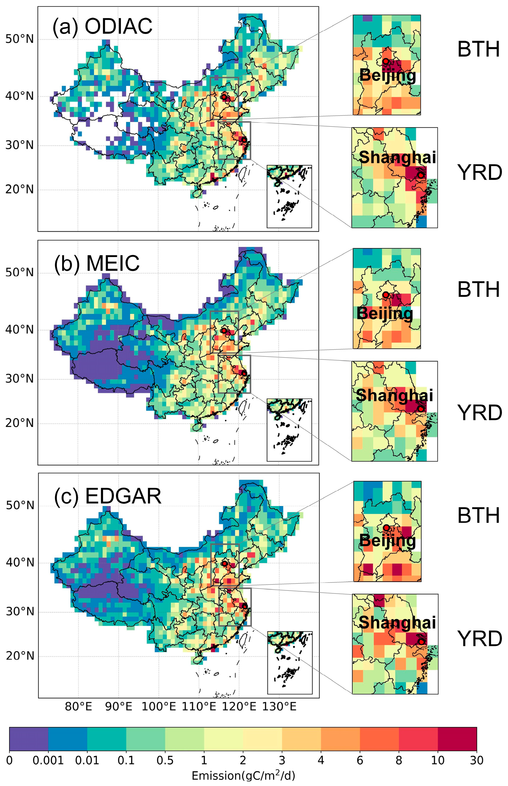
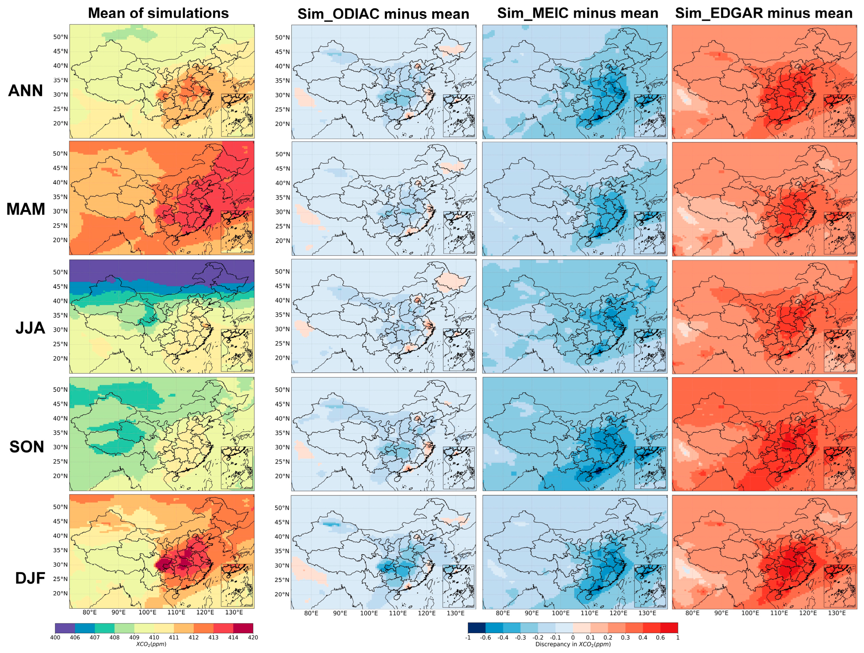
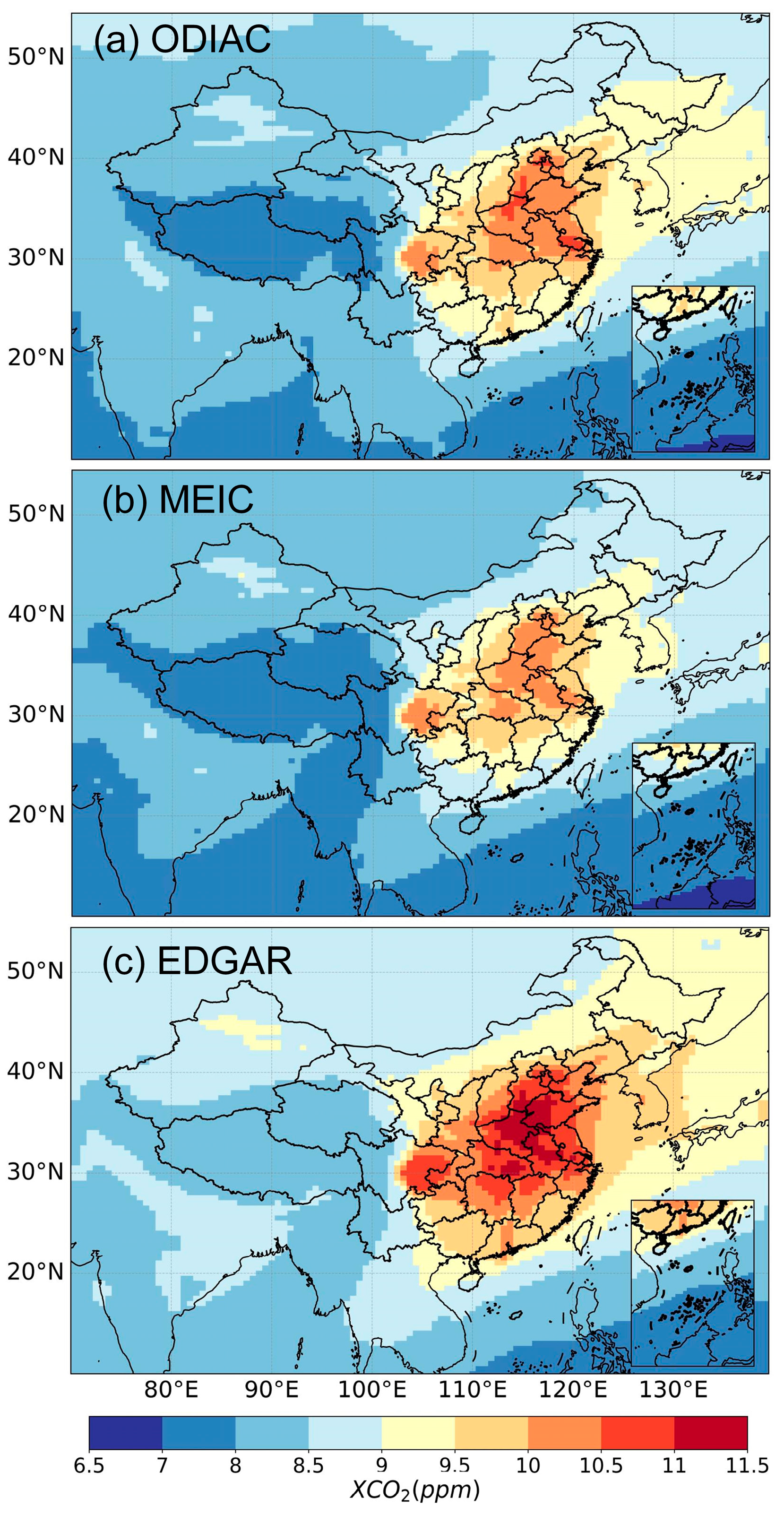
3.1. Spatiotemporal Distribution of Emissions and Simulated XCO₂

Figure 1 presents the daily mean CO₂ emissions from 2018 to 2020 based on the ODIAC, MEIC, and EDGAR emission inventories, with units expressed in gC/m²/day. The resolution of all three emission inventories has been unified to 1° × 1°. The blank areas in the mainland China region of the figure represent areas where emission values are zero in the inventories due to data gaps or sparsely populated regions. Regarding the overall spatial distribution of emissions, all three emission inventories consistently show a pattern of higher emissions in eastern China and lower emissions in the western regions. Low emissions are primarily observed in the economically underdeveloped northwestern regions of China, including Qinghai, Tibet, and southeastern Xinjiang, due to sparse human activity. In contrast, areas with high anthropogenic emissions are predominantly concentrated in the eastern and coastal regions, notably within economically developed urban agglomerations like BTH and YRD. These regions are characterized by high populations densities, rapid economic growth, and substantial fossil fuel consumption, resulting in considerable anthropogenic CO₂ emissions. The differences in emissions across the three inventories are primarily observed in the emission hotspots and regional distributions. Compared to the other two inventories, ODIAC shows significantly higher emission levels in Beijing, Shanghai, and surrounding cities. Emissions in these areas reach up to 10 gC/m²/day. The MEIC inventory displays slightly lower emissions in the southern coastal cities compared to the other two inventories. The EDGAR inventory reveals more emission hotspots with CO₂ emissions exceeding 8 gC/m²/day. However, the local emission peak in Beijing and its surrounding areas is slightly lower than that in the other two inventories.

All three inventories exhibited noticeable variability in monthly anthropogenic CO₂ emissions in mainland China from 2018 to 2020 (Figure 2), with emissions being generally higher in winter and lower in summer. This seasonal trend is likely associated with increased heating demand and the seasonal variations in energy consumption during winter. The three inventories demonstrated strong consistency in their temporal trends, with most monthly CO₂ emissions fluctuating between 0.7 and 1.1 Gt. Moreover, a significant decline in CO₂ emissions was observed in early 2020 due to the outbreak of the COVID-19 pandemic, which led to a substantial reduction in economic activities. As economic activities gradually resumed, emissions showed a recovery trend across all inventories. Notably, the EDGAR inventory consistently reported higher overall emission levels compared to ODIAC and MEIC, a finding that aligns with previous studies [53]. In terms of fluctuation characteristics, the MEIC inventory exhibited more pronounced variability compared to ODIAC and EDGAR. For instance, emissions of MEIC inventory in February 2020 dropped sharply, amounting to only half of the emissions recorded in the preceding two months. This heightened sensitivity may be attributed to the MEIC inventory’s reliance on detailed local data for statistical inputs and emission factors, making it more responsive to regional emission changes. These differences likely reflect variations in the statistical methodologies and source accounting approaches among the inventories. They collectively reveal the seasonal variations in anthropogenic CO₂ emissions in mainland China and underscore the influence of economic activities on emission levels.

The annual distribution of XCO₂ across East Asia exhibited a clear spatial pattern, with higher concentrations in the eastern regions and lower concentrations in the western regions, as shown in Figure 3. Higher XCO₂ were mainly observed in the southeastern and central regions of China, where the average concentrations during 2018–2020 exceeded 411 ppm. Eastern regions of China, characterized by high population density, advanced industrial activities, and economic development, generated substantial CO₂ emissions. In contrast, western and northeastern China displayed lower XCO₂ levels due to sparser populations, lower industrial activity, and extensive forest coverage in the northeast, where active vegetation absorption leads to lower XCO₂ levels. These findings were consistent with previous CO₂ simulations and observations [65,67,68]. In spring (MAM), XCO₂ concentrations increased markedly, especially in eastern and northern China, reaching over 413 ppm. During summer (JJA), XCO₂ was generally lower, falling below 409 ppm, reflecting the absorption effects of vegetation. In autumn (SON), XCO₂ levels rose again across East Asia, particularly along eastern coastal areas of China. XCO₂ peaked during winter (DJF), especially in central and eastern China, with values reaching up to 420 ppm. This pattern underscores the significant influence of heating and industrial emissions during this season. Furthermore, significant differences were observed among the simulation results of the ODIAC, MEIC, and EDGAR inventories (Figure 3). The simulation results from the ODIAC inventory showed minimal differences from the mean, with most regions exhibiting slightly lower values than the average for all three inventories. However, in high-emission cities such as Beijing, Shanghai, and Guangzhou, as well as their surrounding areas, the simulated values were slightly higher than the mean. The simulation results from the MEIC inventory were lower than the mean, particularly in the eastern coastal regions of China. The simulated XCO₂ of EDGAR was the highest, with significant differences primarily concentrated in southeastern China and adjacent coastal areas, reaching up to 0.4–1 ppm. Moreover, seasonal variations in these differences were more pronounced, with the EDGAR simulation showing greater XCO₂ deviations from the mean during the SON and DJF. Overall, the differences among the three inventories were mainly reflected in the spatial distribution and intensity of emissions in high-emission areas.

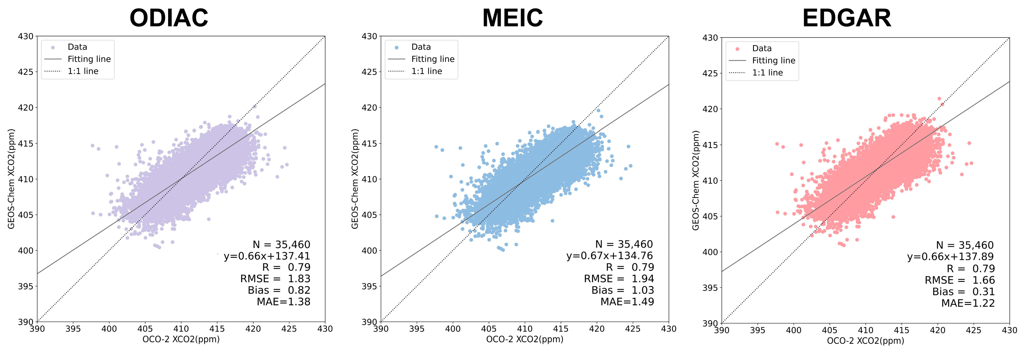
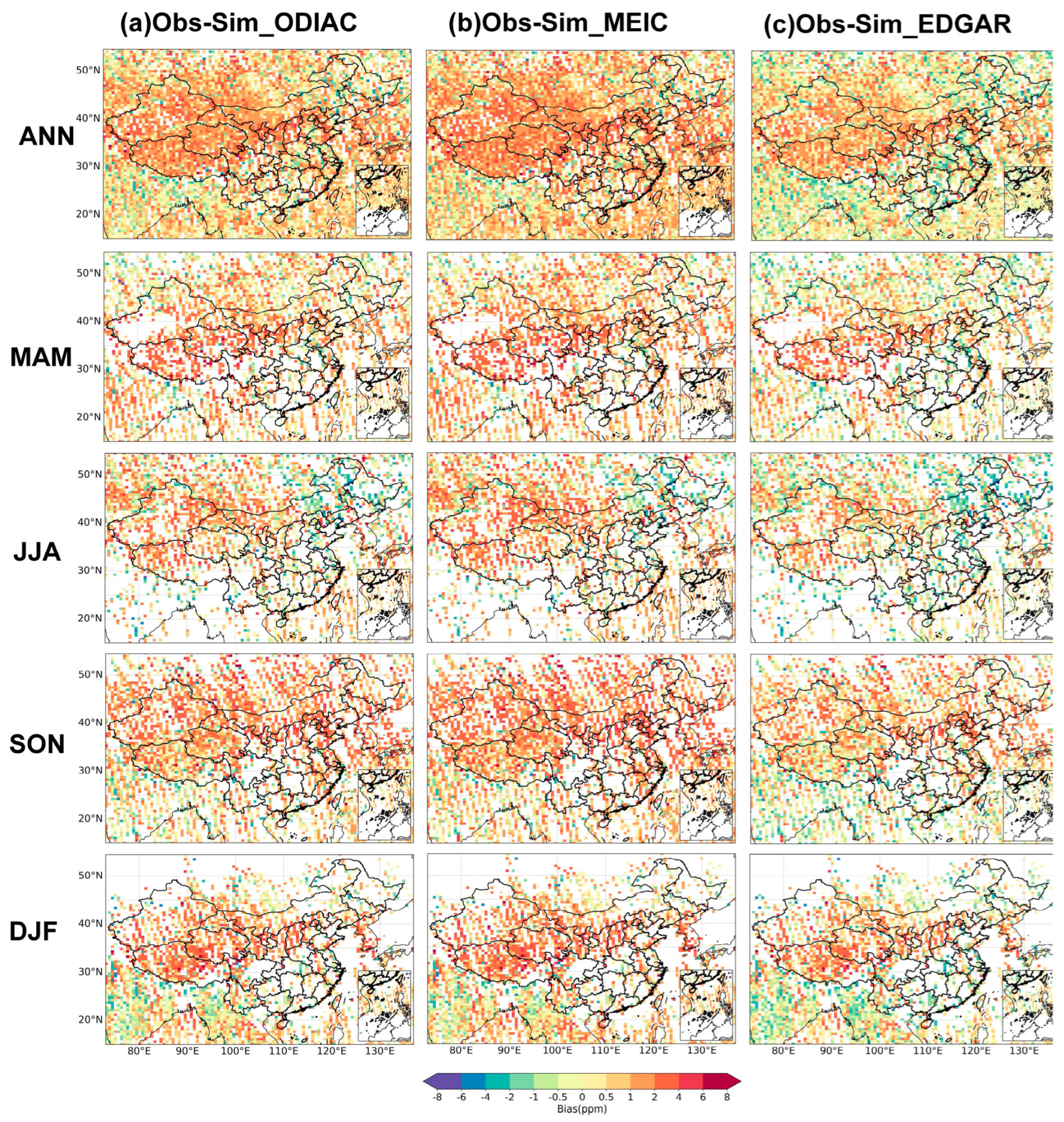
3.2. Comparisons with Satellite XCO₂

To validate the accuracy of simulated XCO₂, OCO-2 observations in 2020 were compared with the corresponding simulated XCO₂. On an annual scale, the simulations based on the three emission inventories exhibited a correlation coefficient of 0.79 with OCO-2 observations (Figure A1), with biases (XCO₂_OCO minus XCO₂_Sim) ranging from 0.31 to 1.03 ppm. Among the inventories, the simulations using the EDGAR inventory showed the smallest discrepancy when compared with OCO-2 XCO₂ observations (Figure A1). Figure 4 illustrates the bias between OCO-2 XCO₂ and GEOS-Chem simulated XCO₂ at the corresponding spatiotemporal locations for the year 2020 and across each season. On an annual scale, OCO-2 XCO₂ generally exhibited a positive bias (Bias > 0) relative to the GEOS-Chem simulations, with biases primarily ranging from −1 to 4 ppm. The discrepancies were particularly pronounced in western and northern China, where satellite retrievals tended to overestimate XCO₂ [29]. This overestimation was mainly attributed to high aerosol concentrations and elevated surface albedo in the northwestern desert regions, which increased retrieval errors and led to localized overestimation. In MAM, the most significant biases were observed in central China. During JJA, the biases of all three inventories were relatively small, ranging mainly from −1 to 1 ppm and showing a more uniform spatial distribution. In some parts of northeastern China, simulated XCO₂ exceeded satellite observations, likely due to uncertainties in the terrestrial biosphere effects that caused model overestimation during JJA [7]. In SON, the biases of ODIAC and MEIC were more pronounced, with biases reaching up to 6 ppm, suggesting possible inaccuracies in emission estimates in these areas. In contrast, the EDGAR inventory exhibited lower biases compared to the other two inventories. During DJF, high biases were predominantly concentrated in western China, with EDGAR showing biases within the range of −1 to 1 ppm in other regions.

The deviations between the simulated results from the three emission inventories and satellite-observed XCO₂ were analyzed across different seasons (

Table 1. Statistical parameters between OCO-2 observations and simulations in 2020.

		Mean of XCO2 (ppm)	The Mean of Highest 10% XCO2 (ppm)	The Mean of Lowest 10% XCO2 (ppm)	Bias (ppm)	MAE (ppm)	RMSE (ppm)	Correlation Coefficient
MAM	Obs_OCO-2	414.50	417.51	411.51
	Sim_ODIAC	413.79	415.88	411.81	0.72	1.22	1.66	0.52
	Sim_EDGAR	414.26	416.39	412.24	0.24	1.09	1.51	0.52
	Sim_MEIC	413.61	415.67	411.65	0.89	1.30	1.74	0.52
JJA	Obs_OCO-2	410.73	415.40	404.80
	Sim_ODIAC	410.06	413.73	405.29	0.67	1.42	1.86	0.83
	Sim_EDGAR	410.59	414.26	405.82	0.14	1.29	1.74	0.83
	Sim_MEIC	409.84	413.54	405.01	0.88	1.51	1.93	0.83
SON	Obs_OCO-2	411.45	415.18	407.88
	Sim_ODIAC	410.32	412.68	407.97	1.13	1.54	1.99	0.60
	Sim_EDGAR	410.88	413.56	408.53	0.56	1.28	1.73	0.60
	Sim_MEIC	410.06	412.35	407.70	1.39	1.70	2.15	0.60
DJF	Obs_OCO-2	413.04	416.71	410.38
	Sim_ODIAC	412.32	414.86	410.38	0.72	1.36	1.82	0.53
	Sim_EDGAR	412.80	415.58	410.74	0.25	1.24	1.68	0.55
	Sim_MEIC	412.11	414.54	410.21	0.93	1.45	1.91	0.53

). Overall, XCO₂ over mainland China was lowest in JJA, with an average of 410.73 ppm observed by OCO-2, and higher in DJF and MAM, at 414.50 ppm and 413.04 ppm, respectively. The bias between the model simulations and observations ranged from 0.15 to 1.39 ppm, with RMSE values below 2.15 ppm, indicating the reliability of the simulations. It is noteworthy that the seasonal mean biases (XCO₂_OCO minus XCO₂_Sim) were generally positive, suggesting that the models tended to underestimate XCO₂ to some extent. This underestimation may be largely attributed to uncertainties in other types of carbon fluxes included in the simulation [65].We calculated and analyzed the annual global CO₂ flux estimates from the Global Carbon Project (

Table A1. Global CO₂ flux estimated by Global Carbon Project (GCP) for the 2018–2020 period (unit: GtC yr⁻¹) and all uncertainties are reported as ±1δ.

	2018	2019	2020
Fossil CO2 emissions	10 + 0.5	9.7 ± 0.5	9.3 ± 0.5
Land-use change emissions	1.5 ± 0.7	1.8 ± 0.7	0.9 ± 0.7
Total emissions	11.5 ± 0.9	11.5 ± 0.9	10.2 ± 0.8
Partitioning
Ocean sink	2.6 ± 0.6	2.6 ± 0.6	3.0 ± 0.4
Terrestrial sink	3.5 ± 0.7	3.1 ± 1.2	2.9 ± 1.0
Annual CO2 fluxes	5.4	5.8	4.3
Reference	[71]	[72]	[73]

), as well as the CO₂ flux datasets used in this study (

Table A2. Summary of inventories for GEOS-Chem CO₂ simulations in this work along with global annual CO₂ flux during the study period (2018–2020) (unit: GtC yr⁻¹).

Flux Type	Inventory Name/Abbreviation	2018	2019	2020	Reference
Fossil fuel and cement manufacture	ODIAC	10.11	10.17	9.7	[49]
	EDGAR	10.34	10.36	9.82	[10,74,75,76]
Biomass burning	GFEDv4.1s	1.67	2.06	1.81	[41]
Balanced biosphere	SiB3	0	0	0	[43]
Residual annual terrestrial exchange	TransCom climatology (fixed in 2006)	−5.29	−5.29	−5.29	[44]
Ocean exchange	Scaled ocean exchange (fixed in 2009)	−1.41	−1.41	−1.41	[42]
Shipping	CEDS	0.236	0.23	0.23	[45,77]
Aviation	AEIC	0.16	0.16	0.16	[37,47]
Chemical source	GEOS-Chem CO2 Chemical Source	1.04–1.06	1.04–1.06	1.04–1.06	[37]
Total CO2 flux (chemical source not included)	Using ODIAC as FF flux	5.476	5.92	5.2
	Using EDGAR as FF flux	5.706	6.11	5.32

). Our analysis revealed that CO₂ simulation biases may arise from the ocean exchange flux and residual annual terrestrial exchange flux, as these fluxes in the simulation datasets were represented by fixed flux from a specific year. The use of these fixed fluxes throughout the simulation period may introduce some bias into the simulated results. In future research, the terrestrial ecosystem and ocean CO₂ fluxes from the Global Carbon Project or other sources could be utilized to improve simulation accuracy. Notably, the top 10% of high XCO₂ observed by the satellite were higher than the simulated XCO₂, while the bottom 10% were lower than the simulations, indicating the model’s limited capability in terms of capturing XCO₂ variability. These discrepancies can be attributed to constraints imposed by emission inventories and transport mechanisms on chemical transport models [29]. Satellite observations are more effective in capturing XCO₂ variations due to carbon sources and sinks compared to model simulations. The overall correlation between the three inventories and satellite observations was comparable. All models showed the highest correlation in the JJA season (R = 0.83), indicating a good match between simulated and observed data during this period. Among the simulations, Sim_EDGAR consistently outperformed the others across all seasons, demonstrating the lowest bias and RMSE. This performance provides strong support for more accurate simulations and analyses of the spatial and temporal distribution and variation of CO₂ concentrations. Comparing the different emission inventories, EDGAR’s biases were generally more concentrated and uniform, i.e., mostly within −1 to 2 ppm. Although some regions still showed underestimation, the overall bias magnitude was smaller than those of the other inventories, underscoring the necessity of refining emission estimates in these regions.

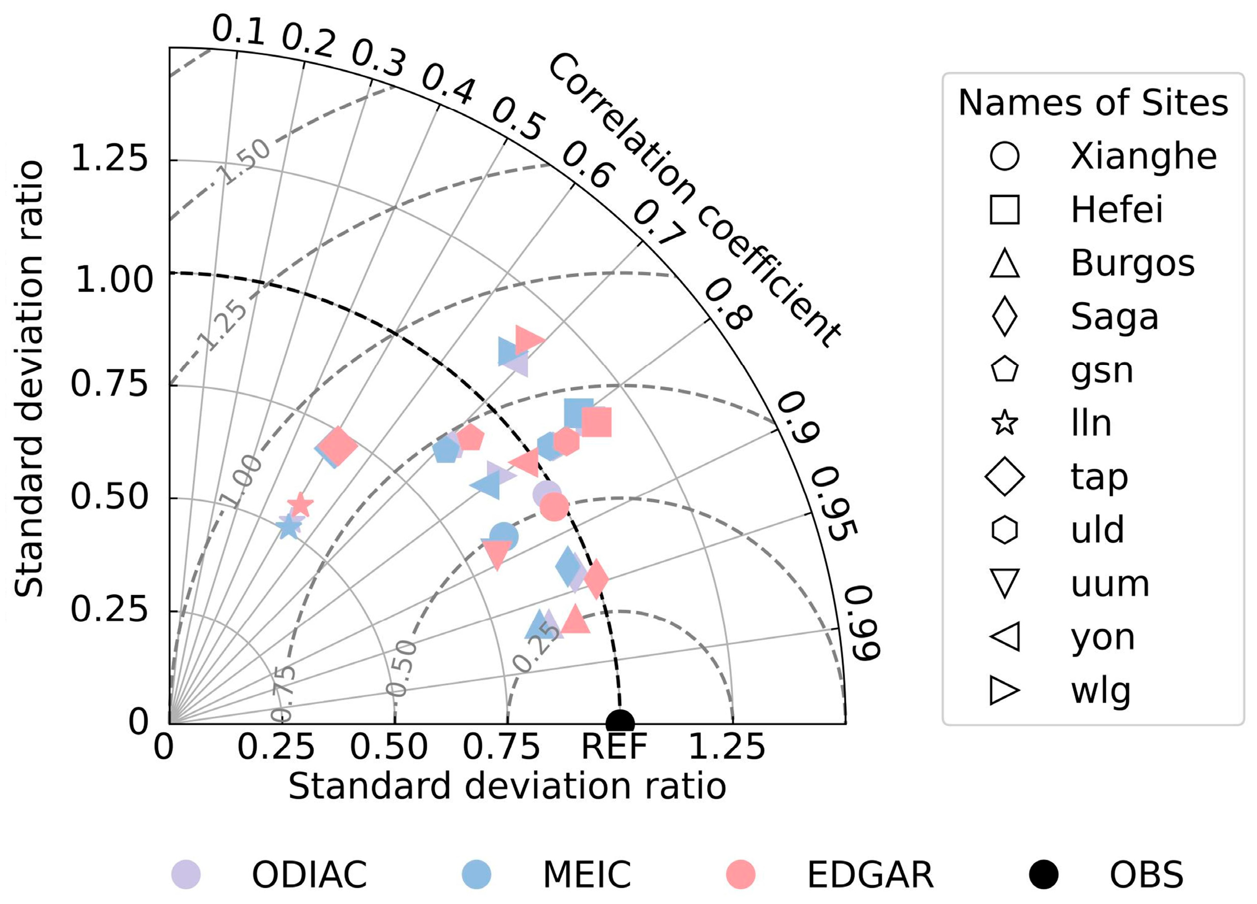
3.3. Validation with Ground-Based Observations

To assess the accuracy and seasonal variability of GEOS-Chem in simulating XCO₂ and surface CO₂ concentrations, we compared the simulated concentrations with observations from TCCON and NOAA stations across East Asia during the 2018–2020 period (Figure 5). The selected stations are geographically diverse, covering coastal, inland, and plateau environments. For each station, data from 12:00 to 14:00 local time were selected to calculate the mean concentration. The corresponding simulated CO₂ concentrations were subsequently filtered and computed. Overall, the model exhibited strong agreement with station observations, demonstrating high accuracy in capturing temporal trends and fluctuations of the observed data. The majority of stations exhibited correlation coefficient above 0.7 (

Table 2. Statistical parameters and information for each station of ground observation in 2018-2020.

Sites Name	Lat (°N)	Lon (°E)	Alt (m)	Emission Inventories	Std_r	Bias (ppm)	Correlation Coefficient
Xianghe	39.80	116.96	/	ODIAC	0.98	−0.063	0.855
				EDGAR	0.98	−0.150	0.871
				MEIC	0.95	−0.577	0.873
Hefei	31.90	117.17	/	ODIAC	1.15	−0.555	0.812
				EDGAR	1.16	0.063	0.817
				MEIC	1.14	−0.605	0.7966
Burgos	18.53	120.65	/	ODIAC	0.87	−0.989	0.967
				EDGAR	0.93	−0.704	0.968
				MEIC	0.85	−1.009	0.9656
Saga	33.24	130.29	/	ODIAC	0.96	−0.673	0.937
				EDGAR	1.00	−0.244	0.947
				MEIC	0.95	−0.704	0.930
gsn	33.28	126.15	78	ODIAC	0.880	2.209	0.713
				EDGAR	0.921	1.498	0.725
				MEIC	0.862	2.604	0.711
lln	23.46	120.86	2867	ODIAC	0.525	3.616	0.518
				EDGAR	0.565	3.300	0.514
				MEIC	0.509	3.770	0.519
tap	36.73	126.13	21	ODIAC	0.712	2.611	0.513
				EDGAR	0.721	0.942	0.518
				MEIC	0.713	2.936	0.514
uld	37.48	130.90	231	ODIAC	1.050	2.016	0.810
				EDGAR	1.081	1.379	0.815
				MEIC	1.045	2.340	0.808
uum	44.45	111.10	1012	ODIAC	0.816	2.188	0.886
				EDGAR	0.815	1.802	0.890
				MEIC	0.816	2.330	0.886
yon	24.47	123.01	50	ODIAC	1.106	0.984	0.801
				EDGAR	0.976	0.379	0.804
				MEIC	0.877	1.268	0.797
wlg	36.27	100.92	3815	ODIAC	0.920	−2.461	0.689
				EDGAR	1.169	−3.194	0.685
				MEIC	1.124	−2.423	0.678

). The correlations at lln (Lulin) and tap (Tae-ahn Peninsula) stations were approximately 0.5, possibly due to limited observation data and coastal influences, such as atmospheric transport from the ocean. The bias at TCCON stations ranged from −1.009 to −0.063 ppm, indicating strong model performance. Considering that the surface concentration model simulations were influenced by surface fluxes, particularly in large urban areas, differences of approximately 1.5 to 8 ppm from observed values are to be expected [19]. During periods of insufficient atmospheric mixing near the surface, local CO₂ concentrations may be unstable and highly variable, leading to greater fluctuations in data from ground-based observation stations. As a result, the model’s bias relative to surface CO₂ observations ranged from −3.194 to 3.770 ppm, which is within an acceptable range. At more than 80% of the stations, simulations using the EDGAR inventory demonstrated the smallest bias and highest correlation, indicating superior performance of GEOS-Chem with EDGAR flux data.

To further evaluate the performance of the three anthropogenic emission inventories, a Taylor diagram was constructed (Figure 6) to compare simulations with ground-based measurements for the 2018–2020 period. The distribution of data points on the Taylor diagram clearly visualized the relative performance of each emission inventory. At over 70% of the sites, simulations based on the three inventories demonstrated high correlations (R > 0.7, p < 0.01) with the centered root mean square error (RMSE_c) below 1.0. Simulations at the Xianghe, Saga, uld, and yon stations performed exceptionally well, with a standard deviation ratio (std_r) close to 1, correlation coefficients exceeding 0.8 (p < 0.01), and RMSE_c below 0.5, indicating strong agreement with observational data. Conversely, simulations at the lln and tap stations exhibited lower correlation coefficients and std_r. This may reflect the complex local emission characteristics and topographical influences, limiting the model’s ability to accurately reproduce conditions in these areas. Among the three inventories, the EDGAR inventory showed the best overall agreement, as indicated by the proximity of most station points to the reference point (REF) on the diagram. In summary, the comparison with ground-based observations suggested that GEOS-Chem effectively reproduced CO₂ concentrations and their temporal dynamics across most sites. However, there were notable discrepancies between the observed and simulated CO₂ concentrations at some sites. These findings highlighted the limitations of current emission inventories in terms of regional adaptability and accuracy, underscoring the need for further adjustments and optimizations tailored to different environmental characteristics.

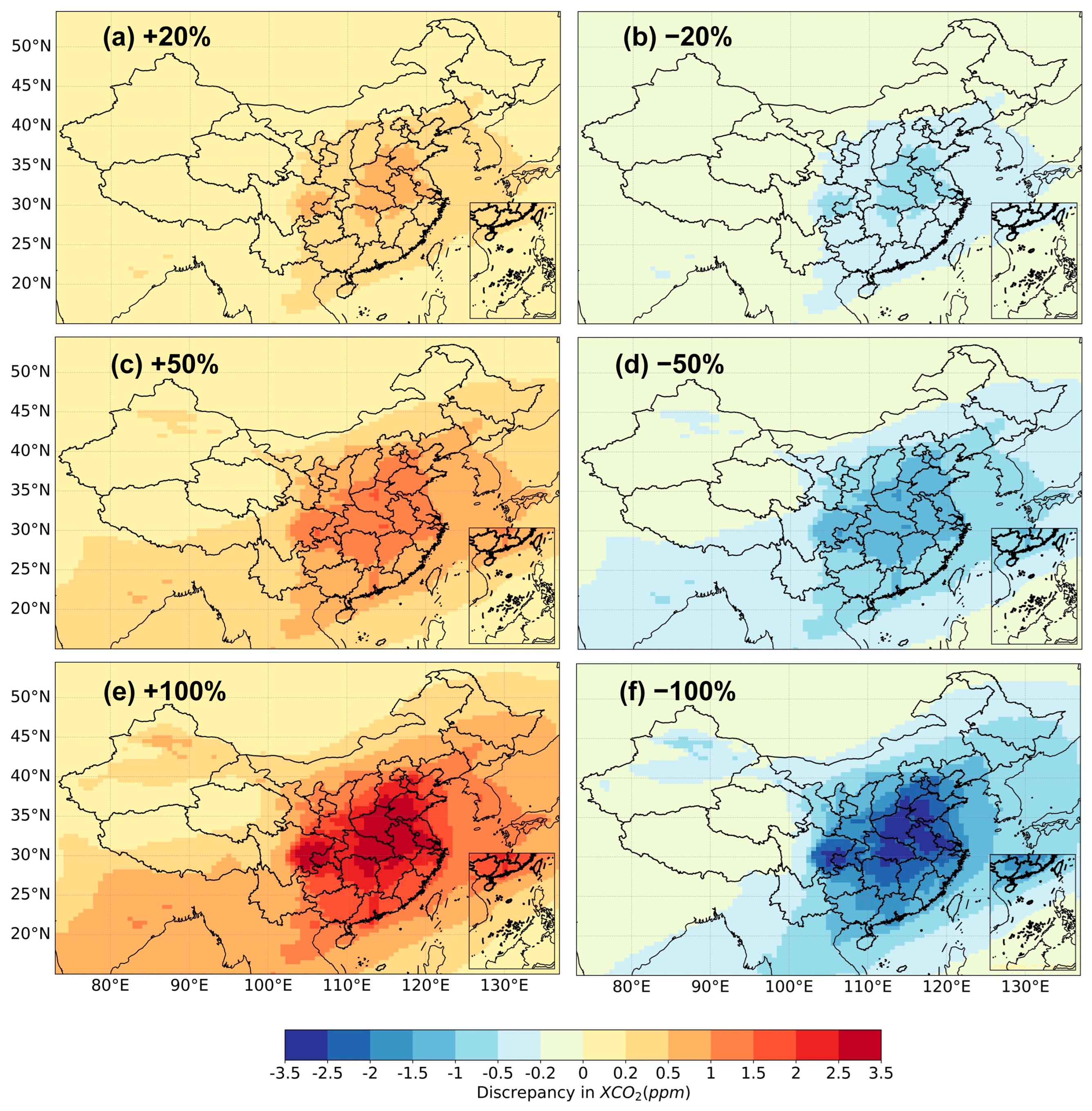
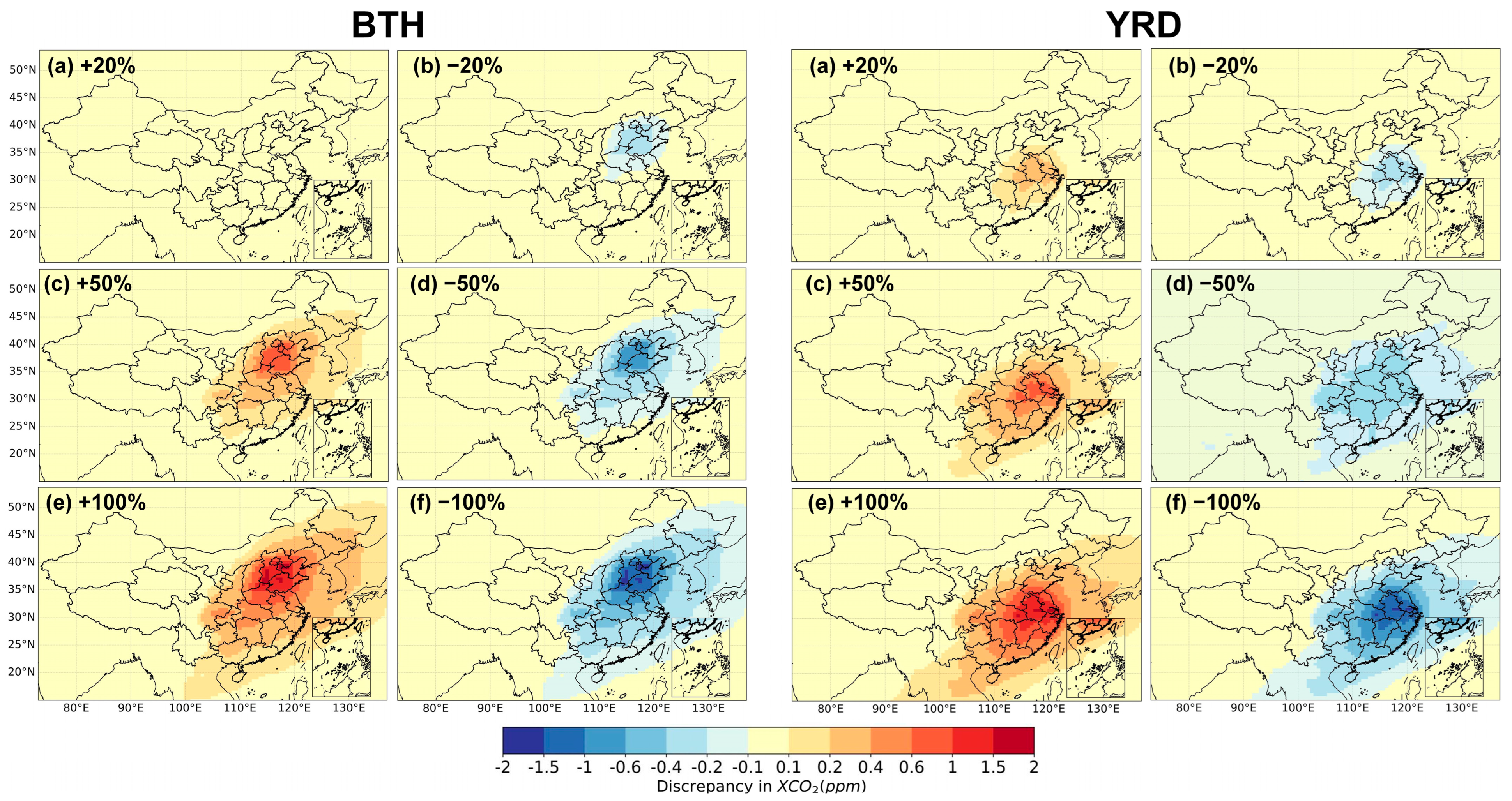
3.4. The Impact of Emission Variability on XCO₂

In this study, we conducted an experiment by turning off the fossil fuel emission option, while keeping all other parameters constant. This experiment is referred to as the “no_fossil” scenario. Figure 7 illustrates the differences between the simulation results of the three emission inventories and the no_fossil scenario, representing discrepancies attributed to anthropogenic fossil fuel emissions. The increase in XCO₂ resulting from fossil fuel combustion displays a similar spatial pattern across East Asia for all three inventories. In eastern China, particularly over the North China Plain and the Yangtze River Delta, the difference in XCO₂ reached over 10 ppm, as these regions were hotspots for anthropogenic CO₂ emissions. In contrast, concentrations were notably lower in the western regions, with XCO₂ differences ranging between 6.5 and 9 ppm. The larger increase in eastern China was attributed to its dense population and high levels of industrial activity, whereas the smaller increase in the west was associated with lower industrialization and reduced energy consumption. The XCO₂ discrepancy between the sim_EDGAR and no_fossil simulations was the largest, with a broader area showing elevated value. This could be attributed to EDGAR’s higher emission estimates compared to the other two inventories. A previous study indicated that after 2013, EDGAR’s estimates of China’s total CO₂ emissions tended to be higher compared to most other inventories [53]. Due to the inherent complexity of the atmospheric transport model, including factors like horizontal atmospheric convection, boundary layer mixing, and variations in the troposphere, the relationship between carbon dioxide emission fluxes and simulated XCO₂ concentrations is complex. Spearman’s correlation analysis [69] conducted over mainland China revealed that anthropogenic CO₂ emissions show a significant positive correlation (r > 0, p < 0.01) with simulated XCO₂ concentrations in most regions (Figure A2). However, our analysis showed that an increase in anthropogenic CO₂ flux leads to a corresponding rise in simulated XCO₂. Notably, regions with high increases in XCO₂ coincided strongly with regions of high emission intensity, indicating that our simulation reasonably reflected the spatial distribution characteristics of the emission inventories and quantifies their impact on CO₂ concentration changes.

A series of model experiments were conducted based on the EDGAR emission inventory to explore the impact of emission variability on spatial XCO₂. Specifically, the emissions in mainland China were adjusted by ±20%, ±50%, and ±100% relative to the initial EDGAR inventory. The distribution of average XCO₂ discrepancy between simulated XCO₂ for the adjusted emissions and the baseline experiment (simulated using the initial EDGAR inventory) were then analyzed. Figure 8 indicates that changes in emission levels had a significant impact on XCO₂, particularly in central and eastern China, with notable effects in regions with dense industrial activity and urbanization. As emissions increased, XCO₂ concentrations rose considerably, with the most pronounced effect observed in the +100% emission scenario (Figure 8, Panel (e)), where the XCO₂ difference reached 3.5 ppm, particularly over northern, eastern, and central China. In the +50% and +20% scenarios (Panel (c) and Panel (a)), although the increase was smaller, notable rises of 2 ppm and 1 ppm, respectively, were still observed in these key emission source regions. Conversely, under emission reduction scenarios, XCO₂ concentrations decreased to varying degrees. Figure 8, Panel (c) shows that XCO₂ concentrations in the eastern seaboard urban agglomeration dropped to −2 ppm in the −50% scenario. In the −50% scenario, the XCO₂ concentration was observed to decrease by −2 ppm in the eastern coastal urban clusters. When the emissions in the mainland China region were reduced by 100%, the discrepancy in XCO₂ between the adjusted simulation and the baseline experiment in eastern China could reach 2 to 3.5 ppm. This underscores the dominant role of these regions in emissions, where emission reductions have a significant impact on XCO₂ concentrations. It is worth noting that even when only the emissions for mainland China were changed, there were still differences observed in regions such as the Bohai Sea, the Yellow Sea, and Southeast Asia, where the emission flux remained unchanged compared to the baseline experiment. This suggests that changes in CO₂ emissions in mainland China may have an impact on the CO₂ concentrations in neighboring countries and surrounding seas due to atmospheric transport. Overall, the results highlighted a clear spatial heterogeneity in the response of XCO₂ concentrations to changes in emission levels, with more pronounced effects in high-emission regions. The nonlinear response across different areas highlighted the critical role of carbon concentrations in high-emission regions in regulating atmospheric XCO₂ levels. Targeted emission control in central China, in particular, could not only reduce XCO₂ concentrations within the region but also curb the rising trend of CO₂ concentrations over a broader spatial scale.

We separately conducted simulation experiments by modifying the emissions in the BTH and YRD regions to analyze the impact of emission changes in these urban clusters on the XCO₂ concentrations in the region and its surrounding areas. Compared to nationwide emission adjustments, changes in emissions within the BTH region exhibited a more localized and concentrated influence on XCO₂ (Figure 9). This impact was primarily confined to the North China area, although its intensity and magnitude remained significant. In the +100% emissions scenario (BTH, Panel (e)), the increase in XCO₂ was most pronounced, with the maximum rise ranging from approximately 1.5 to 2 ppm, concentrated in the industrial and densely populated areas of Beijing, Tianjin, and central Hebei. As emissions were reduced, the extent and intensity of the impact diminished progressively. As shown in BTH, Panel (c), the area of concentration growth became smaller in the +50% scenario, with the intensity diminishing to 0.4–1.5 ppm. The effect remained concentrated in the BTH region, with minor expansion into neighboring provinces. When emissions were increased by 20% (BTH, Panel (a)), the resulting change in XCO₂ was minimal, resulting in changes of less than 0.1 ppm. On the other hand, in emissions reduction scenarios, the decline in XCO₂ was similarly concentrated in the BTH region. Under the −20% emissions scenario, the XCO₂ decrease ranged from −0.2 to −0.4 ppm, with a limited area of influence, mainly covering a small portion of the BTH surroundings. In the −50% and −100% emissions scenarios ((Panel (d) and Panel (f), respectively)), the decrease became more significant, with the largest difference ranging from −1 to −2 ppm. The affected area expanded into the surrounding North China Plain, particularly northern Hebei and Shandong provinces, demonstrating a clear regional impact. This suggested that changes in emissions within the BTH region had a significant localized effect on the spatial distribution of XCO₂. Although the scope of influence was smaller compared to national emission adjustments, the impact on atmospheric carbon concentration in the area was substantial, especially under high-emission scenarios.

In the YRD region, increases in emissions predominantly affected XCO₂ concentrations in Jiangsu, Shanghai, and Zhejiang, with a maximum increase of 1.5 to 2 ppm in the +100% emissions scenario (YRD, Panel (e)). When emissions were adjusted by 20%, the impact on the YRD and its surrounding areas ranged from −0.4 to 0.4 ppm, with the affected area limited to the YRD and adjacent inland cities (YRD, Panel (a) and Panel (b)). As the magnitude of emission changes increased, the impact gradually extended to parts of Anhui, Jiangxi, and Fujian, with a clear influence on XCO₂ levels in the eastern coastal regions of China. This indicated that while emissions were altered only in the YRD, atmospheric circulation and exchange influenced CO₂ concentrations in marine areas. Overall, compared to nationwide emission changes, adjustments to emissions in the BTH and YRD regions primarily influenced the local areas and their surroundings, with a more concentrated intensity and relatively smaller spatial extent. However, regional emission changes could significantly alter the XCO₂ distribution in these areas. Therefore, carbon reduction policies in the BTH region are essential for regulating atmospheric CO₂ concentrations.

4. Conclusions

This study evaluated variations in anthropogenic CO₂ emissions across mainland China from 2018 to 2020 and their impact on atmospheric CO₂ concentrations. The study conducted a comparative analysis of three commonly utilized emission inventories—ODIAC, MEIC, and EDGAR. Chemical transport models were employed to simulate CO₂ concentrations, integrated with both satellite and ground-based observation data. Additionally, numerical experiments to analyze the impacts of emission level variations on the spatiotemporal distribution of CO₂ were conducted. The results underscored the vital role of accurate emission inventories, as discrepancies between these datasets significantly affect simulations of atmospheric CO₂ concentrations. This research aims to clarify the substantial influence of anthropogenic CO₂ emissions on atmospheric CO₂ concentrations and their response to emission variations, highlighting the need for improved emission inventories.

The spatial distribution of emissions across the three inventories exhibited consistent patterns. Higher emissions were observed in economically developed coastal regions, such as the North China Plain and the Yangtze River Delta, while lower emissions were found in the western regions. However, differences in spatial resolution and regional emissions were evident between the inventories. The study found that these discrepancies led to notable differences in simulated CO₂ concentrations over China and neighboring regions, particularly in areas with high emission values. Additionally, model performance was evaluated against ground-based station and satellite observations, with EDGAR showing the best consistency. The majority of the deviations between EDGAR and satellite observations ranged from −1 to 2 ppm, with an average bias of 0.31 ppm.

Moreover, a series of numerical experiments demonstrated that variations in emission levels significantly influence CO₂ concentrations, especially in industrialized and densely populated regions. In the “no_fossil” experiment, where anthropogenic emissions were disabled, the difference in XCO₂ between the North China Plain and the Yangtze River Delta regions and the base experiment exceeded 10 ppm, as these areas are hotspots for anthropogenic CO₂ emissions. In the scenario where emissions increased by 100%, the XCO₂ differences were most pronounced, reaching up to 3.5 ppm, with the pronounced discrepancies concentrated in northern and central China. In high-emission regions like the Yangtze River Delta and BTH areas, this increase in emissions induced significant changes in atmospheric CO₂ levels. When emissions were adjusted by ±100% in the BTH and Yangtze River Delta regions, the XCO₂ variations reached as high as 2 ppm, and these changes also influenced CO₂ concentrations in adjacent regions with unchanged emissions. This finding was particularly important for China, where localized emission reductions in key regions can have profound impacts on national and regional atmospheric CO₂ levels.

This study may contribute to understanding the impact of anthropogenic CO₂ emissions on atmospheric CO₂ concentrations and provide a reference for selecting of anthropogenic emission inventories in forward CO₂ simulations. However, there were some uncertainties in this research. The meteorological data used in the model, along with biomass burning emission inventories, land carbon flux data, and other inputs, may have influenced the simulation results. Furthermore, different atmospheric chemistry models employ distinct chemical transport mechanisms. Therefore, future research exploring simulations using a variety of atmospheric chemistry models would be valuable. Additionally, the estimates of fossil fuel emissions are highly uncertain, and the accuracy of emission inventories significantly influences the simulated atmospheric CO₂ concentrations. If fossil fuel emissions are not adequately corrected during the inversion process, errors in these emissions will be redistributed to the estimates of other natural biosphere fluxes [70]. Therefore, future research should aim to obtain more reliable fossil fuel emission inventories and enhance the quantification of inventory uncertainties, incorporating the associated uncertainties of fossil fuel emissions into the inversion framework.

References

1. Lan, X.; Tans, P.; Thoning, K.W. Trends in Globally-Averaged CO2 Determined from NOAA Global Monitoring Laboratory Measurements. Available online: https://gml.noaa.gov/ccgg/trends/gl_data.html (accessed on 1 December 2024).
2. Manabe, S.; Wetherald, R.T. Thermal Equilibrium of the Atmosphere with a Given Distribution of Relative Humidity. J. Atmos. Sci. 1967, 24, 241–259. [Google Scholar] [CrossRef]
3. Gunter, W.D.; Wong, S.; Cheel, D.B.; Sjostrom, G. Large CO2 Sinks: Their role in the mitigation of greenhouse gases from an international, national (Canadian) and provincial (Alberta) perspective. Appl. Energy 1998, 61, 209–227. [Google Scholar] [CrossRef]
4. IPCC. Climate Change 2021: The Physical Science Basis. Contribution of Working Group I to the Sixth Assessment Report of the Intergovernmental Panel on Climate Change; Cambridge University Press: Cambridge, UK, 2021. [Google Scholar]
5. Friedlingstein, P.; O’Sullivan, M.; Jones, M.W.; Andrew, R.M.; Bakker, D.C.E.; Hauck, J.; Landschützer, P.; Le Quéré, C.; Luijkx, I.T.; Peters, G.P.; et al. Global Carbon Budget 2023. Earth Syst. Sci. Data 2023, 15, 5301–5369. [Google Scholar] [CrossRef]
6. Schimel, D. Carbon cycle conundrums. Proc. Natl. Acad. Sci. USA 2007, 104, 18353–18354. [Google Scholar] [CrossRef]
7. Kou, X.; Zhang, M.; Peng, Z.; Wang, Y. Assessment of the biospheric contribution to surface atmospheric CO2 concentrations over East Asia with a regional chemical transport model. Adv. Atmos. Sci. 2015, 32, 287–300. [Google Scholar] [CrossRef]
8. Fu, Y.; Liao, H.; Tian, X.; Gao, H.; Jia, B.; Han, R. Impact of Prior Terrestrial Carbon Fluxes on Simulations of Atmospheric CO2 Concentrations. J. Geophys. Res. Atmos. 2021, 126, e2021JD034794. [Google Scholar] [CrossRef]
9. Andres, R.J.; Boden, T.A.; Higdon, D. A new evaluation of the uncertainty associated with CDIAC estimates of fossil fuel carbon dioxide emission. Tellus B Chem. Phys. Meteorol. 2014, 66, 23616. [Google Scholar] [CrossRef]
10. Crippa, M.; Guizzardi, D.; Banja, M.; Solazzo, E.; Muntean, M.; Schaaf, E.; Pagani, F.; Monforti, F.; Olivier, J.; Quadrelli, R.; et al. CO2 Emissions of All World Countries; JRC/IEA/PBL 2022 Report; Publications Office of the European Union: Luxembourg, 2022. [Google Scholar]
11. Solazzo, E.; Crippa, M.; Guizzardi, D.; Muntean, M.; Choulga, M.; Janssens-Maenhout, G. Uncertainties in the Emissions Database for Global Atmospheric Research (EDGAR) emission inventory of greenhouse gases. Atmos. Chem. Phys. 2021, 21, 5655–5683. [Google Scholar] [CrossRef]
12. Marland, G. China’s uncertain CO2 emissions. Nat. Clim. Change 2012, 2, 645–646. [Google Scholar] [CrossRef]
13. Gregg, J.S.; Andres, R.J.; Marland, G. China: Emissions pattern of the world leader in CO2 emissions from fossil fuel consumption and cement production. Geophys. Res. Lett. 2008, 35, L08806. [Google Scholar] [CrossRef]
14. Andres, R.J.; Boden, T.A.; Bréon, F.M.; Ciais, P.; Davis, S.; Erickson, D.; Gregg, J.S.; Jacobson, A.; Marland, G.; Miller, J.; et al. A synthesis of carbon dioxide emissions from fossil-fuel combustion. Biogeosciences 2012, 9, 1845–1871. [Google Scholar] [CrossRef]
15. Liu, Z.; Deng, Z.; He, G.; Wang, H.; Zhang, X.; Lin, J.; Qi, Y.; Liang, X. Challenges and opportunities for carbon neutrality in China. Nat. Rev. Earth Environ. 2021, 3, 141–155. [Google Scholar] [CrossRef]
16. Shan, Y.; Guan, D.; Zheng, H.; Ou, J.; Li, Y.; Meng, J.; Mi, Z.; Liu, Z.; Zhang, Q. China CO2 emission accounts 1997–2015. Sci. Data 2018, 5, 170201. [Google Scholar] [CrossRef]
17. Guan, D.; Liu, Z.; Geng, Y.; Lindner, S.; Klaus, H. The gigatonne gap in China’s carbon dioxide inventories. Nat. Clim. Change 2012, 2, 672–675. [Google Scholar] [CrossRef]
18. Liu, Z.; Guan, D.; Wei, W.; Davis, S.J.; Ciais, P.; Bai, J.; Peng, S.; Zhang, Q.; Hubacek, K.; Marland, G.; et al. Reduced carbon emission estimates from fossil fuel combustion and cement production in China. Nature 2015, 524, 335–338. [Google Scholar] [CrossRef]
19. Nassar, R.; Napier-Linton, L.; Gurney, K.R.; Andres, R.J.; Oda, T.; Vogel, F.R.; Deng, F. Improving the temporal and spatial distribution of CO2 emissions from global fossil fuel emission data sets. J. Geophys. Res. Atmos. 2013, 118, 917–933. [Google Scholar] [CrossRef]
20. Gurney, K.R.; Law, R.M.; Denning, A.S.; Rayner, P.J.; Baker, D.; Bousquet, P.; Bruhwiler, L.; Chen, Y.-H.; Ciais, P.; Fan, S.; et al. TransCom 3 CO2 inversion intercomparison: 1. Annual mean control results and sensitivity to transport and prior flux information. Tellus B 2003, 55, 555–579. [Google Scholar] [CrossRef]
21. O’Dell, C.W.; Eldering, A.; Wennberg, P.O.; Crisp, D.; Gunson, M.R.; Fisher, B.; Frankenberg, C.; Kiel, M.; Lindqvist, H.; Mandrake, L.; et al. Improved retrievals of carbon dioxide from Orbiting Carbon Observatory-2 with the version 8 ACOS algorithm. Atmos. Meas. Tech. 2018, 11, 6539–6576. [Google Scholar] [CrossRef]
22. Yokota, T.; Yoshida, Y.; Eguchi, N.; Ota, Y.; Tanaka, T.; Watanabe, H.; Maksyutov, S. Global Concentrations of CO2 and CH4 Retrieved from GOSAT: First Preliminary Results. SOLA 2009, 5, 160–163. [Google Scholar] [CrossRef]
23. Liu, Y.; Wang, J.; Yao, L.; Chen, X.; Cai, Z.; Yang, D.; Yin, Z.; Gu, S.; Tian, L.; Lu, N.; et al. The TanSat mission: Preliminary global observations. Sci. Bull. 2018, 63, 1200–1207. [Google Scholar] [CrossRef] [PubMed]
24. Wunch, D.; Toon, G.C.; Blavier, J.-F.L.; Washenfelder, R.A.; Notholt, J.; Connor, B.J.; Griffith, D.W.T.; Sherlock, V.; Wennberg, P.O. The Total Carbon Column Observing Network. Philos. Trans. R. Soc. A Math. Phys. Eng. Sci. 2011, 369, 2087–2112. [Google Scholar] [CrossRef]
25. Frey, M.; Sha, M.K.; Hase, F.; Kiel, M.; Blumenstock, T.; Harig, R.; Surawicz, G.; Deutscher, N.M.; Shiomi, K.; Franklin, J.E.; et al. Building the COllaborative Carbon Column Observing Network (COCCON): Long-term stability and ensemble performance of the EM27/SUN Fourier transform spectrometer. Atmos. Meas. Tech. 2019, 12, 1513–1530. [Google Scholar] [CrossRef]
26. Jing, Y.; Shi, J.; Wang, T. Evaluation and comparison of atmospheric CO2 concentrations from models and satellite retrievals. In Proceedings of the 2015 IEEE International Geoscience and Remote Sensing Symposium (IGARSS), Milan, Italy, 26–31 July 2015; pp. 2202–2205. [Google Scholar]
27. Zhang, H.; Chen, B.; Xu, G.; Yan, J.; Che, M.; Chen, J.; Fang, S.; Lin, X.; Sun, S. Comparing simulated atmospheric carbon dioxide concentration with GOSAT retrievals. Sci. Bull. 2015, 60, 380–386. [Google Scholar] [CrossRef]
28. Lei, L.; Guan, X.; Zeng, Z.; Zhang, B.; Ru, F.; Bu, R. A comparison of atmospheric CO2 concentration GOSAT-based observations and model simulations. Sci. China Earth Sci. 2014, 57, 1393–1402. [Google Scholar] [CrossRef]
29. Li, R.; Zhang, M.; Chen, L.; Kou, X.; Skorokhod, A. CMAQ simulation of atmospheric CO2 concentration in East Asia: Comparison with GOSAT observations and ground measurements. Atmos. Environ. 2017, 160, 176–185. [Google Scholar] [CrossRef]
30. Ma, X.-Y.; Huang, W.-J.; Hu, N.; Xiao, W.; Hu, C.; Zhang, M.; Cao, C.; Zhao, J.-Y. Simulation of Anthropogenic CO2 Emissions in the Yangtze River Delta Based on Different Emission Inventories. Environ. Sci. 2023, 44, 2009–2021. [Google Scholar] [CrossRef]
31. Zhang, S.; Tian, X. The impacts of modeling global CO2 concentrations with GEOS-Chem using different ocean carbon fluxes. Atmos. Ocean. Sci. Lett. 2019, 12, 343–348. [Google Scholar] [CrossRef]
32. Su, M.; Shi, Y.; Yang, Y.; Guo, W. Impacts of different biomass burning emission inventories: Simulations of atmospheric CO2 concentrations based on GEOS-Chem. Sci. Total Environ. 2023, 876, 162825. [Google Scholar] [CrossRef] [PubMed]
33. Ciais, P.; Rayner, P.; Chevallier, F.; Bousquet, P.; Logan, M.; Peylin, P.; Ramonet, M. Atmospheric inversions for estimating CO2 fluxes: Methods and perspectives. Clim. Change 2010, 103, 69–92. [Google Scholar] [CrossRef]
34. Yang, D.; Liu, Y.; Feng, L.; Wang, J.; Yao, L.; Cai, Z.; Zhu, S.; Lu, N.; Lyu, D. The First Global Carbon Dioxide Flux Map Derived from TanSat Measurements. Adv. Atmos. Sci. 2021, 38, 1433–1443. [Google Scholar] [CrossRef]
35. Kong, Y.; Zheng, B.; Zhang, Q.; He, K. Global and regional carbon budget for 2015–2020 inferred from OCO-2 based on an ensemble Kalman filter coupled with GEOS-Chem. Atmos. Chem. Phys. 2022, 22, 10769–10788. [Google Scholar] [CrossRef]
36. Suntharalingam, P.; Jacob, D.J.; Palmer, P.I.; Logan, J.A.; Yantosca, R.M.; Xiao, Y.; Evans, M.J.; Streets, D.G.; Vay, S.L.; Sachse, G.W. Improved quantification of Chinese carbon fluxes using CO2/CO correlations in Asian outflow. J. Geophys. Res. Atmos. 2004, 109, D18S18. [Google Scholar] [CrossRef]
37. Nassar, R.; Jones, D.B.A.; Suntharalingam, P.; Chen, J.M.; Andres, R.J.; Wecht, K.J.; Yantosca, R.M.; Kulawik, S.S.; Bowman, K.W.; Worden, J.R.; et al. Modeling global atmospheric CO2 with improved emission inventories and CO2 production from the oxidation of other carbon species. Geosci. Model Dev. 2010, 3, 689–716. [Google Scholar] [CrossRef]
38. Oda, T.; Maksyutov, S. A very high-resolution (1 km × 1 km) global fossil fuel CO2 emission inventory derived using a point source database and satellite observations of nighttime lights. Atmos. Chem. Phys. 2011, 11, 543–556. [Google Scholar] [CrossRef]
39. Zheng, B.; Tong, D.; Li, M.; Liu, F.; Hong, C.; Geng, G.; Li, H.; Li, X.; Peng, L.; Qi, J.; et al. Trends in China’s anthropogenic emissions since 2010 as the consequence of clean air actions. Atmos. Chem. Phys. 2018, 18, 14095–14111. [Google Scholar] [CrossRef]
40. Li, M.; Liu, H.; Geng, G.; Hong, C.; Liu, F.; Song, Y.; Tong, D.; Zheng, B.; Cui, H.; Man, H.; et al. Anthropogenic emission inventories in China: A review. Natl. Sci. Rev. 2017, 4, 834–866. [Google Scholar] [CrossRef]
41. van der Werf, G.R.; Randerson, J.T.; Giglio, L.; van Leeuwen, T.T.; Chen, Y.; Rogers, B.M.; Mu, M.; van Marle, M.J.E.; Morton, D.C.; Collatz, G.J.; et al. Global fire emissions estimates during 1997–2016. Earth Syst. Sci. Data 2017, 9, 697–720. [Google Scholar] [CrossRef]
42. Takahashi, T.; Sutherland, S.C.; Wanninkhof, R.; Sweeney, C.; Feely, R.A.; Chipman, D.W.; Hales, B.; Friederich, G.; Chavez, F.; Sabine, C.; et al. Climatological mean and decadal change in surface ocean pCO2, and net sea–air CO2 flux over the global oceans. Deep. Sea Res. Part II Top. Stud. Oceanogr. 2009, 56, 554–577. [Google Scholar] [CrossRef]
43. Messerschmidt, J.; Parazoo, N.; Wunch, D.; Deutscher, N.M.; Roehl, C.; Warneke, T.; Wennberg, P.O. Evaluation of seasonal atmosphere–biosphere exchange estimations with TCCON measurements. Atmos. Chem. Phys. 2013, 13, 5103–5115. [Google Scholar] [CrossRef]
44. Baker, D.F.; Law, R.M.; Gurney, K.R.; Rayner, P.; Peylin, P.; Denning, A.S.; Bousquet, P.; Bruhwiler, L.; Chen, Y.H.; Ciais, P.; et al. TransCom 3 inversion intercomparison: Impact of transport model errors on the interannual variability of regional CO2 fluxes, 1988–2003. Glob. Biogeochem. Cycles 2006, 20, GB1002. [Google Scholar] [CrossRef]
45. Hoesly, R.M.; Smith, S.J.; Feng, L.; Klimont, Z.; Janssens-Maenhout, G.; Pitkanen, T.; Seibert, J.J.; Vu, L.; Andres, R.J.; Bolt, R.M.; et al. Historical (1750–2014) anthropogenic emissions of reactive gases and aerosols from the Community Emissions Data System (CEDS). Geosci. Model Dev. 2018, 11, 369–408. [Google Scholar] [CrossRef]
46. Simone, N.W.; Stettler, M.E.J.; Barrett, S.R.H. Rapid estimation of global civil aviation emissions with uncertainty quantification. Transp. Res. Part D Transp. Environ. 2013, 25, 33–41. [Google Scholar] [CrossRef]
47. Olsen, S.C.; Brasseur, G.P.; Wuebbles, D.J.; Barrett, S.R.H.; Dang, H.; Eastham, S.D.; Jacobson, M.Z.; Khodayari, A.; Selkirk, H.; Sokolov, A.; et al. Comparison of model estimates of the effects of aviation emissions on atmospheric ozone and methane. Geophys. Res. Lett. 2013, 40, 6004–6009. [Google Scholar] [CrossRef]
48. Reddington, C.L.; Conibear, L.; Robinson, S.; Knote, C.; Arnold, S.R.; Spracklen, D.V. Air Pollution from Forest and Vegetation Fires in Southeast Asia Disproportionately Impacts the Poor. GeoHealth 2021, 5, e2021GH000418. [Google Scholar] [CrossRef] [PubMed]
49. Oda, T.; Maksyutov, S. ODIAC Fossil Fuel CO2 Emissions Dataset (Version Name: ODIAC2022); Center for Global Environmental Research, National Institute for Environmental Studies: Tsukuba, Japan, 2015. [Google Scholar] [CrossRef]
50. Oda, T.; Maksyutov, S.; Andres, R.J. The Open-source Data Inventory for Anthropogenic CO2, version 2016 (ODIAC2016): A global monthly fossil fuel CO2 gridded emissions data product for tracer transport simulations and surface flux inversions. Earth Syst. Sci. Data 2018, 10, 87–107. [Google Scholar] [CrossRef]
51. Wheeler, D.; Ummel, K. Calculating CARMA: Global Estimation of CO2 Emissions from the Power Sector; Working Papers; Center for Global Development: Washington, DC, USA, 2008. [Google Scholar] [CrossRef]
52. Raupach, M.R.; Rayner, P.J.; Paget, M. Regional variations in spatial structure of nightlights, population density and fossil-fuel CO2 emissions. Energy Policy 2010, 38, 4756–4764. [Google Scholar] [CrossRef]
53. Han, P.; Zeng, N.; Oda, T.; Lin, X.; Crippa, M.; Guan, D.; Janssens-Maenhout, G.; Ma, X.; Liu, Z.; Shan, Y.; et al. Evaluating China’s fossil-fuel CO2 emissions from a comprehensive dataset of nine inventories. Atmos. Chem. Phys. 2020, 20, 11371–11385. [Google Scholar] [CrossRef]
54. Wunch, D.; Wennberg, P.O.; Osterman, G.; Fisher, B.; Naylor, B.; Roehl, C.M.; O’Dell, C.; Mandrake, L.; Viatte, C.; Kiel, M.; et al. Comparisons of the Orbiting Carbon Observatory-2 (OCO-2) XCO2 measurements with TCCON. Atmos. Meas. Tech. 2017, 10, 2209–2238. [Google Scholar] [CrossRef]
55. Labzovskii, L.D.; Jeong, S.-J.; Parazoo, N.C. Working towards confident spaceborne monitoring of carbon emissions from cities using Orbiting Carbon Observatory-2. Remote Sens. Environ. 2019, 233, 111359. [Google Scholar] [CrossRef]
56. Kiel, M.; O’Dell, C.W.; Fisher, B.; Eldering, A.; Nassar, R.; MacDonald, C.G.; Wennberg, P.O. How bias correction goes wrong: Measurement of XCO2 affected by erroneous surface pressure estimates. Atmos. Meas. Tech. 2019, 12, 2241–2259. [Google Scholar] [CrossRef]
57. Connor, B.J.; Boesch, H.; Toon, G.; Sen, B.; Miller, C.; Crisp, D. Orbiting Carbon Observatory: Inverse method and prospective error analysis. J. Geophys. Res. Atmos. 2008, 113, D05305. [Google Scholar] [CrossRef]
58. Buschmann, M.; Deutscher, N.M.; Sherlock, V.; Palm, M.; Warneke, T.; Notholt, J. Retrieval of xCO2 from ground-based mid-infrared (NDACC) solar absorption spectra and comparison to TCCON. Atmos. Meas. Tech. 2016, 9, 577–585. [Google Scholar] [CrossRef]
59. Laughner, J.L.; Toon, G.C.; Mendonca, J.; Petri, C.; Roche, S.; Wunch, D.; Blavier, J.F.; Griffith, D.W.T.; Heikkinen, P.; Keeling, R.F.; et al. The Total Carbon Column Observing Network’s GGG2020 data version. Earth Syst. Sci. Data 2024, 16, 2197–2260. [Google Scholar] [CrossRef]
60. Morino, I.; Velasco, V.A.; Hori, A.; Uchino, O.; Griffith, D.W.T. TCCON Data from Burgos, Ilocos Norte (PH), Release GGG2020.R0; CaltechDATA: Pasadena, CA, USA, 2022. [Google Scholar] [CrossRef]
61. Liu, C.; Wang, W.; Sun, Y.; Shan, C. TCCON Data from Hefei (PRC), Release GGG2020.R1; CaltechDATA: Pasadena, CA, USA, 2023. [Google Scholar] [CrossRef]
62. Shiomi, K.; Kawakami, S.; Ohyama, H.; Arai, K.; Okumura, H.; Ikegami, H.; Usami, M. TCCON Data from Saga (JP), Release GGG2020.R0; CaltechDATA: Pasadena, CA, USA, 2022. [Google Scholar] [CrossRef]
63. Zhou, M.; Wang, P.; Kumps, N.; Hermans, C.; Nan, W. TCCON Data from Xianghe, China, Release GGG2020.R0; CaltechDATA: Pasadena, CA, USA, 2022. [Google Scholar] [CrossRef]
64. Lan, X.; Mund, J.W.; Crotwell, A.M.; Thoning, K.W.; Moglia, E.; Madronich, M.; Baugh, K.; Petron, G.; Crotwell, M.J.; Neff, D.; et al. Atmospheric Carbon Dioxide Dry Air Mole Fractions from the NOAA GML Carbon Cycle Cooperative Global Air Sampling Network, 1968–2023; National Oceanic and Atmospheric Administration, Global Monitoring Laboratory (NOAA/GML): Boulder, CO, USA, 2024; Version: 2024-07-30. [CrossRef]
65. Fu, Y.; Liao, H.; Tian, X.-J.; Gao, H.; Cai, Z.-N.; Han, R. Sensitivity of the simulated CO2 concentration to inter-annual variations of its sources and sinks over East Asia. Adv. Clim. Change Res. 2019, 10, 250–263. [Google Scholar] [CrossRef]
66. Taylor, K.E. Summarizing multiple aspects of model performance in a single diagram. J. Geophys. Res. Atmos. 2001, 106, 7183–7192. [Google Scholar] [CrossRef]
67. Lv, Z.; Shi, Y.; Zang, S.; Sun, L. Spatial and Temporal Variations of Atmospheric CO2 Concentration in China and Its Influencing Factors. Atmosphere 2020, 11, 231. [Google Scholar] [CrossRef]
68. Mustafa, F.; Bu, L.; Wang, Q.; Ali, M.A.; Bilal, M.; Shahzaman, M.; Qiu, Z. Multi-Year Comparison of CO2 Concentration from NOAA Carbon Tracker Reanalysis Model with Data from GOSAT and OCO-2 over Asia. Remote Sens. 2020, 12, 2498. [Google Scholar] [CrossRef]
69. Spearman, C. The proof and measurement of association between two things. Am. J. Psychol. 1904, 15, 72–101. [Google Scholar] [CrossRef]
70. Oda, T.; Feng, L.; Palmer, P.; Baker, D.; Ott, L. Assumptions about prior fossil fuel inventories impact our ability to estimate posterior net CO2 fluxes that are needed for verifying national inventories. Environ. Res. Lett. 2023, 18, 124030. [Google Scholar] [CrossRef]
71. Friedlingstein, P.; Jones, M.W.; O’Sullivan, M.; Andrew, R.M.; Hauck, J.; Peters, G.P.; Peters, W.; Pongratz, J.; Sitch, S.; Le Quéré, C.; et al. Global Carbon Budget 2019. Earth Syst. Sci. Data 2019, 11, 1783–1838. [Google Scholar] [CrossRef]
72. Friedlingstein, P.; O’Sullivan, M.; Jones, M.W.; Andrew, R.M.; Hauck, J.; Olsen, A.; Peters, G.P.; Peters, W.; Pongratz, J.; Sitch, S.; et al. Global Carbon Budget 2020. Earth Syst. Sci. Data 2020, 12, 3269–3340. [Google Scholar] [CrossRef]
73. Friedlingstein, P.; Jones, M.W.; O’Sullivan, M.; Andrew, R.M.; Bakker, D.C.E.; Hauck, J.; Le Quéré, C.; Peters, G.P.; Peters, W.; Pongratz, J.; et al. Global Carbon Budget 2021. Earth Syst. Sci. Data 2022, 14, 1917–2005. [Google Scholar] [CrossRef]
74. Olivier, J.; Peters, J. Trend in Global CO2 and GHG Emissions—2019 Report; PBL Report; PBL Netherlands Environmental Assessment Agency: The Hague, The Netherlands, 2019. [Google Scholar]
75. Olivier, J.; Peters, J. Trend in Global CO2 and GHG Emissions—2020 Report; PBL Report; PBL Netherlands Environmental Assessment Agency: The Hague, The Netherlands, 2020. [Google Scholar]
76. Olivier, J.; Peters, J. Trend in Global CO2 and GHG Emissions—2021 Report; PBL Report; PBL Netherlands Environmental Assessment Agency: The Hague, The Netherlands, 2021. [Google Scholar]
77. O’Rourke, P.R.; Smith, S.J.; Mott, A.; Ahsan, H.; McDuffie, E.E.; Crippa, M.; Klimont, Z.; McDonald, B.; Wang, S.; Nicholson, M.B.; et al. CEDS v_2021_04_21; Release Emission Data (v_2021_02_05); Zenodo: Geneva, Switzerland, 2021. [Google Scholar] [CrossRef]
Figure 1. Spatial distribution of emissions (gC/m2/d) in mainland China from three inventories in 2018–2020: (a) ODIAC, (b) MEIC and (c) EDGAR, with zoomed-in views of the BTH and YRD regions in the right panel.
Remotesensing 17 00814 g001
Figure 2. Time series of monthly anthropogenic CO2 emissions over mainland China from 2018 to 2020 based on three emission inventories: ODIAC, MEIC, and EDGAR.
Remotesensing 17 00814 g002
Figure 3. Distribution of mean XCO2 for three emission inventories (ODIAC, MEIC, and EDGAR) simulations (first column) and discrepancy between each of the three simulations and the mean (second to fourth columns) in 2018–2020 (ANN: annual; MAM: March–April-May; JJA: June–July–August; SON: September–October–November; DJF: December–February).
Remotesensing 17 00814 g003
Figure 4. Bias (XCO2_OCO minus XCO2_Sim) distributions of satellite XCO2 observations and model simulations for ANN, MAM, JJA, SON and DJF in 2020, with the first, second, and third columns showing the differences between observations and simulations based on the ODIAC, MEIC, and EDGAR inventories ((a) Obs minus Sim_ODIAC, (b) Obs minus Sim_MEIC, and (c) Obs minus Sim_EDGAR).
Remotesensing 17 00814 g004
Figure 5. Geophysical locations of the selected sites.
Remotesensing 17 00814 g005
Figure 6. The Taylor diagram comparing the XCO2 simulated by the three anthropogenic emission inventories based on GEOS-Chem with the Ground-based CO2 observations in the 2018–2020 period. The radial coordinates represent the standard deviation ratio between the simulated CO2 and the observed CO2 in each stie, while the angular coordinates indicate the correlation coefficient. The gray dashed lines denote the centered root mean square error (RMSE-c).
Remotesensing 17 00814 g006
Figure 7. Spatial distribution of average differences between simulations from inventories and no_fossil simulations ((a) Sim_ODIAC minus Sim_no_fossil, (b) Sim_MEIC minus Sim_no_fossil and (c) Sim_EDGAR minus Sim_no_fossil) in 2018–2020.
Remotesensing 17 00814 g007
Figure 8. The distribution of average XCO2 discrepancy between the adjusted emission scenarios ((a) +20%, (b) −20%, (c) +50%, (d) −50%, (e) +100%, and (f) −100% scenarios) and the baseline experiment (Sim_EDGAR) for 2020.
Remotesensing 17 00814 g008
Figure 9. The distribution of XCO2 average discrepancy between the adjusted emission scenarios (solely on the BTH region or YRD region, (a) +20%, (b) −20%, (c) +50%, (d) −50%, (e) +100%, and (f) −100% scenarios) and the baseline experiment (Sim_EDGAR) in 2020.
Remotesensing 17 00814 g009