Article

Coseismic Deformation Monitoring and Seismogenic Fault Parameter Inversion Using Lutan-1 Data: A Comparative Analysis with Sentinel-1A Data

1
School of Land Science and Technology, China University of Geosciences, Beijing 100083, China
2
Beijing Institute of Surveying and Mapping, Beijing 100038, China
3
National Institute of Natural Hazards, Ministry of Emergency Management of China, Beijing 100085, China
4
Power China Zhongnan Engineering Corporation Limited, Changsha 410014, China
5
School of Information and Communication Engineering, University of Electronic Science and Technology of China, Chengdu 611731, China
6
Faculty of Land Resources Engineering, Kunming University of Science and Technology, Kunming 650093, China
*
Author to whom correspondence should be addressed.
Remote Sens. 2025, 17(5), 894; https://doi.org/10.3390/rs17050894
Submission received: 14 January 2025 / Revised: 23 February 2025 / Accepted: 28 February 2025 / Published: 3 March 2025
(This article belongs to the Special Issue Synthetic Aperture Radar Interferometry Symposium 2024)

Abstract

:
Lutan-1 is the first L-band SAR satellite launched by China with the core mission of geohazard monitoring, but few studies have been conducted to apply it in the field of earthquakes. In this paper, the capability of Lutan-1 data in coseismic deformation analysis and seismogenic fault parameter inversion was discussed by taking the 2023 Mw6.0 Jishishan earthquake as an example. Firstly, we utilized Lutan-1 data to acquire the coseismic deformation field of the Jishishan earthquake. Subsequently, the seismogenic fault parameter and slip distribution were inverted using both uniform slip and distributed slip models. Finally, a comprehensive comparison was conducted with Sentinel-1 data in terms of the coseismic deformation field, seismic source parameters, and coherence. The comparative results demonstrate that the coseismic deformation and seismogenic fault parameter inversion derived from Lutan-1 data are consistent with those obtained from Sentinel-1 data. Moreover, Lutan-1 data exhibit superior image quality and better coherence, confirming the effectiveness and superiority of Lutan-1 data for coseismic deformation and seismogenic fault analysis. This study provides a theoretical foundation for the application of Lutan-1 in the field of earthquake disaster monitoring.

1. Introduction

Lutan-1 is the first L-band SAR satellite launched by China on 26 January 2022, with interferometric applications as its core mission, operating in a near sun-synchronous orbit at an altitude of 607 km [1,2,3]. It is equipped with six imaging modes, designed with a baseline accuracy of 1.2 cm, the fastest revisit period of 4 days, the highest resolution of 3 m, and the maximum observation width of up to 400 km [4,5,6]. This satellite is capable of realizing high-precision, all-day, all-weather topographic surveying, surface deformation, geologic disaster monitoring, etc. It is mainly used in the fields of geohazard, earthquake, survey, environments, and so on [7,8]. At present, scholars have carried out relevant research in some of the above fields by using Lutan-1 data. For example, Li et al. designed three kinds of deformation products based on Lutan-1 data to accomplish the task of geologic disaster monitoring, which demonstrated the application prospect of Lutan-1 satellite in geologic disaster monitoring [9]. Ji et al. conducted a deformation monitoring study on the Datong mining area using Lutan-1 data, which proved the effectiveness of Lutan-1 data in monitoring mine deformation [5]. Xu et al. designed an interferometric DEM generation algorithm based on Lutan-1 dual-base satellites, which provides a scientific supporting basis for Lutan-1 to generate high-precision basic geographic data [10]. However, since the launch of the Lutan-1 satellite, few studies have applied Lutan-1 satellite data in the field of earthquakes. Therefore, it is of great significance to utilize Lutan-1 satellites for coseismic deformation and seismogenic fault analysis for emergency management and earthquake disaster assessment.
On 18 December 2023, an earthquake of magnitude 6.0 occurred in Jishishan County, with an epicenter located at 35.70°N, 102.79°E (https://news.ceic.ac.cn/, accessed on 20 February 2024). This earthquake was the largest earthquake to have occurred on the northeast edge of the Tibetan Plateau, on the Lajishan faults (LJSFs), since the beginning of the modern seismic record [11,12,13]. Therefore, studying the seismogenic mechanism of this earthquake holds significant value for enhancing our understanding of the tectonic activity characteristics of the fault system within the LJSF Zone. Differential Synthetic Aperture Radar Interferometry (DInSAR) is a highly effective technique characterized by a broad monitoring range, exceptional accuracy, and high spatial resolution [14,15]. It has been instrumental in revealing fault geometry and depth slip distribution, making it a valuable tool for coseismic deformation monitoring and slip distribution inversion in various seismic events [16,17,18,19,20]. Since the occurrence of the earthquake, several research teams have conducted related studies using the DInSAR technique. For example, Huang et al. obtained the coseismic deformation field of the earthquake and investigated the seismogenic fault structure of the earthquake based on Sentinel-1A data [21]. Liu et al. inverted the seismic fault geometry and finite slip distribution of the Jishishan earthquake by using the results of the deformation monitoring of Sentinel-1A as a constraint [22]. Fang et al. obtained the coseismic deformation of the earthquake using the Sentinel-1A data and inverted the dynamic slip distribution of the earthquake by combining the seismic wave data [23]. However, due to the relatively long temporal interval of Sentinel-1A data and the significant topographic variations in the Jishishan earthquake region, the coherence of Sentinel-1A data is notably poor and susceptible to atmospheric noise interference, which compromises the accuracy of coseismic deformation monitoring and fault parameter inversion. Therefore, investigating the capability of the L-band Lutan-1 satellite for coseismic deformation monitoring and fault parameter inversion will provide new data support for earthquake disaster assessment and emergency management.
In this study, we discuss and analyze the capability of coseismic deformation observation and seismogenic fault inversion of Lutan-1 data using the 2023 Mw6.0 Jishishan earthquake as an example. In the following sections, we first describe the acquisition of the coseismic deformation field using Lutan-1 data and its atmospheric phase correction via an exponential model. Subsequently, we invert the seismogenic fault parameters and slip distribution using both uniform slip and distributed slip models. Finally, a comparative analysis is conducted with Sentinel-1 data in terms of the coseismic deformation field, fault parameters, and coherence.

2. Dataset and Study Aera

2.1. SAR Data

We utilized ascending Lutan-1 data, captured in stripmap mode, to analyze coseismic deformation and seismogenic faults. The pre-seismic image was obtained on 18 December 2023, while the post-seismic image was acquired on 22 December 2023, providing a temporal resolution of 4 days. The images have a vertical baseline of 740.15 m, cover an area of 50 km, the wavelength is 23 cm, and feature an incidence angle of 22.49°. The spatial resolutions in the distance and azimuth directions are 1.67 m and 1.74 m, respectively.
For comparative purposes, we also collected four Sentinel-1A images in Terrain Observation with Progressive Scans (TOPS) mode. These include two ascending and two descending images. The ascending data have a temporal baseline of 60 days and an incidence angle of 41.5°, while the descending data have a temporal baseline of 12 days and an incidence angle of 39.17°. Both ascending and descending data of Sentinel-1A have a spatial resolution in the distance and azimuth directions are 2.33 m and 13.94 m, respectively. Detailed parameters of the SAR data are presented in Table 1, and their positional distribution is illustrated in Figure 1.

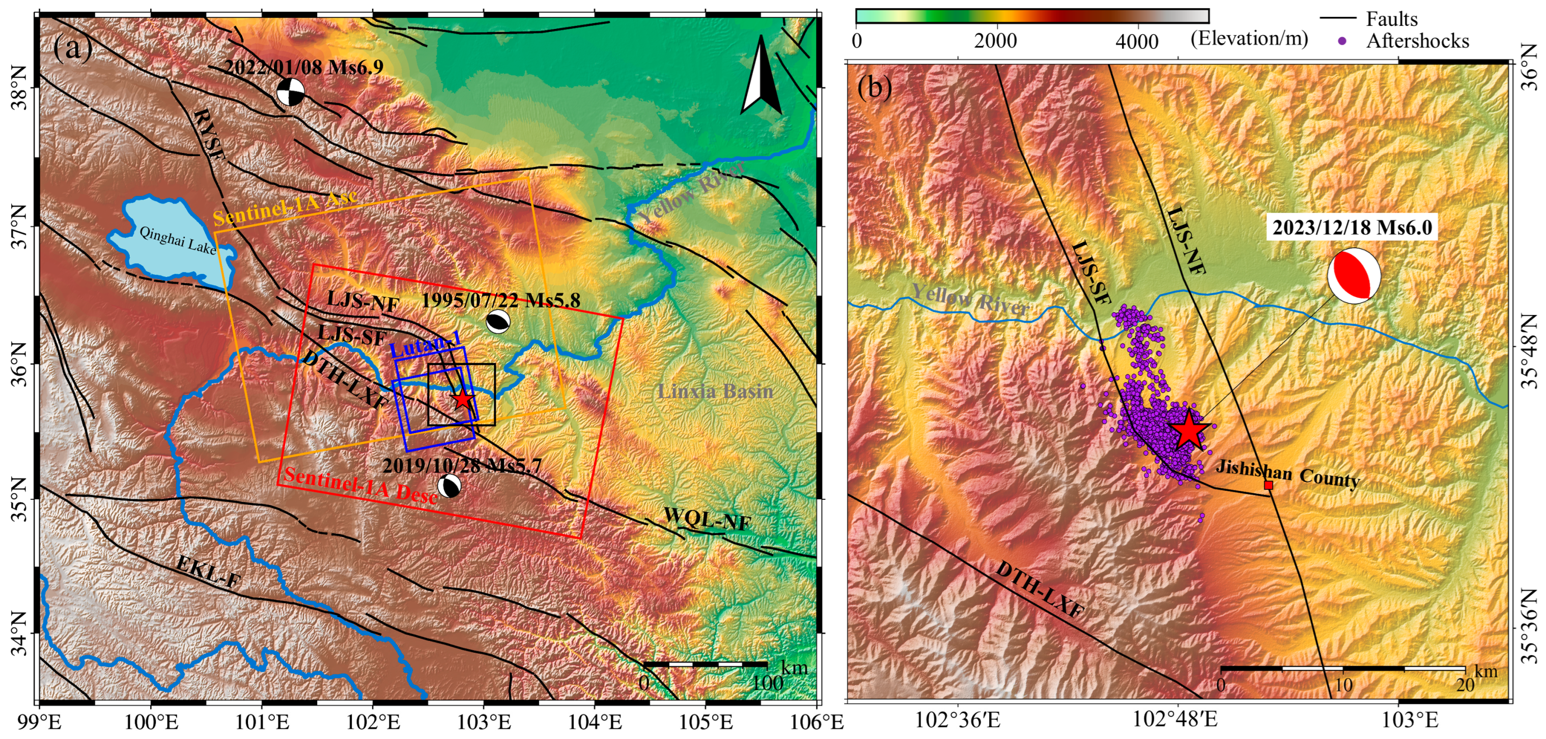
2.2. Summary of the Study Area

The Jishishan earthquake area is located in Jishishan County, Linxia Hui Autonomous Prefecture, Gansu Province, China, in the transition zone between the Tibetan Plateau and the Loess Plateau. The topography of the seismic area gradually decreases from southwest to northeast, and the Yellow River passes through the seismic area from west to east [24,25,26]. In the vicinity of the earthquake area, there is the LJSF, the Daotanghe-Linxia fault (DTH-LXF), the Western Qinling northern margin fault (WQL-NF), and the east Kunlun fault (EFL-F), etc. [27,28,29]. (Figure 1). The LJSF is the main fault zone within the earthquake area, which is mainly an arc-shaped fault that protrudes in the northeast direction, and is an extruded tectonic zone and tectonic transition zone between the left-trending and sliding WQL-NF and the right-trending and sliding Riyueshan fault [30,31,32]. The region is characterized by the development of active ruptures and strong tectonic activities, and earthquakes are frequent. According to records, there have been about 20 earthquakes of moderate intensity of about magnitude 5 in history. For example, the 22 July 1995, Ms5.8 magnitude earthquake in Yongdeng, Gansu, and the 28 October 2019, Ms5.7 magnitude earthquake in Xiahe, Gansu [33] (Figure 1). However, the 2023 Mw6.0 Jishishan earthquake was the largest earthquake that occurred on the LJSF. Therefore, the occurrence of this earthquake provides an important opportunity to use satellite geodetic data to study in-depth the structure and rupture behavior of the subsurface seismogenic faults in the LJS zone region [34].

3. Method and Results

3.1. InSAR Data Processing

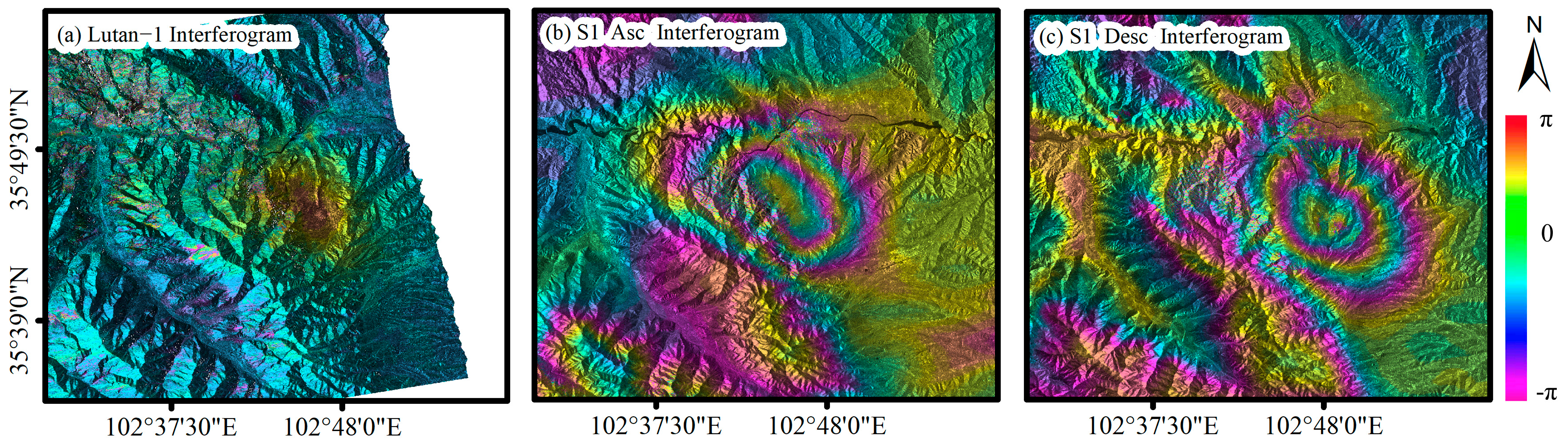
3.1.1. Differential Interferograms with Lutan-1 Data

We used GAMMA software [35] to perform differential interferometric processing on the Lutan-1 data to obtain the differential interferograms (Figure 2) after the Lutan-1 images with two range looks and four azimuth looks, the Sentinel-1A images with 10 range looks and two azimuth looks [36]. As can be seen from Figure 2, there are obvious deformation signals in the differential interferograms of the Lutan-1 and Sentinel-1A data. However, the differential interferograms of the Lutan-1 data do not exhibit obvious interference fringes, in contrast to those of the Sentinel-1A data. This distinction arises from the L-band nature of the Lutan-1 data, with a wavelength of approximately 23 cm. In this context, a displacement change of 11.5 cm in the LOS direction corresponds to one color cycle. Consequently, interference fringes appear in the L-band Lutan-1 data only when the displacement field reaches 11.5 cm. From the differential interferograms of the Sentinel-1A data, we can see that interference fringes experienced about two color cycles, and each color cycle on the Sentinel-1A data represents a 2.8 cm displacement in the LOS direction, which indicates that the displacement of the whole deformation field is about 5.6 cm. Therefore, the displacement field caused by this Jishishan earthquake does not appear as a whole cycle of interference fringes in the differential interferograms of the Lutan-1 data. In addition, there are serious baseline deviations and atmosphere noise in the differential interferograms; they must be corrected to obtain accurate coseismic deformation fields for the subsequent simulation of the seismic source parameters and inversion of the slip distributions, to scientifically evaluate the seismic tectonics and seismicity mechanism of the Jishishan earthquake.

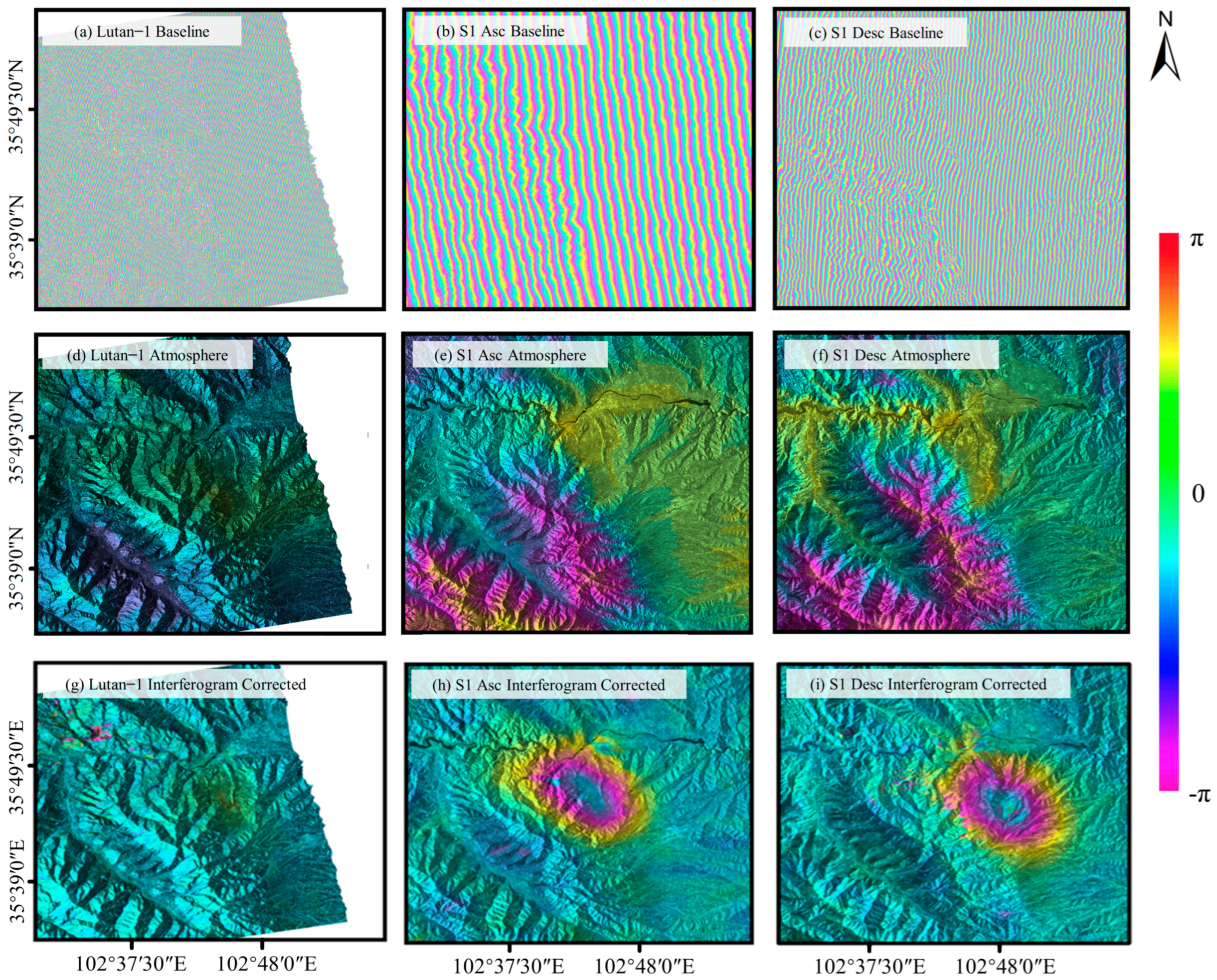
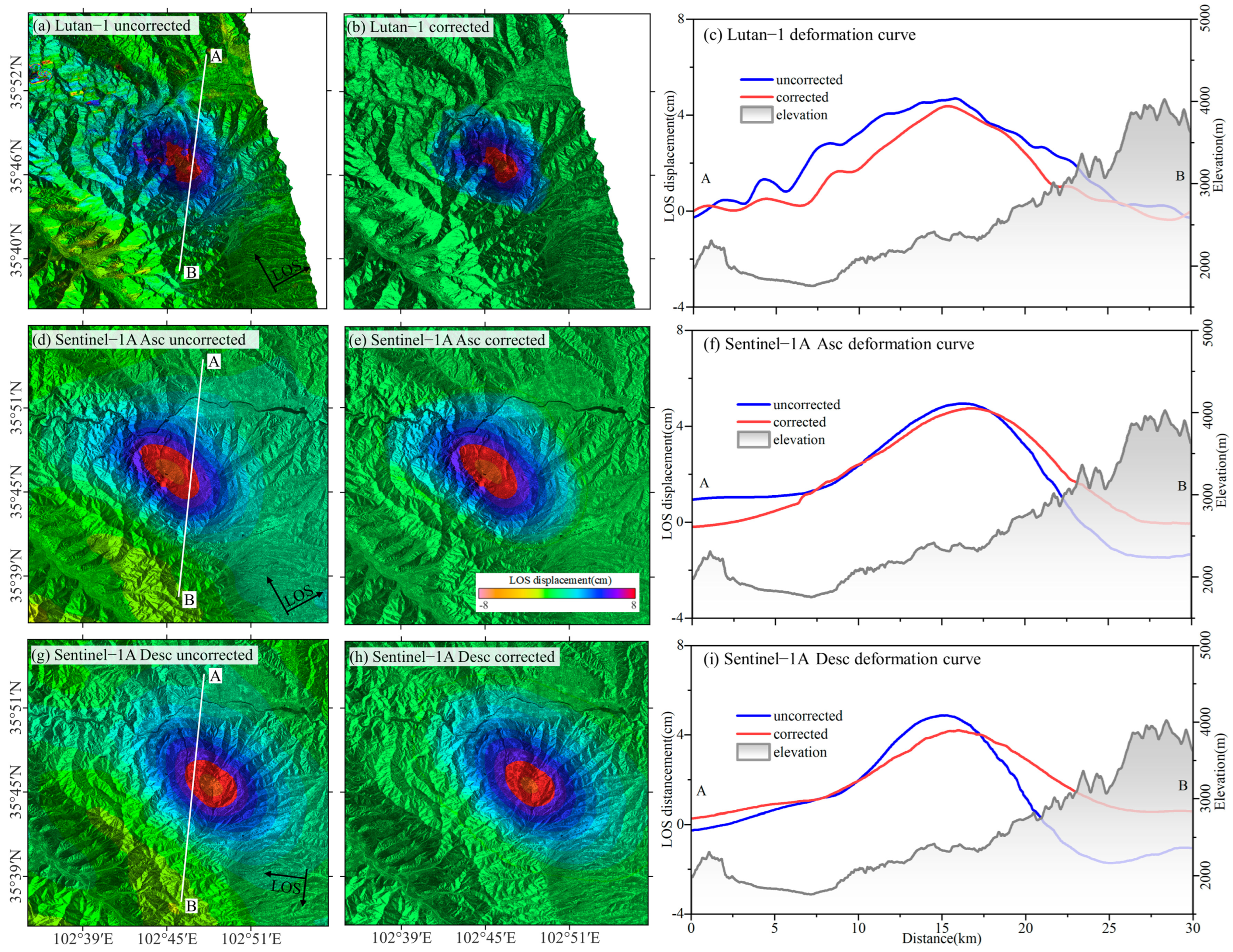
3.1.2. Baseline Deviation and Atmosphere Phase Correction

From the coverage positions of the two Lutan-1 images in Figure 1 and the differential interferograms in Figure 2, we can see that the baseline deviations of the Lutan-1 data are large. Therefore, we weaken the baseline deviation of the Lutan-1 data based on the state vector of Lutan-1 using the least squares model and Fourier analysis [35], resulting in a refined baseline. Then, we remove the effects of terrain phasing using the one-arc second Shuttle Radar Topography Mission (SRTM) DEM [37,38]. It should be noted that the Sentinel-1A satellite is in the progressive scanning (TOPS) mode and the precise orbit data are provided by the European Space Agency (ESA), which has a small baseline deviation. Table 2 shows the initial baseline, improved baseline, and their differences in the Lutan-1 image during Lutan-1 data processing. Figure 3a–c shows the baseline maps for the three data types.
According to Zebker’s research, a 20% change in the water vapor content of the air will result in a 10–14 cm deformation monitoring error [39]. Because of the high elevation and topographic relief in the Jishishan seismic region, we focused on the correction of the vertical atmospheric component associated with elevation changes in the Jishishan seismic region. Wegmuller et al. concluded from their study that the atmospheric phase varies with elevation and exhibits an exponential or linear model relationship [40]. We investigated the relationship between atmospheric phase and elevation in the Jishishan seismic region using Lutan-1 data as an example (Figure 4). The comparison of Figure 4 shows that the R2 value obtained by the exponential model fitting is 0.4605, while the R2 value obtained by the linear model fitting is only 0.3954, and the exponential model fits better than the linear model. Therefore, we utilize an exponential model for atmospheric phase correction in the Jishishan seismic region.
Figure 3 illustrates the process of correcting baseline deviation and atmospheric phase for the three datasets. Figure 3d–f presents the atmospheric phases of these datasets, which have been fitted using an exponential model. The results indicate a strong correlation between atmospheric phases and changes in elevation, suggesting that the exponential model provides a more accurate fit for atmospheric phases. Subsequently, Figure 3g–i displays the differential interferograms following the corrections for baseline deviation and atmospheric effects. When compared to Figure 2, it becomes evident that these corrected differential interferograms offer a more precise representation of coseismic deformation. Consequently, they are better suited for analyzing the coseismic deformation and seismogenic fault.

3.1.3. Coseismic Deformation Fields

We use the minimum cost flow algorithm [35] to phase unwrap regions in the differential interferogram with coherence greater than 0.3. The unwrap phase is transformed into a deformation field and geocoded in World Geodetic System (WGS) 84 coordinates to obtain the final coseismic deformation field. The coseismic deformation fields of the Lutan-1 and Sentinel-1A data are shown in Figure 5. The spatial locations of the coseismic deformation fields of the three types of data are the same, with an elliptical distribution and a long axis extending from northwest to southeast. Moreover, the structure of the coseismic deformation field is relatively single, and the symbols of the coseismic deformation values in the epicenter area are the same, which all show that they are close to the satellite direction from the ground surface, indicating that the deformation is mainly surface uplift, which is in line with the motion characteristics of the thrust fault earthquake. To further analyze the spatial deformation characteristics of the earthquake, we delineated a profile line AB across the coseismic deformation field, as shown in Figure 5a,d,g. Figure 5c,f,i illustrates the variations in LOS displacements along profile AB before and after atmospheric correction, respectively. From Figure 5c,f,i, it can be seen that the coseismic deformation fields of the three data have obvious lifting centers, the maximum value of the LOS-direction displacement reaches about 5 cm, and the displacements between the deformation fields are continuous, and there are no large areas of jumping displacement discontinuities due to excessive deformation gradients, which indicates that the active faults have not ruptured to the surface. The deformation characteristics indicate that the 2023 Mw6.0 Jishishan earthquake exhibited thrust faulting mechanisms, which is consistent with the Global Centroid-Moment-Tensor (GCMT, https://www.Globalcmt.org/, accessed on 20 February 2024) and the United States Geological Survey (USGS, https://earthquake.usgs.gov/earthquakes/, accessed on 20 February 2024).

3.2. Inversion of Seismogenic Fault Parameters

To assess the feasibility of utilizing Lutan-1 data for seismogenic fault parameter inversion, we inverted the source parameters of the 2023 Mw6.0 Jishishan earthquake using both uniform slip and distributed slip models [41] based on Lutan-1 data, and compared the results with those derived from Sentinel-1 data inversion.

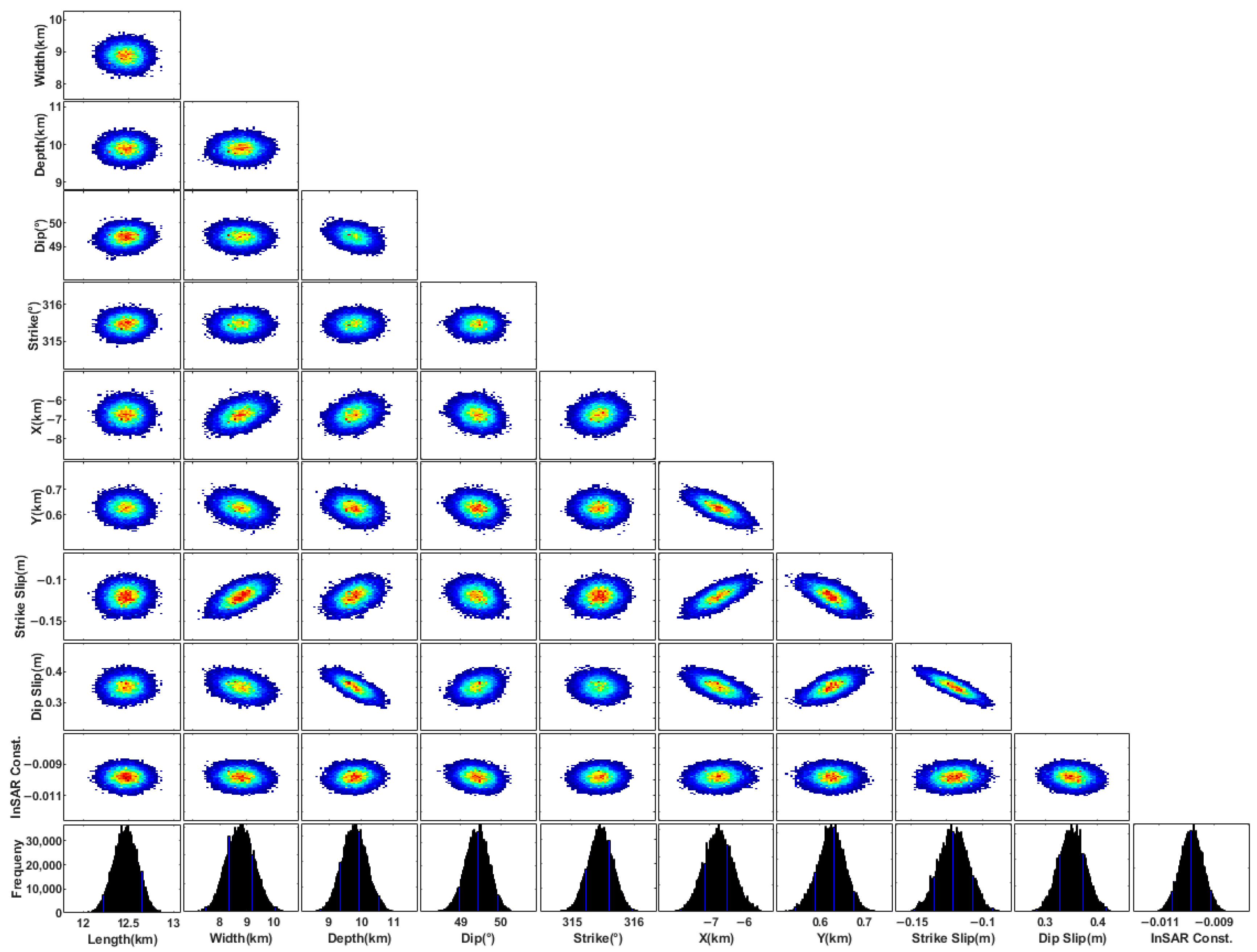
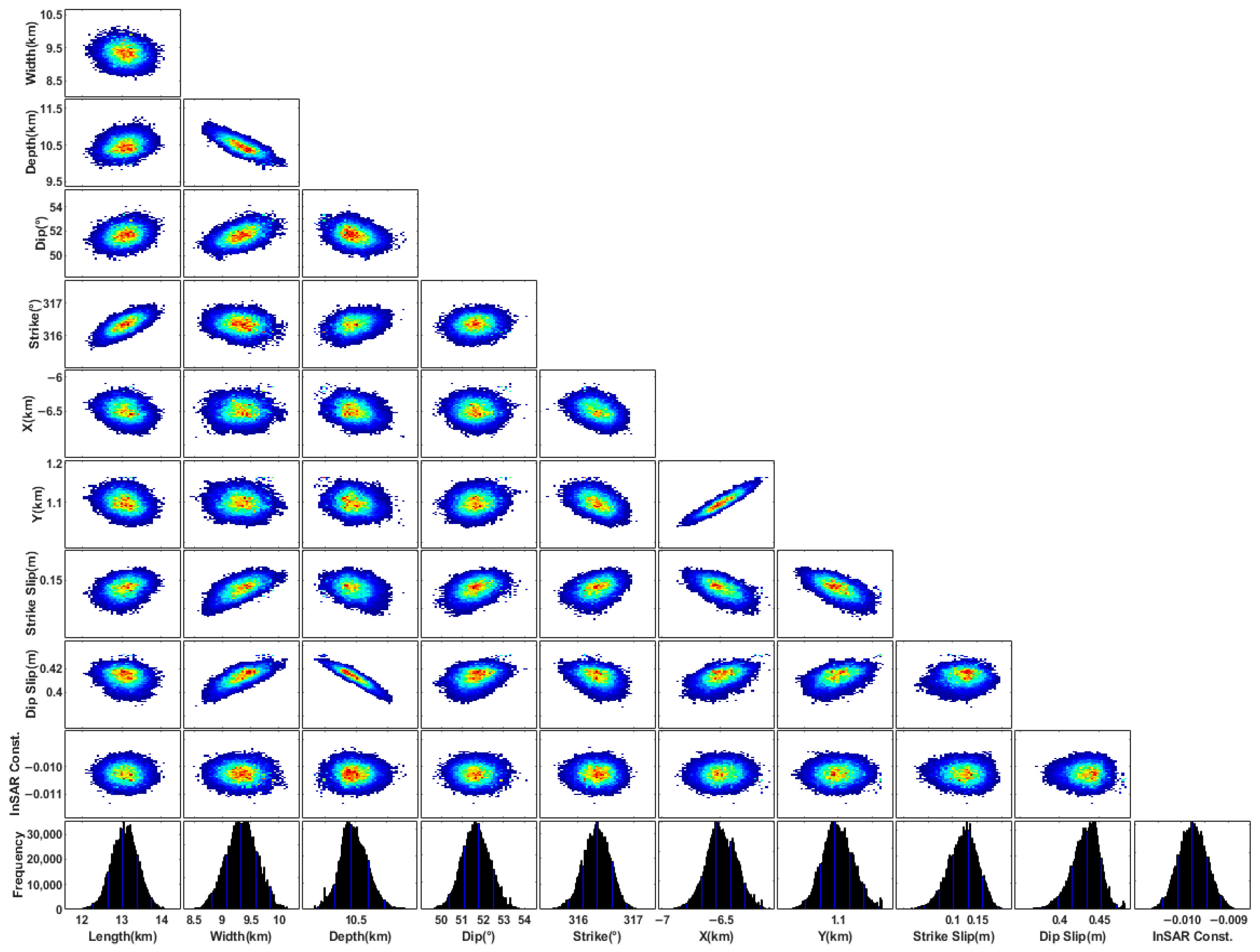
3.2.1. Uniform Slip Modeling

We implemented the inversion process for a uniform slip model using a MATLAB(Version 2021b)-based geodetic Bayesian inversion software (GBIS) [41,42]. First, to mitigate the influence of noise and improve computational efficiency, the coseismic deformation field was downsampled using an adaptive quadtree algorithm, with a downsampling threshold set to 1 × 10⁻⁴. Next, the spatial variability of the coseismic deformation field was calculated using a semi-variogram, and its trend component was removed by fitting a theoretical exponential function. Finally, the uniform slip model was iterated 106 times, with the ranges and step sizes of the fault parameters during the inversion process set, as shown in Table 3. These values play a critical role in the inversion of fault parameters. It should be noted that the same steps were applied to the inversion of Sentinel-1A data, with only minor differences in parameter settings.
The inversion results of the uniform slip model using Lutan-1 data are presented in Table 4 and Figure 6. Table 4 shows the 95% confidence intervals of the seismogenic fault parameter inverted from Lutan-1 data. Figure 6 displays the joint probability density distributions of the source parameters. As shown in Table 4 and Figure 6, the coseismic surface displacements can be effectively explained by a fault with a length of 10.89 km to 14.15 km, a width of 7.51 km to 11.14 km, a strike of 312.95° to 317.69°, and a dip angle of 48.12° to 50.47°. The slip direction is consistent with a thrust fault, with a smaller left-lateral component. The slip amounts in the two directions range from −0.15 m to 0.17 m and 0.28 m to 0.46 m, respectively. The optimal length, width, and depth of the thrust fault are 12.67 km, 9.25 km, and 10.14 km, respectively, with a dip angle and strike of 49.36° and 315.38°. These results demonstrate the feasibility of using Lutan-1 data for fault parameter inversion.
Table 4 also presents the inversion results derived from Sentinel-1 data, along with the seismogenic fault parameter provided by other seismic research institutions. Figure 7 shows the joint probability density distribution based on Sentinel-1 data. By comparing the inversion results from different studies, as well as Figure 6 and Figure 7, it can be observed that the seismogenic fault parameter inverted from Lutan-1 data exhibits good consistency with those obtained from Sentinel-1 data and those reported by institutions such as USGS and GCMT, although minor differences exist. These discrepancies can be attributed to variations in the InSAR coseismic deformation fields and differences in parameter settings, as both the coseismic deformation field and parameter configurations are critical for fault parameter inversion. However, these slight differences in the inverted parameters do not affect the main conclusion that Lutan-1 data can serve as a reliable tool for seismogenic fault inversion analysis.

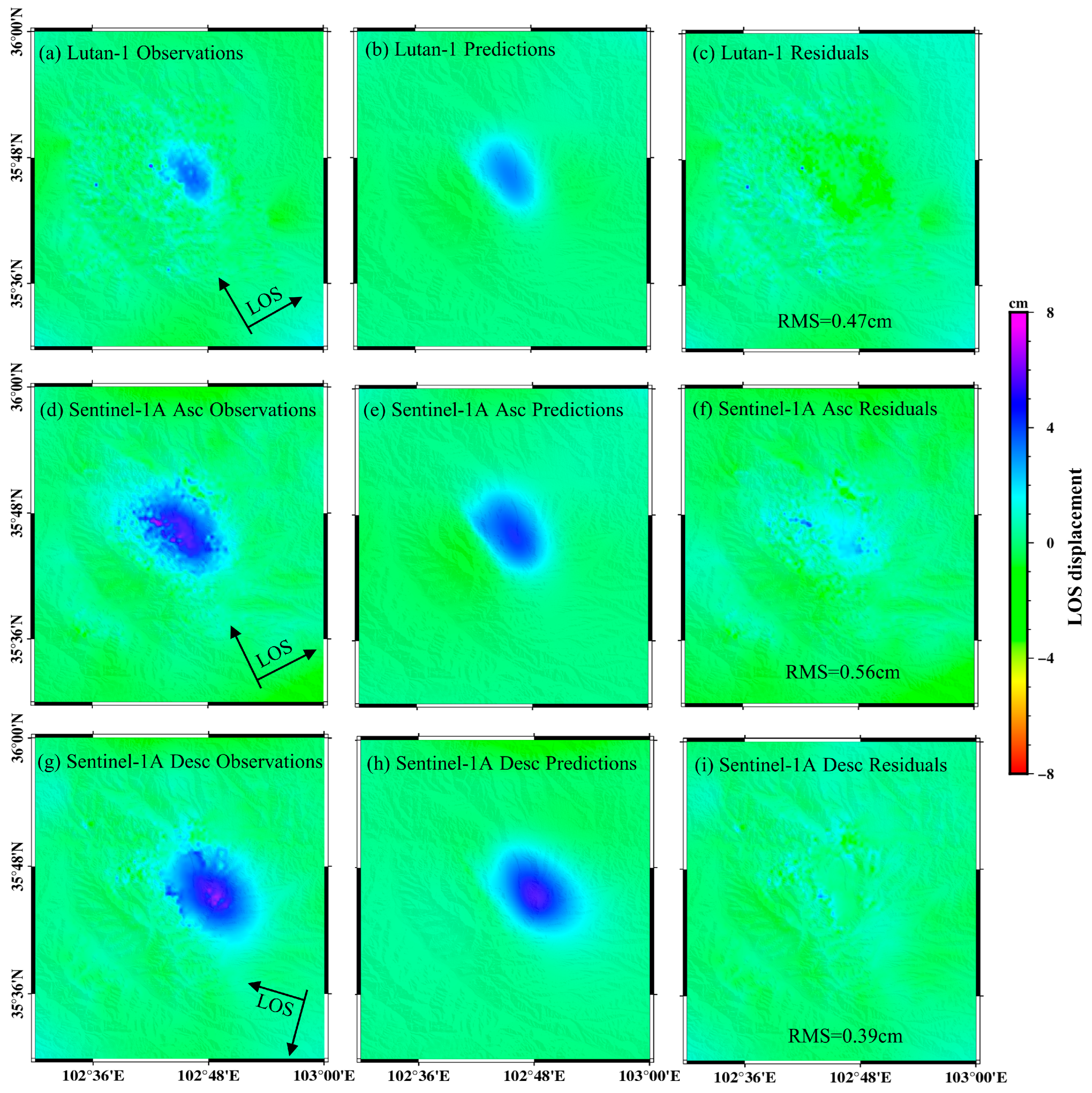
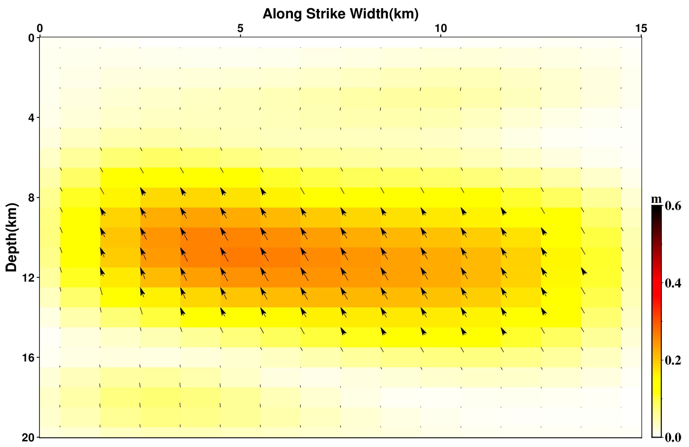
3.2.2. Distributed Slip Modeling

On the basis of utilizing a uniform slip model for the inversion of seismogenic fault parameters, we employed the Steepest Descent Method (SDM) [43,44] to perform the inversion for a distributed slip model. Furthermore, to distinguish it from the uniform slip model, we independently inverted the ascending and descending data of Sentinel-1A using the distributed slip model and compared the inversion results from the three datasets. To mitigate potential boundary effects during the inversion process, we appropriately extended the length (along strike) and width (along dip) of the rectangular fault plane, simulating the earthquake as a 15 km × 20 km rectangular dislocation, discretized into 300 subfaults of 1 km × 1 km each. Given the relatively low sensitivity of the uniform slip model to fault dip angles, the distributed slip inversion process was researched for dip angles within the range of [35°, 70°] (with a search step of 1°). Additionally, a smoothing factor was introduced to reduce the influence of unstable factors during the inversion, with the smoothing factor searched within the range of [0.01, 1.5] (with a search step of 0.05). Finally, under the constraints of the optimal dip angle (51°) and smoothing coefficient (0.07), the slip distribution on the fault plane of this earthquake was obtained. The inversion results based on Lutan-1 and Sentinel-1A data are shown in Figure 8. It can be observed that the observed results from Lutan-1 data exhibit excellent consistency with the inversion results, with a root mean square (RMS) error of only 0.47 cm. Moreover, the inversion results from Lutan-1 and Sentinel-1A data also demonstrate good consistency, indicating the feasibility of inverting seismogenic fault parameters using the distributed slip model based on Lutan-1 data.
Based on the inversion results derived from Lutan-1 data, the fault slip distribution of the 2023 Mw6.0 Jishishan earthquake was obtained, as illustrated in Figure 9. It is observed that the 2023 Mw6.0 Jishishan earthquake exhibits a minor right-lateral strike-slip component, with its coseismic slip not rupturing to the surface. The majority of the slip is concentrated at depths between 8 and 14 km. The maximum slip amount of 0.27 m occurs at a depth of 10.3 km below the surface, releasing a seismic moment of 1.01 × 10¹⁸ N·m, corresponding to an Mw6.0 magnitude earthquake. This result is consistent with findings from institutions such as GCMT, USGS, and GFZ, demonstrating the validity of the slip distribution derived from Lutan-1 data and confirming the capability of Lutan-1 data for inverting seismic slip distributions.

4. Discussion

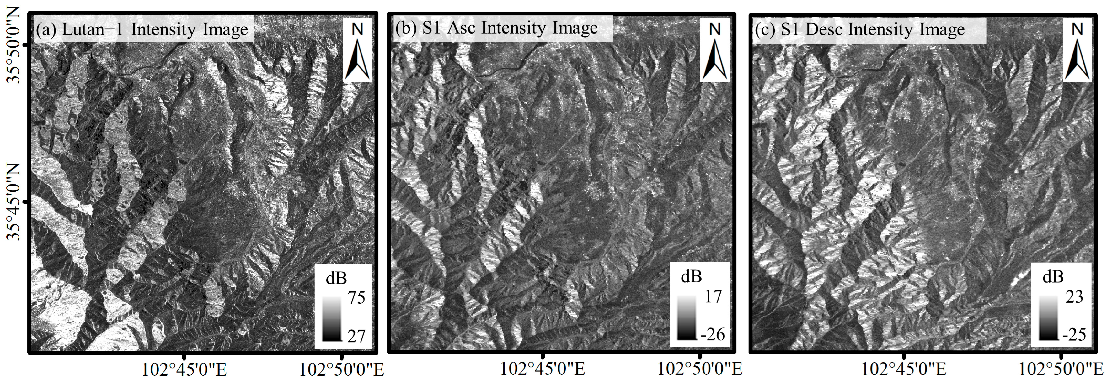
4.1. Comparative Analysis of SAR Intensity Images

In the field of InSAR, the dB (decibel) value is utilized to represent the intensity of radar signals, thereby reflecting the quality of radar imagery. The relationship between the dB value and intensity is expressed by the following formula [45]:
dB = 10 log 10 I
where I represents the intensity of the radar image. As can be inferred from the above formula, a high dB value typically indicates strong signal strength and high quality of the SAR image. Conversely, a negative dB value signifies an intensity value of less than 1.
Figure 10 displays the intensity images of Lutan-1 and Sentinel-1 following the earthquake. It is observed that the dB values of the coseismic deformation field from Lutan-1 data range from 27 to 75, whereas the dB values of Sentinel-1 ascending data range only from −26 to 17, and those of the descending data range from −25 to 23. Notably, all pixel dB values from Lutan-1 data are higher than those from the corresponding Sentinel-1 data. This indicates that the quality of Lutan-1 data is significantly superior to that of Sentinel-1 data, providing enhanced intensity information.

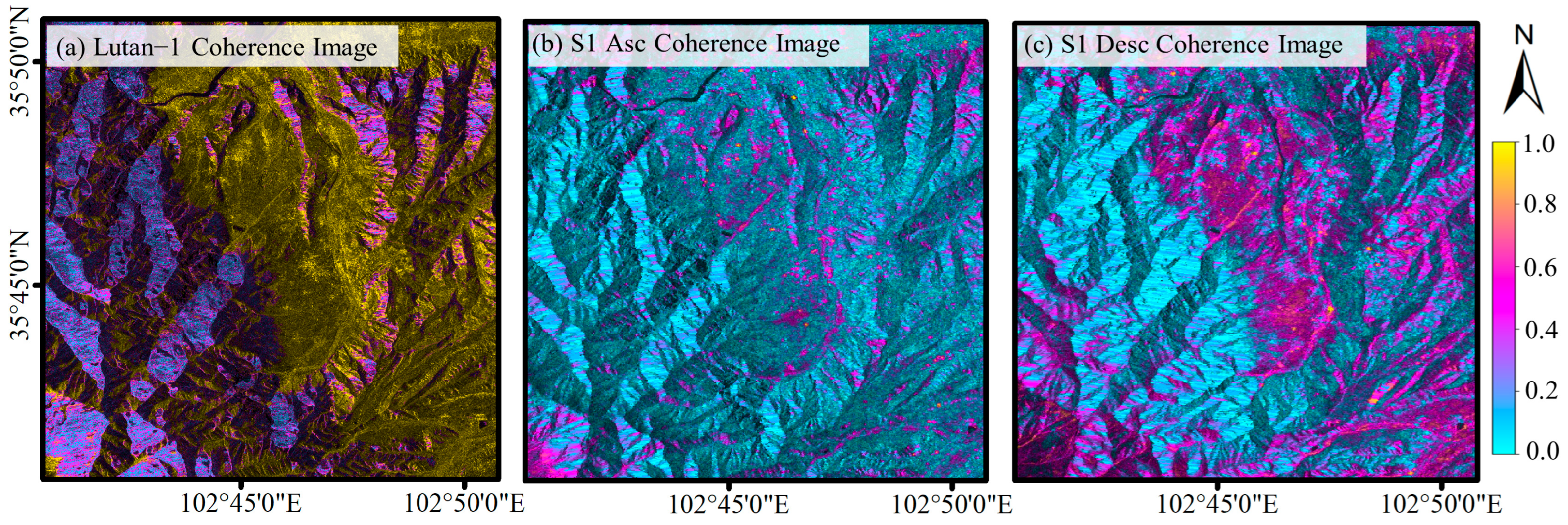
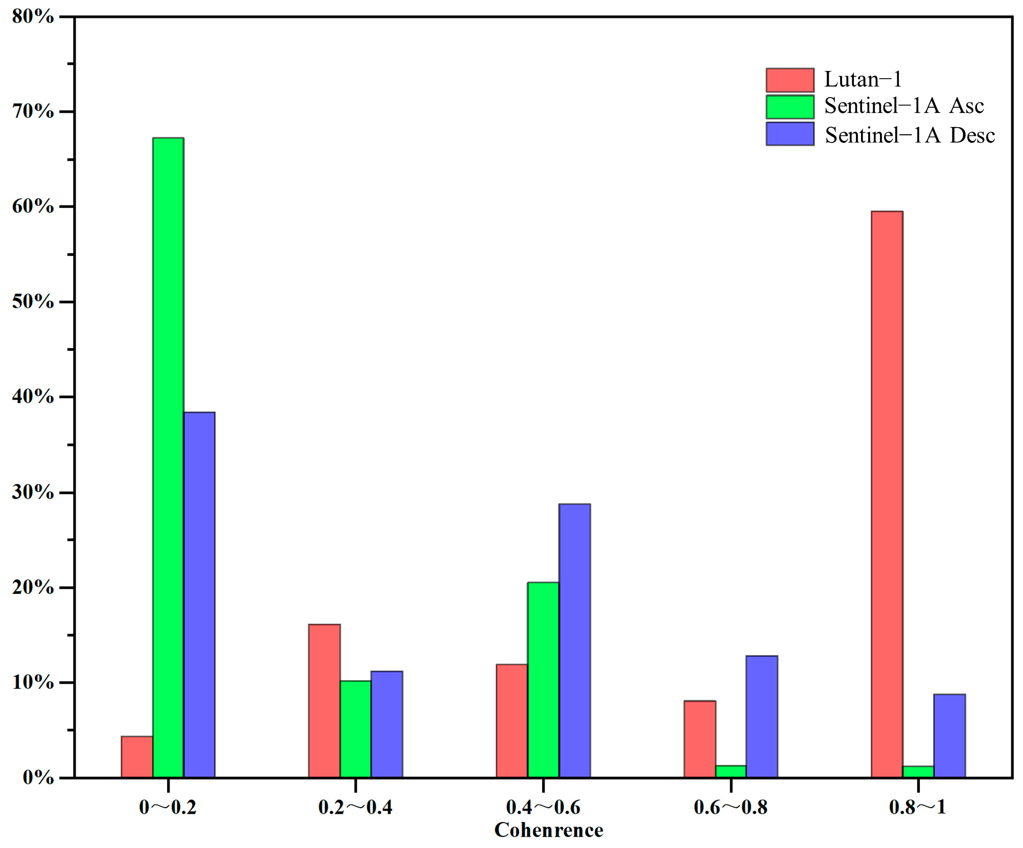
4.2. Comparative Analysis of Coherence

To further evaluate the interferometric performance of Lutan-1 data, a comparison of coherence among the three datasets was conducted. Figure 11 presents the coherence images of the coseismic deformation field, clearly illustrating that Lutan-1 data exhibit significantly better coherence in the coseismic deformation field compared to Sentinel-1A data. For a more precise comparison of the interferometric performance of the three datasets, coherence was categorized into five intervals: (0~0.2], (0.2~0.4], (0.4~0.6], (0.6~0.8], and (0.8~1.0]. Table 5 summarizes the number of pixels in each coherence interval, and Figure 12 displays the proportion of each coherence interval. Combining Table 5 and Figure 12, it is evident that the peak coherence interval for Lutan-1 data lies within 0.8~1.0, whereas the peak coherence intervals for Sentinel-1A ascending and descending data are 0~0.2. Defining pixels with coherence greater than 0.6 as highly coherent, Lutan-1 data cover 68% of the highly coherent regions in the coseismic deformation field, while Sentinel-1A ascending and descending data cover only 3% and 22%, respectively. This demonstrates that Lutan-1 data provide superior interferometric performance compared to Sentinel-1A data, offering a clearer depiction of surface changes in the coseismic deformation field.

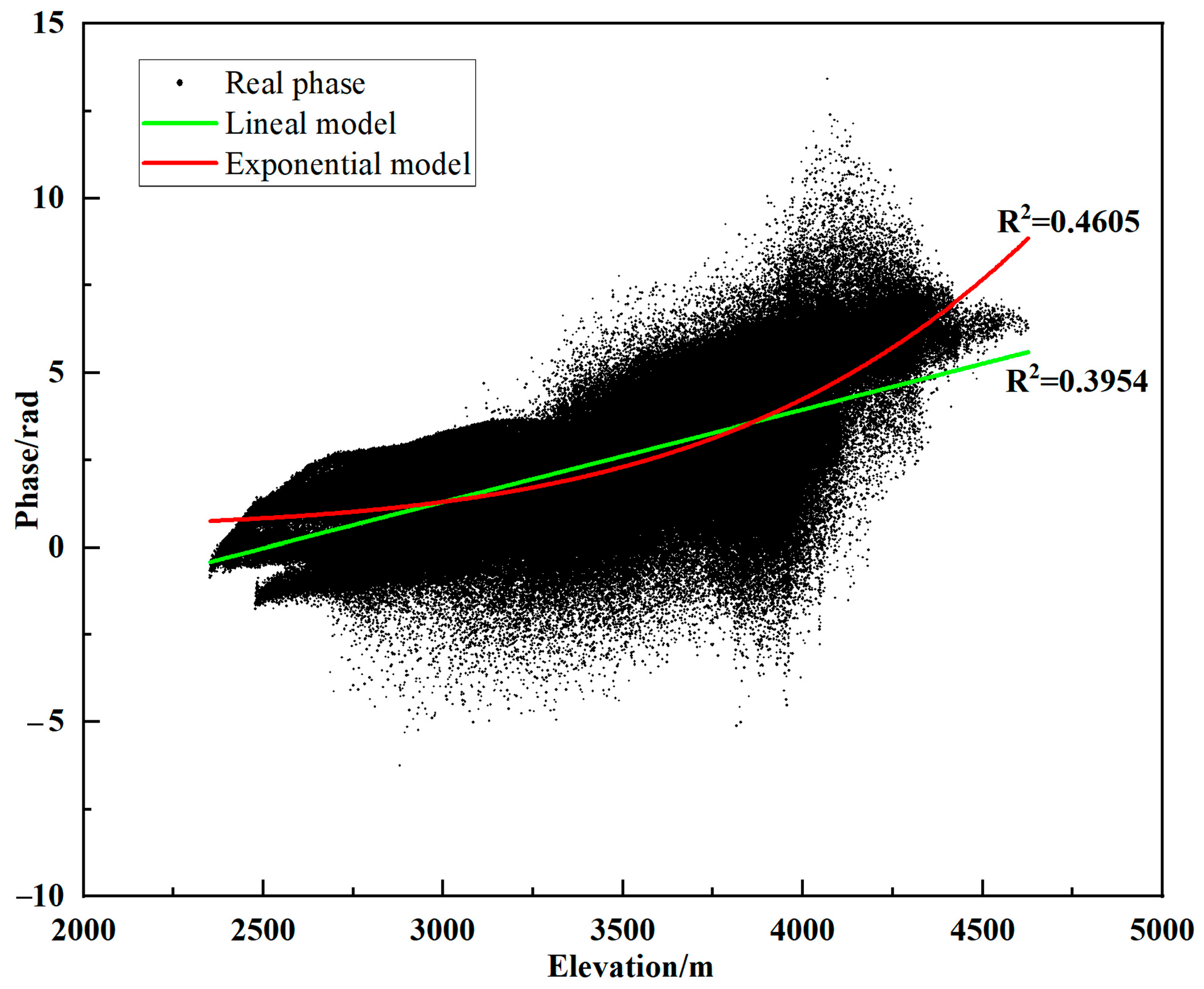
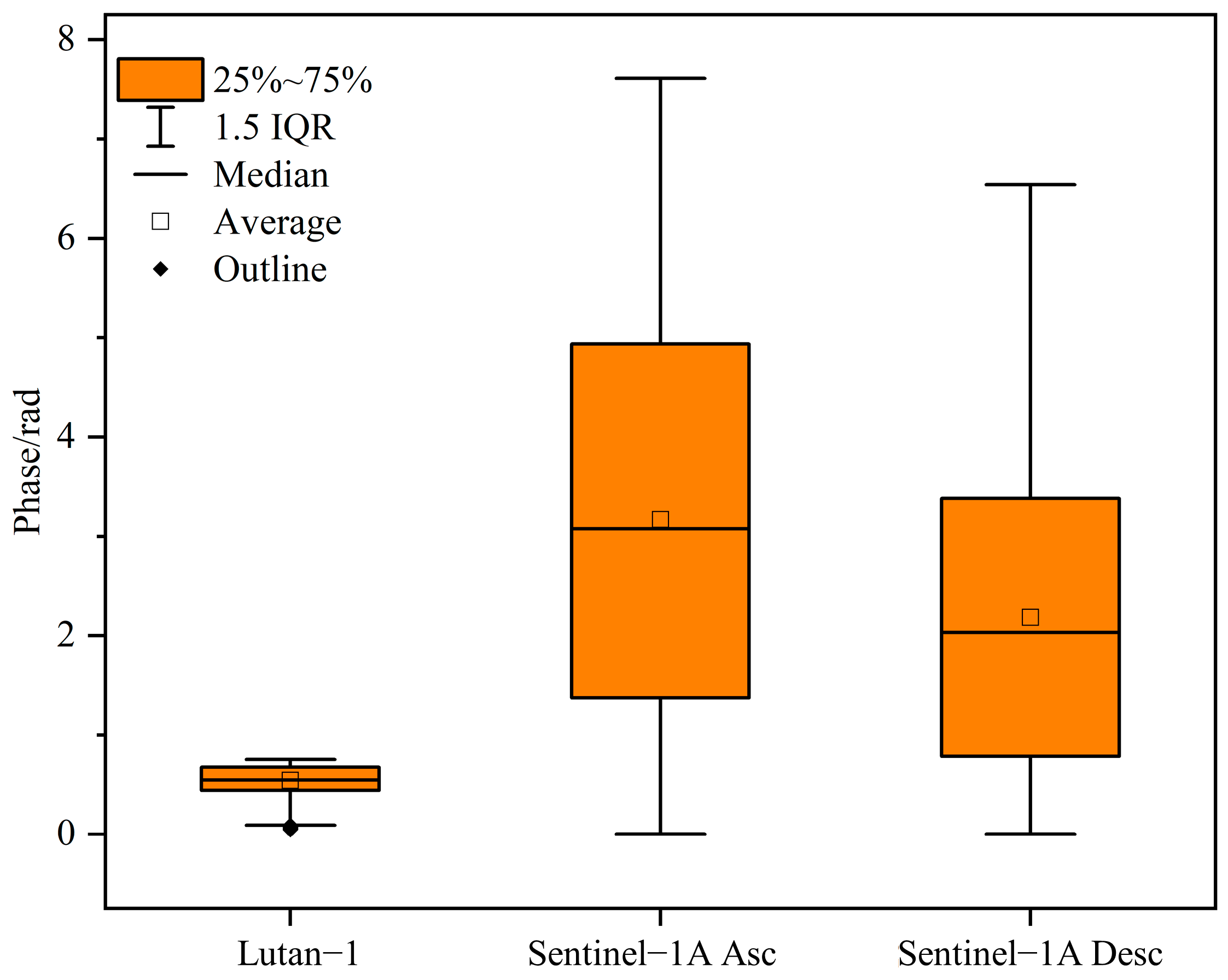
4.3. Comparative Analysis of Atmospheric Phase

This section presents a quantitative analysis of atmospheric phases from Lutan-1 and Sentinel-1A data within the seismic region. To avoid ambiguity, we calculated and displayed the absolute values of atmospheric phases from all three datasets in Figure 13. Overall, the Lutan-1 data exhibits a more concentrated atmospheric phase distribution, suggesting less atmospheric interference and greater stability. The proximity between mean and median values indicates a symmetrical distribution pattern. The Sentinel-1A data exhibit a broader distribution of atmospheric phase values, and the mean value is slightly higher than the median, indicating the data stability is relatively poor and that atmospheric interference is heightened. Specifically, the maximum atmospheric phase of the Lutan-1 data is 0.75 rad (equivalent to ~1.4 cm displacement), and the average atmospheric phase is about 0.5 rad (~9 mm displacement). Sentinel-1A ascending data have an atmospheric phase maximum of 7.61 rad (~3.4 cm displacement) and an average atmospheric phase of ~3.2 rad (~1.4 cm displacement), while descending data exhibit a maximum phase of 6.5 rad (~2.9 cm displacement) and an average of ~2.3 rad (~1 cm displacement). The above comparison shows that the maximum and average values of the atmospheric phases of Lutan-1 data are lower than those of Sentinel-1A data, indicating that the atmospheric effects in the Jishishan seismic region interfere less with the Lutan-1 data, which is because the L-band Lutan-1 data penetrate the atmosphere more easily and are less sensitive to atmospheric factors such as humidity and cloud cover. Therefore, when selecting InSAR data for surface deformation monitoring, Lutan-1 data should be given priority.
In addition, we also found that the measurement errors caused by the atmospheric phase values of both the Lutan-1 data and the Sentinel-1A data reach the centimeter level, which can cause serious interference to the analysis of the coseismic deformation and seismogenic fault analysis, and thus atmospheric correction of the coseismic deformation field is very necessary.

4.4. Comparative Analysis of Coseismic Deformation Field

The coseismic deformation field obtained by Lutan-1 is about 12 km × 9 km (Figure 5b), while the Sentinel-1A ascending and descending data (Figure 5e,h) is about 14 km × 11 km. After analyzing the data, we identified the following factors contributing to the discrepancies between the coseismic deformation fields observed in the Lutan-1 and Sentinel-1A data: (1) the angle of incidence of the Lutan-1 data is 22.49°, whereas the Sentinel-1A ascending and descending data have incidence angles of 40.70° and 41.57°, respectively. The disparity in incidence angles between the Lutan-1 data and the Sentinel-1A ascending and descending data are substantial, with differences in −18.21° and −19.08°, respectively. The ratios of the LOS directional displacements for Lutan-1 and Sentinel-1A ascending and descending data are calculated as sin 22.49° (sin 40.7°)−1 = 0.587 and sin 22.49° (sin 41.57°)−1 = 0.576, both of which are below 0.6. It is a key factor contributing to the disparities in the range of the coseismic deformation field and deformation displacements between the Lutan-1 and Sentinel-1A data; (2) the Jishishan earthquake is a mainshock–aftershock type earthquake. The post-earthquake Lutan-1 data were collected on 22 December 2023, while the Sentinel-1A data were collected on 26 December 2023, resulting in a 4-day difference between the two sets of satellite data. According to the aftershock location catalog of the Jishishan earthquake released by the China Earthquake Administration (https://www.cea.gov.cn/cea/dzpd/dzzt/d138bc8c-1.html, accessed on 20 February 2024) and Fang Lihua’s team (http://esdc.ac.cn/article/149, accessed on 20 February 2024), 142 aftershocks occurred between 22 December and 26 December, of which the number of aftershocks of magnitude 1 or higher was 11, with the largest aftershock (magnitude 3.0) occurring on 22 December at 14:43 (the Lutan-1 data were collected on 22 December at 10:57). For the Jishishan earthquake area, which had just experienced a magnitude 6.0 earthquake, the soft soil and disrupted geological structures may lead to changes in the deformation field due to the 142 aftershocks. This is also a potential contributing factor.

5. Conclusions

In this paper, we initially utilized Lutan-1 data to obtain the coseismic deformation field of the 2023 Mw 6.0 Jishishan earthquake. Subsequently, we inverted the seismogenic fault parameters and slip distribution of the earthquake based on the InSAR deformation monitoring results derived from Lutan-1 data. Finally, we conducted a comparative analysis between the Lutan-1 data and Sentinel-1A data. This study provides a theoretical foundation for the application of Lutan-1 data in earthquake hazard research, with specific conclusions as follows: (1) The coseismic deformation monitoring and seismogenic fault parameters inversion results derived from Lutan-1 and Sentinel-1 data are generally consistent, demonstrating the capability of Lutan-1 data for coseismic deformation monitoring and seismogenic fault parameters inversion; (2) Compared to Sentinel-1A data, Lutan-1 data exhibits superior visibility in the coseismic deformation zone, accompanied by higher coherence and lower atmospheric noise, demonstrating the advantages of Lutan-1 data for earthquake monitoring; (3) The 2023 Mw 6.0 Jishishan earthquake was a thrust-type event, characterized primarily by uplift in its coseismic deformation field. The slip distribution was concentrated at depths ranging from 8 to 14 km, with a maximum slip of 0.27 m occurring at a depth of 10.3 km below the surface. The seismic moment released was 1.01 × 10¹⁸ N·m, corresponding to an earthquake of Mw 6.0 magnitude.

Author Contributions

All the authors participated in editing and reviewing the manuscript. Conceptualization, X.L. and J.P.; methodology, X.L.; validation, X.L., X.M. and M.S.; investigation, X.L., X.J. and C.W.; data curation, X.L. and Y.Z.; writing—original draft preparation, X.L.; writing—review and editing, X.L., J.P., Y.Z., X.C., Y.P., Y.S. and X.Q.; visualization, X.L.; supervision, J.P.; project administration, J.P.; funding acquisition, J.P. All authors have read and agreed to the published version of the manuscript.

Funding

This research was funded by the National Natural Science Foundation of China under Grant 42074004.

Data Availability Statement

The Sentinel-1 images were freely available through the Alaska Satellite Facility (https://search.asf.alaska.edu/; accessed on 30 December 2024). The focal mechanism of the 2023 Mw6.0 Jishishan earthquake was accessed from https://www.cea-igp.ac.cn/kydt/280418.html (accessed on 22 December 2023). The black focal mechanisms were obtained from the USGS (https://earthquake.usgs.gov/earthquakes/; accessed on 5 February 2024).

Acknowledgments

The authors are grateful to Wenyu Gong of the Institute of Geology, China Earthquake Administration, for her valuable suggestions on the structure and writing of this paper, and the Land Satellite Remote Sensing Application Center of the Ministry of Natural Resources and the Airborne Geophysical Exploration Remote Sensing Center of the China Geological Survey provide Lutan-1 data.

Conflicts of Interest

The authors declare no conflicts of interest.

References

  1. Li, M.; Wang, Y.; Li, W.; Jiang, K.; Zhang, Y.; Lyu, H.; Zhao, Q. Performance evaluation of real-time orbit determination for LUTAN-01B satellite using broadcast earth orientation parameters and multi-GNSS combination. GPS Solut. 2023, 28, 52. [Google Scholar] [CrossRef]
  2. Zhang, Y.; Li, Y.; Chen, Z.; Zhao, X.; Liu, Y.; Hu, C. First Result of Lutan-1 Space-Surface Bistatic SAR Interferometry. In Proceedings of the IGARSS 2023—2023 IEEE International Geoscience and Remote Sensing Symposium, Pasadena, CA, USA, 17–21 July 2023; pp. 7860–7863. [Google Scholar]
  3. Deng, Y.; Wang, Y. Key technologies for spaceborne SAR payload of LuTan-1 satellite system. Acta Geod. Cartogr. Sin. 2024, 53, 1881–1895. [Google Scholar]
  4. Mou, J.; Wang, Y.; Hong, J.; Wang, Y.; Wang, A.; Sun, S.; Liu, G. First Assessment of Bistatic Geometric Calibration and Geolocation Accuracy of Innovative Spaceborne Synthetic Aperture Radar LuTan-1. Remote Sens. 2023, 15, 5280. [Google Scholar] [CrossRef]
  5. Ji, Y.; Zhang, X.; Li, T.; Fan, H.; Xu, Y.; Li, P.; Tian, Z. Mining Deformation Monitoring Based on Lutan-1 Monostatic and Bistatic Data. Remote Sens. 2023, 15, 5668. [Google Scholar] [CrossRef]
  6. Wang, R.; Liu, K.; Liu, D.; Ou, N.; Yue, H.; Chen, Y.; Yu, W.; Liang, D.; Cai, Y. LuTan-1: An innovative L-band spaceborne bistatic interferometric synthetic aperture radar mission. IEEE Geosci. Remote Sens. Mag. 2025, 2–22. [Google Scholar] [CrossRef]
  7. Liu, B.; Zhang, L. Application of InSAR Monitoring Large Deformation of Landslides Using Lutan-1 Constellation. Geomat. Inf. Sci. Wuhan Univ. 2024, 49, 1753–1762. [Google Scholar]
  8. Yu, Z.; Yan, L. Research and application of Lutan-1 SAR satellite in survey andmonitoring of catastrophic geohazards. Bull. Surv. Mapp. 2024, 11, 97–101. [Google Scholar]
  9. Li, T.; Tang, X.; Zhou, X.; Zhang, X.; Li, S.; Gao, X. Deformation Products Of Lutan-1(Lt-1) Sar Satellite Constellation for Geohazard Monitoring. In Proceedings of the IGARSS 2022—2022 IEEE International Geoscience and Remote Sensing Symposium, Kuala Lumpur, Malaysia, 17–22 July 2022; pp. 7543–7546. [Google Scholar]
  10. Xu, B.; Liu, L.; Li, Z.; Zhu, Y.; Hou, J.; Mao, W. Design Bistatic Interferometric DEM Generation Algorithm and Its Theoretical Accuracy Analysis for LuTan-1 Satellites. J. Geod. Geoinf. Sci. 2022, 5, 25–38. [Google Scholar]
  11. Li, Y.; Liu, H.; Yang, C. Revisiting the seismic hazards of faults surrounding the 2022 Ms6.8 Luding earthquake, Sichuan, China. Geomat. Nat. Hazards Risk 2023, 14, 2272569. [Google Scholar] [CrossRef]
  12. Zhang, Y.; Zhang, G.; Hetland, E.A.; Shan, X.; Zhang, H.; Zhao, D.; Gong, W.; Qu, C. Source Fault and Slip Distribution of the 2017 Mw 6.5 Jiuzhaigou, China, Earthquake and Its Tectonic Implications. Seismol. Res. Lett. 2018, 89, 1345–1353. [Google Scholar] [CrossRef]
  13. Daoyang, Y.; Peizhen, Z. A preliminary study on the new activity features of the Lajishan mountain fault zone in Qinhai Province. Earthq. Res. 2005, 32, 93–102. [Google Scholar]
  14. Zhang, Z.; Zeng, Q.; Jiao, J. Deformations monitoring in complicated-surface areas by adaptive distributed Scatterer InSAR combined with land cover: Taking the Jiaju landslide in Danba, China as an example. ISPRS J. Photogramm. Remote Sens. 2022, 186, 102–122. [Google Scholar] [CrossRef]
  15. Su, Y.; Peng, J.; Shi, M.; Guo, C.; Ma, X.; Li, X.; Wang, J.; Wang, W. An M-Estimation Method for InSAR Nonlinear Deformation Modeling and Inversion. IEEE Trans. Geosci. Remote Sens. 2024, 62, 5207912. [Google Scholar] [CrossRef]
  16. Zhu, C.H.; Wang, C.S.; Zhang, B.C.; Qin, X.Q.; Shan, X.J. Differential Interferometric Synthetic Aperture Radar data for more accurate earthquake catalogs. Remote Sens. Environ. 2021, 266, 112690. [Google Scholar] [CrossRef]
  17. Morishita, Y. A Systematic Study of Synthetic Aperture Radar Interferograms Produced From ALOS-2 Data for Large Global Earthquakes From 2014 to 2016. IEEE J. Sel. Top. Appl. Earth Obs. Remote Sens. 2019, 12, 2397–2408. [Google Scholar] [CrossRef]
  18. Zhou, Y.; Zhou, C.; E, D.; Wang, Z. A Baseline-Combination Method for Precise Estimation of Ice Motion in Antarctica. IEEE Trans. Geosci. Remote Sens. 2014, 52, 5790–5797. [Google Scholar] [CrossRef]
  19. Ma, X.; Peng, J.; Su, Y.; Shi, M.; Zheng, Y.; Li, X.; Jiang, X. Deformation Characteristics and Activation Dynamics of the Xiaomojiu Landslide in the Upper Jinsha River Basin Revealed by Multi-Track InSAR Analysis. Remote Sens. 2024, 16, 1940. [Google Scholar] [CrossRef]
  20. Zheng, Y.; Peng, J.; Chen, X.; Huang, C.; Chen, P.; Li, S.; Su, Y. Spatial and Temporal Evolution of Ground Subsidence in the Beijing Plain Area Using Long Time Series Interferometry. IEEE J. Sel. Top. Appl. Earth Obs. Remote Sens. 2023, 16, 153–165. [Google Scholar] [CrossRef]
  21. Huang, X.; Li, Y.; Shan, X.; Zhong, M.; Wang, X.; Gao, Z. Fault Kinematics of the 2023 Mw 6.0 Jishishan Earthquake, China, Characterized by Interferometric Synthetic Aperture Radar Observations. Remote Sens. 2024, 16, 1746. [Google Scholar] [CrossRef]
  22. Liu, Z.; Bingquan, H.; Yihan, N.; Zhenhong, L.; Chen, Y.; Chuang, S.; Bo, C.; Lijiang, Z.; Xuesong, Z.; Jianbing, P. Source Parameters and Slip Distribution of the 2023 Mw 6.0 Jishishan (Gansu, China) Earthquake Constrained by InSAR Observations. Geomat. Inf. Sci. Wuhan Univ. 2025, 50, 344–355. [Google Scholar] [CrossRef]
  23. Fang, N.; Kai, S.; Chuanchao, H.; Chengyuan, B.; Zhidan, C.; Lei, X.; Zhi, Y.; Yinghui, X.; Hongbin, X.; Guangcai, F.; et al. Joint Inversion of InSAR and Seismic Data for the Kinematic Rupture Process of the 2023 Ms 6.2 Jishishan Earthquake. Geomat. Inf. Sci. Wuhan Univ. 2025, 50, 333–343. [Google Scholar] [CrossRef]
  24. Lease, R.O.; Burbank, D.W.; Clark, M.K.; Farley, K.A.; Zheng, D.; Zhang, H. Middle Miocene reorganization of deformation along the northeastern Tibetan Plateau. Geology 2011, 39, 359–362. [Google Scholar] [CrossRef]
  25. Wang, M.; Shen, Z.K. Present-Day Crustal Deformation of Continental China Derived From GPS and Its Tectonic Implications. J. Geophys. Res. Solid Earth 2020, 125, e2019JB018774. [Google Scholar] [CrossRef]
  26. Daoyang, Y.; Peizhen, Z. Late Cenozoic tectonic deformation of the Linxia Basin, northeastern margin of the Qinghai-Tibet Plateau. Earth Sci. Front. 2007, 14, 243–250. [Google Scholar]
  27. Zheng, D.; Peizhen, Z. Tectonic events, climate and conglom erate: Example from Jishishan and mountain and Linxia basin. Quat. Sci 2006, 26, 63–69. [Google Scholar]
  28. Li, M.; Gao, Y. Basic Characteristics of Tectonics and Seismie Anisotropy inthe Southeastern Margin of the Qinghai-Tibet Plateau. Earthquake 2021, 41, 15–45. [Google Scholar]
  29. Bai, Y.; Ni, H. Advances in Research on the Geohazard Effect of Active Faults on the Southeastern Margin of the Tibetan Plateau. J. Geomech. 2019, 25, 1116–1128. [Google Scholar]
  30. Saylor, J.E.; Jordan, J.C.; Sundell, K.E.; Wang, X.; Wang, S.; Deng, T. Topographic growth of the Jishi Shan and its impact on basin and hydrology evolution, NE Tibetan Plateau. Basin Res. 2017, 30, 544–563. [Google Scholar] [CrossRef]
  31. Zhuang, W.; Cui, D.; Hao, M.; Song, S.; Li, Z. Geodetic constraints on contemporary three-dimensional crustal deformation in the Laji Shan–Jishi Shan tectonic belt. Geod. Geodyn. 2023, 14, 589–596. [Google Scholar] [CrossRef]
  32. Peizhen, Z.; Daoyang, Y. Discussion on late Cenozoic growth and rise of northeastern margin of the Tibetan Plateau. Quat. Sci. 2006, 26, 5–13. [Google Scholar]
  33. Bai, Z.; Ji, L.; Zhu, L.; Chen, H.; Xu, C.; Bian, Z.; Wang, J. Study on the process and mechanism of slip-mudflow in Zhongchuan Township induced by the Jishishan earthquake in 2023. China Earthq. Eng. J. 2024, 46, 768–777. [Google Scholar] [CrossRef]
  34. Wang, X.; Flynn, L.J.; Deng, C. A review of the Cenozoic biostratigraphy, geochronology, and vertebrate paleontology of the Linxia Basin, China, and its implications for the tectonic and environmental evolution of the northeastern margin of the Tibetan Plateau. Palaeogeogr. Palaeoclimatol. Palaeoecol. 2023, 628, 111775. [Google Scholar] [CrossRef]
  35. Werner, C.; Wegmüller, U.; Strozzi, T.; Wiesmann, A. GAMMA SAR and Interferometric Processing Software. In Proceedings of the ERS-Envisat Symposium, Gothenburg, Sweden, 16–20 October 2000. [Google Scholar]
  36. Scheiber, R.; Bothale, V.M. Interferometric Multi-look Techniques for SAR Data. In Proceedings of the IEEE International Geoscience and Remote Sensing Symposium, Toronto, ON, Canada, 24–28 June 2002; pp. 173–175. [Google Scholar]
  37. Wright, T.J. Remote monitoring of the earthquake cycle using satellite radar interferometry. Philos. Trans. R. Soc. A Math. Phys. Eng. Sci. 2002, 360, 2873–2888. [Google Scholar] [CrossRef] [PubMed]
  38. Massonnet, D.; Feigl, K.L. Radar interferometry and its application to changes in the Earth’s surface. Rev. Geophys. 1998, 36, 441–500. [Google Scholar] [CrossRef]
  39. Zebker, H.A.; Rosen, P.A.; Hensley, S. Atmospheric effects in interferometric synthetic aperture radar surface deformation and topographic maps. J. Geophys. Res. Solid Earth 1997, 102, 7547–7563. [Google Scholar] [CrossRef]
  40. Wegmuller, U.; Walter, D.; Spreckels, V.; Werner, C.L. Nonuniform Ground Motion Monitoring With TerraSAR-X Persistent Scatterer Interferometry. IEEE Trans. Geosci. Remote Sens. 2010, 48, 895–904. [Google Scholar] [CrossRef]
  41. Okada, Y. Surface Deformation Due to Shear and Tensile Faults in a Half-Space. Bull. Seismol. Soc. Am. 1985, 75, 1135–1154. [Google Scholar] [CrossRef]
  42. Bagnardi, M.; Hooper, A. Inversion of Surface Deformation Data for Rapid Estimates of Source Parameters and Uncertainties: A Bayesian Approach. Geochem. Geophys. Geosyst. 2018, 19, 2194–2211. [Google Scholar] [CrossRef]
  43. Rongjiang, W.; Diao, F.; Hoechner, A. SDM—A geodetic inversion code incorporating with layered crust structure and curved fault geometry. In Proceedings of the EGU General Assembly Conference, Vienna, Austria, 7–12 April 2013; Volume 15. [Google Scholar]
  44. Wang, R.; Lorenzo-Martín, F.; Roth, F. PSGRN/PSCMP—A new code for calculating co- and post-seismic deformation, geoid and gravity changes based on the viscoelastic-gravitational dislocation theory. Comput. Geosci. 2006, 32, 527–541. [Google Scholar] [CrossRef]
  45. Feng, S.; Dai, K.; Sun, T.; Deng, J.; Tang, G.; Han, Y.; Ren, W.; Sang, X.; Zhang, C.; Wang, H. Mini-Satellite Fucheng 1 SAR: Interferometry to Monitor Mining-Induced Subsidence and Comparative Analysis with Sentinel-1. Remote Sens. 2024, 16, 3457. [Google Scholar] [CrossRef]
Figure 1. Tectonic setting and SAR image coverage of the Jishishan earthquake. (a) The black rectangle indicates the magnified tectonic setting of the epicenter area. The black beach ball indicates historical earthquakes, and the red pentagram indicates the epicenter location of the Jishishan earthquake. (b) The purple circle shows the aftershock sequence of the Jishishan earthquake (Historical earthquake information and source mechanism solution from USGS). RYSF: Riyueshan fault; LJS-NF: Lajishan northern margin fault; LJS-SF: Lajishan southern margin fault; DTH-LXF: Daotanghe–Linxia fault; WQL-NF: Western Qinling northern margin fault; EKL-F: Eastern Kunlung fault.
Remotesensing 17 00894 g001
Figure 2. Differential interferograms of Lutan-1 (a), Sentinel-1A ascending (b) and descending data (c).
Remotesensing 17 00894 g002
Figure 3. Baseline deviation and atmospheric phase correction process of Lutan-1, Sentinel-1A ascending and descending data. (ac) are the baseline images; (df) are the atmospheric phase distributions Images; (gi) are the corrected differential interferograms.
Remotesensing 17 00894 g003
Figure 4. Relationship between atmospheric phase and elevation in the seismic zone of Jishishan for Lutan-1 data.
Remotesensing 17 00894 g004
Figure 5. Coseismic deformation fields for Lutan-1, Sentinel-1A ascending and descending data. (a,d,g) are before Atmospheric Correction; (b,e,h) are after Atmospheric Correction; (c,f,i) are the LOS Deformation Curves of the AB Profile.
Remotesensing 17 00894 g005
Figure 6. Joint probability density distribution of Seismogenic fault parameters for Lutan-1 data. The figure is generated based on frequency, with cool colors for low frequency, warm colors for high frequency.
Remotesensing 17 00894 g006
Figure 7. Joint probability density distribution of Seismogenic fault parameters for Sentinel-1A data. The figure is generated based on frequency, with cool colors for low frequency, warm colors for high frequency.
Remotesensing 17 00894 g007
Figure 8. Distributed slip model of the 2023 Mw6.0 Jishishan earthquake for Lutan-1, Sentinel-1A ascending and descending data. (a,d,g) are InSAR observations results; (b,e,h) are predictions results; (c,f,i) are the residuals between the observations and predictions results.
Remotesensing 17 00894 g008
Figure 9. 2023 Mw6.0 Jishishan earthquake seismic fault coseismic slip distribution map based on Lutan-1; the arrows indicate the direction of slip.
Remotesensing 17 00894 g009
Figure 10. SAR intensity images of Lutan-1 (a), Sentinel-1A ascending (b), and descending data (c).
Remotesensing 17 00894 g010
Figure 11. Coherence Images of Lutan-1 (a), Sentinel-1A ascending (b) and descending data (c).
Remotesensing 17 00894 g011
Figure 12. Coherence distribution of Lutan-1 (a), Sentinel-1A ascending (b), and descending data (c).
Remotesensing 17 00894 g012
Figure 13. Atmospheric phase statistics for three data types in the Jishishan seismic region.
Remotesensing 17 00894 g013
Table 1. Main parameters of the SAR data in this study.
SAR SensorLutan-1Sentinel-1ASentinel-1A
Path 128135
Orbital directionAscendingAscendingDescending
Reference date18 December 202327 October 202314 December 2023
Secondary date22 December 202326 December 202326 December 2023
Time baseline (day)46012
B (m)740.1564.30114.60
Wavelength (cm)235.65.6
Incidence (°)22.4941.5639.17
Heading (°)348.63−13.12193.12
Pixel spacing (Range × Azimuth) (m)1.67 × 1.742.33 × 13.942.33 × 13.94
Image wide (km)50250250
ModeStripmapTOPSTOPS
Table 2. Baseline of Lutan-1 data.
SAR SensorsBaselineBc (m)Bn (m) B c r a t e (m/s) B n r a t e (m/s)
Lutan-1Initial baseline719.796−188.033−0.887−0.092
Precise baseline717.589−187.211−0.848−0.141
Baseline deviation−2.2070.8220.039−0.049
Table 3. Seismogenic fault parameters and step size settings for the uniform slip model.
Length (km)Width (km)Depth (km)Dip (°)Strike (°)X 1 (km)Y 1 (km)Strike Slip (m)Dip Slip (m)
Lower0.5100200−10−10−5−5
Upper50502589.9360101055
Step0.050.050.05110.10.10.010.01
1 X and Y denote the deviation of the midpoint of the upper boundary of the fault from the reference point.
Table 4. Seismogenic fault parameters of the 2023 Mw6.0 Jishishan earthquake.
Source Length (km)Width (km)Depth (km)Dip (°)Strike (°)X
(km)
Y
(km)
Strike Slip (m)Dip Slip (m)Mw
Lutan-1Optimal12.679.2510.1449.36315.38−7.120.66−0.130.356.0
2.5%10.897.519.0548.12312.95−7.84−0.18−0.150.28
97.5%14.1511.1411.3250.47317.69−6.331.350.170.46
Sentinel-1AOptimal13.129.3710.7751.76316.54−6.571.130.120.416.0
2.5%11.398.679.6849.75314.41−7.290.45−0.060.24
97.5%14.5210.5811.8353.52320.72−6.021.760.310.58
USGSOptimal--1062333----5.9
GCMTOptimal--18.952331----6.1
Huang et al. [21]Optimal13.1610.9615.0355.9320.418.4712.68−0.010.326.0
Liu et al. [22]Optimal1489.343319----6.0
Fang et al. [23]Optimal12.967.965.5432.2325.2−6.452.870.1−0.2496.2
Table 5. Number of pixels in different coherence intervals.
Source0~0.20.2~0.40.4~0.60.6~0.80.8~1.0
Lutan-139,388147,158108,77373,579542,682
Sentinel-1A Asc613,90993,115187,32411,73711,126
Sentinel-1A Desc350,481102,417262,473116,73680,028
Disclaimer/Publisher’s Note: The statements, opinions and data contained in all publications are solely those of the individual author(s) and contributor(s) and not of MDPI and/or the editor(s). MDPI and/or the editor(s) disclaim responsibility for any injury to people or property resulting from any ideas, methods, instructions or products referred to in the content.

