Assessment of the Impacts of Different Carbon Sources and Sinks on Atmospheric CO₂ Concentrations Based on GEOS-Chem

Abstract

Global atmospheric CO₂ concentrations, driven by anthropogenic emissions and natural carbon cycle dynamics, have emerged as a critical accelerator of climate change. However, due to the spatiotemporal heterogeneity of carbon sources and sinks, estimating CO₂ flux remains highly uncertain. Accurately quantifying the contribution of various carbon sources and sinks to atmospheric CO₂ concentration is essential for understanding the carbon cycle and global carbon balance. In this study, GEOS-Chem (version 13.2.1), driven by MERRA-2 meteorological data, was used to simulate monthly global CO₂ concentrations from 2006 to 2010. The model was configured with a horizontal resolution of 2.5° longitude × 2.0° latitude and 47 vertical hybrid-sigma layers up to 0.01 hPa. To evaluate the impact of different emission sources and sinks, the “Inventory switching and replacing” approach was applied, designing a series of numerical experiments in which individual emission sources were selectively disabled. The contributions of eight major CO₂ flux components, including fossil fuel combustion, biomass burning, balanced biosphere, net land exchange, aviation, shipping, ocean exchange, and chemical sources, were quantified by comparing the baseline simulation (BASE) with source-specific perturbation experiments (no_X). The results show that global CO₂ concentration exhibits a spatial pattern with higher concentrations in the Northern Hemisphere and land areas, with East Asia, Southeast Asia, and eastern North America being high-concentration regions. The global average CO₂ concentration increased by 1.8 ppm year⁻¹ from 2006 to 2010, with China’s eastern region experiencing the highest growth rate of 3.0 ppm year⁻¹. Fossil fuel combustion is identified as the largest CO₂ emission source, followed by biomass burning, while oceans and land serve as significant CO₂ sinks. The impact of carbon flux on atmospheric CO₂ concentration is primarily determined by the spatial distribution of emissions, with higher flux intensities in industrialized and biomass-burning regions leading to more pronounced local concentration increases. Conversely, areas with strong carbon sinks, such as forests and oceans, exhibit lower net CO₂ accumulation.

1. Introduction

Global warming has become one of the most pressing environmental challenges facing the world today. The dramatic increase in atmospheric carbon dioxide (CO₂) concentration is widely considered one of the primary drivers of climate change. According to the Annual Greenhouse Gas Index (AGGI) report from the National Oceanic and Atmospheric Administration (NOAA), the total radiative forcing of global greenhouse gases increased by 49% from 1990 to 2023, with CO₂ accounting for approximately 80% of this increase. In 2023, the global annual average CO₂ concentration reached 419.3 ± 0.1 ppm, representing a 51% increase relative to pre-industrial levels. Furthermore, the annual CO₂ growth rate was 2.8 ± 0.01 ppm·year⁻¹, a slight increase compared to the previous year [1]. The continued rise in CO₂ concentration has exacerbated global warming and placed immense pressure on the global climate system, making it a central driving force of climate change.

Changes in atmospheric CO₂ concentration are influenced not only by anthropogenic carbon emissions but also by natural carbon cycles. The global carbon budget is a key regulatory factor in the variability of atmospheric CO₂ concentration, with carbon sources (such as fossil fuel combustion and biomass burning) and carbon sinks (such as terrestrial and oceanic carbon absorption) jointly controlling CO₂ emissions and absorption [1]. However, due to the spatial distribution, temporal variability, and assessment methods of both carbon sources and sinks, there is considerable uncertainty in CO₂ flux estimates, which presents a significant challenge for accurately predicting atmospheric CO₂ concentrations. Previous studies have shown that global carbon flux estimates can vary significantly due to differences in emission inventories, transport models, and observational constraints. For instance, the study by Peylin et al. (2013) [2] found that global CO₂ flux estimates can differ by as much as 10–15% based on variations in emission inventories, particularly between national inventory-based and consumption-based approaches. Additionally, the TransCom intercomparison study reported that discrepancies among 17 different transport models could lead to variations of up to 30% in regional CO₂ flux estimates, mainly due to differences in atmospheric transport process representations and model resolutions [3]. Carbon sources and sinks exhibit significant spatiotemporal heterogeneity, with their emissions characterized by randomness, seasonality, broad distribution, and difficulties in monitoring. Understanding the precise spatiotemporal variations of these carbon sources and sinks and quantifying their impacts on atmospheric CO₂ concentration is of great scientific importance and practical value for addressing climate change and formulating effective carbon emission control policies.

To study the spatiotemporal changes in atmospheric CO₂ concentration, scientists widely use atmospheric chemical transport models. These models simulate variations in meteorological data and source–sink fluxes, effectively reflecting the dynamic characteristics of CO₂ concentration in the atmosphere [4]. Among these models, GEOS-Chem, a global three-dimensional chemical transport model, has been extensively applied in both forward simulations and inversion analyses, significantly improving the estimation of surface carbon fluxes [5,6]. Studies have shown that GEOS-Chem successfully reproduces observed CO₂ variations and it has been used to investigate the impacts of biospheric processes and climate anomalies on atmospheric CO₂ concentrations [7]. The reliability of model simulations depends on observational validation. Ground-based, airborne, and satellite observations are commonly used to assess the accuracy of CO₂ simulations. For instance, Feng et al. (2011) [8] combined ground and satellite observational data from 2003 to 2006 to assess the performance of the global chemical transport model GEOS-Chem in simulating CO₂. Additionally, NOAA’s Carbon Tracker system represents a data assimilation approach, which integrates observational data with transport models to improve CO₂ flux estimates and has been notably successful in optimizing global carbon flux estimates [9]. However, such approaches remain sensitive to transport model biases. Discrepancies among multiple transport models, as found in the TransCom intercomparison study, can lead to considerable variations in CO₂ flux estimates [3].

In the GEOS-Chem atmospheric chemical transport model, the variation in CO₂ concentration is driven by various carbon sources and sinks and is regulated by atmospheric transport processes. Existing studies show that emission sources, such as fossil fuel combustion, biomass burning, and biofuel use, contribute significantly to CO₂ concentration, with considerable spatial variability in their emissions [10]. On the carbon sink side, the absorption of CO₂ by terrestrial ecosystems and oceans plays a crucial role in regulating atmospheric CO₂ levels. Through simulation analysis, researchers have found that fossil fuel combustion is the largest global CO₂ emission source, while the flux variations in the biosphere are the main cause of seasonal fluctuations in atmospheric CO₂ concentrations [11]. Nassar et al. (2010) demonstrated that aviation and maritime emissions significantly increase the latitudinal gradient of global CO₂ concentrations, whereas the impact of chemical sources is relatively minor [12]. Furthermore, oceanic and terrestrial carbon exchanges play a significant role in mitigating the rise in atmospheric CO₂ concentrations [13].

Although numerous studies have explored the role of individual carbon sources or sinks, most have focused on the effects of major carbon sources and sinks such as fossil fuel combustion and terrestrial carbon fluxes, with relatively few examining the integrated effects of multiple carbon flux components on atmospheric CO₂ and the interrelationships among them [2]. This study, based on the GEOS-Chem atmospheric chemical transport model, simulates the global atmospheric CO₂ concentrations from 2006 to 2010, analyzes the spatial distribution and temporal variations of CO₂ concentrations, and validates the model using NOAA-ESRL ground-based observation data and GOSAT satellite data to assess its accuracy. Additionally, through a series of numerical experiments, this study investigates the impacts of eight major CO₂ sources and sinks (fossil fuel combustion, biomass burning, balanced biosphere, net land exchange, maritime, aviation, oceanic exchange, and chemical sources) on global atmospheric CO₂ concentration variations. By comparing the results, this study reveals the contribution differences in various CO₂ sources and sinks to atmospheric CO₂ concentration changes in different regions of the world. This research will provide new insights into understanding the mechanisms of atmospheric CO₂ variation in the global carbon cycle and offer scientific support for the accurate validation of global carbon emission inventories and the formulation of climate policies.

2. Date and Methods

2.1. GEOS-Chem Model Description

The continuously improving 3-D atmospheric chemical transport model GEOS-Chem describes atmospheric transmission, diffusion, reaction, and elimination on local to global scales. The GEOS-Chem model’s CO₂ simulation module, originally developed by Suntharalingam et al. (2003, 2004) [10,14] underwent substantial upgrades through Nassar et al.’s work. GEOS-Chem Classic version 13.2.1 was used for the global CO₂ concentration simulations. The model grid was selected with a horizontal resolution of 2.5° longitude × 2.0° latitude and 47 vertical hybrid-sigma layers up to 0.01 hPa. The simulations were driven by the Modern-Era Retrospective Analysis for Research and Applications, Version 2 (MERRA-2) meteorological fields from the Goddard Earth Observing System (GEOS) of the NASA Global Modeling and Assimilation Office (GMAO) [15]. CO₂ was transported as a tracer in the model with prescribed prior CO₂ fluxes. These included biomass burning emission, fossil fuel emission, ocean exchange emission, balanced biosphere exchange, net terrestrial exchange, ship emission, aviation emission, and CO₂ chemical sources from the oxidation of atmospheric carbon species such as carbon monoxide (CO), methane (CH₂), and non-methane volatile organic compounds (NMVOCs) (

Table 1. List of CO₂ emission inventories used in the GEOS-Chem simulations in this study.

Flux Type	Inventory Name Abbreviation	Description	Spatial	Temporal	References
Biomass Burning	QFED	Quick Fire Emissions Database for 2006–2010	0.1° × 0.1°	Daily	[16]
Fossil Fuel	ODIAC	Open-source Data Inventory for Atmospheric CO2 for 2006–2010	1° × 1°	Monthly	[17]
Ocean Exchange	Scaled ocean exchange	Scaled ocean exchange for 2006–2010	4° × 5°	Monthly	[18]
Balanced Biosphere	SIB3	Balanced Net Ecosystem Production (NEP) CO2 for 2006–2010	1° × 1.25°	3-hourly	[19]
Net Terrestrial Exchange	TransCom climatology	TransCom net terrestrial biospheric CO2 fixed in 2000	1° × 1°	Fixed	[20]
Ship	CEDS	Community Emissions Data System for 2006–2010	0.5° × 0.5°	Monthly	[21]
Aviation	AEIC	Aircraft Emissions Inventory Code fixed in 2005	1° × 1°	Monthly	[22]
Chemical Source	CO2 Chemical Source	CO2 chemical production from carbon species oxidation fixed in 2004	2° × 2.5°	Monthly	[12]

).

2.2. Numerical Experiments

A uniform initial global average CO₂ concentration value of 373.71 ppm was set for 1 January 2003, based on the annual mean marine surface CO₂ concentration from the Mauna Loa Observatory in Hawaii, provided by the NOAA Earth System Research Laboratory (ESRL) [12,23]. A 3-year spin-up simulation was conducted to allow the model to reach a reasonable spatial distribution of the initial CO₂ concentration for subsequent simulations. Next, experiments were designed using the “Inventory switching and replacing” method [24,25,26] to explore the effects of different emission sources on simulated atmospheric CO₂ concentration.

The “Inventory switching and replacing” method involves switching off specific emission source inventories within the model to isolate the contributions of each source/sink. Each emission source, such as fossil fuel combustion (FF), biomass burning (BB), balanced biosphere (BalB), net terrestrial exchange (NTE), shipping (S), aviation (A), oceanic exchange (O), and chemical sources (CS), is quantified based on available data and research. Simulation test: the simulation conducted with all sources enabled is called the BASE simulation. Simulations conducted with a specific emission source inventory X disabled are called the “no_X” simulations (where X represents FF, BB, BalB, NTE, S, A, O, and CS, respectively). The difference between the CO₂ concentration simulated by the BASE and the CO₂ concentration simulated by the no_X setup represents the influence of emission source X on the simulated atmospheric CO₂ concentration. The experimental design is shown in

Table 2. Simulation test.

Flux Type	Inventory Name Abbreviation	Experiments 1
		BASE	no_FF	no_BB	no_BalB	no_NTE	no_S	no_A	no_O	no_CS
Fossil Fuel	FF	+	−	+	+	+	+	+	+	+
Biomass Burning	BB	+	+	−	+	+	+	+	+	+
Balanced Biosphere	BalB	+	+	+	−	+	+	+	+	+
Net Terrestrial Exchange	NTE	+	+	+	+	−	+	+	+	+
Ship	S	+	+	+	+	+	−	+	+	+
Aviation	A	+	+	+	+	+	+	−	+	+
Ocean Exchange	O	+	+	+	+	+	+	+	−	+
Chemical Source	CS	+	+	+	+	+	+	+	+	−

¹ “+” indicates that the emission list is enabled, and “−” indicates that the emission list is disabled.

.

2.3. Model Evaluation

2.3.1. GOSAT Total Column CO₂ (XCO₂) Observations

GOSAT is equipped with a sun-synchronous orbit, with local solar time ranging from 12:45 to 13:15, a 98.1 min orbital period, and a 10.5 km diameter circular footprint since its launch on 1 July 2009. The primary scientific instrument aboard GOSAT is the Thermal and Near Infrared Sensor for carbon Observations—Fourier-Transform Spectrometer (TANSO-FTS). The Short-Wave InfraRed (SWIR) detector measures the spectrum reflected from both land and water surfaces in two CO₂ spectral regions: 1.56–1.72 μm for weak CO₂ absorption and 1.92–2.08 μm for strong CO₂ absorption [27].

The Total Carbon Column Observing Network (TCCON) provides high-precision XCO₂ data products and serves as a crucial validation resource for GOSAT [28]. GOSAT XCO₂ measurements have shown good agreement with TCCON data globally [29,30] and exhibit strong seasonal consistency with ground-based datasets after improvements to the retrieval algorithms [31,32].

In this study, the BASE simulation results were compared with the XCO₂ data retrieved from the GOSAT ACOS Level 2 Lite Data Product (full physics retrieval Version 7.3, ACOS_L2_Lite_FP.7.3). Prior to the comparison, data screening was performed to ensure quality control. The comparison area was between latitudes 80°S and 80°N, excluding poor-quality soundings based on the XCO₂_quality_flag. This flag, of the byte type, assigns a value of 0 for good soundings and 1 for bad soundings. To compare the simulated CO₂ concentrations from the 47 vertical levels of the model with the GOSAT XCO₂, the model’s XCO₂ was calculated using the following equation [33]:

$$X_{CO2}=X_{CO2}^a+h^{T}A\left(x-x_a\right)=X_{CO2}^a+\sum _j{h}_j{a}_{CO2,j}{(x-x_a)}_j$$

(1)

where $X_{CO2}^a$ denotes the a priori value of XCO₂, $h_j$ is the pressure weighting function for each level, $j$ is the atmospheric level, $a_{CO2,j}$ is the XCO₂ column averaging kernel, and $x_a$ is the prior CO₂ profile. The above parameters were obtained from GOSAT products. A represents the full averaging kernel matrix, and $x$ denotes the CO₂ profile calculated from the model results. The GOSAT-retrieved XCO₂ and other variables used in this study can be downloaded from the Goddard Earth Sciences Data and Information Services Center (GES DISC).

The specific conversion process from the simulated CO₂ concentration to the simulated XCO₂ concentration includes:

• Screening the a priori values to exclude abnormal or missing data, ensuring the quality and reliability of the input data.
• Re-matching the valid priori values with the atmospheric pressure to ensure consistency between the model’s atmospheric conditions and the actual conditions.
• Interpolating horizontally to obtain simulated data that matches the longitude and latitude of the GOSAT data, allowing for spatial alignment between the simulated and observed datasets.
• Interpolating vertically to match the layers of the GOSAT data, ensuring that the simulated concentrations correspond to the same atmospheric levels as those measured by the satellite.
• Using the processed simulated data from the above steps in Equation (1) to compute the simulated XCO₂, which is then compared with the GOSAT-observed values for validation purposes.

2.3.2. Surface CO₂ Observations

The ground-based CO₂ observational data used in this study were provided by the Observation Package (ObsPack) data products from the Carbon Cycle and Greenhouse Gases (CCGG) Global Greenhouse Gas Reference Network measurement program. This program integrates direct atmospheric greenhouse gas measurements from national and university laboratories, packaging them into a set of self-documented files for distribution [34]. Continuous CO₂ measurements were conducted either in situ or through flask air sampling. These data products are maintained by NOAA ESRL and are also available through the World Meteorological Organization’s World Data Center for Greenhouse Gases. The reliability of the surface CO₂ observations has been validated in regions such as Asia [35], Europe [36], and globally [23,37].

Surface CO₂ observational data were sourced from the Global Greenhouse Gas Reference Network (GGGRN) and its ObsPack data product (Supplementary Information (SI) Table S1). These data, comprising monthly CO₂ measurements from January 2006 to December 2010, were collected at 30 ground-based monitoring stations distributed globally. The stations are strategically located to ensure representative spatial coverage across diverse regions. The surface CO₂ data were then used to validate the simulation results generated by GEOS-Chem.

The simulated CO₂ concentration was processed as follows:

• Horizontal interpolation was applied to match the latitude and longitude of the observation sites with the simulated data, ensuring spatial alignment between the simulated and observed datasets.
• Vertical interpolation was performed to match the elevation of the observation sites with the simulated data, ensuring consistency in the vertical layers for accurate comparison.

3. Results and Discussion

3.1. Simulation Verification Results

To assess the accuracy of the GEOS-Chem simulation results, we compared the simulated CO₂ concentrations with the CO₂ concentrations observed by the GOSAT satellite and NOAA-ESRL.

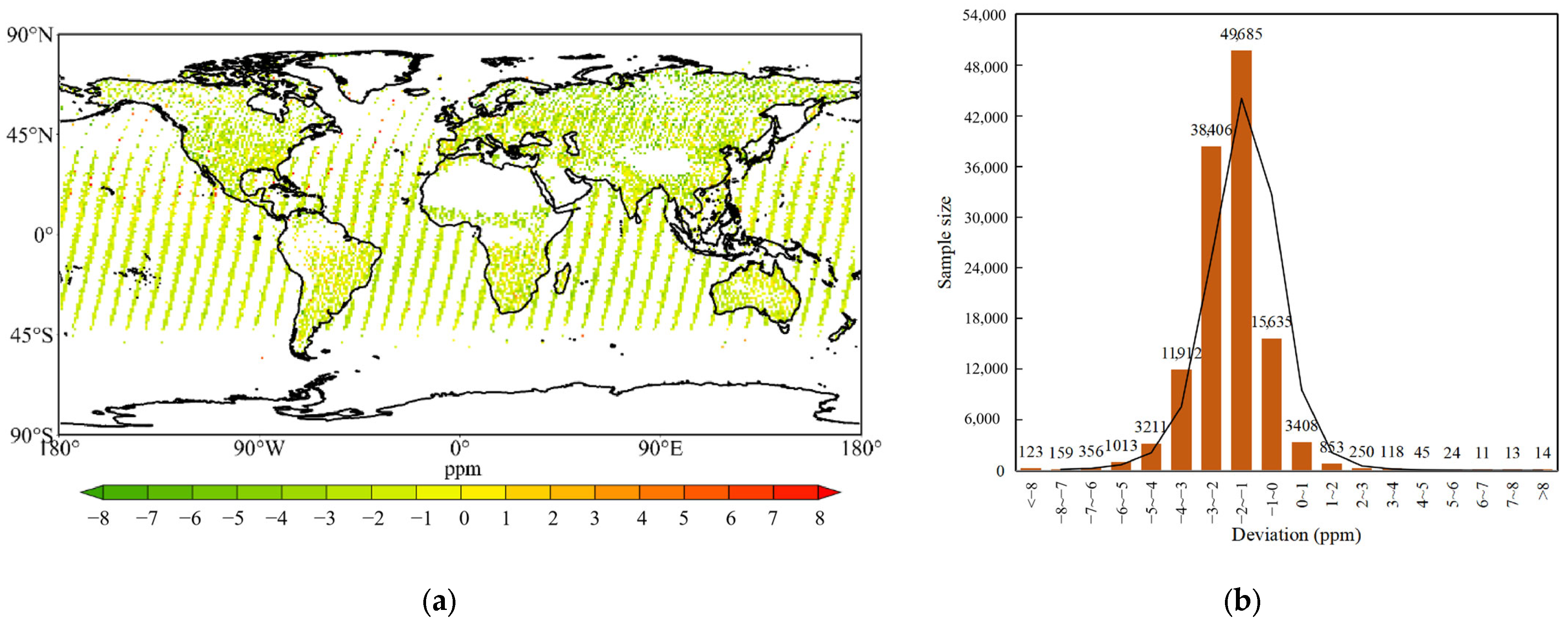
3.1.1. Verification Results of Satellite Observations

Using the column concentration conversion method outlined in Section 2.3.1, the simulated global stratified CO₂ concentrations were first converted into global column concentrations (XCO₂). These simulated XCO₂ values were then interpolated to the locations corresponding to the GOSAT observation points. The deviation between the simulated and GOSAT-observed XCO₂ is calculated by subtracting the GOSAT XCO₂ from the simulated XCO₂. The GOSAT satellite’s effective observation samples cover nearly all continental regions of the world and oceanic areas between 45°S and 45°N, providing wide spatial coverage and making the dataset globally representative (Figure 1). In total, more than 86% of the sample deviations are below 3 ppm. Among these, 30.7% are between −3 and −2 ppm, 39.7% are between −2 and −1 ppm, and 12.5% are between −1 and 0 ppm.

Table 3. Comparison of simulated XCO₂ and GOSAT XCO₂ on a monthly basis.

Time	Sample Size	Simulated Mean (ppm)	Observed Mean (ppm)	Simulated Standard Deviation (ppm)	Observed Standard Deviation (ppm)	RMSE (ppm)	Correlation Coefficient
Jan	6407	385.48	387.24	1.36	1.84	2.15	0.74
Feb	5456	386.03	387.63	1.59	1.92	1.98	0.80
Mar	8285	386.86	388.27	1.88	2.11	1.78	0.86
Apr	8583	387.83	389.27	2.00	2.34	1.81	0.89
May	9396	387.88	389.52	1.74	2.39	2.07	0.86
Jun	10,609	386.94	388.90	1.32	1.74	2.39	0.62
Jul	11,704	385.47	387.57	2.04	2.07	2.48	0.80
Aug	14,258	385.30	387.36	1.64	1.84	2.34	0.81
Sep	14,166	385.44	387.51	1.16	1.33	2.33	0.64
Oct	14,369	385.97	388.10	0.58	1.14	2.36	0.44
Nov	13,207	386.30	388.39	0.42	1.03	2.32	0.28
Dec	8796	386.70	388.78	0.91	1.40	2.35	0.64
Yr	125,236	386.26	388.18	1.67	1.89	2.25	0.79

presents the total number of samples, mean values of simulated XCO₂ and GOSAT XCO₂, standard deviations (SDs), root mean square errors (RMSEs), and correlation coefficients (r) for each month, providing a comparison of the simulated and observed XCO₂ on a monthly scale. A total of 125,236 observed samples were collected throughout the year. The standard deviations of both simulated and observed XCO₂ exhibited similar trends over the course of the year, and the RMSE for both was below 2.48 ppm. The correlation coefficient for most months exceeded 0.62, with an overall annual correlation coefficient reaching 0.79. In general, the simulated XCO₂ concentrations were 0 to 2.00 ppm lower than the GOSAT XCO₂ concentrations. However, both datasets showed high consistency in terms of spatial and temporal distribution, indicating that the GEOS-Chem simulation results in this study accurately reflect the satellite observation data.

3.1.2. Verification Results of Surface Observation

Surface CO₂ concentrations, simulated using the methodology outlined in Section 2.3.2, were validated against observational data from 30 NOAA-ESRL monitoring stations. The correlation coefficients between the simulated and observed surface CO₂ concentrations at all sites are shown in Supplementary Materials Figure S1. At more than 90% of the sites, the correlation coefficient exceeded 0.85, and at over half of the sites, it exceeded 0.95. As shown in Figure 2, CO₂ concentrations at all stations exhibited a general upward trend over the years and displayed different seasonal variations with respect to latitude. Specifically, the observed surface CO₂ concentration in the high latitudes of the Northern Hemisphere, particularly in Europe, showed significant seasonal variation. For example, the annual fluctuation in observed surface CO₂ concentrations at sites such as PAL, HUN, BAL, BSC, BRW, ALT, UUN, and MHD reached about 20 ppm. In contrast, surface CO₂ concentrations in the Southern Hemisphere exhibited smaller fluctuations throughout the year. For example, at sites like USH, BKT, PSA, SEY, ASC, HBA, SYO, and CGO, the annual fluctuation in surface CO₂ concentrations was less than 5 ppm. The simulated surface CO₂ concentrations were highly consistent with those observed at about 80% of the sites, with the mean deviation being less than 2.5 ppm. Overall, the surface CO₂ concentrations simulated by GEOS-Chem in this study align well with the observations from NOAA-ESRL, indicating that the simulation results accurately reflect the spatial and temporal distribution of CO₂ concentrations in the real atmosphere.

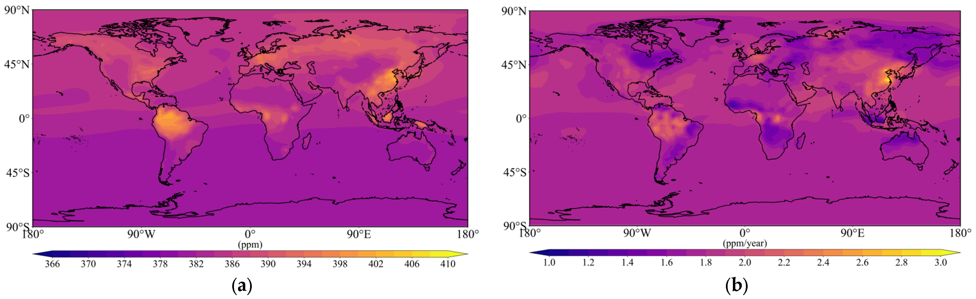
3.2. Temporal and Spatial Characteristics of Global Simulated Atmospheric CO₂ Concentration

The annual average surface CO₂ concentration simulated by GEOS-Chem from 2006 to 2010, as shown in Figure 3a, reveals a global average of 383.7 ppm. The data indicate that CO₂ concentrations over land are consistently higher than over the oceans, and concentrations in the Northern Hemisphere exceed those in the Southern Hemisphere. Specifically, CO₂ concentrations in most of the Northern Hemisphere are above 384 ppm, while in the Southern Hemisphere, particularly south of 20 °S, CO₂ concentrations generally remain below 382 ppm. These regional variations are primarily influenced by natural factors such as the ocean and terrestrial biosphere, which act as carbon sinks, absorbing some of the CO₂ and thereby lowering atmospheric concentrations. The study finds that CO₂ concentrations are particularly high in industrialized and densely populated regions such as eastern China, Southeast Asia, northern Eurasia, Europe, and eastern North America, where the average annual CO₂ concentration ranges from 394 to 406 ppm. These findings are consistent with those reported by Miller et al. (2019) [38] and Hamble et al. (2021) [38], who observed that industrialization and high energy consumption lead to elevated CO₂ levels in these areas. Miller et al. (2019) [38] highlighted the role of energy consumption and air pollution in driving high CO₂ concentrations in industrialized regions, a trend consistent with the current results.

In contrast, CO₂ concentrations in the Southern Hemisphere are generally lower; however, elevated CO₂ levels are observed in northern South America and Central Africa. Specifically, in northern South America, the average annual CO₂ concentration exceeds 398 ppm, and in parts of Central Africa, concentrations can reach over 396 ppm. These findings are in line with Xie et al. (2024) [39], who demonstrated that deforestation, natural gas extraction, and fossil fuel activities are significant contributors to the rise in CO₂ concentrations in these regions. Therefore, while there are notable regional differences in global CO₂ concentrations, these variations are not only driven by natural factors but also by anthropogenic activities such as industrialization, deforestation, and fossil fuel extraction, which is consistent with findings from various studies.

As shown in Figure 3b, the average annual growth rate of surface CO₂ concentration simulated by GEOS-Chem from 2006 to 2010 is 1.8 ppm year⁻¹. There are significant regional variations in the CO₂ growth rates. Eastern China exhibits the fastest annual increase in CO₂ concentration, with the maximum rate reaching up to 3.0 ppm year⁻¹. This rapid growth is primarily driven by the high population density and intense industrial energy consumption in Eastern China, where industrial emissions are the principal contributor to the accelerated rise in atmospheric CO₂ levels. These findings align with the study by Liu et al. (2024) [11], which underscores the substantial emissions from industrial activities, particularly in densely populated urbanized regions of eastern China. In addition to Eastern China, regions such as southeastern North America, northern South America, Europe, and Central Africa show annual CO₂ growth rates ranging from 1.8 to 2.4 ppm year⁻¹. These regions also experience elevated industrial emissions, further corroborating the observed higher CO₂ growth rates. In contrast, Southeast Asia exhibits a markedly lower growth rate (1.5 ppm year⁻¹), reflecting reduced industrial emissions and energy demand compared to high-emission regions. This disparity can be attributed to lower industrial emissions and less intensive energy consumption in Southeast Asia. Research by Liu et al. (2023) [40] suggests that despite rapid industrialization, Southeast Asia still exhibits lower per capita CO₂ emissions compared to regions such as China and North America, leading to a relatively lower growth rate in atmospheric CO₂ concentration.

The global distribution of CO₂ concentrations exhibits typical seasonal variation characteristics (Figure 4). Winter is the season with the highest CO₂ concentration of the year, with a global average simulated CO₂ concentration of 385.4 ppm. In regions such as much of Europe, northern Eurasia, and southeastern China, CO₂ concentrations exceed 400 ppm, and in parts of central Europe, central Asia, and eastern China, concentrations even surpass 410 ppm. Summer, on the other hand, is the season with the lowest CO₂ concentration, with a global average simulated CO₂ concentration of 381.5 ppm. During this period, CO₂ concentrations are highest near the equator, ranging from 380 to 400 ppm. North of 45°N, CO₂ concentrations are generally below 380 ppm, and in some areas of central Europe, concentrations can even drop below 370 ppm. The CO₂ concentration in spring and autumn lies between that of winter and summer, with the high-concentration regions showing a distribution similar to that of winter. These seasonal variations can be attributed to changes in temperature and biological activity. In winter, due to lower temperatures and increased heating demands, as well as higher energy consumption in industrialized regions, CO₂ concentrations rise, especially in regions such as eastern China and Europe. In contrast, during the summer, increased photosynthesis by plants leads to significant CO₂ absorption, resulting in lower concentrations, particularly in the higher latitudes of the Northern Hemisphere where vegetation growth and temperature conditions have a suppressive effect on CO₂ levels [41]. Moreover, the CO₂ concentrations in spring and autumn are intermediate, influenced by the combined effects of temperature, plant activity, and climatic conditions [42]. In spring, warming temperatures and the start of plant growth cause a slight reduction in CO₂ concentrations, while autumn sees an uptick due to the decay of plant matter and cooler temperatures [9]. Therefore, seasonal fluctuations are not only a natural consequence of climate changes but also the result of the interplay between biological and human activities, especially in industrialized and energy-intensive areas where CO₂ concentrations fluctuate more significantly.

Figure S2 shows the global average surface CO₂ concentration for each month from 2006 to 2010 as simulated by GEOS-Chem. The global average CO₂ concentration has increased rapidly year by year, and the atmospheric CO₂ concentration has increased by about 7.0 ppm in 5 years. The regression line was obtained by the linear fitting of monthly CO₂ concentrations, and it can be inferred that the CO₂ concentration increased by about 0.13 ppm per month and the coefficient of determination reached more than 0.42. In addition, it can be seen from the figure that the global atmospheric average CO₂ concentration has significant seasonal fluctuations.

Figure S3 shows the monthly average global surface CO₂ concentration and growth rate, which is used to further explore the month-to-month variation in global CO₂ concentration. As can be seen from the figure, the global average CO₂ concentration has an obvious seasonal fluctuation cycle, and the global average CO₂ concentration gradually increases from January to March, reaching the annual peak value (389.3 ppm), and then gradually decreases, reaching the annual trough value (383.1 ppm) in August, and the difference in CO₂ concentration in each month of the year is up to 6.2 ppm. This seasonal fluctuation is consistent with previous studies, which have also shown that CO₂ concentration peaks in winter and reaches its lowest point in summer due to the combined effects of biological and physical processes, such as increased photosynthesis in summer and higher fossil fuel consumption in winter, as reported by Keeling et al. (2005) [43]. In contrast, the month-to-month trend of the growth rate of global mean CO₂ concentration shows an inverse phase change compared with CO₂ concentration. The growth rate of CO₂ concentration in September was the highest (1.95 ppm year⁻¹), the growth rate of CO₂ concentration in February was the lowest (1.62 ppm year⁻¹), and the difference in monthly CO₂ concentration growth rate throughout the year was the highest at 0.33 ppm year⁻¹. Similar to these findings, other studies have also reported that the CO₂ growth rate is inversely related to the concentration, with a higher growth rate observed during winter months, especially due to heating demands and increased fossil fuel consumption.

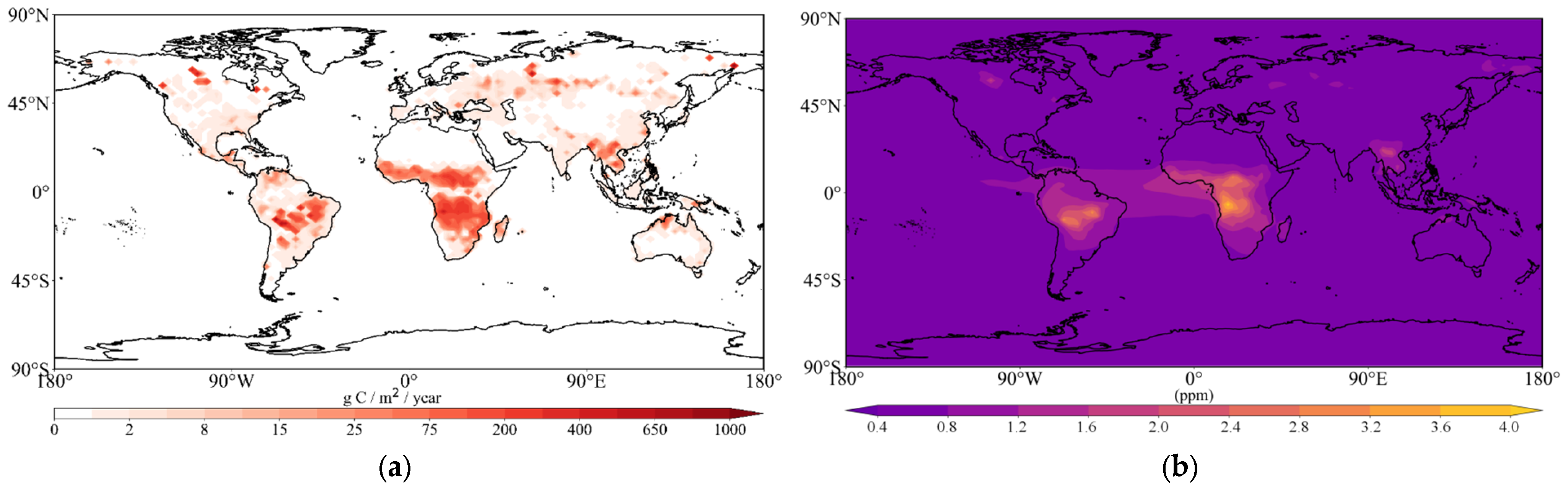
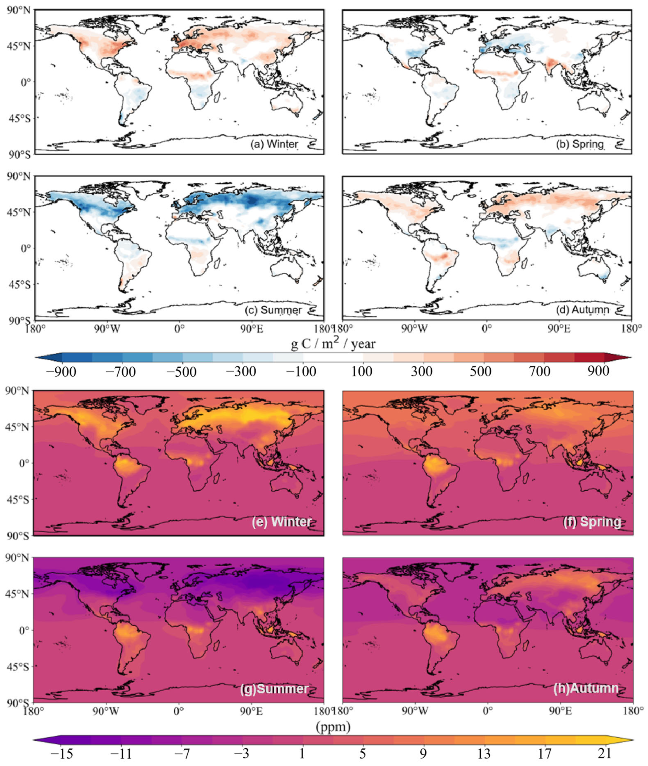
3.3. Effects of Different CO₂ Sources on Atmospheric CO₂ Concentration

Figure 5 and Table S2 show the global fluxes of eight different types of CO₂ source–sinks simulated by GEOS-Chem in this study. Among them, fossil fuel emissions mainly include CO₂ emissions from natural gas, coal, oil, and other fossil fuels. Biomass combustion emissions are mainly CO₂ emissions from forest fires, grassland fires, crop straw burning, household firewood burning, domestic waste burning, and so on. Equilibrium biosphere refers to the net ecosystem productivity calculated by the sum of total primary productivity and respiration without considering anthropogenic influence, with seasonal cyclical changes, but the annual net total is 0. Nautical emissions are the emissions caused by marine navigation activities. Aviation emissions include CO₂ emissions from aviation activities at every layer of the atmosphere. Ocean exchange refers to the amount of CO₂ exchanged between the ocean and the atmosphere. Chemical sources mainly include the oxidation of carbon monoxide, methane, and other species into CO₂ in the atmosphere. According to the simulation results, fossil fuel combustion is the world’s largest source of CO₂ emissions, emitting 8.81 Gt C year⁻¹ into the atmosphere. Biomass combustion is the second largest source of CO₂ emissions globally, emitting 2.00 Gt C year⁻¹ into the atmosphere, accounting for about a quarter of fossil fuel emissions. Aviation and navigation emit less than 0.3 Gt C of CO₂ into the atmosphere throughout the year, but as an important source of CO₂ in the atmosphere, their role cannot be ignored. The land and ocean are the most important CO₂ sinks in the world and maintain the dynamic balance of CO₂ in the atmosphere by absorbing CO₂. The land and ocean are the most important CO₂ sinks in the world and maintain the dynamic balance of CO₂ in the atmosphere by absorbing CO₂.

In the process of industrialization and urbanization, global CO₂ emissions from fossil fuels have been increasing over the past few decades. The regional distribution of fossil fuel emissions is uneven, with the largest emitters globally being China, the United States, and India, but some small countries and regions have high per capita emissions. In addition, there are differences in the energy structure of fossil fuels, such as some countries’ energy mainly being from fossil fuels such as coal, while others rely on natural gas, nuclear energy, and other energy sources. The burning of fossil fuels releases large amounts of CO₂, far more than other sources of emissions. This uneven distribution is consistent with the findings of Liu et al. (2020), which show that, despite lower total emissions in some developing countries, their per capita emissions are higher than the global average, especially in countries that are heavily dependent on high-carbon sources such as Saudi Arabia and Argentina [44]. Global CO₂ emissions from fossil fuels are one of the main causes of climate change, and the CO₂ produced can persist in the atmosphere for decades or even longer, causing global warming and climate crises and becoming a global problem [45].

As can be seen from the global distribution of fossil fuel emissions in Figure 6a, the high-value area of fossil fuel emissions is mainly distributed in the Northern Hemisphere, especially in the United States, Europe, India, China, and other regions, and the local annual CO₂ emissions can even exceed 2500 g C/m². There are also pockets of high fossil fuel emissions along the southeastern coast of South America, Africa, and Australia. The spatial distribution of fossil fuel emissions depends on many factors, including geographic location, the level of economic development, energy use patterns, industrial structure, population density, and more. According to Rayner et al. (2010), industrialized nations exhibit dense clusters of energy-intensive infrastructure (e.g., power plants, refineries), where rapid economic growth correlates with elevated carbon emissions [46]. The spatial distribution characteristics of surface atmospheric CO₂ concentration affected by fossil fuel emissions (Figure 6b) are very similar to the spatial distribution characteristics of fossil fuel emissions themselves. The increase in CO₂ concentration caused by fossil fuel emissions is more pronounced in the Northern Hemisphere than in the Southern Hemisphere, which is in accordance with the more intensive population, economic, and industrial development in the Northern Hemisphere. Increases in CO₂ concentrations are particularly significant in eastern North America, Europe, and eastern Asia. The added value of CO₂ concentration caused by fossil fuel emissions generally exceeds 5 ppm in eastern North America, reaching a maximum of 13 ppm; generally exceeds 7 ppm in Europe, reaching a maximum of about 15 ppm; and generally exceeds 8 ppm in eastern China, reaching a maximum of about 25 ppm.

The Global Carbon Budget 2024 report states that land-use change carbon emissions are the second largest source of CO₂ emissions after fossil fuel combustion, of which biomass combustion is an important component. In some developing countries and regions, biomass combustion dominates all sources of carbon emissions [47]. Unlike fossil fuel emissions, CO₂ emitted from biomass combustion is not a new carbon source but comes from atmospheric CO₂ previously absorbed by plants, so biomass energy is also considered a renewable energy source [48]. Biomass combustion has strong spatial and temporal heterogeneity, showing randomness, periodicity, wide range, multi-point sources, difficult monitoring, and other characteristics, and has a very important contribution to the spatial and temporal distribution and dynamic changes in global CO₂. Biomass burning will have an impact on the climate in the short term, but the impact on the climate in the long term is dynamically balanced. However, the problems brought about by land-use change, water resource consumption, and deforestation still need people’s attention.

As can be seen from Figure 7a, carbon emissions from biomass combustion are widely distributed globally, particularly in key regions such as Africa, South America, and the Southeast Asian Peninsula, where these emissions significantly impact atmospheric CO₂ concentrations. In Africa, biomass burning activities are primarily concentrated in central and southern regions, with annual CO₂ emissions generally exceeding 15 g C/m², and in some areas surpassing 400 g C/m², 30–45% higher than Global Fire Emissions Database (GFEDv4) estimates (1° × 1° resolution). This discrepancy arises from our model’s 2.5° × 2.0° grid resolving small-scale fires (<50 km) omitted in coarser inventories. Such extreme emissions result in near-surface CO₂ increases exceeding 4.0 ppm throughout the year, a magnitude comparable to Amazon Basin fires but with distinct seasonal drivers: African enhancements persist 8–10 months due to frequent agricultural burning facilitated by prolonged dry seasons, as reported by Archibald et al. (2022) [49], whereas Amazonian peaks last 3–4 months and are amplified by El Niño-induced droughts [50]. These findings demonstrate that biomass burning in both regions leads to similar annual CO₂ increases (~4 ppm) yet highlight a critical limitation of uniform parameterizations in emission inventories (e.g., GFEDv4), which underestimate CO₂ persistence in regions dominated by small fires.

Moreover, this study finds that biomass combustion in central and eastern South America and the Southeast Asian Peninsula also significantly influences local atmospheric CO₂ levels (Figure 7b), with annual CO₂ emissions typically above 25 g C/m², resulting in CO₂ concentration increases exceeding 1.2 ppm. This is consistent with the findings of Field et al. (2009), who reported that biomass burning in Southeast Asia, particularly in Indonesia, has been associated with CO₂ concentration increases ranging from 1.5 to 2.0 ppm [51]. Similarly, Andreae and Merlet (2001) provided comparable data, indicating that during fire seasons, CO₂ concentration increases in Africa and South America could reach 3–4 ppm, further validating the observations made in this study [52].

By comparing these results with existing research, it is evident that the data from this study are broadly consistent with previous findings, reinforcing the significant impact of biomass combustion on global CO₂ concentrations, especially in critical regions like Africa, South America, and Southeast Asia. These findings are crucial for understanding the global carbon cycle and its implications for climate change.

Influenced by climate change, soil moisture, vegetation growth, soil temperature, and land use patterns, CO₂ flux between vegetation and the ecosystem has obvious seasonal fluctuations [53]. The equilibrium biosphere exchange flux in the GEOS-Chem model refers to the net difference between the total amount of CO₂ absorbed by plants through photosynthesis and the total amount of ecosystem respiration, which has seasonal characteristics, but the total annual flux remains 0. Specifically, summer is usually the strongest season for CO₂ absorption, because vegetation growth and photosynthesis are enhanced in summer, which increases the absorption of CO₂ from the atmosphere. The strongest release of CO₂ from plants occurs in winter, when vegetation growth slows and soil respiration increases, leading to an increase in CO₂ release into the atmosphere. Based on this feature, this study analyzed the equilibrium biosphere exchange flux and its impact on atmospheric CO₂ concentration on a seasonal scale.

Figure 8a–d show the equilibrium biosphere exchange carbon flux for the four seasons. Positive values generally represent net CO₂ fluxes from ecosystems to the atmosphere (terrestrial carbon sources), and negative values represent net CO₂ removals from ecosystems (terrestrial carbon sinks). These fluxes exhibit strong spatial–seasonal coherence with vegetation density. In winter, the equilibrium biosphere exchange flux is dominated by terrestrial carbon sources in the equatorial regions of South America and Africa, North America, Eurasia except India, and Australia and peaks in Europe at more than 600 g C/m². This aligns with observations of reduced photosynthesis under cold stress, where ecosystem respiration exceeds carbon uptake during winter months, as found by Reichstein et al. (2013) [54]. South of the equator, South America, Africa, and India are dominated by terrestrial carbon sinks, and the overall carbon sinks are weak. This is likely due to the reduced vegetation activity during the colder months, leading to lower carbon sequestration. Summer reverses this pattern: carbon sinks dominate equatorial and northern regions. Northern Central Asia shows the strongest sink (>900 g C/m²), aligning with satellite-observed greening trends [55], while North America’s sink exceeds 500 g C/m². Spring and autumn fluxes are transitional, with magnitudes 50–70% lower than winter/summer, reflecting balanced photosynthesis–respiration dynamics [56]. It is worth noting that the terrestrial carbon source effect in India is the strongest in the spring, and the whole region is basically more than 300 g C/m², driven by pre-monsoon crop burning [57]. The changes in surface atmospheric CO₂ concentration caused by the equilibrium biosphere exchange flux (Figure 8e–h) also have seasonal fluctuations, which align with the findings from Kondo et al., who noted that seasonal changes in terrestrial CO₂ fluxes lead to significant CO₂ concentration variations, particularly in tropical and temperate regions. The equilibrium biosphere exchange flux causes a significant increase in atmospheric CO₂ concentration in winter, especially in northern and eastern North America, equatorial South America, Africa and Indonesia, northern Eurasia, the Southeast Asian Peninsula, and central and eastern China. CO₂ concentrations in Eurasia generally increase by more than 9 ppm. In summer, the balanced biosphere flux results in a reduction in CO₂ concentrations of more than 7 ppm in continental regions north of 45°N latitude. It is worth noting that the equatorial regions of South America, Africa, and Indonesia show a consistent increase in CO₂ concentrations throughout the year, driven by vigorous vegetation growth in tropical regions, such as tropical rainforests and savannas.

The net land exchange flux is used to represent the net annual budget or residual amount of CO₂ from the terrestrial biosphere. In GEOS-Chem, this partial CO₂ flux is set to a fixed value and divided according to different regions. A total of 11 subregions have been identified on a global scale, and the net land exchange flux within each subregion is nearly consistent. According to Figure 9a, Northern North America and South America are the two most typical net terrestrial exchange carbon sources in the world, while other regions are net terrestrial exchange carbon sinks, and the top three regions are Southern Africa, Europe, and Southern South America. The global net land exchange flux was −5.28 Gt C, dominated by carbon sinks throughout the year. Correspondingly, the surface atmospheric CO₂ concentration affected by the net land exchange flux (Figure 9b) showed similar distribution characteristics, and the overall performance of the whole year was to reduce the atmospheric CO₂ concentration. In northern South America, the change in atmospheric CO₂ concentration due to net land exchange flux was less than 0.8 ppm, and in Europe, the change in atmospheric CO₂ concentration due to net land exchange flux was more than 4.4 ppm.

Navigation is one of the important sources of greenhouse gas emissions from human activities. According to the third study of greenhouse gas emissions published by the International Maritime Organization (IMO), CO₂ emissions from shipping account for about 2.2% of the total global CO₂ emissions. In 2018, the total CO₂ emissions of the global shipping industry were 1.01 billion tons, of which the CO₂ emissions of maritime transport were 960 million tons, accounting for more than 95%, occupying a dominant position in shipping. CO₂ emissions from land transport and port activities are smaller, at 0.4 million tonnes and 0.1 million tonnes, respectively. In addition, CO₂ emissions from the shipping industry continue to grow, with global CO₂ emissions from shipping increasing by 28.9% between 2007 and 2018, with the number of ships increasing by more than 50%. At the same time, the improvement in ship transportation efficiency and fuel utilization rate can only partially offset the increase in emissions caused by the increase in the number of ships [58,59]. Notably, this 28.9% growth rate exceeds the 22% global maritime CO₂ increase reported by Jalkanen et al. (2008) for 2000–2008 [60], suggesting a potential regional acceleration in emission hotspots like Europe despite global efficiency policies.

Figure 10a shows the spatial distribution of global maritime carbon emissions in 2010. The high-value areas of marine carbon emissions are closely consistent with marine activities, and the coastal areas and common routes are usually the areas with high CO₂ emissions. This is because these areas usually have a large number of ports and transportation, which require a large amount of fuel consumption. Maritime CO₂ emissions from European coastal areas are among the highest in the world, exceeding 500 g C/m² in some areas. This is because the European region has many ports and shipping centers, its maritime transport business is large, and the corresponding carbon emissions are relatively high. Secondly, the economic activity of Europe’s coastal regions is intensive, including several industries such as manufacturing, trade, and tourism, which require a large amount of support from shipping services, further increasing shipping carbon emissions. In addition, the European coastal region has a large maritime fleet, and these vessels often use traditional oil power systems and have relatively high carbon emissions. The spatial distribution of global atmospheric CO₂ concentration increase caused by navigation (Figure 10b) is highly consistent with marine CO₂ emissions, in which the increase in CO₂ concentration in the Northern Hemisphere is significantly higher than that in the Southern Hemisphere, and it is mainly distributed across the two sides of the Atlantic and Pacific oceans. Coastal areas in northern Germany and Denmark have the highest CO₂ increases in the world, with local CO₂ increases from marine CO₂ emissions reaching up to 0.48 ppm or more. This observed 0.48 ppm peak contrasts with the 0.32–0.41 ppm range predicted by Viana et al. (2014) for North Atlantic shipping corridors [61], a discrepancy potentially attributable to two factors omitted in current models: (1) the non-linear enhancement of emissions from port-side vessel activities, such as auxiliary engine use during docking, and (2) the prolonged near-coastal atmospheric residence time due to frequent low-speed navigation in congested waterways, which exacerbates local CO₂ accumulation.

Aviation activities are a significant source of global greenhouse gas emissions. The bulk of aviation’s carbon emissions come from CO₂ produced by burning fuel in jet engines. According to the International Civil Aviation Organization (ICAO), CO₂ emissions from aviation account for about 2–3% of total global CO₂ emissions. Carbon emissions from aviation have grown over the past few decades and are expected to continue to increase in the future. The International Energy Agency (IEA), based on future economic growth and expansion of the aviation industry, as well as technology and policy measures for the aviation industry in the future, predicts that global carbon emissions from the aviation industry could grow 2–3 times by 2040. However, this projection contrasts with the 1.7-fold growth estimated by Graver et al. (2020), which assumes a 50% sustainable aviation fuel adoption by 2040. This highlights the critical role of fuel policy acceleration in emission mitigation, as discussed in the ICCT Report (2020) [62]. The IEA 2023 report, “The Future of Petrochemicals: Towards more sustainable plastics and fertilisers”, also discusses the long-term outlook. Aviation carbon emissions vary based on flight length. Long-haul international flights contribute significantly more to carbon emissions because they use more fuel, while short-haul flights typically have lower emissions. In addition, the impact of CO₂ emitted at high altitudes on climate change is more significant than that of CO₂ emitted at ground level. This is because aviation carbon emissions, occurring mainly at high altitudes, are more easily dispersed around the world, and their greenhouse effect is more intense at higher elevations. For example, the Fifth Assessment report released by the United Nations Intergovernmental Panel on Climate Change (IPCC) pointed out that the contribution of carbon emissions from aviation activities to global warming is about 3.5–4.9%. However, this estimate primarily accounts for the direct CO₂ impact and does not fully capture the broader effects. Recent studies by Brasseur et al. (2016) show that when including non-CO₂ effects, such as contrail cirrus, aviation’s total radiative forcing could account for 7.3% of anthropogenic forcing in 2011 [63], suggesting that conventional attribution methods may underestimate the full climate impact of aviation.

Affected by many factors such as flight route, flight speed, aircraft type, and meteorological conditions, the height of aviation carbon emissions is not fixed. Figure 11a shows the aggregate CO₂ emissions from aviation at each vertical level of the atmosphere. Aviation CO₂ emissions exhibit a strong spatial correlation with major international airports, highlighting key emission hotspots in global air transport networks. Among them, the United States, Europe, southeast China, and Japan are the regions with the highest emissions from global aviation, with emissions reaching more than 20 g C/m². In addition, the distribution of aviation emissions is closely related to the route, and this part comes from the CO₂ emitted by the aircraft during flight. Unlike other sources of emissions, aviation CO₂ emissions occur at both surface and high altitudes and at different altitudes in different parts of the world. Therefore, this study explores the impact of aviation emissions on the average atmospheric CO₂ concentration at each layer. As can be seen from Figure 11b, the increase in the mean atmospheric CO₂ concentration of each layer caused by aviation CO₂ emissions is higher in the Northern Hemisphere and lower in the Southern Hemisphere. Due to the enhanced mixing in the upper atmosphere, the distribution of CO₂ concentration is zonally uniform across the globe, with a north–south gradient of about 0.04 ppm. At the same time, this study also explored the changes in surface atmospheric CO₂ concentration affected by aviation CO₂ emissions in 2010 (Figure S4). The increase in surface CO₂ concentration was also high in the Northern Hemisphere and low in the Southern Hemisphere, but it was prominent in the continental region. Among them, the United States and Europe are the two major regions where the surface atmospheric CO₂ concentration increased significantly due to aviation CO₂ emissions. The local CO₂ concentration increase value can reach more than 0.1 ppm, and it is one-to-one corresponding to the airport location.

CO₂ exchange between the ocean and atmosphere is one of the important processes affecting the global carbon cycle and one of the important factors affecting global climate change. Overall, the ocean, as a major global carbon sink, absorbs about 25% of CO₂ emissions from the atmosphere, though recent studies suggest this proportion may decrease by 5–10% per decade due to tropical source intensification [64]. In tropical areas, the temperature of the sea surface is higher, and these areas usually have a greater amount of sunlight. The observed CO₂ emissions in the tropical eastern Pacific exceed IPCC AR6 model estimates by 12–15% [65], likely associated with enhanced upwelling under climate variability. In polar sea regions, sea surface temperatures are cooler, and the oceans in these regions typically absorb CO₂ with the Norwegian Sea sink showing 20% higher efficiency than pre-2000s levels, possibly linked to sea ice retreat effects [18]. The rate at which the ocean absorbs CO₂ from the atmosphere varies with the seasons, with a faster rate in winter and a slower rate in summer. This seasonal contrast (3:1 winter–summer ratio in absorption rates) aligns with biological pump enhancements observed in Arctic winter phytoplankton blooms. The surface of the ocean is the main area of CO₂ absorption and release, and the deep ocean usually has relatively high CO₂ concentrations. Ocean circulation also has an important effect on the exchange of CO₂, particularly the circumantarctic CO₂ source, which shows interannual variability 30% greater than Coupled Model Intercomparison Project Phase 5 model projections [66]. Figure 12 provides quantitative validation and spatial refinement of the ocean–atmosphere CO₂ exchange dynamics described above. Positive values indicate that CO₂ enters the atmosphere from the ocean—that is, the ocean emits CO₂ (marine CO₂ source)—while negative values represent the passage of CO₂ from the atmosphere into the ocean, i.e., the uptake of CO₂ by the ocean (ocean CO₂ sink). As can be seen from Figure 12a, the tropical region and the circumantarctic region are the main sources of ocean CO₂ exchange in the world, among which the tropical eastern Pacific region and the junction of the Arabian Sea and the Gulf of Aden are the regions with the strongest annual marine CO₂ emissions, with a local maximum of more than 36 g C/m². The Norwegian Sea and Labrador Bay near the Arctic Circle are the two regions with the strongest annual marine CO₂ absorption, with local CO₂ absorption fluxes reaching above 54 g C/m². As can be seen from Figure 12b, the impact of ocean exchange on the surface atmospheric CO₂ concentration is mainly manifested as the reduction in global CO₂ concentration. Specifically, changes in CO₂ concentrations at the ocean surface decrease from the equator to the poles. The annual ocean exchange flux decreased the CO₂ concentration in equatorial waters by 0~0.8 ppm. The CO₂ concentration in the sea area near 45°S latitude decreased by 1.1~1.5 ppm; The CO₂ concentration in the North Atlantic Ocean to the south of the Arctic Ocean decreased by more than 1.2 ppm, of which the highest CO₂ concentration in the east and south of Greenland exceeded 1.6 ppm.

The incorporation of CO₂ generated by the oxidation of non-combustion carbon species, as demonstrated by Nassar et al. (2010) in the modified GEOS-Chem model, addresses a critical gap in traditional atmospheric CO₂ inventories [12].

This refinement aligns with studies demonstrating that unaccounted-for oxidative CO₂ sources (e.g., smoldering biomass residues, carbonate weathering) introduce regional simulation biases of 0.5–1.5 ppm, particularly in fire-prone ecosystems. The results corroborate this spatial dependency, revealing that regions with intense biomass burning (e.g., Central Africa and Southeast Asia) exhibit the largest corrections (ΔCO₂ > 1.0 ppm annually), while temperate zones (e.g., Europe, eastern North America) show moderate adjustments (~0.25 ppm) (Figure 13). These disparities reflect the heterogeneous distribution of oxidative processes and underscore the need for region-specific emission inventories in climate models. The spatial trends in chemical source fluxes (Figure 13b) mirror global patterns of land-use change and biomass combustion reported in the GFEDv4. For instance, the >10 g C/m² flux over South Asia and Central Africa corresponds to GFEDv4’s “burned area” hotspots, where forest harvesting and agricultural fires dominate oxidative CO₂ production. This consistency with independent datasets strengthens the validity of the model’s spatial adjustments. However, discrepancies in northern Africa—where simulated fluxes exceed GFEDv4’s fire-driven estimates—suggest additional contributions from carbonate weathering or undocumented land-use changes, a hypothesis supported by Kok et al. (2021) in their analysis of Saharan dust–CO₂ interactions [67].

Temporally, the persistent > 1.0 ppm corrections in Central Africa and eastern China (Figure 13a) highlight the compounding effects of biomass burning and industrial emissions. These regions exemplify the intersection of natural and anthropogenic oxidative processes, a dynamic poorly resolved in earlier models like Carbon Tracker. The results contrast with the spatially uniform CO₂ sink assumptions (<0.5 ppm) for tropical reforestation proposed by Bastin et al. (2019) [68], suggesting that current climate policies neglecting oxidative CO₂ sources may overstate the efficacy of reforestation in offsetting combustion emissions. National policies should prioritize integrating oxidative CO₂ sources (e.g., biomass smoldering, rock weathering) into emission inventories and implementing region-specific controls, such as seasonal fire bans and geochemical interventions, to mitigate these non-combustion fluxes. These targeted measures enhance climate model accuracy while complementing existing emission reduction frameworks.

4. Conclusions

The study identifies fossil fuel combustion as the dominant source of atmospheric CO₂ emissions, contributing 8.81 Gt C/year, while biomass combustion ranks second, producing approximately 2.00 Gt C/year—about a quarter of fossil fuel emissions in 2010. Other significant contributors include aviation and maritime activities, as well as chemical oxidation processes.

The influence of different CO₂ sources on atmospheric concentrations is strongly correlated with their spatial distribution and emission magnitudes. Fossil fuel combustion emissions are predominantly concentrated in the Northern Hemisphere, particularly in the eastern United States, Europe, East Asia, and India, with eastern China exhibiting the highest regional contribution. Biomass combustion emissions are more widespread, with Africa being the largest source. Regions such as South America, Africa, and Southeast Asia experience the most pronounced CO₂ concentration increases due to biomass combustion. Aviation and maritime activities contribute significantly to global CO₂ emissions, with emissions concentrated along major flight corridors, airports, shipping lanes, and ports. Similarly, chemical oxidation processes contribute to CO₂ formation, particularly in China and Central Africa, although their impact is mainly observed in model simulations rather than directly increasing measured atmospheric CO₂ concentrations.

The ocean and terrestrial biosphere act as a major CO₂ sink, offsetting a substantial fraction of emissions. The ocean absorbs approximately 2.22 Gt C/year, with the strongest uptake occurring in the Norwegian Sea and Labrador Bay, while the terrestrial biosphere has a net uptake of 5.28 Gt C/year. The distribution of terrestrial CO₂ fluxes varies globally, with North America and northern South America acting as net carbon sources, whereas most other regions function as carbon sinks. The seasonal dynamics of atmospheric CO₂ are largely influenced by terrestrial biosphere activity. During summer, increased photosynthesis reduces atmospheric CO₂ concentrations in the Northern Hemisphere while contributing to localized increases in the Southern Hemisphere, creating a distinct seasonal cycle that affects global CO₂ distribution patterns.

The interplay between CO₂ sources and sinks drives atmospheric CO₂ variations, influencing global climate dynamics. Understanding these mechanisms is essential for refining climate models and formulating effective mitigation strategies. To improve global carbon management, future research should focus on refining emission inventories, particularly for small-scale sources like biomass burning, and enhancing model representations of biogeochemical processes. Additionally, regional mitigation efforts should be assessed to tailor strategies for high-emission sectors, such as aviation and maritime transport. These improvements are crucial for strengthening the effectiveness of climate policies and ensuring more accurate predictions of CO₂ dynamics.

References

1. Friedlingstein, P.; O’Sullivan, M.; Jones, M.W.; Andrew, R.M.; Hauck, J.; Landschützer, P.; Le Quéré, C.; Li, H.; Luijkx, I.T.; Olsen, A.; et al. Global Carbon Budget 2024. Earth Syst. Sci. Data Discuss. 2024, 1–133. [Google Scholar] [CrossRef]
2. Peylin, P.; Law, R.M.; Gurney, K.R.; Chevallier, F.; Jacobson, A.R.; Maki, T.; Niwa, Y.; Patra, P.K.; Peters, W.; Rayner, P.J.; et al. Global Atmospheric Carbon Budget: Results from an Ensemble of Atmospheric CO2 Inversions. Biogeosciences 2013, 10, 6699–6720. [Google Scholar] [CrossRef]
3. Gaubert, B.; Stephens, B.B.; Basu, S.; Chevallier, F.; Deng, F.; Kort, E.A.; Patra, P.K.; Peters, W.; Rödenbeck, C.; Saeki, T.; et al. Global Atmospheric CO2 Inverse Models Converging on Neutral Tropical Land Exchange but Disagreeing on Fossil Fuel and Atmospheric Growth Rate. Biogeosciences 2019, 16, 117–134. [Google Scholar] [CrossRef] [PubMed]
4. Kukkonen, J.; Olsson, T.; Schultz, D.M.; Baklanov, A.; Klein, T.; Miranda, A.I.; Monteiro, A.; Hirtl, M.; Tarvainen, V.; Boy, M.; et al. A Review of Operational, Regional-Scale, Chemical Weather Forecasting Models in Europe. Atmos. Chem. Phys. 2012, 12, 1–87. [Google Scholar] [CrossRef]
5. Bauska, T.K.; Joos, F.; Mix, A.C.; Roth, R.; Ahn, J.; Brook, E.J. Links between Atmospheric Carbon Dioxide, the Land Carbon Reservoir and Climate over the Past Millennium. Nat. Geosci. 2015, 8, 383–387. [Google Scholar] [CrossRef]
6. Keenan, T.F.; Prentice, I.C.; Canadell, J.G.; Williams, C.A.; Wang, H.; Raupach, M.; Collatz, G.J. Recent Pause in the Growth Rate of Atmospheric CO2 Due to Enhanced Terrestrial Carbon Uptake. Nat. Commun. 2016, 7, 13428. [Google Scholar] [CrossRef]
7. Zeng, N.; Han, P.; Liu, Z.; Liu, D.; Oda, T.; Martin, C.; Liu, Z.; Yao, B.; Sun, W.; Wang, P.; et al. Global to Local Impacts on Atmospheric CO2 from the COVID-19 Lockdown, Biosphere and Weather Variabilities. Environ. Res. Lett. 2022, 17, 015003. [Google Scholar] [CrossRef]
8. Feng, L.; Palmer, P.I.; Yang, Y.; Yantosca, R.M.; Kawa, S.R.; Paris, J.-D.; Matsueda, H.; Machida, T. Evaluating a 3-D Transport Model of Atmospheric CO2; Using Ground-Based, Aircraft, and Space-Borne Data. Atmos. Chem. Phys. 2011, 11, 2789–2803. [Google Scholar] [CrossRef]
9. Jalkanen, J.-P.; Brink, A.; Kalli, J.; Pettersson, H.; Kukkonen, J.; Stipa, T. A Modelling System for the Exhaust Emissions of Marine Traffic and Its Application in the Baltic Sea Area. Atmos. Chem. Phys. 2009, 9, 9209–9223. [Google Scholar] [CrossRef]
10. Suntharalingam, P.; Spivakovsky, C.M.; Logan, J.A.; McElroy, M.B. Estimating the Distribution of Terrestrial CO2 Sources and Sinks from Atmospheric Measurements: Sensitivity to Configuration of the Observation Network. J. Geophys. Res. Atmos. 2003, 108, 1–22. [Google Scholar] [CrossRef]
11. Liu, H.; Zhang, Z.; Cai, X.; Wang, D.; Liu, M. Investigating the Driving Factors of Carbon Emissions in China’s Transportation Industry from a Structural Adjustment Perspective. Atmos. Pollut. Res. 2024, 15, 102224. [Google Scholar] [CrossRef]
12. Nassar, R.; Jones, D.B.A.; Suntharalingam, P.; Chen, J.M.; Andres, R.J.; Wecht, K.J.; Yantosca, R.M.; Kulawik, S.S.; Bowman, K.W.; Worden, J.R.; et al. Modeling Global Atmospheric CO2; with Improved Emission Inventories and CO2; Production from the Oxidation of Other Carbon Species. Geosci. Model Dev. 2010, 3, 689–716. [Google Scholar] [CrossRef]
13. Randerson, J.T.; Thompson, M.V.; Conway, T.J.; Fung, I.Y.; Field, C.B. The Contribution of Terrestrial Sources and Sinks to Trends in the Seasonal Cycle of Atmospheric Carbon Dioxide. Glob. Biogeochem. Cycles 1997, 11, 535–560. [Google Scholar] [CrossRef]
14. Suntharalingam, P.; Jacob, D.J.; Palmer, P.I.; Logan, J.A.; Yantosca, R.M.; Xiao, Y.; Evans, M.J.; Streets, D.G.; Vay, S.L.; Sachse, G.W. Improved Quantification of Chinese Carbon Fluxes Using CO2/CO Correlations in Asian Outflow. J. Geophys. Res. Atmos. 2004, 109, 1–13. [Google Scholar] [CrossRef]
15. Gelaro, R.; McCarty, W.; Suárez, M.J.; Todling, R.; Molod, A.; Takacs, L.; Randles, C.A.; Darmenov, A.; Bosilovich, M.G.; Reichle, R.; et al. The Modern-Era Retrospective Analysis for Research and Applications, Version 2 (MERRA-2). J. Clim. 2017, 30, 5419–5454. [Google Scholar] [CrossRef]
16. Koster, R.; Darmenov, A.S.; Silva, A.D. The Quick Fire Emissions Dataset (QFED): Documentation of Versions 2.1, 2.2 and 2.4. Volume 38; Technical Report Series on Global Modeling and Data Assimilation. 2015. Available online: https://www.semanticscholar.org/paper/The-Quick-Fire-Emissions-Dataset-(QFED)%3A-of-2.1%2C-on-Koster-Darmenov/f18b64dce3bc0f3384d0d8377b409597c5c665cb (accessed on 10 October 2023).
17. Oda, T.; Maksyutov, S. A Very High-Resolution (1 Km × 1 Km) Global Fossil Fuel CO2; Emission Inventory Derived Using a Point Source Database and Satellite Observations of Nighttime Lights. Atmos. Chem. Phys. 2011, 11, 543–556. [Google Scholar] [CrossRef]
18. Takahashi, T.; Sutherland, S.C.; Wanninkhof, R.; Sweeney, C.; Feely, R.A.; Chipman, D.W.; Hales, B.; Friederich, G.; Chavez, F.; Sabine, C.; et al. Climatological Mean and Decadal Change in Surface Ocean PCO2, and Net Sea–Air CO2 Flux over the Global Oceans. Deep Sea Res. Part II Top. Stud. Oceanogr. 2009, 56, 554–577. [Google Scholar] [CrossRef]
19. Messerschmidt, J.; Parazoo, N.; Wunch, D.; Deutscher, N.M.; Roehl, C.; Warneke, T.; Wennberg, P.O. Evaluation of Seasonal Atmosphere–Biosphere Exchange Estimations with TCCON Measurements. Atmos. Chem. Phys. 2013, 13, 5103–5115. [Google Scholar] [CrossRef]
20. Baker, D.F.; Law, R.M.; Gurney, K.R.; Rayner, P.; Peylin, P.; Denning, A.S.; Bousquet, P.; Bruhwiler, L.; Chen, Y.-H.; Ciais, P.; et al. TransCom 3 Inversion Intercomparison: Impact of Transport Model Errors on the Interannual Variability of Regional CO2 Fluxes, 1988–2003. Glob. Biogeochem. Cycles 2006, 20, GB1002. [Google Scholar] [CrossRef]
21. Hoesly, R.M.; Smith, S.J.; Feng, L.; Klimont, Z.; Janssens-Maenhout, G.; Pitkanen, T.; Seibert, J.J.; Vu, L.; Andres, R.J.; Bolt, R.M.; et al. Historical (1750–2014) Anthropogenic Emissions of Reactive Gases and Aerosols from the Community Emissions Data System (CEDS). Geosci. Model Dev. 2018, 11, 369–408. [Google Scholar] [CrossRef]
22. Olsen, S.C.; Brasseur, G.P.; Wuebbles, D.J.; Barrett, S.R.H.; Dang, H.; Eastham, S.D.; Jacobson, M.Z.; Khodayari, A.; Selkirk, H.; Sokolov, A.; et al. Comparison of Model Estimates of the Effects of Aviation Emissions on Atmospheric Ozone and Methane. Geophys. Res. Lett. 2013, 40, 6004–6009. [Google Scholar] [CrossRef]
23. Fu, Y.; Liao, H.; Tian, X.; Gao, H.; Jia, B.; Han, R. Impact of Prior Terrestrial Carbon Fluxes on Simulations of Atmospheric CO2 Concentrations. J. Geophys. Res. Atmos. 2021, 126, e2021JD034794. [Google Scholar] [CrossRef]
24. Reddington, C.L.; Conibear, L.; Robinson, S.; Knote, C.; Arnold, S.R.; Spracklen, D.V. Air Pollution from Forest and Vegetation Fires in Southeast Asia Disproportionately Impacts the Poor. Geohealth 2021, 5, e2021GH000418. [Google Scholar] [CrossRef] [PubMed]
25. Gao, M.; Beig, G.; Song, S.; Zhang, H.; Hu, J.; Ying, Q.; Liang, F.; Liu, Y.; Wang, H.; Lu, X.; et al. The Impact of Power Generation Emissions on Ambient PM2.5 Pollution and Human Health in China and India. Environ. Int. 2018, 121, 250–259. [Google Scholar] [CrossRef] [PubMed]
26. Kou, X.; Zhang, M.; Peng, Z.; Wang, Y. Assessment of the Biospheric Contribution to Surface Atmospheric CO2 Concentrations over East Asia with a Regional Chemical Transport Model. Adv. Atmos. Sci. 2015, 32, 287–300. [Google Scholar] [CrossRef]
27. Jing, Y.; Wang, T.; Zhang, P.; Chen, L.; Xu, N.; Ma, Y. Global Atmospheric CO2 Concentrations Simulated by GEOS-Chem: Comparison with GOSAT, Carbon Tracker and Ground-Based Measurements. Atmosphere 2018, 9, 175. [Google Scholar] [CrossRef]
28. Wunch, D.; Toon, G.C.; Blavier, J.-F.L.; Washenfelder, R.A.; Notholt, J.; Connor, B.J.; Griffith, D.W.T.; Sherlock, V.; Wennberg, P.O. The Total Carbon Column Observing Network. Philos. Trans. R. Soc. A 2011, 369, 2087–2112. [Google Scholar] [CrossRef]
29. Karbasi, S.; Malakooti, H.; Rahnama, M.; Azadi, M. Study of Mid-Latitude Retrieval XCO2 Greenhouse Gas: Validation of Satellite-Based Shortwave Infrared Spectroscopy with Ground-Based TCCON Observations. Sci. Total Environ. 2022, 836, 155513. [Google Scholar] [CrossRef]
30. Cogan, A.J.; Boesch, H.; Parker, R.J.; Feng, L.; Palmer, P.I.; Blavier, J.-F.L.; Deutscher, N.M.; Macatangay, R.; Notholt, J.; Roehl, C.; et al. Atmospheric Carbon Dioxide Retrieved from the Greenhouse Gases Observing SATellite (GOSAT): Comparison with Ground-based TCCON Observations and GEOS-Chem Model Calculations. J. Geophys. Res. Atmos. 2012, 117, D21301. [Google Scholar] [CrossRef]
31. Lindqvist, H.; O’Dell, C.W.; Basu, S.; Boesch, H.; Chevallier, F.; Deutscher, N.; Feng, L.; Fisher, B.; Hase, F.; Inoue, M.; et al. Does GOSAT Capture the True Seasonal Cycle of Carbon Dioxide? Atmos. Chem. Phys. 2015, 15, 13023–13040. [Google Scholar] [CrossRef]
32. Morino, I.; Uchino, O.; Inoue, M.; Yoshida, Y.; Yokota, T.; Wennberg, P.O.; Toon, G.C.; Wunch, D.; Roehl, C.M.; Notholt, J.; et al. Preliminary Validation of Column-Averaged Volume Mixing Ratios of Carbon Dioxide and Methane Retrieved from GOSAT Short-Wavelength Infrared Spectra. Atmos. Meas. Tech. 2010, 3, 1061–1076. [Google Scholar] [CrossRef]
33. Connor, B.J.; Boesch, H.; Toon, G.; Sen, B.; Miller, C.; Crisp, D. Orbiting Carbon Observatory: Inverse Method and Prospective Error Analysis. J. Geophys. Res. Atmos. 2008, 113, D05305. [Google Scholar] [CrossRef]
34. Masarie, K.A.; Peters, W.; Jacobson, A.R.; Tans, P.P. ObsPack: A Framework for the Preparation, Delivery, and Attribution of Atmospheric Greenhouse Gas Measurements. Earth Syst. Sci. Data 2014, 6, 375–384. [Google Scholar] [CrossRef]
35. Fu, Y.; Liao, H.; Tian, X.-J.; Gao, H.; Cai, Z.-N.; Han, R. Sensitivity of the Simulated CO2 Concentration to Inter-Annual Variations of Its Sources and Sinks over East Asia. Adv. Clim. Change Res. 2019, 10, 250–263. [Google Scholar] [CrossRef]
36. Li, R.; Zhang, M.; Chen, L.; Kou, X.; Skorokhod, A. CMAQ Simulation of Atmospheric CO2 Concentration in East Asia: Comparison with GOSAT Observations and Ground Measurements. Atmos. Environ. 2017, 160, 176–185. [Google Scholar] [CrossRef]
37. Chen, Z.H.; Zhu, J.; Zeng, N. Improved Simulation of Regional CO2; Surface Concentrations Using GEOS-Chem and Fluxes from VEGAS. Atmos. Chem. Phys. 2013, 13, 7607–7618. [Google Scholar] [CrossRef]
38. Deryugina, T.; Heutel, G.; Miller, N.H.; Molitor, D.; Reif, J. The Mortality and Medical Costs of Air Pollution: Evidence from Changes in Wind Direction. Am. Econ. Rev. 2019, 109, 4178–4219. [Google Scholar] [CrossRef]
39. Xie, Y.; He, Y.; Ye, Y.; Liu, C. Employ Mathematical Modeling to Summarize, Analyze, And Predict the Relationship Between Carbon Dioxide and Temperature, Location, And Other Factors. Acad. J. Sci. Technol. 2024, 11, 13–20. [Google Scholar] [CrossRef]
40. Liu, B.; Guan, Y.; Shan, Y.; Cui, C.; Hubacek, K. Emission Growth and Drivers in Mainland Southeast Asian Countries. J. Environ. Manag. 2023, 329, 117034. [Google Scholar] [CrossRef]
41. Forkel, M.; Carvalhais, N.; Rödenbeck, C.; Keeling, R.; Heimann, M.; Thonicke, K.; Zaehle, S.; Reichstein, M. Enhanced Seasonal CO2 Exchange Caused by Amplified Plant Productivity in Northern Ecosystems. Science 2016, 351, 696–699. [Google Scholar] [CrossRef]
42. Lin, X.; Rogers, B.M.; Sweeney, C.; Chevallier, F.; Arshinov, M.; Dlugokencky, E.; Machida, T.; Sasakawa, M.; Tans, P.; Keppel-Aleks, G. Siberian and Temperate Ecosystems Shape Northern Hemisphere Atmospheric CO2 Seasonal Amplification. Proc. Natl. Acad. Sci. USA 2020, 117, 21079–21087. [Google Scholar] [CrossRef] [PubMed]
43. Keeling, C.D.; Whorf, T.P. Atmospheric CO₂ Concentrations (1958–2003): Mauna Loa Observatory, Hawaii; CDIAC Datasets; ORNL Environmental Sciences Division: Oak Ridge, TN, USA, 2004; pp. 34–56.
44. Liu, J.; Baskaran, L.; Bowman, K.; Schimel, D.; Bloom, A.A.; Parazoo, N.C.; Oda, T.; Carroll, D.; Menemenlis, D.; Joiner, J.; et al. CMS-Flux NBE 2020: A global dataset of net biosphere exchange (2001–2020) derived from satellite observations and the NASA Carbon Monitoring System. Earth Syst. Sci. Data 2021, 13, 299–330. [Google Scholar] [CrossRef]
45. Le Quéré, C.; Jackson, R.B.; Jones, M.W.; Smith, A.J.P.; Abernethy, S.; Andrew, R.M.; De-Gol, A.J.; Willis, D.R.; Shan, Y.; Canadell, J.G.; et al. Temporary Reduction in Daily Global CO2 Emissions during the COVID-19 Forced Confinement. Nat. Clim. Chang. 2020, 10, 647–653. [Google Scholar] [CrossRef]
46. Rayner, P.J.; Raupach, M.R.; Paget, M.; Peylin, P.; Koffi, E. A New Global Gridded Data Set of CO2 Emissions from Fossil Fuel Combustion: Methodology and Evaluation. J. Geophys. Res. Atmos. 2010, 115, D19306. [Google Scholar] [CrossRef]
47. Chen, J.; Li, C.; Ristovski, Z.; Milic, A.; Gu, Y.; Islam, M.S.; Wang, S.; Hao, J.; Zhang, H.; He, C.; et al. A Review of Biomass Burning: Emissions and Impacts on Air Quality, Health and Climate in China. Sci. Total Environ. 2017, 579, 1000–1034. [Google Scholar] [CrossRef]
48. Ji, X.; Long, X. A Review of the Ecological and Socioeconomic Effects of Biofuel and Energy Policy Recommendations. Renew. Sustain. Energy Rev. 2016, 61, 41–52. [Google Scholar] [CrossRef]
49. Callahan, R.P.; Riebe, C.S.; Sklar, L.S.; Pasquet, S.; Ferrier, K.L.; Hahm, W.J.; Taylor, N.J.; Grana, D.; Flinchum, B.A.; Hayes, J.L.; et al. Forest Vulnerability to Drought Controlled by Bedrock Composition. Nat. Geosci. 2022, 15, 714–719. [Google Scholar] [CrossRef]
50. Suggitt, A.J.; Wilson, R.J.; Isaac, N.J.B.; Beale, C.M.; Auffret, A.G.; August, T.; Bennie, J.J.; Crick, H.Q.P.; Duffield, S.; Fox, R.; et al. Extinction Risk from Climate Change Is Reduced by Microclimatic Buffering. Nat. Clim. Chang. 2018, 8, 713–717. [Google Scholar] [CrossRef]
51. Field, R.D.; van der Werf, G.R.; Shen, S.S.P. Human Amplification of Drought-Induced Biomass Burning in Indonesia since 1960. Nat. Geosci. 2009, 2, 185–188. [Google Scholar] [CrossRef]
52. Andreae, M.O.; Merlet, P. Emission of Trace Gases and Aerosols from Biomass Burning. Glob. Biogeochem. Cycles 2001, 15, 955–966. [Google Scholar] [CrossRef]
53. Philip, S.; Johnson, M.S.; Potter, C.; Genovesse, V.; Baker, D.F.; Haynes, K.D.; Henze, D.K.; Liu, J.; Poulter, B. Prior Biosphere Model Impact on Global Terrestrial CO2; Fluxes Estimated from OCO-2 Retrievals. Atmos. Chem. Phys. 2019, 19, 13267–13287. [Google Scholar] [CrossRef]
54. Reichstein, M.; Bahn, M.; Ciais, P.; Frank, D.; Mahecha, M.D.; Seneviratne, S.I.; Zscheischler, J.; Beer, C.; Buchmann, N.; Frank, D.C.; et al. Climate Extremes and the Carbon Cycle. Nature 2013, 500, 287–295. [Google Scholar] [CrossRef] [PubMed]
55. Yu, J.; Peng, S.; Chang, J.; Ciais, P.; Dumas, P.; Lin, X.; Piao, S. Inventory of Methane Emissions from Livestock in China from 1980 to 2013. Atmos. Environ. 2018, 184, 69–76. [Google Scholar] [CrossRef]
56. Smettem, K.R.J.; Waring, R.H.; Callow, J.N.; Wilson, M.; Mu, Q. Satellite-derived Estimates of Forest Leaf Area Index in Southwest Western Australia Are Not Tightly Coupled to Interannual Variations in Rainfall: Implications for Groundwater Decline in a Drying Climate. Glob. Chang. Biol. 2013, 19, 2401–2412. [Google Scholar] [CrossRef]
57. Zhu, J.; Zhang, M.; Zhang, Y.; Zeng, X.; Xiao, X. Response of Tropical Terrestrial Gross Primary Production to the Super El Niño Event in 2015. J. Geophys. Res. Biogeosci. 2018, 123, 3193–3203. [Google Scholar] [CrossRef]
58. Lee, D.S.; Fahey, D.W.; Skowron, A.; Allen, M.R.; Burkhardt, U.; Chen, Q.; Doherty, S.J.; Freeman, S.; Forster, P.M.; Fuglestvedt, J.; et al. The Contribution of Global Aviation to Anthropogenic Climate Forcing for 2000 to 2018. Atmos. Environ. 2021, 244, 117834. [Google Scholar] [CrossRef]
59. Corbett, J.J.; Winebrake, J.J.; Green, E.H.; Kasibhatla, P.; Eyring, V.; Lauer, A. Mortality from Ship Emissions: A Global Assessment. Environ. Sci. Technol. 2007, 41, 8512–8518. [Google Scholar] [CrossRef]
60. Qiu, G.; Pattey, E. Estimating PM10 Emissions from Spring Wheat Harvest Using an Atmospheric Tracer Technique. Atmos. Environ. 2008, 42, 8315–8321. [Google Scholar] [CrossRef]
61. Viana, M.; Hammingh, P.; Colette, A.; Querol, X.; Degraeuwe, B.; de Vlieger, I.; van Aardenne, J. Impact of Maritime Transport Emissions on Coastal Air Quality in Europe. Atmos. Environ. 2014, 90, 96–105. [Google Scholar] [CrossRef]
62. Zhou, J.; Zhang, B.; Fan, L.; Lu, Z. Aeromagnetic Anomaly Detection under Low SNR Conditions Using Multiscale Wavelet Energy Accumulation. In Proceedings of the 2020 IEEE 20th International Conference on Communication Technology (ICCT), Nanning, China, 28–31 October 2020; pp. 1641–1644. [Google Scholar] [CrossRef]
63. Brasseur, G.P.; Gupta, M.; Anderson, B.E.; Balasubramanian, S.; Barrett, S.; Duda, D.; Fleming, G.; Forster, P.M.; Fuglestvedt, J.; Gettelman, A.; et al. Impact of Aviation on Climate: FAA’s Aviation Climate Change Research Initiative (ACCRI) Phase II. Bull. Am. Meteorol. Soc. 2016, 97, 561–583. [Google Scholar] [CrossRef]
64. Landschützer, P.; Gruber, N.; Bakker, D.C.E.; Schuster, U. Recent Variability of the Global Ocean Carbon Sink. Glob. Biogeochem. Cycles 2014, 28, 927–949. [Google Scholar] [CrossRef]
65. IPCC. Summary for Policymakers. In Climate Change 2021: The Physical Science Basis; IPCC: Geneva, Switzerland, 2021; pp. 131–142. [Google Scholar]
66. Bates, N.; Astor, Y.; Church, M.; Currie, K.; Dore, J.; Gonaález-Dávila, M.; Lorenzoni, L.; Muller-Karger, F.; Olafsson, J.; Santa-Casiano, M. A Time-Series View of Changing Ocean Chemistry due to Ocean Uptake of Anthropogenic CO2 and Ocean Acidification. Oceanography 2014, 27, 126–141. [Google Scholar] [CrossRef]
67. Kok, J.F.; Adebiyi, A.A.; Albani, S.; Balkanski, Y.; Checa-Garcia, R.; Chin, M.; Colarco, P.R.; Hamilton, D.S.; Huang, Y.; Ito, A.; et al. Improved Representation of the Global Dust Cycle Using Observational Constraints on Dust Properties and Abundance. Atmos. Chem. Phys. 2021, 21, 8127–8167. [Google Scholar] [CrossRef]
68. Bastin, J.-F.; Finegold, Y.; Garcia, C.; Mollicone, D.; Rezende, M.; Routh, D.; Zohner, C.M.; Crowther, T.W. The Global Tree Restoration Potential. Science 2019, 365, 76–79. [Google Scholar] [CrossRef]
Figure 1. Deviations from global GOSAT XCO2 and simulated XCO2. (a) The deviation distribution diagram, showing the spatial distribution of deviations between the GOSAT-observed XCO2 (GOSAT XCO2) and the simulated XCO2. (b) The deviation histogram, presenting the statistical distribution of these deviations, where the deviation is calculated by subtracting the GOSAT XCO2 from the simulated XCO2.
Remotesensing 17 01009 g001
Figure 2. Monthly line charts of simulated and observed surface CO2 concentrations.
Remotesensing 17 01009 g002
Figure 3. (a) GEOS-Chem simulated annual surface CO2 concentration; (b) Average annual growth rate of surface CO2 concentrations simulated by GEOS-Chem.
Remotesensing 17 01009 g003
Figure 4. Average annual global surface CO2 concentrations simulated by GEOS-Chem.
Remotesensing 17 01009 g004
Figure 5. Total global CO2 fluxes of eight different sources and sinks.
Remotesensing 17 01009 g005
Figure 6. (a) Fossil fuel carbon emissions; (b) surface atmospheric CO2 concentrations affected by fossil fuel emissions.
Remotesensing 17 01009 g006
Figure 7. (a) Carbon emissions from biomass burning; (b) surface atmospheric CO2 concentration affected by biomass burning emissions.
Remotesensing 17 01009 g007
Figure 8. (ad) Balanced biosphere carbon flux in four seasons; (eh) surface atmospheric CO2 concentrations influenced by the balanced biosphere in four seasons.
Remotesensing 17 01009 g008
Figure 9. (a) Net terrestrial exchange; (b) surface atmospheric CO2 concentrations influenced by net terrestrial exchange in four seasons.
Remotesensing 17 01009 g009
Figure 10. (a) Carbon emissions from ships; (b) surface atmospheric CO2 concentrations affected by ship emissions.
Remotesensing 17 01009 g010
Figure 11. (a) Carbon emissions from aviation; (b) average atmospheric CO2 concentrations from different layers affected by aviation emissions.
Remotesensing 17 01009 g011
Figure 12. (a) Ocean exchange carbon fluxes; (b) surface atmospheric CO2 concentrations influenced by ocean exchange.
Remotesensing 17 01009 g012
Figure 13. (a) Chemical source carbon fluxes; (b) surface atmospheric CO2 concentrations influenced by chemical sources.
Remotesensing 17 01009 g013