
Two Dimensional Position Correction Algorithm for High-Squint Synthetic Aperture Radar in Wavenumber Domain Algorithm


Abstract
:
1. Introduction
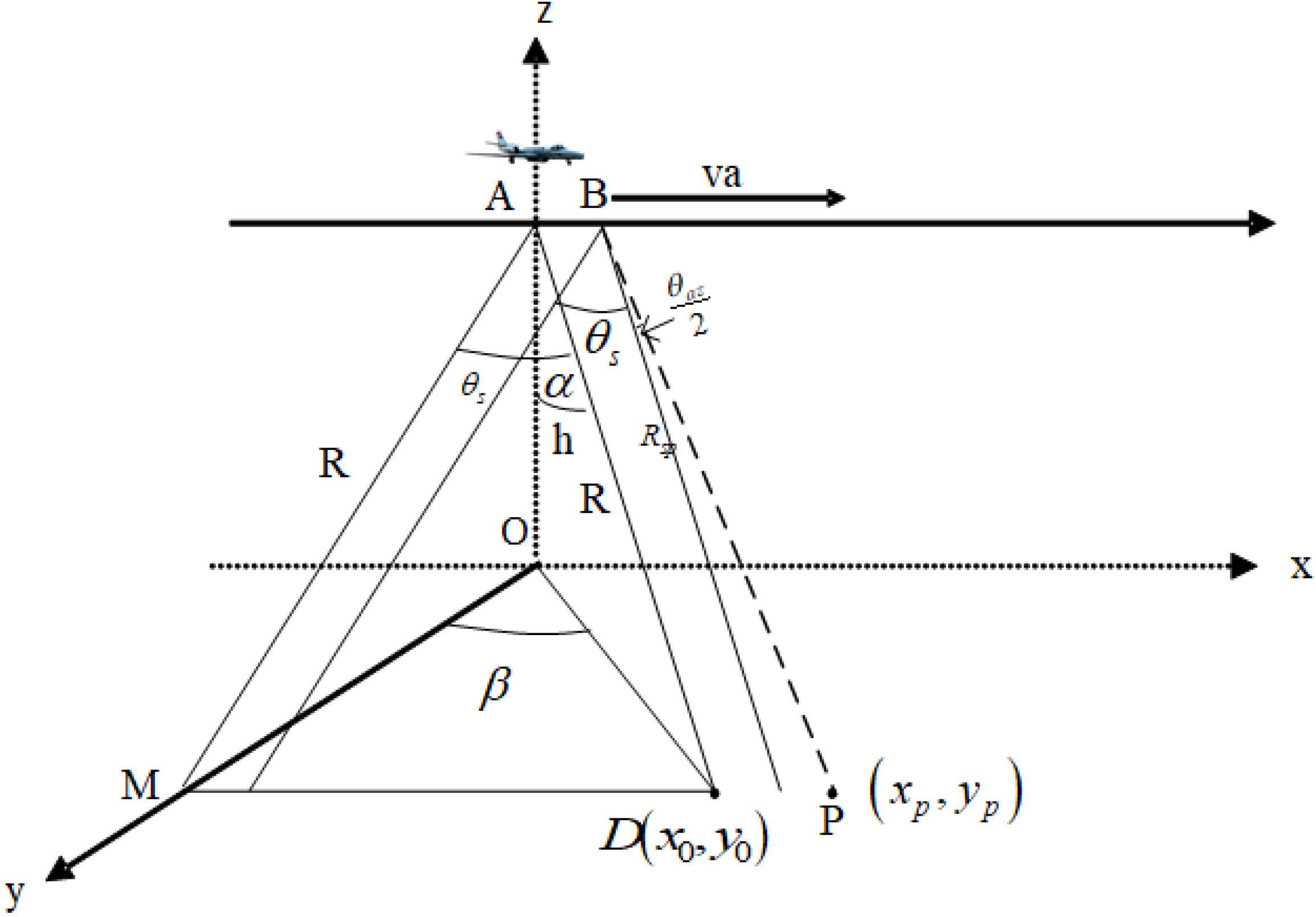
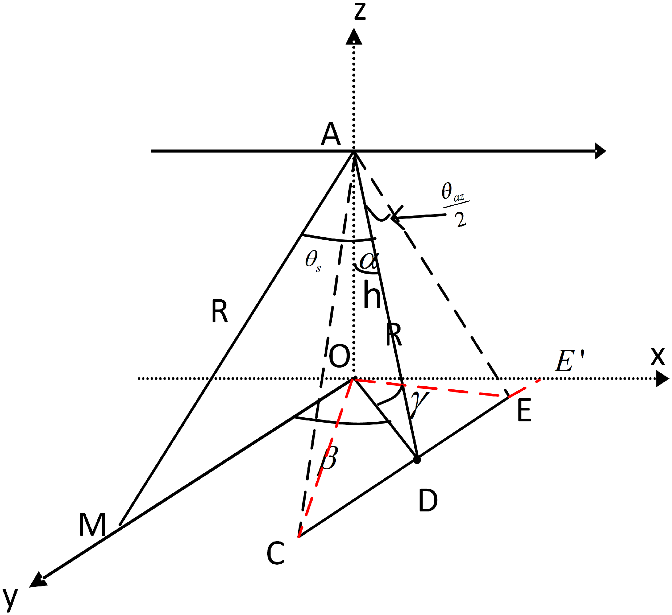
2. Observation Geometry
3. -k Imaging Algorithm of the Squint SAR
3.1. The Two-Dimensional Constraints of the Squint Angle on the Antenna Beam
3.1.1. Constraints of the Beam Width at a Certain Elevation and Squint Angle on the Observation Range in the Range Direction
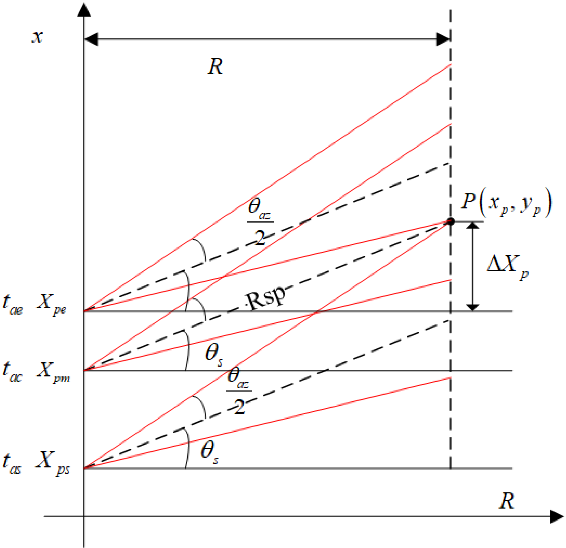
3.1.2. Constraints of Azimuth Beam Width and Squint Angle on Observing Range in Flight
3.1.3. Constraints Among Squint Angle, Beam Width at a Certain Elevation and Beam Width for a Certain Azimuth
3.2. Analysis of Signal Characteristics
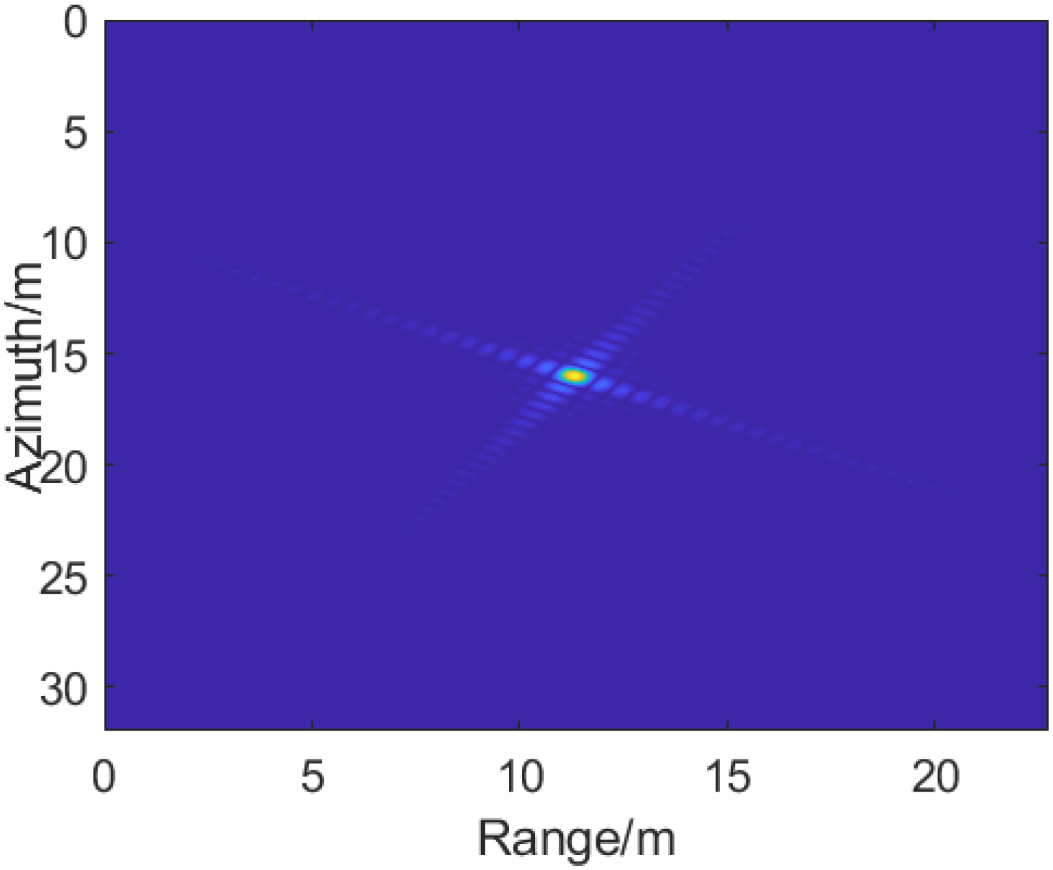
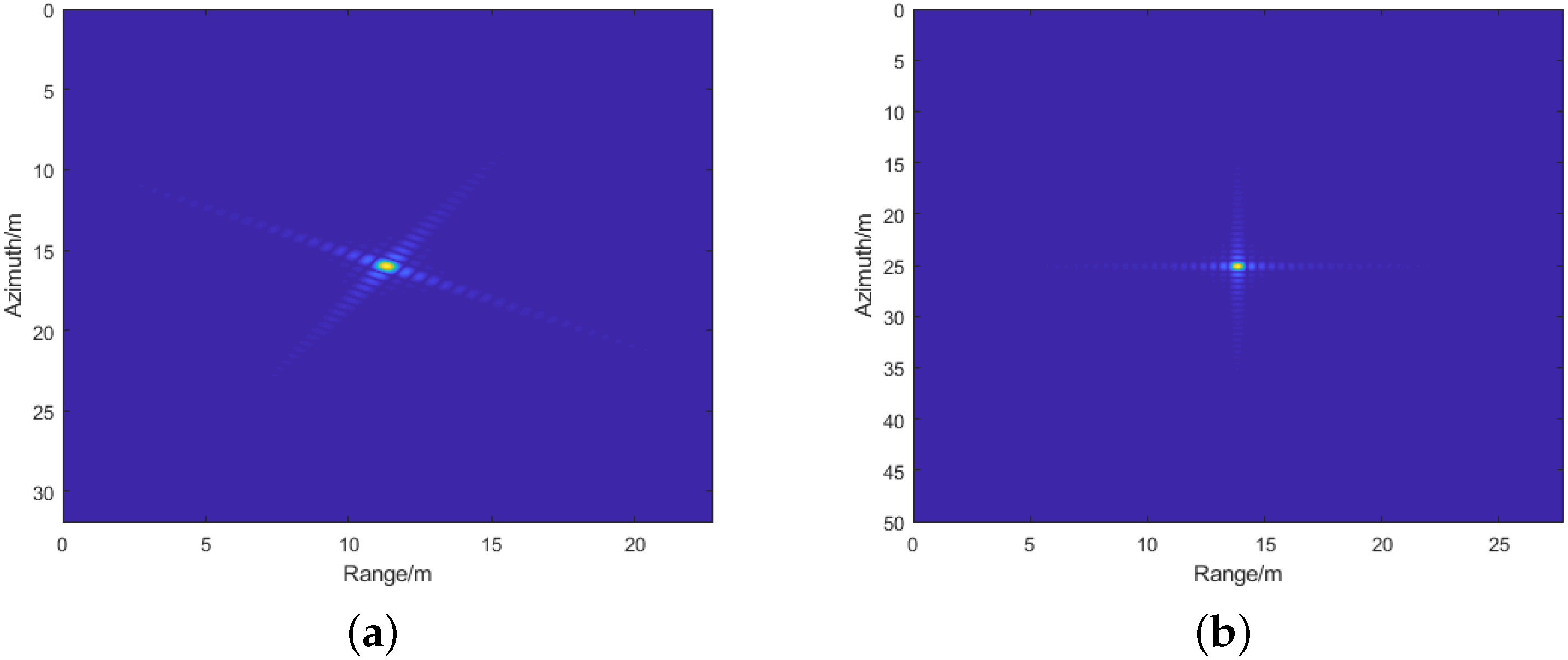
Performance Analysis of Point Target
- (1)
- Firstly, extract the point target from the two-dimensional SAR image;
- (2)
- Then, perform 16-fold interpolation of the image;
- (3)
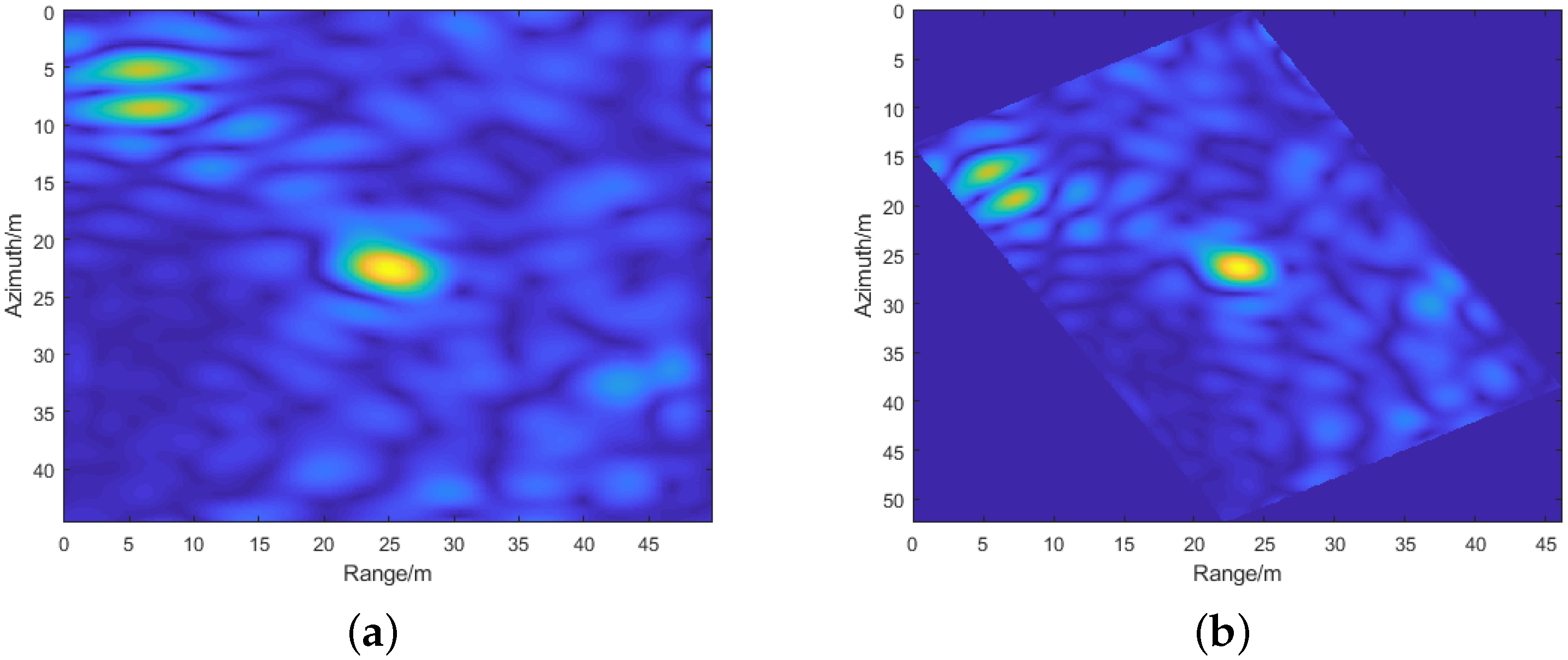
- Rotate the interpolated point target at an angle of . The rotation process is as follows:
- (a)
- (b)
- Rotate the coordinate system and determine the range of coordinates after rotation. If the number of sampling points in the range and azimuth directions of the captured, unrotated image is and , respectively, then the coordinates in the range and azimuth directions before rotation can be expressed as R and x, respectively:
- (c)
- Normalize the coordinates after rotation. The matrix composed of discrete samplings before rotation is uniformly sampled, but the corresponding coordinate points after rotation may no longer be uniformly spaced. Therefore, coordinate homogenization and image interpolation need to be carried out based on the coordinate distribution after rotation. The coordinates after homogenization are and , respectively.
- (i)
- Calculate the required number of samplings based on the new sampling interval and coordinate range after coordinate rotation:
- (ii)
- Reset the coordinates:
- (d)
- For image interpolation, based on the two-dimensional coordinate distribution of and before interpolation and the target image, interpolate the image values at and .
- (4)
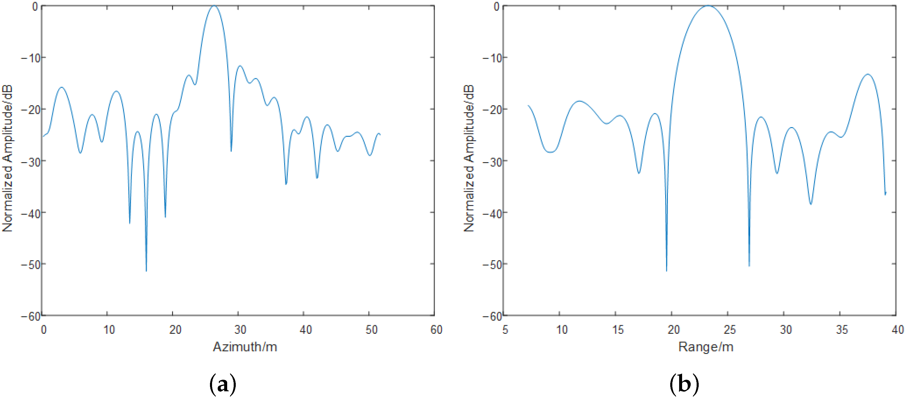
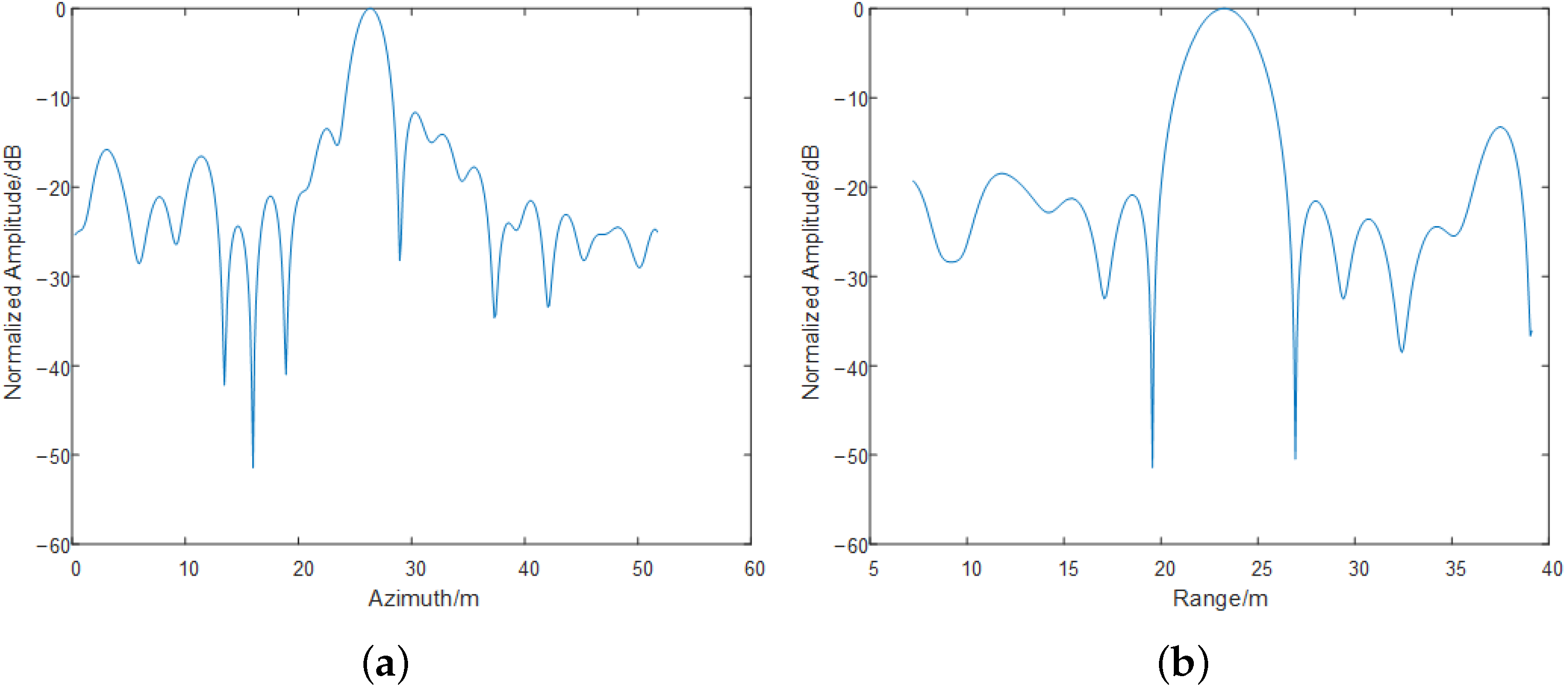
- Slice analysis of the rotated image in both the azimuth and distance directions should be performed.
3.3. Two-Dimensional Position Offset Analysis
3.3.1. Azimuth Position Offset and Correction
3.3.2. Range Position Offset and Correction
3.4. Diagram of the Algorithm
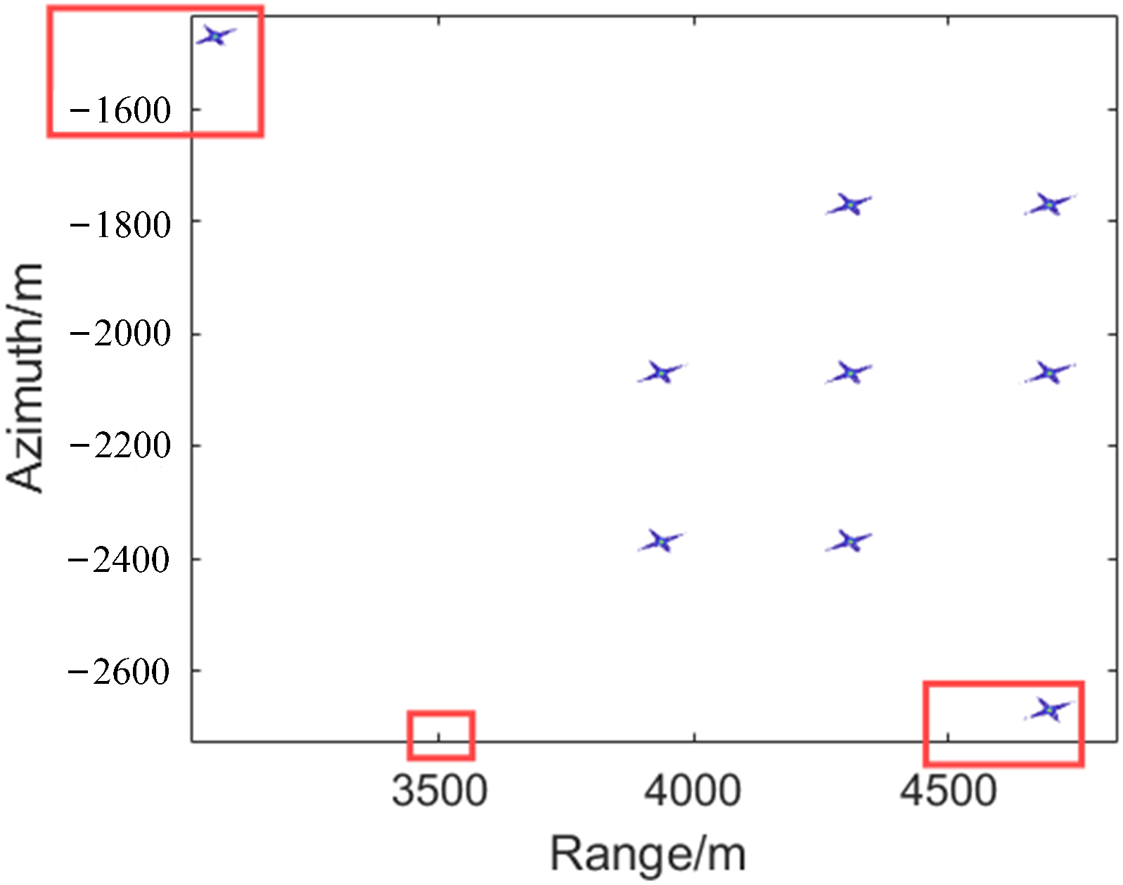
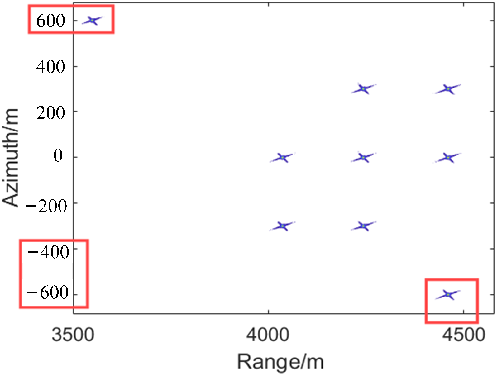
3.5. Simulation Experiments
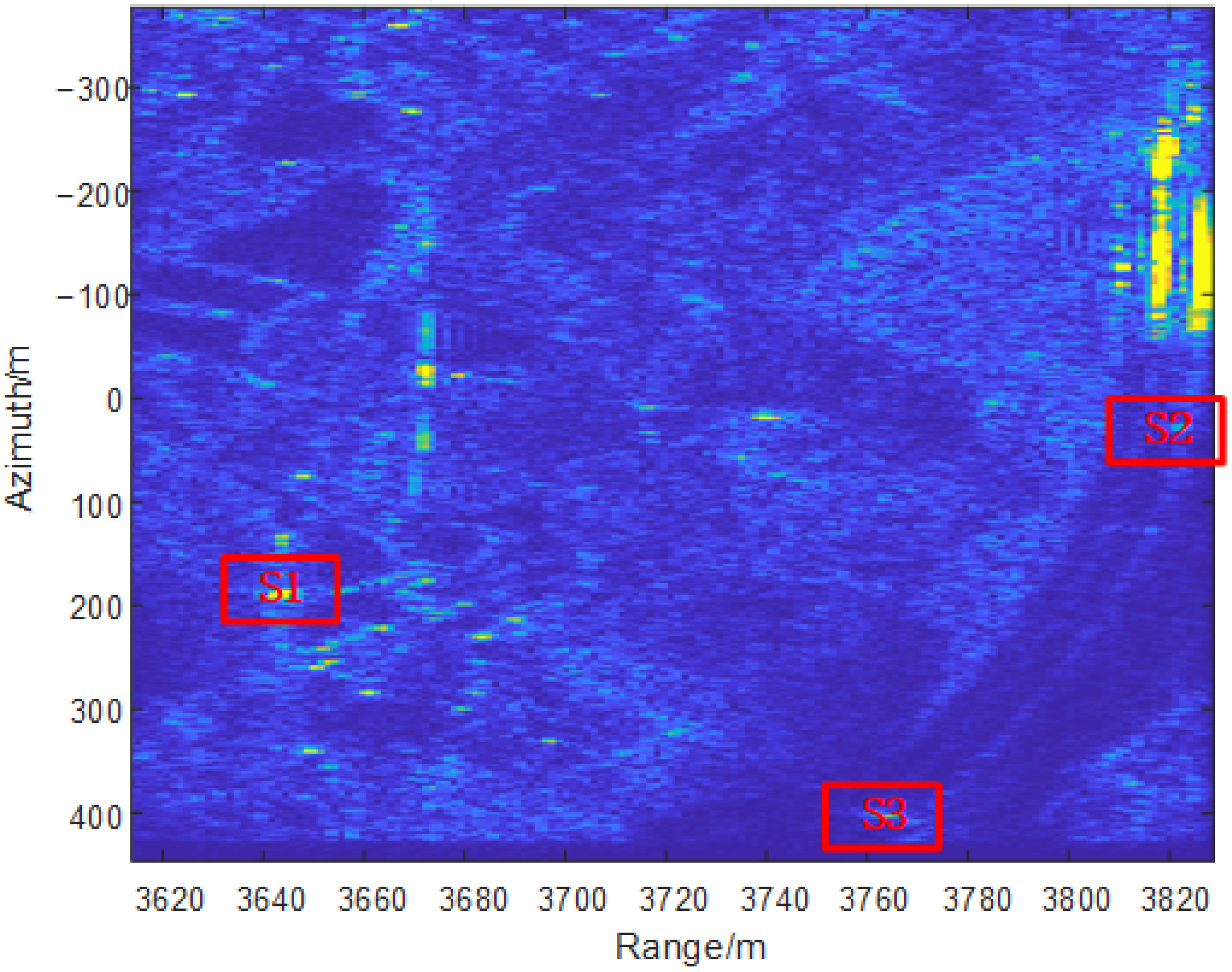
3.6. Experiment Results
4. Discussion
5. Conclusions
Author Contributions
Funding
Data Availability Statement
Conflicts of Interest
References
- Fornaro, G.; Sansosti, E.; Lanari, R.; Tesauro, M. Role of Processing Geometry in SAR Raw Data Focusing. IEEE Trans. Aerosp. Electron. Syst. 2002, 38, 441–454. [Google Scholar] [CrossRef]
- Brown, W.M. Synthetic Aperture Radar. Encycl. Phys. Sci. Technol. 1967, AES-3, 451–465. [Google Scholar] [CrossRef]
- Semenova, K. Real-time algorithm for the front-side-looking SAR. In Proceedings of the International Radar Symposium, Krakow, Poland, 10–12 May 2016. [Google Scholar]
- Jancco-Chara, J.; Palomino-Quispe, F.; Coaquira-Castillo, R.J.; Herrera-Levano, J.C.; Florez, R. Doppler Factor in the Omega-k Algorithm for Pulsed and Continuous Wave Synthetic Aperture Radar Raw Data Processing. Appl. Sci. 2024, 14, 320. [Google Scholar] [CrossRef]
- Xu, G.; Zhang, B.; Yu, H.; Chen, J.; Xing, M.; Hong, W. Sparse Synthetic Aperture Radar Imaging From Compressed Sensing and Machine Learning: Theories, applications, and trends. IEEE Geosci. Remote Sens. Mag. 2022, 10, 32–69. [Google Scholar] [CrossRef]
- Zhou, Y.; Wang, W.; Chen, Z.; Wang, P.; Zhang, H.; Qiu, J.; Zhao, Q.; Deng, Y.; Zhang, Z.; Yu, W.; et al. Digital Beamforming Synthetic Aperture Radar (DBSAR): Experiments and Performance Analysis in Support of 16-Channel Airborne X-Band SAR Data. IEEE Trans. Geosci. Remote Sens. 2020, 59, 6784–6798. [Google Scholar] [CrossRef]
- Wang, Z.; Wang, B.; Xiang, M.; Hu, X.; Song, C.; Wang, S.; Wang, Y. A Coherence Improvement Method Based on Sub-Aperture InSAR for Human Activity Detection. Sensors 2021, 21, 1424. [Google Scholar] [CrossRef] [PubMed]
- Semenova, K.I.; Shelevytsky, I.V.; Yanovsky, F.J. Front-side-looking SAR imaging. In Proceedings of the 13th International Radar Symposium, Warsaw, Poland, 23–25 May 2012. [Google Scholar]
- Hu, R.; Rao, B.S.M.R.; Murtada, A.; Alaee-Kerahroodi, M.; Ottersten, B. Automotive Squint-Forward-Looking SAR: High Resolution and Early Warning. IEEE J. Sel. Top. Signal Process. 2021, 15, 904–912. [Google Scholar] [CrossRef]
- Liu, B.; Liu, C.; Wang, Y. A new approach for SAR baseband Doppler centroid estimation. In Proceedings of the Global Intelligence Industry Conference (GIIC 2018), Beijing, China, 21–23 May 2018; Volume 10835, pp. 233–238. [Google Scholar]
- Yang, J.; Liu, C.; Wang, Y. Adaptive Doppler centroid estimation algorithm of airborne SAR. IEICE Electron. Express 2012, 9, 1135–1140. [Google Scholar] [CrossRef]
- Li, W.; Yang, J.; Wu, J.; Huang, Y.; Kong, L. An adaptive iterative scheme of Doppler centroid estimation for bistatic forward-looking SAR. In Proceedings of the 2010 IEEE Radar Conference, Arlington, VI, USA, 10–14 May 2010; pp. 262–265. [Google Scholar]
- Lee, Y.C.; Tsai, P.Y.; Lee, S.Y. Doppler centroid estimation with quality assessment for real-time SAR Imaging. In Proceedings of the 2020 Asia-Pacific Signal and Information Processing Association Annual Summit and Conference (APSIPA ASC), Auckland, New Zealand, 7–10 December 2020; pp. 36–40. [Google Scholar]
- Madsen, S.N. Estimating the Doppler centroid of SAR data. IEEE Trans. Aerosp. Electron. Syst. 1989, 25, 134–140. [Google Scholar] [CrossRef]
- Long, T.; Liu, L.; Ding, Z. Strategy of Doppler centroid estimation in synthetic aperture radar. IET Radar Sonar Navig. 2011, 5, 279–287. [Google Scholar] [CrossRef]
- Li, Z.; Xing, M.; Liang, Y.; Gao, Y.; Chen, J.; Huai, Y.; Zeng, L.; Sun, G.C.; Bao, Z. A Frequency-Domain Imaging Algorithm for Highly Squinted SAR Mounted on Maneuvering Platforms With Nonlinear Trajectory. IEEE Trans. Geosci. Remote Sens. 2016, 54, 4023–4038. [Google Scholar] [CrossRef]
- Yeo, T.S.; Tan, N.L.; Zhang, C.B.; Lu, Y.H. A new subaperture approach to high squint SAR processing. IEEE Trans. Geosci. Remote Sens. 2001, 39, 954–968. [Google Scholar]
- Shu, L.; Ying, W.; Yigong, Z. Exact analysis of the azimuth resolution characters of squint SAR. J. Syst. Eng. Electron. 2004, 15, 502–506. [Google Scholar]
- Li, Y. The Imaging Techniques of Missile-Borne Synthetic Aperture Radar. Ph.D. Thesis, National University of Defense Technology, Changsha, China, 2008. [Google Scholar]
- Liu, Y.; Liu, X.; Yuan, L.; Zeng, G.; Lv, H. Research on geometric correction in forward squint SAR imaging. Aerosp. Electron. Warf. 2023, 39, 13–18. [Google Scholar] [CrossRef]


| Parameter | Value | Parameter | Value |
|---|---|---|---|
| Radar center frequency (GHz) | 9.6 | PRF (Hz) | 470 |
| Scene center slant range (km) | 4.24 | Azimuth beam (°) | 2 |
| Scene center slant range (km) | 4.24 | Azimuth beam (°) | 2 |
| Radar initial position (km) | −3.36 | Velocity (m/s) | 150 |
| Transmitted bandwidth (MHz) | 280 | Pulse width (μs) | 5 |
| P1 | P2 | P3 | P4 | P5 | P6 | P7 | P8 | P9 | |
|---|---|---|---|---|---|---|---|---|---|
| Range (m) | 3549 | 4242.6 | 4459.8 | 4036.1 | 4242.6 | 4459.8 | 4036.1 | 4242.61 | 4459.8 |
| Azimuth (m) | 600 | 300 | 300 | 0 | 0 | 0 | −300 | −300 | −600 |
| Original Algorithm | Proposed Algorithm | |||
|---|---|---|---|---|
| (Range, Azimuth) | P1 (3549, 600) | P5 (4242.6, 0) | P1 | P5 |
| Position (m) | (2959, −1469) | (4320, −2068) | (3549, 600.3) | (4243, 0) |
| ISLR (dB) | (−11.01, −11.05) | (−11.01, −11.05) | (−11.05, −11.04) | (−11.05, −11.04) |
| PSLR (dB) | (−13.27, −13.27) | (−13.27, −13.27) | (−13.26, −13.27) | (−13.26, −13.27) |
| Resolution (m) | (0.48, 0.42) | (0.48, 0.42) | (0.48, 0.42) | (0.48, 0.42) |
| Parameter Name | Value |
|---|---|
| Radar center frequency (GHz) | 1.6 |
| Effective radar velocity (m/s) | 150 |
| PRF (Hz) | 70 |
| Transmitted bandwidth (MHz) | 50 |
| Squint angle (°) | 30 |
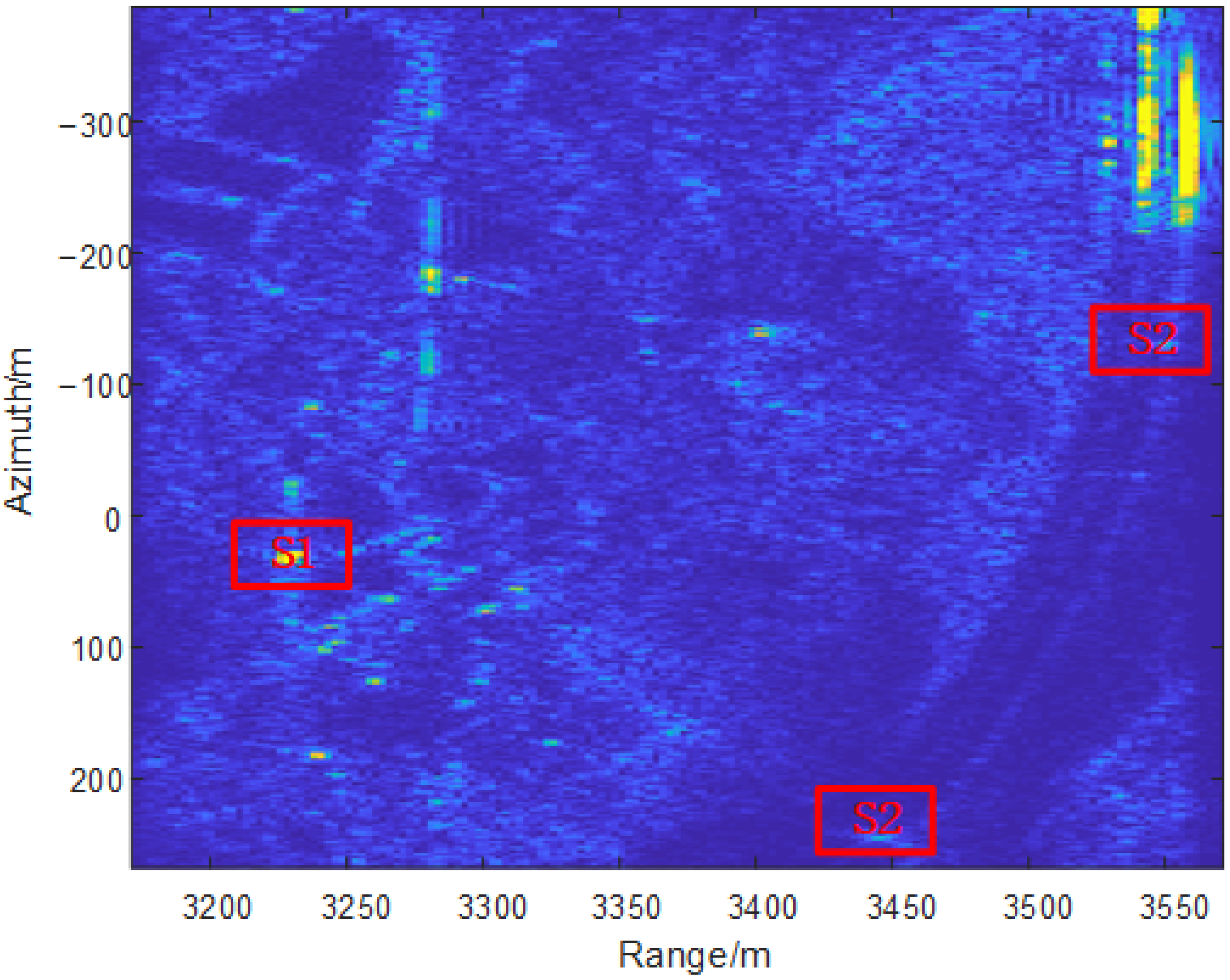
| Coordinates/Area | S1 | S2 | S3 |
|---|---|---|---|
| Reference Range/m | 3644 | 3822 | 3765 |
| Reference Azimuth/m | 187.2 | 27.2 | 400.5 |
| Corrected Range/m | 3643 | 3822 | 3764 |
| Corrected Azimuth/m | 187 | 28.7 | 401.8 |
| Uncorrected Range/m | 3228 | 3551 | 3443 |
| Uncorrected Azimuth/m | 30.3 | −130.8 | 245.2 |
Disclaimer/Publisher’s Note: The statements, opinions and data contained in all publications are solely those of the individual author(s) and contributor(s) and not of MDPI and/or the editor(s). MDPI and/or the editor(s) disclaim responsibility for any injury to people or property resulting from any ideas, methods, instructions or products referred to in the content. |
© 2025 by the authors. Licensee MDPI, Basel, Switzerland. This article is an open access article distributed under the terms and conditions of the Creative Commons Attribution (CC BY) license (https://creativecommons.org/licenses/by/4.0/).
Share and Cite
Wang, S.; Song, C.; Wang, B.; Chen, J.; Yang, L.; Huang, Z. Two Dimensional Position Correction Algorithm for High-Squint Synthetic Aperture Radar in Wavenumber Domain Algorithm. Remote Sens. 2025, 17, 1015. https://doi.org/10.3390/rs17061015
Wang S, Song C, Wang B, Chen J, Yang L, Huang Z. Two Dimensional Position Correction Algorithm for High-Squint Synthetic Aperture Radar in Wavenumber Domain Algorithm. Remote Sensing. 2025; 17(6):1015. https://doi.org/10.3390/rs17061015
Chicago/Turabian StyleWang, Shuai, Chen Song, Bingnan Wang, Jie Chen, Lixia Yang, and Zhixiang Huang. 2025. "Two Dimensional Position Correction Algorithm for High-Squint Synthetic Aperture Radar in Wavenumber Domain Algorithm" Remote Sensing 17, no. 6: 1015. https://doi.org/10.3390/rs17061015
APA StyleWang, S., Song, C., Wang, B., Chen, J., Yang, L., & Huang, Z. (2025). Two Dimensional Position Correction Algorithm for High-Squint Synthetic Aperture Radar in Wavenumber Domain Algorithm. Remote Sensing, 17(6), 1015. https://doi.org/10.3390/rs17061015