Article

Temporal Upscaling of Agricultural Evapotranspiration with an Improved Evaporative Fraction Method

1
College of Water Conservancy and Hydropower Engineering, Sichuan Agricultural University, Yaan 625014, China
2
State Key Laboratory of Water Resources and Hydropower Engineering Science, Wuhan University, Wuhan 430072, China
3
College of Hydraulic Science and Engineering, Yangzhou University, Yangzhou 225009, China
*
Author to whom correspondence should be addressed.
Remote Sens. 2025, 17(6), 1016; https://doi.org/10.3390/rs17061016
Submission received: 25 January 2025 / Revised: 9 March 2025 / Accepted: 10 March 2025 / Published: 14 March 2025

Abstract

:
Evapotranspiration (ET) is a crucial parameter for agricultural management and the hydrologic cycle, and instantaneous satellite images are the primary data source for regional ET. The constant evaporative fraction method (EFO) is a common approach for converting short-time ET (ETst) to daily ET (ETday). However, EFO has some limitations due to simple assumptions, including the following: the short-time evaporative fraction (EFst) equals the daily evaporative fraction (EFday). This study proposed an improved evaporative fraction method (EFI) through theoretical derivation and data analysis without additional data requirements, enabling the accurate upscaling of ETst to ETday. The vapor pressure deficit and available energy were considered in EFI to describe the main effect factor and estimate the deviation between EFst and EFday, defining the deviation coefficient and potential deviation between EFst and EFday. EFI was tested through four aspects: different agricultural systems, various sites, two growth stages, and different sources of EFst, comparing estimated ETday from EFI and measured ETday. EFI reduced the mean absolute percentage error (MAPE) of ETday estimation from 23% to 16% when EFst is derived from measured data compared to EFO. Similarly, the MAPE of ETday estimation reduced from 38% to 31% when EFst is derived from a remote sensing model (Surface Energy Balance Algorithm for Land, SEBAL). EFI performs better during the growing period than the fallow season, providing critical information for irrigation practices. Crop type is not a main control factor for the relationship between η (ratio between VPD and Rn-G) and EFst, and EFI is adaptable to various agricultural systems. The encouraging results of EFI in different scenarios demonstrate its accuracy and robustness. Therefore, EFI is anticipated to upscale EFst to EFday, generating a more accurate ET on a regional scale through remote sensing technology.

Graphical Abstract

1. Introduction

Some empirical models were proposed based on satellite images to simulate the daily ET (ETday). Jackson et al. [1] estimated the ETday via the temperature difference between canopy and air, which is simple but requires measured data to calibrate. Price [2,3] deduced the relationship between ETday and the instantaneous surface temperature from the heat flow equation. Based on studies of Seguin and Itier [4], Carlson et al. [5] introduced the average bulk conductance for daily integrated sensible heat flux and correction for nonneutral static stability and established a simplified method for integrating ETday. These empirical methods provide excellent ET estimation for specific conditions and areas. Unfortunately, these methods have limited applicability in ETday estimation because some parameters vary for different regions.
Instantaneous ET was calculated more and more accurately with the development of remote sensing technology and theory, and it was extrapolated according to the similarity between the diurnal course of ET and that of other components of the surface energy balance [6]. Jackson et al. [7] assumed the diurnal course of ET follows the diurnal course of radiation for cloud-free days, depicting it with a sine function. However, the practicability of this method was restricted by the topography, weather conditions, and time of instantaneous EF. According to the self-preservation of the reference ET fraction, Allen et al. [8] and Tasumi et al. [9] upscaled the instantaneous ET to ETday through the ratio of actual ET and alfalfa reference ET. The surface resistance method was another excellent approach for ETday estimation [10], using the instantaneous surface resistance to replace the daily surface resistance, representing a good performance. However, determining the parameters is a challenge, therefore constraining the application.
The evaporative fraction was defined as the latent heat flux divided by the available energy flux [11]. The constant evaporative fraction during a day was a crucial hypothesis in the constant evaporative fraction method (EFO) [6], which was widely applied for converting the short-time ET to ETday [12,13,14,15,16,17]. However, some studies [18,19,20,21,22] proved that the ETday would be underestimated or overestimated when the EFO was adopted. Many efforts [23,24,25,26] have been made to improve the calculation accuracy, considering more circumstance factors. These methods have acquired acceptable results in different regions, but the additional data input might constrain the application.
Based on the deficiencies of previous methods, an improved evaporative fraction method (EFI) is proposed, considering vapor pressure deficit (VPD, expressed by air temperature and surface vapor pressure) and available energy (τ). The VPD and τ are essential parameters in the short-time EF calculation from remote sensing models, so EFI does not require more data than EFO. The objectives of this study were (1) to develop an improved evaporative fraction method without additional data requirements; (2) to test this method in different agricultural systems and for different sites; and (3) to assess the performances of EFI when the short-time EF is obtained from a remote sensing model and ground-measured data.

2. Materials and Methods

2.1. Experiment and Data Collection

2.1.1. Eddy Flux and Micrometeorological Measurements

The field experiment was conducted from 2017 to 2019 in a paddy field (28.45°N, 116.01°E) located in south China where the mean annual temperature is 18.1 °C and annual precipitation is over 1600 mm. The early paddy rice was seeded in late April and harvested in mid-July, followed by transplantation of late paddy rice in late July and late paddy rice harvesting in late October or early November. The paddy rice field flooded during all rice growth periods besides the late tillering and late maturity growth stages (dry condition).
An eddy covariance (EC) system was installed in the center of the paddy field to observe the energy flux, equipped with a fast response 3D sonic anemometer (WindMasterPro, Gill Instruments Inc., Lymington, UK), an open path H2O gas analyzer (LI-7500A, Li-COR Biosciences Inc., Lincoln, NE, USA), and a data logger (LI-7550, Li-COR Biosciences Inc., Lincoln, NE, USA). The EC system and meteorological sensors were installed at 2.5 m above ground. The meteorological data were collected with a meteorological system, including an air temperature and humidity sensor (HMP155A, Vaisala Instruments Inc., Helsinki, Finland) and a net radiation sensor (NR-lite2, Kipp&Zonen Instruments Inc., Delft, The Netherlands). Meanwhile, soil moisture and temperature sensors (ML2x, Delta-T Devices Inc., Burwell, UK) and a soil heat flux plate (HFP01, Hukseflux Instruments Inc., Delft, The Netherlands) were buried at a depth of 5 cm, and the daily water depth was obtained by rulers.
To evaluate the performance of EFI, the short-time EF (EFst) from EC systems and the Surface Energy Balance Algorithm for Land (SEBAL) model were used to calculate the daily ET, respectively. We initially collected EC data from all agricultural monitoring systems available on the FLUXNET community (https://fluxnet.org (accessed on 12 November 2024)) and AsiaFlux (http://asiaflux.net (accessed on 14 November 2024)). However, several sites were excluded due to either incomplete records of critical parameters (e.g., net radiation data) or insufficient ancillary information regarding crop types and cultivation schedules. Following rigorous data quality screening and metadata completeness verification, 15 representative sites (Figure 1 and Appendix A) were ultimately selected. The EC systems were installed in agricultural systems, including winter wheat, winter barley, spring barley, soybean, cowpea, sugar beet, rapeseed, mustard, maize, paddy rice, potato fields, and orange orchard, and providers have preprocessed the flux data. The FLUXNET community and AsiaFlux provide 30 min or 60 min flux data, so the short-time data refers to hourly or half-hourly data for EC data analysis and instantaneous data for remote sensing data analysis in this study. In addition, the half-hourly data were aggregated to daily data, and the data processing procedures can be found in Wei et al. [27].

2.1.2. Remote Sensing Data Collection

For the ET estimation using remote sensing technology, many satellites (i.e., MODIS, Landsat, NOAA, Sentinel-2A) have been highly considered by researchers [28,29]. Although some sensors (i.e., WorldView series) can provide higher spatiotemporal resolution, the high price blocks its prevalence. This study adopted Landsat as the input of the remote sensing model, with a relatively high spatial resolution (30 m) and a long record (from 1987), which could be used for long-time monitoring. Quality bands of Landsat images were used to remove the bad pixels with bit arithmetic [30]. The Landsat images and digital elevation model datasets (DEM), which were used to correct the land surface temperature (Equation (D10)), with 30 m spatial resolution, were collected from the United States Geological Survey (https://www.usgs.gov/ (accessed on 28 November 2024)). The European Centre for Medium-Range Weather Forecasts Reanalysis v5 (ERA5) dataset was acquired from medium-range weather forecasts (http://www.ecmwf.int/ (accessed on 28 November 2024)), providing raster meteorological data (air temperature at 2 m, net radiation, and wind speed at 2 m) with hourly temporal resolution and 0.1° spatial resolution. Those datasets were used to calculate the EFst and ETday through remote sensing technology. All remote sensing raster data whose spatial resolution was not 30 × 30 m were resampled to 30 × 30 m using cubic interpolation [27].

2.2. Data Preprocessing

The raw data (10 Hz) from EC were processed with EddyPro software (Version 7.0.9), and the 30 min interval initial latent (LE) and sensible (H) heat flux were obtained. The low-quality data flagged by EddyPro was removed, which was influenced by rainfall, instrument malfunction, and other disturbances. Meanwhile, the data with a friction velocity lower than 0.15 m·s−1, which is unreliable [31], was also removed. ReddyProc, an online tool (https://www.bgc-jena.mpg.de/ (accessed on 15 November 2024)), was used for half-hour data gap-filling. The data from January to April 2019 were missing due to equipment failure. The difference between net radiation and soil heat flux (Rn-G) should be equal to turbulent energy (H + LE) according to the energy balance principle [32], and the Bowen ratio (β) was adopted to force energy balance closure [33]. For this method, the residual energy (Rn-G-LE-H) can be partitioned into additional H and LE depending on β. The sum of additional H or LE and original H or LE is the closed H or LE. The specific procedure can be found in Appendix B. The soil heat flux (G) calculation method was as follows:
G = G 0 + G s + G w
G s = Δ T s t d s ( ρ s C s + ρ w C w θ w )
G w = Δ T w t d w ρ w C w
where G0 is the measured data by soil heat flux plate, W·m−2; Gs and Gw represent changes in soil and water heat storage, respectively, W·m−2; ΔTs and ΔTw is the variation in soil and water temperature, respectively, K; ds is the depth of layer above soil heat flux sensors, 5 cm; dw is the water depth, cm; ρs is the soil dry bulk density, 1360 kg·m−3; ρw is water density, 1000 kg·m−3; θw is the soil water content; and Cs and Cw are the specific heat capacity for soil solid portion (840 J·kg−1·K−1) and water (4190 J·kg−1·K−1).

2.3. Improved Evaporative Fraction Method

The EFst equals the daily EF (EFday) according to the constant evaporative fraction method (EFO) [6], so ETday can be obtained from daily available energy (Rn-G) and EFst. Unfortunately, EF is not a constant intra-day, which is influenced by many factors [18,23]. Considering the effects of circumstance, the improved evaporative fraction method (EFI) was proposed, including three core procedures. (1) The main control factors of EF were analyzed according to Penman–Monteith. The deviation coefficient (δ) between EFst and EFday was defined as the main influence factors of EF. (2) The determination of the potential difference (Ω) between daily EFday and EFst. (3) The product of δ and Ω was defined as the deviation between EFday and EFst. Then, the EFday was obtained by finding the sum of the deviation and EFst. The specific procedure and flowchart of EFI are shown in Figure 2.

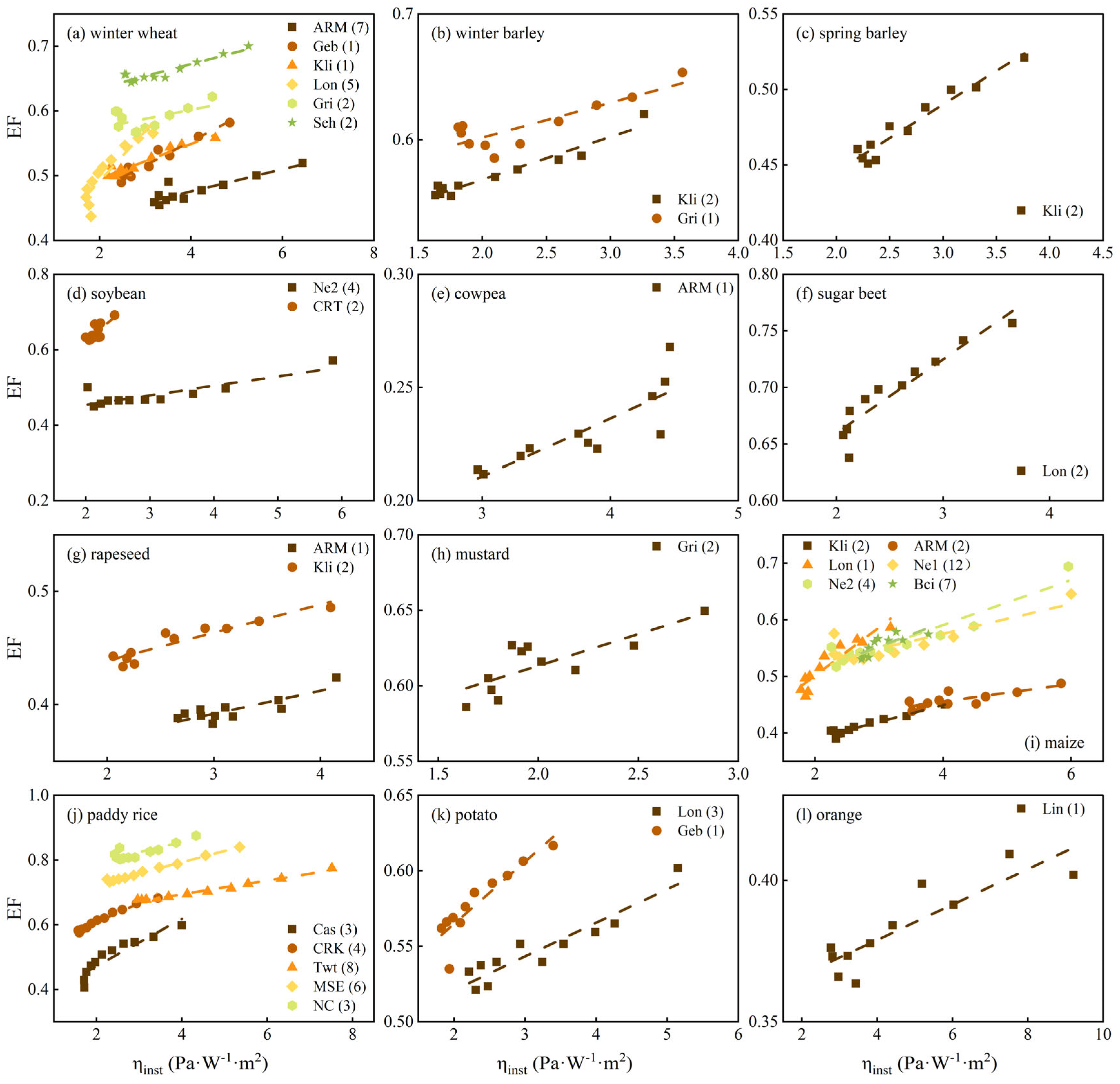
2.3.1. The Deviation Coefficient Between EFday and EFst

From the PM equation [33], EF can be described by a group of meteorological factors as follows.
L E = Δ ( R n G ) + c p ρ a e s e a r a Δ + γ ( 1 + r s r a )
E F = Δ Δ + γ ( 1 + r s r a ) + c p ρ a r a Δ + γ ( r a + r s ) × V P D R n G
where Δ represents the slope of the saturation vapor pressure curve, kPa·°C−1; cp represents the air-specific heat at constant pressure, kPa·°C−1; ρa is the air density, kg·m−3; es represents saturation vapor pressure, kPa; ea represents the actual vapor pressure, kPa; esea represents saturation vapor difference (VPD), kPa; ra represents the aerodynamic resistance, s·m−1; rs represents surface resistances, s·m−1; and γ is the psychrometric constant, kPa·°C−1. The intra-day γ, cp, and ρa would not change sharply [34], and so they are regarded as the constants in this study.
Given the EF stability (explained hereinafter) and satellite overpass time, the flux data from daytime (referring to 9:30–14:30 in this study) were analyzed. Meanwhile, the EFday of a certain location is estimated from the EFst of the location, so the subsequent variable analysis is conducted on the daytime (9:30–14:30) of the specific location, not the regional scale or a long period.
Many studies [35,36] have proven that rs varies with VPD, temperature, soil water content, and canopy structures. For a short time, the soil water content and canopy structures will not change sharply. Temperature is always associated with net radiation, and VPD was considered in the η (ratio between VPD). In a brief time frame, solar radiation is the key factor in rs [37], and the threshold of solar radiation controls the lowest rs. To be specific, rs will not decrease continuously when solar radiation reaches the threshold value (relatively high value) [38,39], so rs shows a stable value during the daytime. The target time of this study is cloud-free time when solar radiation is strong, and rs might be stable intra-daytime. Meanwhile, many studies [35,36,40,41] have proved that rs maintains a relatively stable value during the daytime for different crops and meteorological conditions. So, rs was regarded as a constant in this study.
The ra can be calculated with crop height and wind speed [34].
r a = ln ( z m d 0 z om ) ln ( z h d 0 z oh ) k 2 u z
d 0 = 0.667 h ;   z om = 0.123 h ;   z oh = 0.1 z m
where zm is the height of wind measurements; zh is the height of humidity measurements; d0 is the zero plant displacement height; zom is the roughness length governing momentum transfer; zoh is the roughness length governing the transfer of heat and vapor; k is the von Karman’s constant, 0.41 [34]; uz is the wind speed at height z; and h is the crop height. zm and zh would be the constant if the locations of the sensors were not disturbed by human or non-human factors. Meanwhile, the crop height will not change sharply in one day. So, ra is just influenced by wind speed during 9:30–14:30 in the same place. Bailey and Davies [42] have illustrated that the ET is insensitive to ra when the PM equation is applied to estimate the ET.
To achieve a tradeoff between model complexity and accuracy, the effect of wind speed (wind speed and ra during daytime were analyzed in Appendix C) on ra was not factored, and ra was treated as a constant throughout the daytime. Δ can be described by the air temperature, and es is a temperature variable. The influence of Δ fluctuation on EF is ignored during the day to simplify the calculation procedure, just considering one temperature variable: es.
While we acknowledge that ra and rs may vary in longer time scales, our analysis focused specifically on the stable daytime period, which justifies the assumption of constant ra and rs for this short time frame. In conclusion, although we recognize that these assumptions might introduce some uncertainties, they were made to simplify the model and reduce its complexity, while still capturing the key dynamics of evapotranspiration during the stable daytime period. So, Equation (5) can be rewritten as follows.
E F = d + k × η
d = Δ Δ + γ ( 1 + r s / r a ) ;   k = c p ρ a r a Δ + γ ( r a + r s ) ;   η = V P D R n G
where d and k are the constants of the EF function (Equation (8)); η is the variable of the EF function (Equation (8)). So, EF could be described by VPD and available energy (Rn-G, τ), as suggested in other studies [43,44,45]. For good operability and data accessibility, the deviation coefficient (δ) and potential deviation (Ω) between EFday and EFst were used to determine the deviation between EFday and EFst, which are explained hereinafter. So, the deviation coefficient (δ) was defined as the η relative deviation between daily and short time.
δ = η day η st η day
where subscript day and st represent the daily and short-time data (including instantaneous data, hourly data, and half-hourly data), respectively.

2.3.2. The Potential Deviation Between EFday and EFst

Potential deviation (Ω) is the possible error when the EFst is used to express EFday in the EFO. Ω should theoretically be the maximum EFday or EFst. Nevertheless, it is hard to say that the deviation maintains the maximum every moment and EFday is the target value, so we just use the EFst to describe the Ω. An adjustment coefficient (t) was introduced to depict the Ω for most conditions in one agricultural system, and Ω was defined as follows when EFst ≤ 1.
Ω = t E F st
where t represents the adjustment coefficient related to crop type and meteorology, analyzed hereinafter.

2.3.3. Daily EF

Given that the EFst during the daytime is relatively stable [6] and close to EFday [46,47], the EFst was retained in EFI, and the deviation between EFst and EFday needed to be determined to obtain a more accurate EFday through EFst.
Ω represents the possible maximum deviation between EFst and EFday, not the actual deviation between EFst and EFday, so the deviation coefficient (δ) was introduced to determine the relative deviation between EFst and EFday. The actual deviation between EFst and EFday could be described as the product of δ and Ω (Equation (12)).
The EFday from EFI was used to estimate the daily ET with ground-measured data and a remote sensing model (SEBAL, which needs to input the remote sensing images and conventional meteorological data, and the specific procedure and inputs can be found in Appendix D), respectively.
E F day = E F st + δ Ω
λ E T day = L E = E F day ( R n - G ) day
where λ is the latent heat of vaporization, 2.45 MJ·kg−1.

2.4. Validation Methods
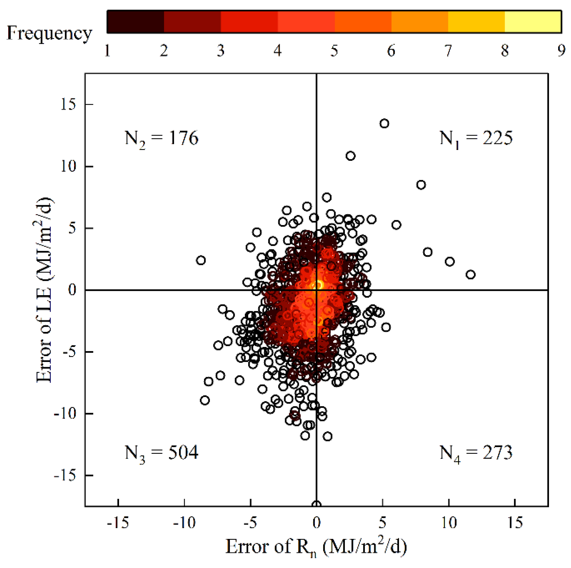
To assess the performance of EFI, two sources of short-time EF were adopted: ground-measured data (hourly or half-hourly EF from ground-measured data) and a remote sensing model (instantaneous EF from SEBAL). The averaged ET derived from a 3 × 3 pixel window centered on the flux tower (covering its most flux footprint area) was directly compared with the eddy covariance (EC) measurements to evaluate the consistency between remote sensing estimates and ground-based observations [27].
The root mean squared error (RMSE), mean absolute percentage error (MAPE), determination correlation (R2), and agreement index (AI) [48,49] were adopted in this study to evaluate the EFI performance in different situations.
R M S E = 1 N ( Y i f ( x i ) ) 2
M A P E = 1 N Y i f ( x i )
R 2 = 1 ( Y i f ( x i ) ) 2 ( Y i Y ¯ ) 2
A I = 1 Y i f ( x i ) 2 Y i Y ¯ + f ( x i ) Y ¯ 2
where Yi is the measured data, f (xi) is the estimated value, N is the number of data, and Y ( ) is the mean measured value.

3. Results

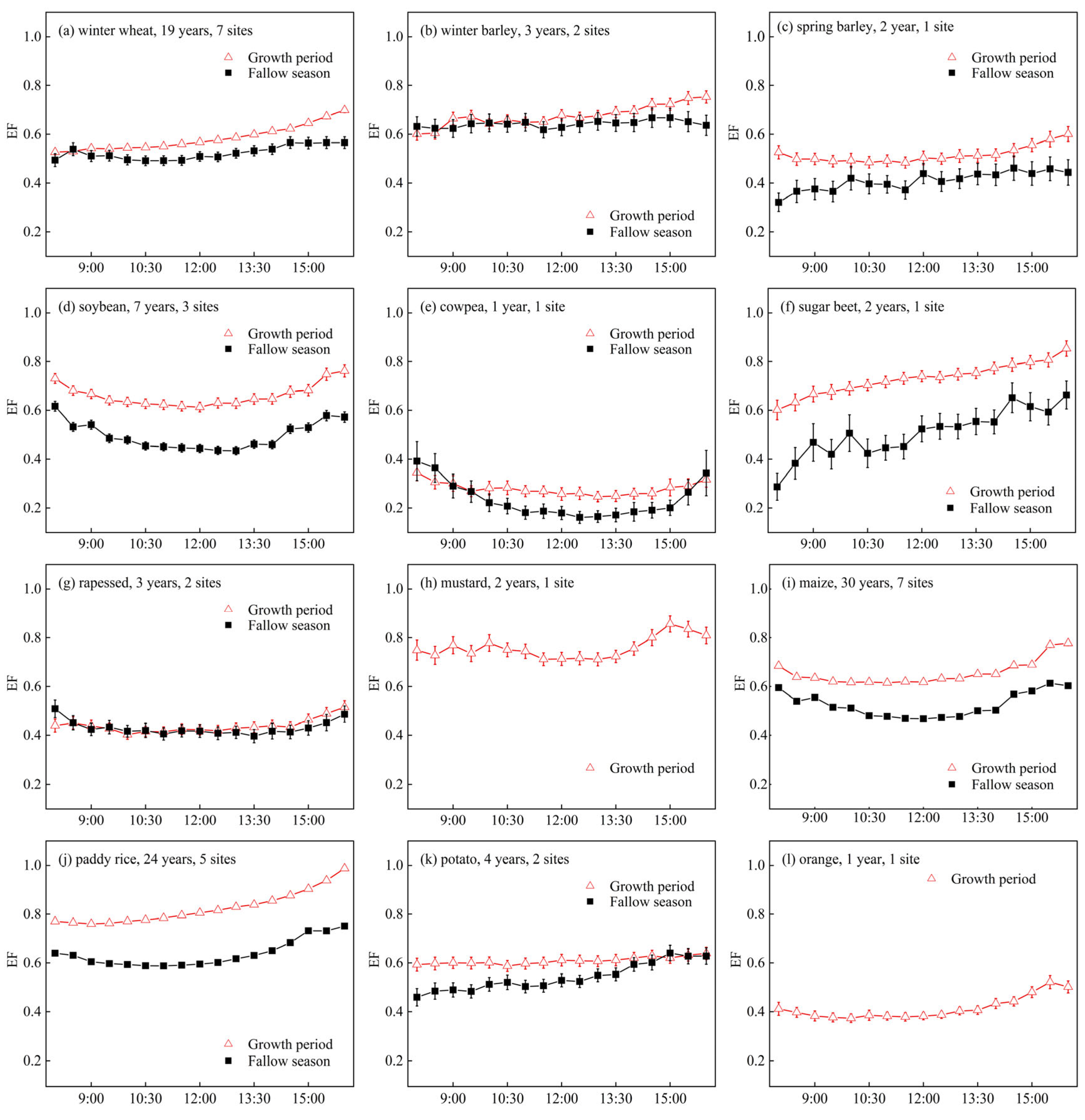
3.1. Measured Diurnal Evaporative Fraction for Agricultural Systems

The low Rn-G, amplifying the relative sensitivity of evapotranspiration (ET) to rapid variations in soil moisture, VPD, and turbulent mixing, would cause wild fluctuating EF [50,51], and so EFst from 8:00 to 16:00 (relatively high Rn-G) from EC datasets were analyzed. EF is more affected by the soil water condition (irrigation practice) and available energy (hard to describe quantitatively with limited sites), so the EF variation was displayed according to crop types (Figure 3). Besides rapeseed (Brassica napus subsp. napus), the other crops have higher EFst during the growth period (GP) than during the fallow season (FS). An adequate water supply (e.g., irrigation and precipitation) and enough available energy resulting in higher evaporation and transpiration during GP might be the reason for higher EF [23,25]. The rapeseed is planted in DE_Kli and US_ARM stations, the crop rotation land, and the FS always concentrates on July to October when the radiation (Rn is 104 W·m−2) and precipitation (2.8 mm·d−1) are enough. So, the evaporation condition is favorable for rapeseed fields even during FS. That is why the EFst is similar during FS and GP. The EFst of paddy rice fields is higher than that of upland fields because of the ample water supply.
EF is the ratio of LE and Rn-G, and EFst was more stable and lower at midday than at other times when the Rn-G is typically the largest. With the decrease of Rn-G (denominator of EF), the EFst becomes sensitive to Rn-G and increases gradually. Due to the data quality limitation, only 80 days of data are available during FS of sugar beet, and the time span is from November to April. So, the EFst shows a more significant fluctuation during this period. Besides the FS of sugar beet, EFst between 9:30 and 14:30 is stable for other crops, and the lower Rn-G (denominator of EF) during other times might lead to greater deviation between short-time and daily EF [46,52]. Meanwhile, the overpass time for Landsat is also between 9:30 and 14:30. Every half hour (or hour), EFst between 9:30 and 14:30 was adopted in the following analysis for a reliable result.

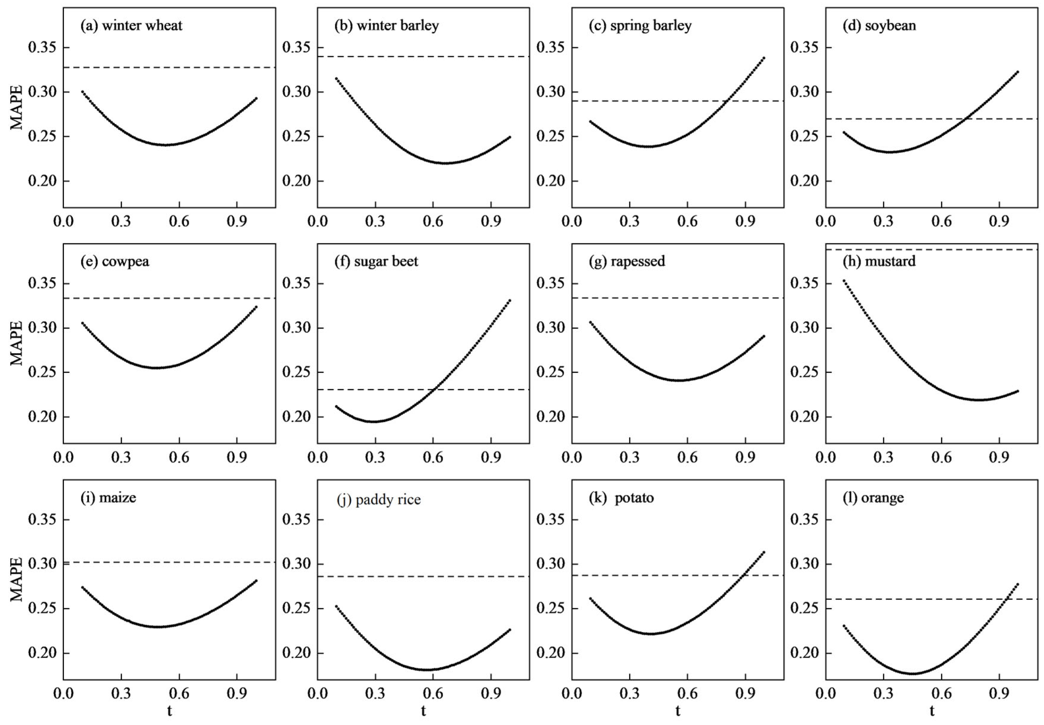
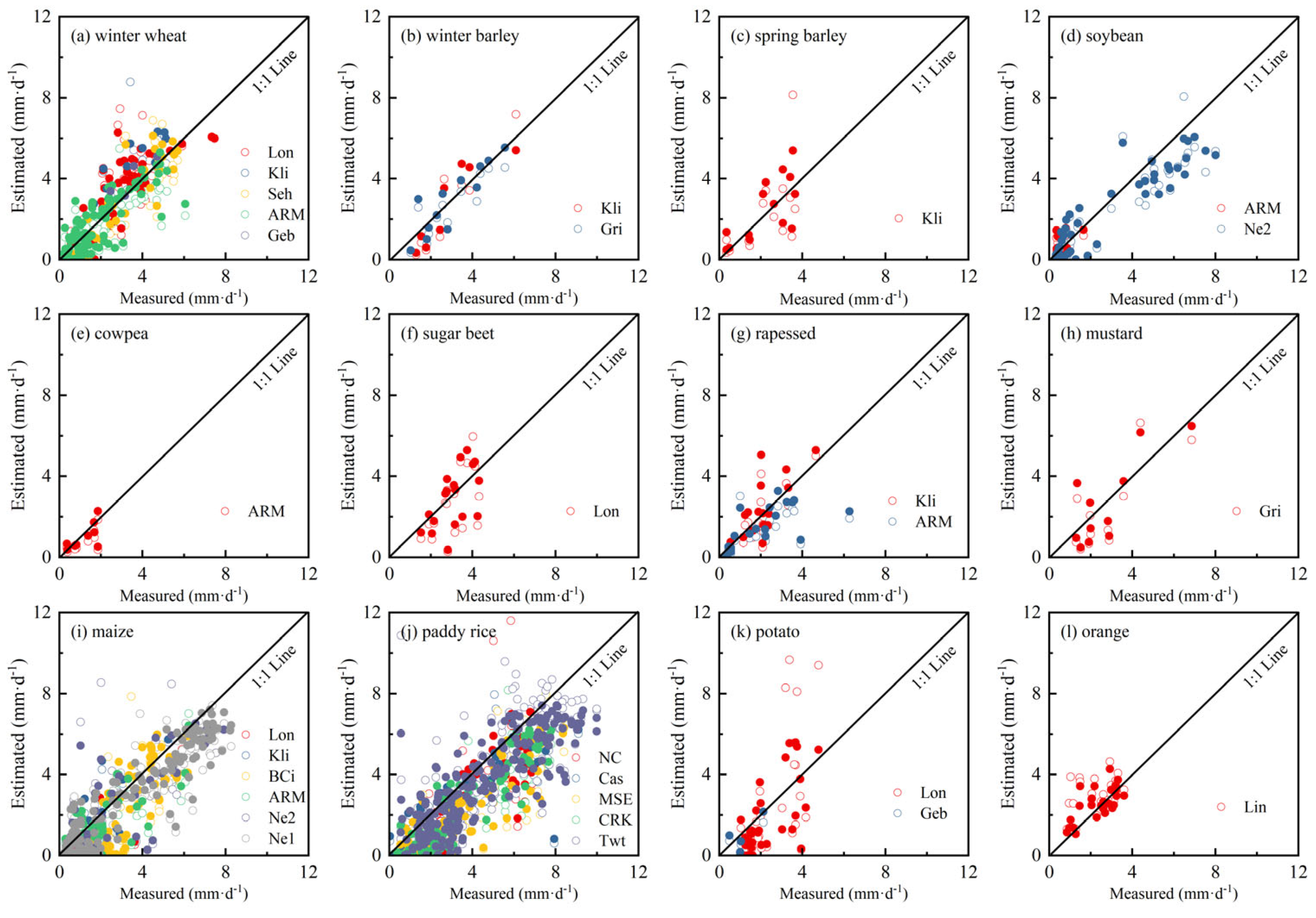
3.2. Daily EF from the Improved Evaporative Fraction Method

Every half-hourly and hourly EF during 9:30–14:30 from EC was upscaled to daily EF (00:00–23:59) through the improved evaporative fraction method (EFI) in different agriculture systems. To determine the appropriate adjustment coefficient of Ω (t), MAPE between upscaled EF with EFI and measured daily EF were analyzed, with initial t values 0.1 and 0.01 as the step size. The MAPE shows a similar trend for different agricultural systems, dropping first, then spiking with the increase in t (Figure 4). The MAPE of EFI, with high-value t for a few agricultural systems, might exceed that of EFO. The optimum t (with the smallest MAPE) is between 0.29 and 0.80 for different agricultural systems and concentrates on 0.40–0.60. The suggested values of t for different agricultural systems were given as follows: winter wheat (0.52), winter barley (0.67), spring barley (0.40), soybean (0.34), cowpea (0.48), sugar beet (0.29), rapeseed (0.56), mustard (0.80), maize (0.49), paddy rice (0.57), potato (0.41), and orange (0.47). The optimum t for different agricultural systems was adopted in the following analysis.
The performances of EFI and EFO in EFday estimation were analyzed through four indexes (Figure 5), with one complete growth period (containing one growth period and one fallow season) as the minimum time unit. Compared to EFO, EFI shows a higher accuracy in EFday estimation, with lower RMSE (the average RMSE drops from 0.33 to 0.26) and MAPE (the average MAPE drops from 30% to 22%) in different agricultural systems. The upscaled EFday from EFI has a better consistency with measured EFday than from EFO, with higher R2 and AI. When the EFO has relatively greater deviations, the EFI could diminish the error between upscaled EFday and measured EFday more obviously (e.g., winter wheat, winter barley, rapeseed, mustard, and paddy rice). In addition, the results from the two methods when using EFst from the remote sensing model for different crops were evaluated. Figure 6 shows that the EFI also performed better than EFO when the EFst from the remote sensing model. Overall, EFI consistently outperforms EFO in EF estimation.
The Wilcoxon signed ranks test [53] was conducted to assess the significant differences between the performances of the two methods (Figure 7) when short-time EF was obtained from ground-measured data. EFI shows significant differences from EFO at the 0.0001 level for the four metrics, demonstrating that EFI outperforms EFO in EFst upscaling. It should also be noted that upscaled EFday from EFI and EFO during the growth period (GP) works better than during the fallow season (FS), with a lower error (RMSE and MAPE) and higher consistency (AI and R2). The lower available energy during the FS than the GP, resulting in more fluctuating hourly or half-hourly EF during FS [54], could be one of the reasons why EFI and EFO perform better during GP than during FS.

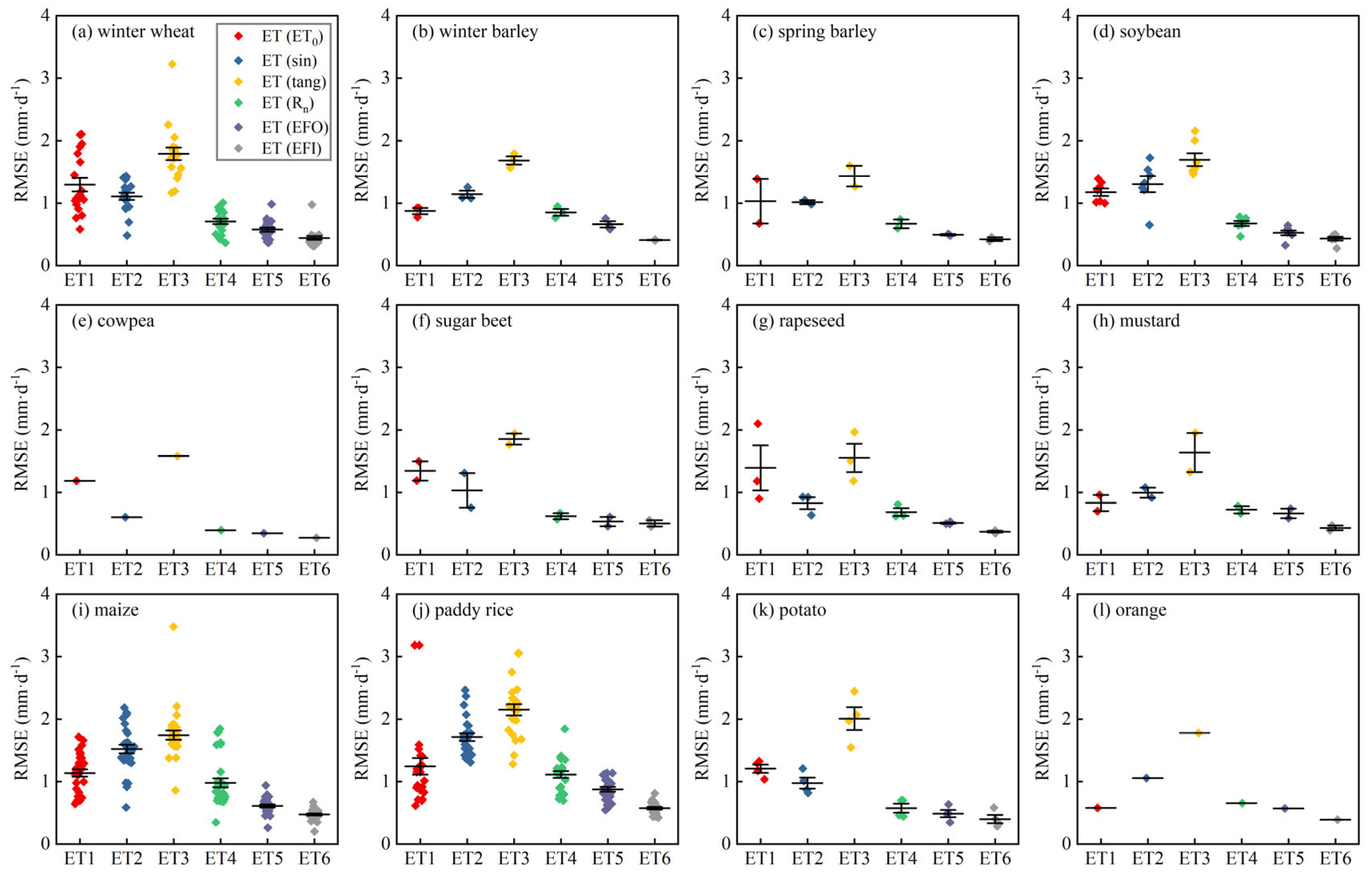
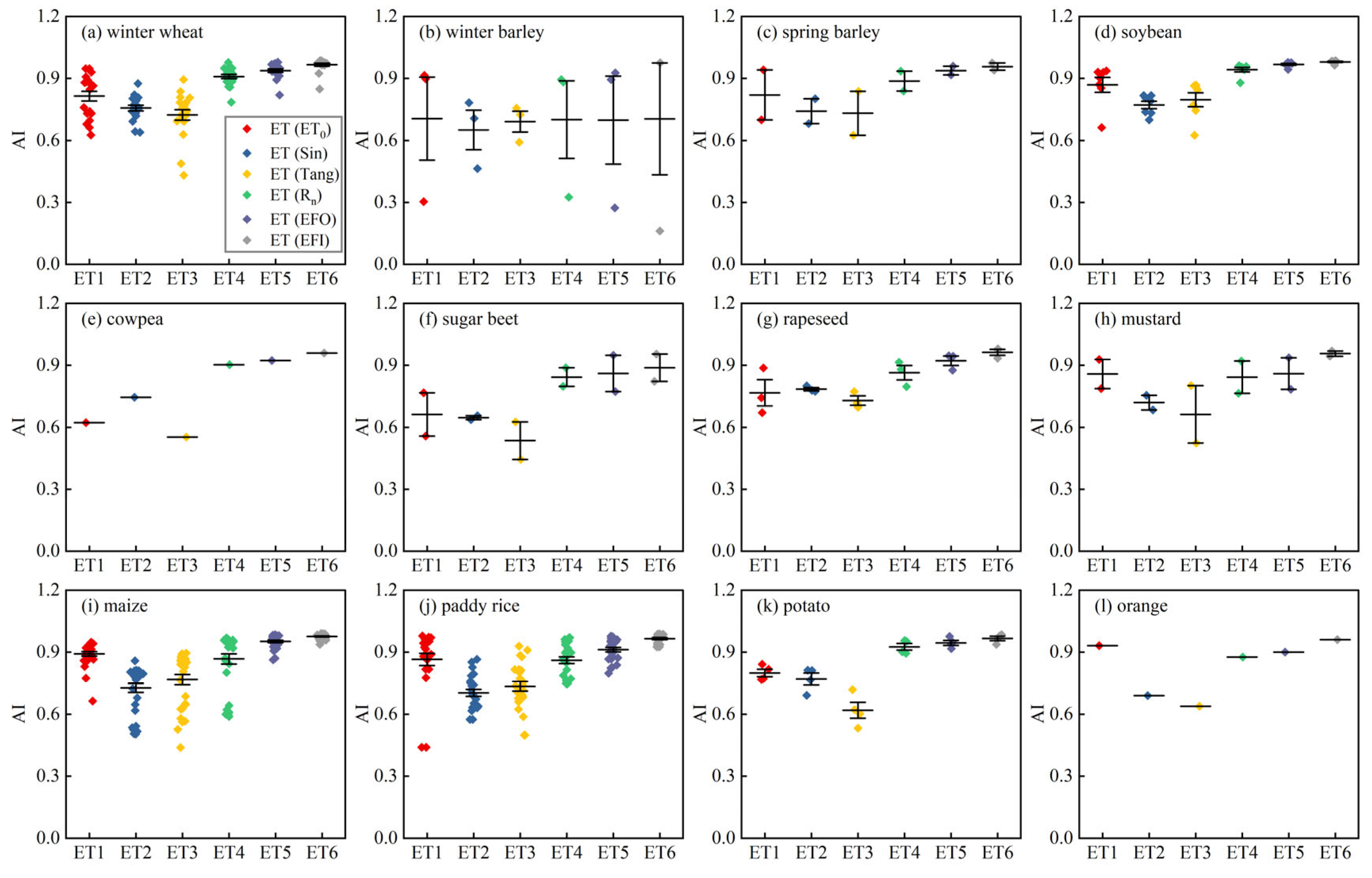
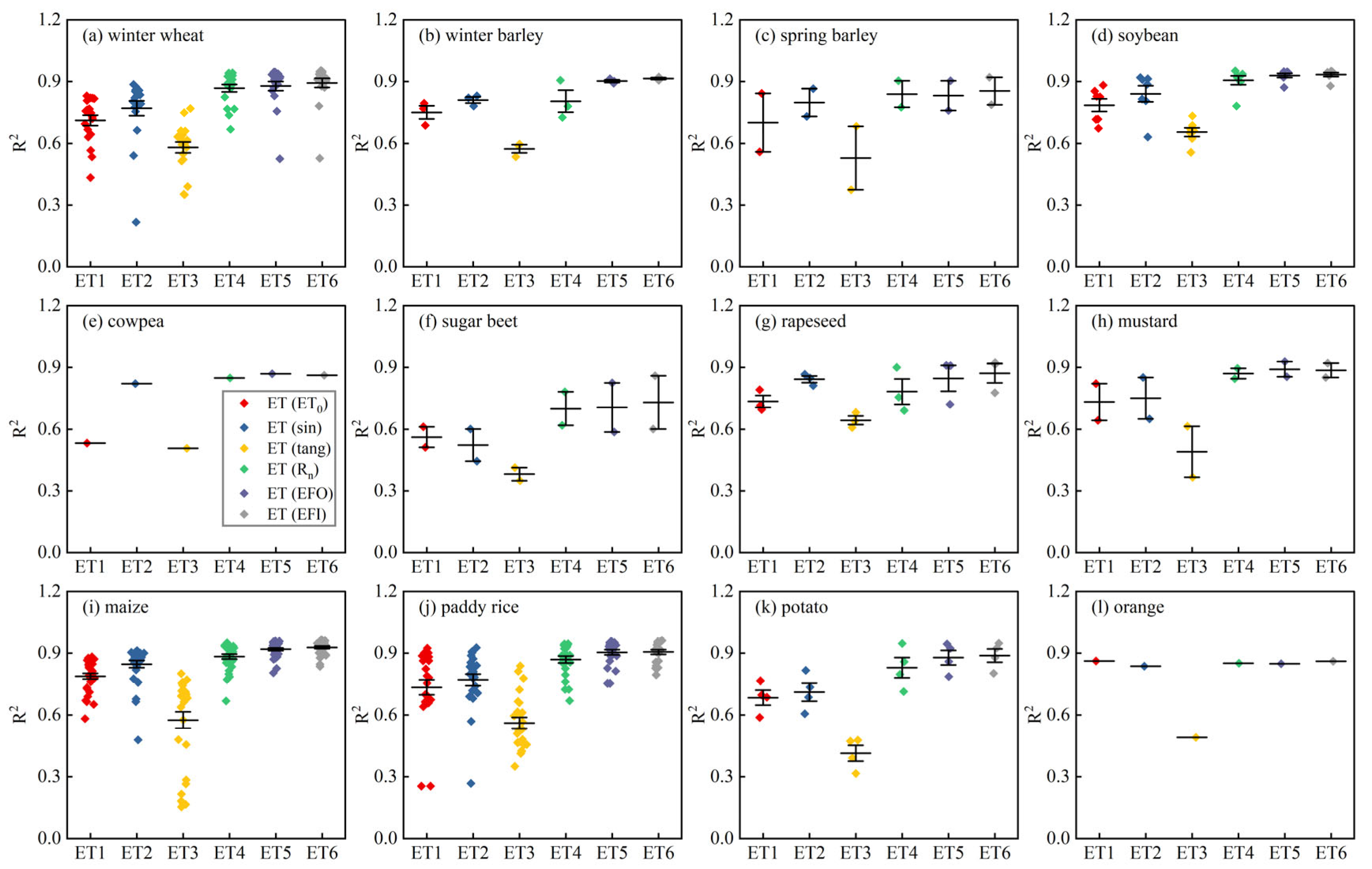
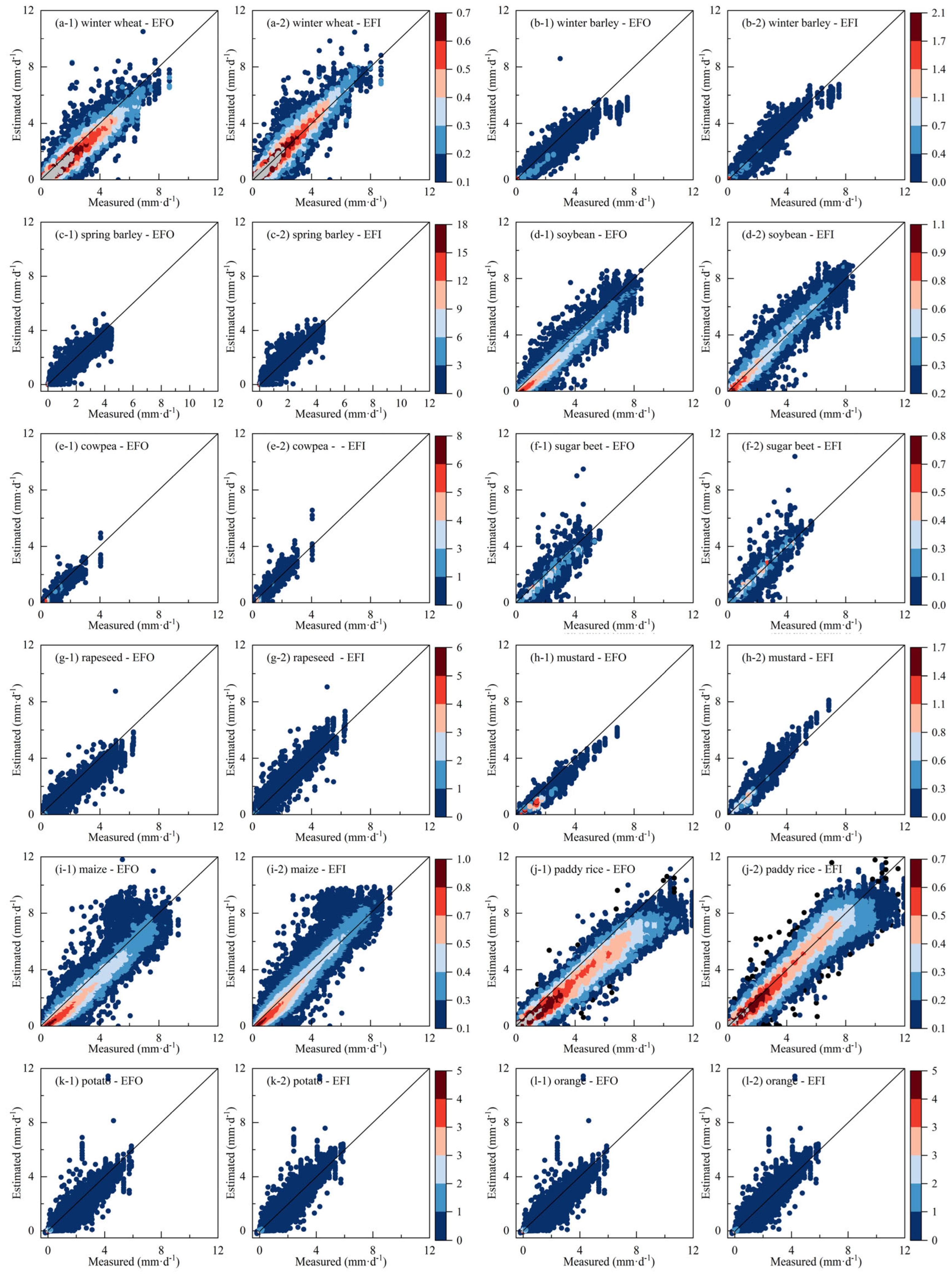
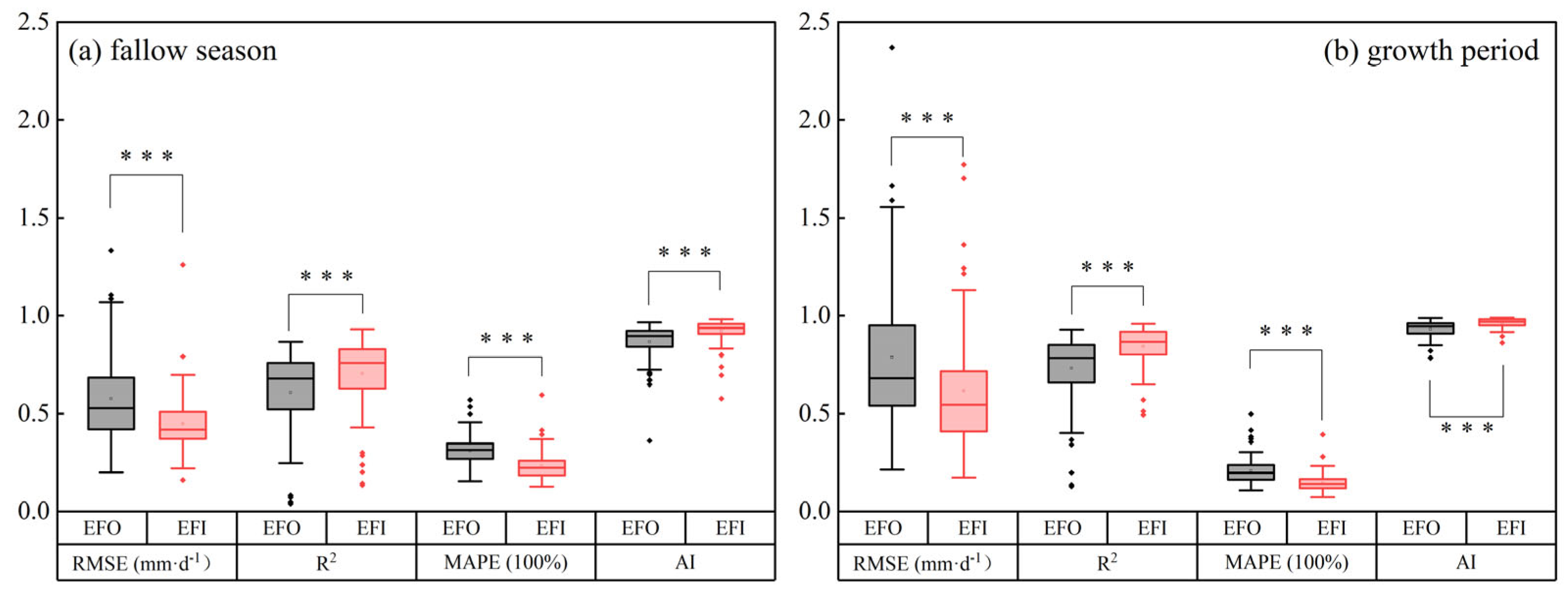
3.3. Daily ET from Daily Evaporative Fraction

The specific procedures for ETday estimation with EFI or EFO are as follows. (1) short-time EF calculation (ground-measured or SEBAL); (2) Estimating the δ and Ω; (3) EFday and ETday calculation according to Equations (12) and (13).

3.3.1. Daily ET with the EFI When Short-Time EF from Ground-Measured Data

The EFday was calculated through Equation (12) with every hourly or half-hourly EF (9:30–14:30) from EC data, and ETday was estimated by Equation (13) with the available energy (Rn-G) from the ground measurements. EFO always underestimates ETday, and EFI has somewhat corrected this bias. The improvement of ETday estimation has been particularly prominent for agricultural systems with enough data, including winter wheat, soybean, maize, and paddy rice agricultural systems (Figure 8). The four metrics also demonstrated that EFI performs better than EFO in daily ET estimation (Figure 9), with an average RMSE (0.56 mm·day−1 vs. 0.72 mm·day−1), an average MAPE (16% vs. 23%), an average AI (0.97 vs. 0.94) and an average R2 (0.88 vs. 0.79). The EFI also yielded better results during GP than FS, according to MAPE, AI, and R2, which coincides with Section 3.2. However, the conclusion is the opposite if the RMSE was used to assess EFI. The higher available energy results in a higher ET during GP, so the RMSE is higher during GP than FS. Therefore, the fact that the RMSE during GP was larger than FS did not prove that EFI is more effective during FS than during GP.

3.3.2. Daily ET from EFI When EFst from Remote Sensing Model

The SEBAL model, a remote sensing model for energy flux estimation [55], was used to estimate the instantaneous EF, upscaled to daily EF with EFI or EFO. A total of 1181 Landsat scenes from the study area over different periods were analyzed. ETday was estimated through Equation (13) with the available energy (Rn-G) from ERA5. Compared with measured data from EC systems, daily ET from EFI (solid point) is closer to the 1:1 line than from EFO (hollow point) for most agricultural systems, correcting some anomalous simulated EFst by SEBAL (Figure 10). However, EFI did not show noticeable better performance in the agricultural systems with limited data, including winter barley, spring barley, cowpea, sugar beet, rapeseed, and mustard. Unreliable results from small samples might be a reason for this [56,57]. Figure 11 reveals that EFI yielded more reliable outcomes than EFO with higher average AI (0.69 vs. 0.56), higher average R2 (0.89 vs. 0.84), lower average RMSE (1.27 mm·d−1 vs. 1.57 mm·d−1), and lower average MAPE (31% vs. 38%). The better performance of EFI demonstrated that the improved method could modify the error caused by the hypothesis of EFday equal to EFst of EFO to some extent.

4. Discussion

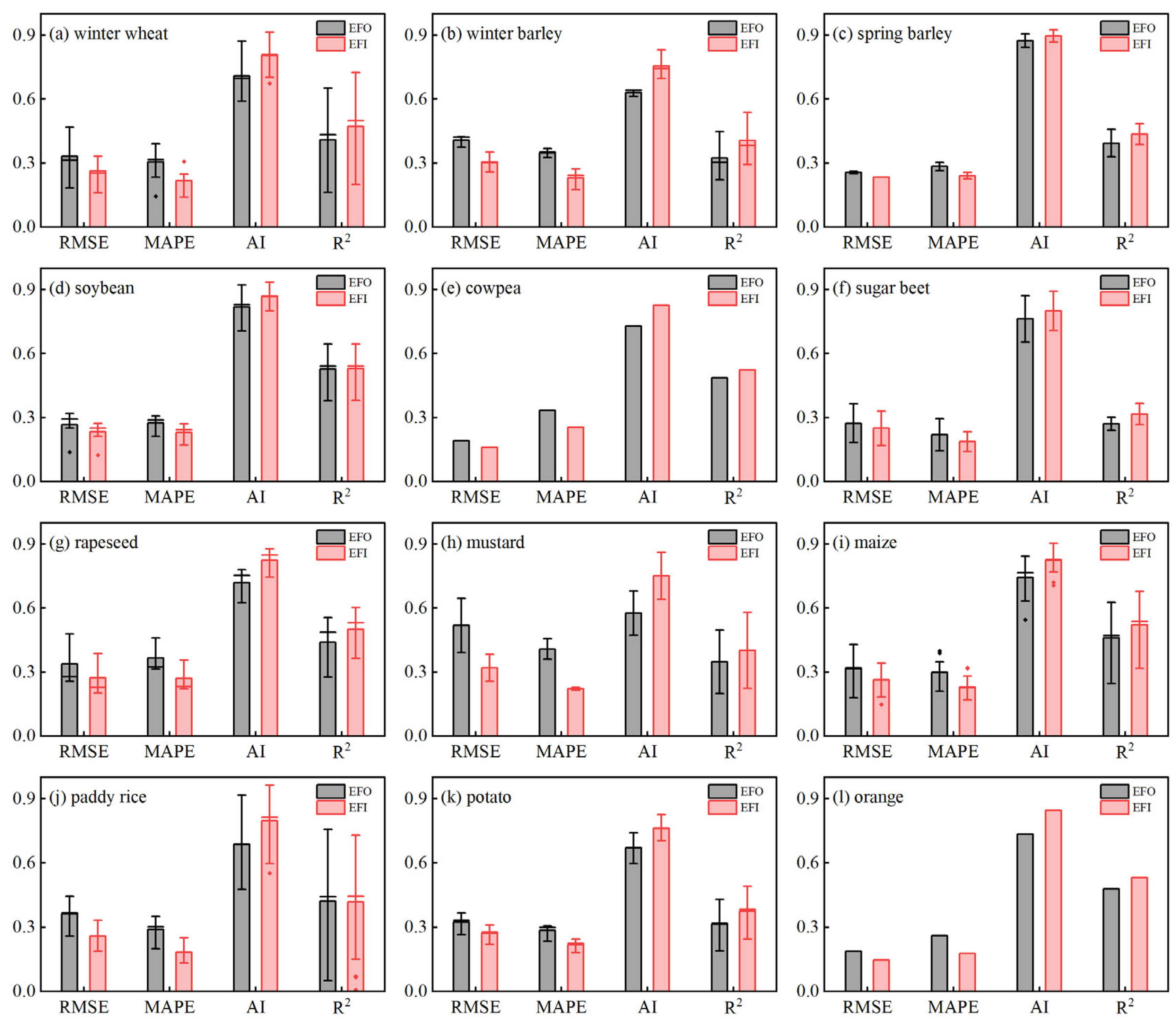
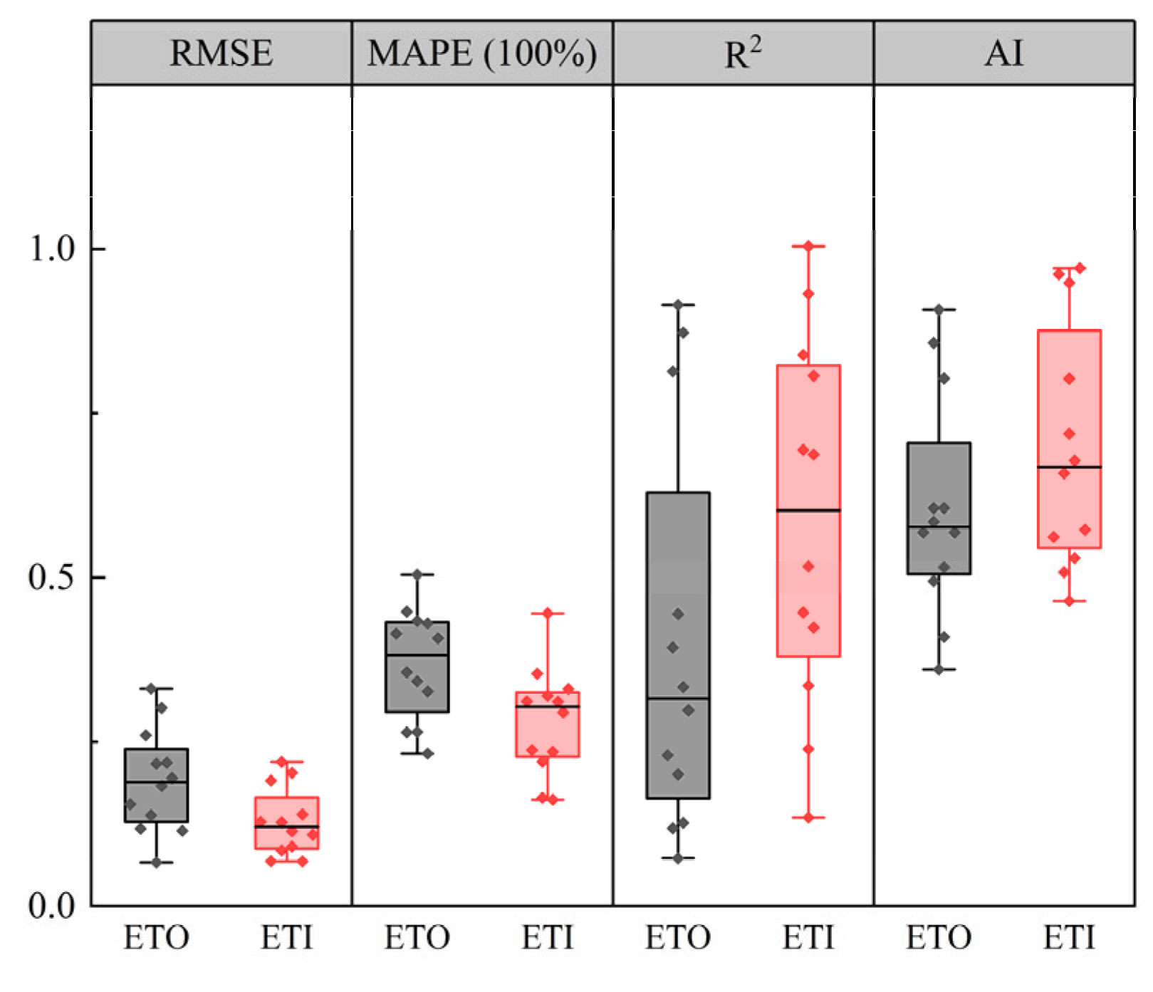
4.1. Performance of the Improved Evaporative Method

EFI can upscale the short-time EF to EFday more accurately and it performs better in ETday estimation than EFO. Most remote sensing models require VPD and Rn-G for EFst computation, and EFI typically does not require additional input. Because of this, the EFI can improve the accuracy of ETday calculation without more data entry, providing a feasible method to upscale the short-time ET to daily ET on a regional scale. According to the sources of daily Rn-G, upscaling methods, and sources of short-time EF, four cases (Table 1) were set to estimate daily ET, compared with measured daily ET from EC systems.
The performance of EFI and EFO for different cases is discrepant (Figure 12). The ETIG and ETOG are superior to ETIS and ETOS in different cases, respectively, which might result from the more significant uncertainty of estimated short-time EF by SEBAL than measured short-time EF [58]. When EFst from the EC system (Case III and Case IV), compared with EFO, EFI reduced the average MAPE from 23% to 16% and the average RMSE from 0.72 to 0.56 mm·d−1. As for short-time EF from SEBAL (Case I and Case II), the EFI also performs better than EFO, but the estimated ETday shows a more obvious difference with measured ETday than Case III and Case IV, caused by the error of short-time EF estimation. Specifically, SEBAL overestimates or underestimates the EFst for its model structure limitation in some scenarios. However, EFI does not catch these errors, resulting in the ETday estimation accuracy not improving compared with EFO for the soybean agricultural system. Nevertheless, the EFI could always improve the daily EF estimation for an accurate short-time EF (Case III and Case IV), with higher R2 and AI, lower MAPE, and RMSE. With the advancement of remote sensing technology, the EFst from remote sensing will be more and more accurate, and EFI is anticipated to deliver more valuable information for agricultural management.

4.2. Comparision with Other Upscaling Methods

Many other methods have been proposed to modify the EFO, including empirical equations [19,23,25] and theoretical derivation [24]. The moisture condition of air indexes was always contained in these methods, which was also considered in EFI. Compared with EFO, these improved methods performed better for different land covers (Table 2), such as summer corn and winter wheat croplands in the Northern China Plain (MAPE of LE from 22.8% to 11.7%), paddy fields in the Tai-Lake region of China (RMSE of ET from 0.24 mm·d−1 to 0.21 mm·d−1), and an olive orchard in central Morocco (MAPE of ET from 8% to 0.5%). For the method proposed by Hoedjes et al. [23], the measured EFst is adopted for dry conditions (Bowen ratio less than 1.5) rather than the estimated EFst. Meanwhile, the EFst is also required for wet conditions, and the 1.2, 0.00004, and 0.005 parameters might be somewhat arbitrary. So, this method is unsuitable for areas with scarce observational data. Similarly, Liu et al. [25] applied the measured daily ET to calibrate the estimated ET, generating the parameters A and B. So, the constants A and B might not be applicable for different land covers, requiring new measured data to calibrate. A result was obtained for evaporative flux ratios with Rn [59], and Liu [19] applied it to upscale the instantaneous ET. Although this method does not need the G, reduced inputs, it has a lower accuracy [19]. The G might introduce more uncertainty for ET upscaling; however, ignoring the effect of G also produces large errors in winter [60]. Compared to the first two methods, the method developed by Tang and Li [24] does not need the measured ET or EF as input and performs well. However, this method requires the ra, rs, and critical surface resistance when ET equals equilibrium ET (rs*), which is difficult to quantify precisely through remote sensing, especially for rs*. The above methods are more accurate than EFO in short-time EF upscaling, but the empirical coefficient is needed, and extra input requirements might hinder the application. So, EFI could be a choice for EFst upscale when the data are limited.
To validate the effectiveness of EFI, the five different methods were compared to EFI with EFinst from in situ measurements, including the three evaporation methods (decoupling factor method [24], net radiation method [59], and constant evaporative fraction method) and two other methods (reference evapotranspiration method [8] and sine method [7]). Specific procedures can be found in the corresponding references, and the ET from different methods were named ET(Tang), ET(Rn), ET(EFO), ET(ET0), and ET(Sine). Figure 13 shows the MAPE between measured ETday and estimated ETday from different methods, and the other index can be found in Appendix E. In general, the ETO shows the best performance for all the agricultural systems, with an average MAPE of 15.2% and a stable performance, with a standard deviation of MAPE of 0.04. EFI was developed for regional ET estimation, which is always calculated using remote sensing technology. VPD and Rn-G are needed in most ET remote sensing models, e.g., SEBS [61], METRIC [8], SEBAL [55], and RS-PM [62]. So, the EFI was used to estimate regional ET, which does not require additional input compared to the original methods.
One thing should be noticed: the error of ET(Tang) is more obvious than that of Tang and Li [24]. We carefully reviewed our data processing and calculations and found that the error associated with Tang’s method is indeed larger than EFO in certain cases. This is primarily due to the decoupling factor corresponding to the equilibrium evapotranspiration at the instantaneous scale being much larger than at the daily scale, which leads to the observed larger computed values. This phenomenon can be attributed to the differences in balance evapotranspiration between the instantaneous and daily scales, which causes larger discrepancies in the calculated decoupling factor. The climate conditions at a daily scale likely contribute to this issue, and it is possible that in the work of Tang and Li [24], they had conducted a more detailed review and validation of the base data, which could account for their more consistent results. In contrast, our analysis was based on all available data without conducting such a detailed review, which might explain the differences between our results and those reported by Tang and Li [24]. The method requires the input of rc and ra, but they did not provide detailed methods for calculating these resistances. To address this, we used the FAO-56 recommended method to estimate rc and ra, as it does not require additional data. However, it is important to note that the FAO-56 method provides only an approximation, and accurately describing these two complex parameters is challenging. This approximation could introduce additional errors into the calculation process, further contributing to the discrepancies observed in our results compared to Tang and Li [24].
It is true that any of the upscaling methods, including the ones we used in our study, could potentially provide more accurate daily ET estimates if biases were corrected through calibration against in situ measurements. Calibration is indeed an important step for improving the accuracy of any model, particularly in specific environments or conditions. However, the focus of our study was primarily on the development and evaluation of the temporal upscaling method itself rather than performing an extensive calibration of each method against in situ measurements. While calibration can undoubtedly enhance the performance of these methods, the goal here was to demonstrate the effectiveness of EFI under both calibrated and uncalibrated scenarios, as we observed good performance even with a default value of t = 0.5 (Figure 17).

4.3. The Correctness of the Hypothesis of EFI

There are two critical hypotheses for EFI: the deviation coefficient (δ) and potential deviation (Ω). The adjustment coefficient (t) and short-time EF were adopted to depict the Ω, and the optimum t for different agricultural systems was given in Section 3.2, proving the reliability of Ω. The dependability of EFI would be approved if the correctness of δ was demonstrated.
The average half-hour or hourly data (measured by EC systems) were analyzed for various agricultural systems and sites. Figure 14 illustrates a noticeable positive linear connection between η and EFst for most agricultural systems, demonstrating that the η could describe the EF intra-day when other factors were not considered to a certain extent. Besides this study, the effect of VPD [23,24] and Rn-G [16,50] on EF have been reported. As mentioned above, the results demonstrated the validity of EFI and the rationality of the hypothesis.
The relationship between η and EFst of the same crop shows a great difference in different places (Figure 14). Three crops (planted in more than four different sites) and three sites (with more than three crops) were chosen to analyze the effect factor on the relationship between η and EFst (Figure 15). The R2 between η and EFst shows large fluctuation for the same crop planting in different sites, with 0.80–0.94 for winter wheat, 0.65–0.93 for maize, and 0.74–0.99 for paddy rice. However, the R2 between η and EFst for different crops in one site shows a relatively stable state, with 0.82–0.87 for BE_Lon, 0.88–0.94 for DE_Kli, and 0.67–0.80 for US_ARM. So, the crop might not be a key factor for the relationship between η and EFst, but the circumstance factors might be (the circumstance factors would not change sharply during a short time at one location).

4.4. Uncertainty of the ETday Estimation with EFI

Compared with EFO, EFI upscaled the EFst to EFday more accurately, generating a more reliable ETday. However, some uncertainty about ETday estimation existed through EFI when the remote sensing technology was applied. Two aspects were analyzed, including sources of EFst and daily Rn (Rn,day) and the structure of EFI.

4.4.1. Uncertainty About Short-Time EF Calculation and Daily Rn

The ETday calculated from the measured EFst was more precise than calculated from the estimated EFst (SEBAL) in different sites, with an average MAPE of 16% vs. 31%, respectively. So, EFst calculation and Rn from ERA5 introduced a 15% (31% − 16%) error in ETday estimation. Nevertheless, the remote sensing approach (e.g., SEBAL) and raster climate dataset (e.g., ERA5) are crucial for regional ET calculation [63,64] at the cost of compromising calculation precision for each point.
The SEBAL, a remote sensing model suited for the homogenous underlying surface, was adopted in this study. However, uncertainties also exist in the structure [47] and some empirical coefficients [65] of SEBAL. The Rn,day and LEday errors were compared when the remote sensing image and the Rn,day measured data were available at different sites (Figure 16). LEday estimated error increased along with the Rn,day error, demonstrating that the ERA5 (source of Rn,day) would introduce the mistake when it was used to estimate ETday. On the other hand, some biases are caused by input data, including polluted pixels and coarse spatial resolution [66,67], even though the quality bands of images were applied to exclude the low-quality pixels.
While potential biases in EFst may propagate through temporal upscaling processes, this study specifically addresses temporal upscaling methodology rather than intrinsic SEBAL algorithm performance. Regarding ERA-5 reanalysis data, the meteorological variables (surface radiation, air temperature, and wind speed) have been extensively validated in prior global studies showing consistent agreement with ground observations. Given our focus on temporal scaling optimization rather than input data verification, we utilized ERA-5 datasets based on their established reliability documented in the peer-reviewed literature [17,68,69]. While we acknowledge that biases in the SEBAL model’s instantaneous ET estimations and the ERA-5 data could influence the daily ET estimations, our focus was on improving the temporal upscaling process itself. Therefore, we did not analyze the effects of other meteorological factors in the ERA5 dataset and the SEBAL model itself on ET estimates.

4.4.2. Uncertainty About the EFI Structure

It was assumed that EFday equals EFst in EFO, which ignores the heterogeneity of EF at different times. EFI considers the main circumstance factors according to P-M and P-T equations, modifying the EFO. However, some uncertainty is contained in the EFI structure.
The deviation coefficient (δ) is conducted from P-M equations in theories. However, EFI did not strictly follow Equation (4), given the model operability and data availability. Besides VPD and (Rn-G), other factors are neglected in the final modified method, which also influences the EF in some instances. According to the qualitative analysis in Section 2.3.1 and results from EFI, simplified processing is acceptable. However, further analysis should be conducted in the following studies to quantify the effects of each circumstance factor on EF.
Potential deviation (Ω) refers to the possible error between EFday and EFst, and therefore the adjustment coefficient (t) was introduced to enhance its applicability. The optimum t for the different agricultural systems was given in Section 3.2. However, for different climate conditions or circumstances, the optimum t was not analyzed, for it is challenging to quantify climate condition types and circumstances with the data of this study. EF was influenced by many factors, especially the soil water content [52,70]. Irrigation practice during GP maintained the moist soil, leading to a stable EFday. However, EFday fluctuated sharply during the FS (Figure 3) brought on by rain or other factors, leading to inaccurate potential error estimation. Future research that takes rainfall information into account might help diminish the error. To improve regional ETday estimation accuracy, the interaction of uncertainty between EFst and EFI should be explored in the future.
However, it is important to note that the purpose of this study was to develop and validate EFI at a localized scale using the available crop-specific data. While we understand that applying this method on a larger scale would require broader crop-type datasets, we believe the methodology can still provide valuable insights at the regional level where crop-type information is accessible. Moreover, when a specific value for t is not set, we assume a general value of 0.5 for all vegetation types. This approach still yields results that are superior to the original method. The specific results can be seen in Figure 17. Future research could aim to expand the applicability of this method by integrating more generalized crop classifications or by using remotely sensed data that can infer crop types at a larger scale. Additionally, efforts to create more comprehensive crop-type datasets would be beneficial for scaling up this approach.

5. Conclusions

This study developed an improved evaporative fraction method (EFI) to upscale EFst to EFday, considering saturation vapor difference and available energy without additional data requirements compared to the constant evaporative fraction method (EFO). EFI was tested for different agricultural systems, various sites, growth stages, and different sources of EFst, respectively. The optimum adjustment coefficient was given for different agricultural systems. The comparison between estimated ETday and measured ETday (from EC) demonstrates that the accuracy of EFI is superior to EFO, yielding a lower error (RMSE and MAPE) and a better consistency (AI and R2). Meanwhile, the crop might not be the main controlling factor for the relationship between η and EFst, but meteorological conditions. Since EFI requires no extra data, it is expected to be applied in converting EFst to EFday at a large scale, generating a more accurate ETday.

Author Contributions

Formal analysis, Writing-original draft, Supervision, Project administration, Visualization: J.W.; Writing-review & editing: B.L. and J.W.; Visualization: Y.L.; Methodology: Y.L. and J.W.; Validation, Y.C. and J.W.; Funding acquisition: Y.C. All authors have read and agreed to the published version of the manuscript.

Funding

The research was financially supported by the NSFC-MWR-CTGC Joint Yangtze River Water Science Research Project (No. U2040213) and Science and Technology Fundamental Resources Investigation Program (No. 2022FY101600). The authors thank the European Centre for Medium-Range Forecasts (ECMWF) for providing ERA5 reanalysis datasets at https://www.ecmwf.int/en/forecasts/datasets/ (accessed on 28 November 2024), the United States Geological Survey (USGS) for providing Landsat images and Digital Elevation Models datasets at https://www.usgs.gov/ (accessed on 28 November 2024), Fluxnet and AsiaFlux for providing flux datasets at https://fluxnet.org (accessed on 12 November 2024) and at http://asiaflux.net (accessed on 14 November 2024), the Department of Biogeochemical Integration at MPI Jena for providing at https://www.bgc-jena.mpg.de/ (accessed on 15 November 2024), and LI-COR Biosciences providing EddyPro software at https://www.licor.com (accessed on 15 November 2024).

Data Availability Statement

Dataset available on request from the authors.

Conflicts of Interest

The authors declare no conflict of interest.

Appendix A

The description of the EC datasets.
Site ID AbbreviationLatitudeLongitudeFiled AreaFetch cTime
Resolution
Crop TypeTime SpanReference
CHN_NCNC28.45°N116.01°E1.2 ha b90 mHHPR2017–2019-
US_TwtTwt38.11°N121.65°W240 ha500 mHHPR2009–2016Baldocchi et al. [71]
KR_CRKCRK38.20°N127.25°E0.4 ha b300 mHHPR2015–2018Huang et al. [72]
JP_MSEMSE36.05°N140.03°E0.5 ha b140 mHHPR2001–2006and Ono et al. [73]
IT_CasCas45.07°N8.72°E28.0 ha105 mHHPR2007–2010Meijide et al. [74]
BE_LonLon50.55°N4.74°E12.0 ha240 mHHMA SB
WW PO
2004–2014Buysse et al. [75]
DE_GebGeb51.10°N10.91°E63.8 ha*HHWW PO2001–2002Anthoni et al. [76]
DE_KliKli50.89°N13.52°E20.2 ha*HHSB RA WW
MA WBA
2005–2014Prescher et al. [77]
DE_SehSeh50.87°N6.45°E6.6 ha135 mHHWW2007–2009Schmidt et al. [78]
FR_GriGri48.84°N1.95°E20.0 ha400 mHHMU WBA2004–2009Loubet et al. [79]
IT_BCiBCi40.52°N14.96°E10.0 ha182 mHHMA2004–2010Bai et al. [80]
US_ARMARM36.60°N82.51°W12.0 ha a400 mHHWW MA
RA CO
2003–2012Raz-Yaseef et al. [81]
US_CRTCRT41.63°N96.65°W50.0 ha400 mHHSO WW2011–2013Chu et al. [82]
US_LinLin36.35°N119.09°W4.0 ha*HHOR2010Fares et al. [83]
US_Ne1Ne141.17°N83.52°W49.0 ha*HRMA2001–2012Nguy-Robertson et al. [84]
US_Ne2Ne241.16°N83.53°W52.0 ha*HRMA SO2001–2008
Note: PR: paddy rice; MA: maize; SB: sugar beet; WW: winter wheat; PO: potato; SBA: spring barley; RA: rapeseed; WBA: winter barley; SO: soybean; OR: orange; CO: cowpea; MU: mustard; HH: half-hourly time steps; HR: hourly time steps; a: the field area comes from Google Earth; b: the fields surrounded by sufficient paddy fields with same agricultural management; c: the distance from the flux tower which more than 80% of contribution to footprint; *: references do not display clearly, but demonstrate study area contribute more than 80% footprint.

Appendix B

Bowen Ratio Method

The Bowen ratio method was used to force energy balance closure. The half-hour data were used to calculate. Data with β lower than −0.7 or greater than 10 were eliminated for reliable results.
β = H o L E o
H c = β ( R n G ) 1 + β
L E c = R n G H c
where subscript o and c are the original and corrected data, respectively; EBR is the energy balance ratio.

Appendix C

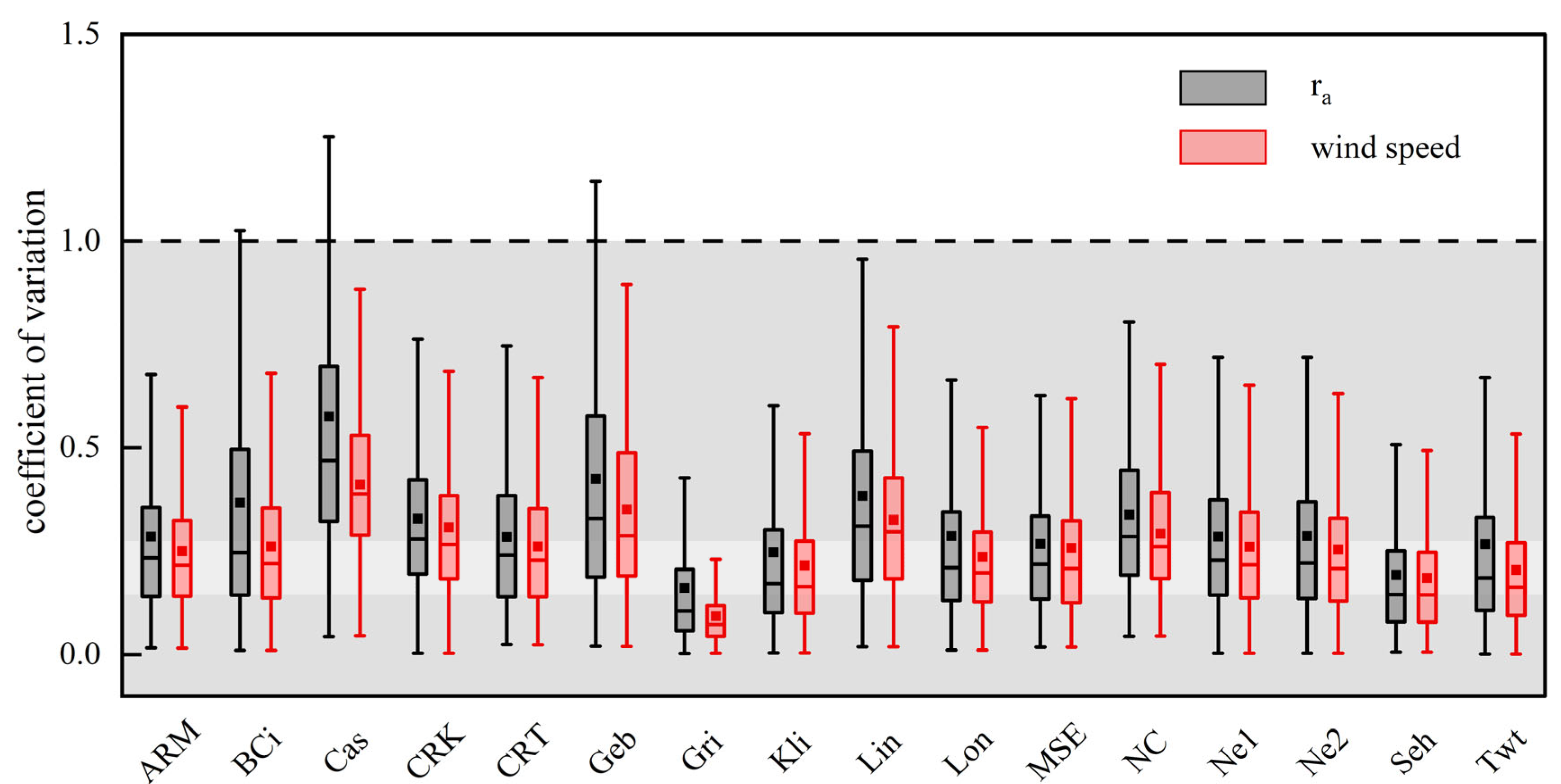
The Variation in Daytime Wind Speed and ra

The coefficient of variation (CV) of daytime wind speed and ra were analyzed for 16 sites (Figure A1).
C V = σ μ
where σ is the standard deviation; μ is the mean value. The CV value between 0 and 0.1 represents weak variation and that of 0.1–1 represents moderate variation [84].
Figure A1. The coefficient of wind speed and aerodynamic resistance in 16 different sites. The gray area represents the moderate variation range.
Remotesensing 17 01016 g0a1
The results show that the variation of ra is somewhat greater than wind speed, but both are in moderate variation. Over 99% of days, the CV of the wind speed is less than 1, with an average CV of 0.23. Also, Over 97% of days, the CV of the ra is less than 1, with an average CV of 0.26, which is close to the threshold of weak variation. Malek et al. [40] and Obisesan and Jegede [84] also demonstrated that the range of ra variation is limited from 9:30 to 14:30 in one day. So, the variation in ra introduced by wind speed is not great in the 16 sites and is not taken into account in this study.

Appendix D

SEBAL model description and computation algorithm.

Appendix D.1. Latent Heat Flux (LE)

The Surface Energy Balance Algorithm for Land (SEBAL) is a single-source energy balance model calculating latent heat flux through the residual energy principle. All the parameters are instantaneous as shown in Appendix B. The study area was delineated to encompass the entire Landsat image covering the research site, a strategic selection that both ensures the inclusion of hot end-member and preserves methodological repeatability for future applications.
L E = R n G H
where LE is the latent heat flux, W·m−2; Rn is the surface net radiation, W·m−2; H is the sensible heat flux, W·m−2; and G is the soil heat flux, W·m−2.

Appendix D.2. Net Radiation (Rn)

The hourly net radiation is derived from ERA5, and daily Rn is obtained through hourly data accumulating.

Appendix D.3. Soil Heat Flux (G)

Soil heat flux (G) is the exchange of heat flux in shallow soil, calculated through a semi-empirical equation.
G = ( 0.0038 + 0.0074 α 0 ) ( 1 0.978 N D V I 4 ) R n T s
α 0 = θ i ρ i 0.0018 α path τ sw 2
τ s w = 0.38 + 0.627 exp 0.00146 P K t cos θ hor 0.075 W cos θ hor
W = 0.14 e a P + 2.1
N D V I = ( θ nir θ r ) / ( θ nir + θ r )
where Ts is the land surface temperature from Landsat images, K; NDVI is the normalized difference vegetation index; α0 is surface albedo, dimensionless; θi is the dimensionless surface reflectance of band i from Landsat images; ρi is the dimensionless weight coefficient of band i; αpath is the dimensionless path radiation coefficient; τsw is broad-band atmospheric transmissivity; P is the atmospheric pressure, kPa; Kt is the turbidity coefficient; θhor is solar zenith angle over a horizontal surface; W is water in the atmosphere, mm; θnir and θr are the surface reflectance of the near-infrared and red band from Landsat images.

Appendix D.4. Sensible Heat Flux (H)

Sensible heat flux can be obtained according to the temperature gradient of surface and near-surface air.
H = ρ a c p d T r ah
where ρa is the air density, kg·m−3; cp is the air-specific heat at constant pressure, J·kg−1·K−1; dT is the near-surface temperature difference between 2.0 m (z2) and 0.1 m (z1), K; and rah is the aerodynamic resistance, s·m−1.
r ah = ln ( z 2 / z 1 ) k u f
where k is von Karman’s constant, 0.41, and uf is the friction velocity, m·s−1.
d T = a T s , datum + b
T s , datum = T s 0.0065 Z
where a and b are the determined constants for a given satellite image, dimensionless, which are estimated through the cold and hot end-member; Ts,datum is surface temperature adjusted to a common elevation data for each image pixel using the elevation data (Z, m) from DEM dataset. The cold end-member is located at well-vegetated fields or water bodies, where H is assumed to be 0. The hot end-member means the arid conditions, where the LE is set to 0. A simplified calibration using the inverse modeling at extreme conditions algorithm was used to determine the cold/hot member and the detailed process can be referred to [17].
d T hot = ( R n G ) hot r ah ,   hot ρ a ,   hot c p
d T cold = 0
a = d T hot d T cold T s , hot T s , cold = d T hot T s , hot T s , cold
b = T s , cold d T hot d T cold T s , hot T s , hot T s , cold = T s , cold d T hot T s , hot T s , cold
where the subscript hot and cold represent the hot and cold pixels, respectively.
The above calculation should be conducted under a stable atmosphere condition, so the Obukhov stability length (L) was used to examine the atmosphere condition and calibrate until H becomes stable.
L = ρ a C p u f 3 T s k g H
where g is gravitational acceleration, 9.8 m·s−1.
The corrected value for uf can be calculated as follows.
u f = k u 200 ln ( 200 / z om ) ψ m   ( 200 )
where u200 is the wind speed at a blending height assumed to be 200 m, m·s−1; zom is momentum roughness length, m; Ψm(200) is stability correction for momentum transport at 200 m.
r ah = ln ( z 2 / z 1 ) ψ h   ( z 2 ) + ψ h   ( z 1 ) k u f
where Ψh(z1) and Ψh(z2) are stability corrections for heat transport at z1 and z2 heights, respectively.
When L < 0 (unstable conditions),
ψ m   ( 200 ) = 2 ln ( 1 + x 200 2 ) + ln ( 1 + x 200 2 2 ) 2 arctan ( x 200 ) + 0.5 π
ψ h   ( 2 ) = 2 ln ( 1 + x 2 2 )
ψ h   ( 1 ) = 2 ln ( 1 + x 0.1 2 )
x h = ( 1 16 h L ) 0.25
where h represents 0.1 m, 2 m, and 200 m, respectively.
When L = 0 (neutral conditions), L = 0, Ψh = 0 and Ψm = 0.
When L > 0 (stable conditions),
ψ m   ( 200 ) = 5 ( 2 L )
ψ h   ( 2 ) = 5 ( 2 L )
ψ h   ( 0 . 1 ) = 5 ( 0.1 L )

Appendix D.5. Evaporation Fraction

The instantaneous evaporative fraction (EF) can be read as follows.
E F = L E R n G

Appendix E

The figures of different indexes about different short-time ET upscaling methods.
The core concepts of the first four methods are fundamentally similar, as they all assume that a specific physical quantity remains constant throughout the day. The decoupling factor method assumes that the decoupling factor remains unchanged over the course of the day. The net radiation method assumes that the ratio of ETst to net radiation stays constant throughout the day. EFO assumes that the ratio of instantaneous ET to available energy remains constant during the day. The reference evapotranspiration method assumes that the ratio of instantaneous ET to reference crop evapotranspiration remains unchanged throughout the day. In contrast, the sine method assumes that the variation in evapotranspiration over the day follows a sinusoidal pattern. Decoupling factors and EF methods are physically sound and net radiation and ETo methods are data-efficient, while the sine method offers simplicity.
Figure A2. RMSE between measured ETday and estimated ETday from different methods. The ET(ETO), ET(sin), ET(tang), ET(Rn), ET(EFO), and ET(EFI) represent the ETday is derived from the reference evapotranspiration method, sine method, decoupling factor method, net radiation method, EFO, and EFI, respectively.
Remotesensing 17 01016 g0a2
Figure A3. AI between measured ETday and estimated ETday from different methods.
Remotesensing 17 01016 g0a3
Figure A4. R2 between measured ETday and estimated ETday from different methods.
Remotesensing 17 01016 g0a4

Appendix F

List of principal symbols and acronyms
AcronymMeaningUnit
ECEddy covariance-
EFEvaporative fraction: the ratio between latent heat flux and available energy-
EFdayDaily evaporative fraction-
EFIImproved evaporative fraction method-
EFOConstant evaporative fraction method-
EFstShort-time evaporative fraction-
ERA5European Centre for Medium-Range Weather Forecasts Reanalysis v5, a raster climate dataset-
ETEvapotranspirationMm·d−1
ETdayDaily evapotranspirationmm·d−1
ETIGETday estimated with EFI when EFst and daily Rn-G come from SEBAL and ERA5, respectivelymm·d−1
ETISETday estimated with EFI when EFst and daily Rn-G come from EC system and ground-measured data, respectivelymm·d−1
ETOGETday estimated with EFO when EFst and daily Rn-G come from SEBAL and ERA5, respectivelymm·d−1
ETOSETday estimated with EFO when EFst and daily Rn-G come from EC system and ground-measured data, respectivelymm·d−1
ETstShort-time evapotranspirationmm·d−1
FSFallow season-
GSoil heat fluxW·m−2
GPGrowth period-
HSensible heat fluxW·m−2
LELatent heat fluxW·m−2
RnNet heat radiationW·m−2
SEBALA Surface Energy Balance Algorithm for Land model used to estimate energy flux-
tAdjustment coefficient of Ω-
VPDVapor pressure deficitkPa
δDeviation coefficient between EFst and EFday-
ηRatio between VPD and available energykPa·W−1·m2
τAvailable energyW·m−2
ΩPotential deviation between EFst and EFday-

References

  1. Jackson, R.D.; Reginato, R.J.; Idso, S.B. Wheat canopy temperature: A practical tool for evaluating water requirements. Water Resour. Res. 1977, 13, 651–656. [Google Scholar] [CrossRef]
  2. Price, J.C. Estimation of Regional Scale Evapotranspiration Through Analysis of Satellite Thermal-infrared Data. IEEE Trans. Geosci. Remote Sens. 1982, GE-20, 286–292. [Google Scholar] [CrossRef]
  3. Price, J.C. The potential of remotely sensed thermal infrared data to infer surface soil moisture and evaporation. Water Resour. Res. 1980, 16, 787–795. [Google Scholar] [CrossRef]
  4. Seguin, B.; Itier, B. Using midday surface temperature to estimate daily evaporation from satellite thermal IR data. Int. J. Remote Sens. 1983, 4, 371–383. [Google Scholar] [CrossRef]
  5. Carlson, T.N.; Capehart, W.J.; Gillies, R.R. A new look at the simplified method for remote sensing of daily evapotranspiration. Remote Sens. Environ. 1995, 54, 161–167. [Google Scholar] [CrossRef]
  6. Sugita, M.; Brutsaert, W. Daily evaporation over a region from lower boundary layer profiles measured with radiosondes. Water Resour. Res. 1991, 27, 747–752. [Google Scholar] [CrossRef]
  7. Jackson, R.D.; Hatfield, J.L.; Reginato, R.J.; Idso, S.B.; Pinter, P.J. Estimation of daily evapotranspiration from one time-of-day measurements. Agr. Water Manag. 1983, 7, 351–362. [Google Scholar] [CrossRef]
  8. Allen, R.G.; Tasumi, M.; Trezza, R. Satellite-Based Energy Balance for Mapping Evapotranspiration with Internalized Calibration (METRIC)—Model. J. Irrig. Drain Eng. 2007, 133, 380–394. [Google Scholar] [CrossRef]
  9. Tasumi, M.; Allen, R.G.; Trezza, R.; Wright, J.L. Satellite-Based Energy Balance to Assess Within-Population Variance of Crop Coefficient Curves. J. Irrig. Drain Eng. 2005, 29, 94–109. [Google Scholar] [CrossRef]
  10. Liu, G.; Liu, Y.; Xu, D. Comparison of evapotranspiration temporal scaling methods based on lysimeter measurements. J. Remote Sens. 2011, 15, 270–280. [Google Scholar] [CrossRef]
  11. Shuttleworth, W.J.; Gurney, R.J.; Hsu, A.Y.; Ormsby, J.P. FIFE: The Variation in ENERGY partition at Surface at Surfacae Flux Sites; IAHS Publisher: Wallingford, UK, 1989. [Google Scholar]
  12. Gomez, M.; Olioso, A.; Sobrino, J.; Jacob, F. Retrieval of evapotranspiration over the Alpilles/ReSeDA experimental site using airborne POLDER sensor and a thermal camera. Remote Sens. Environ. 2005, 96, 399–408. [Google Scholar] [CrossRef]
  13. Li, F.; Xin, X.; Peng, Z.; Liu, Q. Estimating daily evapotranspiration based on a model of evaporative fraction (EF) for mixed pixels. Hydrol. Earth Syst. Sci. 2019, 23, 949–969. [Google Scholar] [CrossRef]
  14. Lian, X.; Piao, S.; Huntingford, C.; Li, Y.; Zeng, Z.; Wang, X.; Ciais, P.; McVicar, T.R.; Peng, S.; Ottlé, C.; et al. Partitioning global land evapotranspiration using CMIP5 models constrained by observations. Nat. Clim. Change 2018, 8, 640–646. [Google Scholar] [CrossRef]
  15. Sobrino, J.A.; Gómez, M.; Jiménez-Muñoz, J.C.; Olioso, A. Application of a simple algorithm to estimate daily evapotranspiration from NOAA–AVHRR images for the Iberian Peninsula. Remote Sens. Environ. 2007, 110, 139–148. [Google Scholar] [CrossRef]
  16. Zhang, L.; Lemeur, R. Evaluation of daily evapotranspiration estimates from instantaneous measurements. Agr. Forest. Meteorol. 1995, 74, 139–154. [Google Scholar] [CrossRef]
  17. Laipelt, L.; Henrique Bloedow Kayser, R.; Santos Fleischmann, A.; Ruhoff, A.; Bastiaanssen, W.; Erickson, T.A.; Melton, F. Long-term monitoring of evapotranspiration using the SEBAL algorithm and Google Earth Engine cloud computing. ISPRS. J. Photogramm. 2021, 178, 81–96. [Google Scholar] [CrossRef]
  18. Peng, J.; Borsche, M.; Liu, Y.; Loew, A. How representative are instantaneous evaporative fraction measurements of daytime fluxes? Hydrol. Earth Syst. Sci. 2013, 17, 3913–3919. [Google Scholar] [CrossRef]
  19. Liu, Z. The accuracy of temporal upscaling of instantaneous evapotranspiration to daily values with seven upscaling methods. Hydrol. Earth Syst. Sci. 2021, 25, 4417–4433. [Google Scholar] [CrossRef]
  20. Van Niel, T.G.; McVicar, T.R.; Roderick, M.L.; van Dijk, A.I.; Beringer, J.; Hutley, L.B.; van Gorsel, E. Upscaling latent heat flux for thermal remote sensing studies: Comparison of alternative approaches and correction of bias. J. Hydrol. 2012, 468–469, 35–46. [Google Scholar] [CrossRef]
  21. Xu, T.; Liu, S.; Xu, L.; Chen, Y.; Jia, Z.; Xu, Z.; Nielson, J. Temporal Upscaling and Reconstruction of Thermal Remotely Sensed Instantaneous Evapotranspiration. Remote Sens. 2015, 7, 3400–3425. [Google Scholar] [CrossRef]
  22. Nichols, W.E.; Cuenca, R.H. Evaluation of the evaporative fraction for parameterization of the surface energy balance. Water Resour. Res. 1993, 29, 3681–3690. [Google Scholar] [CrossRef]
  23. Hoedjes, J.; Chehbouni, A.; Jacob, F.; Ezzahar, J.; Boulet, G. Deriving daily evapotranspiration from remotely sensed instantaneous evaporative fraction over olive orchard in semi-arid Morocco. J. Hydrol. 2008, 354, 53–64. [Google Scholar] [CrossRef]
  24. Tang, R.; Li, Z. An improved constant evaporative fraction method for estimating daily evapotranspiration from remotely sensed instantaneous observations. Geophys. Res. Lett. 2017, 44, 2319–2326. [Google Scholar] [CrossRef]
  25. Liu, X.; Xu, J.; Zhou, X.; Wang, W.; Yang, S. Evaporative fraction and its application in estimating daily evapotranspiration of water-saving irrigated rice field. J. Hydrol. 2020, 584, 124317. [Google Scholar] [CrossRef]
  26. Suleiman, A.; Crago, R. Hourly and Daytime Evapotranspiration from Grassland Using Radiometric Surface Temperatures. Agron. J. 2004, 96, 384–390. [Google Scholar] [CrossRef]
  27. Wei, J.; Cui, Y.; Luo, Y. Rice growth period detection and paddy field evapotranspiration estimation based on an improved SEBAL model: Considering the applicable conditions of the advection equation. Agr. Water Manag. 2023, 278, 108141. [Google Scholar] [CrossRef]
  28. Amani, S.; Shafizadeh-Moghadam, H. A review of machine learning models and influential factors for estimating evapotranspiration using remote sensing and ground-based data. Agr. Water Manag. 2023, 284, 108324. [Google Scholar] [CrossRef]
  29. Blatchford, M.L.; Mannaerts, C.M.; Zeng, Y.; Nouri, H.; Karimi, P. Status of accuracy in remotely sensed and in-situ agricultural water productivity estimates: A review. Remote Sens. Environ. 2019, 234, 111413. [Google Scholar] [CrossRef]
  30. Wei, J.; Cui, Y.; Luo, W.; Luo, Y. Mapping Paddy Rice Distribution and Cropping Intensity in China from 2014 to 2019 with Landsat Images, Effective Flood Signals, and Google Earth Engine. Remote Sens. 2022, 14, 759. [Google Scholar] [CrossRef]
  31. Hollinger, D.Y.; Goltz, S.M.; Davidson, E.A.; Lee, J.T.; Tu, K.; Valentine, H.T. Seasonal patterns and environmental control of carbon dioxide and water vapour exchange in an ecotonal boreal forest. Glob. Change Biol. 1999, 5, 891–902. [Google Scholar] [CrossRef]
  32. Wilson, K.; Goldstein, A.; Falge, E.; Aubinet, M.; Baldocchi, D.; Berbigier, P.; Bernhofer, C.; Ceulemans, R.; Dolman, H.; Field, C.; et al. Energy balance closure at FLUXNET sites. Agr. Forest. Meteorol. 2002, 113, 223–243. [Google Scholar] [CrossRef]
  33. Twine, T.E.; Kustas, W.P.; Norman, J.M.; Cook, D.R.; Houser, P.R.; Meyers, T.P.; Prueger, J.H.; Starks, P.J.; Wesely, M.L. Correcting eddy-covariance flux underestimates over a grassland. Agr. Forest. Meteorol. 2000, 103, 279–300. [Google Scholar] [CrossRef]
  34. Allen, R.G.; Pereira, L.S.; Raes, D.; Smith, M. Crop Evapotranspiration: Guidelines for Computing Crop Water Requirements; FAO: Rome, Italy, 1998; ISBN 9251042195. [Google Scholar]
  35. Yan, H.; Zhang, C.; Coenders Gerrits, M.; Acquah, S.J.; Zhang, H.; Wu, H.; Zhao, B.; Huang, S.; Fu, H. Parametrization of aerodynamic and canopy resistances for modeling evapotranspiration of greenhouse cucumber. Agr. Forest. Meteorol. 2018, 262, 370–378. [Google Scholar] [CrossRef]
  36. Rana, G.; Katerji, N.; Mastrorilli, M.; El Moujabber, M. Evapotranspiration and canopy resistance of grass in a Mediterranean region. Theor Appl Climatol 1994, 50, 61–71. [Google Scholar] [CrossRef]
  37. Rouphael, Y.; Colla, G. Modelling the transpiration of a greenhouse zucchini crop grown under a Mediterranean climate using the Penman-Monteith equation and its simplified version. Aust. J. Agric. Res. 2004, 55, 931. [Google Scholar] [CrossRef]
  38. Bailey, B.J.; Montero, J.I.; Biel, C.; Wilkinson, D.J.; Anton, A.; Jolliet, O. Transpiration of Ficus benjamina: Comparison of measurements with predictions of the Penman-Monteith model and a simplified version. Agr. Forest. Meteorol. 1993, 65, 229–243. [Google Scholar] [CrossRef]
  39. Montero, J.I.; Antón, A.; Muñoz, P.; Lorenzo, P. Transpiration from geranium grown under high temperatures and low humidities in greenhouses. Agr. Forest. Meteorol. 2001, 107, 323–332. [Google Scholar] [CrossRef]
  40. Malek, E.; Bingham, G.E.; McCurdy, G.D. Continuous measurement of aerodynamic and alfalfa canopy resistances using the Bowen ratio-energy balance and Penman-Monteith methods. Bound. Lay. Meteorol. 1992, 59, 187–194. [Google Scholar] [CrossRef]
  41. Rana, G.; Ferrara, R.M.; Cona, F.; de Lorenzi, F. Actual transpiration and canopy resistance in a Mediterranean vineyard irrigated with saline water. Irrig. Sci. 2021, 39, 469–481. [Google Scholar] [CrossRef]
  42. Bailey, W.G.; Davies, J.A. The effect of uncertainty in aerodynamic resistance on evaporation estimates from the combination model. Bound. Lay. Meteorol. 1981, 20, 187–199. [Google Scholar] [CrossRef]
  43. Li, S.; Wang, G.; Sun, S.; Fiifi Tawia Hagan, D.; Chen, T.; Dolman, H.; Liu, Y. Long-term changes in evapotranspiration over China and attribution to climatic drivers during 1980–2010. J. Hydrol. 2021, 595, 126037. [Google Scholar] [CrossRef]
  44. Li, S.; Wang, G.; Zhu, C.; Lu, J.; Ullah, W.; Hagan, D.F.T.; Kattel, G.; Peng, J. Attribution of global evapotranspiration trends based on the Budyko framework. Hydrol. Earth Syst. Sci. 2022, 26, 3691–3707. [Google Scholar] [CrossRef]
  45. Yao, Y.; Liao, X.; Xiao, J.; He, Q.; Shi, W. The sensitivity of maize evapotranspiration to vapor pressure deficit and soil moisture with lagged effects under extreme drought in Southwest China. Agr. Water Manag. 2023, 277, 108101. [Google Scholar] [CrossRef]
  46. Cheng, M.; Shi, L.; Jiao, X.; Nie, C.; Liu, S.; Yu, X.; Bai, Y.; Liu, Y.; Liu, Y.; Song, N.; et al. Up-scaling the latent heat flux from instantaneous to daily-scale: A comparison of three methods. J. Hydrol. Reg. Stud. 2022, 40, 101057. [Google Scholar] [CrossRef]
  47. Cheng, M.; Jiao, X.; Li, B.; Yu, X.; Shao, M.; Jin, X. Long time series of daily evapotranspiration in China based on the SEBAL model and multisource images and validation. Earth Syst. Sci. Data 2021, 13, 3995–4017. [Google Scholar] [CrossRef]
  48. Willmott, C.J.; Ackleson, S.G.; Davis, R.E.; Feddema, J.J.; Klink, K.M.; Legates, D.R.; O’Donnell, J.; Rowe, C.M. Statistics for the evaluation and comparison of models. J. Geophys. Res. 1985, 90, 8995. [Google Scholar] [CrossRef]
  49. Li, S.; Kang, S.; Li, F.; Zhang, L.; Zhang, B. Vineyard evaporative fraction based on eddy covariance in an arid desert region of Northwest China. Agr. Water Manag. 2008, 95, 937–948. [Google Scholar] [CrossRef]
  50. Reichstein, M.; Falge, E.; Baldocchi, D.; Papale, D.; Aubinet, M.; Berbigier, P.; Bernhofer, C.; Buchmann, N.; Gilmanov, T.; Granier, A.; et al. On the separation of net ecosystem exchange into assimilation and ecosystem respiration: Review and improved algorithm. Glob. Change Biol. 2005, 11, 1424–1439. [Google Scholar] [CrossRef]
  51. Farah, H.O.; Bastiaanssen, W.; Feddes, R.A. Evaluation of the temporal variability of the evaporative fraction in a tropical watershed. Int. J. Appl. Earth Obs. 2004, 5, 129–140. [Google Scholar] [CrossRef]
  52. Pérez-Delgado, M.-L.; Günen, M.A. A comparative study of evolutionary computation and swarm-based methods applied to color quantization. Expert Syst. Appl. 2023, 231, 120666. [Google Scholar] [CrossRef]
  53. Kalma, J.D.; McVicar, T.R.; McCabe, M.F. Estimating Land Surface Evaporation: A Review of Methods Using Remotely Sensed Surface Temperature Data. Surv. Geophys. 2008, 29, 421–469. [Google Scholar] [CrossRef]
  54. Bastiaanssen, W.; Menenti, M.; Feddes, R.A.; Holtslag, A. A remote sensing surface energy balance algorithm for land (SEBAL). 1. Formulation. J. Hydrol. 1998, 212–213, 198–212. [Google Scholar] [CrossRef]
  55. Charter, R.A. Study samples are too small to produce sufficiently precise reliability coefficients. J. Gen. Psychol. 2003, 130, 117–129. [Google Scholar] [CrossRef]
  56. Colaizzi, P.D.; Evett, S.R.; Howell, T.A.; Tolk, J.A. Comparison of Five Models to Scale Daily Evapotranspiration from One-Time-of-Day Measurements. Trans. ASABE 2006, 49, 1409–1417. [Google Scholar] [CrossRef]
  57. Brutsaert, W.; Sugita, M. Application of self-preservation in the diurnal evolution of the surface energy budget to determine daily evaporation. J. Geophys. Res. Atmos. 1992, 97, 18377–18382. [Google Scholar] [CrossRef]
  58. Cammalleri, C.; Anderson, M.C.; Kustas, W.P. Upscaling of evapotranspiration fluxes from instantaneous to daytime scales for thermal remote sensing applications. Hydrol. Earth Syst. Sci. 2014, 18, 1885–1894. [Google Scholar] [CrossRef]
  59. Su, Z. The Surface Energy Balance System (SEBS) for estimation of turbulent heat fluxes. Hydrol. Earth Syst. Sci. 2002, 6, 85–100. [Google Scholar] [CrossRef]
  60. Mu, Q.; Zhao, M.; Running, S.W. Improvements to a MODIS global terrestrial evapotranspiration algorithm. Remote Sens. Environ. 2011, 115, 1781–1800. [Google Scholar] [CrossRef]
  61. Li, X.; Long, D.; Han, Z.; Scanlon, B.R.; Sun, Z.; Han, P.; Hou, A. Evapotranspiration Estimation for Tibetan Plateau Headwaters Using Conjoint Terrestrial and Atmospheric Water Balances and Multisource Remote Sensing. Water Resour. Res. 2019, 55, 8608–8630. [Google Scholar] [CrossRef]
  62. Herman, M.R.; Nejadhashemi, A.P.; Abouali, M.; Hernandez-Suarez, J.S.; Daneshvar, F.; Zhang, Z.; Anderson, M.C.; Sadeghi, A.M.; Hain, C.R.; Sharifi, A. Evaluating the role of evapotranspiration remote sensing data in improving hydrological modeling predictability. J. Hydrol. 2018, 556, 39–49. [Google Scholar] [CrossRef]
  63. Shamloo, N.; Taghi Sattari, M.; Apaydin, H.; Valizadeh Kamran, K.; Prasad, R. Evapotranspiration estimation using SEBAL algorithm integrated with remote sensing and experimental methods. Int. J. Digit. Earth 2021, 14, 1638–1658. [Google Scholar] [CrossRef]
  64. Kiptala, J.K.; Mohamed, Y.; Mul, M.L.; van der Zaag, P. Mapping evapotranspiration trends using MODIS and SEBAL model in a data scarce and heterogeneous landscape in Eastern Africa. Water Resour. Res. 2013, 49, 8495–8510. [Google Scholar] [CrossRef]
  65. Ochege, F.U.; Luo, G.; Obeta, M.C.; Owusu, G.; Duulatov, E.; Cao, L.; Nsengiyumva, J.B. Mapping evapotranspiration variability over a complex oasis-desert ecosystem based on automated calibration of Landsat 7 ETM+ data in SEBAL. GISci. Remote Sens. 2019, 49, 1305–1332. [Google Scholar] [CrossRef]
  66. Jaafar, H.H.; Sujud, L.H. High-resolution satellite imagery reveals a recent accelerating rate of increase in land evapotranspiration. Remote Sens. Environ. 2024, 315, 114489. [Google Scholar] [CrossRef]
  67. Ippolito, M.; de Caro, D.; Cannarozzo, M.; Provenzano, G.; Ciraolo, G. Evaluation of daily crop reference evapotranspiration and sensitivity analysis of FAO Penman-Monteith equation using ERA5-Land reanalysis database in Sicily, Italy. Agr. Water Manag. 2024, 295, 108732. [Google Scholar] [CrossRef]
  68. Yang, C.; Ma, Y.; Yuan, Y. Terrestrial and Atmospheric Controls on Surface Energy Partitioning and Evaporative Fraction Regimes Over the Tibetan Plateau in the Growing Season. JGR Atmos. 2021, 126, e2021JD035011. [Google Scholar] [CrossRef]
  69. Baldocchi, D.; Knox, S.; Dronova, I.; Verfaillie, J.; Oikawa, P.; Sturtevant, C.; Matthes, J.H.; Detto, M. The impact of expanding flooded land area on the annual evaporation of rice. Agr. For. Meteorol. 2016, 223, 181–193. [Google Scholar] [CrossRef]
  70. Huang, Y.; Ryu, Y.; Jiang, C.; Kimm, H.; Kim, S.; Kang, M.; Shim, K. BESS-Rice: A remote sensing derived and biophysical process-based rice productivity simulation model. Agr. For. Meteorol. 2018, 256–257, 253–269. [Google Scholar] [CrossRef]
  71. Ono, K.; Maruyama, A.; Kuwagata, T.; Mano, M.; Takimoto, T.; Hayashi, K.; Hasegawa, T.; Miyata, A. Canopy-scale relationships between stomatal conductance and photosynthesis in irrigated rice. Glob. Change Biol. 2013, 19, 2209–2220. [Google Scholar] [CrossRef]
  72. Meijide, A.; Manca, G.; Goded, I.; Magliulo, V.; Di Tommasi, P.; Seufert, G.; Cescatti, A. Seasonal trends and environmental controls of methane emissions in a rice paddy field in Northern Italy. Biogeosciences 2011, 8, 3809–3821. [Google Scholar] [CrossRef]
  73. Buysse, P.; Bodson, B.; Debacq, A.; de Ligne, A.; Heinesch, B.; Manise, T.; Moureaux, C.; Aubinet, M. Carbon budget measurement over 12 years at a crop production site in the silty-loam region in Belgium. Agr. For. Meteorol. 2017, 246, 241–255. [Google Scholar] [CrossRef]
  74. Anthoni, P.M.; Knohl, A.; Rebmann, C.; Freibauer, A.; Mund, M.; Ziegler, W.; Kolle, O.; Schulze, E.-D. Forest and agricultural land-use-dependent CO2 exchange in Thuringia, Germany. Glob. Change Biol. 2004, 10, 2005–2019. [Google Scholar] [CrossRef]
  75. Prescher, A.-K.; Grünwald, T.; Bernhofer, C. Land use regulates carbon budgets in eastern Germany: From NEE to NBP. Agr. For. Meteorol. 2010, 150, 1016–1025. [Google Scholar] [CrossRef]
  76. Schmidt, M.; Reichenau, T.G.; Fiener, P.; Schneider, K. The carbon budget of a winter wheat field: An eddy covariance analysis of seasonal and inter-annual variability. Agr. For. Meteorol. 2012, 165, 114–126. [Google Scholar] [CrossRef]
  77. Loubet, B.; Laville, P.; Lehuger, S.; Larmanou, E.; Fléchard, C.; Mascher, N.; Genermont, S.; Roche, R.; Ferrara, R.M.; Stella, P.; et al. Carbon, nitrogen and Greenhouse gases budgets over a four years crop rotation in northern France. Plant Soil 2011, 343, 109–137. [Google Scholar] [CrossRef]
  78. Bai, Y.; Zhang, J.; Zhang, S.; Yao, F.; Magliulo, V. A remote sensing-based two-leaf canopy conductance model: Global optimization and applications in modeling gross primary productivity and evapotranspiration of crops. Remote Sens. Environ. 2018, 215, 411–437. [Google Scholar] [CrossRef]
  79. Raz-Yaseef, N.; Billesbach, D.P.; Fischer, M.L.; Biraud, S.C.; Gunter, S.A.; Bradford, J.A.; Torn, M.S. Vulnerability of crops and native grasses to summer drying in the U.S. Southern Great Plains. Agric. Ecosyst. Environ. 2015, 213, 209–218. [Google Scholar] [CrossRef]
  80. Chu, H.; Chen, J.; Gottgens, J.F.; Ouyang, Z.; John, R.; Czajkowski, K.; Becker, R. Net ecosystem methane and carbon dioxide exchanges in a Lake Erie coastal marsh and a nearby cropland. J. Geophys. Res. Biogeosci. 2014, 119, 722–740. [Google Scholar] [CrossRef]
  81. Fares, S.; Weber, R.; Park, J.-H.; Gentner, D.; Karlik, J.; Goldstein, A.H. Ozone deposition to an orange orchard: Partitioning between stomatal and non-stomatal sinks. Environ. Pollut. 2012, 169, 258–266. [Google Scholar] [CrossRef]
  82. Nguy-Robertson, A.; Suyker, A.; Xiao, X. Modeling gross primary production of maize and soybean croplands using light quality, temperature, water stress, and phenology. Agr. For. Meteorol. 2015, 213, 160–172. [Google Scholar] [CrossRef]
  83. Obisesan, O.E.; Jegede, O.O. Evaluation of selected parameterizations of aerodynamic resistance to heat transfer for the estimation of sensible heat flux at a tropical site in Ile-Ife, Nigeria. Ife J. Sci. 2022, 24, 95–108. [Google Scholar]
  84. Allen, R.G.; Burnett, B.; Kramber, W.; Huntington, J.; Kjaersgaard, J.; Kilic, A.; Kelly, C.; Trezza, R. Automated Calibration of the METRIC—Landsat Evapotranspiration Process. JAWRA J. Am. Water Resour. Assoc. 2013, 49, 563–576. [Google Scholar] [CrossRef]
Figure 1. The distribution of the EC systems that are adopted in this study and the map of the experiment field.
Remotesensing 17 01016 g001
Figure 2. Workflow of improved evaporative fraction method (EFI). EF1, ET1, EF2, and ET2 are different EF or ET when EFst and Rn-G from various sources (EF1, ET1: EFst from the EC system and (Rn-G)day from a ground-measured system; EF2, ET2: EFst from the remote sensing model and (Rn-G)day from raster climate variables dataset) which were used to assess the EFI. δ is the deviation coefficient between daily EF and short-time EF. Ω is the potential deviation between daily EF and short-time EF. Landsat is the satellite image. DEM is the digital elevation model dataset. ERA5 is the raster climate variables dataset. SEBAL is a remote sensing model which is used to estimate evapotranspiration.
Remotesensing 17 01016 g002
Figure 3. The average diurnal variation in EF for different agricultural systems. The abscissa 9:00 represents the average value of the period 8:30–9:00. The Gri site is continuously rotating, so mustard fields have a very short fallow season, and the fallow season is not shown in subgraph (h). The orange tree is a perennial plant, so the fallow season of the orange orchard is not shown in subgraph (l).
Remotesensing 17 01016 g003
Figure 4. The mean absolute percentage error (MAPE) variation between measured daily EF and upscaled EF from EFI for different agricultural systems, with different t values. The dashed line represents the MAPE between measured daily EF and upscaled EF from EFO.
Remotesensing 17 01016 g004
Figure 5. Assessment of EFI and EFO (estimated EF) for different agricultural systems. RMSE: root mean square error; MAPE: mean relative error; AI: agreement index; R2: determination coefficient.
Remotesensing 17 01016 g005
Figure 6. Performance EFO and EFI in EFday estimation when EFst from SEBAL for different crops. Each point represents one type of crop.
Remotesensing 17 01016 g006
Figure 7. The performance (estimated EF) of EFI and EFO during the fallow season and growth periods. *** represents the metric of EFI which does significantly tend to be greater or smaller than that of EFO at the 0.0001 level through the Wilcoxon signed ranks test.
Remotesensing 17 01016 g007
Figure 8. Measured versus EFO or EFI estimated daily ET for different agricultural systems. The color scale represents the values of the kernel density estimate, with larger values indicating denser data points.
Remotesensing 17 01016 g008
Figure 9. The performance (estimated ET) of EFI and EFO during the fallow season and growth periods. *** represents the metric of EFI which does significantly tend to be greater or smaller than that of EFO at the 0.0001 level through the Wilcoxon signed ranks test.
Remotesensing 17 01016 g009
Figure 10. Comparison of EC measured daily ET and estimated ETday for EFI (solid point) and EFO (hollow point) in different sites (when EFst from SEBAL).
Remotesensing 17 01016 g010
Figure 11. Performance EFO and EFI in ETday estimation when EFst from SEBAL for different crops. Each point represents one type of crop.
Remotesensing 17 01016 g011
Figure 12. The assessment of EFI and EFO when short-time EF comes from measured or SEBAL in different sites. The estimated daily ET was compared to the daily ET from the EC system in 16 sites. ETOS is the daily ET computed with EFO when short-time EF and daily Rn-G come from SEBAL and ERA5, respectively. ETIS is the daily ET computed with EFI when short-time EF and daily Rn-G come from SEBAL and ERA5, respectively. ETOS is the daily ET computed with EFO when short-time EF and daily Rn-G come from the EC system and ground-measured data, respectively. ETIS is the daily ET computed with EFI when short-time EF and daily Rn-G come from the EC system and ground-measured data, respectively.
Remotesensing 17 01016 g012
Figure 13. MAPE between measured ETday and estimated ETday from different methods. One point represents a year of data.
Remotesensing 17 01016 g013
Figure 14. The scatterplot of η and EFst for different agricultural systems. ARM(7) means the seven years of data at the ARM site were adopted.
Remotesensing 17 01016 g014
Figure 15. The R2 between η and EFst in different agricultural systems (a) and sites (b).
Remotesensing 17 01016 g015
Figure 16. Comparison between the Rn,day error (difference between ERA5 and ground-measured Rn,day) and LE error (difference between estimated and ground-measured LE). N represents the number of dots in each gridding.
Remotesensing 17 01016 g016
Figure 17. The MAPE for winter wheat ETday estimation with EFO and EFI (t = 0.5 and optimum t).
Remotesensing 17 01016 g017
Table 1. Brief description of different cases of daily ET estimation.
CaseETday SymbolUpscaling MethodsSources of Daily Rn-GSources Short-Time EF
Case ⅠETOSEFOERA5SEBAL
Case ⅡETISEFIERA5SEBAL
Case ⅢETOGEFOGround-measuredEC system
Case ⅣETIGEFIGround-measuredEC system
Table 2. The information about different improved evaporation methods. Subscript “mea” means measured data; subscript “est” means estimated data; subscript “st” means short-time data; subscript “day” means daily data from 0:00 to 23:59; Rs is solar radiation; RH is the relative humidity; EF is the evaporation fraction; β is the Bowen Ratio; VPD is vapor pressure deficit of the air; A and B are the fitting parameters from measured data and estimated data; Rn is net radiation; G is soil heat flux; Ta is air temperature; ra is aerodynamic resistance; rs is surface resistance; r* is critical surface resistance when ET equals equilibrium ET; Ω* is the decoupling factor when ET equals equilibrium ET.
ProvidersAssumptionsInputsCore EquationsAccuracy Improvement Compared to EFO
Hoedjes et al. [23]The linear relationship between Rs, RH and EF; the scaling factor was the ratio of EFmea,st and EFest,st.Rs, RH, and EFmea,st E F day = E F mea , st β > 1.5 1.2 ( 0.0004 R s , day + 0.005 R H day ) E F mea , st E F est , st β 1.5 MAPE: 8% vs. 0.5%
Liu et al. [25]VPD controls the simulated error between estimated ETday with EFO and measured ETday.A, B, and VPD E T EF , day = E F st ( R n G ) day E T day = A E T EF , day + B V P D day RMSE: 0.24 vs. 0.21 mm·d−1
Liu [19]The ratio of LE to Rn is a constant.EFst L E s t R n , s t = L E d a y R d a y MAPE 20% vs. 18%
Tang and Li [24]The decoupling factor is constant for one day.Ta, ra, rs, and r * E T day = E F est , st ( R n G ) day Δ day Δ day + γ Δ st + γ Δ st Ω st * Ω day * MAPE: 22.8% vs. 11.7%
Note: PR: paddy rice; MA: maize; SB: sugar beet; WW: winter wheat; PO: potato; SBA: spring barley; RA: rapeseed; WBA: winter barley; SO: soybean; OR: orange; CO: cowpea; MU: mustard; HH: half-hourly time steps; HR: hourly time steps; a: the field area comes from Google Earth; b: the fields surrounded by sufficient paddy fields with same agricultural management; c: the distance from the flux tower which more than 80% of contribution to footprint; *: references do not display clearly, but demonstrate study area contribute more than 80% footprint.
Disclaimer/Publisher’s Note: The statements, opinions and data contained in all publications are solely those of the individual author(s) and contributor(s) and not of MDPI and/or the editor(s). MDPI and/or the editor(s) disclaim responsibility for any injury to people or property resulting from any ideas, methods, instructions or products referred to in the content.

