Abstract
This paper presents the technical design of the pathfinder Barcelona Raman LIDAR (pBRL) for the northern site of the Cherenkov Telescope Array Observatory (CTAO-N) located at the Roque de los Muchachos Observatory (ORM). The pBRL is developed for continuous atmospheric characterization, essential for correcting high-energy gamma-ray observations captured by Imaging Atmospheric Cherenkov Telescopes (IACTs). The LIDAR consists of a steerable telescope with a 1.8 m parabolic mirror and a pulsed Nd:YAG laser with frequency doubling and tripling. It emits at wavelengths of 355 nm and 532 nm to measure aerosol scattering and extinction through two elastic and Raman channels. Built upon a former Cherenkov Light Ultraviolet Experiment (CLUE) telescope, the pBRL’s design includes a Newtonian mirror configuration, a coaxial laser beam, a near-range system, a liquid light guide and a custom-made polychromator. During a one-year test at the ORM, the stability of the LIDAR and semi-remote-controlled operations were tested. This pathfinder leads the way to designing a final version of a CTAO Raman LIDAR which will provide real-time atmospheric monitoring and, as such, ensure the necessary accuracy of scientific data collected by the CTAO-N telescope array.
Keywords:
Raman LIDAR; design; aerosols; atmospheric effects; gamma-ray astrophysics; IACTs; polychromator; Liquid Light Guide; Licel; PMT 1. Introduction
The Cherenkov Telescope Array Observatory (CTAO) [1,2] is the next generation observatory of ground-based Imaging Atmospheric Cherenkov Telescopes (IACTs). The CTAO will observe high-energy cosmic photons for high-energy astrophysics research; the widely used term ’gamma rays’ will be used from now on throughout this article. The observatory is composed of more than 70 telescopes at two locations: in the northern hemisphere, CTAO-N is found at the Observatorio del Roque de Los Muchachos (ORM, La Palma, Canary Islands, Spain, 28° N 17° W), and in the southern hemisphere, CTAO-S will be constructed at a site belonging to the European Southern Observatory (ESO, Cerro Paranal, Chile, 24° S 70° W). The telescope arrays are spread over an area of approximately one square kilometre and are located at altitudes of around 2200 m above sea level.
IACTs indirectly detect cosmic gamma rays with energies ranging from tens of GeV to several tens of TeV (1 GeV = 109 electronvolt (eV), 1 TeV = 1012 eV). At these energies, gamma rays interact with atmospheric nuclei disintegrating into extended atmospheric showers (EAS) of elementary particles (see Figure 1). With a very-high-energy (VHE) photon interaction length of about 47.1 g/cm2 in air [3], for vertical incidence, at a pressure level of 32 mbar (corresponding to ∼23 km a.s.l.), half of the impacting gamma rays have converted to an electron–positron pair that produces the particle shower. The length of an EAS depends on the primary energy of the gamma ray on average, so that higher-energy showers penetrate deeper into the atmosphere than lower-energy ones (see Figure 1). Furthermore, the penetration depth depends on the incidence direction of the original gamma ray, and hence the particle shower. Charged particles within the EAS are ultra-relativistic during most of the shower development and emit Cherenkov radiation [4]. That radiation is observed on the ground as a brief burst (few nanoseconds) of mainly UV (300–400 nm) light, which illuminates an area of 105–106 m2. Most of the observed Cherenkov light originates from altitudes of 5–17 km a.s.l. (for vertical incidence) and from 8–18 km a.s.l. (for low elevation angles of observation) [4,5].
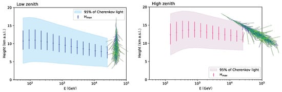
Figure 1.
Ranges of shower development as a function of gamma-ray energy; left for vertical incidence, right for shower inclined by 60° with respect to the zenith (30° elevation). The points show the mean location of the shower maximum, and lines the ranges within which 95% of the showers exhibit the maximum. The bands show the range within which 95% of the observable Cherenkov light is emitted. The data used to produce this figure have been adopted from [5,6]. On the right side, a simulated particle shower of 300 GeV energy is shown (image adopted from [7]). Green lines denote photons and blue lines electrons and positrons.
The development of an EAS is affected by the refractive index of air (modulated by the density profile of the atmosphere) [8,9], whereas propagation of Cherenkov light to ground is strongly influenced by atmospheric extinction: molecular and aerosol scattering, as well as scattering by clouds [5,10,11] and by aerosols in the lower stratosphere (15–20 km a.s.l.), as a consequence of, for example, strong stratovolcanic eruptions [12] or large-scale vertical advection [13].
The dominant contribution to the systematic uncertainty in the energy and flux reconstruction of IACTs results from an inaccurate determination of the atmospheric transmittance of Cherenkov light [14,15]. For this reason, CTAO has chosen [16] to continuously monitor and assess the aerosol extinction profile along the line of sight of the observing telescopes [17], together with the monitoring of the aerosol optical depth (AOD) across the observed field of view [18]. For the first part, specifically designed Raman LIDARs (RLs) have been proposed [17,19]. The RLs are supposed to point approximately in the direction of the CTAO science target and therefore need to be designed to be fully orientable within a cone from zenith to 20° elevation.Astronomical target tracking is not necessary if the duration of data collection is within seconds to a few minutes. RL operation should not interfere with data taking or even the operation of other close-by astronomical installations [20,21].
In recent years, several astroparticle experiments that use the atmosphere as part of their detector have committed themselves to use LIDARs [22,23,24,25]. In particular, the MAGIC Collaboration has developed a custom-fit elastic LIDAR as well as a dedicated algorithm for IACT data correction using aerosol extinction information [5,11]. Although that LIDAR has been absolutely calibrated, achieving correlated calibration-period-wise accuracies of the vertical aerosol optical depth (VAOD) of the ground layer better than ±0.01 (uncorrelated ones of ∼±0.015) [26], Schmuckermaier et al. [5] have also shown the limitations of an elastic system based on only one wavelength. Elastic LIDAR systems without absolute calibration reach accuracies of only 20% for extinction profiles, even with the help of auxiliary sun photometer data that provide estimates of the LIDAR ratio [27,28].
Given the nature of the observed Cherenkov light, LIDARs at IACT installations shall characterize the entire troposphere and the lower stratosphere, i.e., reach at least 20 km height a.s.l. or ∼45 km range for elevation angles of 25° and an observatory altitude of ∼2 km a.s.l. Modern astronomical sites are characterized by extremely clear skies [29], no clouds or only a few clouds [30] and low dust content [31] or few episodes of dust intrusions [32]. Moreover, very bad atmospheric conditions lead to abandoning scientific operations and hence do not require atmosphere characterization. IACT science data cannot be reasonably analysed with AODs larger than about 0.7, even if the optical properties of the atmosphere are well characterized [5]. The heights of the nocturnal planetary boundary layer (PBL) at these sites normally reach below 800 m above ground [11,33] and their fine structure need not be resolved [34] for gamma-ray energies below about 1 TeV, because Cherenkov light is emitted entirely above it [4]. Above these energies, gamma-ray showers penetrate down to the ground, and part of the Cherenkov light is emitted within the nocturnal boundary layer; nevertheless, such Cherenkov light is not observable for the CTAO telescopes if the shower impacts at distances larger than 100 m from the telescopes [35]. Therefore, aerosol profiling for CTAO is acceptable with a range resolution below a few hundred meters, as long as the absolute AOD of the ground layer is determined with accuracies better than 0.03. This can already be achieved with elastic lines only if decent efforts are made to continuously maintain absolute LIDAR calibration [11,26]. Finally, optically thick and low (cumulus) clouds are of no interest for precise characterization, since observations will be aborted anyhow under such conditions. Only optically thin clouds, and possibly optically thick clouds at high altitudes [35], require detailed monitoring. Given the large longitudinal extension of the Cherenkov light-emitting particle showers, clouds above a geometrical thickness of 4 km need to be characterized according to their measured profile [36]. Below that value, a standard average profile might be used. Note that Fruck et al. [11] have shown that an elastic LIDAR can already determine the optical depth of such clouds with sufficient accuracy; hence, Raman capabilities are strictly required only up to the end of the PBL.
RLs designed to reach the stratosphere and even the lower mesosphere using pulsed Nd:YAG lasers and receiver telescopes of ∼1 m diameter class have been used for a few decades already [24,37,38,39,40,41], although recently, significant advances have been made using order-of-magnitude more powerful excimer lasers [42]. These systems rely on static LIDARs, so, the design of pointable LIDARs means an additional challenge.
In this report, we discuss an RL pathfinder for CTAO-N. The instrument is dubbed pBRL (pathfinder Barcelona Raman LIDAR). The pBRL is designed, maintained and operated by the Institut de Física d’Altes Energies (IFAE, Barcelona, Spain) and the Universitat Autonòma de Barcelona (UAB, Barcelona, Spain) in collaboration with the University of Nova Gorica (Slovenia), the University of Padova and the Istituto Nazionale di Fisica Nucleare (INFN, sez. Padova, Italy). It has been designed for a 4-channel (2 elastic, 2 Raman) orientable RL, composed of a 1.8 m parabolic mirror, with , with a Newtonian alt-az mount and a 532 nm frequency-doubled and 355 nm frequency-tripled Nd:YAG pulsed laser.
Atmospheric LIDARs [43,44] often use Nd:YAG lasers with their 1064 nm wavelength and the second and third harmonic at 532 nm and 355 nm, respectively. In particular, the fundamental line provides stronger backscattering signals from coarse aerosols compared to the molecular background. For our purpose, however, 1064 nm lies rather far from the typical Cherenkov light emission band and may cause interference with the optical telescopes at the ORM observing in the I and J bands. Finally, strong illumination of the Liquid Light Guide (LLG) by infrared light may cause faster degradation of it. Therefore, our choice fell on the 355 nm and the 532 nm lines, both found well within the wavelength range of the observed Cherenkov light spectrum [45]. In addition to that, a Raman channel allows one to discriminate relatively well between aerosols of different LIDAR ratios and achieve accuracies well below 10% for aerosol extinction coefficients [46], as required for CTAO science data analysis (see Section 2). A natural choice is the relatively strong vibrational–rotational Raman (VRR) Stokes lines of 355 nm scattering on N2 [47] centred at 387 nm. Adding a second Raman channel at 607 nm (the VRR Stokes line of 532 nm) allows us to retrieve the Ångström extinction exponent with the required precision. Note that the Raman backscatter cross-section for 532 nm is only about 20% that at 355 nm [47,48,49]. The inclusion of further lines, like CO2, water vapour, additional elastic and Raman channels, is not strictly needed for the purpose of CTAO and was discarded.
The pBRL structure has been built on a recycled Cherenkov Light Ultraviolet Experiment (CLUE) telescope enclosed in a 20 ft standard maritime container [50], already equipped with a large parabolic reflector of 1.8 m diameter. CLUE was a gamma-ray detector array installed at the ORM, sensitive to the UV light from Cherenkov showers in the range 190–230 nm [51]. The array was dismantled in 2002, but some of the individual containers still exist with the telescope inside. The pBRL group acquired two CLUE containers for the purpose of building LIDARs. A third container was purchased by the Laboratoire Univers et Particules de Montpellier (LUPM), France, which also renovated it as an RL for CTAO-S [52]. At the moment of writing this document, only one of the two Barcelona containers has been refurbished and has become a pathfinder Raman LIDAR for CTAO.
This paper is structured as follows. In Section 2, we introduce the requirements the instruments have to satisfy to be used for the purpose of CTAO. In Section 3, we detail the current technical solutions adopted for the refurbishment of the CLUE container to build the pBRL. In Section 4, we calibrate the LIDAR performance. In Section 5, we discuss the way pBRL is operated within the CTAO framework. We summarize and conclude in Section 6.
2. Technical Requirements
This section collects the technical requirements that an RL shall meet in accordance with the CTAO guidelines. CTAO has defined a set of level B product requirements (Level A product requirements are those that apply to the product as a whole, i.e., the CTAO observatory, whereas level B products requirements apply to its different systems), separated into scientific and performance requirements, operation and survival conditions for the two array sites, and finally reliability and availability requirements.
2.1. Scientific and Performance Requirements
Energy scale and flux scale. CTAO requires an accuracy, both on the energy of reconstructed gamma-ray photons and the reconstructed gamma-ray flux of <10% at 90% confidence level, at energies between 50 GeV and 300 TeV. Several processes contribute to these systematic uncertainties, among which their are limitations in the understanding of the telescopes and their degradation with time, and the precise state of the atmosphere. The latter is allowed to contribute to the uncertainty of the energy scale by <8% and consists of several individual contributions related to the accurate modelling of the development of air showers, the molecular density and refractive index profile and the light-absorbing molecules. Further uncertainties include limitations in the knowledge of the extinction of Cherenkov light through scattering processes with molecules, clouds and dust layers. Clouds and dust layers are allowed to contribute the largest uncertainty, about <3% each, for the Cherenkov light yield on the ground. A similar breakdown leads to a requirement of <5% for the estimated contribution of aerosols to the systematic uncertainty of the reconstruction of gamma-ray fluxes.
Wavelengths. The CTAO telescopes are sensitive to Cherenkov light in the wavelength range from 300 nm to ∼700 nm. The Cherenkov light spectrum falls with the square of the inverse wavelength, and hence, UV and blue photons are more frequent than those approaching the red end of the spectrum. Moreover, the photosensors employed for the telescopes are also more sensitive at shorter wavelengths. After weighting the Cherenkov light spectrum with the detection sensitivities of the MAGIC Telescopes, Schmuckermaier et al. [5] found average wavelengths of detected Cherenkov light ranging from ∼390 nm to ∼410 nm, according to elevations decreasing from 90° to 30°. An RL shall, hence, have at least one laser wavelength located close to the central wavelength between the short wavelength limit and the average, i.e., (350 ± 10) nm, and another located centrally between the average and the long wavelength limit, i.e., (550 ± 20) nm. The frequency-doubled and -tripled wavelengths of a Nd:YAG laser fit these requirements very nicely.
Elevation range. The CTAO telescope arrays are required to be able to observe at elevations ranging from 20° to 90° and the full azimuth range for standard observations. Therefore, an RL shall be able to characterize any line of sight within this cone.
Range. Case studies [34,35] have revealed that cloud layers above ∼15 km a.s.l. have a negligible impact on the energy and flux reconstruction of vertically incident gamma rays, except for very low-energy gamma rays near the telescope detection threshold (see also Figure 1). At low gamma-ray incidence elevation angles, that altitude moves about 2–3 km higher. This is because most of the Cherenkov light is emitted below that height, see Figure 1. In the absolutely worst case, the RL points to 20° elevation and needs to characterize a cloud found at around 18 km a.s.l. (Note that such clouds actually do exist above the Canary Islands, as shown in Fruck et al. [11]). At the same time, it has been shown [11,53] that ground-layer aerosols during clear nights are typically concentrated at altitudes below 2–3 km above ground. Therefore, the design of the RL system shall also ensure sufficient sensitivity for the first few kilometres.
Range resolution. Given the longitudinal extension of air showers, spanning O(10) km, the location or even fine structure of the measured extinction profiles does not need to be measured to better than ∼150 m. Even in the worst case of an optically thick, fine layer of aerosols cutting through the air shower at its shower maximum, such a limitation would worsen the achievable accuracy of the aerosol optical depth affecting the detected Cherenkov light by ≲2%. However, this entails that the signal sampling of an RL must be a fraction of that value.
Aerosol transmission ranges. Since gamma-ray observations will be aborted in any way by the observatory if the atmospheric conditions are so bad that an important fraction of the Cherenkov light is getting lost due to clouds or aerosols (i.e., in the case of optically thick cumulus layers), the RL needs to operate in the case of integrated aerosol and cloud optical depths of less than 0.7.
Aerosol transmission accuracy. Aerosol transmission shall be reconstructed with an absolute accuracy of better than 0.03, leading to a requirement of the aerosol optical depth profile being reconstructed with similar accuracy. Note that the range-resolution requirement applies at the same time.
Pulse accumulation time. By design and requirements, the laser wavelengths of the RL are found within the sensitive wavelength range of the CTAO telescopes, and hence, the RL shall not cross their field of view (FoV) while observing. This can be avoided by propagating the laser a few degrees outside the observed FoV. Nevertheless, it is often convenient to characterize the atmosphere exactly along the line of sight of the observed target, shortly before starting or after ending an observation, or during the repositioning time of the telescopes, which normally amounts to at least a minute. This leads to a requirement for the signal acquisition time of less than about a minute.
Duty cycle of operation. The RL will operate during observable nights at a frequency of 5–10 min, depending on how often the targets need to be changed or even characterized simultaneously. Given roughly 2000 h of total observable night time during the year, this leads to about 20,000 profiles taken every year during an expected lifetime of 15 years.
2.2. Operation and Survival Conditions
Ambient light of the night sky. IACTs generally operate during dark nights or nights with moderate moon and in regions with low or absent anthropogenic light pollution. CTAO requires full capabilities of the RL for background light levels up to 10−9 W m−2 nm−1 sr−1 in the wavelength range from 300 nm to 600 nm.
Observation conditions. In the context of performance requirements, the RL shall guarantee its functionality and accuracy for relative humidities in the range from 2% to 90%, an atmospheric pressure in the range of 770 ± 50 mbar and an ambient temperature range that extends from −5 °C to 25 °C. Furthermore, air temperature gradients of up to ±7.5°/h may occur, and exposure to winds with average wind speeds up to 36 km/h over a 10 min period during operation.
In addition to the given operating conditions, the RL must withstand all weather extremes that can occur at the northern CTAO site. These so-called “survival conditions” apply to the RL when it is in a “safe state”, that is, closed and not operating, minimizing the use of power while still providing basic status monitoring. They are summarized in the subsequent set of requirements.
Temperature tolerance. In a safe state, the RL shall withstand ambient temperatures ranging from −15 °C to +35 °C and air temperature gradients of up to °0.5 C/min for 20 min without suffering damage. In the event of a power outage, temperature ranges from −10 °C to +30 °C apply.
Humidity resistance. The RL shall not suffer any damage under conditions of relative humidity ranging from 2% to 100%, whether in a safe state or during a power outage.
Precipitation tolerance. The RL shall withstand precipitation in the form of rain, snow or hail with average wind speeds of up to 90 km/h. In addition, damage shall not occur due to precipitation with a maximum of 200 mm of rainfall in 24 h or 70 mm of rainfall in a single hour, or snow loads up to 200 kg/m2 or ice accumulation of up to 20 mm on all surfaces. Lastly, the RL shall withstand the impact of hailstones up to a diameter of 5 mm.
Wind speeds. The RL shall withstand, in a safe state, average wind speeds of up to 120 km/h and wind gusts of up to 200 km/h.
Atmospheric contaminant resistance. The RL shall not be damaged due to atmospheric concentrations of NO, NO2 and SO2 of up to 3 ppb or extreme conditions of calima, i.e., an environment with coarse-mode particles of up to O(105) per m3 of air.
Solar radiation resilience. The RL should withstand solar radiation of up to 1200 W/m2 at a maximum ambient temperature of 35 °C in a safe state. All components exposed to direct solar radiation shall be UV resistant.
Seismic resilience. No damage shall occur due to peak ground acceleration up to 0.05 g.
2.3. Reliability and Availability
Reliability. Although a non-operative LIDAR will not prevent the observatory from taking data, it may seriously degrade the quality of the data taken since the quality of the atmosphere cannot be assessed. Therefore, the RL shall be reliable and operate with full functionality during 97.5% of the observation time.
Maintenance. Preventive maintenance of all auxiliary equipment installed at the site (to which the RL will eventually belong) shall not exceed two person-hours per week and corrective maintenance less than four person-hours per week, in order to limit the operational cost of the observatory.
Safety. The RL shall comply with all the requirements listed in the European Machine Directive. In case of sudden power outage, it shall not result in damage beyond the serviceability limit.
3. pBRL Technical Design
LIDARs for science-orientated atmospheric remote sensing studies are often custom-made for the specific use of data [37,38,41,42,54,55,56]. Only a few companies around the world provide standard or custom products [40]. For the purpose of CTAO, strong requirements exist concerning mirror size and laser power, in order to be sensitive to large distances (see Section 2), together with the need for a pointable system. This comes in addition to relatively strong budget constraints. We resolved to buy and adapt a disassembled telescope, formerly belonging to the Cherenkov Light Ultraviolet Experiment (CLUE) [50,57], used to serve as a ground-based Cherenkov telescope array of nine telescopes. The refurbishment involved mostly the focal plane instrumentation and the readout optics and electronics, plus the inclusion of the laser and its structure, while most of the mechanics and the telescope chassis were kept with original pieces.
The general scheme of the pBRL is depicted in Figure 2. Schematically, it is composed of a primary mirror, a focal plane equipped with an LLG that transports the signal to an optical bench (called a polychromator). On the side of the telescope structure, a laser and two guiding mirrors are placed to make the laser beam coaxial with the telescope optical axis.

Figure 2.
(Top): A schematic drawing of the pBRL and its main components: the receiver, comprising of the telescope, the polychromator and the data acquisition unit, and the transmitter, comprising of the laser and guiding mirrors. (Below): A top view of the system is shown, drawn to scale and turned to horizontal pointing. The angles have been measured to and .
This section describes the technical design, discussing the choices made and the solutions adopted. As will be shown later, most of these choices were forced by the initial decision to use the CLUE telescope with its given mechanical and optical properties.
3.1. The Original CLUE Container
The CLUE container (see Figure 3) is a 20 ft standard maritime container, of dimensions m. It provides shelter to the entire system and weighs ∼3 tons (2.3 tons from the container and 700 kg from the telescope). The container protects all instrumentation from rain and dust, as well as from light. It did not suffer any damage during transport and was recently de-rusted and repainted. The container walls can be opened sideways in two halves in a single automated movement through two hydraulic motors of the model Servomech 106301 and actuators that can be operated remotely or using a handheld control. An individual wall can also be opened and closed. The complete opening and closing takes about 60 s. The hydraulic motors have been taken over from the original experiment and have not been replaced so far. They are powered by 230 VAC and each consume ∼1.5 kW peak power. Hardware limit switches prevent wall positions from damaging telescope components. The container has a mechanical locking mechanism for transport. To be operational, the container itself must be connected to both a power line and Ethernet. The container was equipped with a false wooden floor with cables passing below and a cabinet rack for control. The container also has a door on the short side that allows an operator to enter and work from within the container. That door is equipped with a locking system connected to a fail-safe switch during operation.
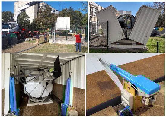
Figure 3.
CLUE container hosting the pBRL. (Top left): Container closed during transport. (Top right): Container opening. (Below left): Inside view of the container. (Below right): Actuator with motor and control box.
3.2. The Telescope Chassis and Petals
The CLUE telescope chassis is an alt-az mount designed to support a 1.8 m mirror and CLUE’s rather bulky focal plane instrumentation, see Figure 4. The movement of the telescope in both degrees of freedom is actuated by stepper motors of the model PH299-F4.0, manufactured by the company VEXTA (Japan, now called Oriental motor [58]) and mounted on the chassis. The motors actuate on different reductors, manufactured by the company Bonfiglioli [59] (Italy). Motor power is directed to the telescope through a timing belt. A toothed pulley is fixed to the axis of the reduction. The motion control was adapted from the original CLUE design, keeping the power drivers for the stepper motors.

Figure 4.
Left and middle pictures show the telescope chassis seen from the front and rear, respectively. On the right, the telescope laser arm. The main components of the telescope chassis and petals: the metal platform that supports the azimuth movement (a), the U-form structure that supports the elevationmovement (b), the focal plane support (c), the support for the small mirrors to align the laser beam (d), the structure for the laser arm (e), the petals covering the primary mirror (f), the cooling system of the laser (g) and the polychromator (h).
The chassis also supports a motorized protective foldable petals system and the optical system in the focal plane; see Figure 4. The empty metal square in the focal plane once held the CLUE multiwire camera, which has been removed. The petals are used to protect the primary mirror from dust. They are made of polystyrene and are actuated by four 12 V motors; the movement is controlled by eight series-connected limit switches. When the motor is operated, a long endless screw opens or closes the petal until the limit switch issues a signal. The laser arm visible on the right side of Figure 4 was added afterwards.
3.3. The Primary Mirror
The CLUE container was equipped with a 1.8 m diameter parabolic mirror of the same focal length (f/1), described by Alexandreas et al. [50]. It was produced following a hot slumping technique, first invented at CERN [60,61], and later adapted to the requirements of CLUE, especially the large mirror size. The mirror is made of smooth float glass produced by the company Società Italiana Vetri (SIVET, Porto Marghera, Italy), now called Pilkington Italia [62]. The glass has a low carbon content and a high chromium (0.5% C, 13% Cr) content and a thermal expansion coefficient of 8.5 × 10⁻⁶/°C. The glass is placed over a mould, with both heated in a large electric oven that reaches 600 °C at the company Sunglass [63] (Villafranca Padovana, Italy) so that the glass retains the shape of the mould. For this reason, the mould must be very precisely shaped. The mould was cast in a special stainless-steel alloy STAVAC ESR AISI 420 with thermal expansion coefficient (13 × 10−6/°C), comparable to that of the glass. The mould was machined to a concave parabolic shape with a digitally controlled lathe with nominal accuracy better than 20 µm. The deviation of the mould from the nominal parabolic surface and the glass plate defects introduced differences in the slope of the parabolic mirror of less than 1.6 mrad. These effects enlarged the image in the focal plane by 5.8 mm at maximum, when realized [50]. The mirror thickness amounts to 6 mm for a total weight of about 30 kg. Figure 5 shows a picture of the primary mirror.
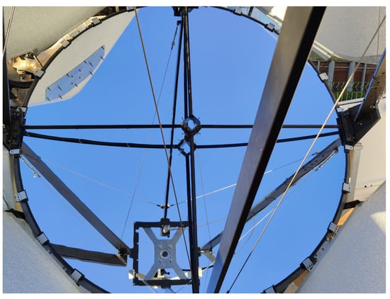
Figure 5.
A 1.8 m diameter parabolic mirror with f-number of one serves as the lidar’s primary mirror.
Point spread function. Alexandreas et al. [50] reported that 80% of the light of the eight original mirrors was contained within a square of 5–8 mm, depending on the mirror (more than nine were produced). Considering that the mirror had been inoperative for several years, we carried out new measurements to characterize the point spread function (PSF). The mirror spot size was then characterized by different methods, all producing compatible results. These were reported in more detail in [64,65].
For the most accurate of our tests, we created an artificial light source by pointing a green laser at a wall 65 m from the telescope to observe the backscattered light. The size of the laser spot on the wall was mm, which corresponds to 0.2 × 0.4 mrad at 65 m, similar to the 0.5 mrad of the actual pulsed laser employed by the pBRL. A diffusive millimetre paper was attached to the focal plane and a CANON EOS 1000D camera (https://www.canon.es/support/consumer/products/cameras/eos/eos-1000d.html?type=manuals&language=EN, accessed on 6 March 2025) was placed 25 cm behind the paper. The image was then fitted to a constant background plus a two-dimensional asymmetric Gaussian (see Equation (3) in a similar discussion in Section 3.9), characterized by two widths and , and a rotation angle. We then calculated the relative amount of light enclosed in ellipses of the same rotation angle and aspect ratio, with increasing distance from the centre (Figure 6, top). We found that ∼80% of the reflected light was contained in a pinhole of 4 mm radius (see Section 3.6), roughly compatible with the measurements made by the CLUE collaboration [50]. Unfortunately, after the pBRL returned from its one-year test period at the ORM (see Section 5), the point spread function had become significantly degraded (Figure 6, below), probably due to tensions applied to the mirror after inappropriate handling of the container by the various involved transport companies.
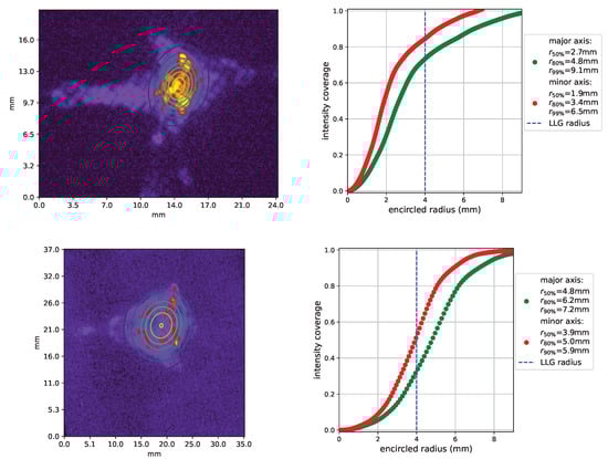
Figure 6.
Left: Spot size profiles with the elliptic contours of the two-dimensional Gaussian fitted to the image. Top: Image of a 65 m distant laser spot, from 2014. Below: Image of Venus, after the LIDAR had returned from its test campaign on La Palma. Note the different scales on the top and below plots. Right: Plots containing the relative amount of light enclosed within increasing-sized ellipses, characterized by a major axis (green) and minor axis (red), of the same rotation angle and aspect ratio, for each measurement, respectively. See the text for more details on the measurement.
Mirror Reflectivity and re-aluminization The original reflective coating of the mirror was a 50–100 nm layer of aluminium vacuum evaporated at the Osservatorio Astrofisico of the University of Padova (Asiago, Italy). After four years of operation, the mirror had lost reflectivity from originally 95% to 50–60% due to a missing protective coating and was realuminized at the William Herschel Telescope (WHT) [66] (Observatorio Roque de Los Muchachos, La Palma, Spain). The mirrors had again considerably degraded in reflectivity when acquired. The surfaces appeared milky and dusty. Focused reflectivity measurements were made showing values of only ∼(60–70)% at 350 nm [67]. The surface reflectivity was measured with a spectrophotometer. Many points in the mirror area were sampled locally, producing relative deviations <5%. Focused reflectivity was measured instead by estimating the sun light on a clear day concentrated on an aluminium plate placed in the focal plane and by evaluating the increase and decrease in plate temperature after opening and closing the mirror petals [67].
Although the focused reflectivity might have been acceptable for the pBRL, we decided to realuminize the mirror and add a quartz-protective coating. The mirror was sent to the company ZAOT [68] (Milan, Italy) in November 2020 for refurbishment, together with a second mirror belonging to IFAE and a third from the Laboratoire Univers et Particules de Montpellier (LUPM, France). With a coating of 150 nm on a substrate of aluminium, after realuminization, we expected (computed using the on-line tool https://www.filmetrics.com/reflectance-calculator, accessed on 6 March 2025) reflectivity values of 85%, 87%, 92% and 90%, respectively, for 355 nm, 387 nm, 532 nm and 607 nm for an angle of incidence of 10 degrees, which represents the average tilt of photons impinging the mirror. The coating thickness was optimized for the best reflectivity. We explored thicknesses between 100 and 250 nm and found maximum differences (peak to peak) in reflectance of 10% [69].
3.4. Telescope Optics Design
The CLUE telescope has a parabolic mirror surface of 1.8 m diameter and with a PSF of about 5 mm diameter for 80% containment (see also Section 3.3). This reflects into a telescope angular acceptance (or telescope “effective” field of view FoV) of PSF/f = 6/1800 = 3.3 mrad, which contains very well the light coming from the laser with a beam divergence angle of 0.5 mrad.
For the pBRL design, one possibility could have been placing the polychromator unit directly at the focal plane, but this was discarded because the size of the polychromator would have caused significant shadowing on the primary mirror. Instead, the most appropriate place to allocate the polychromator appeared to be the rear of the lidar mirror, where the mechanical structure is already well adapted to hold devices, as shown in Figure 7.
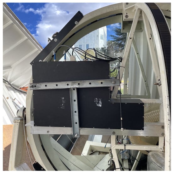
Figure 7.
The polychromator readout unit (black) is attached to the rear of the mechanical structure, behind the primary mirror.
The CLUE mirror exhibits, in its centre, a drilled hole of 50 mm diameter. The hole may allow the design of a double-mirror Cassegrain-like configuration, which redirects the light towards the rear of the primary mirror. This option has been explored in more detail. In that setup, the relatively small size of the hole may support a polychromator with a relatively small field stop, which in turn allows the use of moderately sized optical elements and the use of normal-sized photosensors, typical for lidars. We used a public version of ATMOS (https://www.atmos-software.it/Atmos8_96_FREE.html, accessed on 6 March 2025) that implements simple analytic calculations for the pre-design and later performed a full ray-tracing analysis using ZEMAX OpticStudio (https://www.ansys.com/products/optics-vr/ansys-zemax-opticstudio, accessed on 6 March 2025). Figure 8 shows two investigated designs of Cassegrain-like solutions. The input and output parameters of ATMOS are reported in Table 1.
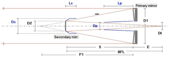
Figure 8.
Design scheme of a Cassegrain-like configuration for the CLUE telescope obtained with the public ATMOS code. All the input and derived parameters are shown in the Table 1.

Table 1.
Input and output parameters for the optical Cassegrain design obtained with the public ATMOS code.
Despite Cassegrain-like configurations being useful to make compact telescopes and reduce spherical aberration, they act like a zoom into the FoV of the primary mirror, i.e., they magnify the system: the spot size is seen to be enlarged with respect to the PSF of the primary mirror alone. Two magnification designs (8 and 30) are calculated in Table 1 as the ratio between the focal point of the system to the secondary distance and the distance from the secondary surface to the focal point of the primary , or the ratio between the effective focal length and the focal length of the primary mirror :
In the design with magnification , we attempted to minimize obscuration by having a small secondary mirror, thus providing a final PSF of about 18 cm, which not only would have required additional optics or a too-large polychromator unit but also would have implied considerable loss of light given that the central aperture on the primary mirror is only 5 cm. Finally, the diameter of the secondary mirror would have been 6 cm in this configuration, causing additional light shadowing of 3.5%.
Reversing the argument: To obtain an image of the primary PSF smaller than the rear hole, the magnification of the secondary mirror must not exceed , and therefore, the effective focal length should not exceed about 15 m. In this configuration, the diameter of the secondary mirror would be as large as 22 cm and hence produce a linear obstruction of about 12% of the light. In addition, the FoV of the telescope would be as large as mrad, probably covering a nonoptimal, too-large fraction of the sky. Given the problems in the two limit configurations considered and the additional mechanical problems related to the aligning of both mirrors in a stable way, in such a light structure as the one of the CLUE telescope, we decided to discard the Cassegrain-like configuration.
The alternative solution chosen consists of placing an optical fibre to collect light in the focal plane and transmit it to the polychromator unit mounted at the rear of the telescope (Figure 2). Given the size of the PSF and the dimensions of the telescope, a thick optical fibre of at least 6 mm diameter and over 3 m length was needed. Given that , a fibre with a numerical aperture (NA) greater than , with good transmission properties, was chosen in the wavelength range between 350 nm and 600 nm. The actual choice for this fibre and the optical elements required for its use with the polychromator system are deferred to Section 3.7.
3.5. Coaxial Laser Beam
LIDARs can be built in a coaxial (i.e., the laser beam is coincident with the telescope’s optical axis) or a biaxial design (the laser beam moves parallel to the optical axis of the light-capturing telescope). Coaxial LIDARs require dedicated steering optics to guide the laser beam towards the optical axis of the telescope. However, biaxial lasers require less hardware to align the laser beam and are easier to design at the expense of larger light loss for close-range sensing.
The range at which the atmosphere can be sensed is determined, at the near end, by the range of full overlap between the laser beam and the telescope’s field of view. The starting range of full overlap determines the minimum sounding range in the atmospheric boundary layer, a key design parameter for a lidar. It is usually lower for a coaxial lidar and higher for a biaxial lidar, typically several hundred meters to 1 km [70]. Below the full overlap range, the overlap function becomes smaller than one and can in principle be corrected [71]; however, the corrected data become increasingly noisier.
For a perfectly aligned biaxial lidar, the following formula can be used to estimate the distance of the full overlap range R [70]:
where x is the distance of the laser to the centre of the telescope mirror, d is the primary mirror diameter, D the radius of the focal plane detector and f the focal length of the telescope ( is also called the field of view of the detector). is the opening angle of the laser beam in radians. Note that in the case of , R does not get reduced to zero, due to the confusion circle of the source image, which becomes large at small distances if the telescope is focused at large distances or infinity. With our setup, with the assumption of a perfectly aligned biaxial laser located just at the edge of the telescope at m), with m, cm, m, mrad, Equation (2) yields 200 m. Nevertheless, also taking into account the aberrations of the telescope (not reflected in Equation (2)) makes a minimum achievable range of 400–500 m more realistic.
In the case of a coaxial lidar, R reduces to 80 m and 150 m for without and with aberrations, respectively. The choice of a coaxial system, as chosen for the pBRL, thus opens the range from 150 m to 500 m above ground for atmospheric characterization. Note that at astronomical sites during clear nights, the most important aerosol contributions are found within the first 500 m above ground. These aerosols are usually not turbulently mixed [11], and hence, a constant aerosol density does not correctly model the aerosol extinction profile.
3.6. Liquid Light Guide
A liquid light guide (LLG, see Figure 9) of type Lumatec Series 300 (https://www.lumatec.de/en/products/liquid-light-guide-series-300/, accessed on 6 March 2025), with fused silica window and fluoropolymer tubing, of 8 mm diameter and 3.2 m length, is used to transport the light from the focal plane to the polychromator unit. This model is optimized for the spectral range from 320 nm to 650 nm. The LLG has a numerical aperture (NA) of 0.59 (acceptance cone with a diameter of 72°, see Figure 9). The liquid inside the LLG remains stable for many years if the LLG is not exposed to radiation with wavelengths below 320 nm or above 650 nm. Shorter wavelengths may destroy the transmission properties of the liquid, whereas strong illumination by longer wavelengths may overheat the liquid and cause bubbles. Too sharp bending should be avoided; otherwise, the optical tube may kink and transmission will degrade permanently. The minimum bending radius is about 100 mm, coincident with the mechanical limit. The optical transmission may also degrade through improper handling, i.e., kinking, overheating, or by exposing it to a vacuum, arid climate, etc.
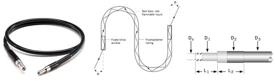
Figure 9.
The Lumatec series 300 liquid light guides (LLGs). The principle is illustrated in the central plot. The dimensions of the end fittings of the LLG: Active core (D0): 8 mm, end fittings: (D1): 10 mm, (L1): 20 mm, (D2): 15 mm, (L2): 40 mm, protective sleeve (D3): 12.5 mm. All images from [72].
LLG linear transmission. Peak transmission values of up to 80% can be obtained for LLG reference lengths of 2 m (see Figure 9 (left)). We carried out transmittance measurements with the 3.2 m LLG using a deuterium source, a Minolta CM100 monochromator and a Newport 818-UV light sensor in a dark room under controlled temperature and humidity [64]. The transmittance was measured from 300 nm to 600 nm in ON/OFF mode. The measurement was repeated 10 years after the purchase of the LLG. Figure 10 shows an overall agreement with the reference Lumatec data (measured at 2 m fibre length) and our measurements. Transmittances of ∼70% are found in the relevant wavelength range from 350 nm to 550 nm, and ∼45% for 607 nm. After ten years of operation, the transmittance has reduced to 50–60% for the UV and green wavelengths, but it has remained stable at 607 nm.
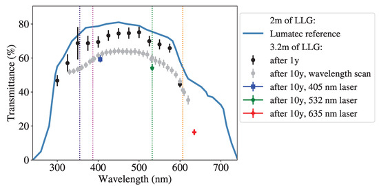
Figure 10.
Linear transmittance of the LLG. The solid blue line is taken from the datasheet of Lumatec for a reference LLG length of 2 m. Black points refer to our measurements for an LLG length of 3.2 m after one year from its purchase and in grey after 10 years of use. The blue, green and red markers indicate a separate measurement carried out with continuous wavelength lasers of 405 nm, 532 nm and 635 nm. The dotted coloured lines indicate the four wavelengths used for the pBRL.
LLG angular transmission. After testing the transmissivity of the LLG with respect to the incident angle, for these measurements, a class III green laser pointer was used as a light source. The laser is attached to a rotating support and placed at the entrance of the LLG. The output is measured from 0° to 60°, see Figure 11. It has been found that transmission from 15° to 30° decreases slightly and decreases by one order of magnitude from 30° to 35° [64]. This is sufficient for the design of the pBRL, since the maximum incidence angle of light reflected by the mirror towards the LLG is exactly 26.6°.

Figure 11.
Measured angular dependency of the transmissivity of green light through the LLG. The dashed blue line shows the maximum incidence angle of light from the primary mirror for reference.
LLG temperature-dependent transmission. For this test, the linear transmittance of the LLG was measured several times at room temperature, in order to obtain a reference for each wavelength. The LLG was then cooled to zero degrees with the help of ice and again measured several times. Finally, the LLG’s transmittance was measured again at room temperature. Figure 12 shows the transmittance ratios obtained for both temperatures. Although the cooling process did not affect the transmittance, reestablishing room temperature seemed to have reduced the transmittance by about 3%.
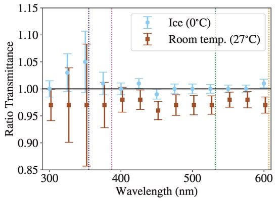
Figure 12.
Ratio of linear transmittance concerning original one at room temperature, as a function of wavelength. In blue, the transmittance ratio at 0 °C is shown, whereas in brown, the ones obtained after re-establishing room temperature. The error bars show statistical uncertainties only. The dotted coloured lines indicate the four wavelengths used for the pBRL.
LLG angular deviation and stability. The relation between the exit angle and the input angle for the LLG was measured using the same system as for the angular dependence of the transmissivity. A positive linear dependence was measured between these two angles, with a relation , consistent with expectations.
LLG fluorescence emission. LLGs can show fluorescence light emission shifted by (3474 ± 375) cm−1 [73] when illuminated by strong UV light. In our case, this would result in undesired secondary emission lines of (405 ± 6) nm and (653 ± 16) nm. Although no Raman line is found within these ranges, undesired fluorescence light leakage into these channels must be carefully avoided.
LLG shutter. The pBRL polychromator is operated such that the PMT high voltages (HVs) are ramped down whenever operations are finished, which is the case when ambient light levels become too high for the safety of the PMTs. In order to additionally protect the entrance of the LLG at the focal plane from spurious light and dust during non-operational times (e.g., during the day), a shutter system was included (see Figure 13). We designed a remote-controlled shutter that can be opened at the start of operations and closed at the end. We used the commercial Thorlabs stainless-steel diaphragm optical beam SHB1, 1″ diameter, equipped with a remote controller with TTL inputs and interlocks, and coupled to a 1″ long SM1S10 lens tube spacer. The system is mounted on a plate placed in the focal plane in front of the LLG entrance. The shutter can be operated up to a rate of 15 Hz, and is guaranteed up to 15 Mcycles. While the operating temperature specified by the manufacturer of the shutter is between 15 °C and 40 °C, the shutter was tested to perform flawlessly during a commissioning period at La Palma even at much lower temperatures. The LLG shutter has an angular acceptance of 30 degrees, which nicely coincides with the maximum angle under which the primary mirror is viewed, thus further reducing the stray light.
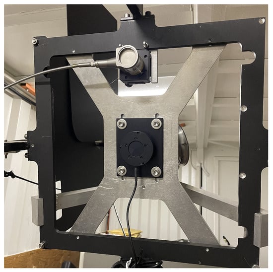
Figure 13.
Picture of the LLG shutter system installed in the centre of the focal plane of the lidar. The metallic structure holds the shutter in the centre. On the top part of the picture, the rear side of the near-range optics can be seen.
3.7. Optical Bench Polychromator
The optical bench (hereafter the polychromator) must collect and collimate the light transported by the LLG and successively separate the different wavelengths using dichroic mirrors and narrow-band filters. All glasses must be transparent to the four wavelengths used, particularly in the UV regime. Fused silica glass or N-BK7 are both good choices, while flint glasses normally used to design achromatic doublets cannot be adopted due to their poor UV transmission. The drivers for the design of the polychromator unit were: (a) to cope with the large aperture of the LLG, (b) to maintain optical elements within dimensions that are easily commercially available while limiting their number and (c) to maximize the collective effectiveness and global efficiency. Design choices were also driven by cost issues.
Polychromator design. We therefore defined the baseline design of the pBRL for four readout channels: two elastic, at 532 and 355 nm, and two Raman, at 387 and 607 nm.
Optical simulations were performed with the Zemax ray-tracing code. Table 2 shows the requirements for these simulations and the specifications of the optical elements used. The layout of the optical design of the polychromator is shown in Figure 14 (top). The light received by the telescope and transported by the LLG exits with a 70° aperture angle and is then collected by a system of lenses. To collimate such a diverging beam, a two-lens system is necessary. A three-lens system might also be used, at the expense of a decrease in the total efficiency of the system. For the sake of simplicity of procurement and to save costs, all lenses in the system are identical plano-convex lenses, made of N-BK7 glass, with a focal length of 150 mm and a diameter of 100 mm (https://www.lobre.it/en/home-english/, accessed on 6 March 2025). Fused silica glass would also have been an option with higher transmission but was discarded because it was more expensive. After collimation with the lens couple (LC) system, the light is separated into its different wavelength components via dichroic mirrors (DMs). A DM reflects light below a certain wavelength and transmits it above; therefore, the three DMs visible in Figure 14 are not identical. With three DMs, the four wavelengths can be completely separated. After this, a second LC focalizes the beam of each channel towards its photon detector, with an interposed interference filter (IF) for further suppression of light outside the desired respective wavelength window. Care was taken in the definition of the wavelength acceptance band for the DMs and the IFs since the light impinges onto them at various angles because of the aperture of the light beam. All IFs have been designed with a transmission > 85% centred on the corresponding channel wavelength and a transmission FWHM at 10 ± 2 nm around the central wavelength. Transmission outside the passband was specified to lie below 5%. IFs were acquired from the company Optics Balzer [74] (Liechtenstein). Measurements post delivery showed even better performance of <2% transmission outside the passband and >99% at the central wavelength plus/minus 2 nm. The DMs were custom-made by the company BTE [75] (Elsoff, Germany). They were required to have a transmittance better than 85% for the wavelengths of interest and absorption higher than 95% for the respective range of interest, as well as being optimized for <45° incident unpolarized light. The required size was mm. BTE proposed a Borofloat solution with a thickness of mm, edges cut, chamfered and a single-side coating matching our requirements. Figure 15 shows the transmission properties of the DMs as a function of the incident angles.
Table 2.
Requirements and design specifications for the optical design of the polychromator unit.
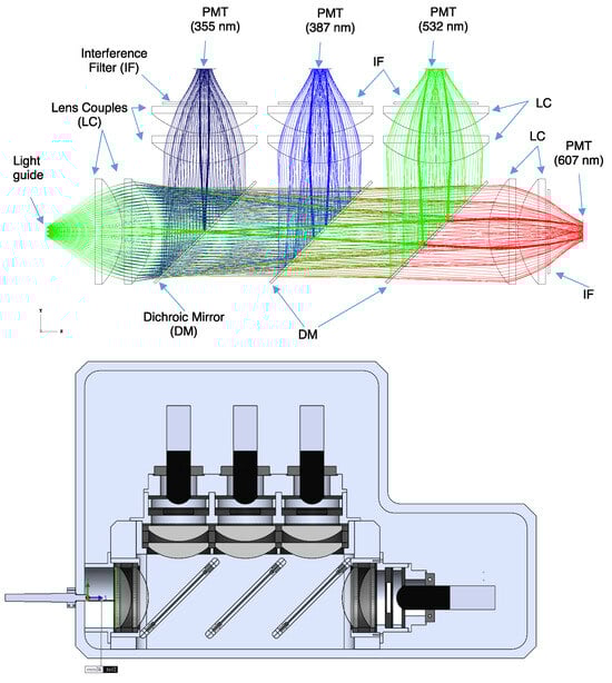
Figure 14.
The polychromator ZEMAX design and sketch of the optical bench. The dichroic mirrors, the interference filters and the converging lens doublet system are shown. The design was described in Da Deppo et al. [76].
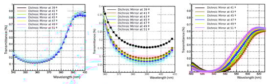
Figure 15.
Dependency of the transmission properties of the dichroic mirrors on the incidence angle. Left: for 355 nm, centre: for 387 nm and right: for 532 nm.
In Figure 16 (left), the footprint of five sample points simulated by Zemax, one in the centre and four at the edges of the input optical fibre, is shown together with a circle corresponding to the 22 mm active area of the PMT detector. In Figure 16 (right), the enclosed energy fraction calculated for a uniform circular object of 8 mm in diameter, such as the input fibre, is shown. The total energy emitted by the fibre is collected and focalized on the PMT area.
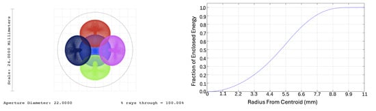
Figure 16.
Left: Footprint diagram of the PMT active area. Right: Encircled energy diagram of the PMT active area.
Finally, Figure 17 shows the mechanical design of the polychromator developed in the IFAE engineering division.

Figure 17.
Design of the polychromator (left) and the PMT holder (right).
Light leakage tests. Light leakage tests are used to control whether the Raman signals, which are more than two orders of magnitude dimmer than the elastic signals, may be affected by external or internal leakage of light. For the tests, the collimated light from a stabilized Xenon lamp was wavelength-selected with the help of a grating monochromator. To discriminate unwanted harmonics, the light was first passed through a broadband filter. A shutter allows remote switching on and off of the monochromatic light. The light was then fed into the LLG and coupled to the polychromator unit (see Figure 18). Finally, PMT currents were recorded using a picoammeter. Series of measurements with an open shutter were taken, immediately followed by background estimates using the closed shutter, until sufficient statistics had been accumulated.

Figure 18.
Sketch of the setup for polychromator tests: the light of a calibrated Xenon lamp passes through a collimator and a filter wheel with either an empty hole or a broadband filter. Then, it passes through a grating monochromator and a shutter and gets coupled to the LLG, which is connected at the other end to the polychromator unit. The current of the four PMTs is read out by a picoammeter (not shown in the figure).
Figure 19 shows the measurements made for a full-wavelength scan from 300 nm to 650 nm. The individual measurement points have been corrected for the Xenon lamp spectrum to match the polychromator’s response to a flat photon spectrum. Nevertheless, the tiny background-subtracted currents far from the main response peaks may be inaccurate in this figure, because of the relatively long duration of the full-wavelength scan, followed by the background measurements with the closed shutter. Furthermore, slight changes in background PMT currents were observed with different filter wheel settings (changed at 600 nm), which add to the inaccuracy of the small residual currents.
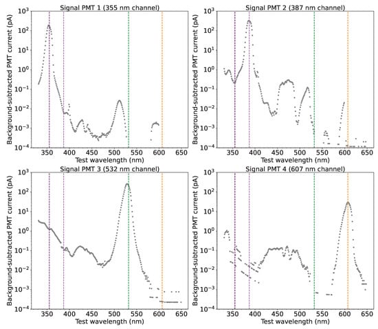
Figure 19.
Results of a wavelength scan for the four channels. The dashed coloured lines show the four LIDAR wavelengths.
To address these issues, improved measurements were designed specifically for the light leakage from the strong elastic lines into the Raman channels. Figure 20 shows measurements made with the PMTs of the 387 nm and 607 nm Raman channels to test the presence of additional PMT currents when the polychromator is illuminated with wavelengths around 355 nm and 532 nm. Figure 20 (top) shows the observed relative part of the signal from the elastic channels leaking into the 387 nm Raman channel. Likewise, Figure 20 (below) shows the results of the 607 nm Raman channel. We observe a residual light leakage of (6.5 ± 0.2) × 10−6 from the 355 nm elastic line into the 387 nm Raman channel and (3 ± 1) × 10−6 from the 532 nm elastic line into the 387 nm Raman channel, respectively. Leakage from the elastic lines into the 607 nm channel was not observed and can be excluded above 3 × 10⁻⁶ (95% CL) from both elastic lines.
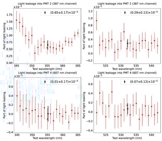
Figure 20.
Results of a wavelength scan around the elastic lines (355 nm, left, and 532 nm, right) for the two Raman channels (387 nm, top, 607 nm, below). The black entries show the weighted average of ten entries around the central elastic wavelength.
We collect several transmittance factors contributing to the light collection efficiency of the polychromator in Table 3. We report the mirror reflectivity, the light transmittance of the LLG, the dichroic mirrors and the interference filters, as well as the photon detection efficiency (PDE) of the PMTs. We compute the total transmittance and its uncertainty from these values.
Table 3.
Transmittance parameters for the wavelengths of interests.
Photomultiplier tube photosensors. Lidars require photon counting and signal amplification. The custom solution is based on the use of photomultiplier tubes ((PMTs). However, the supremacy of PMTs is currently being challenged by photon sensors rapidly spreading in popularity, the silicon photomultipliers (SiPMs), which are becoming a valid alternative because of their high photon detection efficiency, low operating voltage and installation flexibility. SiPMs are photosensors composed of microscopic diode cells assembled in matrices of thousands to reach sizes of a few millimetres in diameter. In comparison to PMTs, in addition to their low operating voltage, they provide additional advantages such as high efficiency, insensitivity to magnetic fields and robustness against bright ambient light. Their main drawbacks are their small size, higher optical cross-talk, longer signal duration, temperature dependence and sensitivity to red light compared to PMTs.
Considering that the photon beam opens up widely on its way from the focal plane through the polychromator, a sensitive area of the order of a few cm2 is required. Currently, single SiPM matrices can hardly reach 1 cm2. The combination of several SiPMs, albeit possible, would require a complication in terms of electronics, which led us to discard this option in favour of the traditional PMT. For the choice of PMTs, we chose those in use in actual IACTs, specifically those chosen for the first Large Size Telescope (LST1) of CTAO, under construction at the ORM at the time of purchase. Their sensitivity overlaps with our wavelength range of interest. This guaranteed reduced acquisition and characterization costs. The pBRL used three identical Hamamatsu 8-dynode PMTs of type R11920-100-20 [78] for the UV and green lines (see Figure 21 (left)). A second PMT type, the Hamamatsu H10425-01 (https://www.hamamatsu.com/eu/en/product/optical-sensors/pmt/pmt-module/current-output-type/H10425-01.html, accessed on 6 March 2025) has been purchased for the red line at 607 nm but not yet integrated into the system. Since the polychromator system had been designed for 1.5″ PMTs, the latter was also selected to be of the same size but with a higher quantum efficiency at 607 nm. Table 4 summarizes several technical parameters of the R11920-100-20 PMT.

Figure 21.
Top left: A picture of the Hamamatsu R11920-100. Top right: A photo of the PMTs inside the polychromator. Below: The light concentrated onto the PMT photocathodes.
Table 4.
Selection of technical properties of the PMT Hamamatsu R11920-100-20.
Polychromator assembly. The polychromator was built and assembled at the IFAE engineering division. It is housed in a large box with dimensions of 760 mm × 550 mm × 170 mm, and is additionally enclosed in an aluminium outer box that prevents the possible leakage of stray light into the unit and protects it from electronic noise. Together with the optical system and the photomultipliers, the entire unit weighs about 30 kg.
The polychromator unit has five connectors: a separate coaxial connector for the signal line of each of the four PMTs and a DS9 connector, which carries the 5 V and GND feeding lines, plus the four control voltage lines for the PMTs.
The signal lines are connected to the readout electronics through 10 m coaxial cables. In a previous version of the pBRL, the signals were preamplified by a factor of 10 and deamplified again before entering the readout, a solution later discarded given the relatively large pulse width of the single photoelectron produced by the Hamamatsu R11920.
The control voltages of the PMTs are produced by a separate small electronic unit carrying corresponding digital-to-analogue converters (DACs), which allow user-controlled setting of the HV of each PMT individually.
3.8. Readout Electronics
Although the readout electronics can be custom-made, the Licel company [79] (Berlin, Germany) offers a highly successful commercial solution. The Licel Optical Transient Recorder (LOTR) is a powerful data acquisition system, specially designed for remote sensing applications. Table 5 summarizes the LOTR specifications provided by the manufacturer.
Table 5.
Licel Optical Transient Recorder specifications for the 20 MHz recorders. In brackets are the values corresponding to the newer 40 MHz modules.
The LOTR is made up of a fast transient digitiser with onboard signal averaging, a discriminator for single-photon detection and a multichannel scaler combined with preamplifiers for both systems. For analog detection, the signal is amplified and digitized by an A/D converter. A hardware adder is used to write the summed signal into a 24-bit wide RAM. Three LOTR versions have been purchased: a 12-bit-20 MHz recorder for the 355 nm channel, a 16-bit-20 MHz for the 387 nm Raman line and 16-bit-40 MHz versions for the other lines. The latter two also register the standard deviation of the analogue signal. The signal part in the high-frequency domain is amplified and a 250 (800) MHz fast discriminator detects single-photon events above a selectable discriminator threshold voltage ranging from 0 to −25 mV in 64 steps for the 12-bit-20 MHz (16-bit-40 MHz) version, respectively. The photon counting signal is written to a 16-bit wide summation RAM which allows averaging of up to 4094 acquisition cycles. A time resolution of 50 (25) ns without any dead time or overlap between two memory bins is reached by using a continuous counter together with a multichannel scaler of an ASIC custom designed by the provider.
The LOTR is completely software controlled and interfaced by a custom-written software module of the LIDAR Client (LICLI) programmed in Java SE 21. Input ranges for analogue and photon counting acquisition, discriminator levels and the number of active bins can be selected. The acquired analogue and photon counting signals for both summation memories can be read out separately. Data are transferred via a 2 × 16 bit interface to a National Instruments DIO-32-HS family (PC) interface card. A custom Python 3.10 interface was created to read, convert into FITS [80] format and visualize the data.
3.9. The Laser
The pBRL uses a Brilliant Nd:YAG laser from the company Quantel [81] (France). It is a pulsed 10 Hz flashlight-pumped and actively Q-switched class IV laser with a fundamental wavelength of 1064 nm and energy per pulse of up to 400 mJ. The pulse intensity can be changed by the user through manipulation of the Pockels cell Q-switch delay. A second and third harmonic generator at 532 nm (200 mJ per pulse) and 355 nm (100 mJ per pulse) are added to the main body of the laser. They are assembled in compact modules, including the nonlinear crystals and a removable set of dichroic mirrors. Phase matching for the second and third harmonics is obtained by a simple mechanical adjustment (adjustment screw accessible from the top of the module). For the pBRL application, we are only interested in the second and third harmonics, which exit the laser coaxially. Since there is no automatic way to mask the 1064 nm pulse, a configuration has been chosen where all three wavelengths exit the same output hole. In a later stage, the undesired 1064 nm line is therefore removed by the two dichroic guiding mirrors; see Section 3.10. The general characteristics of the laser are collected in Table 6 and Table 7. Since its purchase in 2010, the laser was maintained several times: the flashlamp needed to be replaced once, and the deionized water and filters were exchanged three times. The laser broke and was repaired in 2017 by the company Proton Laser (Barcelona, Spain; Proton Laser Applications S. L. has ceased to exist), who also measured that the output power had dropped to 250 mJ per pulse at 1064 nm.
Table 6.
Main characteristics of the pBRL Brilliant Nd:YAG laser from the Quantel company.
Table 7.
Characteristics for main pulse and harmonics.
Temperature Control. The laser head is a monolithic, temperature-stabilized block which ensures the alignment of the resonator mirrors. The temperature is controlled by a water loop that goes through a water/air heat exchanger. The cooling group is an independent unit that cools the systems using a closed loop of deionized water. This temperature-regulated water also provides thermal stabilization ±1 °C of the oscillator structure. For proper operation of the laser, the ambient temperature should lie between 18 °C and 28 °C. Quantel does not guarantee that beam quality stays within specifications outside this temperature range. Because the pBRL is regularly operated at night at ambient temperatures well below 18 °C, falling even below 0 °C, we equipped the system with additional heating, which can be optionally operated when the temperatures are so low that the cooling group unit could not heat the water to its operating temperature. The heater consists of a 3700 W Hotwind system from the company Leister Process Heat [82] (Switzerland) with a stepless adjustable heat output and air volume through a potentiometer. The industrial hot air blower is fed into a hose that delivers warm air both to the cooling unit and to the laser head (see Figure 22 (right)). During operation, the system is only turned on to speed up the cooling unit, achieving the operating temperature during cold nights. Once that temperature is achieved, the industrial hot air blower is automatically switched off, allowing the cooling group unit to maintain the water temperature without further assistance, even during freezing nights.
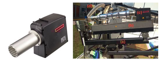
Figure 22.
Left: The industrial hot air blower system. Right: Picture of the laser arm: (a) laser arm structure, (b) laser head housing, (c) hot air blower and (d) laser cooling unit heating hose.
Near-field spot size. The waist diameter of the beam, according to the manufacturer, is 6 mm at 1064 nm. As we are mainly interested in the second (532 nm) and third (355 nm) harmonics, we measured the spot size in the near-field at these two wavelengths. Measurements were carried out by pointing the laser at a lead target at about 2.5 m distance and capturing the images with a Canon EOS 1000D camera [65], which were later digitized, each pixel was assigned a distance, and numerical integrals were performed to obtain a measurement of the relative amount of encircled energy [65].
For the 355 nm (532 nm) wavelength, about 80% of the light is enclosed in a circle of 2.6 mm (3.6 mm) of diameter, and 90% falls in a circular shape of about 3 mm diameter (4 mm). Most of the light (99.9%) is contained in a spot not much larger than 4 mm (5 mm) in diameter. The spot profiles are shown in Figure 23.
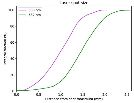
Figure 23.
Spot size for the 355 nm and 532 nm lines of the Brilliant laser.
Far-field beam divergence. The beam divergence test was carried out at the bus terminal of the Universitat Autònoma de Barcelona Campus where it was possible to reach distances larger than 80 m between the laser and a target sheet of graph paper mounted on a white panel. Pictures of the laser signal reflected on the paper were taken in RAW mode with a Canon EOS 1000D and a Nikon D5000 (https://www.nikon.com/, accessed on 6 March 2025). The beam spot was observed from very small angles concerning the perpendicular incidence. A Neutral Density (ND) filter was added in front of the camera to avoid saturation of the images. Only the Bayer-Green points were extracted from non-saturated pictures. All image pixels were converted to physical units by comparing the distance in image pixels of the outer edges of the white panel with its measured real size. The analysis algorithm (script available at https://github.com/mgaug/LIDAR-tools/blob/main/diameters_from_image.py, accessed on 6 March 2025) is described in the following [83].
A perfectly Gaussian beam produces irradiance that decreases monotonically with radius from the beam axis. In the case of real laser beams, the irradiance may not be uniform around the beam axis, introducing some arbitrariness in the definition of the beam profile. We used here a definition of the beam diameter that is based on the concept of encircled energy: the major and minor axes of an ellipse around a central point at which the encircled energy (expressed as summed and background-subtracted) image content has fallen to (1−1/) of the total.
The analysis algorithm was designed to fit such ellipses to the images. First, the images were fitted with a two-dimensional asymmetric Gaussian of height , with variable centre coordinates and , the widths of the major and minor axes, , and a rotation angle , plus an offset :
with:
The background was evaluated considering the outside regions of the fitted ellipse, at 5 from the centre, up to a suitably chosen cut-off point of the image. The cutout was chosen by eye on the basis of a constant number of entries, coinciding with a constant image colour. After subtraction of the background, the image was normalized and integrated into ellipses of the same axis ratio and rotation angle from () to the point where the integral reaches . At that point, the major and minor axes were evaluated. Subsequently, the full-angle beam divergences were calculated. Finally, the same procedure was used for ellipses of any size (always with the same axis ratio, rotation angle and centre) and the image intensity was computed for ellipses of increasing half-axes (see Figure 24).
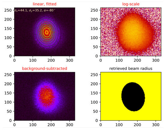
Figure 24.
The upper left part shows a laser spot image in linear scale, fitted with the 2D-elliptic Gaussian. The upper right picture presents the same plot on a logarithmic scale and without the retrieved concentric ellipses. The lower left panel shows the background-subtracted image and the lower right displays the ellipse that contains of the total normalized distribution.
Table 8 shows the results of the analysis of the full sample of images taken from the laser spot.
Table 8.
Results of the eight non-saturated laser spot images analysed in the far field: major axis of the spot ellipse (), beam divergence along the major axis (), minor axis of the spot ellipse (), beam divergence along the minor axis (), rotation angle of the ellipse (). See Maggio [83] for further details.
The beam divergences were measured at different laser intensities. We observed that the beam divergences obtained are significantly larger (by a factor of 2.6 along the major axis, and a factor of 1.7 wider along the minor axis) than the ones claimed by the manufacturer (unless the absolutely lowest laser intensity was used). The ratio between the major and minor axes is greater than 1.25 and increases as the laser intensity becomes lower. Moreover, the beam appears rotated by about 10° with respect to the vertical axis.
The degradation in beam quality might have been due to the repair carried out in 2017. Since we did not test the beam quality in the far field before the laser repair, we cannot compare with its original quality. The measured beam shape divergence increases the distance to full overlap of the pBRL by up to 150 m, as shown in Figure 25 (right).
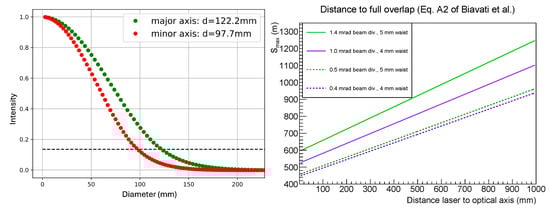
Figure 25.
Left: Intensity coverage of the background-subtracted and normalized medium-intensity non-saturated image, as a function of the fitted ellipse’s major and minor axes. The dashed black line shows , which is the nominal reference for the opening angle of a Gaussian laser beam. Right: Distance to full overlap [70] for the green and UV elastic lines, for the nominal laser beam divergences (dashed lines) and the measured ones (full lines).
Laser arm.Figure 26 shows the laser arm designed to control the correct alignment between the laser and the telescope. It is based on an table, designed to point with a precision better than 1 mrad. To move two different axes, two DC motors of type Faulhaber 3863H024C are attached to an endless screw of 1 cm/rev, one for each degree of freedom, controlled by encoder of type Faulhaber HEDL5540. A 111:1 reduction is used to improve the resolution. To fix the initial position of the table, two final switches are used. To control the entire laser arm, a control board with Ethernet interface has been developed.
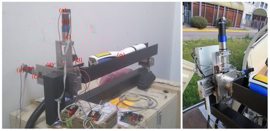
Figure 26.
Left: The laser arm in the laboratory: the encoder (a), the motors (b), the 111:1 reduction (c), the final switches (d), the driver (e), the control board (f) and the laser arm control (g). Right: The laser arm mounted on the telescope.
3.10. The Laser Dichroic Guiding Mirrors
The laser is mounted on one side of the telescope structure (see Figure 2) at about 1.1 m distance from the optical axis of the telescope. In order to make the laser light coaxial, we engineered a guiding arm system completed with mirrors to guide the laser light. This system also allows for (a) precise adjustment of the laser beam orientation and (b) filtering of the laser 1064 nm line, which may damage the light guide (see Section 3.6).
The arm holds the guiding mirrors and connects with the focal plane. For simplicity, the exact inclination of these mirrors needs to be adjusted by hand and fixed with screws. Space restrictions inside the container did not allow us to have a perpendicular design, and the arms are mounted at specific angles of 61.1 ± 0.3° (see Figure 2).
We purchased standard 1" fused silica mirrors of type MI1050-SBB (surface flatness l/10, damage threshold of >1 J cm−2 at 355 nm and reflectivity >99% (see Figure 27 (left) and [84]) from the company Precision Photonics [85] (Boulder, CO, USA; the company was purchased in 2012 by IDEX coorporation [86] (Northbrook, IL, USA)). We realized, however, that mirrors of only 1" diameter were insufficient to allow carrying out a pre-alignment of the laser beam (see also Section 4.1), particularly because the second dichroic allowed only a margin of ∼5 mrad for the fine adjustment by the remote-controlled laser arm. The beam needed to be pre-adjusted to that precision beforehand by manual movement of the mirrors, a task impossible to achieve in one night, even by an experienced person. After a thorough study [87], we found that a mirror of at least 10 cm diameter was necessary to achieve the required mrad margin of operation for the pre-alignment.
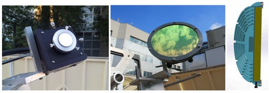
Figure 27.
Pictures of the first guiding mirror 1″ fused silica mirrors of type MI1050-SBB (left) and the final custom-made ones (centre). Right: Design of the guiding mirror holder, with heat dissipator.
The final 5″ diameter dichroic guiding mirrors have been designed such that they resist high laser power, have reflectivity >97% for the 355 nm and 532 nm wavelengths at an angle of incidence of 61° (see Figure 28) and a transmission >80% at 1064 nm and high surface flatness over 2″ and surface quality 20–10. The dichroic mirrors were designed by the company Optoprim [88] (Milano, Italy) and manufactured by the company Laser Components [89] (Olching, Germany). Figure 28 shows the final transmission spectrum achieved from guide mirrors, which is much higher than the requirements. The mirrors were mounted on a metallic custom-designed structure by the IFAE engineering division and allowed the adjustment of the mirrors on two axes by hand.
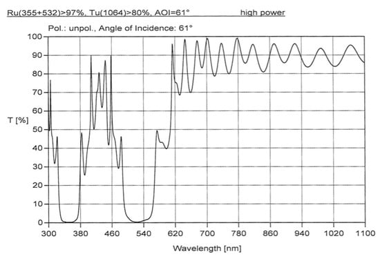
Figure 28.
Transmission of the dichroic guide mirrors, as a function of wavelength.
3.11. Stability of the Guide Mirror Structure and Mount
The stability of the structure holding the dichroic guide mirrors was tested for telescope movements in elevation and azimuth, as well as for different temperatures [87].
For these tests, we placed a millimetre paper in front of the second guide mirror and fixed it so that it did not move during the tests. Then, the centre of the laser spot was marked on the millimetre paper when the telescope was in the parking position. Throughout all tests, the same position of the XY table was maintained, as will be the case during normal operation, once the system has been aligned.
The tests consisted of taking photographs from the laser spot at varying telescope elevation positions and fixed azimuth and at varying telescope azimuth positions at fixed elevation angles. We observed that varying the elevation angle by 70° led to a movement of the laser spot by up to 4.5 mm, corresponding to 4.5 mm/(0.84 m + 1.3 m) ≈ 2 mrad, i.e., slightly less than half the field of view of the LLG pinhole. These movements were also tested for possible hysteresis or temperature dependencies, but none could be detected within the sensitivity limit of 1 mm, i.e., 0.5 mrad. The exact displacement could be reproduced after several days. No movement of the laser spot could be detected during an approximately 250° rotation in azimuth executed, leading to a limit of <1 mm, corresponding to <0.5 mrad. In addition, in this case, no hysteresis could be detected.
All in all, beam alignment may be necessary to be carried out at various elevation angles, and the results stored in lookup tables to correct for the observed sagging of the arm. Movements in azimuth should not cause any alteration in the alignment.
3.12. Short-Range System
In order to increase sensitivity at distances below 500 m from the ground where most of the aerosols of the nocturnal boundary layer are found with an approximately exponential decrease in density with height at the ORM [11], in a range where the signals are already strongly affected by saturation, the pBRL has been equipped with additional near-range optics. The near-range optics is composed of a Thorlabs RC12SMA-F01 mini-telescope (https://www.thorlabs.com/thorproduct.cfm?partnumber=RC12SMA-F01, accessed on 6 March 2025) held by a standard mount KM100T (https://www.thorlabs.de/thorproduct.cfm?partnumber=KM100T, accessed on 6 March 2025) (see Figure 29 and Figure 30). The near-range mini-telescope collimator is composed of a parabolic mirror used to focus light onto a 1.5 mm optical fibre of type FT1500 UMT (https://www.thorlabs.com/thorproduct.cfm?partnumber=FT1500UMT, accessed on 6 March 2025) (NA: 0.39, transmission from 300 nm to 1200 nm) screwed to the collimator with an SMA connector. The fibre transmits the signal to a PMT housed within a protective box with interference filter [90]. The box allows placing up to two interference filters in front of the PMT and hence makes it suitable to observe one of the two elastic lines.
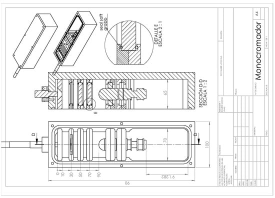
Figure 29.
Design of the protective box for the near-range optics and PMT.

Figure 30.
Components of the near-range system. The parabolic mirror (left), the support to mount the mirror on the telescope structure (centre) and the near-range PMT housed in a protective box (right).
With a field-of-view of ∼30 mrad, the near-range system can achieve full overlap basically from a few meters of distance [70].
4. Commissioning, Calibration and Monitoring
In Section 3, we have detailed the technological aspects of the pBRL. In this section, we discuss activities needed to characterize or calibrate the pBRL as a whole before putting it into operation.
4.1. Calibration of the Pointing and Beam Alignment
The alignment procedure must be performed during the night and takes about two hours. It requires a sheet of white paper, a set of Allen keys and an oscilloscope. A dedicated black light protection shield has been developed for the purpose of beam alignment, which protects the surroundings from spurious laser light (see Figure 31, left).

Figure 31.
Left: Picture of the black protection shield deployed to alignment position. Right: Picture of the first dichroic mirror with its fixation pole (lower left part of the image). The screw to loosen the movement of the pole and mirror is found on the aluminium ring surrounding the pole, visible on the very lower left part of the image.
First, the telescope has to be moved to the lowest elevation (highest zenith) allowed by the end-switch to operate the laser, and the laser has to be operated at the lowest light intensity. That intensity can be considered eye-safe. With the white paper and the low-power laser beam, the first laser guide dichroic mirror is aligned by hand using its fixation screws (see Figure 31, right) to point the laser beam towards the centre of the second guide mirror.
Subsequently, the telescope is moved to 90° elevation and the laser intensity is turned to 100%. With this, a vertical green laser beam is visible to the eye in the atmosphere above the telescope (see Figure 32). If the telescope is exactly pointing to the zenith, a possible inclination of the laser beam can be discerned by the human eye, and in such a case, the second dichroic guide mirror must be slightly moved into the opposite direction after the laser is switched off and the telescope has been moved into parking position again. This step may be repeated several times until the beam is found to exit the telescope exactly vertically.
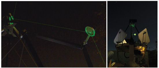
Figure 32.
Images of the laser light path visible during beam alignment.
At this point of provisional alignment, the 355 nm elastic line cable exiting the polychromator unit shall be monitored with an oscilloscope (see Figure 33). A strong direct backscatter pulse from the light scattering 3–4 times off the optical and mechanical elements of the LIDAR and ending in the LLG pinhole can always be seen if the PMT is operative.
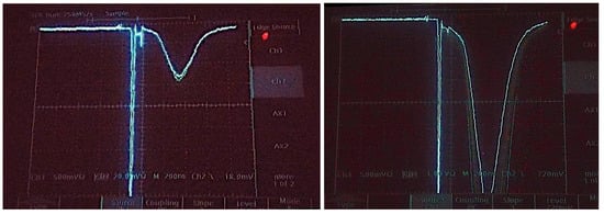
Figure 33.
Pictures of the oscilloscope signal, before the LIDAR is fully aligned (left) and once it is aligned (right). The first short pulse is due to multiple reflections of the laser beam on the different telescope parts, of which a part finally ends up in the focal point.
From that moment on, the laser arm can be moved remotely and the backscatter signal increased. Since the LIDAR is coaxial, there is always a small backscatter signal visible, which increases with better alignment, even in the absence of clouds. At a given moment, the signal “explodes”, that is, when the LIDAR starts to become aligned. From then on, the right (far-distance) part of the signal can still be increased until it reaches a maximum. Unfortunately, sometimes that part of the alignment procedure leads to the laser spot moving towards the edge of the second dichroic guide mirror. In such a case, if the beam is found to exit the lower part of the second dichroic guide mirror, that mirror needs to be moved slightly to the lower side, i.e., counter-clockwise. In contrast, if the beam exits the second dichroic on the upper edge, the mirror needs to be rotated clockwise. That procedure is followed with both axes of the XY table moving the laser arm until the backscatter signal is maximum, and both axes can be moved by about the same range until the signal starts to decrease. This range is about 300,000 steps wide.
A similar procedure involving only remotely controlled movements of the XY table controlling the laser arm can be followed for different telescope elevation angles, and the lookup table for the elevation-dependent alignment generated.
We observed that such an alignment remained stable during several months of operation under conditions of varying temperature and humidity; hence, the procedure is tedious but once achieved, stable.
4.2. Calibration of the Timing
The pBRL readout is triggered by the Q-switch of the laser, which our Brilliant model allows us to use for external triggering of the Licel readout. The trigger signal is the same for all readout modules. Therefore, one could expect that all channels provide a signal with exactly the same time offset. Unfortunately, this is not the case: we observed up to half a microsecond difference in the internal time delay between the 12-bit and the 16-bit models in the analogue line, and up to 100 ns in the photon counting lines. Within a same Licel Optical Transient Recorder (LOTR), the internal time delay between the readout of the analogue and photon counting readout may amount to up to half a microsecond for the old 20-MSample models, but less than 50 ns for the new 40-MSample modules, which shows a considerable improvement.
Given that the light path from the laser to the dichroic guide mirrors is unprotected, a strong signal pulse is recorded at time due to multiple scattering of the light from the guide mirrors towards the primary mirror structure. Even if only a tiny part of the laser light ends up in the LLG, a strong peak is nevertheless observed (see Figure 33) marking the signal start. That peak is visible in the amplitude recording, but not in the photon counting channel, where the signal readout starts a few tens of nanoseconds after that peak. For this reason, the direct laser backscatter peak serves for absolute calibration of the all-time delays, but not for the relative ones, for which clouds visible in both analogue and photon channels are needed.
4.3. Calibration of the Telescope Pointing
The telescope’s position is controlled by two 12-bit shaft encoders (SEs), one for each axis. This leads to an angular step size of per SE step. Nevertheless, an absolute calibration is necessary. The calibration of the shaft encoder values on the altitude axis was performed with an inclinometer with an accuracy of about 0.5° located on the main arm, which holds the plate in the focal plane. A scan through different altitudes yields the calibration recovered, shown by the red points in Figure 34. A fit with fixed slope yielded a /NDF of 0.71, compatible with the data. To test for possible sagging of the telescope structure, a fit with variable slope was also tried, which yielded per SE step, 1.8 standard deviations from the expected value of 0.0879 and a marginally improved /NDF of 0.66, hinting at negligible sagging of the telescope structure. That calibration has a precision of better than 0.2° and an accuracy of 0.5°. Its accuracy can be improved by pointing the telescope at Polaris in such a way that its image is correctly centred at the focal point.
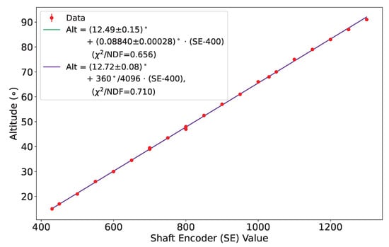
Figure 34.
Calibration of the telescope altitude vs. the altitude motor’s shaft encoder values.
4.4. Calibration of the Discriminator Thresholds
To calibrate the discriminator thresholds, we used the pulse height distribution method as suggested by Licel (see, e.g., https://licel.com/pulseheight.html, accessed on 6 March 2025). For this purpose, a stable UV LED was located in front of the pBRL’s focal point (see Figure 35 (left)), and average photon counting rates were recorded, as a function of the discriminator threshold. Licel [79] recommends using, as a starting point, a discriminator level of 8 (corresponding to ∼3 mV), suitable for PMTs with a typical gain of ∼106 for LIDAR applications. However, our PMTs were designed for a different purpose [91] and have a factor of approximately 4–5 lower gain. This has led to an optimum discriminator setting between 1 and 2 (see Figure 35 (right)), at the edge of the possibilities of the LOTR. The photon-counting channel is still operational at such low discriminator levels, due to the even lower PMT and electronic noise levels.
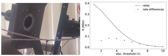
Figure 35.
Left: Picture of the setup used to calibrate discriminator setting. Right: A rate scan of one of the channels; the mean single photo-electron pulse height is found at around a discriminator threshold of 3–4.
4.5. Monitoring of the Telescope Reflectivity
Even with a proper coating, the overall reflectivity of the mirror is subject to degradation. If a coating of quartz is applied, this degradation should not exceed a few percent per year; however, this number depends on the quality of the coating. In general, it is advisable to calibrate the mirror reflectivity over time, of the order of once every few months. In order to do so, one can easily measure the surface reflectivity (as opposed to the on-focus reflectivity). The reason is that for surfaces with small roughness, as this mirror is (and in general solid glass mirrors are), the surface reflectivity is a good estimator of the on-focus reflectivity. Possible dispersion of light out of the focal spot is, on the contrary, more complex to measure because of the calibration of the setup for this measurement.
5. pBRL Operation
After being awarded the status of a CTAO Pathfinder, the pBRL was operated from March 2021 to April 2022 at the Observatorio Roque de Los Muchachos (ORM) on the Canary Island of La Palma (Spain). It was located within the restricted area of the LST1 telescope [92]. This location was chosen because of existing infrastructure, such as flat terrain in a fenced area, easy access to power and the network. The pBRL was set so that no interference was possible with the operation of the LST1 telescope, which included additional limit switches for the movement of the telescope to prevent any laser light from hitting the telescope or the camera access tower. Moreover, operation of the pBRL was only allowed during moonlit nights when the LST1 did not make observations.
Additionally, in order to avoid interference with other telescopes at the ORM, any operation of the pBRL that involved laser shooting was granted only during the evening, no later than 10 min before astronomical twilight, or in the morning, starting 10 min after astronomical twilight. Although the pBRL was fully operable from within the container, for the comfort of the operators, a semi-remote connection was established to the Counting House of the nearby MAGIC telescopes [93]. The LST consortium allowed us also to install monitoring webcams for improved safety of the semi-remote operations. A photo of the pBRL deployed in the LST1 area is shown in Figure 36.
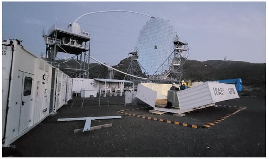
Figure 36.
A photo of the pBRL deployed into the LST1 area with the container open.
After the end of the pBRL test phase at the ORM, the system was prepared for transport back to the campus of the Universitat Autònoma de Barcelona. In the following subsections, basic information about the pBRL operation is provided.
5.1. Command Line Interface Semi-Remote Operation and GRAFANA Monitoring
Operational commands for the pBRL were given through a custom-made Command Line Interface (CLI) called licli. The licli commands for the Linux-based server that controls the pBRL operation can be issued from a laptop inside the BRL container, synchronized over the ethernet or through a remote server. In addition to single action raw commands, complex operational commands can be prepared for operator use, while experts use raw commands.
The status of several pBRL subsystems was monitored by GRAFANA (Figure 37) monitors (https://grafana.com/, accessed on 6 March 2025). From GRAFANA, one can monitor the laser interlock and LST1 fence doors because the pBRLs could operate only if the interlocks of the hosting area of LST1 were not active. Furthermore, it could be checked if the pBRL was in zenith and azimuth park position (Tel ES Pk Azimuth and Tel ES Pk Zenith indicators) and if the container walls were open or closed (left wall ES open and left wall ES closed indicators). An additional indicator tells whether the pBRL has moved out of the laser interlocks and is safely allowed to operate the laser (Tel tilt interlock laser). Other controls are of minor interest for this paper.
Figure 37.
The GRAFANA BRL monitor.
5.2. Preparation
Before starting, the weather had to be checked to ensure it complied with the conditions established within the operational limits of the pBRL: relative humidity < 85%, wind speed < 36 km/h, no rain. Preparation started by checking the area around the pBRL for obstacles or personnel with the help of the pBRL webcams and an onsite inspection. There were four webcams available for pBRL operation: three located on the outer perimeter and one inside the container. They were continuously taking images and have special sensitivity for night mode.
Communication with the system was verified from the semi-remote or local CLI.
A GRAFANA terminal was opened on a web browser and all interlock indicators are checked to be set correctly. The system then received a start-up command that included:
- Heat-up of the laser. The industrial hot air blower was turned on if the outside temperature required it. The laser operating temperature of 32 °C was reached in about 5–10 min depending on the outside temperature.
- Open the container walls. This operation took about a minute.
- Initialization of the laser arm and movement to the aligned position.
- Telescope preparation. The telescope system was moved out of the park position to an elevation angle of about 32°. In order to test full movement control, it was also moved back and forth in azimuth of a few degrees. Once the test was successful, the protective petals of the mirrors were folded open.
- The LICEL electronics were turned on.
- Ramp up the High Voltage of the PMTs to pre-defined settings.
- Power off the industrial hot air blower. When the laser reached the final temperature, the external heating system was switched off.
- Power on the laser. The laser was initialized without firing and set to 5% laser power.
The start-up procedure could take about 10–15 min
5.3. Data Taking
Data taking of the pBRL was remotely controlled and commands were issued with the CLI.
- Open the LLG shutter protection.
- Set the laser power to the default power of 80%, define the number of shots (default: 1000) and fire the laser.
- After taking a data set, the laser was set to pause mode.
- Repeat steps 2 to 3 as often as possible within the time limits or if weather conditions allow.
During such operations, GRAFANA and the webcams are monitored. A status CLI also allowed monitoring of subsystems by specific status requests. In the end, the correct storage of the data taken on the remote server is checked.
5.4. System Shut-Down
At the end of the operations, the LLG shutter protection was closed, the industrial hot air blower (if still on) and the laser turned off, the petals were closed, the telescope was parked and the container walls were closed. The whole system was shut down with a unique command. Raw data were automatically prepared for transfer and an automatic analysis was performed on the last images taken.
6. Summary and Conclusions
The Cherenkov Telescope Array Observatory (CTAO) requires accurate measurements of atmospheric conditions on its two sites and includes Raman LIDARs (RLs), among other common array elements [16,36] for continuous atmospheric characterization. These RLs need to be able to point at, or close to, the observed field of view of the CTAO telescopes and operate at wavelengths covered by the observed spectrum of Cherenkov light in the range from 300 nm to 700 nm.
Such an RL needs to characterize the optical properties, mainly the vertical aerosol optical depths (VAODs) of the ground layer, clouds and possible stratospheric debris. For that reason, an accurate determination of aerosol optical depths on short ranges is needed, as well as the ability to reach altitudes of at least 20 km.
We have presented the prototype of an RL solution for that task, based on a pointable 1.8 m telescope within a standard 20 ft maritime container cut into two halves, whose walls can be opened sideways. That system had been refurbished from the discontinued CLUE experiment [50,57], of which ten copies had been built.
We have shown that it is possible to design and construct a prototype RL (the pBRL) suitable for the needs of CTAO from such a CLUE telescope. Whenever possible, original parts were maintained and new hardware items purchased that could be easily obtained. Not all have been optimized yet for their final use, like the PMTs. Container walls and motors have been proven to work stably for a time period of at least 20 years. Nevertheless, the two container and two telescope motors are not available any more on the market and shall be exchanged in the future with more modern versions, which also incorporate torque monitoring.
We have chosen a Newtonian mirror configuration, which we found superior to a Cassegrain solution due to the large shadows introduced by a necessarily large secondary mirror, needed to achieve the relatively small magnification required for a low region of full overlap. The latter is also achieved through a coaxial configuration in which the laser light exits the system along the line of sight of the telescope. The telescope structure has proven reliable to such an extent that laser alignment was not lost, even after several months of movements and operation, and passing through various temperature cycles. However, the point spread of the image in the focal point had been found degraded after the pBRL came back from a one-year test period on La Palma. That degradation was probably due to high stress on the mirror after inappropriate handling of the container during transport. Given that a spare mirror exists, we do not foresee any showstopper for this reason; however, all mirrors must be unmounted during transport and installed and aligned again, once the material has arrived on site.
A Nd:YAG laser of ∼100 mJ pulse energy, a repetition rate of 10 Hz (from the company Quantel) and frequency doubling and tripling was purchased and configured so that all three wavelengths exit coaxially the same window. That laser was repaired after years of use and showed slightly degraded output power and beam quality after repair. The laser light is guided into its coaxial configuration by two dichroic mirrors, optimized for an incidence angle of 61° and the removal of the undesired fundamental 1064 nm line. An alignment system based on moving the laser arm, instead of the second dichroic guide mirror, has proven possible, at the expense of the need for relatively large 10 cm guide mirrors. Nevertheless, the alignment procedure is tedious and shall be improved with the use of a steerable second guide mirror based on piezoelectric motors.
Given the relatively large optical aberrations of the 1.8 m telescope of ∼3 mm radius in the focal point and the large mirror size, a large numerical aperture and a large diameter light transport system were needed. We have shown that it is possible to use an 8 mm diameter liquid light guide (LLG) from the company Lumatec for such a purpose and construct a 10 cm optical system (the polychromator) based on 10 cm lens couples made of N-BK7 and three custom-designed dichroic mirrors, together with 10 nm wide interference filters for the clean separation and detection of four wavelengths: 355 nm, 387 nm, 532 nm and 607 nm. Light leakage (possibly from LLG internal fluorescence) from the 355 nm line into the 387 nm channel (95% CL) and from the 532 nm line of <5 (95% CL) can be guaranteed. This level is acceptable for the reconstruction accuracy of ground-layer VAODs typically found at the CTAO sites, similarly to that for optically thin clouds. Light leakage into the second 607 nm Raman line is always <3 (95% CL). Transmission of the LLG has been shown to degrade slightly by about 10% over ten years, a value that is found acceptable over a projected lifetime of 15 years. Further stability was gained through the use of a shutter in front of the LLG, which protects the system from light when not used and, moreover, acts as a field stop when opened. Unfortunately, the LLG has shown serious degradation in transmission over the past 10 years and will certainly need to be replaced once in the 15-year projected lifetime of the LIDAR. For this purpose, a spare LLG will need to be provided.
The light is finally detected by identical 1.5″ PMTs, available from the Large Sized Telescope [92] and readout by commercial Licel Optical Transient Recorder (LOTR) modules. These PMTs have a gain of <3 and were found to operate at the limit of the LOTR’s photon-counting threshold range. They need to be replaced by PMTs of higher gain and adapted for each wavelength channel.
A laser in the range of 100 mJ pulse energy in combination with a 1.8 m mirror produces large saturation of the elastic lines in the amplitude readout of the LOTR up to ∼300 m distance, even with a PMT gain considerably smaller than 106. That distance is still lower than the distance to the full overlap of ∼450 m with the current laser employed, but it can be easily improved with a laser of smaller beam divergence. In such a scenario, PMTs with gating capabilities may be considered for the two elastic lines. A final version shall therefore incorporate a laser of slightly smaller power but a higher repetition rate instead. To further lower the range of full overlap, a near-range system has been incorporated into the pBRL, which uses a commercial paraboloid mini-telescope fed into a standard POF fibre with an SMA connector. That system has been operated with only one wavelength read out so far.
The pBRL has been brought to the Observatorio del Roque de los Muchachos (ORM) for a one-year test campaign, during which all safety measures, semi-remote operation and stability of the system could be tested.
A complete description of the data analysis carried out on all test data taken with this system is outside the scope of this manuscript and will be presented in a follow-up article [94].
Author Contributions
Conceptualization, A.C.-O., M.D. and M.G.; software, O.B. (Otger Ballester), J.T.-B., A.C.-O., S.M.Ç., V.D.D., E.F.-P., R.G. (Roger Grau), M.G., A.L.-O., C.M., M.M., Ò.M., V.R.-M. and D.R.; formal analysis, O.B. (Otger Ballester), J.T.-B., A.C.-O., S.M.Ç., V.D.D., M.D., E.F.-P., M.G., A.L.-O., C.M., M.M., Ò.M. and V.R.-M.; data acquisition, O.B. (Oscar Blanch), J.B., P.G.C., A.C.-O., S.M.Ç., M.D., E.F.-P., M.G., R.G. (Roger Grau), D.K., A.L.-O., C.M., M.M., Ò.M., V.R.-M., D.R., S.S., S.U., M.Z. and M.Ž.; hardware contribution, O.B. (Otger Ballester), J.B., R.G. (Rafael Garcia), Ò.M., S.S. and M.Z.; writing—original draft preparation, A.C.-O., M.D. and M.G.; writing—review and editing, all authors; project administration, O.B. (Oscar Blanch), M.D., L.F., M.G. and M.M.; funding acquisition, O.B. (Oscar Blanch), M.D., L.F., M.G., M.M. and S.S. All authors have read and agreed to the published version of the manuscript.
Funding
This project has received funding from the European Union’s Horizon Europe Research and innovation programme under Grant Agreement No 101131928; by the Spanish grants PID2022-139117NB-C41 and PID2022-139117NB-C43, funded by MCIN/AEI/10.13039/501100011033/FEDER, UE, the Departament de Recerca i Universitats de la Generalitat de Catalunya (grant SGR2021 00607), and by “ERDF A way of making Europe”, the CERCA program of the Generalitat de Catalunya and by the European Union NextGenerationEU/PRTR. In Slovenia, it was funded by the Slovenian Research and Innovation Agency, grants P1-0031, J1-3011 and I0-E018. M.D. acknowledges funds from the 2012 “Bando Giovani Studiosi” of the University of Padova. R.G. (Roger Grau) acknowledges funding from the FSE under the program Ayudas predoctorales of the Ministerio de Ciencia e Innovación PRE2020-093561.
Data Availability Statement
The data supporting the conclusions of this article will be made available by the authors on request.
Acknowledgments
This work would have been impossible without the support of our colleagues from the MAGIC and LST collaboration and the CTAO Consortium, which we gratefully acknowledge. We thank the Instituto de Astrofísica de Canarias for the excellent working conditions at the Observatorio del Roque de los Muchachos on La Palma. We also thank the funding agencies and institutions mentioned in the above section (Funding) for the financial support.
Conflicts of Interest
Paolo G. Calisse is employed by Cherenkov Telescope Array Observatory gGmbH, (CTAO gGmbH). The authors declare no conflicts of interest. The funders had no role in the design of the study; in the collection, analysis or interpretation of the data, in the writing of the manuscript, or in the decision to publish the results.
References
- Acharya, B.S.; Actis, M.; Aghajani, T.; Agnetta, G.; Aguilar, J.; Aharonian, F.; Ajello, M.; Akhperjanian, A.; Alcubierre, M.; Aleksić, J.; et al. Introducing the CTA concept. Astropart. Phys. 2013, 43, 3–18. [Google Scholar] [CrossRef]
- The Cherenkov Telescope Array Consortium; Acharya, B.S.; Agudo, I.; Samarai, I.A.; Alfaro, R.; Alfaro, J.; Alispach, C.; Alves Batista, R.; Amans, J.P. Science with the Cherenkov Telescope Array; World Scientific: Singapore, 2019; p. 364. [Google Scholar] [CrossRef]
- Navas, S.; Amsler, C.; Gutsche, T.; Hanhart, C.; Hernández-Rey, J.J.; Lourenço, C.; Masoni, A.; Mikhasenko, M.; Mitchell, R.E.; Patrignani, C.; et al. (Particle Data Group). 34 Passage of Particles Through Matter. Phys. Rev. D 2024, 110, 030001. Available online: https://pdg.lbl.gov/2024/AtomicNuclearProperties/HTML/air_dry_1_atm.html (accessed on 6 March 2025). [CrossRef]
- Hillas, A.M.; Patterson, J.R. Characteristics and brightness of Cerenkov shower images for gamma-ray astronomy near 1 TeV. J. Phys. G-Nucl. Part. Phys. 1990, 16, 1271–1281. [Google Scholar] [CrossRef]
- Schmuckermaier, F.; Gaug, M.; Fruck, C.; Moralejo, A.; Hahn, A.; Prester, D.D.; Dorner, D.; Font, L.; Mićanović, S.; Mirzoyan, R.; et al. Correcting Imaging Atmospheric Cherenkov Telescope data with atmospheric profiles obtained with an elastic light detecting and ranging system. Astron. Astrophys. 2023, 673, A2. [Google Scholar] [CrossRef]
- Fruck, C. The Galactic Center Resolved with MAGIC and a New Technique for Atmospheric Calibration. Ph.D. Thesis, Technische Unversität München, München, Germany, 2015. Available online: https://mediatum.ub.tum.de/doc/1237928/document.pdf (accessed on 6 March 2025).
- de Naurois, M. L’expérience CELESTE: Reconversion d’une Centrale Solaire Pour l’Astronomie Gamma. Première Observation de la Nébuleuse du Crabe et du Blazar Markarian 421 entre 30 et 300 GeV. Ph.D. Thesis, Université Pierre et Marie Curie—Paris VI, Paris, France, 2000. Available online: https://tel.archives-ouvertes.fr/tel-00004261 (accessed on 6 March 2025).
- Bernlöhr, K. Impact of atmospheric parameters on the atmospheric Cherenkov technique. Astropart. Phys. 2000, 12, 255–268. [Google Scholar] [CrossRef]
- Munar-Adrover, P.; Gaug, M. Studying molecular profiles above the Cherenkov Telescope Array sites. Eur. Phys. J. Web Conf. 2019, 197, 01002. [Google Scholar] [CrossRef]
- Ebr, J.; Mandat, D.; Pech, M.; Chytka, L.; Jurysek, J.; Prouza, M.; Janeček, P.; Trávníček, P.; Blažek, J.; Bulik, T.; et al. Characterization of atmospheric properties at the future sites of the Cherenkov Telescope Array. In Proceedings of the 36th International Cosmic Ray Conference (ICRC2019), Madison, WI, USA,, 24 July–1 August 2019; Volume 36, p. 667. [Google Scholar]
- Fruck, C.; Gaug, M.; Hahn, A.; Acciari, V.; Besenrieder, J.; Dominis Prester, D.; Dorner, D.; Fink, D.; Font, L.; Mićanović, S.; et al. Characterizing the aerosol atmosphere above the Observatorio del Roque de los Muchachos by analysing seven years of data taken with an GaAsP HPD-readout, absolutely calibrated elastic LIDAR. MNRAS 2022, 515, 4520–4550. [Google Scholar] [CrossRef]
- García-Gil, A.; Muñoz-Tuñón, C.; Varela, A.M. Atmosphere Extinction at the ORM on La Palma: A 20 yr Statistical Database Gathered at the Carlsberg Meridian Telescope. PASP 2010, 122, 1109. [Google Scholar] [CrossRef]
- Kremser, S.; Thomason, L.W.; von Hobe, M.; Hermann, M.; Deshler, T.; Timmreck, C.; Toohey, M.; Stenke, A.; Schwarz, J.P.; Weigel, R.; et al. Stratospheric aerosol—Observations, processes, and impact on climate. Rev. Geophys. 2016, 54, 278–335. [Google Scholar] [CrossRef]
- Aleksić, J.; Alvarez, E.A.; Antonelli, L.A.; Antoranz, P.; Asensio, M.; Backes, M.; Barrio, J.A.; Bastieri, D.; González, J.B.; Bednarek, W.; et al. Performance of the MAGIC stereo system obtained with Crab Nebula data. Astropart. Phys. 2012, 35, 435–448. [Google Scholar] [CrossRef]
- Aharonian, F.; Akhperjanian, A.G.; Bazer-Bachi, A.R.; Beilicke, M.; Benbow, W.; Berge, D.; Bernlöhr, K.; Boisson, C.; Bolz, O.; Borrel, V.; et al. Observations of the Crab nebula with HESS. Astron. Astrophys. 2006, 457, 899–915. [Google Scholar] [CrossRef]
- Gaug, M. CTA Atmospheric Calibration. Eur. Phys. J. Web Conf. 2017, 144, 01003. [Google Scholar] [CrossRef]
- Ballester, O.; Blanch, O.; Boix, J.; Bregeon, J.; Brun, P.; Çolak, S.M.; Doro, M.; Da Deppo, V.; Font, L.; Gabella, O.; et al. Raman LIDARs for the atmospheric calibration along the line-of-sight of CTA. In Proceedings of the 36th International Cosmic Ray Conference—ICRC 2019, Madison, WI, USA,, 24 July–1 August 2019; Volume PoS(ICRC2019)814. [Google Scholar]
- Ebr, J.; Karpov, S.; Eliášek, J.; Blažek, J.; Cunniffe, R.; Ebrová, I.; Janeček, P.; Jelínek, M.; Juryšek, J.; Mandát, D.; et al. A New Method for Aerosol Measurement Using Wide-field Photometry. Astron. J. 2021, 162, 6. [Google Scholar] [CrossRef]
- Doro, M.; Gaug, M.; Blanch, O.; Font, L.; Garrido, D.; Lopez-Oramas, A.; Martinez, M. Towards a full Atmospheric Calibration System for the Cherenkov Telescope Array. In Proceedings of the 33th ICRC, Rio de Janeiro, Brazil, 2–9 July 2013; p. 0151. [Google Scholar]
- Otarola, A.; Dumas, C.; Gaug, M.; Benn, C.; Muñoz-Tuñón, C.; Castro-Almazán, J.; Cabrera-Lavers, A.; Hinton, J. Enhanced Laser Traffic Control System Operation Mode. In Proceedings of the AO4ELT6, Québec City, QC, Canada, 9–14 June 2019; Available online: http://ao4elt6.copl.ulaval.ca/proceedings.html (accessed on 6 March 2025).
- Gaug, M.; Doro, M. Impact of Laser Guide Star facilities on neighbouring telescopes: The case of GTC, TMT, VLT and ELT lasers and the Cherenkov Telescope Array. Mon. Not. Roy. Astron. Soc. 2018, 481, 727–748. [Google Scholar] [CrossRef]
- Bregeon, J.; Compin, M.; Rivoire, S.; Sanguillon, M.; Vasileiadis, G. An elastic lidar system for the H.E.S.S. Experiment. Nucl. Instrum. Methods Phys. Res. Sect. A Accel. Spectrometers Detect. Assoc. Equip. 2016, 819, 60–66. [Google Scholar] [CrossRef]
- Abreu, P.; Aglietta, M.; Ahlers, M.; Ahn, E.J.; Albuquerque, I.F.M.; Allard, D.; Allekotte, I.; Allen, J.; Allison, P.; Almela, A.; et al. The Rapid Atmospheric Monitoring System of the Pierre Auger Observatory. J. Instrum. 2012, 7, P09001. [Google Scholar] [CrossRef]
- Rizi, V.; Hernandez, C.M.; Iarlori, M.; Pietropaolo, E. The Auger Raman Lidar: Several years of continuous observations. Eur. Phys. J. Web Conf. 2019, 197, 02003. [Google Scholar] [CrossRef]
- Tomida, T.; Tsuyuguchi, Y.; Arai, T.; Benno, T.; Chikawa, M.; Doura, K.; Fukushima, M.; Hiyama, K.; Honda, K.; Ikeda, D.; et al. The atmospheric transparency measured with a LIDAR system at the Telescope Array experiment. Nucl. Instrum. Meth. 2011, A654, 653–660. [Google Scholar] [CrossRef]
- Gaug, M.; Hahn, A.; Acciari, V.; Besenrieder, J.; Dominis Prester, D.; Dorner, D.; Fink, D.; Font, L.; Fruck, C.; Mićanović, S.; et al. Seven years of quasi-continuous LIDAR data. J. Phys. Conf. Ser. 2022, 2398, 012010. [Google Scholar] [CrossRef]
- Bösenberg, J.; Hoff, R. Plan for the Implementation of the GAW Aerosol Lidar Observation Network GALION; Technical Report WMO/GAW 178; World Meteorological Organization: Geneva, Switzerland, 2017. [Google Scholar]
- Berjón, A.; Barreto, A.; Hernández, Y.; Yela, M.; Toledano, C.; Cuevas, E. A 10-year characterization of the Saharan Air Layer lidar ratio in the subtropical North Atlantic. Atmos. Chem. Phys. 2019, 19, 6331–6349. [Google Scholar] [CrossRef]
- Hellemeier, J.A.; Yang, R.; Sarazin, M.; Hickson, P. Weather at selected astronomical sites - an overview of five atmospheric parameters. Mon. Not. R. Astron. Soc. 2019, 482, 4941–4950. [Google Scholar] [CrossRef]
- Otarola, A.; Hickson, P. Study of cirrus clouds and implications for the variability of laser guide star intensity and fratricide effects. In Proceedings of the Fifth AO4ELT Conference, Puerto de La Cruz, Spain, 25–30 June 2017. [Google Scholar] [CrossRef]
- Laken, B.A.; Parviainen, H.; García-Gil, A.; Muñoz-Tuñón, C.; Varela, A.M.; Fernandez-Acosta, S.; Pallé, P. Thirty Years of Atmospheric Extinction from Telescopes of the North Atlantic Canary Archipelago. J. Clim. 2016, 29, 227–240. [Google Scholar] [CrossRef]
- Lombardi, G.; Zitelli, V.; Ortolani, S.; Ghedina, A.; Garcia, A.; Molinari, E.; Gatica, C. New dust measurements at ORM, and comparison with Paranal Observatory. In Proceedings of the SPIE Astronomical Telescopes + Instrumentation, San Diego, CA, USA, 27 June–2 July 2010; Volume 7733, p. 77334G. [Google Scholar] [CrossRef]
- Sicard, M.; Md Reba, M.N.; Tomas, S.; Comeron, A.; Batet, O.; Munoz-Porcar, C.; Rodriguez, A.; Rocadenbosch, F.; Munoz-Tunon, M.; Fuensalida, J.J. Results of site testing using an aerosol, backscatter lidar at the Roque de los Muchachos Observatory. Mon. Not. R. Astron. Soc. 2010, 405, 129–142. [Google Scholar] [CrossRef]
- Garrido, D.; Gaug, M.; Doro, M.; Font, L.; López-Oramas, A.; Moralejo, A. Influence of atmospheric aerosols on the performance of the MAGIC telescopes. In Proceedings of the 33rd ICRC, Rio de Janeiro, Brazil, 2–9 July 2013; p. 0465. [Google Scholar]
- Sobczyńska, D.; Bednarek, W. Influence of clouds on the parameters of images measured by IACT at very high energies. J. Phys. G Nucl. Part. Phys. 2014, 41, 125201. [Google Scholar] [CrossRef]
- Dominis Prester, D.; Ebr, J.; Gaug, M.; Hahn, A.; Babić, A.; Eliášek, J.; Janeček, P.; Karpov, S.; Kolarek, M.; Manganaro, M.; et al. Characterisation of the Atmosphere in Very High Energy Gamma-Astronomy for Imaging Atmospheric Cherenkov Telescopes. Universe 2024, 10, 349. [Google Scholar] [CrossRef]
- Keckhut, P.; Chanin, M.L.; Hauchecorne, A. Stratosphere temperature measurement using Raman lidar. Appl. Opt. 1990, 29, 5182–5186. [Google Scholar] [CrossRef]
- Rees, D.; von Zahn, U.; von Cossart, G.; Fricke, K.; Eriksen, W.; McKay, J. Daytime lidar measurements of the stratosphere and mesosphere at the alomar observatory. Adv. Space Res. 2000, 26, 893–902. [Google Scholar] [CrossRef]
- Wandinger, U. Raman Lidar. In Lidar Range-Resolved Optical Remote Sensing of the Atmosphere; Weitkamp, C., Ed.; Springer Science+Business Media, Inc.: New York, NY, USA, 2005; Chapter 9; pp. 241–271. [Google Scholar]
- Avdikos, G. Powerful Raman Lidar systems for atmospheric analysis and high-energy physics experiments. Eur. Phys. J. Web Conf. 2015, 89, 04003. [Google Scholar] [CrossRef]
- Gerding, M.; Kopp, M.; Höffner, J.; Baumgarten, K.; Lübken, F.J. Mesospheric temperature soundings with the new, daylight-capable IAP RMR lidar. Atmos. Meas. Tech. 2016, 9, 3707–3715. [Google Scholar] [CrossRef]
- Klanner, L.; Höveler, K.; Khordakova, D.; Perfahl, M.; Rolf, C.; Trickl, T.; Vogelmann, H. A powerful lidar system capable of 1 h measurements of water vapour in the troposphere and the lower stratosphere as well as the temperature in the upper stratosphere and mesosphere. Atmos. Meas. Tech. 2021, 14, 531–555. [Google Scholar] [CrossRef]
- Winker, D.M.; Pelon, J.R.; McCormick, M.P. CALIPSO mission: Spaceborne lidar for observation of aerosols and clouds. In Lidar Remote Sensing for Industry and Environment Monitoring III; Singh, U.N., Itabe, T., Liu, Z., Eds.; International Society for Optics and Photonics, SPIE: Bellingham, WA, USA, 2003; Volume 4893, pp. 1–11. [Google Scholar] [CrossRef]
- Müller, D.; Weinzierl, B.; Petzold, A.; Kandler, K.; Ansmann, A.; Müller, T.; Tesche, M.; Freudenthaler, V.; Esselborn, M.; Heese, B.; et al. Mineral dust observed with AERONET Sun photometer, Raman lidar, and in situ instruments during SAMUM 2006: Shape-independent particle properties. J. Geophys. Res. Atmos. 2010, 115. [Google Scholar] [CrossRef]
- The CTA Consortium. Design Concepts for the Cherenkov Telescope Array. Exp. Astron. 2010, 32, 193–316. [Google Scholar]
- Pappalardo, G.; Amodeo, A.; Pandolfi, M.; Wandinger, U.; Ansmann, A.; Bösenberg, J.; Matthias, V.; Amiridis, V.; De Tomasi, F.; Frioud, M.; et al. Aerosol lidar intercomparison in the framework of the EARLINET project. 3. Raman lidar algorithm for aerosol extinction, backscatter, and lidar ratio. Appl. Opt. 2004, 43, 5370–5385. [Google Scholar] [CrossRef]
- Zenteno-Hernández, J.A.; Comerón, A.; Rodríguez-Gómez, A.; Muñoz-Porcar, C.; D’Amico, G.; Sicard, M. A Comparative Analysis of Aerosol Optical Coefficients and Their Associated Errors Retrieved from Pure-Rotational and Vibro-Rotational Raman Lidar Signals. Sensors 2021, 21, 1277. [Google Scholar] [CrossRef]
- She, C.Y. Spectral structure of laser light scattering revisited: Bandwidths of nonresonant scattering lidars. Appl. Opt. 2001, 40, 4875–4884. [Google Scholar] [CrossRef]
- Gao, F. Study of Processes in Atmospheric Boundary Layer over Land-Sea Transition Interface Using Scanning Lidar. Ph.D. Thesis, University of Nova Gorica, Nova Gorica, Slovenia, 2012. Available online: https://repozitorij.ung.si/IzpisGradiva.php?id=1289 (accessed on 6 March 2025).
- Alexandreas, D.; Bartoli, B.; Bastieri, D.; Bedeschi, F.; Bertolucci, E.; Bigongiari, C.; Biral, R.; Busetto, G.; Centro, S.; Chiarelli, G.; et al. Status report of CLUE. Nucl. Instrum. Methods Phys. Res. A 1995, 360, 385–389. [Google Scholar] [CrossRef]
- Dokoutchaeva, V.; Kartashov, D.; Malakhov, N.; Menzione, A.; Smogailov, E.; Marsella, G.; Bartoli, B.; Bastieri, D.; Cresti, M.; Sartori, G.; et al. Observation of the moon shadow using a new reconstruction technique in the CLUE experiment. Nuovo Cim. C 2001, 24, 669–674. [Google Scholar]
- Vasileiadis, G.; Brun, P.; Gabella, O.; Rivoire, S.; Avdikos, G.; Louridas, A.; Georgoussis, G.; Papayannis, A. Design and Development of a Raman Lidar for Cherenkov Gamma Array Experiments. Eur. Phys. J. Web Conf. 2020, 237, 07006. [Google Scholar] [CrossRef]
- Barreto, A.; Cuevas, E.; García, R.D.; Carrillo, J.; Prospero, J.M.; Ilić, L.; Basart, S.; Berjón, A.J.; Marrero, C.L.; Hernández, Y.; et al. Long-term characterisation of the vertical structure of the Saharan Air Layer over the Canary Islands using lidar and radiosonde profiles: Implications for radiative and cloud processes over the subtropical Atlantic Ocean. Atmos. Chem. Phys. 2022, 22, 739–763. [Google Scholar] [CrossRef]
- Spinhirne, J.D.; Rall, J.A.R.; Scott, V.S. Compact Eye Safe Lidar Systems. Laser Rev. 1995, 23, 112–118. [Google Scholar] [CrossRef]
- Eisele, H.; Trickl, T. Second Generation of the IFU Stationary Tropospheric Ozone Lidar. In Advances in Atmospheric Remote Sensing with Lidar; Ansmann, A., Neuber, R., Rairoux, P., Wandinger, U., Eds.; Springer: Berlin/Heidelberg, Germany, 1997; pp. 379–382. [Google Scholar] [CrossRef]
- Müller, D.; Hostetler, C.A.; Ferrare, R.A.; Burton, S.P.; Chemyakin, E.; Kolgotin, A.; Hair, J.W.; Cook, A.L.; Harper, D.B.; Rogers, R.R.; et al. Airborne Multiwavelength High Spectral Resolution Lidar (HSRL-2) observations during TCAP 2012: Vertical profiles of optical and microphysical properties of a smoke/urban haze plume over the northeastern coast of the US. Atmos. Meas. Tech. 2014, 7, 3487–3496. [Google Scholar] [CrossRef]
- Peruzzo, L.; Sartori, G.; Bedeschi, F.; Bertolucci, E.; Mariotti, M.; Menzione, A.; Ristori, L.; Scribano, A.; Stefanini, A.; Zetti, F.; et al. CLUE: Cherenkov light ultraviolet experiment: Preliminary results and future plans. Ital. Phys. Soc. Proc. 1991, 28, 423–430. [Google Scholar]
- Oriental Motor. Available online: https://www.orientalmotor.eu/ (accessed on 6 March 2025).
- Bonfiglioli. Available online: www.bonfiglioli.com (accessed on 6 March 2025).
- Baillon, P.; Braem, A.; Gendre, G.; Muratori, G.; Nichols, C. An improved method for manufacturing accurate and cheap glass parabolic mirrors. Nucl. Instrum. Methods Phys. Res. A 1989, 276, 492–495. [Google Scholar] [CrossRef]
- Baillon, P.; Braem, A.; Ekelöf, T.; Gendre, G.; Hallgren, A.; Muratori, G.; Nichols, C.; Rydqvist, T.; Walles, S. Production of 300 paraboloidal mirrors with high reflectivity for use in the Barrel RICH counter in DELPHI at LEP. Nucl. Instrum. Methods Phys. Res. A 1989, 277, 338–346. [Google Scholar] [CrossRef]
- Pilkington Italia. Available online: https://www.pilkington.com/it-it/it (accessed on 6 March 2025).
- Sunglass. Available online: https://www.sunglass-industry.com/ (accessed on 6 March 2025).
- Sánchez Alonso, C. Caracterització del LIDAR de CTA. Bachelor’s Thesis, Universitat Autònoma de Barcelona, Barcelona, Spain, 2011. Available online: https://ctan-lidar-pathfinder.ung.si/public/MasterTheses/Sanchez_MSc_2011.pdf (accessed on 6 March 2025).
- López-Oramas, A. Multi-Year Campaign of the Gamma-Ray Binary LS I +61∘ 303 and Search for VHE Emission from Gamma-Ray Binary Candidates with the MAGIC Telescopes. Ph.D. Thesis, Universitat Autònoma de Barcelona, Barcelona, Spain, 2014. Available online: https://ddd.uab.cat/record/127519/ (accessed on 6 March 2025).
- William Herschel Telescope. Available online: https://www.ing.iac.es/Astronomy/telescopes/wht/ (accessed on 6 March 2025).
- López-Oramas, A. Development and Description of a Raman LIDAR. Master’s Thesis, Universitat Autònoma de Barcelona, Barcelona, Spain, 2010. Available online: https://ctan-lidar-pathfinder.ung.si/public/MasterTheses/Alicia_Lopez-Oramas_MSc_2010.pdf (accessed on 6 March 2025).
- ZAOT. Available online: https://www.zaot.com/en/ (accessed on 6 March 2025).
- Riu-Molinero, V. Posada en Marxa del UAB-IFAE Raman LIDAR. Bachelor’s Thesis, Universitat Autònoma de Barcelona, Barcelona, Spain, 2020. Available online: https://ctan-lidar-pathfinder.ung.si/public/BachelorTheses/Riu_Molinero_2020t.pdf (accessed on 6 March 2025).
- Biavati, G.; Di Donfrancesco, G.; Cairo, F.; Feist, D.G. Correction scheme for close-range lidar returns. Appl. Opt. 2011, 50, 5872–5882. [Google Scholar] [CrossRef]
- Wandinger, U.; Ansmann, A. Experimental determination of the lidar overlap profile with Raman lidar. Appl. Opt. 2002, 41, 511–514. [Google Scholar] [CrossRef]
- Lumatec. Available online: https://www.lumatec.de/ (accessed on 6 March 2025).
- Wiencke, L.; Rizi, V.; Will, M.; Allen, C.; Botts, A.; Calhoun, M.; Carande, B.; Claus, J.; Coco, M.; Emmert, L.; et al. Joint elastic side-scattering LIDAR and Raman LIDAR measurements of aerosol optical properties in south east Colorado. J. Instrum. 2017, 12, P03008. [Google Scholar] [CrossRef]
- Optics Balzer. Available online: https://www.materionbalzersoptics.com/en/ (accessed on 6 March 2025).
- BTE. Available online: https://www.bte-born.com/ (accessed on 6 March 2025).
- Da Deppo, V.; Doro, M.; Blanch, O.; Font, L.; Lopez, A.; Gaug, M.; Martinez, M. Preliminary optical design of a polychromator for a Raman LIDAR for atmospheric calibration of the Cherenkov Telescope Array. In Proceedings of the SPIE Optical Systems Design, Barcelona, Spain, 26–29 November 2012; Volume 8550, pp. 537–543. [Google Scholar] [CrossRef]
- Toyama, T.; Hanabata, Y.; Hose, J.; Menzel, U.; Mirzoyan, R.; Nakajima, D.; Takahashi, M.; Teshima, M.; Yamamoto, T. Evaluation of the basic properties of the novel 1.5in. size PMTs from Hamamatsu Photonics and Electron Tubes Enterprises. Nucl. Instrum. Methods Phys. Res. Sect. A Accel. Spectrometers Detect. Assoc. Equip. 2015, 787, 280–283. [Google Scholar] [CrossRef]
- Orito, R.; Ohoka, H.; Aoki, M.; Awane, Y. Development of PMT clusters for CTA-LST camera. In Proceedings of the ICRC2011, Beijing, China, 11–18 August 2011; Volume 9, pp. 171–174. [Google Scholar] [CrossRef]
- Licel. Available online: https://www.licel.com (accessed on 6 March 2025).
- Pence, W.D.; Chiappetti, L.; Page, C.G.; Shaw, R.A.; Stobie, E. Definition of the Flexible Image Transport System (FITS), Version 3.0. Astron. Astrophys. 2010, 524, A42. [Google Scholar] [CrossRef]
- Quantel. Available online: https://www.quantel-laser.com (accessed on 6 March 2025).
- Leister. Available online: https://www.leister.com/en/Solutions/Hot-Air-Technology (accessed on 6 March 2025).
- Maggio, C. Indirect Search for WIMPS Dark Matter with the MAGIC Telescopes. Ph.D. Thesis, Universitat Autònoma de Barcelona, Barcelona, Spain, 2021. Available online: https://www.tdx.cat/handle/10803/671998 (accessed on 6 March 2025).
- Barceló, M.; Blanch, O.; Boix, J.; Bourgeat, M.; Compin, M.; Doro, M.; Eizmendi, M.; Font, L.; Garrido, D.; Glass, D.; et al. Development of Raman Lidars made with former CLUE telescopes for CTA. In Proceedings of the 32nd International Cosmic Ray Conference, Beijing, China, 11–18 August 2011; Volume 9, p. 22. [Google Scholar] [CrossRef]
- Precision Photonics. Available online: http://www.precisionphotonics.com/ (accessed on 6 March 2025).
- IDEX Corporation. Available online: https://www.idexcorp.com/ (accessed on 6 March 2025).
- Font-Pladevall, E. Alineament de l’UAB-IFAE Raman LIDAR. Bachelor’s Thesis, Universitat Autònoma de Barcelona, Barcelona, Spain, 2014. Available online: https://ctan-lidar-pathfinder.ung.si/public/BachelorTheses/Font_2014n.pdf (accessed on 6 March 2025).
- Optoprim. Available online: https://www.optoprim.it/ (accessed on 6 March 2025).
- Laser Components. Available online: https://www.lasercomponents.com/en/ (accessed on 6 March 2025).
- Calpe, O. CTA, Lidar i Near Range. Bachelor’s Thesis, Universitat Autònoma de Barcelona, Barcelona, Spain, 2017. Available online: https://ctan-lidar-pathfinder.ung.si/public/BachelorTheses/Calpe_Blanch_2017a.pdf (accessed on 6 March 2025).
- Mirzoyan, R.; Müller, D.; Hose, J.; Menzel, U.; Nakajima, D.; Takahashi, M.; Teshima, M.; Toyama, T.; Yamamoto, T. Evaluation of novel PMTs of worldwide best parameters for the CTA project. Nucl. Instrum. Methods Phys. Res. A 2017, 845, 603–606. [Google Scholar] [CrossRef]
- Mazin, D.; Abe, H.; Aguasca, A.; Agudo, I.; Antonelli, L.A.; Aramo, C.; Armstrong, T.; Artero, M.; Asano, K.; Ashkar, H.; et al. Status and results of the prototype LST of CTA. PoS 2021, ICRC2021, 872. [Google Scholar] [CrossRef]
- Aleksić, J.; Ansoldi, S.; Antonelli, L.A.; Antoranz, P.; Babic, A.; Bangale, P.; Barceló, M.; Barrio, J.A.; Becerra González, J.; Bednarek, W.; et al. The major upgrade of the MAGIC telescopes, Part I: The hardware improvements and the commissioning of the system. Astropart. Phys. 2016, 72, 61–75. [Google Scholar] [CrossRef]
- Bauzá Ruiz, P.J.; Blanch, O.; Calisse, P.G.; Campoy-Ordaz, A.; Çolak, S.M.; Doro, M.; Font, L.; Gaug, M.; Grau, R.; Maggio, C.; et al. A 1.8 m Class Pathfinder Raman LIDAR for the Northern Site of the Cherenkov Telescope Array Observatory–Performance. 2025; in press. [Google Scholar]
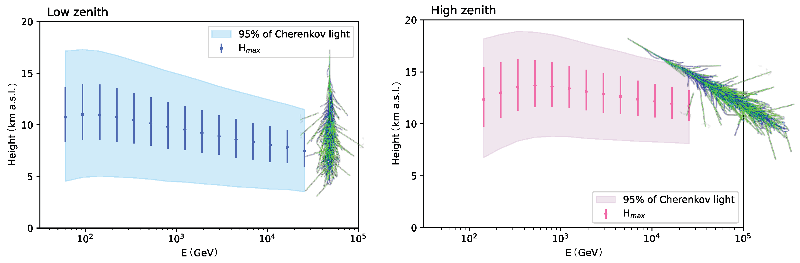
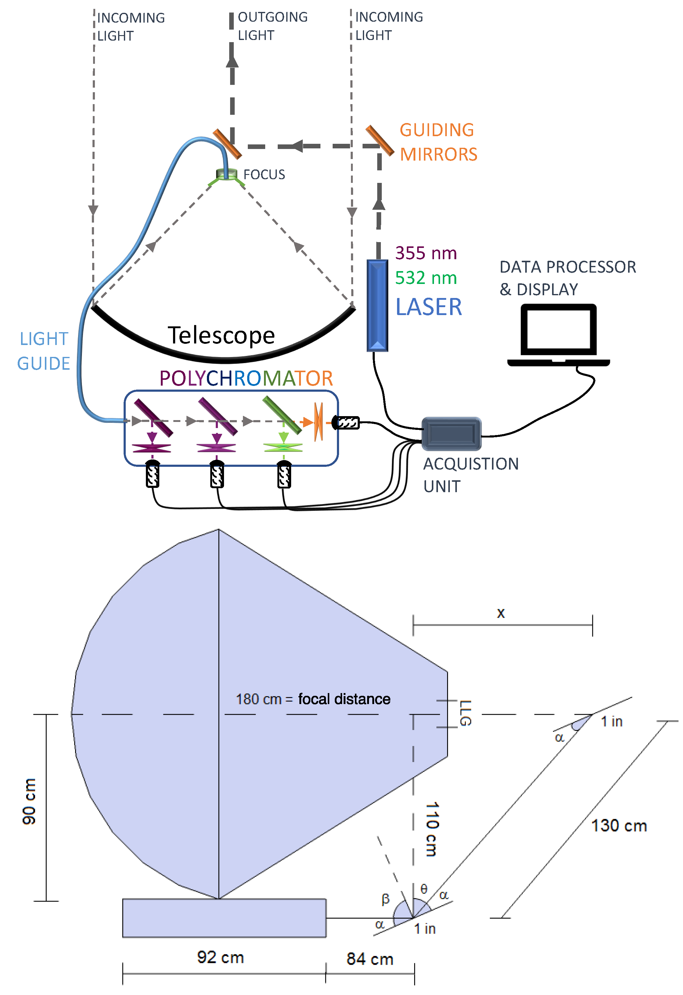
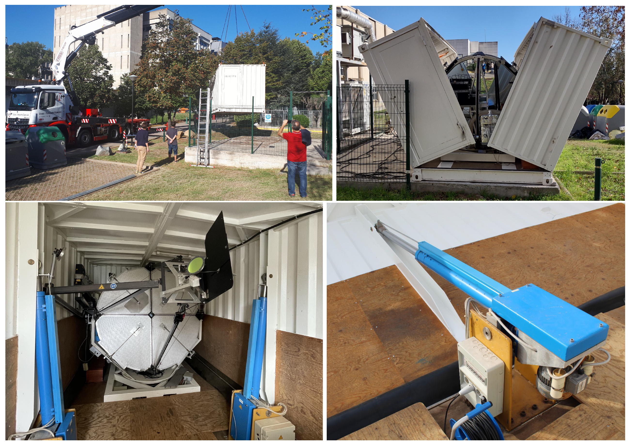
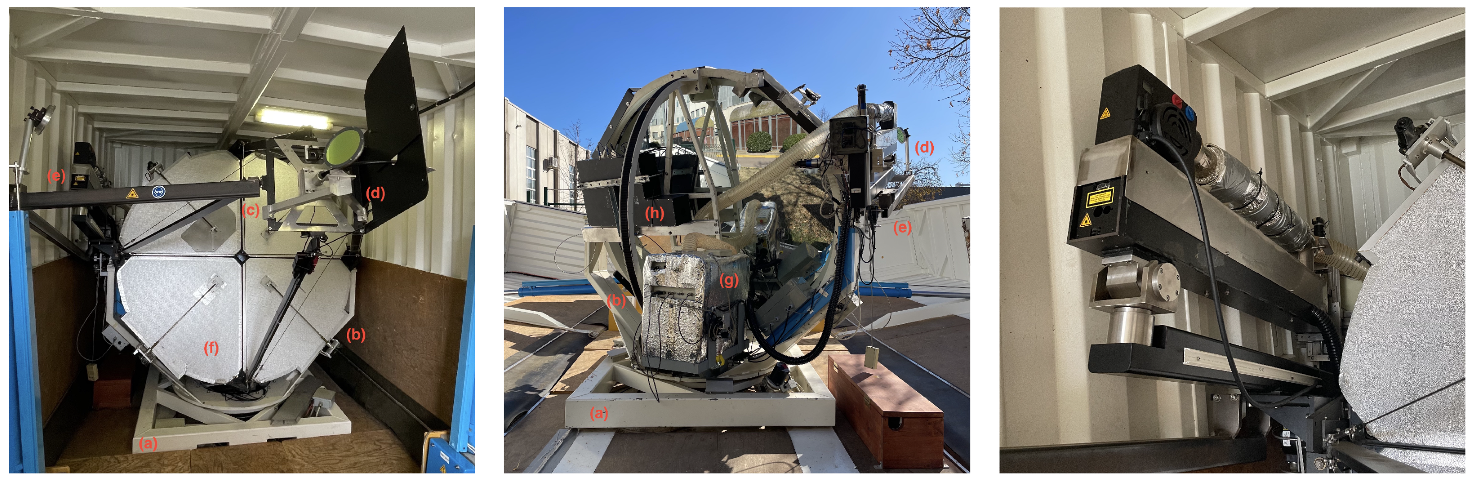
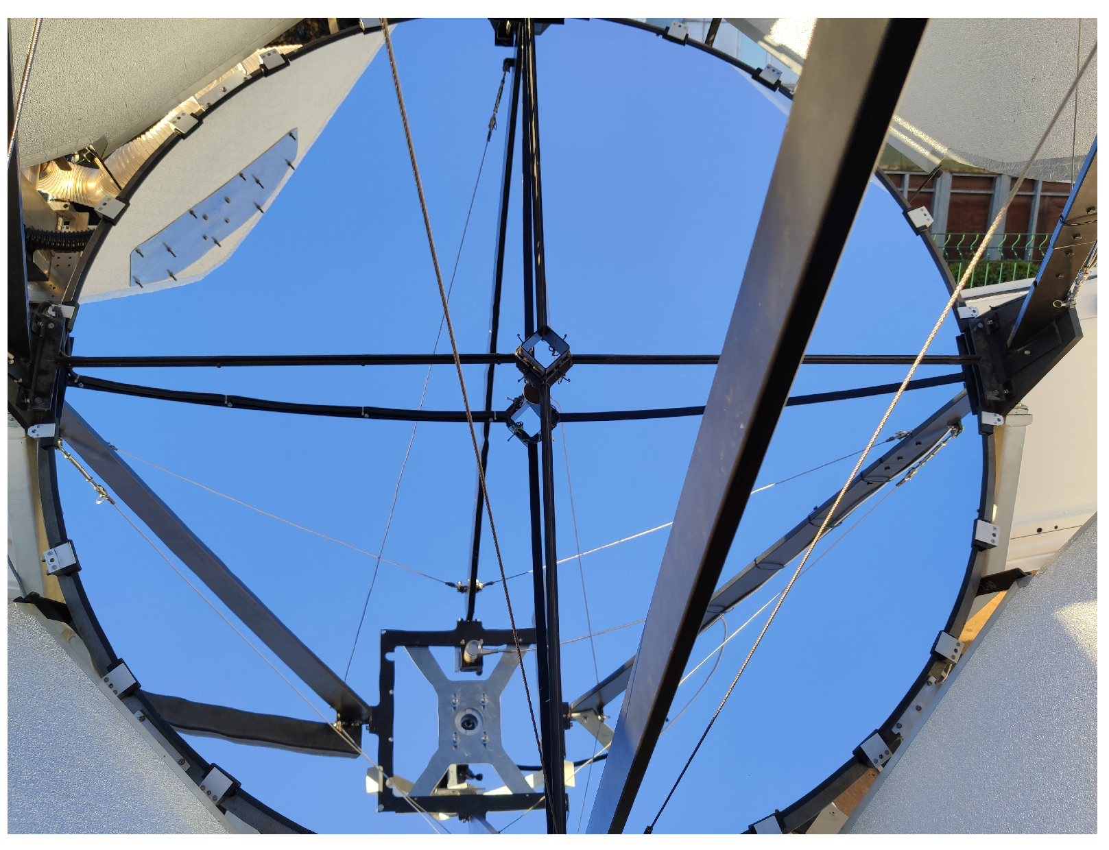
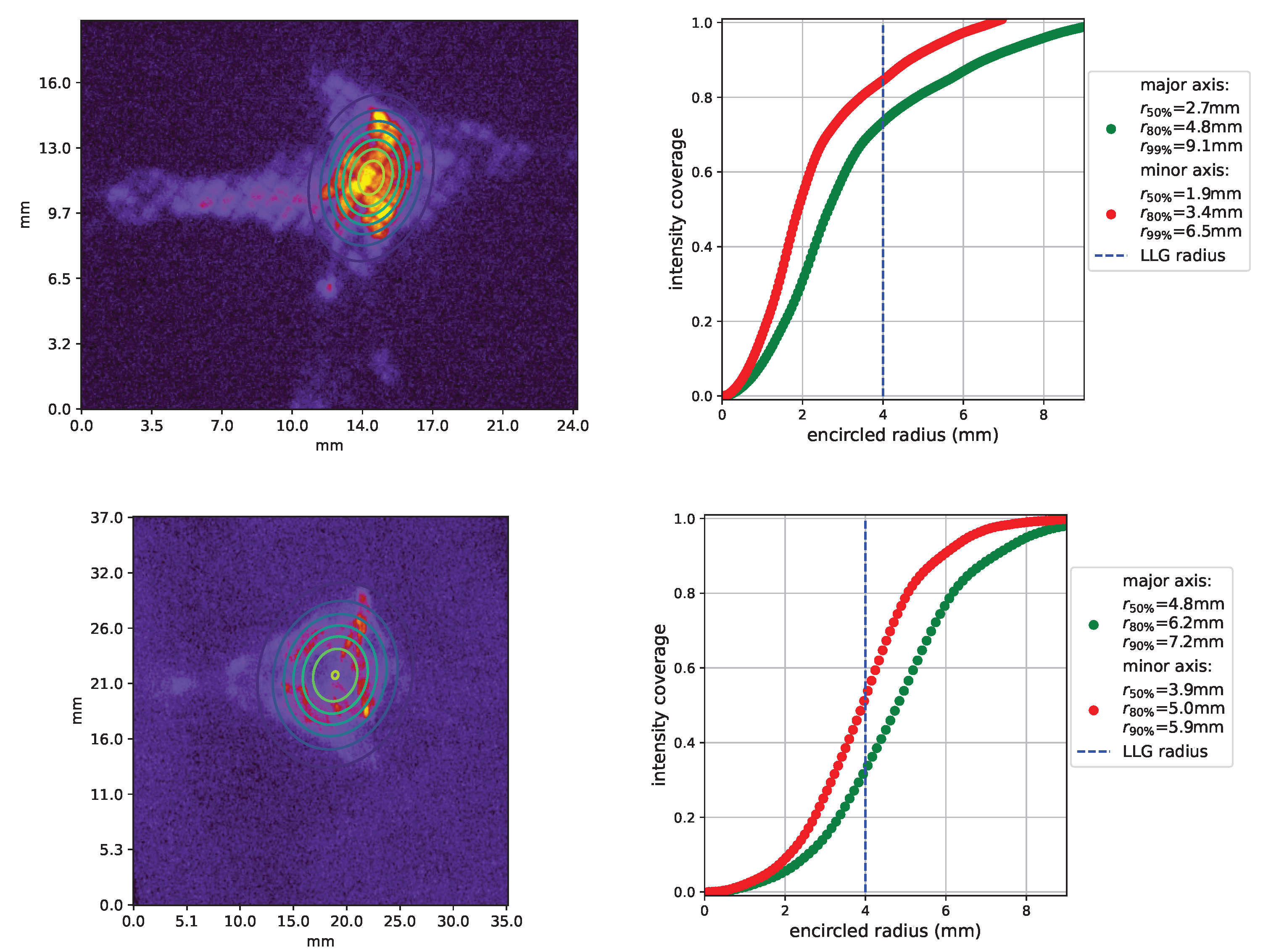

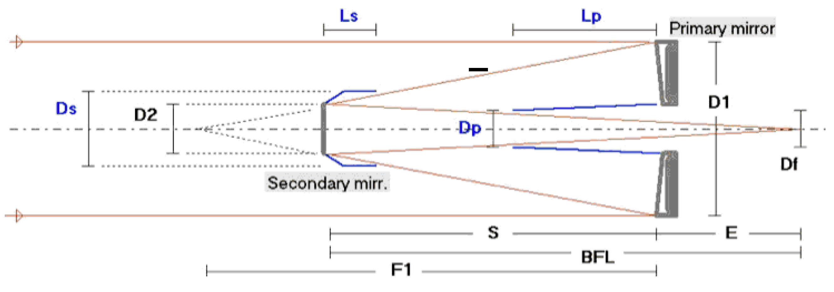
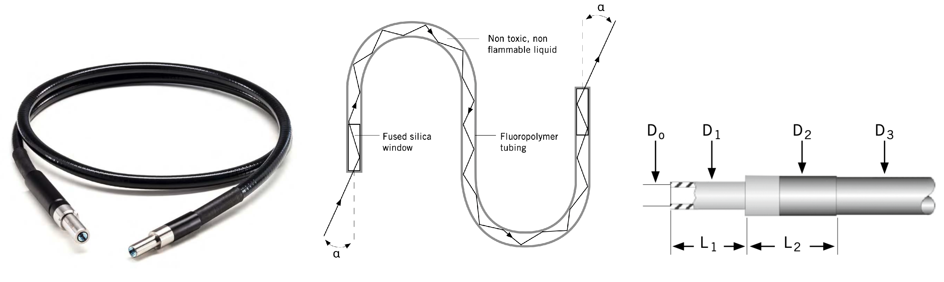

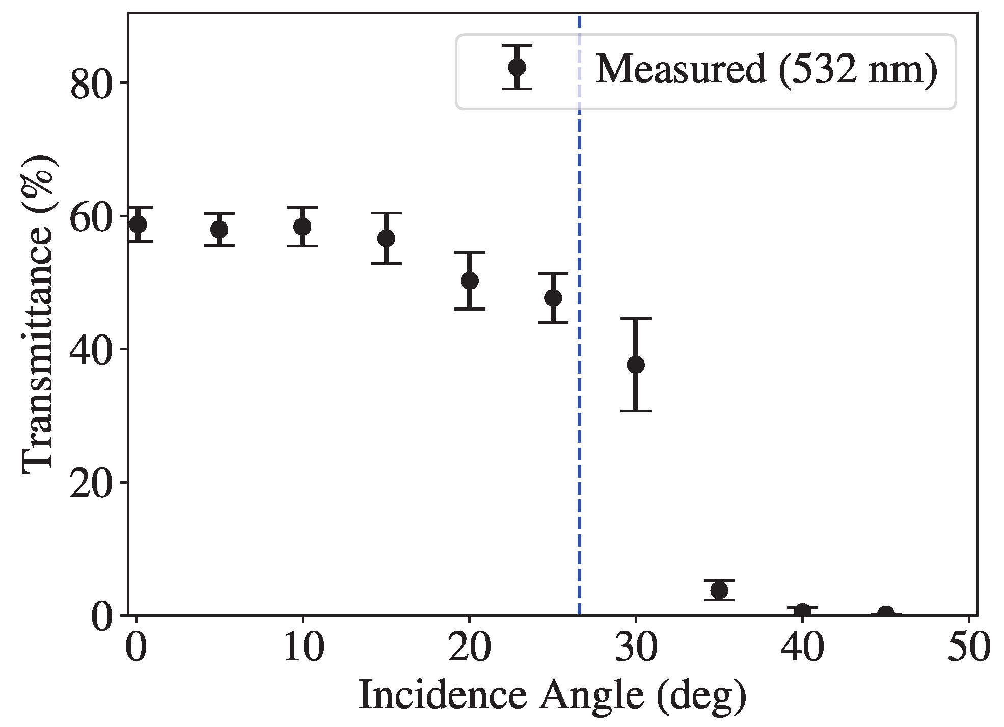
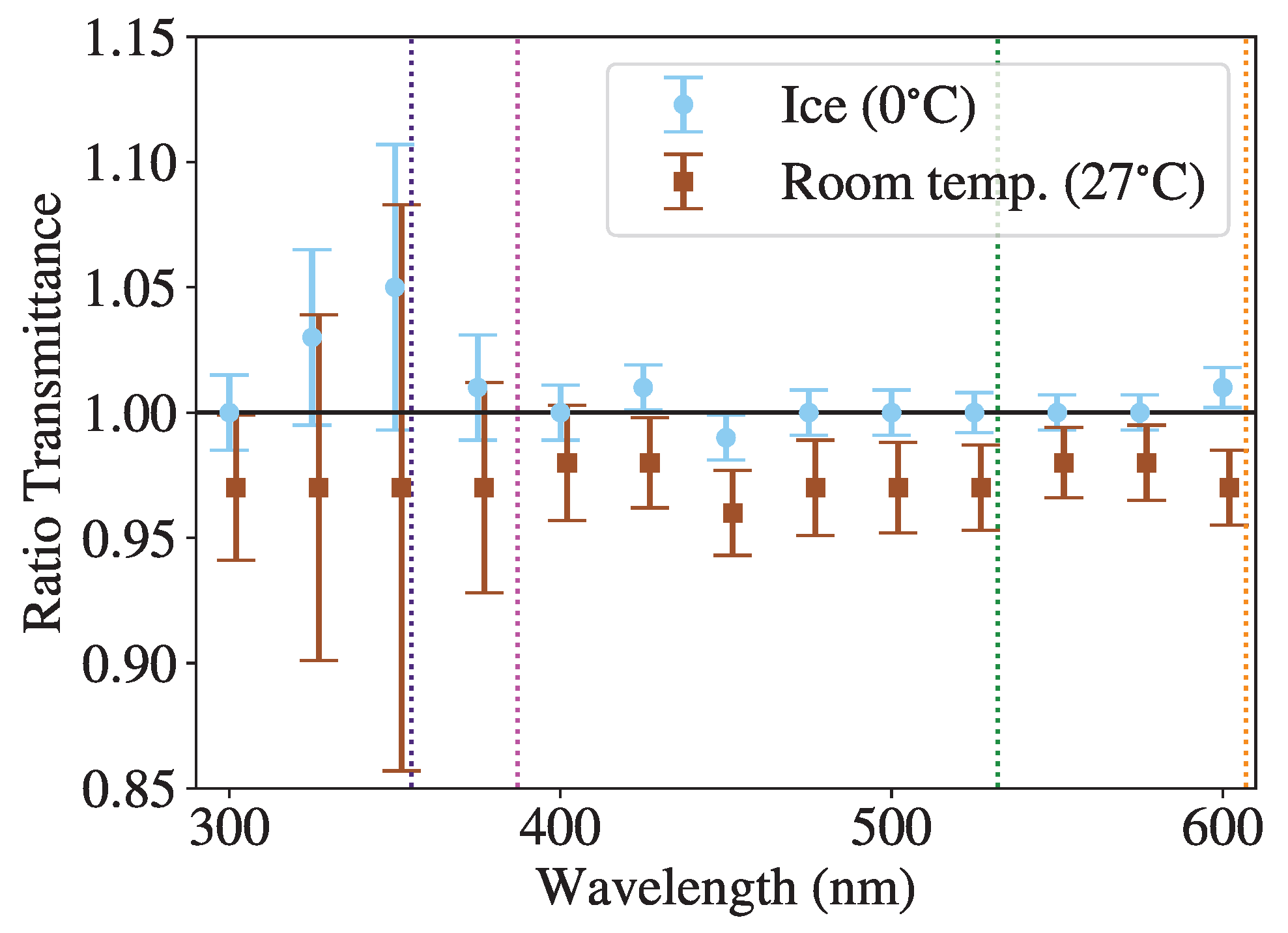

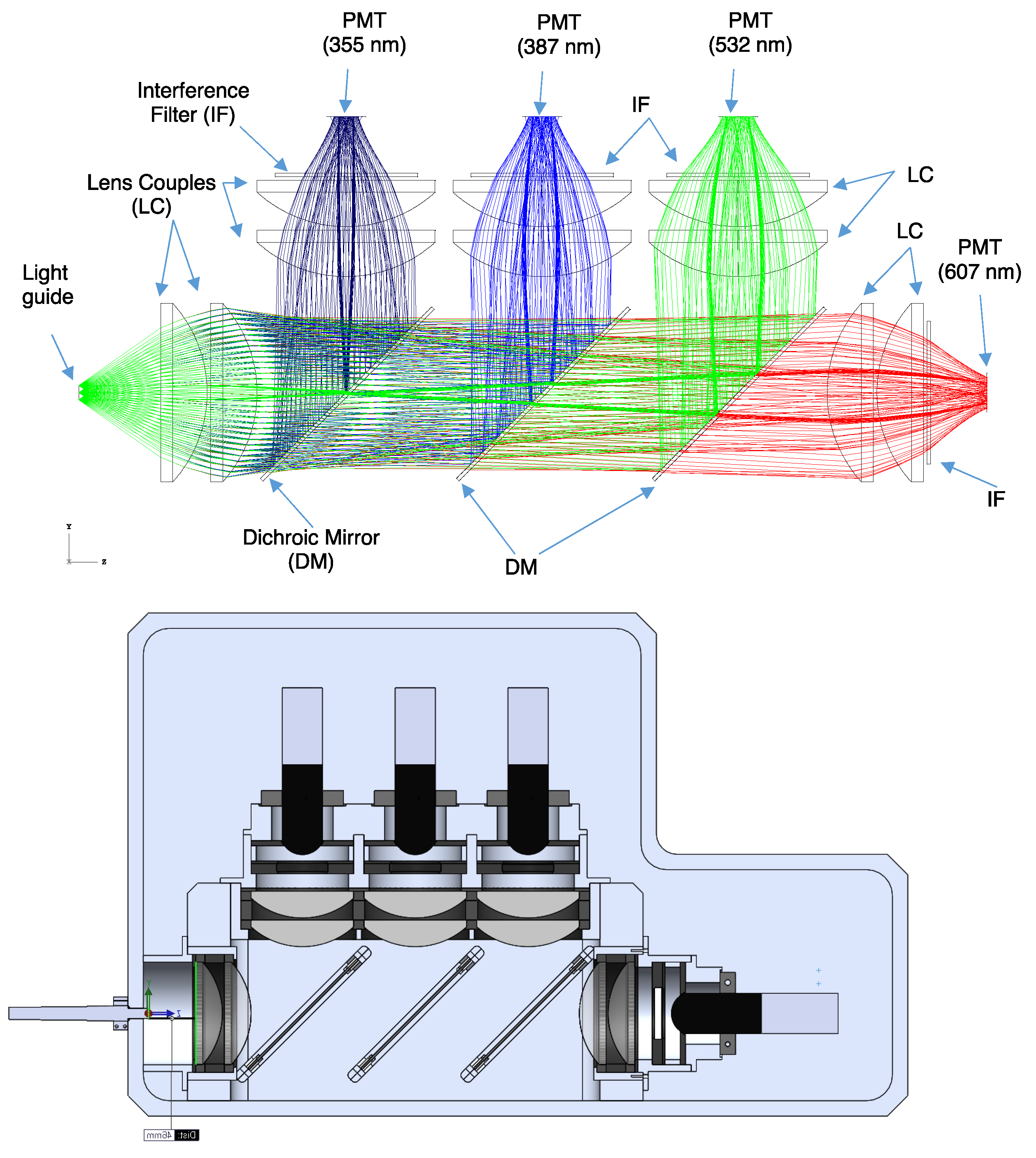
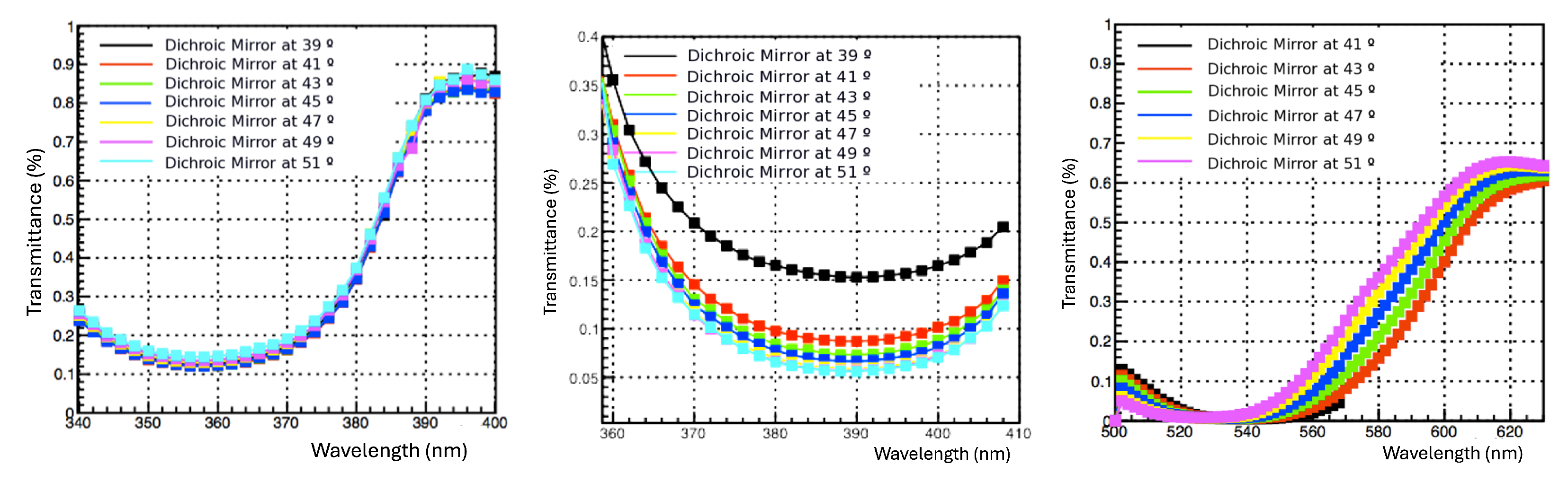
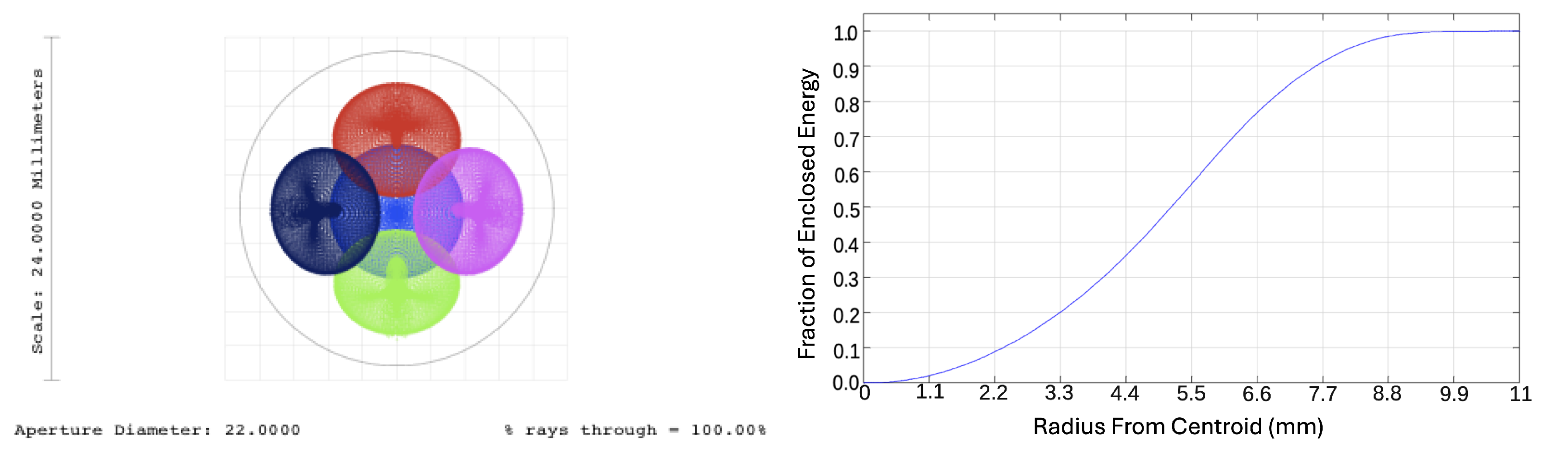
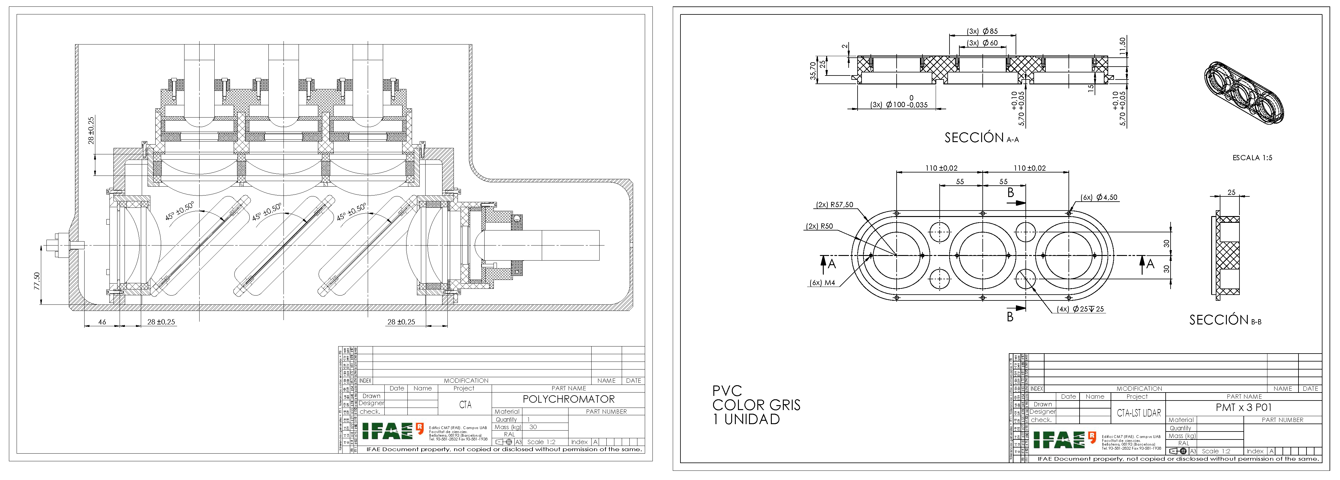
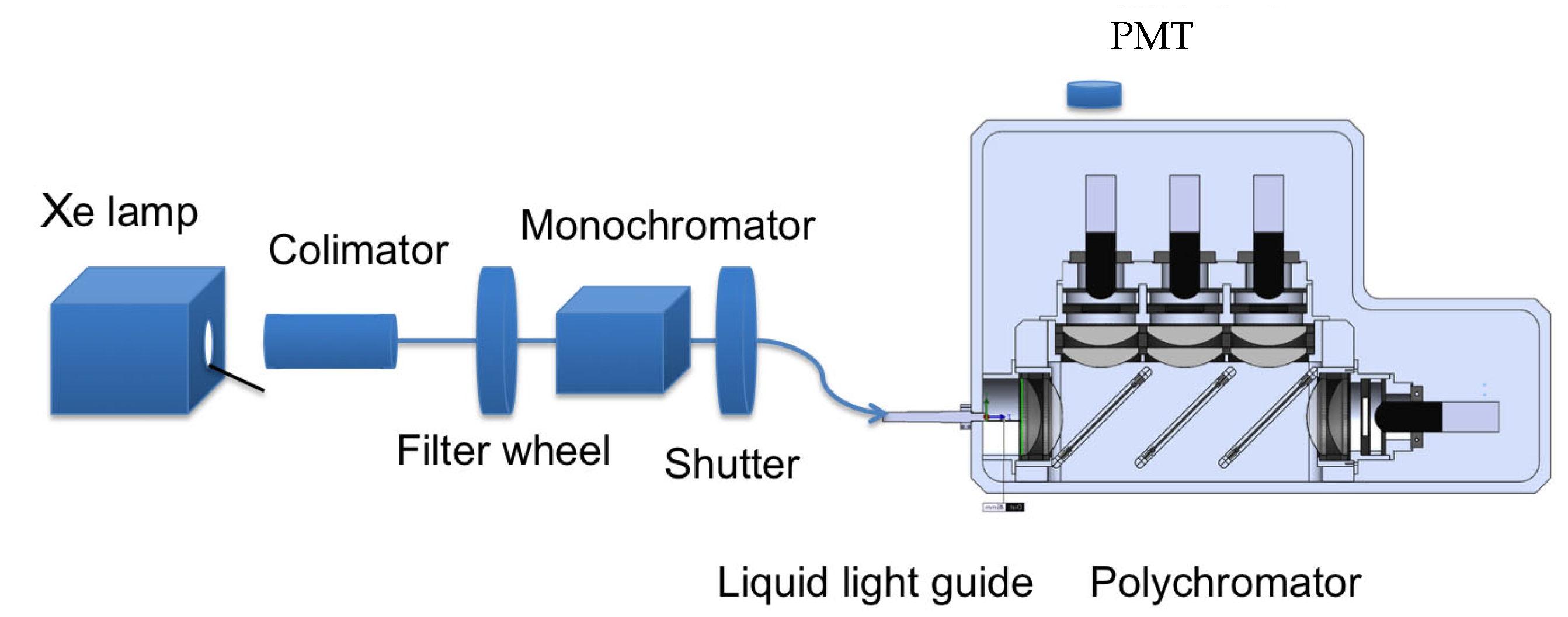
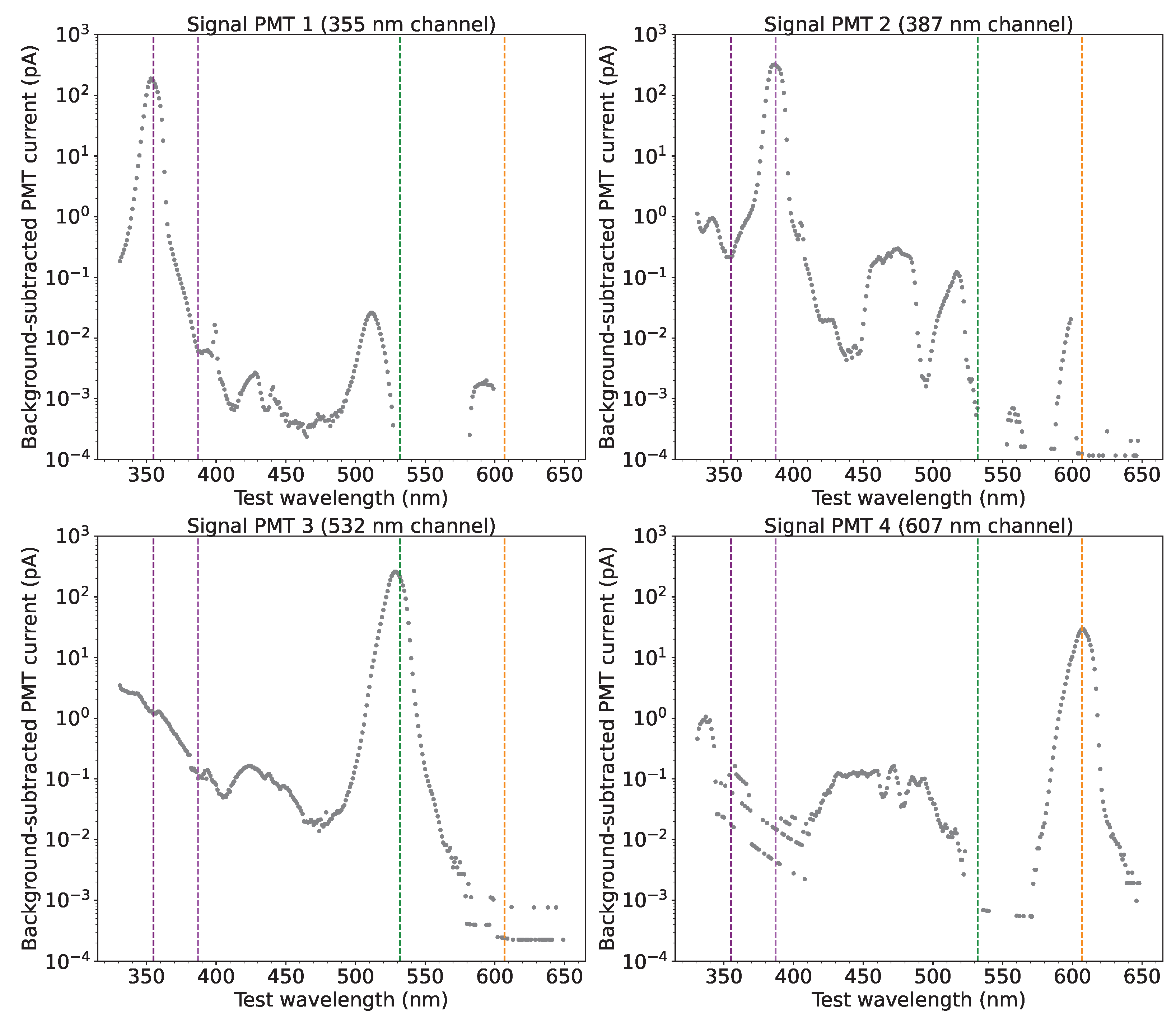
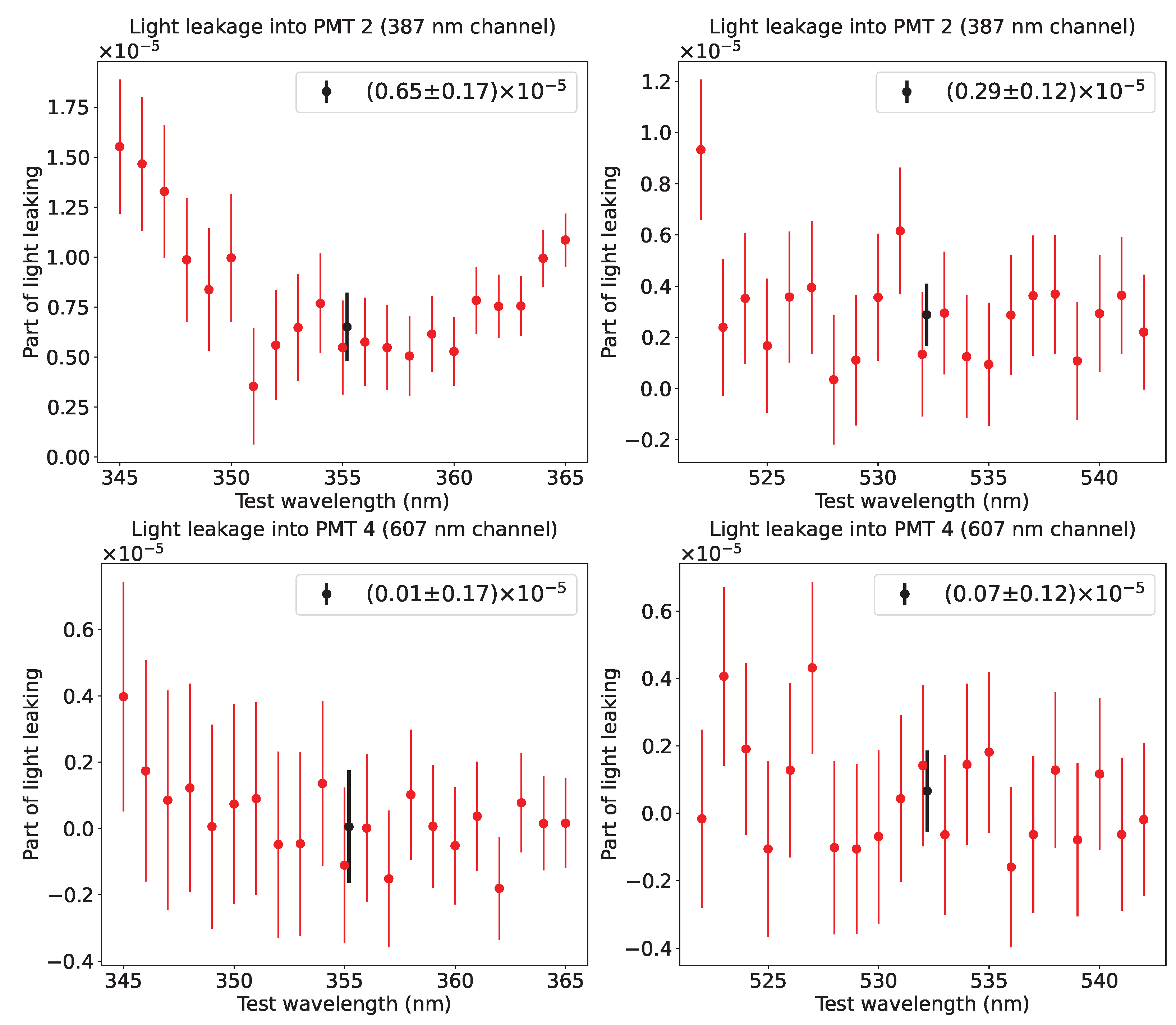
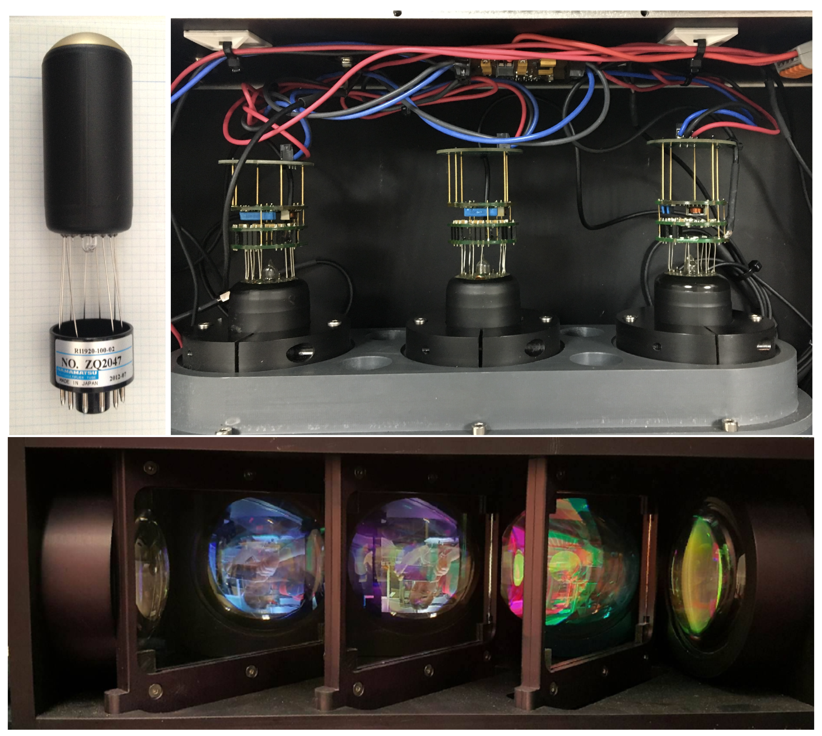
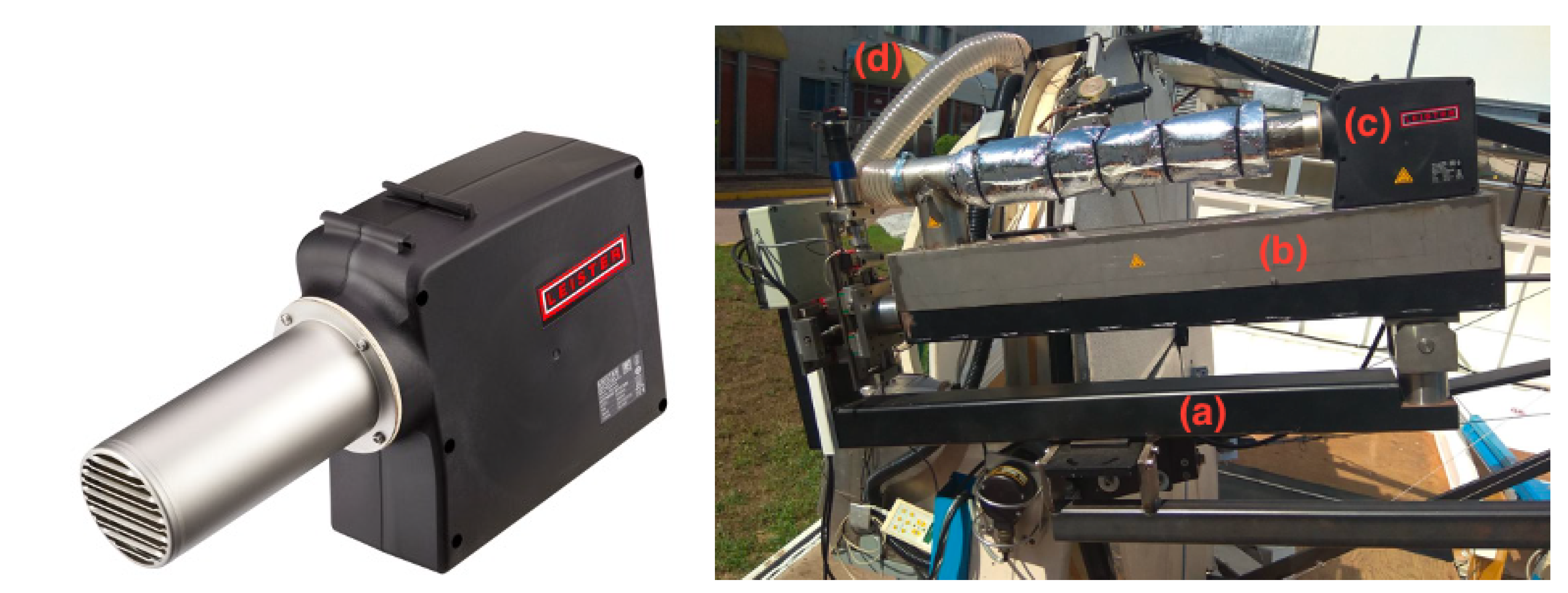
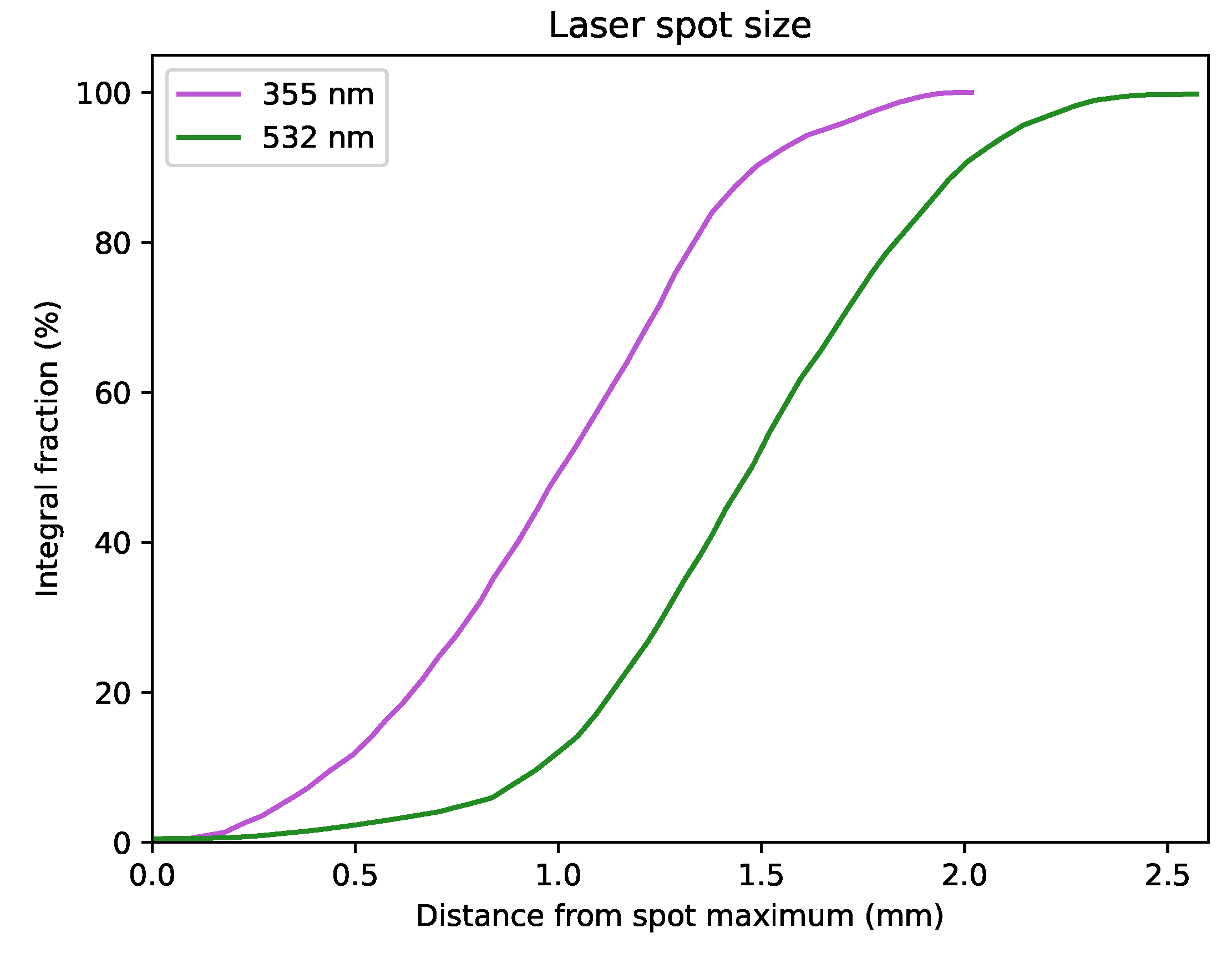

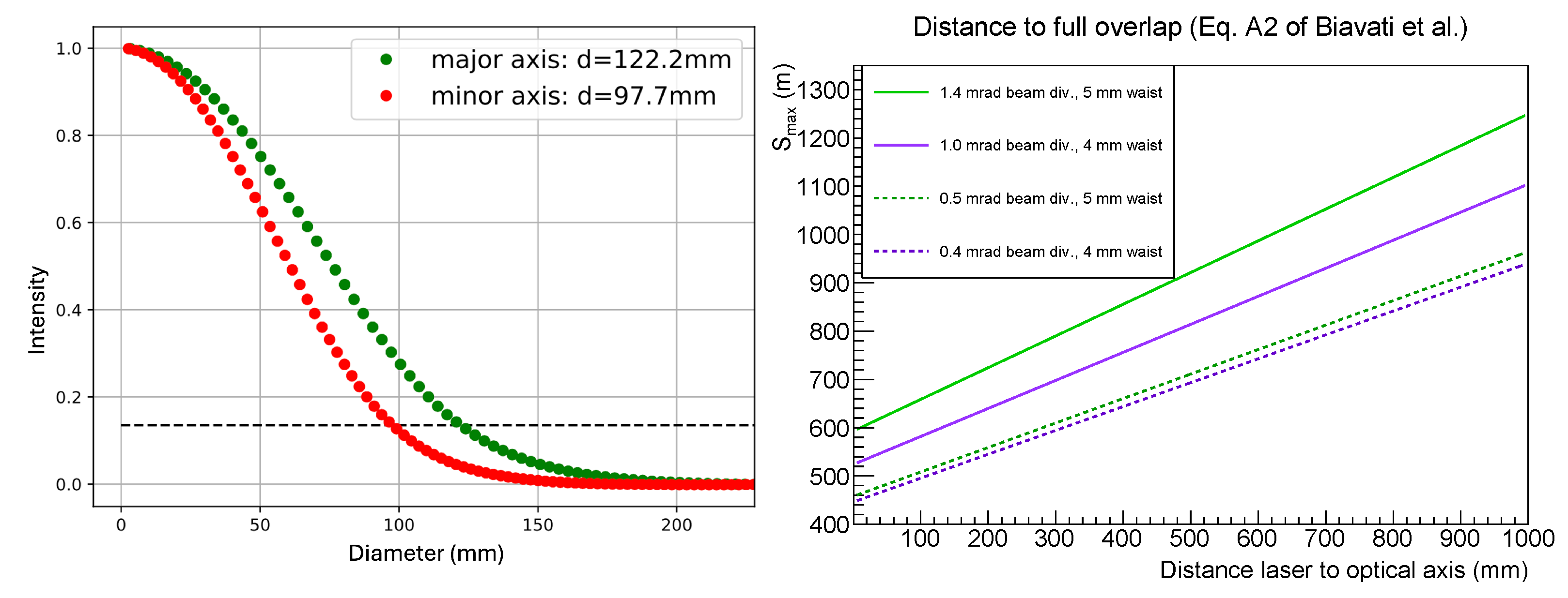


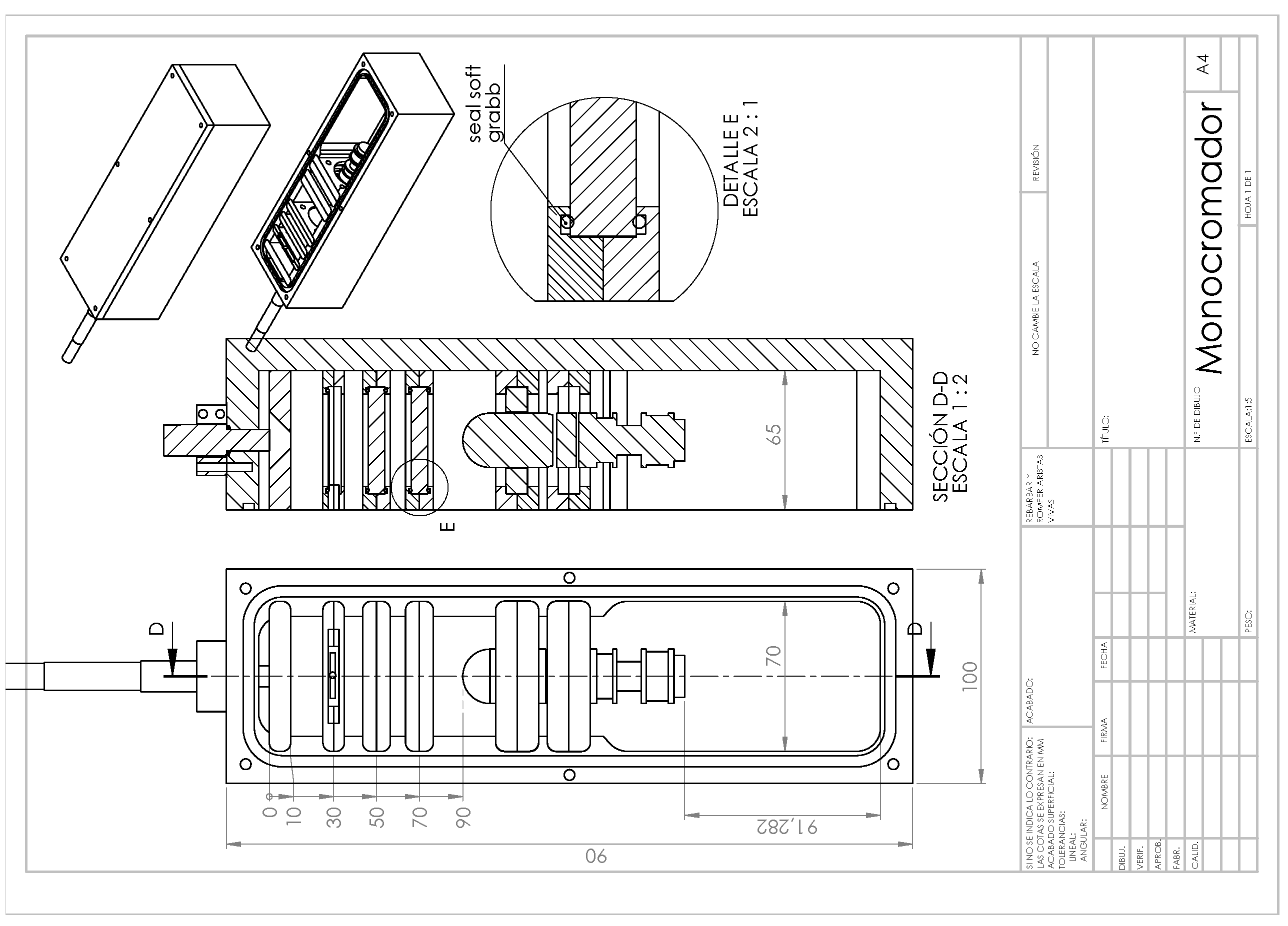
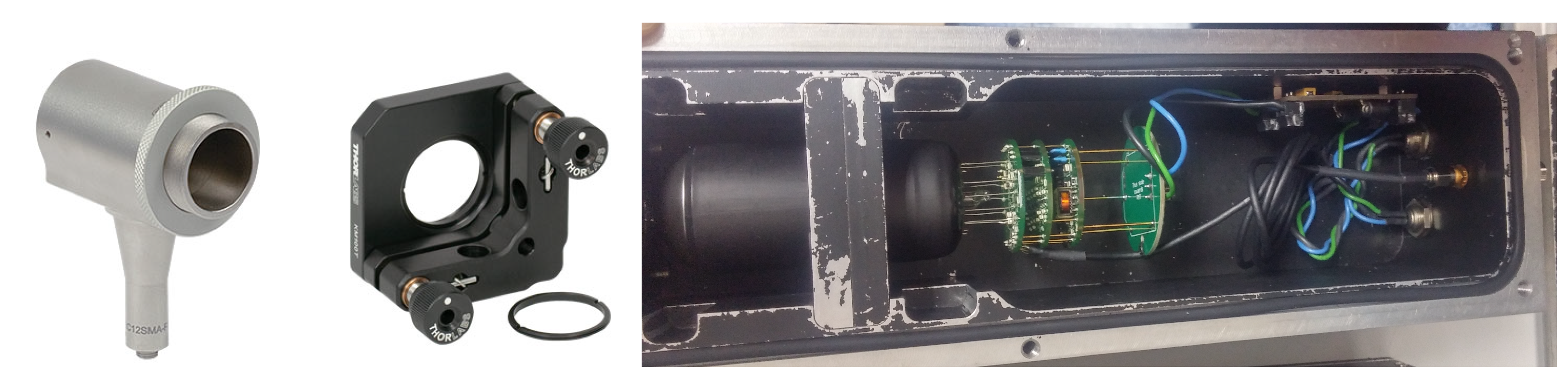
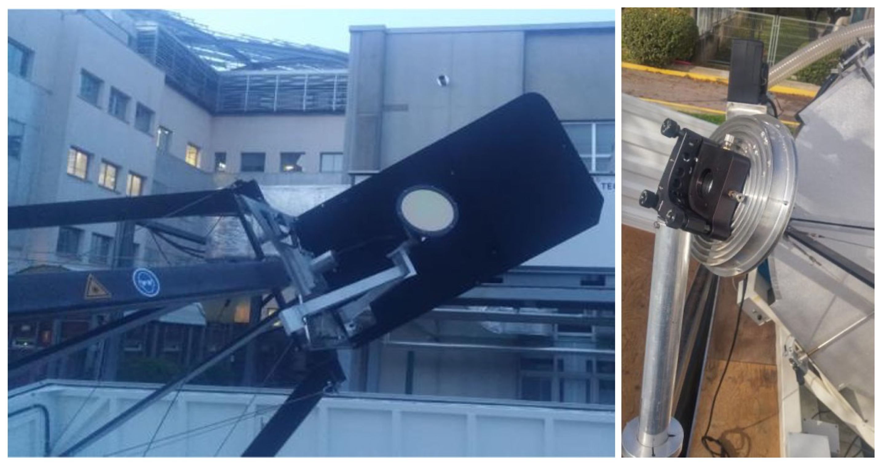
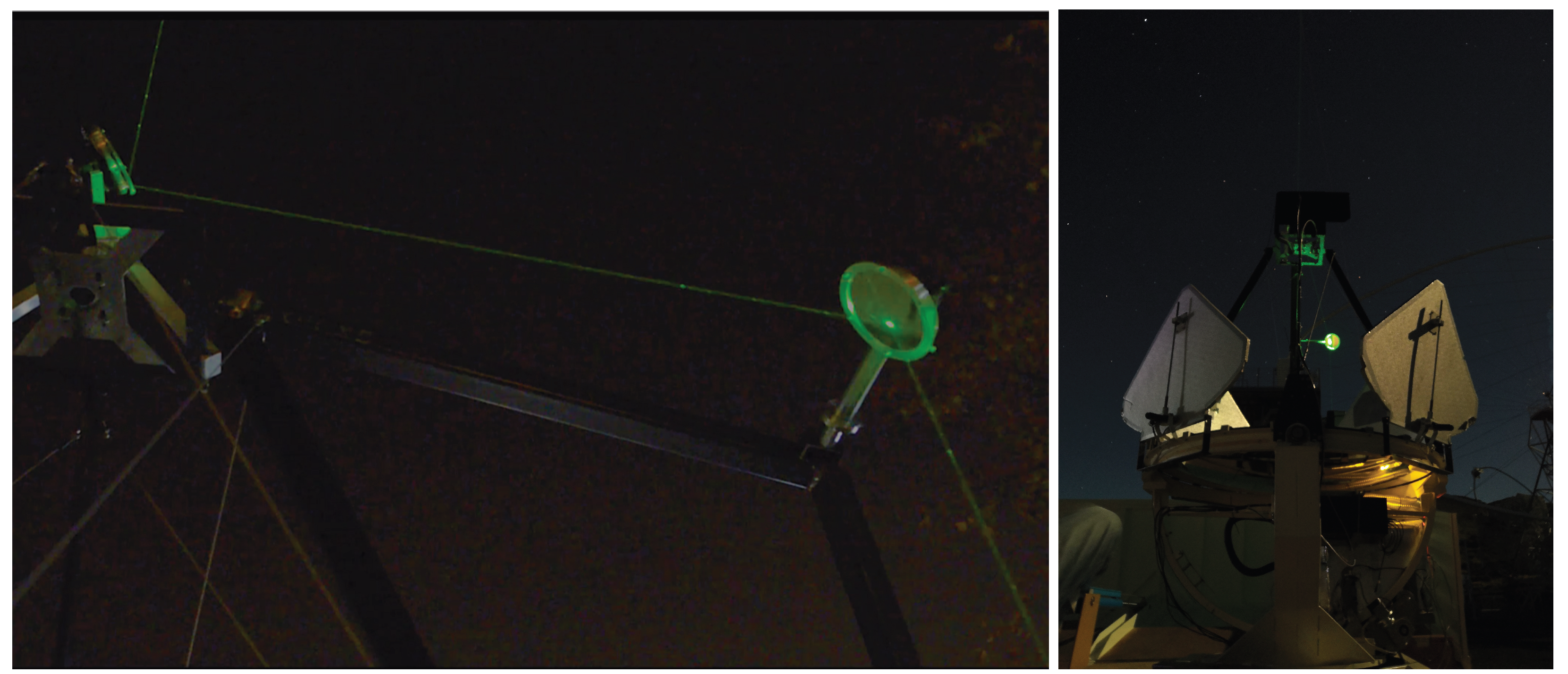
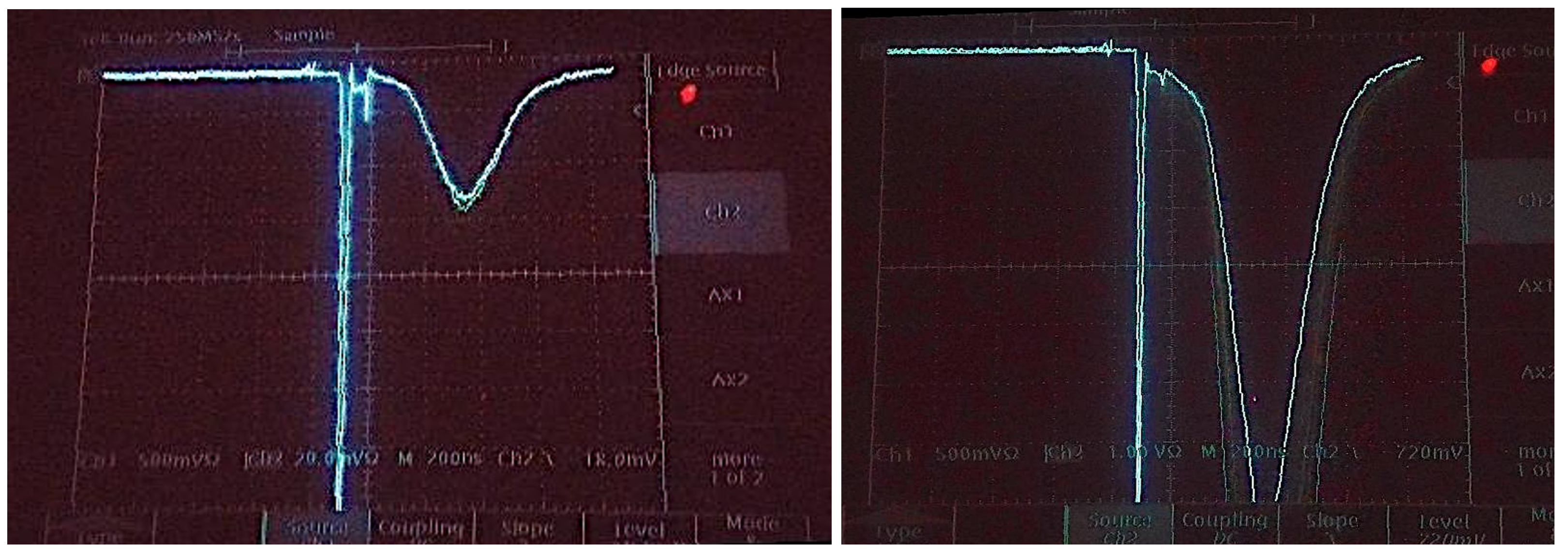
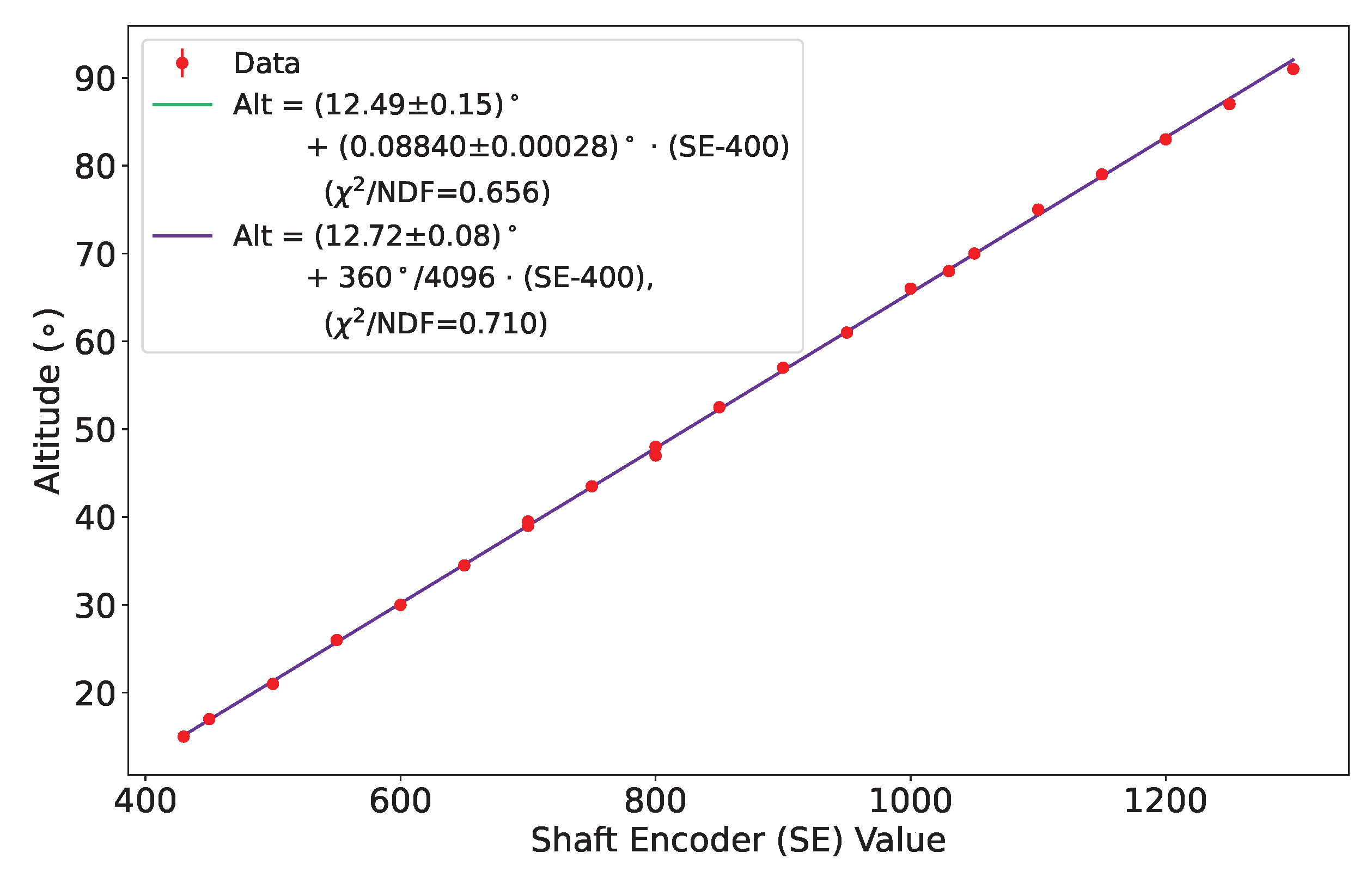

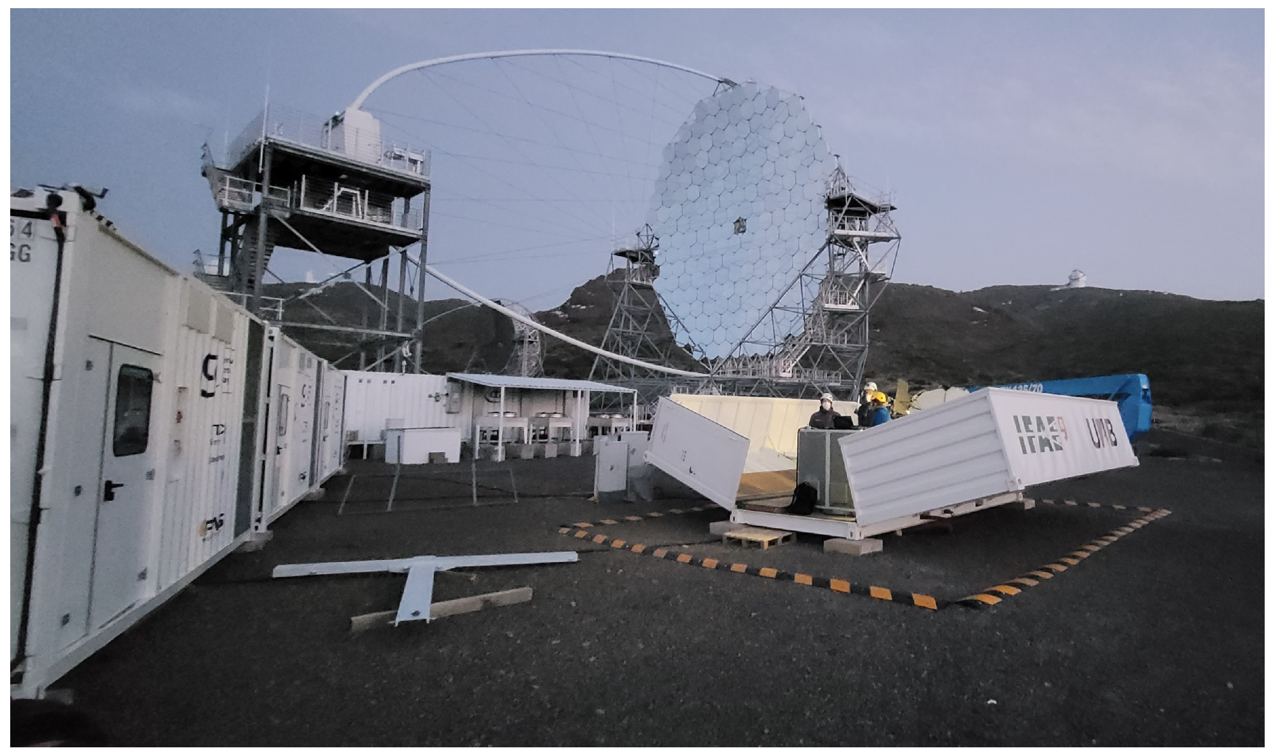
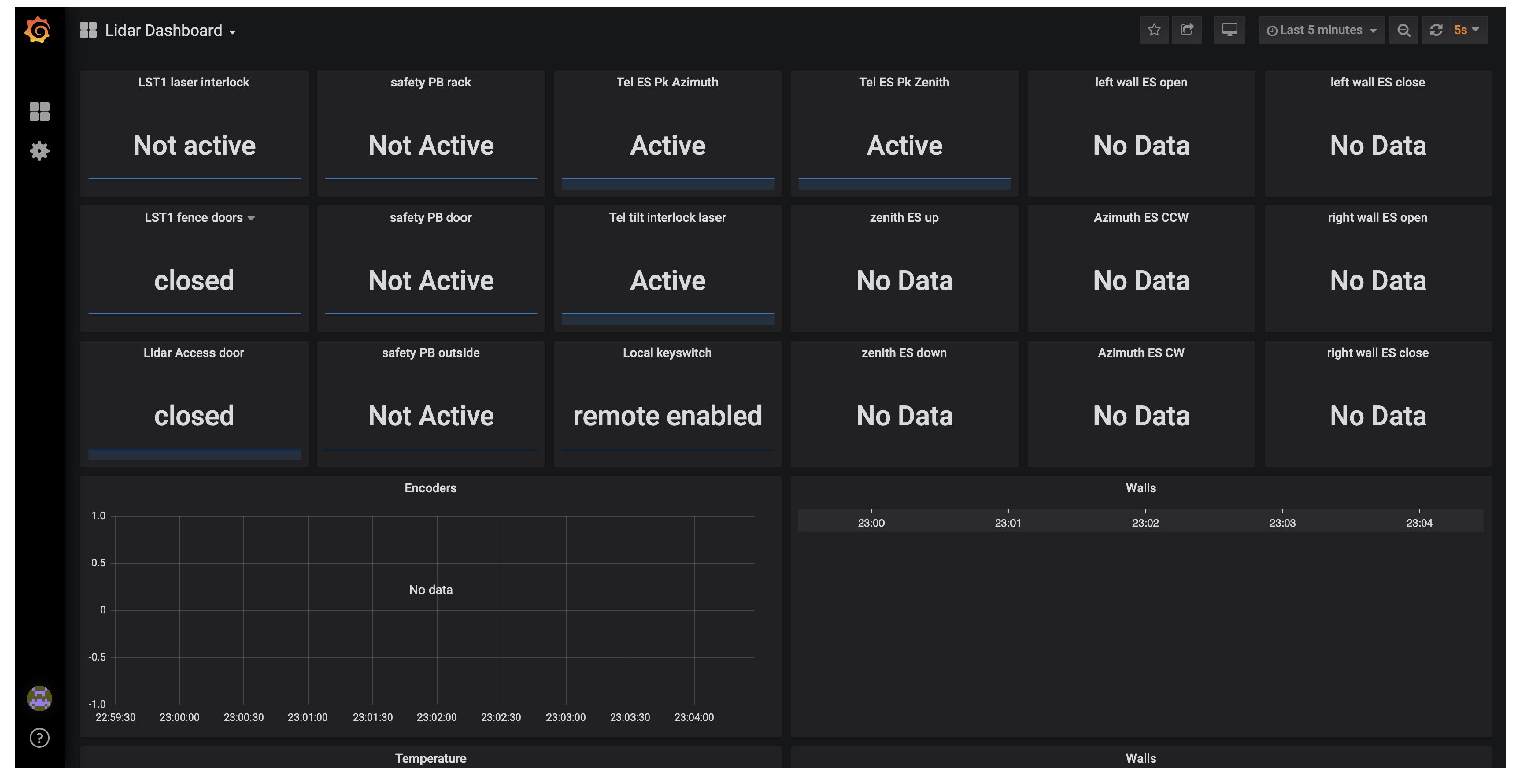
Disclaimer/Publisher’s Note: The statements, opinions and data contained in all publications are solely those of the individual author(s) and contributor(s) and not of MDPI and/or the editor(s). MDPI and/or the editor(s) disclaim responsibility for any injury to people or property resulting from any ideas, methods, instructions or products referred to in the content. |
© 2025 by the authors. Licensee MDPI, Basel, Switzerland. This article is an open access article distributed under the terms and conditions of the Creative Commons Attribution (CC BY) license (https://creativecommons.org/licenses/by/4.0/).