Abstract
The air temperature near the Earth’s surface is one of the most important meteorological and climatological parameters. Yet, accurate and timely readings are not available in significant parts of the world. The development and first validation of a methodology for the estimation of the near-surface air temperature (NSAT) is presented here. Machine learning and satellite products are at the core of the developed model. Land Surface Analysis Satellite Application Facility (LSA SAF) products related to Earth’s surface radiation, temperature and humidity budgets, albedo and land cover, along with static topography parameters and weather station measurements, are used in the analysis. A series of experiments showed that the Random Forest regression with 20 selected satellite and topography predictors was the optimum selection for the estimation of the NSAT. The mean absolute error (MAE) of the NSAT estimation model was 0.96 °C, while the mean biased error (MBE) was −0.01 °C and the R2 was 0.976. Limited seasonality was present in the efficiency of the model, while an increase in errors was noted during the first morning and afternoon hours. The topography influence in the model efficiency was rather limited. Cloud-free conditions were associated to only marginally smaller errors, supporting the applicability of the model under both cloud-free and cloudy conditions.
1. Introduction
The near-surface air temperature (hereafter, NSAT) is one of the most important meteorological parameters for forecasters and researchers. Its impact in every-day life and all kinds of socioeconomic activities cannot be overestimated. So, it is essential to have accurate and on-time readings of the near-surface air temperature at a high spatial resolution. Weather stations can provide such readings with a high level of accuracy; however, the dense spatial coverage of the Earth’s surface is, in many cases, difficult due to a variety of reasons. For example, extreme topographies could pose problems in the installation and correct operation of weather stations. In less-developed countries of the planet, the lack of funding often leads to significant deficiencies in the coverage.
Environmental satellites can offer information on the Earth’s surface and atmosphere. The plethora of available data have different characteristics, strong points and deficiencies. Satellites in geostationary orbits, like the European Meteosat series, present the advantage of continuous observation of their field of view. Their scanning frequency varies but, in general, it is in the order of minutes. Meteosat Second Generation (MSG), operated by EUMETSAT (the European Organisation for the Exploitation of Meteorological Satellites), was the primary meteorological geostationary satellite of Europe from 2004 to 2024. It scanned its field of view every 15 min, with a maximum horizontal resolution of 3 km in the infrared and 1 km in the visible spectrum (at the nadir subsatellite point).
During the last decades, substantial efforts were made in the subject of the estimation of the air temperature close to the Earth’s surface using satellite data as the primary input. For example, Stisen et al. [1] estimated the diurnal variation in the air temperature in parts of Africa using the Spinning Enhanced Visible and Infrared Imager (SEVIRI—onboard MSG satellites) data split-windows techniques and the Temperature Deviation Index Method (TVX) [2]. Amongst the other limitations of their approach, a cloud-free fraction of 90% within the window was necessary. The diurnal variation in the air temperature was based on an interpolation scheme using the time of day as the independent variable. A precision of about 3 °C and a bias of −1.1 °C was achieved. The parameterization of the air temperature through the combined use of SEVIRI and MODIS (Moderate Resolution Imaging Spectroradiometer) instruments was attempted by Zakšek and Schroedter-Homscheidt [3]. After a statistical downscaling of the SEVIRI data to a 1-km resolution, the 2-m air temperature over parts of Central Europe was estimated from the land surface temperature with an empirical parameterization, employing down-welling surface short-wave flux, relief characteristics and the NDVI. LSA SAF and NWC SAF (Support to Nowcasting and Very Short Range Forecasting) data were used as the satellite input, except for the NDVI, which was derived from MODIS measurements. Their analysis resulted in an RMSD of 2.00 °C, a bias of 0.01 °C and a correlation coefficient of 0.95. Only cloud-free pixels were considered.
The TVX empirical algorithm for the air temperature estimation was calibrated and validated over the Iberian Peninsula by Nieto et al. [4]. They used SEVIRI data and applied the TVX algorithm only if two-thirds of the pixels were classified as non-cloudy. Their results showed an MAE of 2.8 °C, an RMSE of 3.7 °C and an overestimation of 1.0 °C when analyzing the hourly dataset. The daily maximum air temperature was adequately approximated with an RMSE of 5 °C. Shen and Leptoukh [5] estimated the surface air temperature over central and eastern Eurasia from the MODIS land surface temperature using a linear regression method. Only clear-sky days were considered for the computation of the MODIS surface temperature. It was argued that the relationships between the maximum Ta and daytime Ts depended significantly on the land cover, but the relationships between the minimum Ta and night-time Ts were weakly dependent on the land cover. Therefore, different linear regression equations of the maximum Ta estimation were calculated for the several land cover groups, while, for the minimum Ta, no distinction between land cover groups was made. The mean absolute error of the maximum Ta was found to range between 2.4 °C and 3.2 °C, while, for the minimum Ta, the MAE was about 3.0 °C. Hengl et al. [6], using MODIS LST, topographical, time and insolation data, employed principal component analysis-formulated models of the estimation of daily air temperature maps over Croatia. They achieved an average accuracy of ±2.4 °C. Parmentier et al. [7] assessed a collection of methods and remote sensing-derived covariates for regional predictions of the 1 km daily maximum air temperature. Mean elevation, MODIS LST and distance to the ocean were amongst the most frequently significant covariates besides the latitude and longitude, which were included by default in the models. Using the top set of covariates, it was found that the MAE ranged from 1.93 °C to 2.02 °C between the three interpolation methods, while the ME was negative and did not exceed −0.11 °C. Stepwise regression analysis was employed by Janatian et al. [8] in order to simulate the average air temperature at daily and weekly scales over Iran. A series of predictors, including MODIS LST, were examined for their importance in the formulation of the temperature. The proposed model estimated the average Tair with a mean absolute error of 2.3 °C and 1.8 °C at daily and weekly scales, respectively. Only cloud-free pixels were considered. Hooker et al. [9] constructed a global dataset of air temperature at a 0.05 ° horizontal resolution using MODIS LST monthly data and a statistical model that incorporated information on geographic and climatic similarity. The RMSE ranged from 1.14 °C to 1.55 °C. Historical minimum, maximum and average air temperature models at 1 km and 200 m resolution over France were constructed by Hough et al. [10] using linear mixed models with MODIS and Landsat data in combination with spatial predictors. According to their validation, the MAE ranged from 0.9 °C to 1.4 °C for the 1 km dataset. Nascetti et al. [11] employed a neural network regression model to estimate the maximum air temperature in Puglia, Italy, using NDVI and LST Landsat-8 data. Pixels with cloud cover over 50% were excluded. They managed to reach an R2 of 0.8, suggesting a quite successful fit.
Overall, most of these methods managed to calculate the desired temperature parameters (instantaneous, daily, mean, maximum, minimum, monthly mean, etc.) with an acceptable degree of accuracy. However, these methods operate under non-cloudy conditions, while most of them are not adequate for the continuous real-time estimation of the air temperature. The use of a semi-predefined daily curve of air temperature is another shortcoming in some of those methodologies, as it limits the margin for strong short-term temperature variations during, e.g., short periods of cloudiness or rain. Finally, some of these methods use relationships that are strongly dependent on region, and therefore they are not suitable for use in other areas.
In this paper, we present our research on the subject of the continuous, near-real-time estimation of the NSAT under both cloudy and non-cloudy conditions. LSA SAF products and static topographic parameters are used for the estimation of the NSAT. The LSA SAF products are computed using land surface energy balance approximations and models [12], and they are representative of the surface temperature, the radiation and heat fluxes at the Earth’s surface, the evapotranspiration and the land cover and albedo. Since the land surface energy balance, the turbulent heat fluxes, the radiation fluxes, the dynamics inside the boundary layer, the land surface temperature and the NSAT are strongly linked [13,14,15,16], the selected LSA SAF products are considered ideal to be included in a model that attempts to estimate the NSAT.
One of the main novel features of our approach is the ability to estimate the NSAT under both cloudy and non-cloudy conditions using the all-sky-enabled products of Meteosat satellites, something that is accomplished for the first time over the European continent, according to the authors’ knowledge. As stated earlier, there were several attempts to estimate the air temperature, with very good results; however, all of them were limited to non-cloudy periods. Such an innate deficiency renders them non-applicable during cloudy conditions, which are obviously frequent during adverse weather. Our method, using Meteosat products that are available under cloudy and non-cloudy conditions, overcomes the problem and performs under all kinds of weather. A second, quite important novel element is the ability of the easy and fast near-real-time estimation of the NSAT, provided that the necessary data are available in near-real-time.
The NSAT can be used in nowcasting operations as an extra source of information, and by authorities and policy makers in facing and quickly adapting to challenges related to extreme heat or frost. Provided that the necessary LSA SAF data are available, the NSAT could be applied to create archives of NSAT datasets. Such archives could be employed in research studies that require reliable near-surface air temperature data in areas where weather station coverage is poor, or in cases where a homogenous dataset is required.
Finally, as most of the input data are derived from geostationary satellite products and freely accessible topography parameters, our method can easily offer continuous temperature information over regions where weather stations are sparse or absent. Such a strong potential for operational application makes our method a valuable source of weather data for every-day operational activities.
2. Data and Methodology
2.1. Data
Three primary sources of data were utilized in the present analysis. Static topographic parameters and LSA SAF products were employed as predictors of the near-surface air temperature, while temperature data, derived from the network of surface weather stations operated by the METEO Unit at the National Observatory of Athens (METEO/NOA), acted as the ground truth for the training and validation of the models. Their draft description follows.
2.1.1. LSA SAF Satellite-Derived Data
As stated on EUMETSAT’s website [17], Satellite Application Facilities (SAFs) are dedicated centers of excellence for processing satellite data. The EUMETSAT Secretariat supervises and coordinates the activities of the SAF network, ensuring that the SAFs in operation are providing reliable and timely operational services related to meteorological and environmental issues. The LSA SAF [18] uses satellite observations to create a series of products focused on agriculture, forestry, land-use planning and disaster management.
Archived LSA SAF products for the 2-year period from July 2020 to June 2022 were used for the training and validation of our models. Each of them is available in the MSG projection, with an approximate horizontal resolution of 5 Km (over Greece). All of the products were used as they provided by the LSA SAF, and no adjustments were made to them. These parameters, along with their maximum temporal resolution and their abbreviations, are presented in Table 1. The sub-daily parameters were used at a 30 min temporal resolution, while, for the 4 daily parameters, their daily value was assigned to all 30 min values of the respective day. Total (TOT), Diffuse (DIF) and Direct (DIR) parts were extracted and analyzed from the Total and Diffuse Downward Surface Shortwave Flux (SSF) product. The Broadband Shortwave Bi-Hemispherical (BB-BH), Shortwave Directional-Hemispherical (BB-DH), Near-Infrared Directional–Hemispherical (NI-DH) and Visible Directional–Hemispherical (VI-DH) parameters were extracted and analyzed from the AL product. The 30 min differences were also computed and analyzed for the SSF, LF, LE, H and ET parameters (the full names of the Land SAF products are given in Table 1). It should be noted here that the radiation and heat fluxes and the evapotranspiration parameters refer to the ground surface, and therefore are considered relevant to the formulation of the NSAT. Finally, the great advantage of the LSA SAF products used here is that they are computed for both cloudy and non-cloudy conditions. More about these products can be found on the LSA SAF website [18].

Table 1.
Land SAF products, along with their maximum temporal resolution and their acronym.
To account for the period (noon, midnight, sunrise, etc.) of the day and, more specifically, the sun illumination conditions, the sun zenith angle (SZA) of each pixel scan was also included in the analysis. The SZA is a better indicator of the period of the day, as it is irrelevant of the time zone and the distance of a site to the prime meridian. These data were kindly provided by the LSA SAF after request.
2.1.2. Static Topographic Parameters
Static topographic data computed from the Geodata.gov.gr shapefiles [19], the Copernicus eu-dem-v1.1-25m downloaded from the Copernicus website [20] and, finally, location information of the weather stations were used for the training and validation of the models (more information follows later in this section). Table 2 presents these parameters, along with their source, units and a very brief description.
Table 2.
Static topographic parameters, along with their source, units and description.
2.1.3. Weather Stations Observed Temperatures
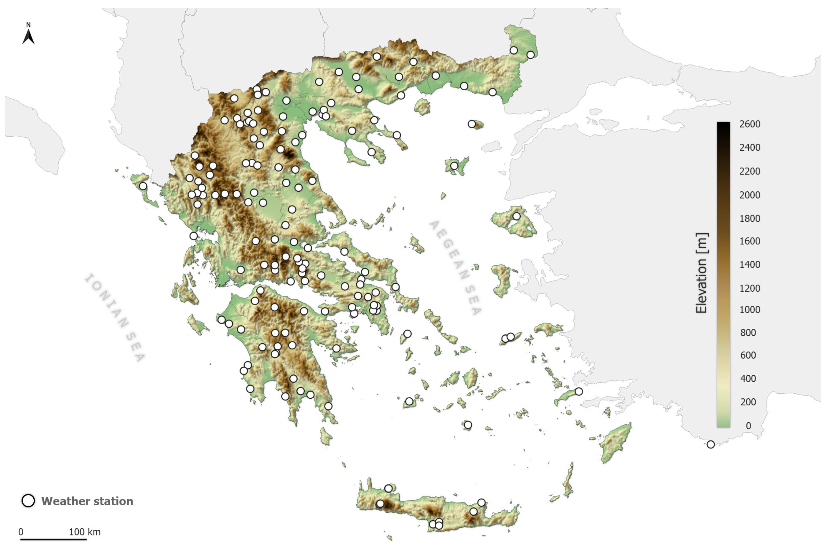
Τemperature data were extracted from the archive of the METEO/NOA weather station network data archive [21]. A total of 126 stations distributed over the Greek mainland and islands were used. Temperature was archived every 10 min. The offset between the nominal time of the scan of the MSG and the actual scan time of the Greek area approached 10 min. Following that, the HH:00 and HH:30 images actually scanned the Greek area around HH:10 and HH:40, respectively. Therefore, the HH:10 and HH:40 temperature records were selected as the corresponding ground truth. Figure 1 shows the station locations overlaid on the topography of the area.
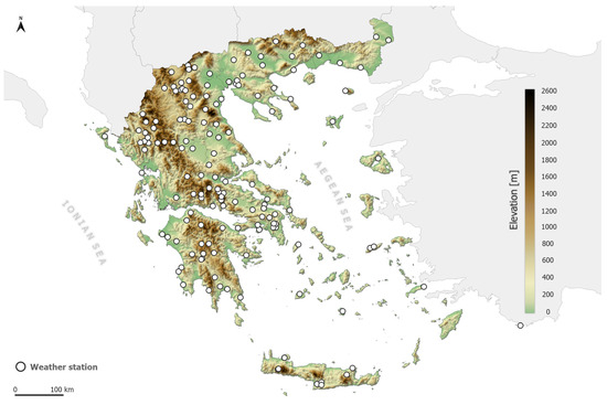
Figure 1.
Locations of the 126 weather stations of the METEO/NOA network overlaid on the Greek topography.
2.2. Methodology
The following three machine learning methods were employed to create the NSAT estimation models: Random Forest (RF), Extreme Gradient Boosting (XGBoost) and Artificial Neural Networks (ANNs). These three methods were selected after a literature review, which showed that they are amongst the most commonly used in model development in Earth sciences research (e.g., [22,23,24,25]). The models were trained using the Keras and scikit-learn libraries of the Python v3.7 scripting language.
2.2.1. Random Forest
Random Forest is a machine learning method that combines multiple decision trees to improve the accuracy in classification and regression tasks [22]. Each tree is built independently, and predictions are made by averaging the outputs for regression or using majority voting for classification. This approach is particularly useful for handling large weather datasets [26]. The main parameter to adjust is the number of trees [23]. In this study, the Random Forest Regressor was configured as follows:
- n_estimators: 60;
- min_samples_split: 2;
- min_samples_leaf: 2;
- random_state: 42.
2.2.2. Extreme Gradient Boosting
XGBoost is an optimized implementation of the Gradient Boosting method, designed for efficiency and scalability [27]. Unlike Random Forest, which trains trees independently, XGBoost builds trees sequentially, with each new tree correcting the residual errors of the previous ones. This iterative process improves the prediction accuracy for both regression and classification tasks. The algorithm also includes regularization techniques to prevent overfitting, making it widely used in research and high-performance applications [24]. In this study, the XGBoost Regressor was configured as follows:
- n_estimators: 500;
- max_depth: 5;
- learning_rate: 0.1;
- random_state: 42.
2.2.3. Artificial Neural Networks (ANNs)
Artificial Neural Networks (ANNs) are computational models inspired by the human brain, commonly used for predicting meteorological parameters [25]. This study employed a Multilayer Perceptron (MLP), a type of feedforward ANN widely applied in air temperature prediction [28,29]. An MLP consists of interconnected neurons organized into an input layer, one or more hidden layers and an output layer, where each neuron processes weighted inputs through an activation function [30].
For this study, a deep feedforward neural network was implemented with six hidden layers, progressively reducing from 1000 to 50 neurons, with each using ReLU activation. The output layer consisted of a single neuron with a linear activation function for continuous predictions. The model was trained using the Adam optimizer with the mean squared error (MSE) as the loss function and the mean absolute error (MAE) as an evaluation metric. To prevent overfitting, early stopping was applied, halting the training if validation loss did not improve for 50 epochs. The model was trained for up to 15 epochs with a batch size of 50.
The dataset was divided into the following two parts: the training subset and the validation subset. The first one was used for the training of the models, while the second one was used for the efficiency testing of the developed models. The validation subset consisted of 20% of the total predictors/ground truth pairs. One of every five consecutive (in terms of time) sets of values was set aside for the validation procedures. In simple words, one set of values every 2.5 h was reserved for the validation dataset. In that way, we avoided any known physical cycles, thus making the training and the validation subset unbiased from any daily, monthly or annual cycles. All of the training and validation in our analysis (namely, the training and validation for the selection of the model and number of predictors, plus the training and validation of the selected model) used these two datasets. Finally, the bin analyses metrics were computed using the validation subset.
A series of frequently used error metrics were computed to assess the degree of efficiency of each model.
Mean Biased Error:
Mean Absolute Error:
Root Mean Square Error:
where is the estimation of the algorithms, is the temperature observations, N is the total number of estimation–observation pairs and is the average value of the observations. More information about the statistics used can be found on the WWRP/WGNE Joint Working Group on Forecast Verification Research webpage [31].
The coefficient of determination , which expresses the proportion of the variation in the dependent variable that is predictable from the independent variables, was computed and examined. The best possible score was 1.0, while it could also acquire negative values. The negative values occurred when the model fit the data worse than the worst possible least-squares predictor. A constant model that always predicts the average value of the predictand would obtain an of 0.0. The coefficient of determination was computed according to the following formula:
where .
All of the metrics, in all cases, were computed using the validation dataset.
Each method and model had a set of hyperparameters that needed to be initialized. To objectively select the initial values of the hyperparameters, we used the GridSearchCV method (an exhaustive search over specified parameter values for an estimator). This approach involved conducting multiple test scenarios with various combinations of hyperparameter values and evaluating the accuracy achieved in each case. By running 20 iterations and providing the hyperparameters of each method as inputs, we determined the optimal settings.
A high number of predictors results in higher computation costs, complicated and non-robust models and the requirement of large amounts of input data. So, the final selection and tuning of the hyperparameters were based on the results of these tests and combinations, taking into account both the performance and the computational efficiency of each model during training.
In most models, only a small subset of the feature parameters contributes significantly to the overall variability of the target parameter. A ‘feature importance’ is calculated for each predictor of the RF, XGBoost and ANN (the sum of weights for the ANN), which effectively represents the weight that each predictor carries in determining the estimated parameter. Therefore, it is logical to reduce the number of predictors by discarding those with lower importance. However, selecting a feature importance threshold can be subjective and arbitrary. To address this, we opted for a more objective selection procedure.
Initially, all of the models ran using the full set of predictors, extracting, at the same time, the feature importance of each predictor. Then, for each of the models, multiple runs were performed, adding, in consecutive steps, the predictors one-by-one, starting from those with higher importance. The success metrics were recomputed in every step. Adding predictors was expected to improve, in general, the metrics, and the goal was to identify a number of predictors beyond which the metrics presented only minor changes. At the same time, the most efficient model was selected for the rest of the analysis.
It is important to examine how our model behaves in relation to topography and time in order to identify possible deficiencies, and maybe to advise caution when using it in such cases. All of the topography parameters, presented in Table 2, were split in 8 bins (including a similar number of stations), and then the MAE and MBE were computed for each of the bins. To identify the seasonal and sub-daily changes, the MAE and MBE were computed on a seasonal and hourly basis.
Finally, the efficiency of our model was examined under cloudy and non-cloudy conditions. The validation dataset was split in two parts. The first one comprised the cloud-free cases, while the second included all fully or partially cloudy pixels. The MAE and MBE were computed and analyzed for the two parts.
Summarizing the NSAT estimation model development procedure (Figure 2), it is comprised of 4 distinct steps. In step 1, the machine learning methods were selected and their basic parameters were tuned, while, in step 2, the classification of the available predictors in order of importance was made for each the three methods. Step 3 comprised two parallel parts. Each of the models was run again, adding predictors one-by-one in descending order of importance, aiming (a) to identify the most efficient model and (b) to identify the number of predictors that ensured accurate estimation and, at the same time, the reduction in the computational time and input data. Finally, step 4 examined the model efficiency under different topography, temporal and cloudiness conditions.
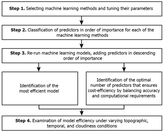
Figure 2.
Technical flow diagram of the NSAT estimation model development procedure.
3. Results
As stated in the Data and Methodology section, our first goal was to select the most efficient method and, at the same time, the most important features/predictors that will be included in that model. Additionally, our approach to model configuration during training aimed to minimize the computational cost and reduce the size of the exported model files. Following that, all of the models run with all available predictors and the ‘feature importance’ of each predictor were extracted.
Next, each of the selected models was re-run by adding, in consecutive steps, the predictors, starting from those with the higher importance. The success metrics were recomputed in every step. Figure 3 presents the graphs of the MAE vs. predictor rank for the Random Forest (RF), XGBoost (XGB) and Artificial Neural Networks (ANNs). The RF seemed to be the most efficient model, with an MAE that was smaller than XGBoost and the ANN after the introduction of the seventh predictor. It reached values below 1 °C with the introduction of the 16th predictor and, after that point, the MAE continued to drop at clearly lower rates. So, an acceptable threshold selection could be anywhere after the 16th or even the 7th predictor. However, it is noted that the MAE reached a value of 0.96 °C with the introduction of the 20th predictor and, after that, the MAE fluctuations were negligible. Introducing more predictors did not improve the model. We argue that the Random Forest (RF) with 20 predictors is the most accurate and cost-efficient one with respect to the accuracy of the estimations, the reduction in the computational time and the limitation of input data requirements. Therefore, the RF was selected for the development of the NSAT estimation model. All of the analyses and statistics that follow refer to that model.
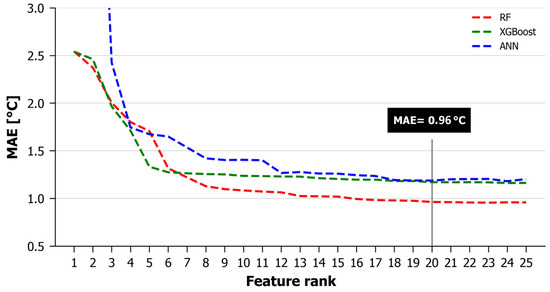
Figure 3.
MAE vs. predictor rank for the 3 models.
Regarding the rest of the metrics, the and RMSE presented similar behavior. The MBE showed continuous fluctuations of small amplitudes (smaller than 0.01 °C) for the RF and XGBoost, while the ANN had a clearly higher MBE (on the order of 1 °C). The related figures are not presented, as they do not offer more insights or information worth mentioning in the analysis.
The 20 predictors that were used in the Random Forest model are presented in Table 3 in descending order of importance. As deduced from the inspection of the Feature Importance column of the predictors, LST-AS dominates the formulation of the NSAT, while H, SLF and Cma follow, with values one order of magnitude smaller. The rest of the features present an importance two orders of magnitude smaller than LST-AS; therefore, their influence is rather limited.
Table 3.
Feature importance of the 20 predictors ingested in the RF model.
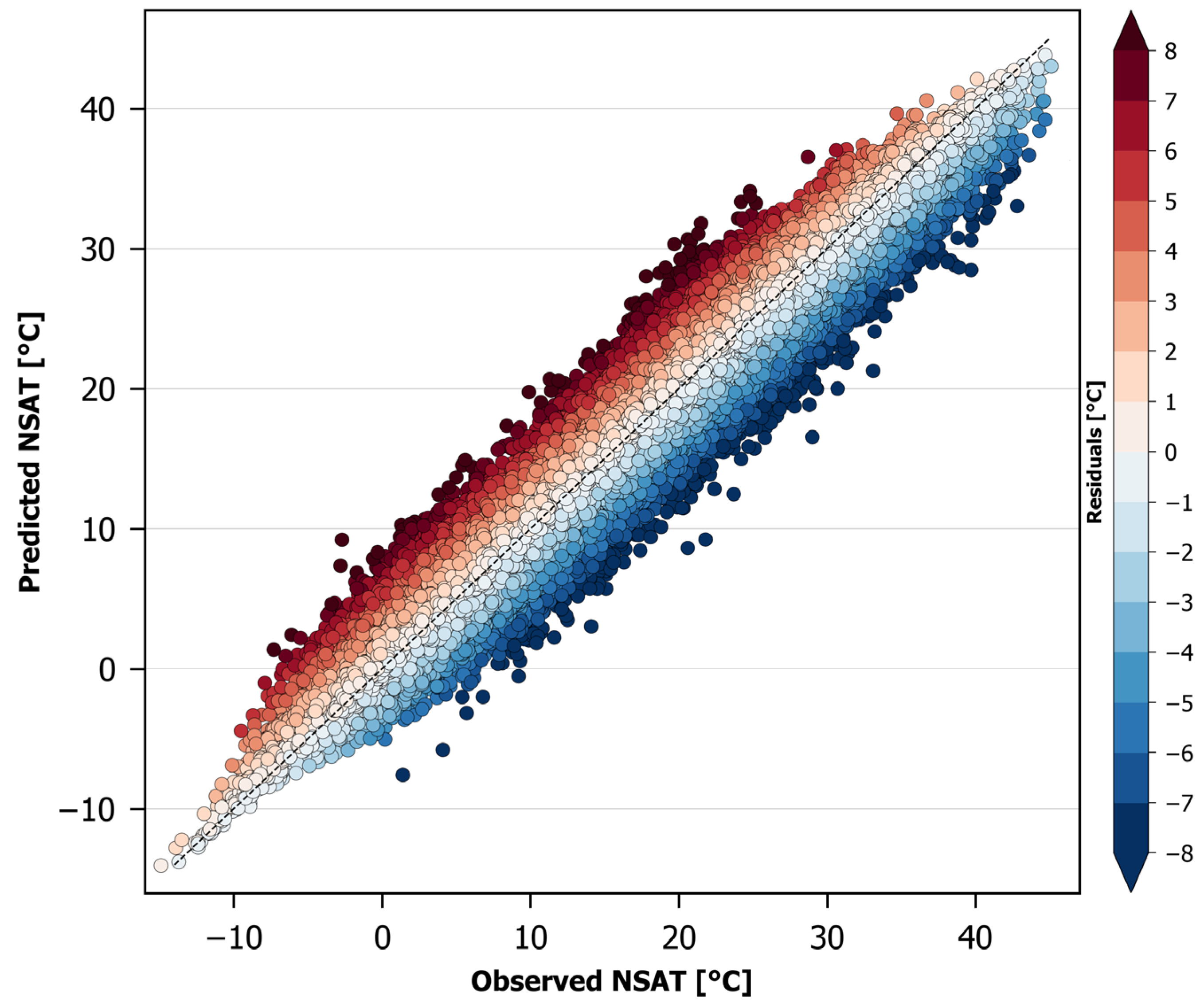
The basic efficiency statistics of the developed model are presented in Table 4. The MAE is below 1 °C (0.96 °C), indicating a quite successful model, especially when compared to previous related works applicable only to cloud-free satellite data, where the MAE ranged from 0.9 °C to over 3 °C. The MBE is −0.01 °C, suggesting a rather random dispersion of the errors above and below the diagonal (Figure 4), with a negligible tendency for underestimation. The RMSE is rather close to the MAE, indicating a limited influence of outliers and similar magnitudes for the individual errors, while the R2 value, which is close to one, supports our argument that the selected model is quite efficient.
Table 4.
Efficiency metrics of the 20 predictors Random Forest model for the NSAT estimation.

Figure 4.
Scatter plot of the NSAT estimation errors of the Random Forest model.
Figure 4 shows a scatter plot of the NSAT estimation errors of the Random Forest model for the complete validation dataset. The graph depicts quite clearly a balanced distribution of errors over and under the diagonal, supporting the minimal MBE (−0.01 °C).
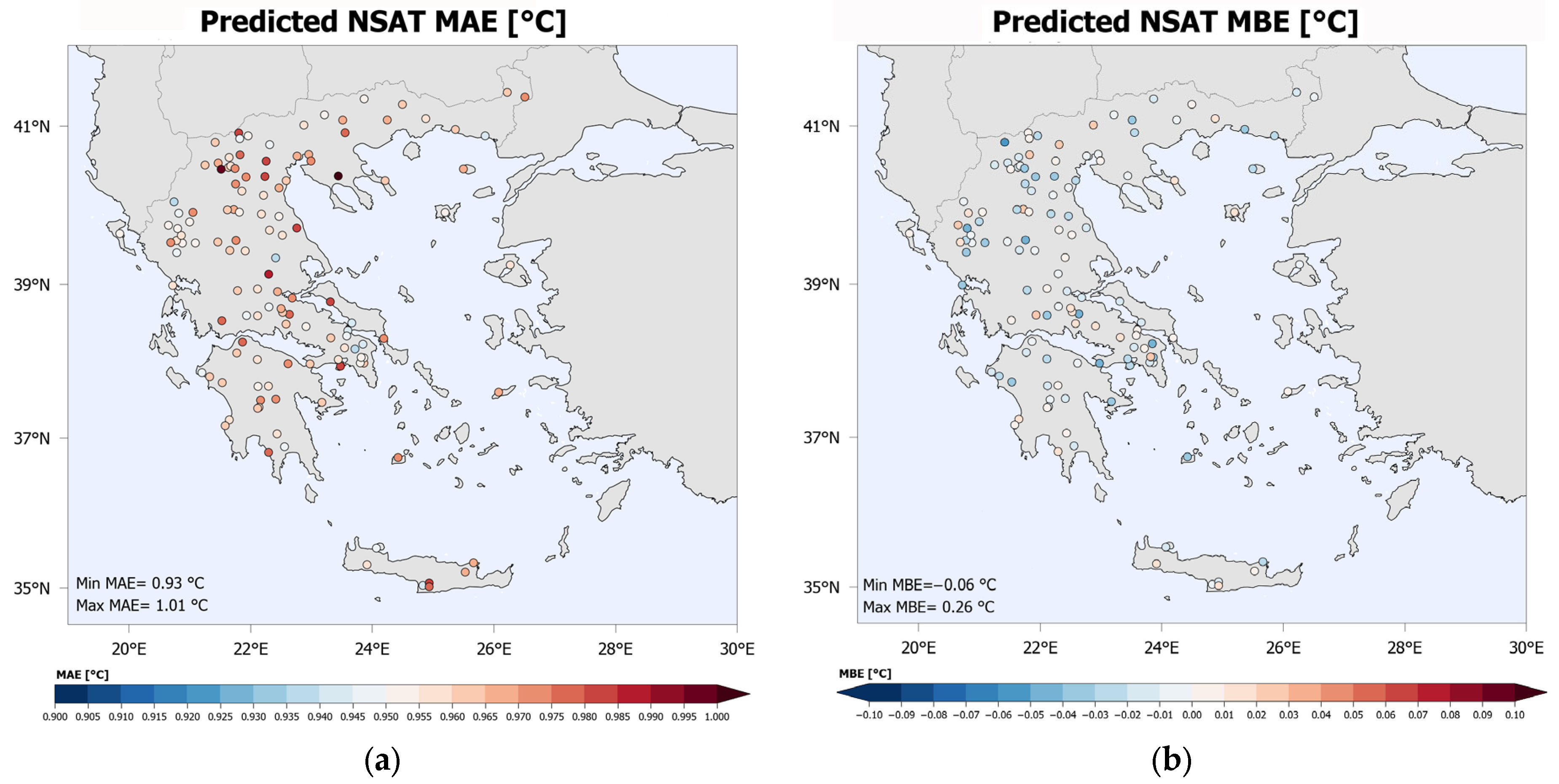
Figure 5 illustrates (a) the MAE and (b) the MBE of the NSAT estimation per station, based, as always on the validation dataset. As shown in the MAE map, the absolute error ranges from 0.93 °C to 1.01 °C, with fluctuations that seem to be rather unrelated to the most basic topographic features (e.g., latitude, longitude, distance to the coast, etc.). The MBE per station ranges from −0.06 °C to 0.26 °C, again with no profound relevance to topography features. Overall, the maps and statistics presented in Figure 5 indicate that the NSAT estimation errors are not significantly influenced by the topography. However, in order to examine in some detail whether a relation between topography and estimation efficiency exists, further analysis is required.
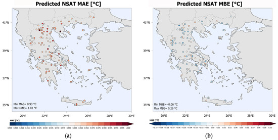
Figure 5.
MAE (a) and MBE (b) of the NSAT estimation per station.
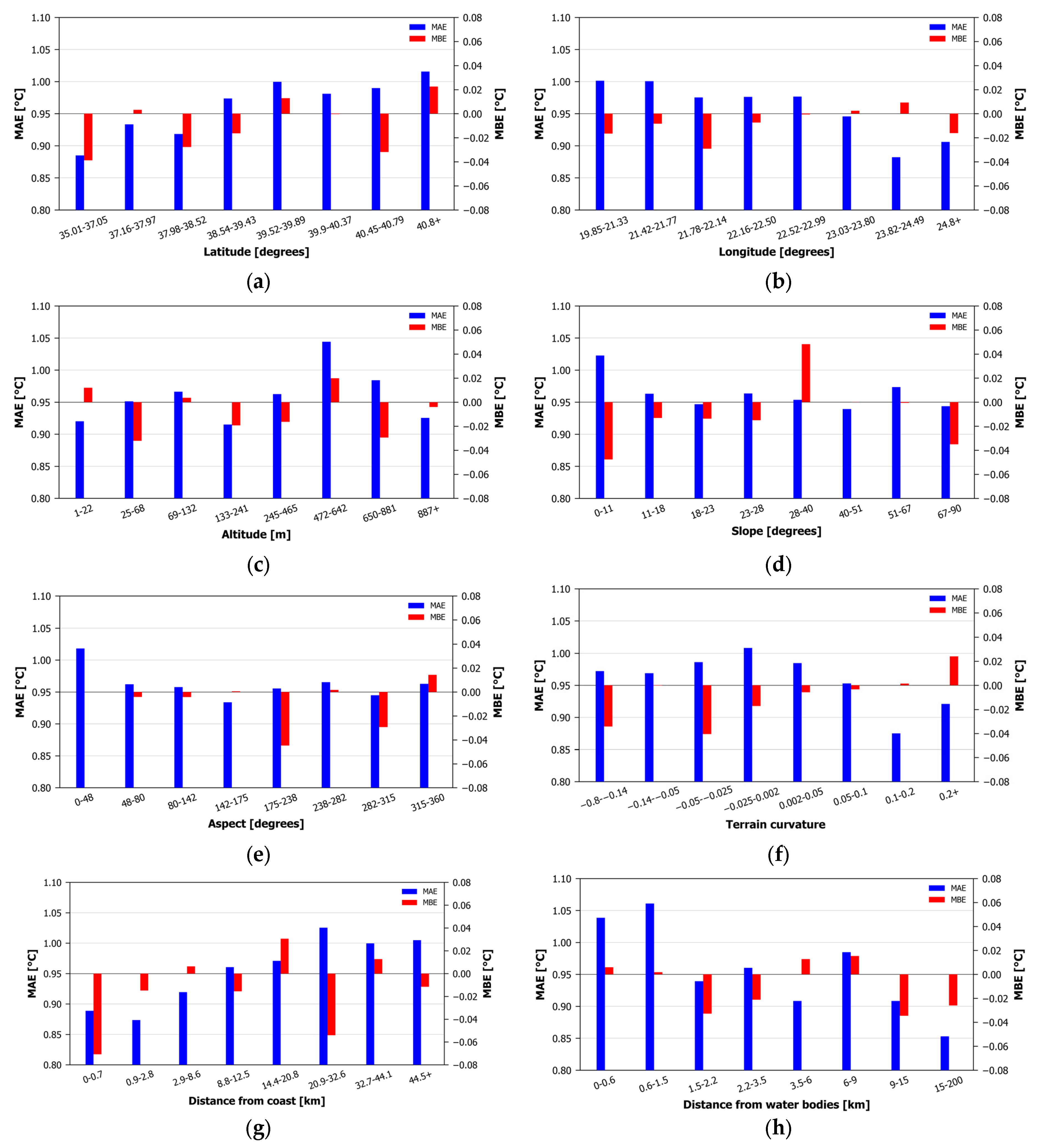
A bin analysis was performed in order to highlight the possible influence of important topographical parameters (namely, elevation, latitude, longitude, distance to the coast, distance to water bodies, slope aspect and terrain curvature) in the estimation efficiency. The validation subset was divided into eight bins and the metrics were calculated for each bin. The bins were formulated in a manner that secured a similar number of stations for each one.
Figure 6 presents bar charts illustrating the MAE and MBE for each of the eight bins of the topographical parameters. Latitude and longitude present small variations in the MAE (ranging from 0.88 °C to 1.02 °C) and MBE (ranging from −0.04 °C to 0.02 °C). A limited increase in the MAE is noted towards northern latitudes and western longitudes. Bias does not seem to present a clear tendency of increase or decrease, neither a preference for a positive nor negative sign, with the increase in these two topographical parameters. The MAE (ranging from 0.92 °C to 1.04 °C) and MBE (ranging from −0.03 °C to 0.02 °C) show small fluctuations with elevation change and no predominance of over- or underestimation. For the slope, the MAE (ranging from 0.94 °C to 1.02 °C) shows a local maximum for slopes up to 11°, followed by small fluctuations. The MBE (ranging from −0.05 °C to 0.05 °C) does not show a preferred tendency. The aspect also shows a local MAE (ranging from 0.93 °C to 1.02 °C) maximum for values below 48° N, followed by small fluctuations afterwards. The MBE (ranging from −0.04 °C to 0.01 °C) minimizes for the 175–238° bin, while, for the rest of the bins, only fluctuations of varying signs exist. The terrain curvature MAE (ranging from 0.88 °C to 1.01 °C) presents a maximum around zero, with fluctuations for the rest of the bins. The MBE (ranging from −0.04 °C to 0.02 °C) shows only fluctuations, with no preference for over- or underestimations. Increasing the distance to the coast seems to slightly increase the MAE (ranging from 0.87 °C to 1.03 °C). The MBE presents small fluctuations (ranging from −0.07 °C to 0.03 °C), with no clear preference for positive or negative bias. Regarding the distance to water bodies, the MAE (ranging from 0.85 °C to 1.06 °C) is slightly higher when close to the water bodies. No systematic bias (with an MBE ranging from −0.03 to 0.01 °C) is noted as we approach water bodies.
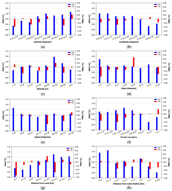
Figure 6.
MAE and MBE for 8 different bins for (a) Latitude, (b) Longitude, (c) Altitude, (d) Slope, (e) Aspect, (f) Terrain curvature, (g) Distance from coast and (h) Distance from water bodies.
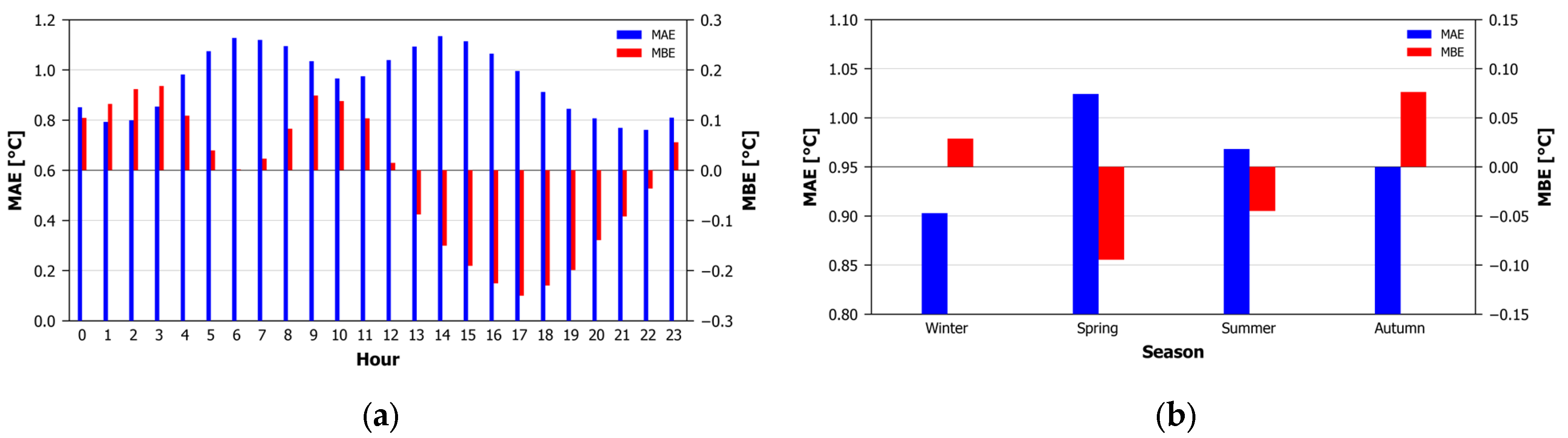
Next, in order to identify the intra-daily and seasonal differences in the estimation efficiency, the validation subset was divided into 24 hourly and 4 seasonal bins, and the metrics were calculated. Figure 7 presents bar charts illustrating the MAE and MBE for each of the 24 h and four seasonal bins. Regarding the intra-daily variation, the MAE (ranging from 0.76 °C to 1.13 °C) presents two local maxima around 06:00 and 14:00 UTC, possibly associated with the more rapid air temperature change during the first morning and first afternoon hours. The MBE (ranging from −0.25 °C to 0.17 °C) presents a general overestimation from the beginning of the 24-h period until 12:00 UTC, and underestimation afterwards (excepting the 23 h bin). On the seasonal level, the MAE ranges from 0.90 °C to 1.02 °C, with winter presenting the lower errors and spring the higher errors. The MBE ranges from −0.09 °C during spring to 0.08 °C during autumn, suggesting mild underestimations during spring and mild overestimations during autumn.
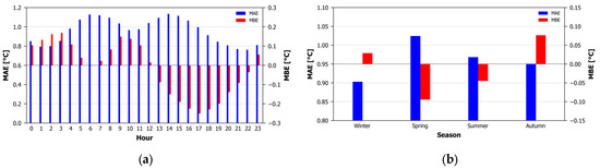
Figure 7.
MAE and MBE for (a) the 4 seasonal and (b) the 24 hourly bins.
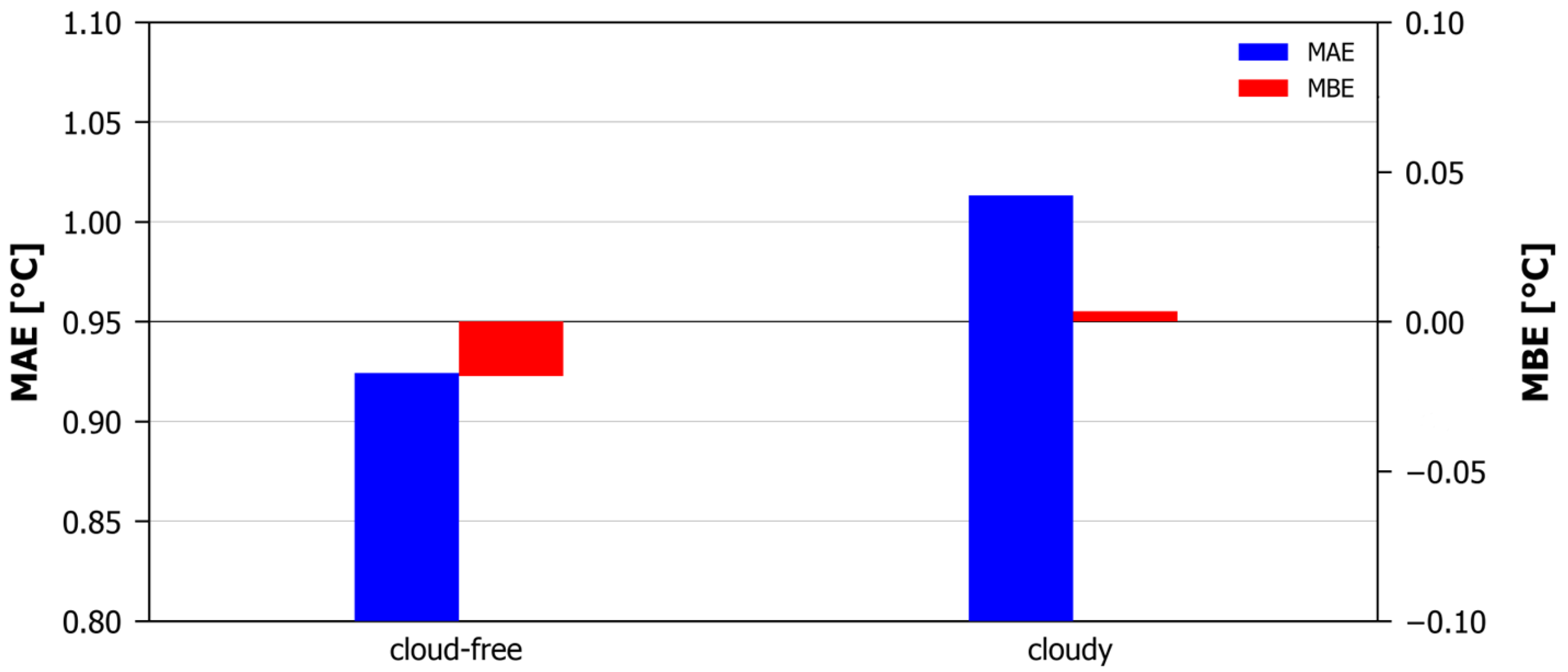
Finally, the possibility of accuracy degradation during cloudy conditions was examined by splitting the validation dataset into cloudy and non-cloudy parts, and through the recalculation of the metrics. The “cloudy” bin includes all pixels characterized as “Cloud filled” or “Pixel contaminated by clouds” by the MLST-AS cloud mask parameter, while the “cloud-free” bin includes all pixels characterized as “Cloud free” by the MLST-AS cloud mask parameter. As seen in Figure 8, under cloud-free conditions, our model estimates the NSAT with an MAE of 0.92 °C and MBE of −0.02 °C. Cloudy conditions result in an MAE of 1.01 °C and an MBE of 0.00 °C. So, as a general rule, NSAT estimations are slightly more accurate under cloud-free conditions, although a marginally stronger underestimation exists compared to the negligible overestimation of the cloudy conditions. It should be noted, however, that the MBE is, in both cases, quite small, suggesting overall that the bias of the model is negligible.

Figure 8.
MAE and MBE for cloud-free and cloudy pixels.
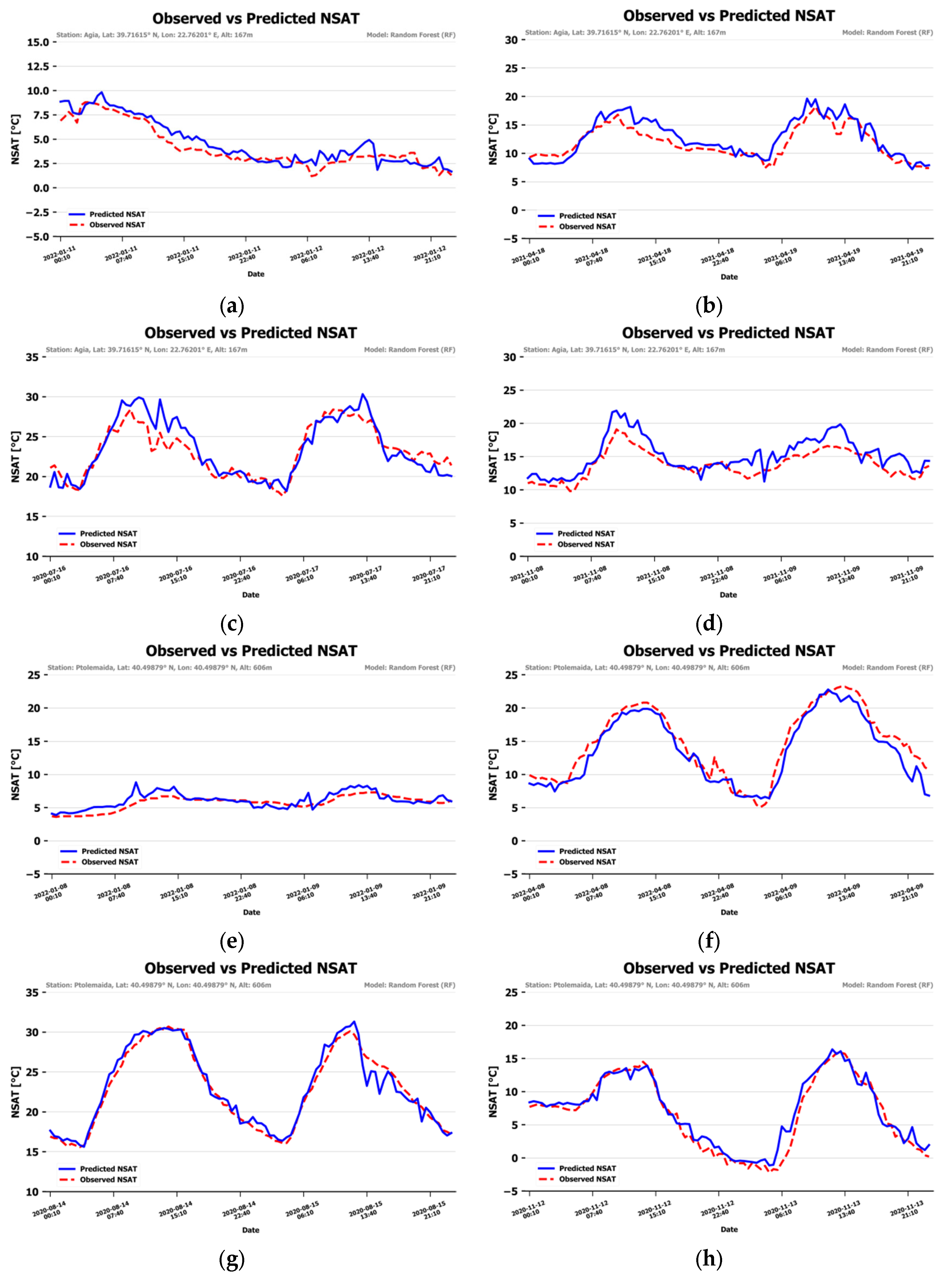
To obtain a visual impression of the accuracy of the NSAT, consecutive days of data in winter, spring, summer and autumn were kept out of the training–validation procedure from two randomly selected stations (Agia and Ptolemaida). The model ran for these data and timelines of NSAT estimations, and the observed values were visualized. Figure 9 presents the graphs. The blue line represents the NSAT estimation and the red dashed line represents the station-observed NSAT. The predicted NSAT follows the observed one quite closely, with slight deviations. Some stronger deviations are noted during the midday and afternoon hours of the first day of the spring subset, the first day of the summer subset and both days of the autumn subset of the Agia station.
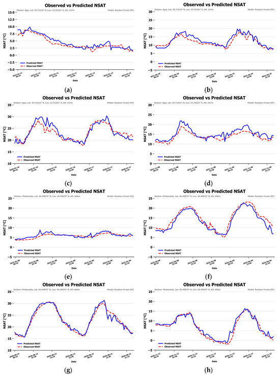
Figure 9.
NSAT predictions vs. temperature observations in winter, spring, summer and autumn for the “Agia” (a–d) and “Ptolemaida” (e–h) weather stations.
4. Potential for Operational Application
Our method for the near-real-time estimation of the NSAT under cloudy and cloud-free conditions using meteorological geostationary satellite data has significant potential for operational use. Areas covered by the LSA SAF required products can provide near-real-time estimations of the NSAT that are completely independent from ground weather stations.
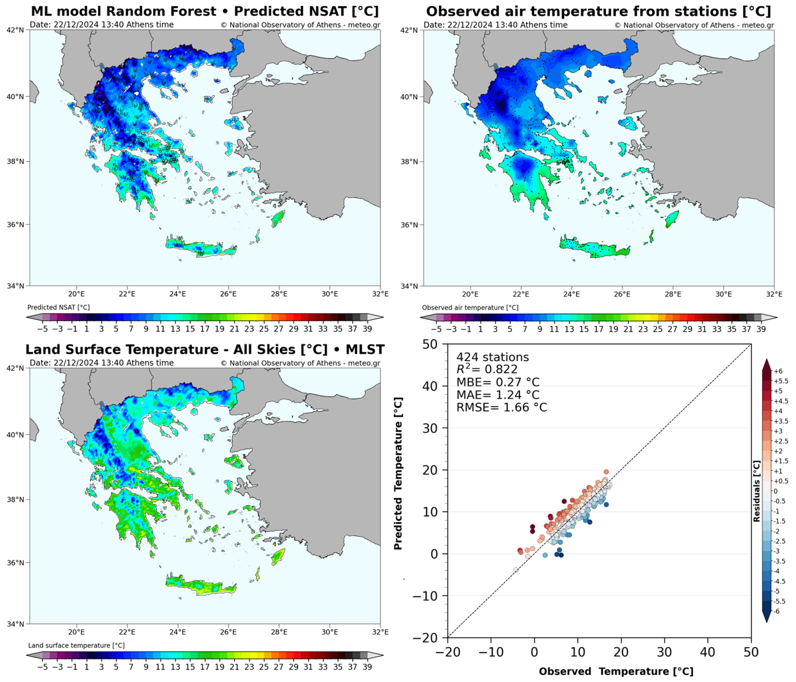
At the METEO Unit at NOA, we implemented such a near-time NSAT estimation procedure used at an experimental level-. At the same time, every-day monitoring of the models’ behavior and estimation efficiency was performed, aiming for the improvement of the product through the identification of strong points and deficiencies. The output of our procedure comprised, among others, a four-image panel (example for 22 December 2024, 13:40 Athens Time, which is shown in Figure 10) depicting the following: a map of the estimated NSAT along with selected weather station observations (top left), a spatially interpolated map of the weather station temperature observations (top right), a map of the most influential LSA SAF parameter of our model, the LST-AS (bottom left) and a scatter plot of the estimation errors, along with some major estimation efficiency statistics (bottom right). The spatially interpolated temperature observation field (top right) does not follow the surface topography, since information about the local differentiations is not included in the interpolation procedure. On the contrary, that information is included in the NSAT estimation procedure, resulting in a more realistic depiction of the temperature. At the same time, a rather good accuracy is achieved. For the specific instance R2, MAE and MBE are equal to 0.822, 1.24 °C and 0.27 °C respectively.
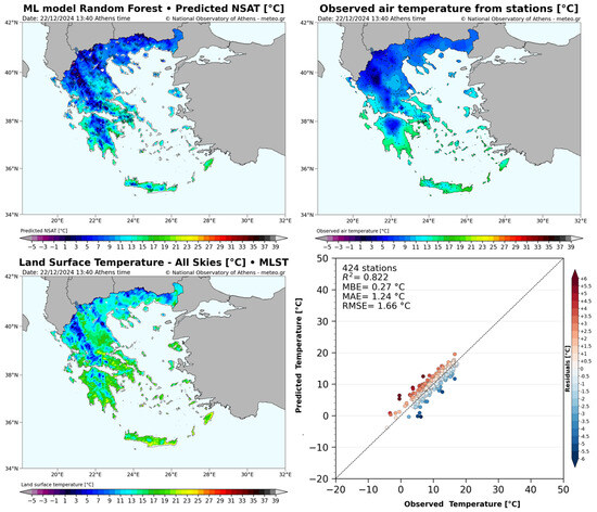
Figure 10.
Operational NSAT estimation panel of the NOA forecasting team: (top left) map of the estimated NSAT along with selected weather station observations; (top right) map of spatially interpolated temperature observations; (bottom left) map of the most important parameter of our model, the LST-AS; (bottom right) scatter plot of the estimation errors, along with major estimation efficiency statistics.
The stability of the half-hourly production of that panel, using standard data acquisition methods for EUMETSAT registered users, ensures that our method could be used operationally for the estimation of the NSAT in all areas covered by the necessary LSA SAF products. National Meteorological Services, research institutes and all kinds of weather-related agencies and organizations can apply and capitalize on similar real-time NSAT estimation procedures. As stated in the Introduction, one major application and benefit of our method is that it could be applied over areas with sparse or absent weather station coverage so to substitute the temperature readings covered by the LSA SAF products.
5. Conclusions
In our present work, the Random Forest machine learning model was employed to estimate the NSAT in near-real-time mode using LSA SAF products, the sun zenith angle and static parameters. Regarding the predictors that seem to be the most influential, we comment the following:
- LST-AS is the predominant parameter. The well-known immediate thermal interaction of land surface and near-surface air masses supports that finding.
- H is the second most influential parameter, which is in agreement with the notion that sensitive heat flux directly affects the air temperature.
- SLF and its 30 min difference are also among the most important features. Incoming longwave radiation directly affects the air temperature and has a significant role in the formulation of the NSAT.
- Cma participates in the formulation of the NSAT, as expected, since the presence of clouds affects the energy budget.
- The rest of the predictors contribute to a much lesser extent. Briefly summarizing the physical mechanisms that connect these parameters to NSAT it is stated that the altitude, slope and terrain curvature relate to the exposure of a site to irradiation, outgoing longwave radiation and also local and synoptic circulation patterns, which directly affect the NSAT. Latitude and longitude are related to the large-scale energy budget and the air masses, which also influence the NSAT. For example, southern areas, in general, have smaller amounts of cloud cover and receive larger amounts of solar radiation. Distance to water bodies and the coastline affect the NSAT through local circulations, latent heat transfer and land–sea energy interactions. The SZA is related to the daily cycle of the NSAT and the formulation of the energy budget at any time of the day. Surface albedo is also amongst the factors that control the amount of incoming radiation that is absorbed by the surface, and therefore the sensible heat that could be provided to the near-surface air masses through conduction, convection and radiation. ET is primarily related to the amount of energy required for evapotranspiration and the release of latent heat in the near-surface air masses. Finally, LAI and FAPAR, two land cover-related parameters, also affect the NSAT through the alteration of important energy budget parameters, for example, the albedo and the sensible and latent heat exchange in their close environment.
The validation dataset estimations of the NSAT were divided into bins of topography and time parameters. The MAE and MBE were computed for these bins, aiming to identify the characteristics, strong points or shortcomings of our model. It was shown that our model is rather unaffected by most of them, with the exception of latitude and longitude, where a mild increase in errors was noted towards the north and west. A mild increase in errors was also noted as we moved away from the coastline and towards water bodies. A limited seasonality exists, while, during the day, the higher errors occur during the first morning and afternoon hours, when the most rapid temperature changes are usually noted. A tendency for overestimation was found until mid-day, with an underestimation afterwards.
Finally, during cyclonic condition predominance, cloudiness is quite increased, and clear sky methodologies fail to estimate the temperature. Our model is able to deliver NSAT estimations regardless of cloudiness and, moreover, in near-real-time mode, provided that access to the required LSA SAF data is secured. The analysis of the overall performance of the model showed only marginally more accurate estimations under cloud-free conditions, supporting our argument that the model is fit to be used regardless of sky conditions.
6. Discussion and Future Work
One of the meteorological parameters that may influence the formulation of the NSAT is the horizontal wind. Air masses can transport sensible and latent heat, affecting the air temperature at local scales. The exclusion of wind data from our model could be considered as a shortcoming. However, if wind data were to be included in the model, dense and high-quality real-time observations would be required. Such data are not always available and, even if found, they might not be representative of the sensible and latent heat transfers, because low-level wind is strongly affected by small-scale topography and anthropogenic constructions, especially in urban and suburban areas. This problem is acknowledged and discussed in previous studies (e.g., [32]). It should also be reminded that temperature estimation is performed at a horizontal resolution of around 5 km, and small-scale wind data might not be representative of the grid-size circulation. The modeled data of comparable horizontal resolution levels could act as an alternative source of wind data. But modeled wind data are forecasts and not observations or even real-time estimations, unavoidably introducing uncertainties that will act as additional sources of errors. Moreover, modeled data may suffer from other innate deficiencies related to the inaccurate representation of topography and human constructions, again especially in urban and suburban areas. The errors occurring even in high-resolution models are discussed, for example, by Zhang et al. [33], Goger et al. [34] and Hu et al. [35]. Since our goal was to create an easy to apply model for the NSAT estimation in near-real-time mode, based on publicly available datasets, we decided to exclude the hard-to-find and uncertainty-ridden wind data. We should also keep in mind that certain algorithms of the LSA SAF products include ECMWF model 10 m wind data [12], partially circumventing the problem.
The model was trained using Python scripting. After training, the model was exported in its final form and saved. The pre-trained model can generate predictions straightforwardly when provided with the necessary statics and dynamic parameters (such as LSA SAF products), on which it was originally trained. The computational time ranges from seconds to minutes, depending on the infrastructure. Generating air temperature estimates for a relatively small region, such as Greece, is efficient and fast. Applying the model to larger regions would require more time, but, based on our estimation, should still be completed within several minutes. Overall, our model has a significant potential for operational use, as it is fast, straightforward and stable, provided that the necessary data are available.
Our model could be run in other mid-latitude regions with similar topographic and climatic characteristics as Greece. The NSAT over Greece varies rather largely from values below zero in winter (−5 °C to −10 °C are frequent, especially in mountainous areas) to over 40 °C in summer (mainly in landlocked, low-elevation areas). More about the Greek climate can be found in [36]. This results in a wide range of temperatures for training and validation, and provides confidence that it could be applied with a similar efficiency to other mid-latitude regions with similar temperature ranges. Nonetheless, a new training/validation over the desired region could be beneficial before application.
A challenging and highly desired next step would be to train and operate the model over areas around the world that are poorly covered by weather stations inside the Meteosat field of view. The operation of the model over Africa, for example, which lacks adequate coverage by weather stations (at least large parts of it), could prove to be quite beneficial for public authorities, environmental and health organizations, stakeholders and the general public of the continent. Moreover, the Meteosat Third Generation Imager 1 (MTG-I1) operational Flexible Combined Imager (FCI) [37,38] data are now available. These data offer higher horizontal and temporal resolution, and more spectral channels. Near-real-time LSA SAF products are also expected to be in the FCI higher resolution. It is anticipated that all of the parameters (derived from MSG SEVIRI) that were used here as predictors for our model will present higher accuracy when derived from FCI data. As a consequence, the retraining of the model over larger areas using FCI data could lead to even higher degrees of accuracy. In our future work, we plan to include such retraining, using Central and Southern Europe and Africa weather station observations as the ground truth, towards the development of an even more accurate and widely applicable model for the estimation of the NSAT.
Author Contributions
Conceptualization, A.K.; methodology, A.K. and G.K.; software, A.K. and G.K.; validation, A.K. and G.K.; formal analysis, A.K., G.K., K.L. and V.K.; investigation, A.K., G.K., K.L. and V.K.; resources, K.L. and V.K.; data curation, A.K. and G.K.; writing—original draft preparation, A.K. and G.K.; writing—review and editing, A.K., G.K., K.L. and V.K.; visualization, A.K. and G.K.; supervision, A.K., K.L. and V.K. All authors have read and agreed to the published version of the manuscript.
Funding
This research was partially funded by the General Secretariat of Research and Innovation (GSRI) under project “CLIMPACT: Support for upgrading the operation of the national network for climate change”, financed by the national section of the PDE National Development Program 2021–2025, Ministry of Development—General Secretariat of Research and Innovation.
Data Availability Statement
The LSA SAF data analyzed are publicly available through the LSA SAF website. No other publicly available datasets were used.
Acknowledgments
The authors wish to acknowledge the contribution of the LSA SAF to this study for the provision of the publicly available datasets and the sun zenith angle data. We also acknowledge partial funding of this research by the project “Climpact: Support for upgrading the operation of the national network for climate change”, financed by the national section of the PDE National Development Program 2021–2025, Ministry of Development—General Secretariat of Research and Innovation.
Conflicts of Interest
The authors declare no conflicts of interest.
References
- Stisen, S.; Sandholt, I.; Nørgaard, A.; Fensholt, R.; Eklundh, L. Estimation of diurnal air temperature using MSG SEVIRI data in West Africa. Remote Sens. Environ. 2007, 110, 262–274. [Google Scholar] [CrossRef]
- Prihodko, L.; Goward, S.N. Estimation of air temperature from remotely sensed surface observations. Remote Sens. Environ. 1997, 60, 335–346. [Google Scholar] [CrossRef]
- Zakšek, K.; Schroedter-Homscheidt, M. Parameterization of air temperature in high temporal and spatial resolution from a combination of the SEVIRI and MODIS instruments. ISPRS J. Photogramm. Remote Sens. 2009, 64, 414–421. [Google Scholar]
- Nieto, H.; Sandholt, I.; Aguado, I.; Chuvieco, E.; Stisen, S. Air temperature estimation with MSG-SEVIRI data: Calibration and validation of the TVX algorithm for the Iberian Peninsula. Remote Sens. Environ. 2011, 115, 107–116. [Google Scholar]
- Shen, S.; Leptoukh, G.G. Estimation of surface air temperature over central and eastern Eurasia from MODIS land surface temperature. Environ. Res. Lett. 2011, 6, 045206. [Google Scholar] [CrossRef]
- Hengl, T.; Heuvelink, G.B.M.; Perčec Tadić, M.; Pebesma, E.J. Spatio-temporal prediction of daily temperatures using time-series of MODIS LST images. Theor. Appl. Climatol. 2012, 107, 265–277. [Google Scholar] [CrossRef]
- Parmentier, B.; McGill, B.; Wilson, A.M.; Regetz, J.; Jetz, W.; Guralnick, R.P.; Tuanmu, M.-N.; Robinson, N.; Schildhauer, M. An Assessment of Methods and Remote-Sensing Derived Covariates for Regional Predictions of 1 km Daily Maximum Air Temperature. Remote Sens. 2014, 6, 8639–8670. [Google Scholar] [CrossRef]
- Janatian, N.; Sadeghi, M.; Sanaeinejad, S.H.; Bakhshian, E.; Farid, A.; Hasheminia, S.M.; Ghazanfari, S. A statistical framework for estimating air temperature using MODIS land surface temperature data. Int. J. Climatol. 2016, 3, 1181–1194. [Google Scholar] [CrossRef]
- Hooker, J.; Duveiller, G.; Cescatti, A. A global dataset of air temperature derived from satellite remote sensing and weather stations. Sci. Data 2018, 5, 180246. [Google Scholar] [CrossRef]
- Hough, I.; Just, A.C.; Zhou, B.; Dorman, M.; Lepeule, J.; Kloog, I. A multi-resolution air temperature model for France from MODIS and Landsat thermal data. Environ. Res. 2020, 183, 109244. [Google Scholar] [CrossRef]
- Nascetti, A.; Monterisi, C.; Iurrilli, F.; Sonnessa, A. A neural network regression model for estimating maximum daily air temperature using Landsat-8 data. ISPRS Arch. 2022, 43, 1273–1278. [Google Scholar] [CrossRef]
- LSA SAF Products Documentation. Available online: https://nextcloud.lsasvcs.ipma.pt/s/zXJoeTf6HByE6RP (accessed on 26 January 2025).
- Huband, N.D.S.; Monteith, J.L. Radiative surface temperature and energy balance of a wheat canopy. Bound.-Layer Meteorol. 1986, 36, 1–17. [Google Scholar] [CrossRef]
- Su, Z. The Surface Energy Balance System (SEBS) for estimation of turbulent heat fluxes. Hydrol. Earth Syst. Sci. 2002, 6, 85–99. [Google Scholar] [CrossRef]
- Ahrens, C.D. Meteorology Today: An Introduction to Weather, Climate, and the Environment, 10th ed.; Thomson/Brooks/Cole: Pacific Grove, CA, USA, 2012; 640p. [Google Scholar]
- Mutiibwa, D.; Strachan, S.; Albright, T. Land surface temperature and surface air temperature in complex terrain. IEEE J. Sel. Top. Appl. Earth Obs. Remote Sens. 2015, 8, 4762–4774. [Google Scholar] [CrossRef]
- EUMETSAT. Available online: https://www.eumetsat.int (accessed on 1 January 2025).
- Land Surface Analysis SAF. Available online: https://landsaf.ipma.pt/en/ (accessed on 1 January 2025).
- Geodata.gov.gr Datasets. Available online: https://geodata.gov.gr/en/dataset (accessed on 1 January 2025).
- Copernicus. Available online: https://land.copernicus.eu/imagery-in-situ/eu-dem/eu-dem-v1.1 (accessed on 1 January 2025).
- Lagouvardos, K.; Kotroni, V.; Bezes, A.; Koletsis, I.; Kopania, T.; Lykoudis, S.; Mazarakis, N.; Papagiannaki, K.; Vougioukas, S. The automatic weather stations NOANN network of the National Observatory of Athens: Operation and database. Geosci. Data J. 2017, 4, 4–16. [Google Scholar] [CrossRef]
- Meenal, R.; Michael, P.A.; Pamela, D.; Rajasekaran, E. Weather prediction using random forest machine learning model. Indones. J. Electr. Eng. Comput. Sci. 2021, 22, 1208–1215. [Google Scholar] [CrossRef]
- Suthar, G.; Singh, S.; Kaul, N.; Khandelwal, S.; Singhal, R.P. Prediction of maximum air temperature for defining heat wave in Rajasthan and Karnataka states of India using Machine Learning Approach. Remote Sens. Appl. 2023, 32, 101048. [Google Scholar] [CrossRef]
- Osman, A.I.A.; Ahmed, A.N.; Chow, M.F.; Huang, Y.F.; El-Shafie, A. Extreme gradient boosting (Xgboost) model to predict the groundwater levels in Selangor Malaysia. Ain Shams Eng. J. 2021, 12, 1545–1556. [Google Scholar] [CrossRef]
- Tran, T.T.K.; Bateni, S.M.; Ki, S.J.; Vosoughifar, H. A review of neural networks for air temperature forecasting. Water 2021, 13, 1294. [Google Scholar] [CrossRef]
- Kyros, G.; Manolas, I.; Diamantaras, K.; Dafis, S.; Lagouvardos, K. A machine learning approach for rainfall nowcasting using numerical model and observational data. Procedia Environ. Sci. 2023, 26, 11. [Google Scholar]
- Chen, T.; Guestrin, C. XGBoost: A scalable tree boosting system. In Proceedings of the 22nd ACM SIGKDD International Conference on Knowledge Discovery and Data Mining, San Francisco, CA, USA, 13–17 August 2016. [Google Scholar]
- Roy, D.S. Forecasting the air temperature at a weather station using deep neural networks. Procedia Comput. Sci. 2020, 178, 38–46. [Google Scholar] [CrossRef]
- Chattopadhyay, S.; Jhajharia, D.; Chattopadhyay, G. Univariate modelling of monthly maximum temperature time series over northeast India: Neural network versus Yule–Walker equation based approach. Meteorol. Appl. 2021, 18, 70–82. [Google Scholar] [CrossRef]
- Anjali, T.; Chandini, K.; Anoop, K.; Lajish, V.L. Temperature Prediction using Machine Learning Approaches. In Proceedings of the 2nd International Conference on Intelligent Computing, Instrumentation and Control Technologies (ICICICT), Kannur, India, 5–6 July 2019. [Google Scholar]
- WWRP/WGNE Joint Working Group on Forecast Verification Research: Forecast Verification Methods Across Time and Space Scales. 2015. Available online: https://www.cawcr.gov.au/projects/verification/ (accessed on 1 January 2025).
- Benali, A.; Carvalho, A.C.; Nunes, J.P.; Carvalhais, N.; Santo, A. Estimating air surface temperature in Portugal using MODIS LST data. Remote Sens. Environ. 2012, 124, 108–121. [Google Scholar] [CrossRef]
- Zhang, H.; Pu, Z.; Zhang, X. Examination of Errors in Near-Surface Temperature and Wind from WRF Numerical Simulations in Regions of Complex Terrain. Weather. Forecast. 2013, 28, 893–914. [Google Scholar] [CrossRef]
- Goger, B.; Rotach, M.W.; Gohm, A.; Stiperski, I.; Fuhrer, O. Current challenges for numerical weather prediction in complex terrain: Topography representation and parameterizations. In Proceedings of the 2016 International Conference on High Performance Computing & Simulation (HPCS), Innsbruck, Austria, 18–22 July 2016. [Google Scholar]
- Hu, S.; Xiang, Y.; Zhang, H.; Xie, S.; Li, J.; Gu, C.; Sun, W.; Liu, J. Hybrid forecasting method for wind power integrating spatial correlation and corrected numerical weather prediction. Appl. Energy 2021, 293, 116951. [Google Scholar] [CrossRef]
- Feidas, H.; Karakostas, T.; Zanis, P. The wonderful weather of Greece. In The Geography of Greece, 1st ed.Darques, R., Sidiropoulos, G., Kalabokidis, K., Eds.; World Regional Geography Book Series; Springer: Cham, Switzerland; pp. 413–429.
- Ouaknine, J.; Viard, T.; Napierala, B.; Foerster, U.; Fray, S.; Hallibert, P.; Durand, Y.; Imperiali, S.; Pelouas, P.; Rodolfo, J.; et al. The FCI on board MTG: Optical design and performances. In Proceedings of the International Conference on Space Optics—ICSO 2014, La Caleta, Spain, 7–10 October 2014. [Google Scholar]
- EUMETSAT—Meteosat Third Generation Instruments. Available online: https://www.eumetsat.int/meteosat-third-generation-instruments (accessed on 3 March 2025).


Disclaimer/Publisher’s Note: The statements, opinions and data contained in all publications are solely those of the individual author(s) and contributor(s) and not of MDPI and/or the editor(s). MDPI and/or the editor(s) disclaim responsibility for any injury to people or property resulting from any ideas, methods, instructions or products referred to in the content. |
© 2025 by the authors. Licensee MDPI, Basel, Switzerland. This article is an open access article distributed under the terms and conditions of the Creative Commons Attribution (CC BY) license (https://creativecommons.org/licenses/by/4.0/).