Adopting an Open-Source Processing Strategy for LiDAR Drone Data Analysis in Under-Canopy Archaeological Sites: A Case Study of Torre Castiglione (Apulia)

Abstract

This study introduces a methodology for the improvement of the visibility of archaeological features using an open-source probabilistic machine learning framework applied to UAV LiDAR data from the Torre Castiglione site in Apulia, Italy. By leveraging a Random Forest classification algorithm embedded in an open-source software, the approach processes dense LiDAR point clouds to segment out vegetation from the ground and the structures. Key steps include training the classifier, generating digital terrain models, digital feature models, and digital surface models, and enhancing the visibility of archaeological features. This method has proven effective in improving the interpretation of archaeological sites, revealing previously hidden or difficult-to-access microtopographic and structural details, such as the defensive structures, terraces, and ancient paths of the Torre Castiglione site. The results underline this methodology’s ease of use in uncovering archaeological landscapes under a dense canopy. Moreover, the study emphasises the benefits of using open-source tools to enhance the documentation and analysis of remote or difficult archaeological sites.

1. Introduction

In the 21st century two technological innovations have significantly reshaped the archaeological field: LiDAR (Light Detection and Ranging) for data collection, and drones, also known as Unmanned Aerial Systems (UAS). These technologies have greatly expanded the scope of archaeological investigations, enabling the access to areas obscured by dense vegetation and providing a cost-effective alternative to traditional aerial methods based on planes or helicopters.

The synergy between UAS and LiDAR technologies has proven to be very effective, increasing the accessibility of aerial LiDAR to research institutions, universities, and independent archaeologists worldwide. The widespread availability of LiDAR data has, in turn, spurred the development of a variety of processing tools and open software codes. These tools primarily focus on the classification and segmentation of the point clouds generated by LiDAR, thus facilitating the identification of archaeological features as well as the production of the following Digital Models (DMs): (i) Digital Elevation Models (DEMs), (ii) Digital Surface Models (DSMs), and (iii) Digital Feature Models (DFMs) [1,2,3,4]. Digital Surface Models (DSM) capture the surface of a scene exactly as it appears from above, including all objects and vegetation present at the time the data were captured. On the other hand, Digital Terrain Models (DTM) are fundamental in fields such as topography, environmental sciences and landscape studies, as they provide a clean view of the terrain, free of any surface objects or vegetation. This makes DTMs particularly useful for creating topographic maps and contour lines. On the other hand, in the field of archaeology, Digital Feature Models (DFMs) are particularly valuable. These models offer a digital view of the area recorded by LiDAR technology, keeping visible structures, those partially or completely covered by vegetation, and the ground, which is essential for revealing details useful for archaeological research [4].

Airborne LiDAR technology is not a technique that was developed purely for archaeological purposes [5,6]. In fact, starting from the second half of the 20th century, the idea of using airborne lasers for topographical and urban planning purposes [7,8,9] and for studying oceans [10,11] and vegetation [12,13,14] was developed. The first archaeological studies related to the use of LiDAR were carried out in the 1960s, although it is only since the 21st century that this technology has been widely used in archaeology [15]. During this period, LiDAR has become increasingly popular in archaeology, thanks also to the reduction in costs and the ease of use, and has opened up new perspectives, becoming a game changer in archaeological research [16,17,18,19,20,21,22,23,24,25,26,27,28,29,30,31,32,33,34]. This revolution occurred mainly due to the possibility of being able to investigate, in a short time, at relatively low cost compared to traditional archaeological surveys, and in a safe way, large areas densely covered by vegetation [35,36]. Many studies have demonstrated the effectiveness of LiDAR in revealing archaeological sites covered by vegetation, with remarkable results, such as (i) Khan et al. [37] in the Amazon, (ii) Chase et al. [16,21] on Maya civilisations, and (iii) Evans et al. [18,38] at Angkor Wat. Furthermore, many LiDAR datasets are now made public by national authorities and free to use. These have average density and resolutions ranging from 1 to 20 points per m² and 1 to 5 m (in DMs resolution), representing an excellent tool to identify features of archaeological interest, according to the literature [39,40,41,42,43,44].

Current advances in LiDAR technology also include data filtering and feature extraction using machine learning and deep learning, thus offering new perspectives in both supervised and unsupervised detection of archaeological features [1,42,45,46,47,48].

Today, one the main challenges in LiDAR data processing is the complexity of classification and segmentation of point clouds. In recent years, several open and commercial software tools have been released to address these challenges. These include various filtering techniques applied to point clouds, such as morphological filters, progressive triangular irregular networks, surface-based and segmentation-based filtering, and hybrid filters [17,49,50,51,52,53,54,55].

This paper proposes a completely open-source approach to the analysis of LiDAR data for archaeological purposes, based on a probabilistic random forest algorithm and developed through a series of methodological stages exploiting a limited set of free tools. The main objective is to make the use of the advanced remote sensing and machine learning techniques that have become more accessible and replicable for archaeological investigations, allowing a growing number of researchers and practitioners to benefit from automated and efficient procedures in the detection of potential traces of historical and cultural interest. The strength of this research lies in the combination of free tools, such as (i) CloudCompare v.2.14 (3DMASC plugin), (ii) RVT v.2.2.1 (stand-alone version) for image enhancement [56,57,58], (iii) and QGIS v. 3.28.2 for cartographic processing and visualisation, into a coherent and efficient workflow. This combination, supported by a rigorous evaluation of the machine learning model’s performance metrics, contributes to the creation of an integrated data analysis and mapping system: a system capable of improving and enhancing archaeological information during the interpretation and planning of excavations and reconnaissance, as well as the maintenance and preservation of cultural heritage.

2. Materials and Methods

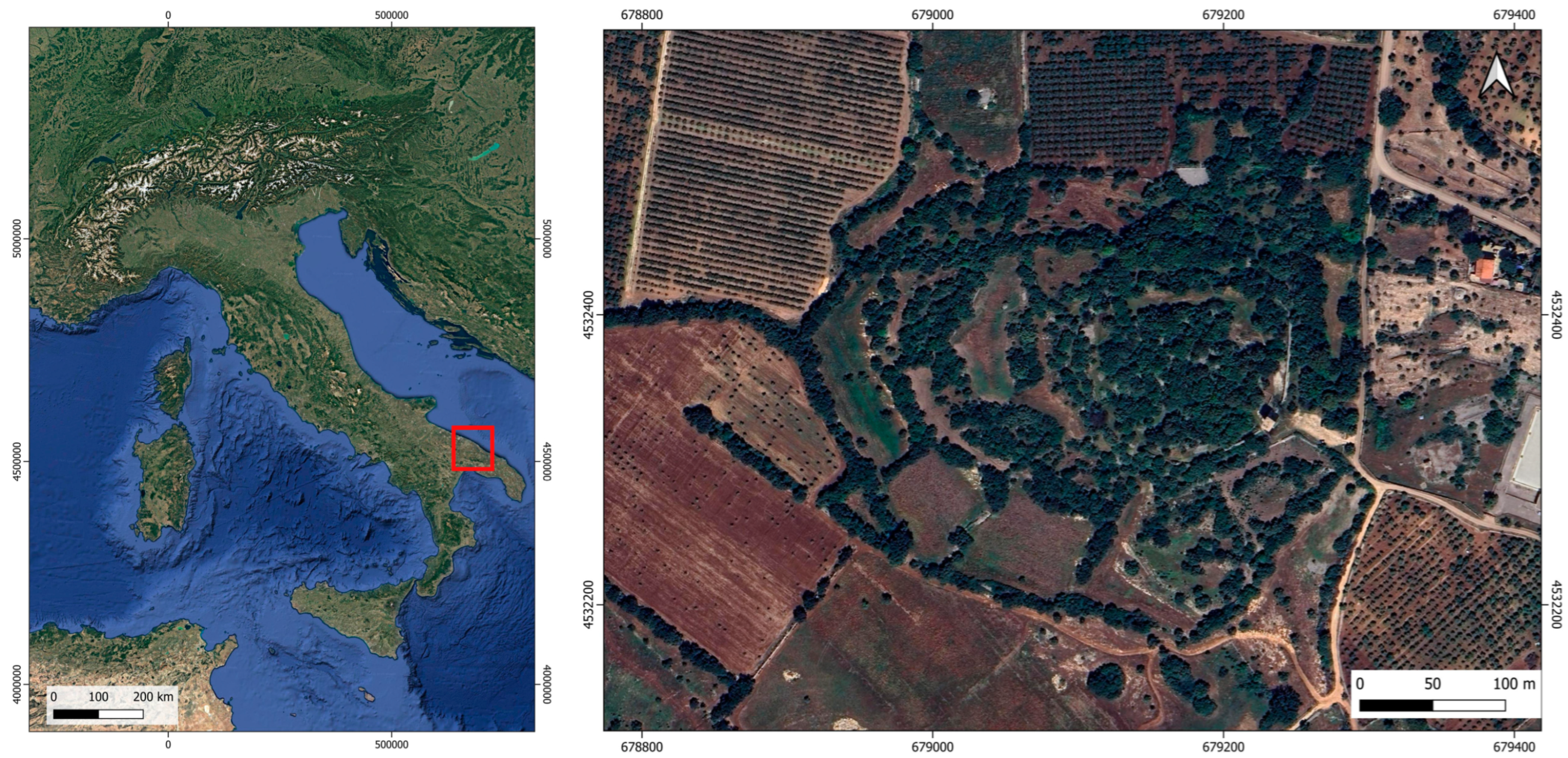
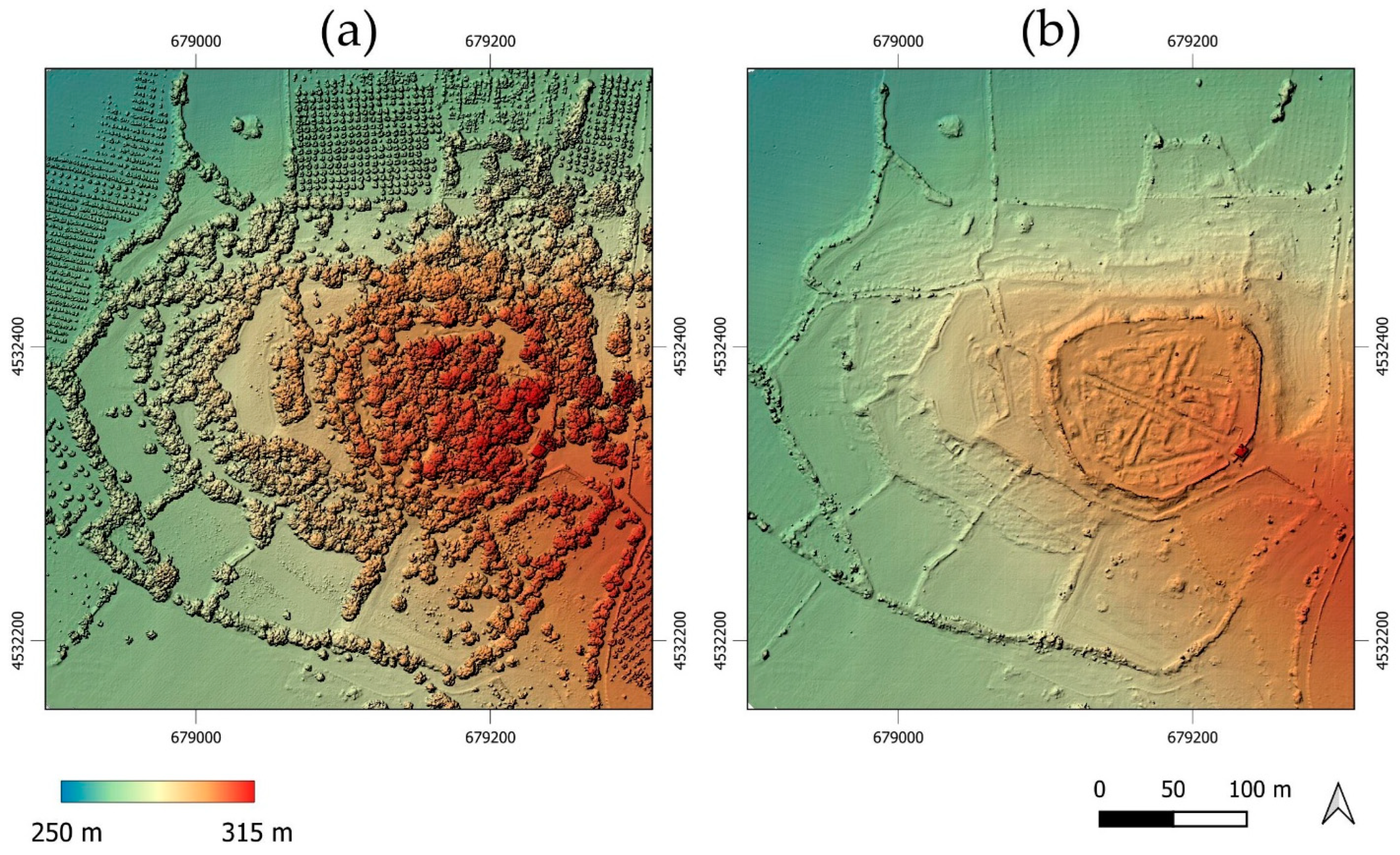
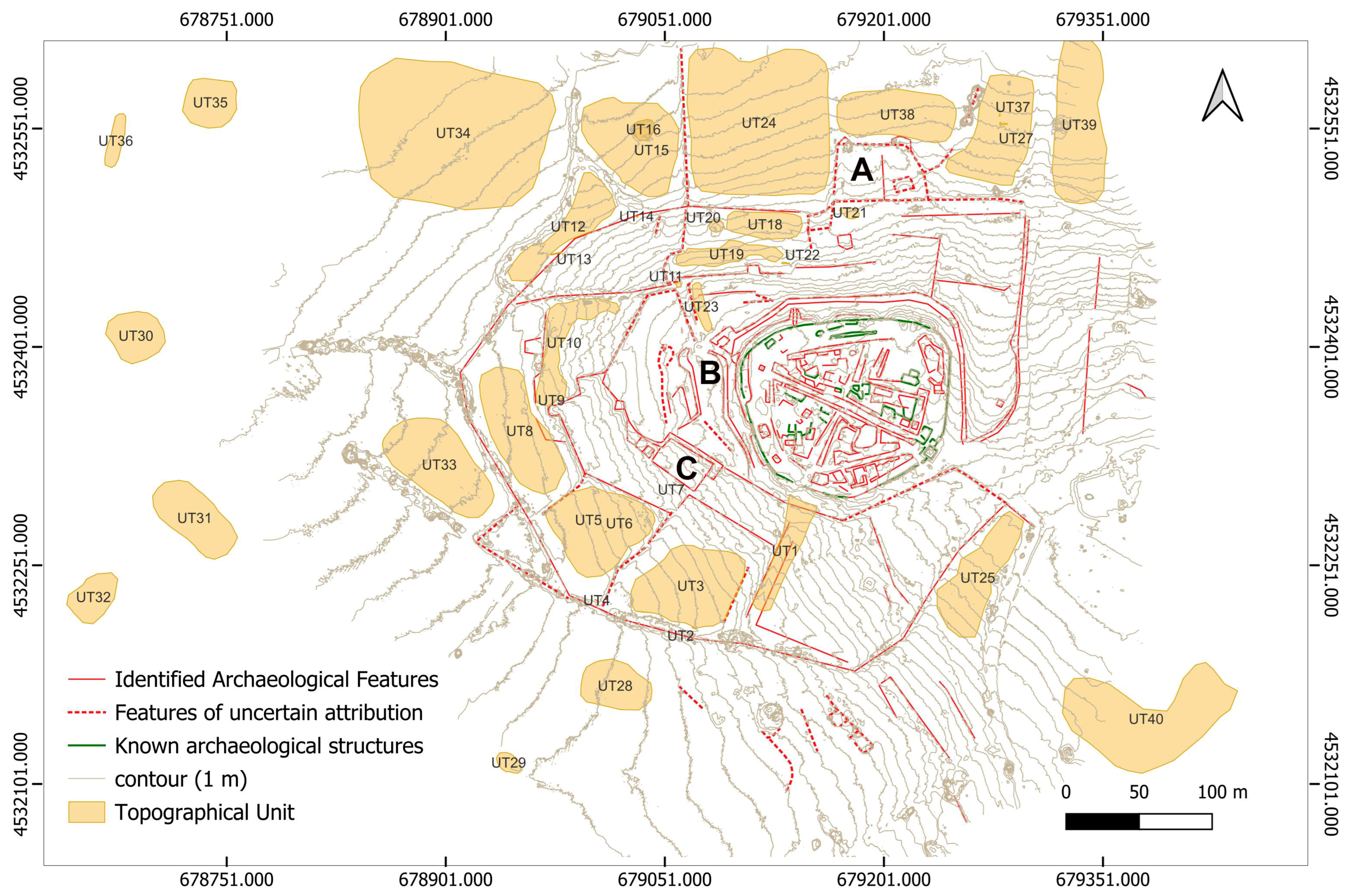
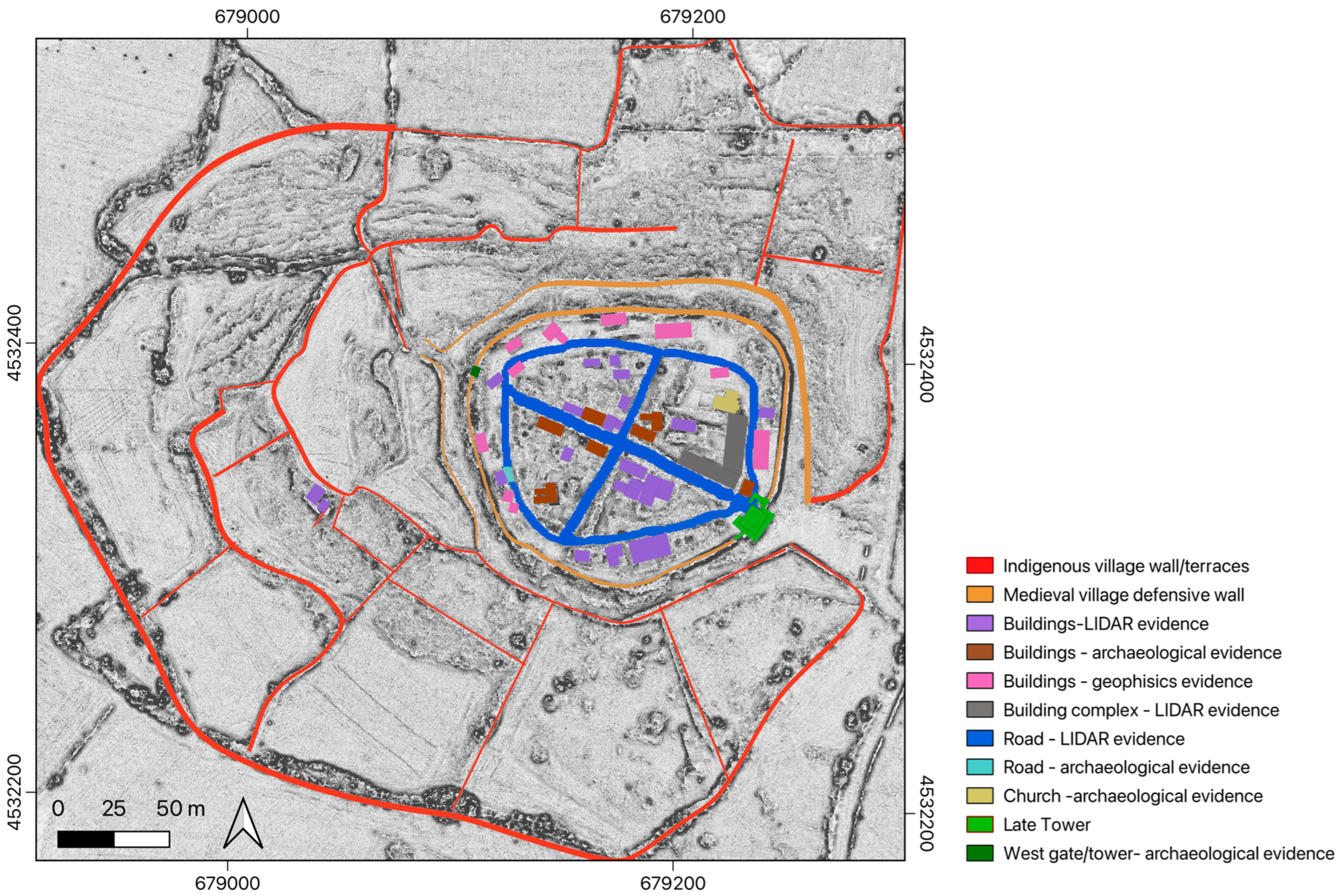
2.1. Study Area

The case study is the hill of Castiglione, located a few kilometres away from Conversano, a small urban centre in the province of Bari. The territory of Conversano is one of the most interesting testimonies to the dense, complex, centuries-old history of the Murgia district in south-eastern Apulia (Figure 1). The Murge is a sub-region stretching between the central Apulia and the Nord-eastern Basilicata and consists of karstic plateau of tectonic origin.

The hill was the site of a fortified settlement of unknown configuration from the 8th–7th century BC, but which probably extended along the slopes and the surrounding flat areas at the height of its expansion [59,60,61,62]. To date, no material evidence or written sources are available to shed light on the events that affected the hillside in the long period between the abandonment of the indigenous village (end of the 4th–3rd century BC) and the Angevin age. In fact, the so far known documentary and archaeological evidence of the rural aggregate settlement of Castiglione, first defined as a terra and then as a casale, dates from the 14th to the mid-15th century [63,64,65,66]. Of this rural casale, the mighty fortification walls, approximately 5 m high and 440 metres long, and a small church, with a simple single-room plan, still survive. Other ruins of the mediaeval citadel can be found beneath the thick blanket of spontaneous vegetation and maquis shrubland that gradually covered the entire area after the abandonment of the settlement, restoring the hill to its natural appearance.

The attraction exerted by the nearby Conversano, the seat of feudal power and a city in full expansion, and the need for protection, exacerbated after the death of Count Giulio Antonio I of Conversano in the Terra d’Otranto fight against the Ottomans (1481), were perhaps the factors that gave impetus to a slow migration from the hamlet to the city at the end of the 15th century.

At the turn of the 16th century, however, the Castiglione hill would not have appeared completely abandoned: in fact, the monumental lookout tower, about 15 m high, may date back to the beginning of the same century, and still stands along the eastern stretch of the walls. The structure was conceived to serve as a place of defence and as a watchtower, as suggested by the entrance located at a height of 5 metres above ground level, accessible via a drawbridge, and the massive perimeter walls.

It is not known how long the tower fulfilled its function as a military garrison, nor is it possible to place in time the activities that continued to take place on the hill, affecting the visible ruins of the casale: from the spoliation of the church of the Annunziata to the widespread stone-stripping that was undertaken to pile up the rubble of the settlement.

Castiglione never ceased to be occupied: until the 1960s–1970s, the casale’s plain, at the time not yet extensively “reconquered” by the shrubland, was cultivated with olive groves. Here, the shepherds led their flocks of sheep and goats to graze near the high ground, perpetuating the “ancient” custom. Archaeologists have investigated Torre di Castiglione since the late 19th century, when the first official report describing the remains still visible was made public by the Royal Inspector of Excavations [61]. During the 20th century, limited excavations were conducted in 1957–1958, 1981–1983 and 1997–1999, both inside and outside the walls [62,67]. Such archaeological investigations included excavations, reconnaissance, and geophysical analyses.

The identification of the medieval settlement on the top of the hill includes the walls, the area of the watchtower, the church, and two or three 14th-century buildings uncovered during past investigations.

In an area of approximately 500 m² around the site field, the reconnaissance identified 44 topographic units or UT (i.e., any type of evidence, whether movable or immovable, in any state of preservation, that can be identified during a survey covering an area of approximately 150 hectares and that attests to human presence or activity in a specific area), including 13 wall structures, and numerous areas of pottery fragments. The materials found on the surface belong to different ceramic classes: impasto-pottery, matt-painted, achroma, geometric, black-glazed, sealed, bend decorated pottery, glazed, and enamelled pottery, and post-medieval materials. The structures refer to several tombs (UT 6, 14), one tumulus (Figure 2, UT 20), several retaining and terracing walls (Figure 2, UT 4, 9, 13, 22), probable buildings (Figure 2, UT 2, 26, 37), a rock-cut well (Figure 2, UT 7) and a shepherd’s shelter (Figure 2, UT 11). Further reconnaissance, performed in the central area of the site, allowed the identification of 19 walled structures [68] (Figure 2).

2.2. Rationale and Approach

The Torre Castiglione site is now almost entirely covered by dense vegetation, consisting mainly of Mediterranean scrub, olive trees, and tall trees. Currently, only the following features are clearly visible: (i) the structures related to the walls; (ii) the tower in the eastern sector; and (iii) a few structures investigated by archaeological excavation in the north-eastern sector of the walls (Figure 1).

Given its nature as a fortified site with existing structures and its dense vegetation, preventing its full understanding, Torre Castiglione represented the perfect case study for applying a drone-based LiDAR technology. Additionally, a probabilistic supervised machine learning approach was employed to segment point cloud elements effectively. Such a method was adopted to solve the difficulties in properly segmenting and separating the points into classes using automatic algorithms caused by (i) the interaction between vegetation and structures and (ii) the irregularity of the structures below or adjacent to the vegetation. The present study applied the workflow described in the flowchart in Figure 3. It can be divided into two main processes:

(i) The first part focuses on the segmentation of the LiDAR point cloud using probabilistic machine learning algorithms and generation and enhancement of the DSM, DTM, and DFM.

(ii) The second part, focused purely on archaeological research, and centres on the bibliographic research on the site, including the documentation of previous surveys and archaeological excavations, the use of DFMs and derived DFMs in a GIS environment to understand the spatial development of the archaeological site of Torre Castiglione

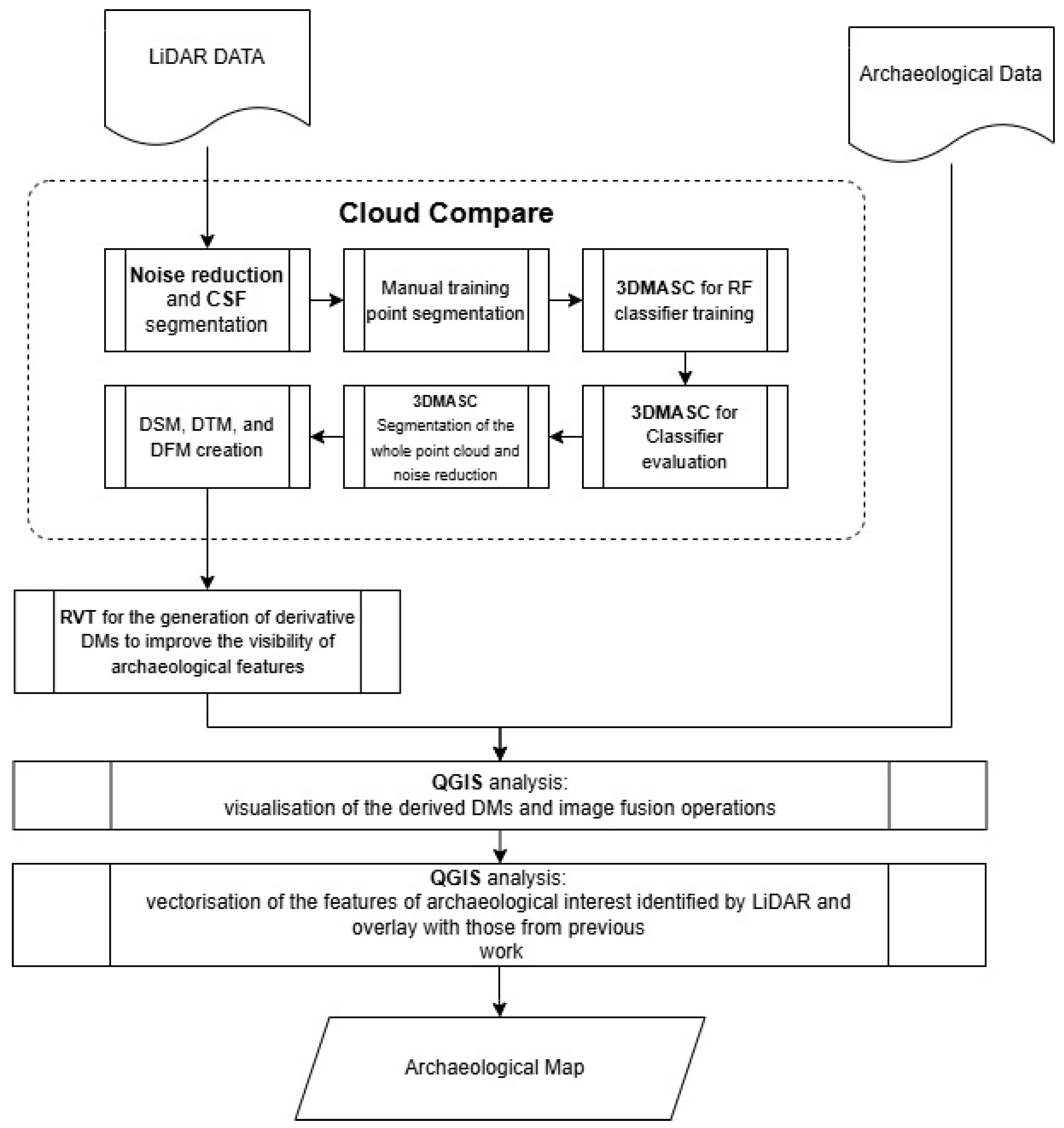
2.2.1. Processing and Segmentation of LiDAR Data from UAVs Using a Probabilistic Supervised Machine Learning Algorithm

Active sensors operate as both the emitters and receptors of signals, thus facilitating a highly precise data acquisition. These sensors can achieve an accuracy in the order of millimetres (in the case of high-precision laser scanners) or centimetres (in the case of environmental laser scanners or UAS LiDAR), enabling the precise spatial localization of reflected data points on and beneath the surface. In particular, laser sensors are appropriate to rapidly collect extensive datasets of objects with complex geometries, thus ensuring a high degree of measurement reliability. Despite their robust performance, the substantial cost and sometimes bulky dimensions of these tools can limit their deployment in resource-constrained or spatially restricted environments. In the domain of archaeological research, technologies such as LiDAR have long since proven to be very useful. They enable a detailed examination of architectural artefacts, penetration of vegetative cover to analyse hidden contexts, and the identification of microtopographic variations indicative of buried archaeological remains [16,20,30,51,69,70,71,72].

The LiDAR survey at Torre Castiglione was performed using a Riegl MiniVux-3, 5-echo LiDAR, equipped with a GNSS PPK positioning system, used as a payload on a DJI Matrice 600 drone. The LiDAR acquisition covered a total area of approximately 25 hectares. The flight was conducted at an altitude of 70 m A.G.L. (Above Ground Level) at a constant speed of 3 m/s, in dual-acquisition grid mode, with UGCS pro software, in Terrain Follow mode. This type of acquisition has proven to be useful in the field of archaeological research with LiDAR data [30]. The steps for processing the LiDAR-acquired data into the georeferenced raw point cloud were (i) the acquisition of GNSS data from the Italian national fixed stations; (ii) the correction of the route acquired by the PPK antenna based on the data from the fixed stations, in Applanix POSPac UAV software (v.9.2); and (iii) the use of Riegl’s RiPROCESS^®® suite (v.1.9) for creating and exporting the point cloud to the WGS 84 UTM 33 N (EPSG: 32633) system. The average point cloud density produced was about 853.23 pnt/m² (Figure 4).

Once the point cloud was generated, a workflow completely based on open-source tools was used to segment the point cloud and improve the obtained results. The workflow was developed using CloudCompare software (v.2.14) to achieve the following:

(1)

Remove outliers and resample the point cloud with minimum point spacing of 0.1 m;

(2)

Segment the ‘ground’ from the ‘off-ground’ using a CSF filter (Cloth Simulation Filter);

(3)

Manually segment a small portion of the ‘off-ground’ point cloud;

(4)

Train a classification algorithm based on probabilistic machine learning (Random Forest) using the 3DMASC plug-in;

(5)

Evaluate the classification algorithm;

(6)

Apply classification to the entire off-ground point cloud;

(7)

Application of CloudCompare’s ‘split’ function to divide ‘vegetation’ points from ‘non-vegetation’ points;

(8)

Clean up the ‘non-vegetation’ cloud through the use of a SOR (Statistical Outlier Removal) and noise filter to remove misclassified points;

(9)

Merge the ‘ground’ point cloud with the classified point cloud (without vegetation and noise) and obtain the data from which to extract the DFM;

(10)

Generate DTM, DSM, and DFM at 0.2 m/pixel resolution.

In detail, 3DMASC (points 3–6) enables the supervised classification of 3D points, exploiting multiple attributes at various scales, using data from single or multiple point clouds.

The classification mechanism employs a Random Forest (RF) algorithm [74,75] to rapidly generalise and apply models to extended datasets, incorporating a function to exclude misclassified points based on their prediction confidence. Random Forest is a supervised classification algorithm in machine learning that uses multiple decision trees built independently on random subsets of data (clustering) and random selections of features. Each tree independently contributes to the final decision, which usually emerges through majority voting, improving the stability of the model and reducing variance. By introducing randomness in both the selection of samples and the selection of features, Random Forest minimises the correlation between trees and significantly reduces overfitting, leading to robust performance in different applications. In addition, the method offers metrics to assess the importance of features, which help to interpret the results and identify significant variables [74].

On the implementation side, this method includes a standalone plugin for CloudCompare, allowing users to develop a classifier and deploy it on their own data. Proposed as a robust and adaptable solution for 3D data classification, 3DMASC uses sophisticated machine-learning techniques to provide accurate and interpretable classifications of complex point clouds [76].

These datasets can include spectral and geometric attributes, with attributes including spatial variations in the geometric, spectral and elevation characteristics of local points within the cloud [42,77,78,79]. For this study, the following features (

Table 1. Features considered in 3DMASC.

Feature Name	Abbreviation	Reference
Number of returns	NBRET	[76]
Return number	RETNB	[76]
Dip Angle	NORMDIP	[76]
Dip Direction	NORMDIPDIR	[76]
1st Principal component analysis	PCA1	[77]
2nd Principal component analysis	PCA2	[77]
3rd Principal component analysis	PCA3	[77]
Roughness	ROUGH	[76]
Anisotropy measure	ANISO	[76]
Sphericity	SPHER	[76]
Linearity	LINEA	[76,80]
Planarity	PLANA	[76,80]
Curvature	CURV	[76,80]
First Order Moment	FOM	[76,80]
DIP Computed from PCA	DIP	[76,80]
DIPDIR Computed from PCA	DIPDIR	[76,80]

) were used at the analysis scales of 0.8, 1, 1.2, 1.4, 1.6 m/radius (sphere diameter). It has been demonstrated that the use of these features increases the discerning power of the RF algorithm, favouring classification, since their value is a function of the points in space on different scales of analysis and geometric rules [76].

The training dataset consisted of a small portion of the point cloud identified as ‘off-ground’ (buildings, high vegetation, low vegetation). It was first manually segmented and divided into 70% training and 30% testing in order to self-assess the results and to determine the best approach to apply it to the whole dataset. The parameters used were as follows: (i) number of trees: 250; (ii) max depth: 25; (iii) minimum simple count: 10. The whole process of training and classification required approximately 8 h.

The classification algorithm was then evaluated using the following metrics:

Precision (P): the ratio of correctly predicted positive observations to total predicted positive observations. It indicated the real positive. In the following formula P is the precision score, TP and FP are the true positive and false positive predictions, respectively, according to (1):

$$P={\displaystyle \frac{T_P}{T_P+F_P}}$$

(1)

Recall (R or sensitivity): the ratio of correctly predicted positive observations to all true positive observations. It is a measure of how many actual positive instances were correctly predicted. Where R is the recall score, T_P and F_N are the true positive and false negative predictions, respectively (2).

$$R={\displaystyle \frac{T_P}{T_P+F_N}}$$

(2)

The F1-score: a metric that considers both precision and recall providing a balanced measure of a model’s performance. It is particularly useful when dealing with unbalanced datasets (3).

$$F1=2\ast {\displaystyle \frac{Precision\ast Recall}{Precision+Recall}}$$

(3)

Overall accuracy: where TP and TN are true positive and true negative points, and FP and FN are false positive and false negative points (4):

$$Overallaccuracy={\displaystyle \frac{TP+TN}{\mathrm{T}\mathrm{P}+\mathrm{T}\mathrm{N}+\mathrm{F}\mathrm{P}+\mathrm{F}\mathrm{N}}}$$

(4)

2.2.2. DFM Enhancement Methods for Understanding Archaeological Features

After DTM, DSM, and DFM (point 10 in Section 2.2.1) were generated, they were used in the open-source software RVT 2.2.1 to generate derived images useful for improving the visibility of archaeological features (

Table 2. DFM (RVT Software) derivatives.

Visualisation Method	Parameters	References
Analytical Hill Shading	Sun azimuth (deg): 315, 45 and 0; Sun elevation angle (deg): 35	[81]
Hill Shading from Multiple Directions	Number of directions: 16; Sun elevation angle (deg): 35	[81]
PCA of Hill Shading	Number of components to save: 3	[81]
Slope Gradient	No parameters required	[82]
Simple Local Relief Model	Radius for trend assessment (pixel): 20 and 50	[29,83,84]
Sky-View Factor	Number of search directions: 16; search radius (pixel): 10 and 50	[57]
Openness Positive	Number of search directions: 16; search radius (pixel): 10 and 50	[85]
Openness Negative	Number of search directions: 16; search radius (pixel): 10 and 50	[85]
Local Dominance	Minimum radius: 10; Maximum radius: 20 and 50	[86]
Multi Scale Relief Model	Feature minimum: 0.0 m; Feature maximum: 20 m; Scaling factor: 2.0	[58]
Multi Scale topographic Position	Local scale min (px): 1; Local scale max (px): 5; Local scale step (px):1; Lightness: 1.2 Meso scale min (px): 5; Meso scale max (px): 50; Meso scale step (px):5; Broad scale min (px): 50; Broad scale max (px): 500; Broad scale step (px):50	[58]
Visualisation for Archaeological Topography	Sky-view factor: min 0.7–max 1.0, Blending mode: multiply, Opacity: 25%; Openness—positive: min 68.0–max 93.0, Blending mode: overlay, Opacity: 50%; Slope gradient: min 0.0–max 50.0, Blending mode: luminosity, Opacity: 50%; Hillshade: min 0.0–max 1.0; Blending mode: normal; Opacity: 100%	[58]

).

All the data produced were then imported in QGIS to be used as an element on which to identify features of archaeological and morphological interest.

In order to improve the visibility of archaeological features on the DFM and its derivatives, the following image fusion operations (see Results) were performed in QGIS:

(1)

The following elements were overlapped in this layer order: (i) SLRM (fusion mode: multiply, brightness: +50, contrast: +40, transparency: 40%); (ii) archaeological (VAT) (fusion mode: multiply, brightness: +80, contrast: 0, transparency: 100%); (iii) MSTP (fusion mode: add, brightness: +40, contrast: +15, transparency: 100%); and (iv) MSRM (fusion mode: normal, brightness: 0, contrast: +50, transparency: 100%);

(2)

The following data were superimposed in this layer order: (i) DFM (Fusion Mode: multiply, brightness: 0, contrast: 0, saturation: 30, transparency: 100%); (ii) slope (fusion mode: multiply, brightness: +80, contrast: 0, saturation: 0, transparency: 100%); (iii) LD (fusion mode: multiply, brightness: +80, contrast: 0, saturation: 0, transparency: 100%); and (iv) Multi-HS (fusion mode: multiply, brightness: +50, contrast: 0, saturation: 0, transparency: 100%);

(3)

The following elements were overlapped in this layer order: (i) slope (fusion mode: multiply, brightness: 0, contrast: 0, transparency: 100%); (ii) HS (fusion mode: multiply, brightness: +100, contrast: 0, transparency: 100%); and (iii) LD (fusion mode: normal, brightness: +100, contrast: 0, transparency: 100%).

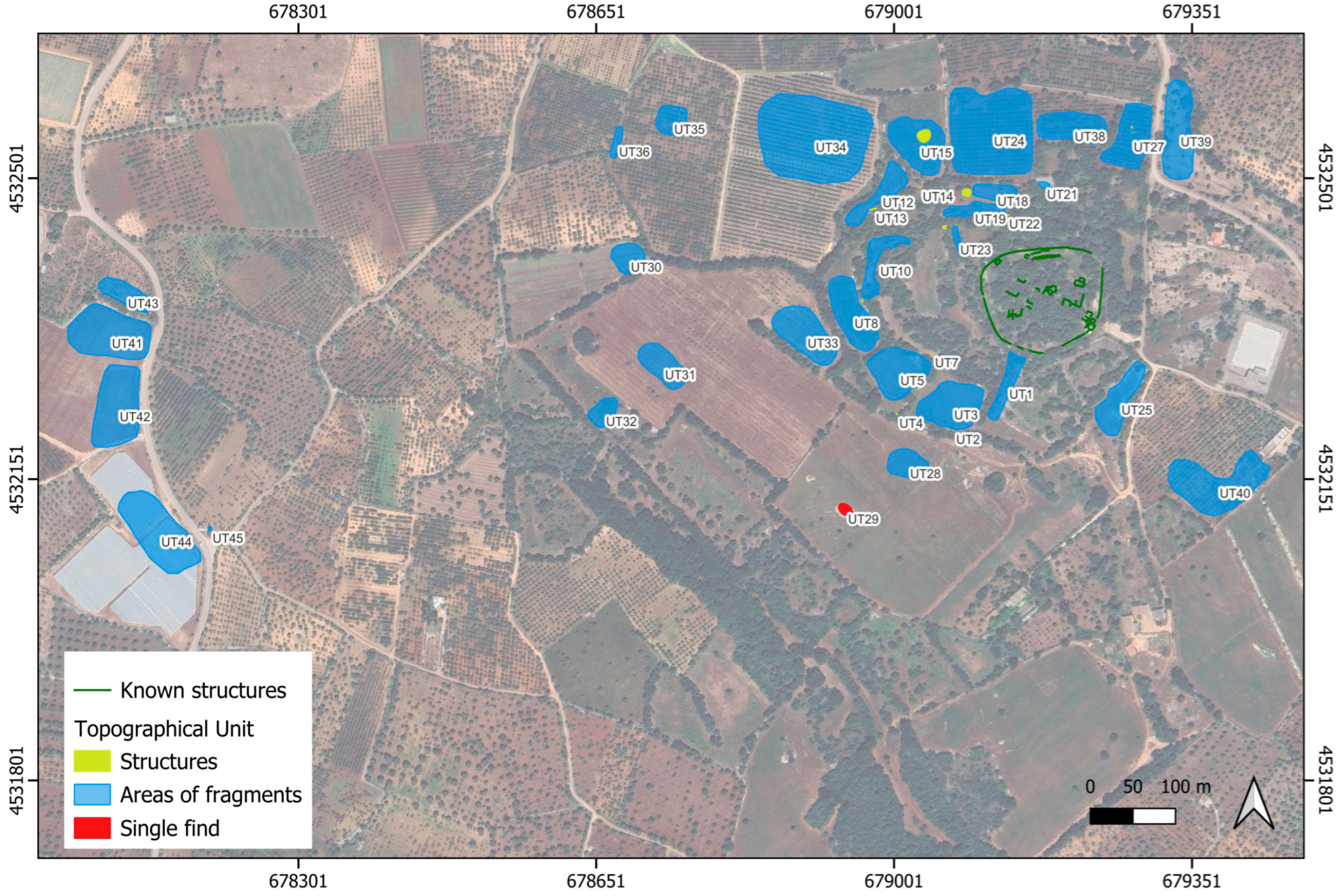
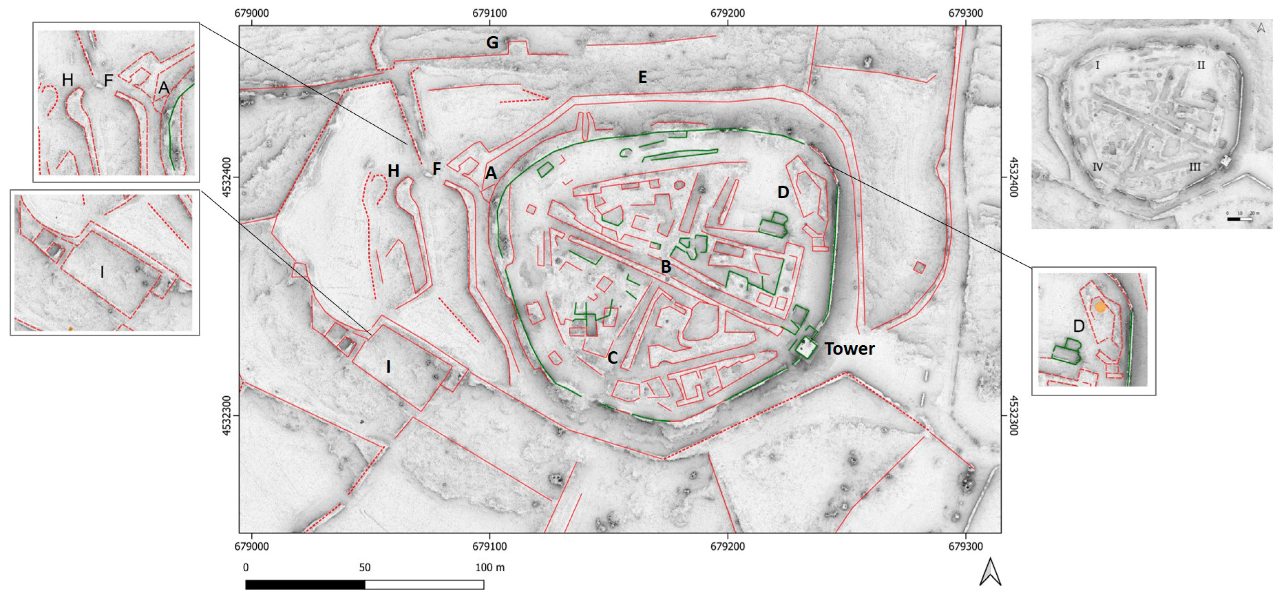
The values described indicate the display and customisation modes of the raster data display offered by QGIS. In particular, brightness, contrast, and saturation can take on either negative or positive values, 0 represents the data as imported, and transparency falls on a 0–100% scale, where 100% represents full visibility of the data.

3. Results

The use of the open-source tool CloudCompare (CC) allowed the segmentation of the entire point cloud obtained from the LiDAR flight using only open-source software and tools. The removal of the outliers and the separation of ground and off-ground points using a CSF filter was quick and easy and resulted in two distinct classes of points. The subsequent manual segmentation of a training sample and the training of the 3DMASC plug-in classifier, all within the framework of CC, allowed the achievement of a simple but effective result. The RF approach applied to segment the ‘off-ground’ point cloud has proven to have great potential to detect useful points for archaeological research (e.g., irregular buildings even below the vegetation or partially present within the ground) from non-useful points (e.g., high vegetation and low vegetation). The statistics of the classifier achieve good results due to the discriminating power of the features calculated on the point cloud before classification, with an overall accuracy estimated by the 3DMASC tool of 0.96 (Figure 5 and

Table 3. Classification statistics.

			Predicted
		Low Veg.	High Veg.	Building	Precision	Recall	F1-Score
	Low Veg.	11,580	2655	230	0.93	0.8	0.86
Real	High Veg.	478	86,665	83	0.96	0.99	0.98
	Building	456	688	9891	0.97	0.9	0.93

).

In Table 3 the rows represent the actual classes (ground truth), while the columns indicate the predictions of the model. The P, R, and F1 scores were calculated in accordance with Formulas (1)–(3).

Observation of the main diagonal shows that the model correctly identifies the following percentages of the samples:

(i)

80.1% of the low vegetation samples,

(ii)

99.4% of the high vegetation samples;

(iii)

89.6% of the building samples.

The process used allowed for a good point cloud segmentation (Figure 6a–c) and for a detailed DTM and DFM creation (Figure 7).

Processing in RVT and in QGIS allowed for a significant improvement in the visibility of natural archaeological features compared to the simple DFM (Figure 8).

The analysis of the produced DFM allowed us to identify several traces connected to architectural structures. These traces were graphically marked, distinguishing them from those already known from previous archaeological excavations and reported in Degano and Zaccaria’s 1981 survey [68]. Some of these alignments were confirmed in the survey data. In the central area of the settlement, a wall perimeter can be distinguished, running roughly circularly. At the south-eastern end, the post-medieval tower is installed, and at the north-western end, a small tower creates a sawtooth with the wall segment (Figure 9A).

Inside the walled area, two parallel alignments oriented northwest–southeast might suggest the existence of a main road, approximately 110 m long (Figure 9B). Such a road is about 4.50 m wide and seems to be bordered by two long parallel walls, each with an average thickness of about 2.60 m. Analyses suggest that his hypothetical road likely connects to another double alignment (93 m long), oriented northeast–southwest, that creates a sort of cardo maximus, particularly visible in the southern portion (Figure 9C). These two main alignments divide the settlement into four quadrants of roughly triangular shape, whose edges appear to be defined by additional traces with an irregular curvilinear path (Figure 9). The church is located in the north-eastern sector (Figure 9II) and it is flanked by the chapel [64,66]. The entrance to the village is located to the east now marked by the 16th-century tower. A residential quarter of irregular layout and today separated from the church is at the north-eastern end (Figure 9D). Moreover, the area is characterised by buildings running parallel to the two main roads mentioned above. Square and rectangular structures are found in all the four sectors. However, the structures more outwards and near the external wall seem to follow the curvilinear trend of the walls themselves. The structures in the south-western sector (Figure 9IV) are poorly preserved and any interpretation is premature at this stage. In the south-east quadrant (Figure 9III) one can recognise a block at the south end, with buildings following a SW-NE trend. At the western end of this perimeter, traces of an articulated structure have been identified, which could represent another defensive element that, together with an east–west wall segment, describes a kind of entrance corridor about 15 m long.

Three of them are in the north-eastern block and one, with a diameter of approximately 4.5 m, is in an isolated position within a kind of irregular enclosure with a north-east/south-west orientation (Figure 10). Only one of these circular shapes can be interpreted, based on the survey data, as a rock-cut shaft (UT 7).

The numerous alignments identified in the vicinity of the village were interpreted as terracing or retaining walls because of their shape. Most of these structures are arranged in circle around the site within the central part of the surveyed area (Figure 10).

Lastly, in the surrounding plain, there are numerous alignments that could indicate the presence of other enclosures protecting cultivated areas. These are a (i) quadrangular structure grafted onto a wall segment to the north (Figure 10A), (ii) a semicircular structure to the west (Figure 10B), and (iii) a double rectangular enclosure to the south-west of the latter (Figure 10C).

4. Discussion

From the analysis of the features of importance and the Confusion Matrix for the classification of LiDAR data in the archaeological context, a clear picture of the model’s capabilities emerges (Figure 6).

The feature importance analysis reveals that the principal components (PCA3, PCA2, PCA1) for larger scales (SC1.6) are among the most influential, suggesting that the finest variation in LiDAR data structure is critical for accurate classification. Other geometric features such as SPHER and PLANA also show a significant growth in importance at an increasing scale. The results obtained support the hypothesis that multiscale analysis techniques are particularly effective in revealing subtle details in LiDAR data and are crucial for the accurate identification of archaeological features. The high precision and recall demonstrate that the model is capable of correctly identifying and classifying archaeological entities in LiDAR data with a low probability of false positives or negatives. The predominance of PCA features at finer scales may indicate that the three-dimensional spatial structure of LiDAR data, contains discriminating information when analysed at finer details. Such information is vital to distinguish between the different types of archaeological artefacts or structures suggesting that pre-processing techniques that preserve or enhance these features could further improve classification [80].

The precision, recall, and F1 score for the identified classes confirm the high model effectiveness, with precision ranging from 92.5% to 96.9%, recall from 80% to 99.3%, and F1 scores from 85.8% to 97.8% (Table 3). Overall, the high vegetation class was particularly well recognised, with a very low error rate (<1%). The low vegetation class, on the other hand, showed 18.4% confusion with the high vegetation class and a residual 1.6% with the building class. The building class was confused with low vegetation in 4.1% of the cases and with high vegetation in 6.2% of the cases.

The data in Table 3 highlights how the high vegetation and building classes are easily distinguishable from each other, above all thanks to the geometric characteristics of the points that compose them. On the contrary, low vegetation is the one that is most easily confused with other classes. This is mainly due to the proximity of the points in this class to those of the other classes, as in the case of bushes or Mediterranean scrub close to tree trunks or structures. Another parameter of misclassification in the discrimination between the archaeological remains and low vegetation could be the geometric “similarity” between the two classes. In fact, the remains of archaeological structures sometimes have a morphology similar to that of low vegetation. However, this problem was solved by using (i) an SOR filter (see Methods) to remove the residuals of low vegetation in the buildings class and (ii) creating DMs at a resolution of 0.2 m/pixel to reduce local noise. According to research on the subject, excessively high resolutions (e.g., 0.02 m/pixel) in the creation of DMs lead to very high local noise phenomena. On the contrary, resolutions from 0.2 to 0.5 m/pixel, depending on the context, provide an excellent information–noise compromise in the field of archaeological research [42,85].

From an archaeological point of view the LiDAR data allowed for the reconstruction of the layout of the medieval village that had previously remained dubious due to the extensive collapse and the thick vegetation covering the entire site. It was possible to confirm the presence of a main east–west roadway [64], defining its extent and measurements. The presence of some buildings along the north-west sector was also confirmed and interpreted as probable workshops. The identification of the traces investigated during the previous archaeological campaigns was also successful. The particular combination of DFM derivatives with the relative parameters allowed to export a detailed plan of the village, increasing our understanding of the function of the 14 previously identified buildings (Figure 11).

5. Conclusions

This paper presents the successful implementation of an open-source approach to process LiDAR data acquired by UAS, applied to a complex archaeological context, with multiple occupation phases, and covered by dense vegetation.

The study allowed the visual obstruction generated by the vegetation to be digitally removed in order to expose areas of the Torre di Castiglione site that are unknown and inaccessible to archaeologists. Knowledge of the site has been expanded with the precise and georeferenced mapping of various structures, paths and roads, defensive structures, towers, and facilities previously unknown. This approach has provided a more precise view of the site, and a new awareness of its boundaries.

The use of a machine learning algorithm (Random Forest) to classify and segment the point clouds revealed previously hidden micro-topographic and structural details, including a main road, residential buildings, defensive walls, and traces of tombs, which were only minimally known until now. Furthermore, it was possible to distinguish these features from those related to the archaeological activities that pertained to the site in the past years. The improved digital models allowed the identification of new archaeological details, increasing the accuracy and interpretation of the site, now entirely covered by vegetation and affected by numerous structural collapses. The generation of high-resolution Digital Feature Models (DFMs) was crucial for the creation of plans revealing complex construction elements and amplifying the understanding of the spatial distribution of the site. The targeted use of visualisation parameters (such as blending modes, brightness, contrast, saturation, and transparency) on DFMs and derivatives ensured exceptional visibility of the archaeological structures, highlighting the importance of the analysis tool customization.

The choice of the open-source software proved effective, demonstrating once again the importance of immediate accessibility of such digital resources to both institutions and independent archaeologists and researchers, and of the replicability of the process. The proposed approach demonstrates that technologies based on advanced algorithms and open-source software can improve the study of archaeological sites, especially those difficult to document, and the efficiency in the employment of the research resources. Probably, solutions based on licences (e.g., GreenValley LiDAR 360 or Blue Marble Global Mapper) or solutions based on deep learning (e.g., Tensorflow or YOLO) exist that can provide superior results to those obtained with 3DMASC. However, this completely open-source approach has proven very useful in the context of a user-friendly point cloud segmentation application, i.e., without the need to use licenced software or complex-programming-language-based systems. This is very important in the context of archaeological and humanities studies, due to the often occurring lack of funds or computer skills. The results encourage further applications of this method, possibly complementing it with other data from remote sensors.

References

1. Küçükdemirci, M.; Landeschi, G.; Ohlsson, M.; Dell’Unto, N. Investigating Ancient Agricultural Field Systems in Sweden from Airborne LIDAR Data by Using Convolutional Neural Network. Archaeol. Prospect. 2022, 30, arp.1886. [Google Scholar] [CrossRef]
2. Lozić, E.; Štular, B. Documentation of Archaeology-Specific Workflow for Airborne LiDAR Data Processing. Geosciences 2021, 11, 26. [Google Scholar] [CrossRef]
3. Štular, B.; Eichert, S.; Lozić, E. Airborne LiDAR Point Cloud Processing for Archaeology. Pipeline and QGIS Toolbox. Remote Sens. 2021, 13, 3225. [Google Scholar] [CrossRef]
4. Štular, B.; Lozić, E.; Eichert, S. Airborne LiDAR-Derived Digital Elevation Model for Archaeology. Remote Sens. 2021, 13, 1855. [Google Scholar] [CrossRef]
5. Lohani, B.; Ghosh, S. Airborne LiDAR Technology: A Review of Data Collection and Processing Systems. Proc. Natl. Acad. Sci. India Sect. A Phys. Sci. 2017, 87, 567–579. [Google Scholar] [CrossRef]
6. Habib, A.F. Airborne Lidar Mapping: Current Status and Future Challenges. Geomatica 2009, 63, 224–226. [Google Scholar] [CrossRef]
7. Krabill, W.; Collins, J.G.; Link, L.; Swift, R.; Butler, M. Airborne Laser Topographic Mapping Results. Photogramm. Eng. Remote Sens. 1984, 50, 685–694. [Google Scholar]
8. Guan, S.; Zhu, Z.; Wang, G. A Review on UAV-Based Remote Sensing Technologies for Construction and Civil Applications. Drones 2022, 6, 117. [Google Scholar] [CrossRef]
9. Wang, R.; Peethambaran, J.; Chen, D. LiDAR Point Clouds to 3-D Urban Models: A Review. IEEE J. Sel. Top. Appl. Earth Obs. Remote Sens. 2018, 11, 606–627. [Google Scholar] [CrossRef]
10. RITCHIE, J.C. Remote Sensing Applications to Hydrology: Airborne Laser Altimeters. Hydrol. Sci. J. 1996, 41, 625–636. [Google Scholar] [CrossRef]
11. Hickman, G.D.; Hogg, J.E. Application of an Airborne Pulsed Laser for near Shore Bathymetric Measurements. Remote Sens. Environ. 1969, 1, 47–58. [Google Scholar] [CrossRef]
12. Mazlan, S.M.; Wan Mohd Jaafar, W.S.; Muhmad Kamarulzaman, A.M.; Saad, S.N.M.; Mohd Ghazali, N.; Adrah, E.; Abdul Maulud, K.N.; Omar, H.; Teh, Y.A.; Dzulkifli, D.; et al. A Review on the Use of LiDAR Remote Sensing for Forest Landscape Restoration. In Concepts and Applications of Remote Sensing in Forestry; Suratman, M.N., Ed.; Springer Nature: Singapore, 2022; pp. 49–74. ISBN 978-981-19419-9-3. [Google Scholar]
13. Stott, D.; Boyd, D.; Beck, A.; Cohn, A. Airborne LiDAR for the Detection of Archaeological Vegetation Marks Using Biomass as a Proxy. Remote Sens. 2015, 7, 1594–1618. [Google Scholar] [CrossRef]
14. Guo, Q.; Su, Y.; Hu, T. LiDAR Principles, Processing and Applications in Forest Ecology; Academic Press: London, UK; San Diego, CA, USA, 2023; ISBN 978-0-12-823894-3. [Google Scholar]
15. Vinci, G.; Vanzani, F.; Fontana, A.; Campana, S. LiDAR Applications in Archaeology: A Systematic Review. Archaeol. Prospect. 2024, 32, arp.1931. [Google Scholar] [CrossRef]
16. Chase, A.F.; Chase, D.Z.; Weishampel, J.F.; Drake, J.B.; Shrestha, R.L.; Slatton, K.C.; Awe, J.J.; Carter, W.E. Airborne LiDAR, Archaeology, and the Ancient Maya Landscape at Caracol, Belize. J. Archaeol. Sci. 2011, 38, 387–398. [Google Scholar] [CrossRef]
17. Doneus, M.; Briese, C.; Fera, M.; Janner, M. Archaeological Prospection of Forested Areas Using Full-Waveform Airborne Laser Scanning. J. Archaeol. Sci. 2008, 35, 882–893. [Google Scholar] [CrossRef]
18. Evans, D.; Traviglia, A. Uncovering Angkor: Integrated Remote Sensing Applications in the Archaeology of Early Cambodia. In Satellite Remote Sensing; Lasaponara, R., Masini, N., Eds.; Remote Sensing and Digital Image Processing; Springer: Dordrecht, The Netherlands, 2012; Volume 16, pp. 197–230. ISBN 978-90-481-8800-0. [Google Scholar]
19. Casana, J.; Laugier, E.J.; Hill, A.C.; Reese, K.M.; Ferwerda, C.; McCoy, M.D.; Ladefoged, T. Exploring Archaeological Landscapes Using Drone-Acquired Lidar: Case Studies from Hawai’i, Colorado, and New Hampshire, USA. J. Archaeol. Sci. Rep. 2021, 39, 103133. [Google Scholar] [CrossRef]
20. Balsi, M.; Esposito, S.; Fallavollita, P.; Melis, M.G.; Milanese, M. Preliminary Archeological Site Survey by UAV-Borne Lidar: A Case Study. Remote Sens. 2021, 13, 332. [Google Scholar] [CrossRef]
21. Chase, A.; Chase, D.; Chase, A. LiDAR for Archaeological Research and the Study of Historical Landscapes. In Geotechnologies and the Environment; Springer: Berlin/Heidelberg, Germany, 2017; pp. 89–100. ISBN 978-3-319-50516-9. [Google Scholar]
22. Chase, A.; Chase, D.; Chase, A. Ethics, New Colonialism, and Lidar Data: A Decade of Lidar in Maya Archaeology. J. Comput. Appl. Archaeol. 2020, 3, 51–62. [Google Scholar] [CrossRef]
23. Devereux, B.J.; Amable, G.S.; Crow, P.; Cliff, A.D. The Potential of Airborne Lidar for Detection of Archaeological Features under Woodland Canopies. Antiquity 2005, 79, 648–660. [Google Scholar] [CrossRef]
24. Canuto, M.A.; Estrada-Belli, F.; Garrison, T.G.; Houston, S.D.; Acuña, M.J.; Kováč, M.; Marken, D.; Nondédéo, P.; Auld-Thomas, L.; Castanet, C.; et al. Ancient Lowland Maya Complexity as Revealed by Airborne Laser Scanning of Northern Guatemala. Science 2018, 361, eaau0137. [Google Scholar] [CrossRef]
25. Rosenswig, R.M.; López-Torrijos, R. Lidar Reveals the Entire Kingdom of Izapa during the First Millennium BC. Antiquity 2018, 92, 1292–1309. [Google Scholar] [CrossRef]
26. Johnson, K.M.; Ouimet, W.B. Rediscovering the Lost Archaeological Landscape of Southern New England Using Airborne Light Detection and Ranging (LiDAR). J. Archaeol. Sci. 2014, 43, 9–20. [Google Scholar] [CrossRef]
27. Masini, N.; Gizzi, F.; Biscione, M.; Fundone, V.; Sedile, M.; Sileo, M.; Pecci, A.; Lacovara, B.; Lasaponara, R. Medieval Archaeology Under the Canopy with LiDAR. The (Re)Discovery of a Medieval Fortified Settlement in Southern Italy. Remote Sens. 2018, 10, 1598. [Google Scholar] [CrossRef]
28. Masini, N.; Lasaponara, R. On the Reuse of Multiscale LiDAR Data to Investigate the Resilience in the Late Medieval Time: The Case Study of Basilicata in South of Italy. J. Archaeol. Method Theory 2021, 28, 1172–1199. [Google Scholar] [CrossRef]
29. Danese, M.; Gioia, D.; Vitale, V.; Abate, N.; Amodio, A.M.; Lasaponara, R.; Masini, N. Pattern Recognition Approach and LiDAR for the Analysis and Mapping of Archaeological Looting: Application to an Etruscan Site. Remote Sens. 2022, 14, 1587. [Google Scholar] [CrossRef]
30. Masini, N.; Abate, N.; Gizzi, F.T.; Vitale, V.; Minervino Amodio, A.; Sileo, M.; Biscione, M.; Lasaponara, R.; Bentivenga, M.; Cavalcante, F. UAV LiDAR Based Approach for the Detection and Interpretation of Archaeological Micro Topography under Canopy—The Rediscovery of Perticara (Basilicata, Italy). Remote Sens. 2022, 14, 6074. [Google Scholar] [CrossRef]
31. Vinci, G.; Bernardini, F. Reconstructing the Protohistoric Landscape of Trieste Karst (North-Eastern Italy) through Airborne LiDAR Remote Sensing. J. Archaeol. Sci. Rep. 2017, 12, 591–600. [Google Scholar] [CrossRef]
32. Ladefoged, T.N.; McCoy, M.D.; Asner, G.P.; Kirch, P.V.; Puleston, C.O.; Chadwick, O.A.; Vitousek, P.M. Agricultural Potential and Actualized Development in Hawai’i: An Airborne LiDAR Survey of the Leeward Kohala Field System (Hawai’i Island). J. Archaeol. Sci. 2011, 38, 3605–3619. [Google Scholar] [CrossRef]
33. Snitker, G.; Moser, J.D.; Southerlin, B.; Stewart, C. Detecting Historic Tar Kilns and Tar Production Sites Using High-Resolution, Aerial LiDAR-Derived Digital Elevation Models: Introducing the Tar Kiln Feature Detection Workflow (TKFD) Using Open-Access R and FIJI Software. J. Archaeol. Sci. Rep. 2022, 41, 103340. [Google Scholar] [CrossRef]
34. Raab, A.; Schneider, A.; Bonhage, A.; Raab, T. Charcoal Burning—A Neglected Soil-Forming Factor in Cultural Landscapes. 2024. Available online: https://www.researchgate.net/publication/380912290_CHARCOAL_BURNING_-_A_NEGLECTED_SOIL-FORMING_FACTOR_IN_CULTURAL_LANDSCAPES (accessed on 10 December 2024).
35. Renfrew, C.; Bahn, P.G. Archaeology: Theories, Methods, and Practice; Seventh Edition Revised & Updated; Thames & Hudson: London, UK, 2016; ISBN 978-0-500-29210-5. [Google Scholar]
36. Forte, M.; Campana, S.R.L. (Eds.) Digital Methods and Remote Sensing in Archaeology: Archaeology in the Age of Sensing; Quantitative Methods in the Humanities and Social Sciences; Springer International Publishing: Berlin/Heidelberg, Germany, 2016; ISBN 978-3-319-40656-5. [Google Scholar]
37. Khan, S.; Aragão, L.; Iriarte, J. A UAV–Lidar System to Map Amazonian Rainforest and Its Ancient Landscape Transformations. Int. J. Remote Sens. 2017, 38, 2313–2330. [Google Scholar] [CrossRef]
38. Evans, D. Airborne Laser Scanning as a Method for Exploring Long-Term Socio-Ecological Dynamics in Cambodia. J. Archaeol. Sci. 2016, 74, 164–175. [Google Scholar] [CrossRef]
39. Parcero-Oubiña, C.; Nión, S. At Last! Remote-Sensing Discovery of Archaeological Features Through Aerial Imagery and Lidar in Galician Hillforts. 2021. Available online: https://digital.csic.es/handle/10261/268425 (accessed on 10 December 2024).
40. Parcero-Oubiña, C. At Last! Discovery of Archaeological Features Through Aerial Imagery and Lidar at Galician Hillforts. 2022. Available online: https://digital.csic.es/handle/10261/305526 (accessed on 10 December 2024).
41. Bollandsås, O.; Risbøl, O.; Ene, L.; Nesbakken, A.; Gobakken, T.; Næsset, E. Using Airborne Small-Footprint Laser Scanner Data for Detection of Cultural Remains in Forests: An Experimental Study of the Effects of Pulse Density and DTM Smoothing. J. Archaeol. Sci. 2012, 39, 2733–2743. [Google Scholar] [CrossRef]
42. Mazzacca, G.; Grilli, E.; Cirigliano, G.P.; Remondino, F.; Campana, S. Seeing among foliage with lidar and machine learning: Towards a transferable archaeological pipeline. Int. Arch. Photogramm. Remote Sens. Spat. Inf. Sci. 2022, XLVI-2/W1-2022, 365–372. [Google Scholar] [CrossRef]
43. Campana, S. Drones in Archaeology. State-of-the-Art and Future Perspectives: Drones in Archaeology. Archaeol. Prospect. 2017, 24, 275–296. [Google Scholar] [CrossRef]
44. Sánchez, J.G. Archaeological LiDAR in Italy: Enhancing Research with Publicly Accessible Data. Antiquity 2018, 92, e4. [Google Scholar] [CrossRef]
45. Fiorucci, M.; Khoroshiltseva, M.; Pontil, M.; Traviglia, A.; Del Bue, A.; James, S. Machine Learning for Cultural Heritage: A Survey. Pattern Recognit. Lett. 2020, 133, 102–108. [Google Scholar] [CrossRef]
46. Guyot, A.; Lennon, M.; Lorho, T.; Hubert-Moy, L. Combined Detection and Segmentation of Archeological Structures from LiDAR Data Using a Deep Learning Approach. J. Comput. Appl. Archaeol. 2021, 4, 1. [Google Scholar] [CrossRef]
47. Richards-Rissetto, H.; Newton, D.; Al Zadjali, A. A 3D point cloud deep learning approach using lidar to identify ancient maya archaeological sites. ISPRS Ann. Photogramm. Remote Sens. Spat. Inf. Sci. 2021, VIII-M-1–2021, 133–139. [Google Scholar] [CrossRef]
48. Trotter, E.; Fernandes, A.; Fibæk, C.; Keßler, C. Machine Learning for Automatic Detection of Historic Stone Walls Using LiDAR Data. Int. J. Remote Sens. 2022, 43, 2185–2211. [Google Scholar] [CrossRef]
49. Briese, C.; Pfeifer, N. Airborne Laser Scanning and Derivation of Digital Terrain Models. In Proceedings of the 5th Conference on Optical 3D Measurement Techniques, Vienna, Austria, 1–4 October 2001; pp. 80–87. [Google Scholar]
50. Inomata, T. Lidar, Space, and Time in Archaeology: Promises and Challenges. Annu. Rev. Anthropol. 2024, 53, 75–92. [Google Scholar] [CrossRef]
51. Doneus, M.; Briese, C. Full-Waveform Airborne Laser Scanning as a Tool for Archaeological Reconnaissance. In From Space to Place; Archeopress: Oxford, UK, 2015; pp. 99–106. [Google Scholar]
52. Buján, S.; Cordero, M.; Miranda, D. Hybrid Overlap Filter for LiDAR Point Clouds Using Free Software. Remote Sens. 2020, 12, 1051. [Google Scholar] [CrossRef]
53. Pfeifer, N.; Mandlburger, G. Lidar Data Filtering and Digital Terrain Model Generation; CRC Press: Boca Raton, FL, USA, 2018; pp. 349–378. [Google Scholar]
54. Štular, B.; Lozić, E. Comparison of Filters for Archaeology-Specific Ground Extraction from Airborne LiDAR Point Clouds. Remote Sens. 2020, 12, 3025. [Google Scholar] [CrossRef]
55. Suleymanoglu, B.; Soycan, M. Comparison of Filtering Algorithms Used for DTM Production from Airborne Lidar Data: A Case Study in Bergama, Turkey. Geod. Vestn. 2019, 63, 395–414. [Google Scholar] [CrossRef]
56. Kokalj, Ž.; Zakšek, K.; Oštir, K.; Pehani, P.; Čotar, K.; Somrak, M. Relief Visualization Toolbox, Ver. 2.2.1 Manual. Remote Sens. 2016, 3, 398–415. [Google Scholar]
57. Zakšek, K.; Oštir, K.; Kokalj, Ž. Sky-View Factor as a Relief Visualization Technique. Remote Sens. 2011, 3, 398–415. [Google Scholar] [CrossRef]
58. Kokalj, Ž.; Somrak, M. Why Not a Single Image? Combining Visualizations to Facilitate Fieldwork and On-Screen Mapping. Remote Sens. 2019, 11, 747. [Google Scholar] [CrossRef]
59. Miroslav Marin, M. Torre Di Castiglione 1. La Campagna Topografica Del 1981; Grafica Bigiemme: Bari, Italy, 1985; Volume 1. [Google Scholar]
60. Caprio, A. Il Megalitismo in Area Italica: Le Mura Antiche Di Conversano e Di Castiglione. Stor. E Cult. Terra Bari 2010, V, 9–14. [Google Scholar]
61. Caprio, A. Castiglione. Gli Scavi Degli Anni 1986-87 e 1997. In Norba-Conversano. Archeologia e Storia Della Città e Del Territorio; Adda: Bari, Italy, 2013; pp. 457–478. [Google Scholar]
62. Ciancio, A. Il Sito Di Castiglione Tra Conoscenza e Valorizzazione. In Una Finestra Sulla Storia. Un Cavaliere a Castiglione Tra Angioini e Aragonesi; Edizioni Storia Patria: Conversano, Italy, 2017; pp. 22–27. [Google Scholar]
63. Caprio, A. Origine e Fine Del Villaggio Rurale Di Castiglione (Conversano). Stor. E Cult. Terra Bari Studi E Ric. 2015, VI, 21–31. [Google Scholar]
64. Caprio, A. La Storia Del Casale Attraverso i Dati Della Ricerca Archeologica. In Una Finestra Sulla Storia. Un Cavaliere a Castiglione Tra Angioini e Aragonesi; Edizioni Storia Patria: Conversano, Italy, 2017; pp. 28–36. [Google Scholar]
65. Fanizzi, A. Castiglione Nei Documenti. In Una Finestra Sulla Storia. Un Cavaliere a Castiglione Tra Angioini e Aragonesi; Edizioni Storia Patria: Conversano, Italy, 2017; pp. 62–72. [Google Scholar]
66. Perfido, P. Castiglione: Un Villaggio Fortificato Di Fondazione Angioina. In Una Finestra Sulla Storia. Un Cavaliere a Castiglione Tra Angioini e Aragonesi; Edizioni Storia Patria: Conversano, Italy, 2017; pp. 37–55. [Google Scholar]
67. L’Abbate, V. Dalla ‘Scoperta’ Ottocentesca Alle Indagini Del XX Secolo. In Norba-Conversano. Archeologia e Storia Della Città e Del Territorio; Adda: Bari, Italy, 2013; pp. 437–448. [Google Scholar]
68. Degano, E.; Zaccaria, C. Rappresentazioni Cartografiche e Grafiche. In Torre di Castiglione 1. La Campagna Topografica Del 1981; Società di Storia Patria per la Puglia: Bari, Italy, 1985; Volume 5, pp. 39–40. [Google Scholar]
69. Adams, R.; Wood, E. Ancient Maya Canals: Grids and Lattices in the Maya Jungle. Archaeology 1982, 35, 28–35. [Google Scholar]
70. Banaszek, Ł. LiDARchaeology. Airborne Laser Scanning of the Forested Landscapes around Polanów (Pomerania, Poland). In Aerial Archaeology and Remote Sensing from the Baltic to the Adriatic; Eotvos Lorand University: Budapest, Hungary, 2013; pp. 31–36. [Google Scholar]
71. Fernandez-Diaz, J.; Carter, W.; Shrestha, R.; Glennie, C. Now You See It… Now You Don’t: Understanding Airborne Mapping LiDAR Collection and Data Product Generation for Archaeological Research in Mesoamerica. Remote Sens. 2014, 6, 9951–10001. [Google Scholar] [CrossRef]
72. Opreanu, C.; Lăzărescu, V.; Roman, A.; Ursu, T.; Farcas, S. New Light on a Roman Fort Based on a LiDAR Survey in the Forested Landscape from Porolissvm. Ephemer. Napoc. 2014, 24, 71–86. [Google Scholar]
73. Roussel, J.-R.; Auty, D.; Coops, N.C.; Tompalski, P.; Goodbody, T.R.H.; Meador, A.S.; Bourdon, J.-F.; de Boissieu, F.; Achim, A. lidR: An R Package for Analysis of Airborne Laser Scanning (ALS) Data. Remote Sens. Environ. 2020, 251, 112061. [Google Scholar] [CrossRef]
74. Breiman, L. Random Forests. Mach. Learn. 2001, 45, 5–32. [Google Scholar] [CrossRef]
75. Corcoran, J.; Knight, J.; Pelletier, K.; Rampi, L.; Wang, Y. The Effects of Point or Polygon Based Training Data on RandomForest Classification Accuracy of Wetlands. Remote Sens. 2015, 7, 4002–4025. [Google Scholar] [CrossRef]
76. Letard, M.; Lague, D.; Le Guennec, A.; Lefèvre, S.; Feldmann, B.; Leroy, P.; Girardeau-Montaut, D.; Corpetti, T. 3DMASC: Accessible, Explainable 3D Point Clouds Classification. Application to BI-Spectral TOPO-Bathymetric Lidar Data. ISPRS J. Photogramm. Remote Sens. 2024, 207, 175–197. [Google Scholar] [CrossRef]
77. Brodu, N.; Lague, D. 3D Terrestrial Lidar Data Classification of Complex Natural Scenes Using a Multi-Scale Dimensionality Criterion: Applications in Geomorphology. ISPRS J. Photogramm. Remote Sens. 2012, 68, 121–134. [Google Scholar] [CrossRef]
78. Hackel, T.; Wegner, J.D.; Schindler, K. Fast semantic segmentation of 3D point clouds with strongly varying density. ISPRS Ann. Photogramm. Remote Sens. Spat. Inf. Sci. 2016, III–3, 177–184. [Google Scholar] [CrossRef]
79. Blomley, R.; Jutzi, B.; Weinmann, M. 3D Semantic Labeling of ALS Point Clouds by Exploiting Multi-Scale, Multi-Type Neighborhoods for Feature Extraction. 2016. Available online: https://www.researchgate.net/publication/312948032_3D_semantic_labeling_of_ALS_point_clouds_by_exploiting_multi-scale_multi-type_neighborhoods_for_feature_extraction (accessed on 10 December 2024).
80. Tarsha Kurdi, F.; Amakhchan, W.; Gharineiat, Z.; Boulaassal, H.; El Kharki, O. Contribution of Geometric Feature Analysis for Deep Learning Classification Algorithms of Urban LiDAR Data. Sensors 2023, 23, 7360. [Google Scholar] [CrossRef]
81. Kokalj, Ž.; Hesse, R. Airborne Laser Scanning Raster Data Visualization; Prostor, kraj, čas; ZRC SAZU, Založba ZRC: Ljubljana, Slovenia, 2017; Volume 14, ISBN 978-961-254-984-8. [Google Scholar]
82. Vianello, A.; Cavalli, M.; Tarolli, P. LiDAR-Derived Slopes for Headwater Channel Network Analysis. CATENA 2009, 76, 97–106. [Google Scholar] [CrossRef]
83. Hesse, R. LiDAR-derived Local Relief Models—A New Tool for Archaeological Prospection. Archaeol. Prospect. 2010, 17, 67–72. [Google Scholar] [CrossRef]
84. Toumazet, J.P.; Simon, F.-X.; Mayoral, A. Self-AdaptIve LOcal Relief Enhancer (SAILORE): A New Filter to Improve Local Relief Model Performances According to Local Topography. Geomatics 2021, 1, 450–463. [Google Scholar] [CrossRef]
85. Doneus, M. Openness as Visualization Technique for Interpretative Mapping of Airborne Lidar Derived Digital Terrain Models. Remote Sens. 2013, 5, 6427–6442. [Google Scholar] [CrossRef]
86. Lasaponara, R.; Masini, N. Full-Waveform Airborne Laser Scanning for the Detection of Medieval Archaeological Microtopographic Relief. J. Cult. Herit. 2009, 10, e78–e82. [Google Scholar] [CrossRef]
Figure 1. Study area location.
Remotesensing 17 01134 g001
Figure 2. Maps with known structures and UT from previous excavation and survey.
Remotesensing 17 01134 g002
Figure 3. Operational flowchart.
Remotesensing 17 01134 g003
Figure 4. Point density map points per m2 obtained using lidR (4.1.2) in Rstudio (v.12.1) [73].
Remotesensing 17 01134 g004
Figure 5. Weight of the calculated features (Table 1) at different scales during the classification process: (a) the importance of features; (b) the importance of features per type; (c) the importance of the scale of calculated features.
Remotesensing 17 01134 g005
Figure 6. Point clouds (left) top view and (right) bird’s eye view. (a) Original point cloud; (b) result of CSF filtering to extract the ground point; (c) classified point cloud.
Remotesensing 17 01134 g006
Figure 7. (a) DSM and (b) DFM at resolution of 0.2 m/pixel.
Remotesensing 17 01134 g007
Figure 8. (a) HS; (b) MHS; (c) PCAHS; (d) slope; (e) SLRM; (f) SVF; (g) OP; (h) ON; (i) LD; (j) MSRM; (k) MSTP; (l) VAT; (m) image fusion operation No. 1; (n) image fusion operation No. 2; (o) image fusion operation No. 3.
Remotesensing 17 01134 g008
Figure 9. The centre of the Torre Castiglione site with evidence of the archaeological traces identified by LiDAR (red) and those already known (green); the images on the left and right zoom in on the areas described in the text.
Remotesensing 17 01134 g009
Figure 10. Archaeological map resulting from LiDAR analysis (red) and previous surveys (green), including UTs (territorial units).
Remotesensing 17 01134 g010
Figure 11. Map of the Torre Castiglione site with an interpretation of the highlighted traces and subdivision based on the type of evidence (from excavation/survey, geophysical survey, or LIDAR).
Remotesensing 17 01134 g011