Assessing the Impact of Land Use Changes on Ecosystem Service Values in Coal Mining Regions Using Google Earth Engine Classification

Abstract

Understanding the impacts of land use and land cover changes on ecosystem service values (ESVs) is crucial for effective ecosystem management; however, the intricate relationship between these factors in coal mining regions remains underexplored. In particular, the influence of coal mining activities on these dynamics is insufficiently understood, leaving a gap in the literature that hinders the development of robust management strategies. To address this gap, we investigated the interplay between land use change and the ESV at the interface of Yang Coal Mine No. 2 and the Shanxi Yalinji Guanshan Provincial Nature Reserve in Yangquan City, Shanxi Province. Using Landsat 8 remote sensing data from 2013 to 2021, our approach incorporated analyses using the Google Earth Engine (GEE) platform. We employed a random forest algorithm to classify land use patterns and calculated key indices—including the normalized difference vegetation index (NDVI), normalized difference built-up index (NDBI), enhanced vegetation index (EVI), and bare soil index (BSI)—which were combined with topographic features. Land use change dynamics were quantified via a transfer matrix, while changes in the ESV were evaluated using the ecosystem sensitivity index and ecological contribution rate. Our results revealed notable fluctuations: forestland increased from 2013 to 2018 before declining sharply from 2019 to 2021; grassland displayed similar variability; and constructed land experienced a continual expansion. Correspondingly, the overall ESV increased by 28.6% from 2013 to 2019, followed by a 19.5% decline in 2020 and 2021, with forest and grassland’s ESVs exhibiting similar trends. These findings demonstrate that land use changes, particularly those that are driven by human activities such as coal mining, have a significant impact on ecosystem service values in mining regions. By unraveling the nuanced relationship between land use dynamics and ESVs, our study not only fills the gap in the literature but also provides valuable insights for developing more effective ecosystem management strategies, ultimately advancing our understanding of ecosystem dynamics in human-impacted landscapes.

1. Introduction

Coal, as one of the principal global energy sources, has historically been a fundamental driver of both global economic expansion and societal development [1]. However, ecological and environmental issues caused by coal mining activities, such as surface subsidence, vegetation degradation, soil erosion, and water pollution, have become an escalating global concern [2]. These issues not only damage the ecological environment of mining areas but also threaten the ecological security and sustainable development in surrounding regions, potentially impacted by processes such as soil erosion and climate change [3,4,5]. This situation becomes even more complex in areas where coal mining overlaps with nature reserves, as the ecological vulnerability is heightened, and the impacts on ecosystem services (ESs) are more profound and intricate [6].

Coal mining regions are often situated in ecologically sensitive areas, where significant land use changes occur rapidly, leading to alterations in ecosystem functions and services [7,8,9]. In this context, studying ecological changes in coal mining areas is essential. Particularly in regions where coal mining overlaps with nature reserves, balancing mining with ecological conservation and the sustainability of ecosystem services presents an urgent issue that must be addressed [4,5,10]. Research in these regions helps systematically determine the far-reaching impacts of coal mining on the ecological environment, providing scientific evidence and theoretical support for integrating resource development and ecological protection [11].

In mining area studies, comparing standardized equivalence coefficients with the unique land use characteristics reveals that even in the presence of ecological disturbances, appropriately adjusted coefficients can effectively represent the overall level of ecosystem services. This method has been validated across several regions, demonstrating reliable comparability and generalizability and proving useful for assessing ecosystem services following land use changes [12]. However, ecosystem restoration and shifts in land use within mining areas often exhibit pronounced spatial and temporal dynamics [13]. As a static assessment tool, the traditional equivalent coefficient method struggles to fully capture these evolving changes. Therefore, this study further incorporates a dynamic assessment model to improve the spatio-temporal adaptability and accuracy of ecological service assessments.

Costanza et al., (1997) pioneered the area of systematic assessment of global ecosystem service values using a unit area valuation methodology [14]. Building on these insights, Xie et al., (2003) implemented the method developed by Costanza to quantitatively evaluate the values of ecosystem services in a Chinese region [15,16,17,18]. Since the 1980s, there has been a growing interest among researchers in studying ecosystem service values in relation to land use changes. These studies focus on how land use changes impact ecosystem service values within specific regions. In this context, Qian et al., (2018) conducted a trade-off analysis of mining benefits versus ESV losses on the southern slopes of the Qilian Mountains to understand the impact of mining on land and ecosystem services [19]. Further advancements in this methodology were demonstrated by Quan et al., (2024), who used an improved satellite remote sensing equivalence factor valuation approach to compute the ESV of Anhui Province over the past 30 years [20]. They analyzed the spatial and temporal evolution of the ESV and investigated the driving mechanisms behind these changes. They also used the GeoSOS-FLUS model to predict the ESV of Anhui Province by 2030. Zhang et al., (2024) studied the effects of land use changes on the ESV in the Hexi region from 1990 to 2020 using the improved Equivalent Factor Approach. They highlighted the importance of ESV changes for the harmonious development of the ecological environment and human society [21]. Qian et al., (2020) examined the balance between mineral resource mining in ecologically fragile areas and the ecological environment [22]. This study monitored land use changes in the mining range and surrounding land from 1975 to 2016 in the Qinghai–Tibetan Plateau mining areas, considering spatial adjacency effects. It compared the economic gains from mine development with the increases and decreases in the ESV, emphasizing the complex interplay between resource extraction and ESVs. Currently, a growing number of studies focus on the impacts of land use changes on ecosystem service values (ESVs). The existing research generally concentrates on how different land use changes, including agricultural expansion, urbanization, and mining activities, influence ecosystem services [23]. Common findings indicate that land use change is the primary driver of fluctuations in ESVs, particularly in areas with intensive human activities, where the relationship between land use changes and ecosystem service value fluctuations is especially strong.

The existing research has several gaps: First, a limited number of studies have examined the overlapping areas of coal mining and nature reserves, neglecting the complex interactions between land use changes and ecosystem services in these regions. Second, most studies offer static assessments, lacking a systematic analysis of the long-term impacts of dynamic land use changes on ESVs. Additionally, advanced tools such as Google Earth Engine (GEE) remain underutilized, restricting the efficiency and precision of ESV evaluations. Addressing these gaps is crucial for advancing our understanding of the impact of land use on ecosystem services in coal mining regions, especially those overlapping with protected areas.

This study begins by applying the random forest algorithm to identify and classify land use types. Random forest is an efficient machine learning method that can handle high-dimensional data with high classification accuracy, making it widely used in land use classifications of remote sensing images [24]. After classification, land use transition matrices and dynamic change analysis are applied to quantitatively describe the directional changes and transformation patterns of land use types over different time periods, revealing trends in land use changes and providing the foundational data that are required for further assessing the impact of such changes on the ESV.

Building on earlier findings, this study further examined the connection between land use changes and ESVs. To quantify this relationship, a sensitivity analysis was performed, focusing on how alterations in land use affect ecosystem services [25]. Two key indicators were employed: the ecological sensitivity index and the ecological contribution ratio. The sensitivity index evaluates how ecosystems respond to natural variations and human disturbances—reflecting the regional vulnerability—while the contribution ratio measures the added value of different land use types, highlighting their impact on ecological benefits [26]. Recent research, both domestically and internationally, has moved from addressing individual ecological issues to examining these indicators together [27]. This comprehensive approach aims to develop a robust theoretical framework for regional environmental management and sustainable development, while also clarifying how changes in land use impact ecosystem services.

Finally, through an ecological contribution rate analysis, this study evaluates the contribution of different land use types to the overall change in the ESV. By quantifying the contribution rates of various land use types, the analysis identifies which land use types play a dominant role in ecosystem services and further clarifies how different land use types drive the functions of ecosystem services. The results of this analysis will provide a scientific basis for optimizing ecological protection strategies, increasing the efficiency of resource management, and promoting regional sustainable development.

2. Materials and Methods

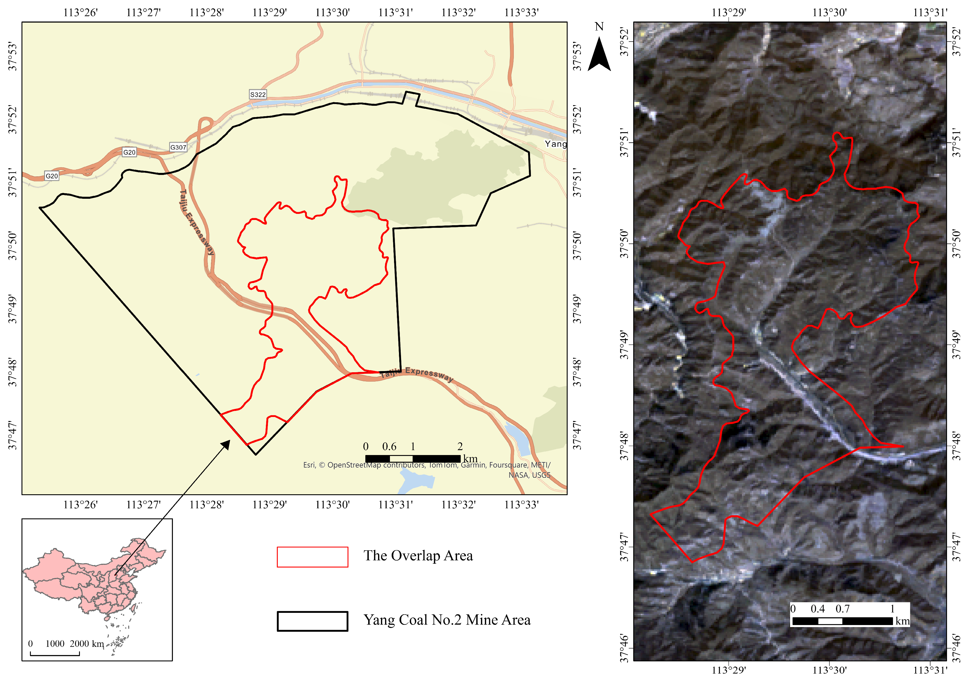
2.1. Study Area

Yang Coal Mine No. 2 (YME), established on 1 May 1951, is a subsidiary of Yang Coal Group. Located at the western foot of Taihang Mountain, it covers an area of 60.0603 km², with an annual production capacity of 4 million tons. The depth of the mine ranges from 463.3 m to 713.5 m. Its shaft field extends across three regions: the suburbs of Yangquan City, the mining area, and Pingding County. Situated approximately 5 km from Yangquan City, the mine is located at geographic coordinates ranging from 113°25′17″ to 113°33′07″ eastern longitude and 37°46′44″ to 37°52′19″ northern latitude [28,29]. The well field is positioned in the mid-to-high mountainous area of the Loess Plateau in Shanxi, characterized by a steep terrain, longitudinal gullies, valleys, and significant variations in topographic elevation. The Shanxi Yalin Temple Crown Mountain Provincial Nature Reserve is situated in the Taihang Mountain region of eastern Shanxi Province. It encompasses an area of 110.17 km² that includes both the Qiulin and Yalin Temple districts. In 2002, the establishment of the reserve led to an overlap between the mining area of Yang Coal Mine No. 2 and the reserve boundaries, thereby creating a zone designated for special management with significant ecological importance. This overlap encompasses approximately 13.995 km², with the air-mining zone covering about 4.742 km², as shown in Figure 1. Given that the development of the 15# coal mining area of YME occurred after the establishment of the nature reserve, the operations conducted between 2004 and 2016 contravened Article 18, as well as Articles 26–29 and 32, of the Regulations of the People’s Republic of China on the nature reserve. Following the issuance of the directive “Yanglin Bin Zi [2017] No. 27”, which prohibits coal mining within the study area and Lion Brain Mountain Forest Park, mining operations in the overlapping zone (defined as the area within 500 m of the outer boundary of the nature reserve) were completely halted. Additionally, substantial manpower, resources, and expert research have been dedicated to assessing and mitigating the ecological and environmental impacts on the nature reserve.

2.2. Data Preparation

Google Earth Engine (GEE) is a powerful cloud computing platform, introduced by Google Inc. in 2010 [30,31]. It excels in data acquisition, analysis, and processing. Compared with traditional remote sensing image processing software such as ENVI 5.3 and ArcGIS 10.8, GEE offers distinct advantages [32]. The platform provides numerous open sources, including public datasets and free storage space. It integrates datasets from multiple satellite platforms, including Landsat, MODIS, Sentinel, SRTM, DMSP, and NPP VIIRS, totaling over 200 datasets. These features make GEE an essential tool for remote sensing image processing [33].

This study primarily utilized Landsat 8 remote sensing imagery provided by the USGS, covering the overlapping area of YME from 2013 to 2021. We processed all Landsat imagery, obtained using the Landsat (SR) sensor, directly on the GEE platform.

Landsat 8 satellite data are indispensable for regional land cover classification due to their high spatial resolution and consistent data availability. Most sensors capture images at a 30 m resolution—15 m for panchromatic bands—meaning that each pixel represents roughly 900 square meters [34]. For a study area of 13.995 km² (approximately 13,995,000 square meters), this equates to about 15,550 pixels, ensuring that even subtle changes in landscape features and environmental conditions are well documented [35]. This resolution reliably differentiates major surface elements such as urban areas, farmland, forests, and water bodies [36]. Moreover, the free and continuous availability of Landsat 8 data, combined with their rich multispectral capabilities, provides a robust basis for monitoring and analyzing environmental changes over time [37]. Landsat’s comprehensive datasets not only support detailed spatial assessments but also support temporal studies, which are essential for understanding land use dynamics and guiding informed decision-making in environmental research.

The processing involved several steps: First, we selected all surface reflectance (SR) data for each study year during the vegetation’s growing season (1 May to 30 September). 1 May to 30 September corresponds to the primary growing season for vegetation, especially in the Northern Hemisphere [38,39,40]. During this period, vegetation grows vigorously and is significantly influenced by climatic conditions, making it a more reliable indicator of the effects of land use changes on vegetation cover in a region [41,42]. During this period, temperatures rise gradually, rainfall is abundant, and vegetation grows actively, which makes NDVI images highly sensitive to changes in vegetation cover, thus effectively capturing changes caused by land use [43,44,45]. Additionally, satellite remote sensing imagery offers a high spatial resolution, enabling precise monitoring of the vegetation cover [46,47,48]. The NDVI is a commonly used index for assessing vegetation cover, and its sensitivity to reflectance changes is heightened, particularly during the growing season [49,50]. Therefore, selecting imagery from this period enhances the accuracy and sensitivity of classification. For instance, NDVI values typically reach their highest annual values during this period, and the changes in vegetation reflectance are more pronounced, thereby providing a clearer indication of the ecosystem’s condition and any changes [51].

To effectively remove cloud interference and noise, smooth the time series data, improve the image quality, preserve feature details, and ensure compatibility with data synthesis across different time scales, we used the pixel_qa band from Landsat 8, which contains pixel quality information, and performed cloud removal using the “maskL8sr” function. We then used the median function in GEE to generate a composite image from the filtered set. Finally, we calculated the normalized difference vegetation index (NDVI), normalized difference built-up index (NDBI), enhanced vegetation index (EVI), and bare soil index (BSI) for each image. The NDVI and EVI effectively highlight the vegetation distribution and intensity, the BSI enhances bare soil elements, while the NDBI primarily highlights built-up areas [52]. The final result is the best cloud-free image combination incorporating the NDVI, NDBI, EVI, and BSI. Additionally, this study used SRTM DEM data provided by the GEE platform as the primary auxiliary data for extracting terrain features.

For data sources, this study reviewed planted area and grain production data from the Shanxi Provincial Statistical Yearbook and visited the website of the State Bureau of Grain and Material Reserves (lswz.gov.cn), which contains the required grain price data for the study. Land use classification for the study area was carried out based on the “Land Use Classification” standard (GB/T 21010-2017) [53]. Lastly, this study obtained data on vegetation types and the current state of the study area from the “Comprehensive Environmental Impact Report of Yaolin Temple Guanshan Nature Reserve in the Yang Coal Mine No. 2 Mining Area”.

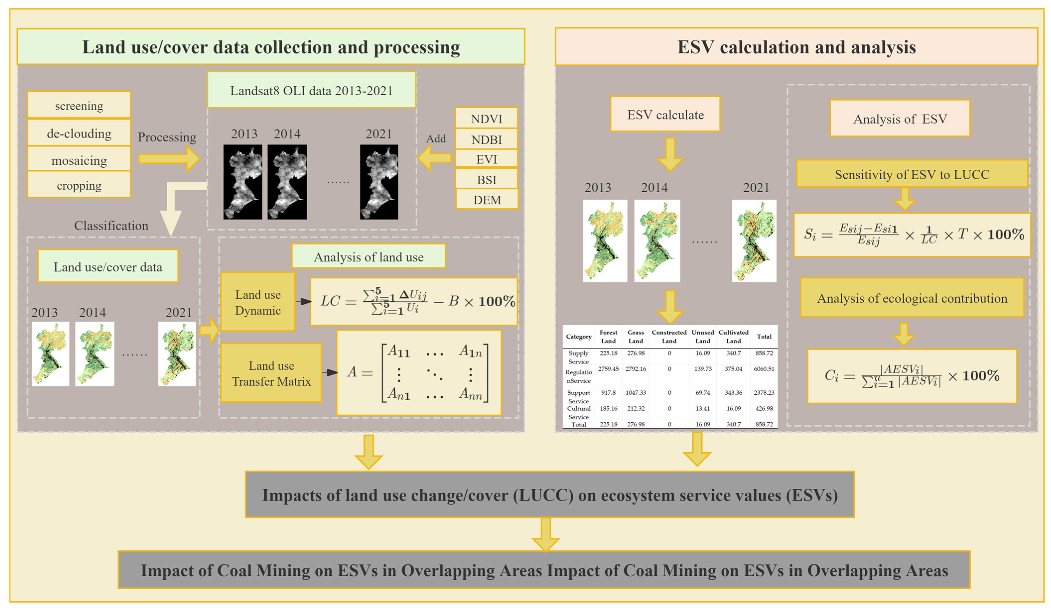
2.3. Technological Processes

The specific process comprised eight distinct steps, as visually depicted in Figure 2.

In this study, we utilized the Google Earth Engine (GEE) cloud platform to acquire Landsat 8 satellite images (a total of nine images, one per year) from 2013 to 2021 for analysis. First, we selected images before and after the coal mine was shut down in 2018 and then preprocessed these images through filtering, de-clouding, mosaicking, and cropping to ensure high quality and clarity and that the images were free from clouds for subsequent analysis. Using the Land Use Classification standard (GB/T 21010-2017) and the actual land cover of the overlap area, we categorized the land use types into five classes: forestland, grassland, constructed land, unused land, and cultivated land. To perform the classification, we randomly selected 70 sample points from the study area through visual interpretation on the GEE platform and applied the random forest algorithm. To prevent model overfitting, we set the number of trees in the model to 50.

To improve the classification accuracy and Kappa coefficients, ensuring that they met our precision requirements, this study selected multiple spectral and topographic features for classification, including spectral indices such as the NDBI, NDVI, BSI, and EVI, as well as topographic indices such as elevation. The classification accuracy was assessed using a confusion matrix, and the sample data were randomly divided into a training set (70%) and a testing set (30%).

Subsequently, we calculated the land use dynamics and land use transition matrix to quantitatively describe the direction and extent of land use type conversions, revealing trends in land use changes. Meanwhile, using the ecosystem sensitivity index, we assessed the sensitivity of the ecosystem service value (ESV) to land use changes. Finally, the ecological contribution rate analysis further explored the primary factors contributing to ESV changes, providing scientific evidence for subsequent ecological conservation and land management.

2.4. Methods

2.4.1. Land Use Classification Based on Random Forest Algorithm and GEE Platform

Compared with traditional classification algorithms, the random forest algorithm is notable for its high computational efficiency and speed [53,54,55]. It effectively handles high-dimensional data, demonstrates robustness, and excels in managing missing values. In this study, we utilized the random forest method to classify land in the overlapping area into five categories: forestland, grassland, constructed land, unused land, and cultivated land [56]. We selected six bands of Landsat images, four spectral indices (NDVI, EVI, BSI, NDBI), and the DEM feature layer as input features for the random forest method. The formula for computing the spectral index is presented in

Table 1. Calculation formula for spectral index.

Spectral Index	Formula
Normalized Vegetation Index (NDVI)	$\mathrm{N}\mathrm{D}\mathrm{V}\mathrm{I}={\displaystyle \frac{\left(\mathrm{N}\mathrm{I}\mathrm{R}-\mathrm{R}\mathrm{E}\mathrm{D}\right)}{\left(\mathrm{N}\mathrm{I}\mathrm{R}+\mathrm{R}\mathrm{E}\mathrm{D}\right)}}$
Enhanced Vegetation Index (EVI)	$\mathrm{E}\mathrm{V}\mathrm{I}=2.4{\displaystyle \frac{\left(\mathrm{N}\mathrm{I}\mathrm{R}-\mathrm{R}\mathrm{E}\mathrm{D}\right)}{\left(\mathrm{N}\mathrm{I}\mathrm{R}+6\times \mathrm{R}\mathrm{E}\mathrm{D}-7.5\times \mathrm{R}\mathrm{E}\mathrm{D}+1\right)}}$
Normalized Building Index (NDBI)	$\mathrm{N}\mathrm{D}\mathrm{B}\mathrm{I}={\displaystyle \frac{\left(\mathrm{S}\mathrm{W}\mathrm{I}\mathrm{R}1-\mathrm{N}\mathrm{I}\mathrm{R}\right)}{\left(\mathrm{S}\mathrm{W}\mathrm{I}\mathrm{R}1+\mathrm{N}\mathrm{I}\mathrm{R}\right)}}$
Bare Soil Index (BSI)	$\mathrm{B}\mathrm{S}\mathrm{I}={\displaystyle \frac{\left(\left(\mathrm{S}\mathrm{W}\mathrm{I}\mathrm{R}1+\mathrm{R}\mathrm{E}\mathrm{D}\right)-\left(\mathrm{N}\mathrm{I}\mathrm{R}+\mathrm{B}\mathrm{L}\mathrm{U}\mathrm{E}\right)\right)}{\left(\left(\mathrm{S}\mathrm{W}\mathrm{I}\mathrm{R}1+\mathrm{R}\mathrm{E}\mathrm{D}\right)+\left(\mathrm{N}\mathrm{I}\mathrm{R}+\mathrm{B}\mathrm{L}\mathrm{U}\mathrm{E}\right)\right)}}$

RED, BLUE, NIR, and SWIR1 represent red, blue, near-infrared, and short-wave infrared 1 bands, respectively.

.

2.4.2. Classification Accuracy Validation

The Kappa coefficient and classification accuracy are key indicators for assessing the performance of remote sensing image classification models [57]. The classification accuracy measures the overall proportion of correctly classified pixels and is suitable when the class distribution is balanced. However, it may overlook class imbalances [58]. The Kappa coefficient accounts for random chance, providing a more accurate reflection of a model’s performance, especially in imbalanced datasets [59]. By combining these two metrics, the reliability and effectiveness of a model can be comprehensively evaluated, classification algorithms can be optimized, overfitting or misclassification can be avoided, and the accuracy and reliability of remote sensing data analysis can be enhanced.

$$\mathrm{O}\mathrm{A}={\displaystyle \frac{\sum _{\mathrm{i}=1}^{\mathrm{k}} {\mathrm{n}}_{\mathrm{i}\mathrm{i}}}{\mathrm{N}}}$$

(1)

In this formula, “${\mathrm{n}}_{\mathrm{i}\mathrm{i}}$” represents the diagonal elements of the confusion matrix, indicating the number of samples that belong to class “$\mathrm{i}$” and are correctly predicted, as class “$\mathrm{i}$” denotes the total number of classes, i.e., the total number of different land use or land cover types; “$\mathrm{N}$” represents the total number of samples that are used for validation.

The Kappa coefficient is an important statistical metric for measuring the consistency of a classification model, accounting for the impact of random chance on the model’s accuracy. It evaluates the degree of agreement between the model’s predictions and the actual observations, beyond what would be expected by random chance. The expression for the Kappa coefficient is as follows:

$$\mathsf{\kappa }={\displaystyle \frac{\mathrm{N}\sum _{\mathrm{i}=1}^{\mathrm{k}} {\mathrm{n}}_{\mathrm{i}\mathrm{i}}-\sum _{\mathrm{i}=1}^{\mathrm{k}} {\mathrm{n}}_{\mathrm{i}+}{\mathrm{n}}_{+\mathrm{i}}}{{\mathrm{N}}^2-\sum _{\mathrm{i}=1}^{\mathrm{k}} {\mathrm{n}}_{\mathrm{i}+}{\mathrm{n}}_{+\mathrm{i}}}}$$

(2)

In this formula, “$\mathsf{\kappa }$” represents the Kappa coefficient; “${\mathrm{n}}_{\mathrm{i}+}$” is the sum of the “$\mathrm{i}$”-th row in the confusion matrix, representing the total number of samples that belong to the true class “$\mathrm{i}$”; and “${\mathrm{n}}_{\mathrm{i}+}$” is the sum of the “$\mathrm{i}$”-th column in the confusion matrix, representing the total number of samples predicted as class “$\mathrm{i}$”.

Ultimately, the classification accuracies from 2013 to 2021 were 86.00%, 83.40%, 83.72%, 85.12%, 88.80%, 88.89%, 86.61%, 83.06%, and 85.84%, with Kappa coefficients of 0.823, 0.791, 0.796, 0.812, 0.859, 0.861, 0.831, 0.787, and 0.820, all of which met the required precision thresholds.

2.4.3. Land Use Dynamics and Land Use Transfer Matrix

Applying the land use dynamics formula to a single land use/land cover (LULC) type allows for the calculation of LULC changes over a specified time frame within the study area [60]. Additionally, the land use transfer matrix offers a clear visualization of the direction and magnitude of land use type transformations [61]. This matrix provides a quantitative description of land use changes. The calculation formula is as follows:

$$\begin{array}{c}\mathrm{V}=\left({\displaystyle \frac{{\mathrm{U}}_{\mathrm{j}}-{\mathrm{U}}_{\mathrm{i}}}{{\mathrm{U}}_{\mathrm{i}}}}\right)\times {\displaystyle \frac{1}{\mathrm{T}}}\times 100\mathrm{\%}\\ \mathrm{L}\mathrm{C}={\displaystyle \frac{{\sum }_{\mathrm{k}=1}^5∆\mathrm{L}{\mathrm{U}}_{\mathrm{k}-\mathrm{g}}}{2{\sum }_{\mathrm{k}=1}^5\mathrm{L}{\mathrm{U}}_{\mathrm{k}}}}\times {\displaystyle \frac{1}{\mathrm{T}}}\times 100\mathrm{\%}\\ {\mathrm{A}}_{\mathrm{i}\mathrm{j}}=\left[\begin{array}{ccc}{\mathrm{A}}_{11}& \cdots & {\mathrm{A}}_{1\mathrm{n}}\\ ⋮& \ddots & ⋮\\ {\mathrm{A}}_{\mathrm{n}1}& \cdots & {\mathrm{A}}_{\mathrm{n}\mathrm{n}}\end{array}\right]\end{array}$$

(3)

In this formula, “$\mathrm{V}$” represents the percentage change of a specific land use type; “${\mathrm{U}}_{\mathrm{i}}$” and “${\mathrm{U}}_{\mathrm{j}}$” represent the area of a specific land use type at the beginning and end of a given time period, respectively; “$\mathrm{L}\mathrm{C}$” represents the integrated land use dynamics; “$\mathrm{L}{\mathrm{U}}_{\mathrm{k}}$” represents the area of the kth land use type at the beginning of the study; “$∆\mathrm{L}{\mathrm{U}}_{\mathrm{k}-\mathrm{g}}$” is the absolute value of the area of the kth land use type, transformed into the gth land use type during the study period; and “$\mathrm{T}$” is the time interval between the beginning and the end of the land use change. In this study, “$\mathrm{T}$” equals 2, indicating that land use data are collected over a period of 2 years. “${\mathrm{A}}_{\mathrm{i}\mathrm{j}}$” is the area that has been converted from type i land use to type j from the beginning to the end of the study; and “i” and “j” represent the land use types at the beginning and end of the study, respectively, where i, j = 1, 2, 3, …; n represents the number of land use types.

2.4.4. Adjustments to the ESV Equivalent Table for the Overlap Area

Drawing on the basic equivalent coefficient table for ecosystem service values in China, developed by Xie Gaodi et al., and in accordance with the specific conditions in the overlapping area,

Table 2. Ecosystem service-equivalent coefficients for overlap area.

Category	Supply Service	Regulation Service	Support Service	Cultural Service	Total
Forest Land	0.84	10.27	3.42	0.69	15.22
Grass Land	1.03	10.42	3.9	0.79	16.14
Constructed Land	0.00	0.00	0.00	0.00	0.00
Unused Land	0.06	0.52	0.26	0.05	0.89
Cultivated Land	1.27	1.4	1.28	0.06	4.01

details the equivalent weight coefficients for ecosystem services in the overlapping area [62]. We then calculated the standard unit ESV-equivalent factor of the overlapping area of Yangquan City YME from 2013 to 2021 [63]. Corn and wheat are the main grain crops in Yangquan City, with corn accounting for 90%. Therefore, in this study, only corn was considered as the main grain crop in Yangquan City. The ESV-equivalent value of a standard unit was calculated according to the formula presented below. Thus, based on the sown area, total yield, and average price of corn in Yangquan City from 2013 to 2021, the ESV-equivalent value of a standard unit was calculated as follows:

$$\mathrm{E}=\mathsf{\alpha }\times {\displaystyle \frac{\mathrm{T}\times \mathrm{P}}{\mathrm{A}}}$$

(4)

Here, “$\mathrm{T}$” is the average annual total corn production in Yangquan City from 2013 to 2021; “$\mathrm{P}$” is the average price of corn; “$\mathrm{A}$” is the average area sown with corn annually; 1/7 of the economic value generated by the natural grain production of 1 hectare of cultivated land per year is a standard unit of ESV-equivalent factor, taking “$\mathsf{\alpha }$” as 1/7. The calculation determines “$\mathrm{E}$” to be 268.40 USD/hm², which represents the ecosystem service value per unit area in the overlap area, as shown in

Table 3. Ecological service values per unit area in the overlap area (USD/hm²).

Category	Forest Land	Grass Land	Constructed Land	Unused Land	Cultivated Land	Total
Supply Service	225.18	276.98	0	16.09	340.7	858.72
Regulation Service	2759.45	2792.16	0	139.73	375.04	6060.51
Support Service	917.80	1047.33	0	69.74	343.36	2378.23
Cultural Service	185.16	212.32	0	13.41	16.09	426.98
Total	225.18	276.98	0	16.09	340.70	858.72

.

2.4.5. Sensitivity Index of ESV to Land Use Change

To further analyze the sensitivity of the ESV to land use changes, we introduced a resilience analysis model [64,65]. This model measures the sensitivity and is calculated as follows:

$${\mathrm{S}}_{\mathrm{I}}={\displaystyle \frac{\left|{\mathrm{E}}_{\mathrm{S}\mathrm{V}\mathrm{j}}-{\mathrm{E}}_{\mathrm{S}\mathrm{V}\mathrm{i}}\right|}{{\mathrm{E}}_{\mathrm{S}\mathrm{V}\mathrm{i}}}}\times {\displaystyle \frac{1}{\mathrm{L}\mathrm{C}}}\times {\displaystyle \frac{1}{\mathrm{T}}}\times 100\mathrm{\%}$$

(5)

where “${\mathrm{S}}_{\mathrm{I}}$” is the sensitivity index of the ecosystem service value to land use changes (%); “${\mathrm{E}}_{\mathrm{S}\mathrm{V}\mathrm{i}}$” and “${\mathrm{E}}_{\mathrm{S}\mathrm{V}\mathrm{j}}$” are the ecosystem service values (USD) at the beginning and end of the study period, respectively; “$\mathrm{L}\mathrm{C}$” is the integrated land use dynamics (%); and “$\mathrm{T}$” is the interval of the land use data, which is two in this study, indicating that the land use data are collected every 2 years.

2.4.6. Ecological Contribution Rate

The ecological contribution ratio (ECR) represents the percentage change in the value of an ecosystem service relative to the total value of ecosystem services over a specific period [66]. This ratio helps identify the main factors affecting changes in the ESV. The formula is as follows:

$${\mathrm{C}}_{\mathrm{i}}={\displaystyle \frac{\left|∆\mathrm{E}\mathrm{S}{\mathrm{V}}_{\mathrm{i}}\right|}{{\sum }_{\mathrm{i}=1}^5\left|∆\mathrm{E}\mathrm{S}{\mathrm{V}}_{\mathrm{i}}\right|}}\times 100\mathrm{\%}$$

(6)

where “${\mathrm{C}}_{\mathrm{i}}$” is the contribution rate of ecosystem services of the i-th land use type (%) and “$∆\mathrm{E}\mathrm{S}{\mathrm{V}}_{\mathrm{i}}$” is the change in the value of ecosystem services of the i-th type (USD).

2.4.7. Local Resident Survey

To fully understand the impact of human activities on land use changes in the overlapping area of YME Second Mine, we conducted interviews with local residents through field visits and questionnaire surveys. The focus was on the relocation of local residents before and after the cessation of coal mining activities and the impact of their lifestyle changes on local land use types after relocation. According to the data provided in the “Comprehensive Environmental Impact Study Report on Yalinji Guanshan Nature Reserve in Yang Coal Mine No. 2 Mining Area”, the total area of villages in the study area is about 0.29 km², the mining area is 4.742 km², and the amount of coal that is mined is 45,350,000 tons. The total number of households in the study area is about 510, with about 1769 people, and the number of households that were relocated is 407, with about 1415 people. Following the guidelines outlined in Survey Research Methods (4th edition) by Fowler (2009), this study employed a random sampling approach targeting township residents within the study area [67]. The formula is as follows:

$$n={\displaystyle \frac{Z^2\times p\times (1-p)}{E^2}}$$

(7)

where “$Z$” is the critical value of the normal distribution (about 1.96 at 95%).

“$p$” is the predicted proportion, with “$p$” = 0.5 used as the default; and “$E$” is the acceptable error, with “$E$” being 5% in this study.

The required sample size was calculated to be 385. In order to improve the accuracy and reliability of the statistics, 500 questionnaires were distributed, and 458 were validly answered, representing a recovery rate of 91.60%. The questionnaire is attached as Appendix A.

3. Research Results and Discussion

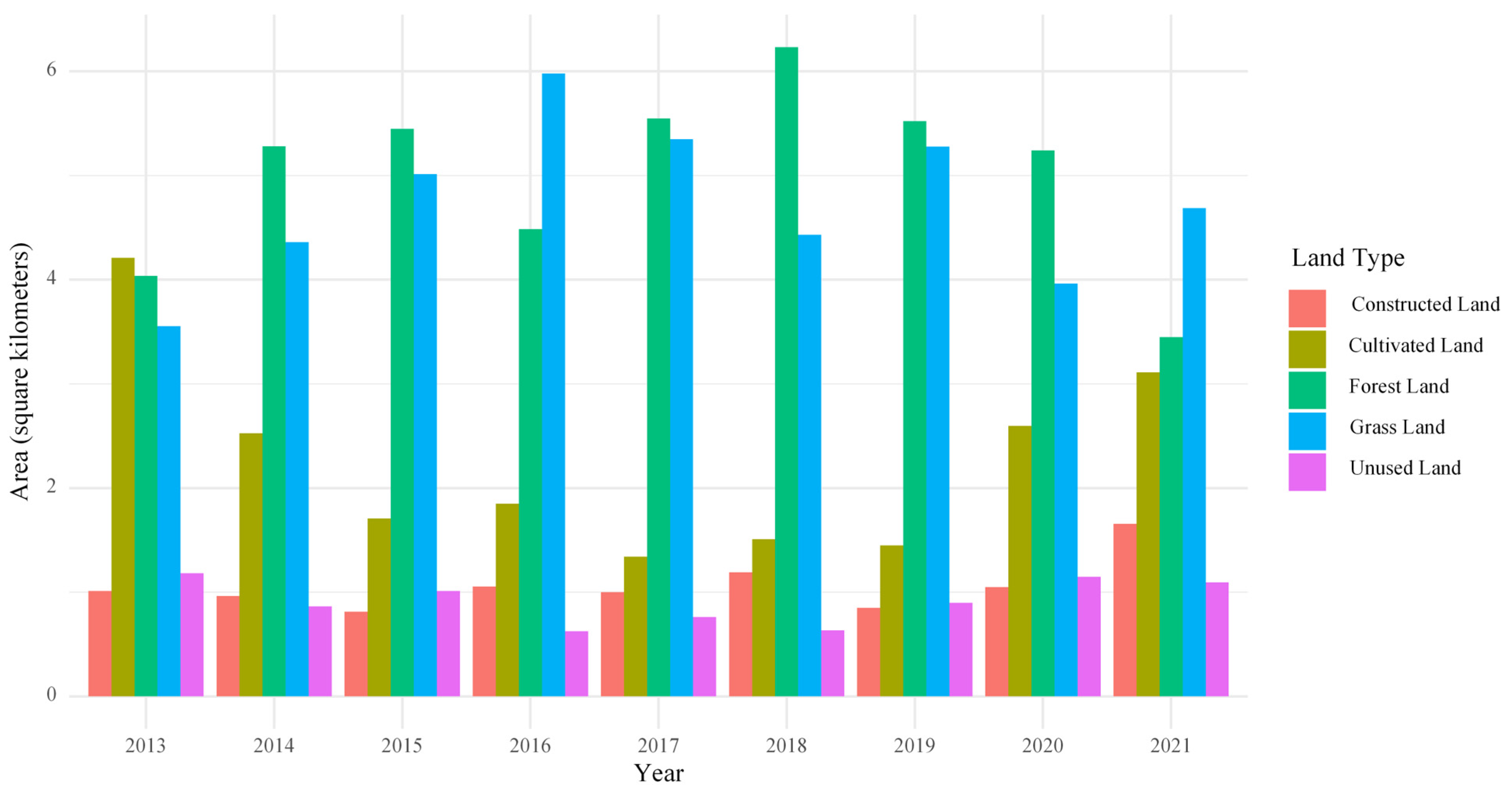
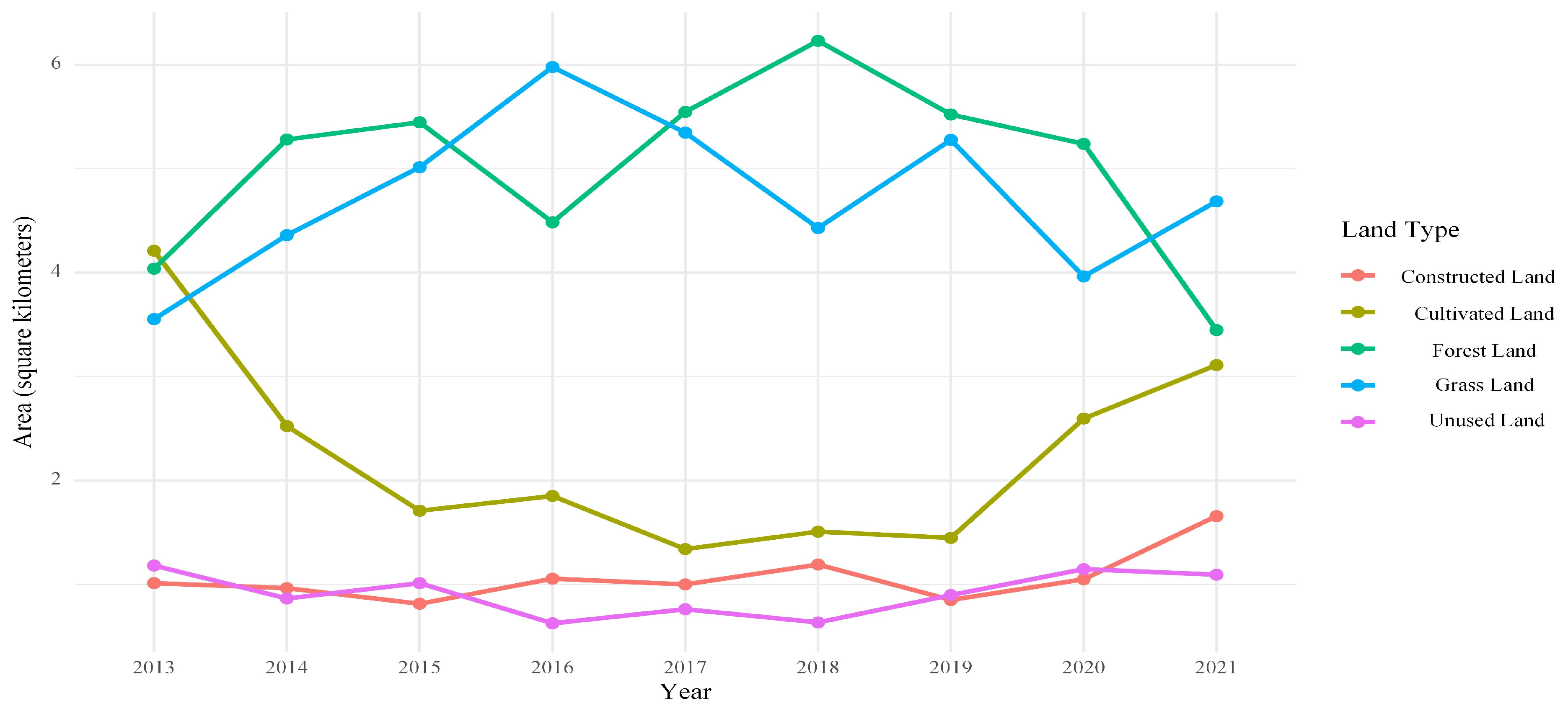
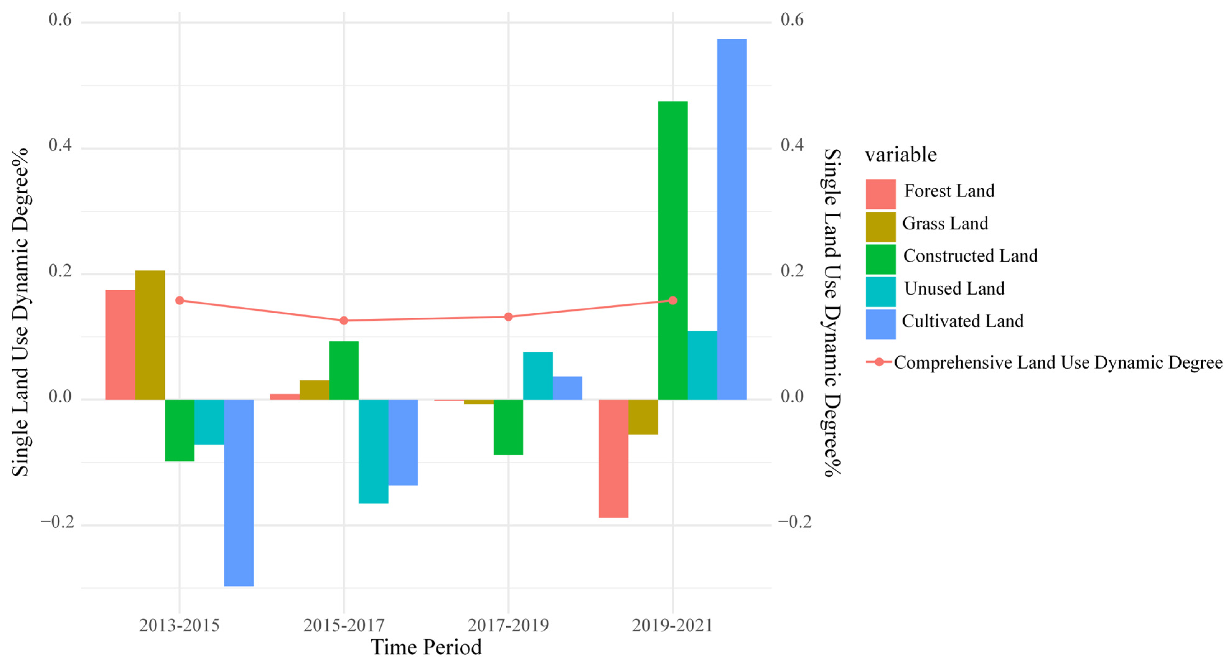
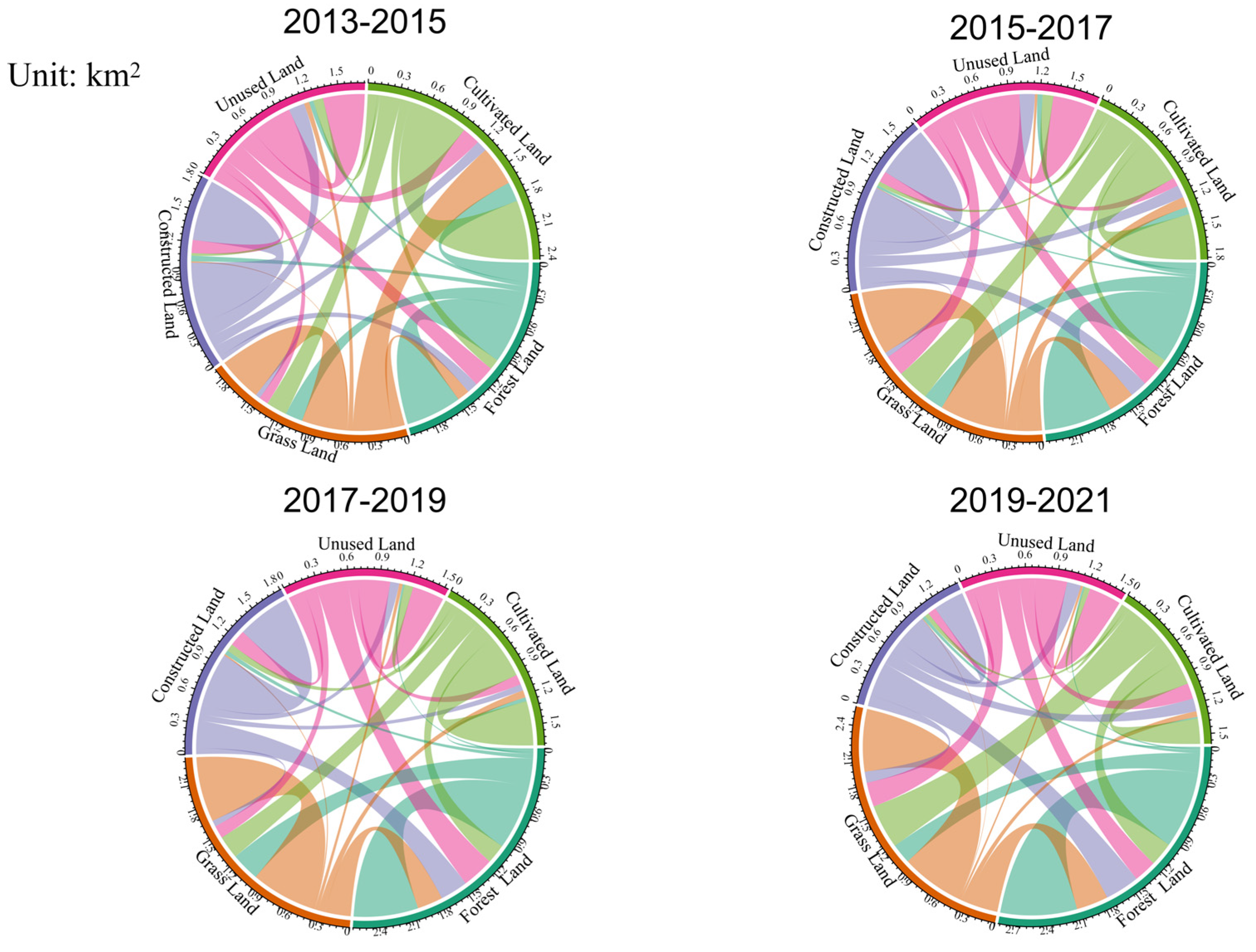
3.1. Land Use Changes in the Overlay Area Between 2013 and 2021

After categorizing the land use in the overlay area, we obtained a map illustrating the spatial changes in each land use classification from 2013 to 2021 (Figure 3). Figure 3 and Figure 4 show that the predominant land use types in the overlay area are forestland and grassland, which collectively occupy 54% of the total area. From 2013 to 2021, the area of forestland initially increased and then decreased. Despite YME being a mining area during this period, the ecological environment of the overlap area still showed an improving trend. Notably, in 2018, the area of forestland reached its peak. In Figure 5, we can observe a substantial reduction in the forestland area from 2019 to 2021. Concurrently, the grassland area showed a fluctuating downward trend during 2019–2021. On the other hand, the constructed land area exhibited a steady increase, which was particularly significant during 2019–2021. The area of unused land dropped to its lowest level in 2016 but has since rebounded. The cultivated land area continued to decrease between 2013 and 2017 but gradually increased from 2019 to 2021.

The dynamics of land use are a crucial indicator of the quantitative changes in land use types over a specific period. This indicator reveals the intensity of land use change and regional differences in the pace of change. Based on the analysis of land use dynamics presented in Figure 6, it is evident that various land types underwent substantial changes between 2013 and 2021. During 2013–2015 and 2015–2017, forestland and grassland showed higher growth rates, indicating an increase in these land types. Although the growth rate for forestland and grassland slowed during 2015–2017, it remained positive, suggesting continued expansion. From 2017 to 2019, the growth rates for these land types turned negative, but the decreases were minimal. However, from 2019 to 2021, the growth rates for forestland and grassland became significantly negative, indicating a marked decrease and an accelerating rate of decline.

In contrast, the growth rate of constructed land surged to 0.48 during 2019–2021, highlighting rapid expansion and increased human activity in the overlay area. The growth rate of unused land fluctuated over time but showed an increase in the final period, suggesting that unused land is being converted to other types, such as constructed or cultivated land. Notably, cultivated land had the highest growth rate during 2019–2021 at 0.57, indicating a substantial increase.

Overall, despite significant changes in individual land types, the integrated land use growth rate suggests that the overall land use change remained relatively balanced.

Between 2013 and 2021, the land use transfer matrix of the overlay area reflects the conversion trends between different land use types. This study focuses on the land use shifts during 2019–2021. During the depicted time period (as shown in Figure 7 and

Table 4. Overlay area’s land use transfer matrix, 2019–2021.

Area (km2)		2021
		Forest Land	Grass Land	Constructed Land	Unused Land	Cultivated Land	Total
2019	Forest Land	0.00	1.83	0.70	0.31	0.91	3.75
	Grass Land	0.84	0.00	0.23	0.33	1.69	3.09
	Constructed Land	0.14	0.04	0.00	0.11	0.16	0.45
	Unused Land	0.08	0.13	0.29	0.00	0.21	0.70
	Cultivated Land	0.06	0.33	0.26	0.21	0.00	0.87
	Total	1.12	2.34	1.48	0.95	2.97	8.86

), forested land underwent significant changes, primarily transforming into grassland and cultivated land. Specifically, approximately 1.83 km² shifted to grassland, while 0.91 km² transitioned to cultivated land. Grassland primarily transformed into cultivated land, with a total conversion area of up to 1.69 km². Unused land was mainly converted into constructed and cultivated land, with conversion areas of 0.29 km² and 0.21 km², respectively. Conversely, cultivated land was largely converted into grassland, resulting in a decrease of 0.87 km².

Overall, forestland and grassland are the land types that experienced the most significant decreases in area, while grassland and cultivated land saw the most significant increases. In 2021, cultivated land experienced the greatest increase in the area, totaling 2.97 km², followed by grassland, with an increase of 2.34 km². These results demonstrate a dynamic conversion relationship between land use types.

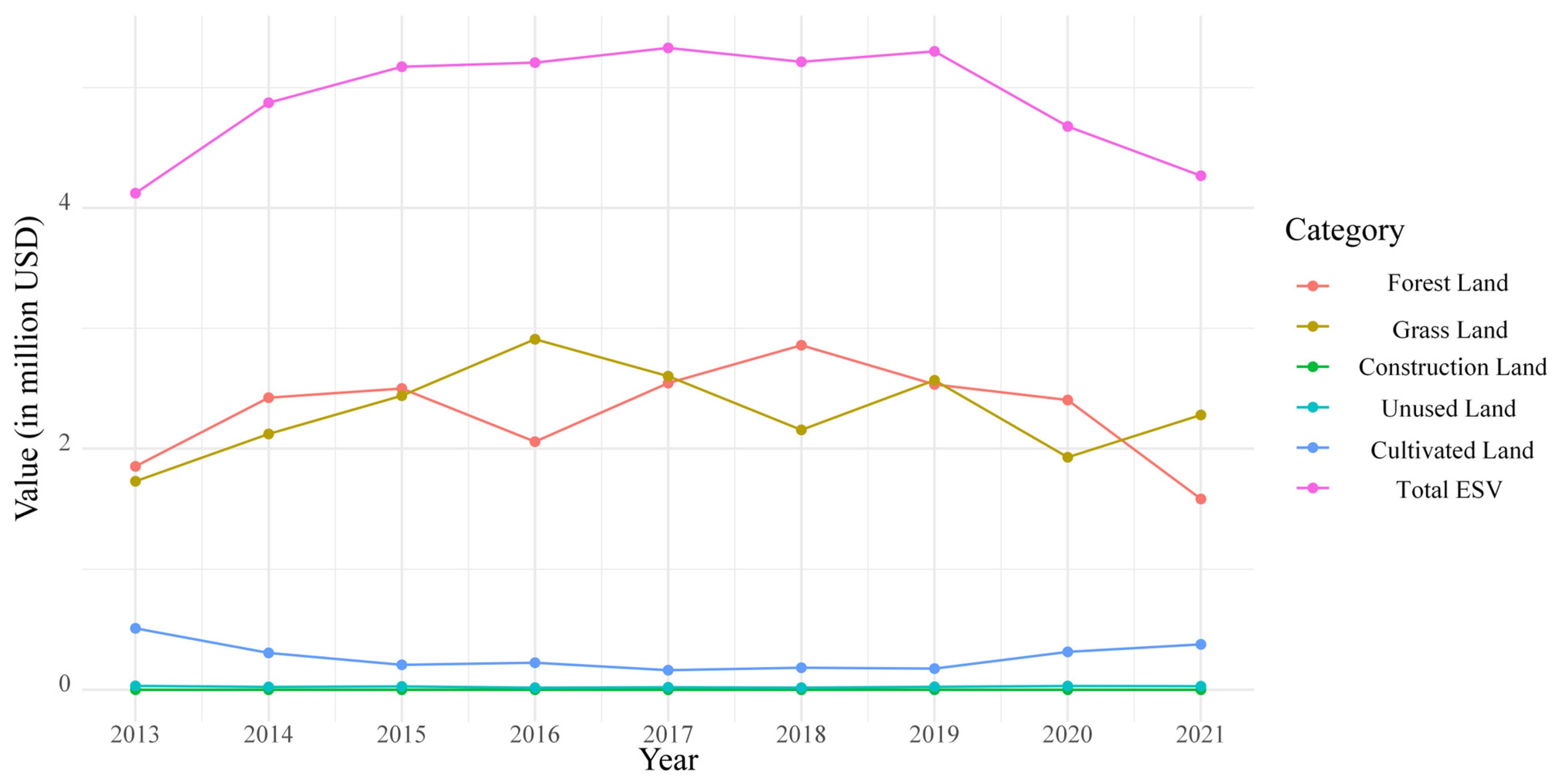
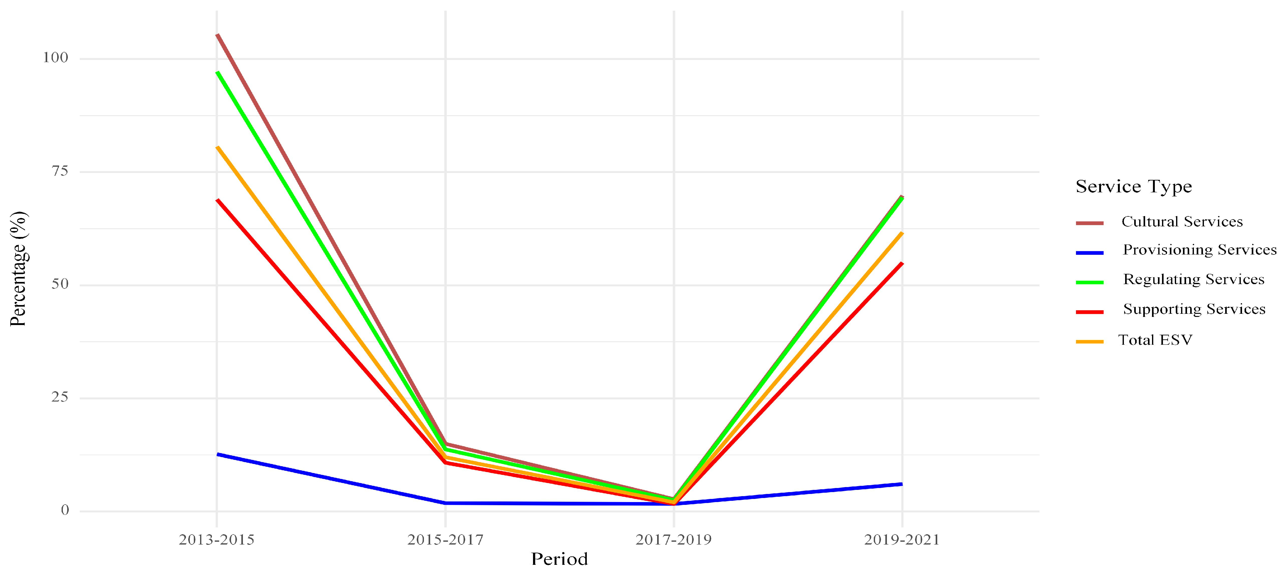
3.2. Changes in ESV Based on Land Use Type Between 2013 and 2021 in the Overlay Area

Between 2013 and 2021, the total ecosystem service value (ESV) of the overlay area underwent significant changes. Figure 8 illustrates that the total ecosystem service value (ESV) increased by 28.60% between 2013 and 2019, followed by a decline in 2020 and 2021. By 2021, the ESV was 19.50% lower than in 2019. The ESVs of both forestland and grassland showed an overall upward trend from 2013 to 2019 but experienced a decline in the subsequent two years. Specifically, forestland’s ESV saw a 37.50% decrease in 2021 compared with 2019. This decline is particularly significant given that forestland and grassland make up the largest percentage of land use in the overlay area, both showing notable decreases in area from 2013 to 2021. The ESV of unused land displayed minor fluctuations throughout the period, with a slight overall increase. In contrast, the ESV of cultivated land decreased by 64.10% between 2013 and 2018 and then reversed to an upward trend from 2019 to 2021, with a 14.8% rise by 2021 compared with 2019. Forestland’s ESV, in particular, exhibited the most rapid change: a 24.70% increase between 2013 and 2018, followed by an 11.20% decrease between 2019 and 2021.

These patterns suggest that various events or factors between 2013 and 2021 influenced these changes. The findings underscore the significant impact of land use changes on ESVs.

3.3. Analysis of Ecological Contribution Rate

The ecological contribution ratio quantifies the extent to which each land use type influences changes in the overall ecosystem service value of a region over a specific period. This metric is crucial for identifying the primary drivers behind fluctuations in regional ESVs. During the period from 2013 to 2021, the rate of change was influenced by the interconversion of land use types. Forestland and grassland in the overlay area exhibited the highest ecological contribution rates, collectively accounting for 85.87% of the total ecological contribution (as shown in

Table 5. Ecological contribution of each land use type, 2013–2021.

Category	Ecological Contribution Ratio
Forestland	28.29%
Grassland	57.58%
Constructed Land	0.00%
Unused Land	0.25%
Cultivated Land	13.89%

). The ecosystem service value equivalence coefficient (ESV) quantifies the socio-economic benefits that are provided by ecological services per unit area for different land use types. Our study found that forests and grasslands made substantial contributions to the overall ESV, meaning that fluctuations in their area significantly affected the total value. While these land types inherently possess high equivalence coefficients that boost their per-unit ecosystem service value, their significant ecological contributions were also driven by significant changes in their areas. In short, the high contribution rates of forests and grasslands reflect both their intrinsic service values and the crucial impact of their area dynamics on the overall ESV.

3.4. Change in Individual ESVs of Overlay Area, 2013–2021

In the study area, mining activities and land use changes had the greatest impact on ecosystem regulation services. These fluctuations directly reflect changes in ecological functioning, making them a focal point of this study. In contrast, provisioning, supporting, and cultural services were less affected by direct human disturbances and natural conditions, or their changes were not significant enough to warrant detailed analysis. Therefore, this study primarily focused on an in-depth investigation of ecosystem regulation services. In the study of ESVs, regulation services refer to the role of ecosystems in managing natural processes such as gas regulation, climate regulation, hydrological regulation, and environmental purification. These services are essential for maintaining environmental stability and human well-being. According to Table 2, which lists ESV equivalents per unit area for each land type in the overlay area, grassland had the highest value for regulation services, followed by forestland. Figure 9, which shows the changes in individual ESVs in the overlay area from 2013 to 2021, reveals that the value of regulation services increased gradually from 2013 to 2018. However, a clear decreasing trend can be observed from 2018 to 2021. This trend was primarily due to increases in the land use areas of forestland and grassland during 2013–2018, followed by significant decreases in these land use areas during 2018–2021.

3.5. Sensitivity Analysis of ESV to Land Use Change

The sensitivity of the ecosystem service value (ESV) to changes in land use dynamics indicates the extent to which land use changes impact the ESV. Between 2013 and 2021, the sensitivity indices of the ESV to changes in land use dynamics for four periods were 80.66%, 12.00%, 2.03%, and 61.70%, respectively. These figures show that for every 1% change in integrated land use dynamics, the ESV changed by 80.66%, 12.00%, 2.03%, and 61.70% during these periods. As shown in Figure 10, the sensitivity index of the ESV to land use changes decreased sharply from 80.66% to a low of 2.03%, before rising significantly to 61.70%. The periods from 2013 to 2015 and 2019 to 2021 exhibited higher sensitivities of the ESV to dynamic land use changes, indicating that land use changes during these time periods had a greater impact on the ESV.

3.6. Analysis of Local Resident Survey Results

Coal mining activities in the YME area are well known and exert a profound influence on both the local economy and the daily lives of nearby communities. As presented in

Table 6. Analysis of the statistical results of the questionnaire survey.

Content	Options	Percentage%
1. Are you aware of the coal mining activities at YME Second Mine?	Yes	64.90
	No	13.90
	Heard of it	20.90
2. Were you involved in the relocation due to previous production activities or nature reserve protection at YME?	Yes	88.40
	No	11.60
3. The reason for your relocation back to the overlapping area of YME Second Mine?	Difficult to integrate into the new community	28.30
	Sense of belonging	24.70
	Regained stable income through farming	47.00
4. Do you farm the land in the overlapping area of YME Second Mine?	Yes	92.60
	No	7.40
5. Do you need to cut down trees to obtain firewood for daily heating and cooking?	Yes	98.80
	No	1.20

, a significant number of residents opted to return to the overlay zone after their relocation. They attributed their decision to several key factors: difficulties adapting to the new community, a deep-seated sense of attachment to their hometowns, and a stable agricultural income. The majority of these residents engaged in farming within the overlay zone, relying on activities such as cutting trees for heating and gathering firewood for cooking. These practices may have negative consequences, such as the transformation of local forestland, cultivated land, and grassland.

3.7. Impact of Land Use Changes on ESV

Land use changes significantly influence the ESV, making the assessment of this value crucial for evaluating land use patterns in mining areas. By examining the evolution of land use in the overlap area and its impact on the ESV, this study identified land use change as the primary driver of ESV fluctuations.

Between 2013 and 2021, the ESV in the overlap area initially increased before declining. Forestland and grassland areas expanded before contracting, while cultivated land decreased initially and later rebounded. Our ecological sensitivity analysis indicated that, from 2017 to 2019, the ESV was the least affected by land use changes, reflecting a period of relative stability. During this period, the Yangquan Forestry Bureau issued directive “Yanglin Bizi [2017] No. 27” (15 May 2017), mandating a comprehensive prohibition of coal mining within the area overlapping with the nature reserve.

Until 2018, improvements in land cover—particularly the expansion of forestlands and grasslands—led to a significant increase in the ESV, contributing an estimated USD 9.71 billion. Our ecological contribution analysis identified this expansion as the primary driver of the increase. However, from 2018 to 2021, the ESV declined sharply, as forestland and grassland were converted to cultivated land.

These findings underscore the strong link between land use changes and ESV fluctuations, highlighting the high sensitivity of the ESV to land use dynamics. The 2018 coal mining ban marked a key turning point, demonstrating the impact of policy interventions on ESV trends.

3.8. Implications of ESV for Ecological Impacts of Coal Mining on Overlapping Areas at YME

The mining area, characterized by intense human activity and rapid land use changes, contrasts with the natural ecological reserve, where human influence is minimal. When these two areas overlap, how do land use and land cover changes affect the ecosystem service value (ESV)? As land use changes play a key role in defining the ESV, and the ecosystem’s health underpins ecosystem services [68,69], this study examined these dynamics through field visits and interviews with local villagers.

Between 2013 and 2018, coal mining operations in the overlap area led to the relocation and resettlement of local villagers, leaving large tracts of cultivated land abandoned. With reduced human activity, the vegetation in forests and grasslands regenerated, increasing the forest coverage by 2.19 km². However, in 2018, the Pingding County government issued a ban on mining to protect the Guanshan Mountain Provincial Nature Reserve, ending the monetary compensation for displaced villagers. As a result, many returned, reclaiming land for cultivation, cutting trees for fuel, and rebuilding homes. Between 2018 and 2021, these activities led to a sharp decline in forest and grassland coverage, while cultivated land and built-up areas expanded.

Contrary to widespread findings that coal mining severely degrades ecosystems, this study observed an initial environmental improvement due to reduced human activity during mining operations, followed by ecological decline after mining ceased and human activity rebounded. Possible explanations include the significant shifts in human land use behavior that occurred before and after these mining activities [70], along with the inherent natural resilience, which is evident within the boundaries of the protected reserve [71]. However, this study had certain methodological and data limitations. Future research should assess the broader environmental effects of coal mining over a larger spatial scale and longer time frame.

4. Conclusions and Recommendations

In this study, the following conclusions were drawn from our in-depth analysis of land use changes and their impact on the ecosystem service value (ESV) in the overlap area between Yang Coal Mine No. 2 and Shanxi Yakulinji Guanshan Provincial Nature Reserve:

(1)

Trend of land use change: Between 2013 and 2021, significant changes in land use types were observed in the overlap area. From 2013 to 2018, the areas of forestland and grassland increased, while from 2018 to 2021, these areas decreased, primarily being converted into cultivated land. These shifts were mainly driven by human activities.

(2)

Impact of land use change on ESV: Land use changes in the overlap area were found to be the primary driver of fluctuations in the ecosystem service value (ESV).

(3)

Impacts of coal mining on ESV: Coal mining activities did not result in significant ecological damage in the overlap area. However, between 2018 and 2021, a noticeable decline in the ESV occurred as human activities increased, particularly with the expansion of cultivated land. The cessation of coal mining, combined with changes in human activities, was the primary factor influencing ESV fluctuations.

This study highlights the significant influence of land use changes and human activities on the ecosystem service value, providing essential insights for understanding and managing ESVs in mining areas. Based on these findings, the following recommendations are proposed to enhance ecosystem protection in the overlap area:

(1)

Rational land use planning: Land use decisions should account for their impact on the ecosystem service value (ESV). Efforts to maintain ecosystem stability should focus on increasing the proportion of forest and grassland areas.

(2)

Ecological restoration and protection: Following the cessation of mining activities, efforts should be made to restore forest and grassland areas, particularly by planting local endemic species to strengthen the ecosystem’s resilience. Additionally, nature reserve protections should be reinforced to prevent illegal logging and overgrazing.

(3)

Alternative livelihoods for local communities: As mining ceases and people return to the overlap area, agricultural expansion may occur. To mitigate the pressure on the land, alternative livelihood opportunities—such as ecotourism and job training programs—should be introduced to reduce the dependence on arable land.

References

1. Zhironkin, S.; Cehlár, M. Coal Mining Sustainable Development: Economics and Technological Outlook. Energies 2021, 14, 5029. [Google Scholar] [CrossRef]
2. Ma, K.; Zhang, Y.; Ruan, M.; Guo, J.; Chai, T. Land Subsidence in a Coal Mining Area Reduced Soil Fertility and Led to Soil Degradation in Arid and Semi-Arid Regions. Int. J. Environ. Res. Public Health 2019, 16, 3929. [Google Scholar] [CrossRef]
3. Guo, W.; Guo, M.; Tan, Y.; Bai, E.; Zhao, G. Sustainable Development of Resources and the Environment: Mining-Induced Eco-Geological Environmental Damage and Mitigation Measures—A Case Study in the Henan Coal Mining Area, China. Sustainability 2019, 11, 4366. [Google Scholar] [CrossRef]
4. Ogola, J.S.; Mitullah, W.V.; Omulo, M.A. Impact of gold mining on the environment and human health: A case study in the Migori gold belt, Kenya. Environ. Geochem. Health 2002, 24, 141–157. [Google Scholar] [CrossRef]
5. Barnett, J.; Matthew, R.A.; O’Brien, K.L. Global environmental change and human security: An introduction. In Global Environmental Change and Human Security; MIT Press: Cambridge, MA, USA, 2009; pp. 3–32. [Google Scholar]
6. Du, L.; Hou, Y.; Zhong, S.; Qu, K. Identification of Priority Areas for Ecological Restoration in Coal Mining Areas with a High Groundwater Table Based on Ecological Security Pattern and Ecological Vulnerability. Sustainability 2024, 16, 159. [Google Scholar]
7. Polasky, S.; Nelson, E.; Pennington, D.; Johnson, K.A. The impact of land-use change on ecosystem services, biodiversity and returns to landowners: A case study in the state of Minnesota. Environ. Resour. Econ. 2011, 48, 219–242. [Google Scholar]
8. Deng, X.; Li, Z.; Gibson, J. A review on trade-off analysis of ecosystem services for sustainable land-use management. J. Geogr. Sci. 2016, 26, 953–968. [Google Scholar] [CrossRef]
9. Tariq, A.; Graciano, C.; Sardans, J.; Zeng, F.; Hughes, A.C.; Ahmed, Z.; Ullah, A.; Ali, S.; Gao, Y.; Peñuelas, J. Plant root mechanisms and their effects on carbon and nutrient accumulation in desert ecosystems under changes in land use and climate. New Phytol. 2024, 242, 916–934. [Google Scholar]
10. Esty, D.C. Greening the GATT: Trade, environment, and the future: Peterson Institute. Fuel Energy Abstr. 1994, 5, 371. [Google Scholar]
11. Haines-Young, R.; Potschin, M. The links between biodiversity, ecosystem services and human well-being. Ecosyst. Ecol. A New Synth. 2010, 1, 110–139. [Google Scholar]
12. Kneeshaw, D.D.; Leduc, A.; Messier, C.; Drapeau, P.; Gauthier, S.; Paré, D.; Carignan, R.; Doucet, R.; Bouthillier, L. Development of integrated ecological standards of sustainable forest management at an operational scale. For. Chron. 2000, 76, 481–493. [Google Scholar]
13. Bengtsson, J.; Angelstam, P.; Elmqvist, T.; Emanuelsson, U.; Folke, C.; Ihse, M.; Moberg, F.; Nyström, M. Reserves, resilience and dynamic landscapes. AMBIO J. Hum. Environ. 2003, 32, 389–396. [Google Scholar]
14. Costanza, R.; D’Arge, R.; De Groot, R.; Farber, S.; Grasso, M.; Hannon, B.; Limburg, K.; Naeem, S.; O’Neill, R.V.; Paruelo, J. The value of the world’s ecosystem services and natural capital. Nature 1997, 387, 253–260. [Google Scholar]
15. Xie, G.; Zhen, L.; LU, C.; Xiao, Y.; Chen, C. Expert knowledge based valuation method of ecosystem services in China. J. Nat. Resour. 2008, 23, 911–919. [Google Scholar]
16. Xie, G.; Xiao, Y. Review of agro-ecosystem services and their values. Chin. J. Eco-Agric. 2013, 21, 645–651. [Google Scholar]
17. Xie, G.D.; Xiao, Y.; LU, C.X. Study on ecosystem services: Progress, limitation and basic paradigm. Chin. J. Plant Ecol. 2006, 30, 191. [Google Scholar]
18. Xie, G.; Zhang, C.; Zhang, C.; Xiao, Y.; Lu, C. The value of ecosystem services in China. Resour. Sci. 2015, 37, 1740–1746. [Google Scholar]
19. Qian, D.; Yan, C.; Xiu, L.; Feng, K. The impact of mining changes on surrounding lands and ecosystem service value in the Southern Slope of Qilian Mountains. Ecol. Complex. 2018, 36, 138–148. [Google Scholar]
20. Quan, L.A.; Jin, S.; Chen, J.; Li, T. Evolution and Driving Forces of Ecological Service Value in Anhui Based on Landsat Land Use and Land Cover Change. Remote Sens. 2024, 16, 269. [Google Scholar] [CrossRef]
21. Zhang, B.; Feng, Q.; Li, Z.; Lu, Z.; Zhang, B.; Cheng, W. Land Use/Cover-Related Ecosystem Service Value in Fragile Ecological Environments: A Case Study in Hexi Region, China. Remote Sens. 2024, 16, 563. [Google Scholar] [CrossRef]
22. Qian, D.; Yang, C.; Xiu, L. Land cover change and landscape pattern vulnerability response in Muli mining and its surrounding areas in the Qinghai-Tibet Plateau. J. Glaciol. Geocryol. 2020, 42, 1334–1343. [Google Scholar]
23. Geist, H.; McConnell, W.; Lambin, E.F.; Moran, E.; Alves, D.; Rudel, T. Causes and trajectories of land-use/cover change. In Land-Use and Land-Cover Change: Local Processes and Global Impacts; Springer: Berlin/Heidelberg, Germany, 2006; pp. 41–70. [Google Scholar]
24. Maxwell, A.E.; Warner, T.A.; Fang, F. Implementation of machine-learning classification in remote sensing: An applied review. Int. J. Remote Sens. 2018, 39, 2784–2817. [Google Scholar] [CrossRef]
25. Tolessa, T.; Senbeta, F.; Kidane, M. The impact of land use/land cover change on ecosystem services in the central highlands of Ethiopia. Ecosyst. Serv. 2017, 23, 47–54. [Google Scholar] [CrossRef]
26. Feng, H.; Zhang, X.; Nan, Y.; Zhang, D.; Sun, Y. Ecological Sensitivity Assessment and Spatial Pattern Analysis of Land Resources in Tumen River Basin, China. Appl. Sci. 2023, 13, 4197. [Google Scholar] [CrossRef]
27. Hu, X.; Ma, C.; Huang, P.; Guo, X. Ecological vulnerability assessment based on AHP-PSR method and analysis of its single parameter sensitivity and spatial autocorrelation for ecological protection—A case of Weifang City, China. Ecol. Indic. 2021, 125, 107464. [Google Scholar] [CrossRef]
28. Querol, X.; Izquierdo, M.; Monfort, E.; Álvarez, E.; Font, O.; Moreno, T.; Alastuey, A.; Zhuang, X.; Lu, W.; Wang, Y. Environmental characterization of burnt coal gangue banks at Yangquan, Shanxi Province, China. Int. J. Coal Geol. 2008, 75, 93–104. [Google Scholar] [CrossRef]
29. Zheng, Q.; Shi, S.; Liu, Q.; Xu, Z. Modes of occurrences of major and trace elements in coals from Yangquan Mining District, North China. J. Geochem. Explor. 2017, 175, 36–47. [Google Scholar] [CrossRef]
30. Shelestov, A.; Lavreniuk, M.; Kussul, N.; Novikov, A.; Skakun, S. Exploring Google Earth Engine platform for big data processing: Classification of multi-temporal satellite imagery for crop mapping. Front. Earth Sci. 2017, 5, 232994. [Google Scholar] [CrossRef]
31. Amani, M.; Ghorbanian, A.; Ahmadi, S.A.; Kakooei, M.; Moghimi, A.; Mirmazloumi, S.M.; Moghaddam, S.H.A.; Mahdavi, S.; Ghahremanloo, M.; Parsian, S. Google earth engine cloud computing platform for remote sensing big data applications: A comprehensive review. IEEE J. Sel. Top. Appl. Earth Observ. Remote Sens. 2020, 13, 5326–5350. [Google Scholar] [CrossRef]
32. Elmahal, A.; Ganwa, E. Advanced Digital Image Analysis of Remotely Sensed Data Using JavaScript API and Google Earth Engine. In Revolutionizing Earth Observation—New Technologies and Insights; Intechopen: London, UK, 2024. [Google Scholar]
33. Ye, J.; Hu, Y.; Zhen, L.; Wang, H.; Zhang, Y. Analysis on Land-Use Change and its driving mechanism in Xilingol, China, during 2000–2020 using the google earth engine. Remote Sens. 2021, 13, 5134. [Google Scholar] [CrossRef]
34. Topaloğlu, R.H.; Sertel, E.; Musaoğlu, N. Assessment of classification accuracies of Sentinel-2 and Landsat-8 data for land cover/use mapping. Int. Arch. Photogramm. Remote Sens. Spat. Inf. Sci. 2016, 41, 1055–1059. [Google Scholar] [CrossRef]
35. Radoux, J.; Chomé, G.; Jacques, D.C.; Waldner, F.; Bellemans, N.; Matton, N.; Lamarche, C.; D Andrimont, R.; Defourny, P. Sentinel-2’s potential for sub-pixel landscape feature detection. Remote Sens. 2016, 8, 488. [Google Scholar] [CrossRef]
36. Chen, J.; Chen, J.; Liao, A.; Cao, X.; Chen, L.; Chen, X.; He, C.; Han, G.; Peng, S.; Lu, M. Global land cover mapping at 30 m resolution: A POK-based operational approach. ISPRS-J. Photogramm. Remote Sens. 2015, 103, 7–27. [Google Scholar]
37. Roy, D.P.; Wulder, M.A.; Loveland, T.R.; Woodcock, C.E.; Allen, R.G.; Anderson, M.C.; Helder, D.; Irons, J.R.; Johnson, D.M.; Kennedy, R. Landsat-8: Science and product vision for terrestrial global change research. Remote Sens. Environ. 2014, 145, 154–172. [Google Scholar] [CrossRef]
38. Xu, C.; Liu, H.; Williams, A.P.; Yin, Y.; Wu, X. Trends toward an earlier peak of the growing season in Northern Hemisphere mid-latitudes. Glob. Change Biol. 2016, 22, 2852–2860. [Google Scholar] [CrossRef]
39. Guan, X.; Guo, S.; Huang, J.; Shen, X.; Fu, L.; Zhang, G. Effect of seasonal snow on the start of growing season of typical vegetation in Northern Hemisphere. Geogr. Sustain. 2022, 3, 268–276. [Google Scholar]
40. Jeong, S.J.; HO, C.H.; GIM, H.J.; Brown, M.E. Phenology shifts at start vs. end of growing season in temperate vegetation over the Northern Hemisphere for the period 1982–2008. Glob. Change Biol. 2011, 17, 2385–2399. [Google Scholar]
41. Tasser, E.; Walde, J.; Tappeiner, U.; Teutsch, A.; Noggler, W. Land-use changes and natural reforestation in the Eastern Central Alps. Agric. Ecosyst. Environ. 2007, 118, 115–129. [Google Scholar]
42. Rouse, J.W., Jr.; Haas, R.H.; Deering, D.W.; Schell, J.A.; Harlan, J.C. Monitoring the Vernal Advancement and Retrogradation (Green Wave Effect) of Natural Vegetation. 1974. Available online: https://ntrs.nasa.gov/citations/19740022555 (accessed on 1 July 2024).
43. Soudani, K.; Hmimina, G.; Delpierre, N.; Pontailler, J.; Aubinet, M.; Bonal, D.; Caquet, B.; De Grandcourt, A.; Burban, B.; Flechard, C. Ground-based Network of NDVI measurements for tracking temporal dynamics of canopy structure and vegetation phenology in different biomes. Remote Sens. Environ. 2012, 123, 234–245. [Google Scholar]
44. Zhang, Y.; Odeh, I.O.; Ramadan, E. Assessment of land surface temperature in relation to landscape metrics and fractional vegetation cover in an urban/peri-urban region using Landsat data. Int. J. Remote Sens. 2013, 34, 168–189. [Google Scholar]
45. Pettorelli, N. Satellite Remote Sensing and the Management of Natural Resources; Oxford University Press: Oxford, UK, 2019. [Google Scholar]
46. Rock, B.N.; Skole, D.L.; Choudhury, B.J. Monitoring vegetation change using satellite data. In Vegetation Dynamics & Global Change; Springer: Berlin/Heidelberg, Germany, 1993; pp. 153–167. [Google Scholar]
47. Townshend, J.R.; Justice, C.O. Selecting the spatial resolution of satellite sensors required for global monitoring of land transformations. Int. J. Remote Sens. 1988, 9, 187–236. [Google Scholar]
48. Huang, S.; Tang, L.; Hupy, J.P.; Wang, Y.; Shao, G. A commentary review on the use of normalized difference vegetation index (NDVI) in the era of popular remote sensing. J. For. Res. 2021, 32, 1–6. [Google Scholar]
49. Eastman, J.R.; Sangermano, F.; Machado, E.A.; Rogan, J.; Anyamba, A. Global trends in seasonality of normalized difference vegetation index (NDVI). Remote Sens. 2013, 5, 4799–4818. [Google Scholar] [CrossRef]
50. Pettorelli, N.; Ryan, S.; Mueller, T.; Bunnefeld, N.; Jędrzejewska, B.; Lima, M.; Kausrud, K. The Normalized Difference Vegetation Index (NDVI): Unforeseen successes in animal ecology. Clim. Res. 2011, 46, 15–27. [Google Scholar]
51. Wiethase, J.H. Advancing Ecosystem Understanding: Identifying the Drivers of Habitat Degradation, Species Distributions and Species Vulnerabilities in East African Grasslands. Ph.D. Thesis, University of York, York, UK, 2023. [Google Scholar]
52. Hayes, M.M.; Miller, S.N.; Murphy, M.A. High-resolution landcover classification using Random Forest. Remote Sens. Lett. 2014, 5, 112–121. [Google Scholar]
53. GB/T 21010-2017; Current Land Use Classification. China Standards Press: Beijing, China, 2017.
54. Yin, L.; Chen, K.; Jiang, Z.; Xu, X. A fast parallel random forest algorithm based on spark. Appl. Sci. 2023, 13, 6121. [Google Scholar]
55. Joelsson, S.R.; Benediktsson, J.A.; Sveinsson, J.R. Random forest classification of remote sensing data. In Signal and Image Processing for Remote Sensing; CRC Press: Boca Raton, FL, USA, 2006; pp. 344–361. [Google Scholar]
56. Ayala-Izurieta, J.E.; Márquez, C.O.; García, V.J.; Recalde-Moreno, C.G.; Rodríguez-Llerena, M.V.; Damián-Carrión, D.A. Land cover classification in an ecuadorian mountain geosystem using a random forest classifier, spectral vegetation indices, and ancillary geographic data. Geosciences 2017, 7, 34. [Google Scholar] [CrossRef]
57. Foody, G.M. Explaining the unsuitability of the kappa coefficient in the assessment and comparison of the accuracy of thematic maps obtained by image classification. Remote Sens. Environ. 2020, 239, 111630. [Google Scholar]
58. Fonseca, J.; Douzas, G.; Bacao, F. Improving imbalanced land cover classification with K-Means SMOTE: Detecting and oversampling distinctive minority spectral signatures. Information 2021, 12, 266. [Google Scholar] [CrossRef]
59. Barthakur, A.; Joksimovic, S.; Kovanovic, V.; Mello, R.F.; Taylor, M.; Richey, M.; Pardo, A. Understanding depth of reflective writing in workplace learning assessments using machine learning classification. IEEE Trans. Learn. Technol. 2022, 15, 567–578. [Google Scholar]
60. Liping, C.; Yujun, S.; Saeed, S. Monitoring and predicting land use and land cover changes using remote sensing and GIS techniques—A case study of a hilly area, Jiangle, China. PLoS ONE 2018, 13, e0200493. [Google Scholar] [CrossRef] [PubMed]
61. Cihlar, J.; Jansen, L.J. From land cover to land use: A methodology for efficient land use mapping over large areas. Prof. Geogr. 2001, 53, 275–289. [Google Scholar] [CrossRef]
62. Wang, Z.; Cao, J.; Zhu, C.; Yang, H. The impact of land use change on ecosystem service value in the upstream of Xiong’an new area. Sustainability 2020, 12, 5707. [Google Scholar] [CrossRef]
63. Xie, G.; Zhang, C.; Zhen, L.; Zhang, L. Dynamic changes in the value of China’s ecosystem services. Ecosyst. Serv. 2017, 26, 146–154. [Google Scholar] [CrossRef]
64. Wang, P.; Li, R.; Liu, D.; Wu, Y. Dynamic characteristics and responses of ecosystem services under land use/land cover change scenarios in the Huangshui River Basin, China. Ecol. Indic. 2022, 144, 109539. [Google Scholar]
65. Han, Z.; Song, W.; Deng, X. Responses of ecosystem service to land use change in Qinghai Province. Energies 2016, 9, 303. [Google Scholar] [CrossRef]
66. Arowolo, A.O.; Deng, X.; Olatunji, O.A.; Obayelu, A.E. Assessing changes in the value of ecosystem services in response to land-use/land-cover dynamics in Nigeria. Sci. Total Environ. 2018, 636, 597–609. [Google Scholar]
67. Fowler, F.J., Jr. Survey Research Methods; Sage Publications: Thousand Oaks, CA, USA, 2013. [Google Scholar]
68. Hernández Blanco, M.; Costanza, R.; Chen, H.; DeGroot, D.; Jarvis, D.; Kubiszewski, I.; Montoya, J.; Sangha, K.; Stoeckl, N.; Turner, K. Ecosystem health, ecosystem services, and the well-being of humans and the rest of nature. Glob. Change Biol. 2022, 28, 5027–5040. [Google Scholar]
69. Pan, Z.; He, J.; Liu, D.; Wang, J.; Guo, X. Ecosystem health assessment based on ecological integrity and ecosystem services demand in the Middle Reaches of the Yangtze River Economic Belt, China. Sci. Total Environ. 2021, 774, 144837. [Google Scholar]
70. Sarmiento, R.; Cruz, R.V.; Tiburan, C.; Sobremisana, M.; Bantayan, N. Land Use and Cover Change in Watersheds within Mining Tenements in Agusan Del Norte, Philippines. BIO Web Conf. 2024, 131, 4001. [Google Scholar]
71. Parera, E.; Purwanto, R.H.; Permadi, D.B.; Sumardi, S. Social Ecological Resilience System of Ambon Island Protected Forest, Maluku Province, Indonesia. J. Penelit. Kehutan. Wallacea 2024, 13, 13–24. [Google Scholar] [CrossRef]
Figure 1. Map of the study area.
Remotesensing 17 01139 g001
Figure 2. Research technology roadmaps.
Remotesensing 17 01139 g002
Figure 3. Spatial changes in each land use type in the overlay area, 2013–2021.
Remotesensing 17 01139 g003
Figure 4. Area of each land type per year in the overlay area, 2013–2021.
Remotesensing 17 01139 g004
Figure 5. Changes in area by land type in the overlay area, 2013–2021.
Remotesensing 17 01139 g005
Figure 6. Changes in dynamics of land use by period in the overlap area.
Remotesensing 17 01139 g006
Figure 7. Land transfer changes in the overlay area over four different time periods, 2013–2021.
Remotesensing 17 01139 g007
Figure 8. Changes in ESV by land type in the overlay area between 2013 and 2021.
Remotesensing 17 01139 g008
Figure 9. Change in individual ESVs of overlay area, 2013–2021.
Remotesensing 17 01139 g009
Figure 10. Trends in ecological sensitivity index over time for different time periods.
Remotesensing 17 01139 g010