Contribution of PPP with Ambiguity Resolution to the Maintenance of Terrestrial Reference Frame

Abstract

Precise Point Positioning (PPP) provides static positioning at the millimeter level and kinematic positioning ranging from millimeters to decimeters globally. Unlike the traditional network solution, PPP does not require data from other reference stations. This flexibility enhances the convenience of densifying the reference frame while maintaining the accuracy of solutions. In this study, Precise Point Positioning with Ambiguity Resolution (PPP-AR) was employed instead of a network solution, utilizing the combined orbit, clock, and bias products from IGS Repro3 to resolve the long-term station coordinates and derive their velocities, thereby contributing to the maintenance and densification of the terrestrial reference frame. We selected 46 globally distributed stations and performed PPP-AR over a 5-year period, from 2015.0 to 2020.0. The results show that differences in station coordinates between PPP-AR and IGS Repro3 are almost within 2 mm in the horizontal direction and within 5 mm in the vertical direction after Helmert transformation, which is roughly equivalent to the formal error of IGS solutions. The velocity uncertainty of PPP-AR solutions and the difference between PPP-AR and IGS Repro3 are nearly equal to the formal error of the ITRF horizontal velocity field and slightly exceed that of the IGS horizontal velocity field. The seasonal amplitudes of the remaining stations demonstrate strong consistency. Compared to PPP solutions, PPP-AR solutions provide improved coordinate and velocity precision, particularly in the east component. The consistency between the IGS Repro3 orbit/clock combination and IGS Repro3 position solutions is relatively high. These findings indicate that the PPP-AR technique can derive high-precision station coordinates with a similar level of accuracy to network solutions for supporting the maintenance and densification of the terrestrial reference frame.

1. Introduction

The terrestrial reference frame offers a standardized coordinate system for global measurements, facilitating the monitoring of Earth’s deformation and tectonic activity, and supporting both scientific research and engineering applications. Global Navigation Satellite System (GNSS) technology is essential in establishing the terrestrial reference frame, offering submillimeter-per-year precision. The accuracy of GNSS solutions is generally superior to that of geological data, rendering them indispensable for monitoring tectonic activity and geodynamic processes [1,2]. Currently, GNSS-derived station coordinates can be obtained through two main methods: network solutions and Precise Point Positioning (PPP). The primary input data for the newest International Terrestrial Reference Frame (ITRF2020) is the IGS Repro3 coordinate solution, which is obtained by combining reprocessed solutions from ten Analysis Centers (ACs) [3,4]. The coordinates of most ACs are obtained through network solutions. However, challenges in network solutions, such as the decreased data processing efficiency caused by an increasing number of stations, remain unresolved. When software like GAMIT/GLOBK or Bernese processes over 100 stations simultaneously, it often encounters issues such as large normal equations, memory overflow, and slow computation, rendering whole-network solutions for large-scale GNSS networks impractical [5]. Additionally, adding new stations to densify the reference frame is a complex and challenging task for network solutions.

The single-station PPP method, first introduced by Zumberge et al. in 1997, represented a significant leap forward in global positioning technology [6]. By utilizing precise satellite orbits and clocks, PPP enables accurate positioning of individual stations while accounting for phase ambiguities, zenith tropospheric delays, and receiver clock errors. This method not only enhances operational efficiency but also reduces workload, making it widely applicable in monitoring hazardous events and other critical applications [7]. Over the past two decades, extensive research has been conducted to enhance the accuracy of PPP through the correction of various error sources [8,9,10]. Additionally, the station coordinates derived by PPP are directly aligned to the reference frame used in the precise orbit and clock products, ensuring high consistency and reliability.

Compared to traditional PPP with float solutions, PPP-AR significantly shortens convergence times and enhances positioning precision by resolving integer ambiguities [11,12]. Given these advantages, PPP-AR is a promising technique in maintaining the reference frame and is anticipated to be vital in densifying the reference frame.

Recent studies have applied PPP to analyze coordinate time series and derive velocity fields. Rabah et al. processed 14 days of GNSS data using PPP to obtain precise coordinates of Kuwait’s network, thereby verifying the feasibility of establishing a continuously operating reference station network [13]. García-Armenteros used PPP and double-differencing to generate a 3D velocity field for the Iberia and Nubia plates [2]. Arias-Gallegos et al. employed the GipsyX software in PPP mode to estimate the absolute and residual velocities in Ecuador [14]. Ogutcu et al. utilized PRIDE to monitor the 24 h displacement derived from static and kinematic PPP-AR [15]. Nguyen performed PPP with two different products of IGS and CNES to study tectonic motions in Vietnam between 2019 and 2021 [16]. Chen et al. provided a detailed comparison and analysis of the differences between global and regional station PPP-AR solutions and network solutions [17]. One of the ten IGS ACs, JPL, has recently begun using GPS PPP-AR to estimate station positions [18]. However, the globally distributed station coordinates obtained through muti-GNSS PPP-AR to obtain the global velocity field are not yet widely adopted. Therefore, this study aims to fill this gap by analyzing the accuracy of long-term global station coordinates and velocity fields estimated from PPP-AR solutions, and by providing a foundation for maintaining and densifying the terrestrial reference frame through PPP-AR as a supplementary solution to network solutions.

IGS launched its third reprocessing campaign (Repro3) in response to the ITRF2020 call for participation. By the end of 2021, a total of 10 IGS ACs had released GNSS reprocessing products, including Earth rotation parameters, precise satellite orbits and clock offsets, and pseudorange and phase bias products. The Wuhan University Multi-GNSS experiment (WUM) AC completed the combination of IGS Repro3 clock and bias products for the period 2000–2020 and released its combined products, which are available for download from the IGS Data Center and the Wuhan University IGS Data Center [19]. These precise products play a crucial role in supporting PPP-AR. Therefore, it is essential to assess the positioning accuracy of the Repro3 orbit, clock, and bias products and to verify the consistency between new IGS Repro3 orbit/clock combinations and IGS Repro3 position combinations using PPP-AR.

In this research, we conduct PPP-AR with IGS Repro3 orbit/clock/bias solutions on the observation data spanning from 2015.0 to 2020.0. Considering that the realization of the reference frame is based on the coordinates of the reference stations at the reference epoch, along with their velocities (including linear velocity, seasonal term amplitude, and phase), we analyze the precision of PPP-AR coordinate solutions, as well as the fitted velocity field and seasonal terms. The structure of the paper is as follows: Section 2 outlines the data and methodology, detailing the selection of 46 IGS stations from 2015.0 to 2020.0 and the application of PPP-AR using Net_Diff software (Version 1.17) [20]. Section 3 presents the results, including accuracy analysis of station coordinates, velocity fields, and seasonal term estimates. Additionally, results from PPP without Ambiguity Resolution are also discussed in Section 4. Finally, Section 5 presents the conclusions.

2. Data and Methodology

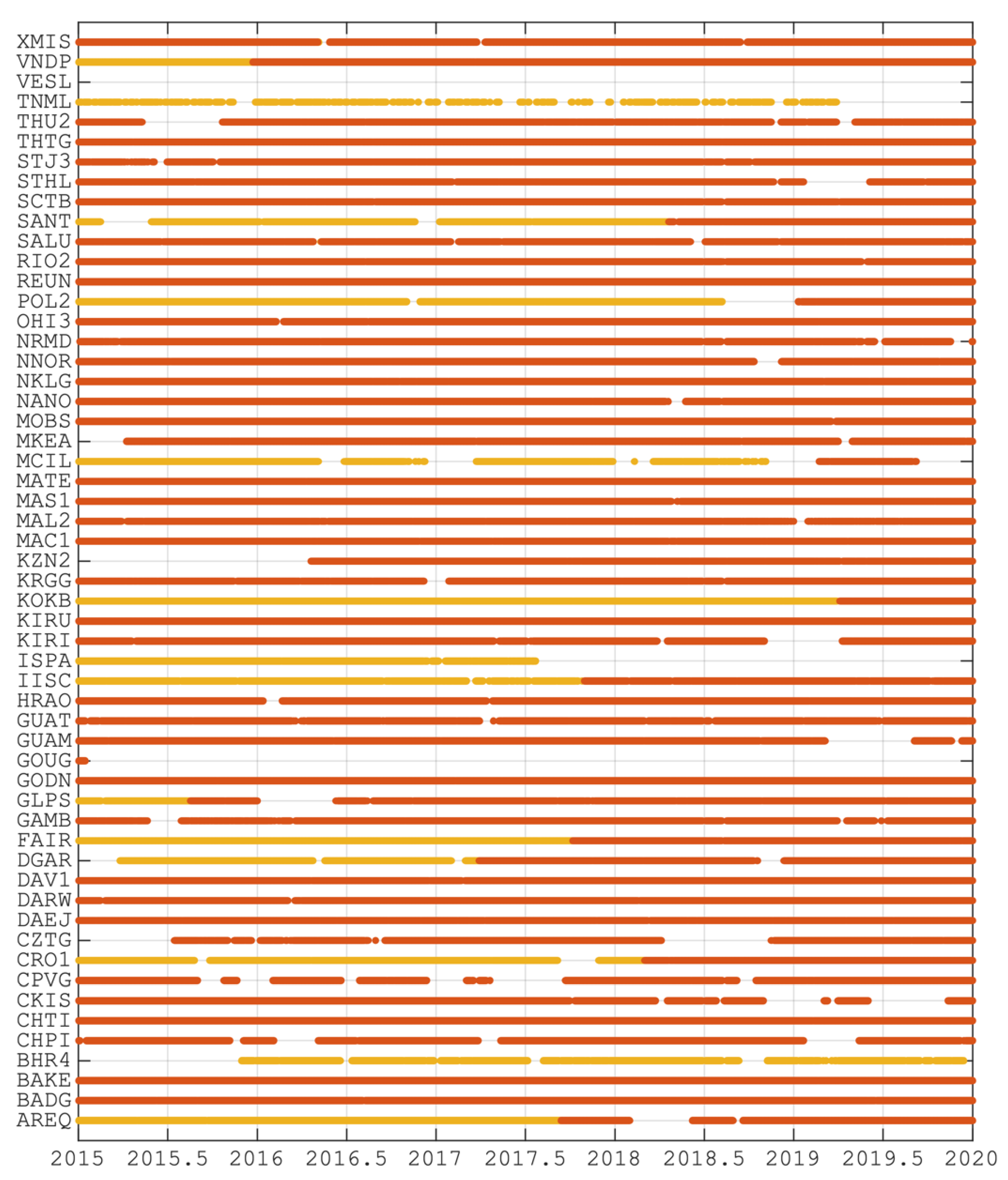
The main steps employed in this study are as follows: first, we select globally distributed stations based on both data quantity and quality; second, we utilize Net_Diff software for Precise Point Positioning, both with and without Ambiguity Resolution and the QOCA platform (Version 1.28), which was developed by the Jet Propulsion Laboratory (JPL) for time series analysis [20,21,22].

2.1. Data Source

The IGS Analysis Center Coordinator has identified 55 main core stations used in the IGS20 reference frame [23]. These core stations are the highest-performing, globally distributed stations used by IGS ACs to align unconstrained global AC solutions (orbit, clock, and position) to the current IGS realization of the ITRF. The availability of observation files for each station across all epochs is depicted in Figure 1. Five stations (BHR4, GOUG, ISPA, TNML, VESL) were excluded due to insufficient observation data, with more than 580 daily observation data (more than 30% of the total daily observation data) missing. Station KZN2 was also excluded because no observation data were available prior to March 2016, preventing a complete time-series analysis. As a result, a total of 49 stations were selected for this study. The spatial distribution of the 55 stations is illustrated in Figure 2, with the six excluded stations indicated in orange.

In this study, we performed PPP-AR on the observation data spanning from 2015.0 to 2020.0. The experiment duration of 5 years exceeds the minimum time span of 2.5 years for constructing a velocity field, as recommended by Blewitt and Lavallée (2002) [2,24]. The orbits, clock, and bias products necessary for PPP-AR are available at the IGS Data Centers [25].

2.2. PPP-AR Strategy

The positioning strategy adopted in this research is detailed in

Table 1. PPP-AR strategies.

Item	Strategies
Satellite system	GPS, Galileo
Data sampling rate	30s
Elevation cutoff angle	7
Observations noise	code: 30 cm, phase: 3 mm
Satellite orbit and clock	IGS Repro3 precise products provided by WUM
Observable-specific bias	IGS Repro3 precise products provided by WUM
Phase center offset	igsR3_2135.atx
Tropospheric delay	Initial value: GPT2w + SAAS + VMF1 remaining wet delay: random walk parameter [27]
Ionospheric delay	Ionosphere-free combination [28]
Ambiguity fixed method	Wide-lane: rounding; narrow-lane: LAMBDA [29]
Earth deformation correction	IERS Conventions 2010 [30,31]

. Precise products from IGS Repro3, along with the corresponding igsR3_2135.atx file, were utilized. These data were provided by WUM AC [25]. The OSB products provided by WUM during this period include data from both the GPS and Galileo systems. Although GLONASS contributes to ITRF solutions to some extent, this analysis focuses on GPS and Galileo, as they enable Ambiguity Resolution and effectively demonstrate the improvements of PPP-AR [26]. The Precise Point Positioning software, Net_Diff (Version 1.17), utilized in this paper, is a high-accuracy positioning software developed by the GNSS Analysis Center at Shanghai Astronomical Observatory. All parameters and algorithms implemented in the software adhere to the standards established by IGS. Net_Diff is capable of performing PPP, multi-station network solutions, and PPP-RTK across multi-GNSS, including GPS, GLONASS, Galileo, BDS, Navic, and QZSS.

2.3. Position Time Series Processing Strategy

The GNSS time series includes both tectonic and non-tectonic signals. Tectonic signals, which are the signals of our interest, represent Earth’s surface displacements or deformations caused by geological processes such as crustal and plate movements. In contrast, non-tectonic signals are unrelated to plate tectonics or other geodynamic phenomena [32]. Accurately extracting tectonic signals from the GNSS time series is a significant challenge, as it requires effectively mitigating the influence of non-tectonic signals and noise in these complex datasets.

The coordinate time series of the selected stations were fitted using the time series model presented in Equation (1) through least squares estimation [33,34].

$$x\left(t\right)=x_0+v·\left(t-t_0\right)+{{\displaystyle \sum }}_i\left[S_i sin\left({\omega }_{i}t\right)+C_i cos\left({\omega }_{i}t\right)\right]+{{\displaystyle \sum }}_k{D}_{k}B\left(t_k^1,t_k^2\right)+{{\displaystyle \sum }}_j{F}_j\left(t\right)$$

(1)

In the above equation, $x\left(t\right)$ represents the station coordinate at epoch $t$. $x_0$ denotes the offset. $v$ represents the velocity. $t$ and $t_0$ correspond to the observation epoch and reference epoch in years, respectively. ${\omega }_i$ represents the period of the sine function or cosine function, where $2\pi$ represents the annual period and $4\pi$ represents the semi-annual period. $S_i$ and $C_i$ are the component amplitudes of the annual and semi-annual variations, respectively. $D_k$ denotes the amplitude of the boxcar function. $B\left(t_k^1,t_k^2\right)$ is characterized by two time-dummy parameters: the start and end times. $F_j$ represents the amplitudes of the remaining nonlinear components.

Equation (1) was implemented in the time-series analysis module of QOCA. The model was conducted for all chosen stations, which accounted for offsets, velocities, and seasonal terms in the coordinate time series. The global geocentric coordinates were transformed into local topocentric coordinates (to facilitate separate analyses of horizontal and vertical components) [14]. Solutions with formal uncertainties or residuals greater than 30 mm in horizontal components, or 60 mm in vertical components, were excluded from the analysis [33].

3. Results and Analysis

A statistical analysis was carried out on the ambiguity fixed rate at the last epoch of each day, which we define as the proportion of successfully fixed solutions.

Figure 3 shows the fixed rate of each station. As shown, the fixed rate of station MKEA was below 85%, and that of station CZTG in 2019 is 86.2%. Due to the station’s location or poor observation data quality, the performance of the float PPP solution deteriorated, ultimately resulting in a lower fixed rate [35]. Consequently, these two stations were excluded from subsequent analyses. For the remaining 47 stations, the fixed rates exceeded 89.7%, with an average fixed rate of 98.13%. Additionally, positioning results for station KIRU were deemed unreliable due to antenna errors after 2019.87 [35]. Ultimately, 46 stations were selected as experimental targets, and the PPP-AR results for these stations are considered robust and reliable.

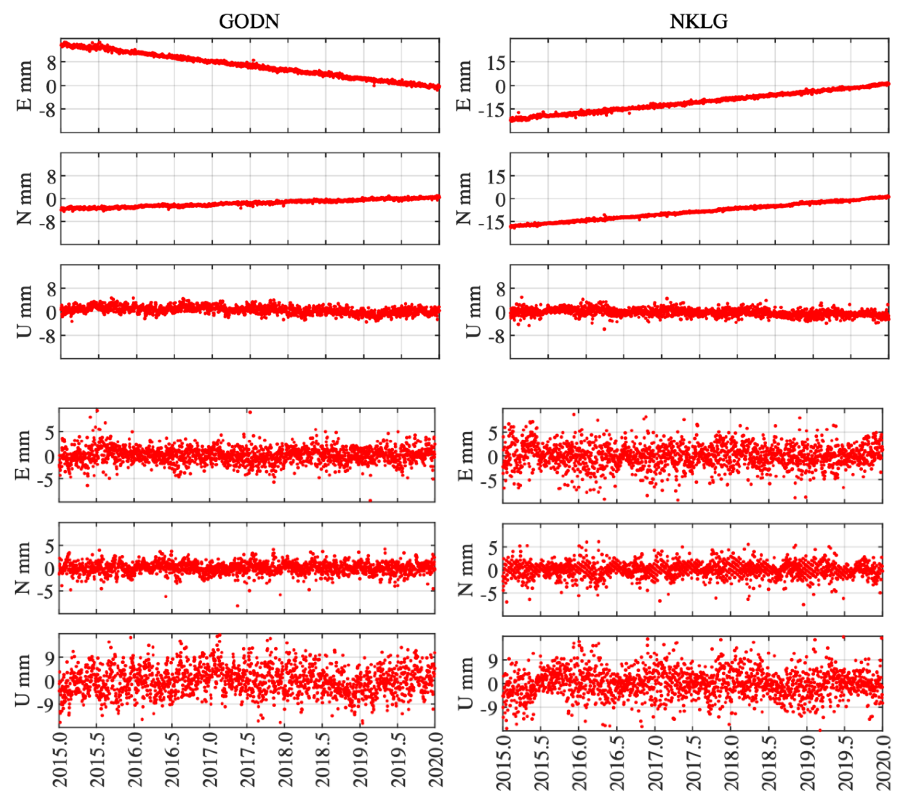
3.1. Station Coordinate

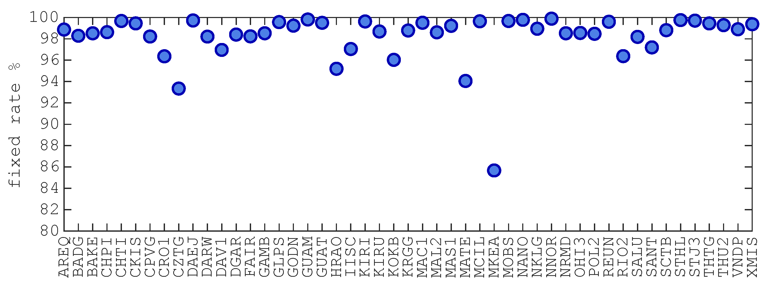
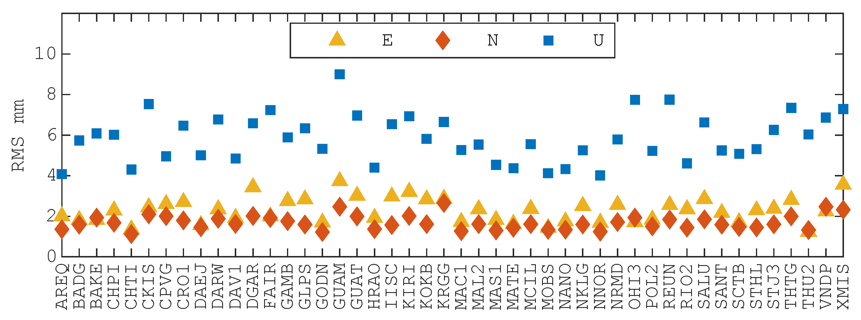
3.1.1. Coordinates Accuracy

Following Precise Point Positioning, an accuracy analysis of the positioning results was conducted. Over long timescales, station movements exhibit slow linear trends, seasonal variations, and, in some cases, co-seismic and post-seismic deformation. To address these factors, we applied model fitting as described in Equation (1) for each station, generating residual time series (daily solutions minus fitting values). Approximately 1.29% of the solutions were excluded from the analysis due to uncertainties or residuals exceeding 30 mm in the horizontal component or 60 mm in the vertical component. The root mean square (RMS) of the residual time series was then computed to assess the accuracy of the PPP-AR-derived solutions. Residuals exceeding three times their RMS were identified as outliers and excluded from the statistical analysis.

Figure 4 presents the coordinate time series for stations GODN and NKLG, as well as the residual time series after model fitting. The top subplots indicate significant linear displacement at both stations, corresponding to the velocities of interest discussed in later sections. After subtracting the fitting values, the RMSs for both stations are within 3 mm in the horizontal direction and 6 mm in the vertical direction.

Figure 5 presents residual RMSs for all stations. The average RMSs across all stations are 2.30 mm, 1.70 mm, and 5.86 mm for the E, N, and U components, respectively. The positioning accuracy of the IGS final products is 2 mm horizontally and 5 mm vertically [36]. The precision achieved in our analysis is nearly equivalent to these reference values; however, it is significantly lower than that of IGS Repro3.

3.1.2. Coordinates Comparison with IGS Repro3

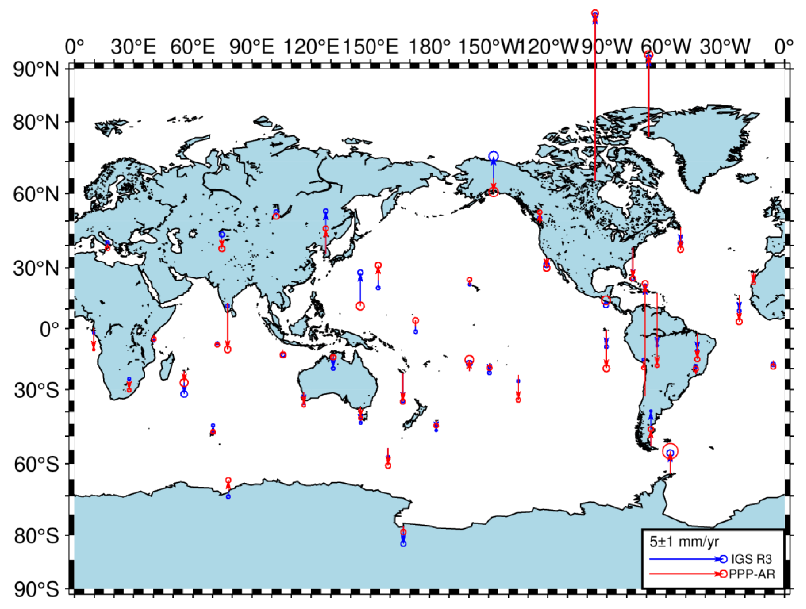
We also compared the daily positioning results derived from PPP-AR solutions with the corresponding IGS Repro3 (referred to as IGS R3 in the following text) coordinates, which were regarded as the true reference values. These differences are defined as relative accuracy.

Using stations GODN and NKLG as representative examples, Figure 6 illustrates the coordinate time series and the corresponding differences between the IGS R3 and PPP-AR solutions for these two stations. From the top panels, it is evident that on a long-term scale, the PPP-AR solutions demonstrate strong consistency with the IGS R3 solutions, as indicated by the close alignment of their trends. Additionally, the IGS R3 solutions exhibit lower dispersion compared to the PPP-AR solutions, reflecting their higher accuracy.

The RMSs of differences between the IGS R3 and PPP-AR solutions for station GODN are 1.49 mm, 1.06 mm, and 3.72 mm in the E, N, and U components, respectively. Similarly, for station NKLG, the RMS of differences are 2.04 mm, 1.15 mm, and 5.39 mm for the E, N, and U components, respectively. This result suggests that there seems to be a significant difference between the two solutions, which may be attributed to differences in processing strategies and models employed by IGS R3 and Net_Diff.

To quantify the discrepancies between the IGS R3 and PPP-AR solutions, we computed the standard deviation (STD) and RMS of the differences for each station, as illustrated in Figure 7. The average STD of the differences are 2.16 mm, 1.26 mm, and 4.26 mm, while the average RMS are 2.37 mm, 1.58 mm, and 5.10 mm for the E, N, and U directions, respectively. The findings indicate the presence of systematic bias in the dataset. To address this issue, we implemented Helmert transformation, a fundamental tool widely used in reference frame alignment, to effectively eliminate the errors and evaluate the consistency between the two solution sets [32].

Table 2. Helmert transformation parameters between IGS R3 and PPP-AR solutions at epoch 2015.0.

	Tx mm	Ty mm	Tz mm	Rx mas	Ry mas	Rz mas	D ppb
	$\dot{\mathit{T}}$x mm/yr	$\dot{\mathit{T}}$y mm/yr	$\dot{\mathit{T}}$z mm/yr	$\dot{\mathit{R}}$x mas/yr	$\dot{\mathit{R}}$y mas/yr	$\dot{\mathit{R}}$z mas/yr	$\dot{\mathit{D}}$ ppb/yr
Value	−1.10 ±0.53	−0.01 ±0.53	−0.25 ±0.53	0.001 ±0.021	−0.002 ±0.021	−0.022 ±0.021	0.38 ±0.08
Trend	0.22 ±0.64	−0.03 ±0.73	0.23 ±0.71	0.001 ±0.012	−0.000 ±0.011	0.002 ±0.024	0.06 ±0.12

presents the Helmert transformation parameters at epoch 2015.0, along with the standard deviations and trends of the parameter time series.

After applying the Helmert transformation, a statistical analysis was conducted on the residuals, referred to as the post-transformation residuals. Figure 8 illustrates the RMSs of post-transformation residuals between IGS R3 and PPP-AR solutions in the E, N, and U components. The average RMSs for all stations are 2.08 mm, 1.34 mm, and 4.65 mm for the E, N, and U directions, respectively. These residuals are roughly equivalent to the formal error of the IGS final products [36], demonstrating the robust agreement between the two datasets.

3.2. Velocity Field

We estimated the station velocities using the model described in Equation (1) and determined the flicker noise level of the series using the simplified formula of Williams (2003), accounting for the uncertainty in the velocity solutions [37]. The results of the uncertainties are shown in Figure 9. Compared to the horizontal components, the uncertainty in the vertical component is approximately three times higher. This observation aligns with the findings of Stylianos Bitharis (2023) [32]. This is due to the imbalance in height observations, which, unlike the nearly balanced horizontal observations, are only available in the upper hemisphere of the observation field.

The average estimated uncertainties in velocity are 0.29 mm/yr, 0.23 mm/yr, and 0.82 mm/yr for the E, N, and U components, respectively. These values are comparable to the formal error of the ITRF horizontal velocity field (0.25 mm/yr) and slightly higher than the formal error reported for the IGS horizontal velocity field 0.2 mm/yr [36,38].

Table A1. Velocity in E directions of selected stations (Unit: mm/yr).

Station	Velocity	Station	Velocity	Station	Velocity	Station	Velocity
AREQ	10.07 ±0.26	FAIR	−7.94 ±0.29	MAL2	26.41 ±0.31	RIO2	5.02 ±0.35
BADG	26.77 ±0.29	GAMB	−67.40 ±0.34	MAS1	16.57 ±0.21	SALU	−3.57 ±0.33
BAKE	−19.15 ±0.23	GLPS	50.51 ±0.41	MATE	23.56 ±0.18	SANT	15.07 ±0.30
CHPI	−3.92 ±0.29	GODN	−14.76 ±0.15	MCIL	−71.57 ±0.46	SCTB	9.21 ±0.24
CHTI	−40.72 ±0.17	GUAM	−6.96 ±0.54	MOBS	19.22 ±0.16	STHL	23.44 ±0.33
CKIS	−62.48 ±0.31	GUAT	2.37 ±0.57	NANO	−8.07 ±0.27	STJ3	−13.87 ±0.36
CPVG	18.53 ±0.44	HRAO	17.23 ±0.22	NKLG	22.36 ±0.18	THTG	−65.86 ±0.22
CRO1	7.65 ±0.27	IISC	42.89 ±0.33	NNOR	38.34 ±0.24	THU2	−22.77 ±0.18
DAEJ	27.83 ±0.16	KIRI	−68.38 ±0.34	NRMD	20.95 ±0.39	VNDP	−41.46 ±0.28
DARW	35.40 ±0.25	KOKB	−62.02 ±0.26	OHI3	15.57 ±0.35	XMIS	40.87 ±0.46
DAV1	−3.02 ±0.22	KRGG	5.11 ±0.20	POL2	27.51 ±0.25
DGAR	47.46 ±0.33	MAC1	−11.88 ±0.21	REUN	17.78 ±0.30

,

Table A2. Velocity in N directions of selected stations (Unit: mm/yr).

Station	Velocity	Station	Velocity	Station	Velocity	Station	Velocity
AREQ	14.42 ±0.18	FAIR	−21.94 ±0.33	MAL2	15.88 ±0.23	RIO2	12.33 ±0.20
BADG	−6.57 ±0.25	GAMB	31.85 ±0.22	MAS1	17.25 ±0.15	SALU	13.23 ±0.20
BAKE	−4.29 ±0.31	GLPS	11.06 ±0.22	MATE	19.53 ±0.18	SANT	15.92 ±0.28
CHPI	−12.69 ±0.24	GODN	4.19 ±0.13	MCIL	24.40 ±0.32	SCTB	−11.36 ±0.18
CHTI	33.00 ±0.14	GUAM	4.36 ±0.33	MOBS	57.35 ±0.19	STHL	18.61 ±0.22
CKIS	−35.40 ±0.36	GUAT	0.65 ±0.36	NANO	−8.10 ±0.18	STJ3	13.46 ±0.23
CPVG	15.27 ±0.41	HRAO	18.16 ±0.16	NKLG	19.19 ±0.12	THTG	33.94 ±0.21
CRO1	13.57 ±0.19	IISC	35.90 ±0.19	NNOR	57.84 ±0.16	THU2	4.81 ±0.16
DAEJ	−10.72 ±0.21	KIRI	31.06 ±0.20	NRMD	45.30 ±0.25	VNDP	24.29 ±0.32
DARW	59.24 ±0.20	KOKB	34.40 ±0.18	OHI3	9.44 ±0.47	XMIS	55.25 ±0.29
DAV1	−5.43 ±0.17	KRGG	−3.80 ±0.19	POL2	4.71 ±0.23
DGAR	32.70 ±0.23	MAC1	33.18 ±0.17	REUN	11.31 ±0.23

and

Table A3. Velocity in U directions of selected stations (Unit: mm/yr).

Station	Velocity	Station	Velocity	Station	Velocity	Station	Velocity
AREQ	−0.44 ±0.57	FAIR	−0.93 ±1.34	MAL2	−0.30 ±0.68	RIO2	1.17 ±0.70
BADG	0.00 ±0.82	GAMB	−1.69 ±0.66	MAS1	−0.71 ±0.52	SALU	−1.73 ±0.75
BAKE	11.33 ±1.00	GLPS	−2.59 ±0.99	MATE	−0.30 ±0.60	SANT	7.64 ±0.82
CHPI	0.35 ±0.76	GODN	−2.09 ±0.77	MCIL	0.99 ±0.87	SCTB	−0.41 ±0.80
CHTI	−0.33 ±0.62	GUAM	−0.29 ±1.15	MOBS	−0.76 ±0.57	STHL	−0.42 ±0.77
CKIS	0.76 ±1.29	GUAT	−0.05 ±1.24	NANO	0.72 ±0.67	STJ3	−1.51 ±0.87
CPVG	−1.78 ±0.81	HRAO	−0.63 ±0.52	NKLG	−1.47 ±0.38	THTG	−0.29 ±0.75
CRO1	−4.90 ±0.60	IISC	−3.15 ±0.91	NNOR	−0.90 ±0.56	THU2	5.55 ±1.17
DAEJ	1.71 ±0.71	KIRI	0.37 ±0.83	NRMD	−1.93 ±0.75	VNDP	−0.69 ±0.96
DARW	−0.21 ±0.78	KOKB	0.31 ±0.63	OHI3	1.53 ±2.12	XMIS	−0.38 ±0.87
DAV1	0.73 ±0.71	KRGG	0.20 ±0.69	POL2	−0.65 ±0.82
DGAR	−0.13 ±0.64	MAC1	−1.18 ±0.78	REUN	−0.78 ±1.12

in Appendix A summarize the station velocities (in mm/year) and their associated uncertainties for the selected sites. The data reveal no consistent pattern in the magnitude of station movements within the same direction. However, significant differences are evident between directions. For example, velocities in the U direction are notably smaller than those in the E and N directions, while the associated uncertainties in the U direction are considerably higher. These differences are primarily attributed to the pronounced horizontal motion of tectonic plates and the nonlinear variability in vertical movements [2]. Specifically, the horizontal velocities of stations in the Atlantic region are relatively large, with an average exceeding 20 mm/year, whereas the vertical velocities are substantially smaller, averaging less than 0.5 mm/year.

To further validate the reliability of the estimated velocity field, we compared the velocity solutions derived from PPP-AR with those from IGS R3. It is important to note that the IGS velocity field product is derived from GNSS observations spanning from Day 002 in 1995 to Day 001 in 2021, whereas the velocity field presented in this study is based on GNSS observations from Day 001 in 2015 to Day 001 in 2020. Consequently, a direct comparison of the two velocity solutions would be inappropriate due to the different observation time spans.

To address this, we performed model fitting on the station coordinates provided by IGS R3 (2015.0–2020.0) to derive a velocity solution, which was subsequently used as the reference “true” velocity. Figure 10 and Figure 11 illustrate the horizontal and vertical velocity components from both IGS R3 and PPP-AR solutions. The ellipses represent the 95% confidence interval.

The mean velocity differences between IGS R3 and PPP-AR solutions are 0.32 mm/yr, 0.19 mm/yr, and 0.67 mm/yr for the E, N, and U components, respectively. Notably, the differences in the horizontal velocity components are comparable to the formal errors of the ITRF velocity field (0.25 mm/yr in the horizontal component) but slightly exceed those of the IGS velocity field (0.2 mm/yr in the horizontal component). For the vertical velocity component, the differences are smaller than the formal errors of both the ITRF and IGS velocity fields. These findings confirm that the PPP-AR-derived velocity field exhibits high accuracy and reliability, particularly when compared with globally recognized reference velocity solutions.

3.3. Seasonal Term

Beyond linear trends, seasonal terms, predominantly in the form of annual and semi-annual cycles, are commonly observed in the GNSS coordinate time series [33]. Accurately retrieving seasonal signals from the GNSS time series not only improves the reliability of the GNSS time series but also plays a crucial role in analyzing various geophysical phenomena [39,40]. These seasonal terms, particularly the annual signal, often vary across ACs due to differences in processing strategies and models, making them important for further investigation.

We estimated the seasonal amplitudes of the station coordinates from both IGS R3 and PPP-AR solutions. The amplitude $A$ is defined as [41]

$$A=\sqrt{{S_i}^2+{C_i}^2}$$

(2)

where $S_i$ and $C_i$ represent the component amplitudes, as defined in Equation (1).

Figure 12 and Figure 13 illustrate the annual and semi-annual amplitudes for both solutions, respectively. The average differences in annual amplitudes between IGS R3and PPP-AR solutions are 0.36 mm, 0.27 mm, and 0.68 mm for the E, N, and U components, respectively. Similarly, the average differences in semi-annual amplitudes are 0.31 mm, 0.12 mm, and 0.43 mm for the E, N, and U directions, respectively. Except for a few stations, the seasonal amplitudes derived from the two solutions show strong consistency across the majority of stations, which is much lower than the difference between four representative GPS time-series products (JPL, SOPAC, MEaSUREs, NGL) [42]. This is because we have added Galileo to perform PPP-AR, and it does not have an orbital period aliasing with a sidereal day, thus producing a more significant annual periodic position signal. This observation is consistent with the conclusions of Dong et al. (2002) and Rebischung et al. (2024) [4,41]. If the GLONASS system is additionally included, the annual periodic amplitude will be partially suppressed due to the complexity of its different orbital period. This result further validates that the PPP-AR method effectively extracts seasonal signals that are comparable to those obtained from IGS R3 solutions.

3.4. Coordinate Prediction from Velocity and Seasonal Terms

One of the purposes of estimating station velocities and seasonal terms is to enable the interpolation and prediction of station coordinates for any epoch, based on known coordinates, velocities, and seasonal terms at a reference epoch. As such, the accuracy of velocity and seasonal terms estimates plays a pivotal role in determining the accuracy of coordinate predictions over time. To further evaluate the accuracy and reliability of the PPP-AR velocity field, we analyzed the accuracy of the predicted coordinates calculated using the estimated velocity and seasonal terms.

Using IGS R3 solutions on the last day of 2019 as the initial value, we calculated the coordinates for all epochs from 2020.0 to 2025.0 using the velocities and seasonal terms derived from PPP-AR and IGS R3. We then compared the predicted coordinates with the corresponding IGS R3 solutions (before GPS week 2238, 27 November 2022) and CODE solutions (after GPS week 2238). Hereafter, both IGS R3 and CODE solutions are collectively referred to as IGS solutions.

Table 3. RMS values of differences between IGS coordinates and the coordinates derived from PPP-AR and IGS R3 velocity (Unit: mm).

Year	Coordinates Derived from PPP-AR			Coordinates Derived from IGS R3
	E	N	U	E	N	U
2020	2.23	2.24	6.40	2.11	2.12	5.86
2021	2.53	2.31	6.57	2.53	2.27	6.07
2022	3.28	2.76	7.25	3.24	2.83	7.01
2023	4.04	5.60	7.79	4.15	5.64	7.71
2024	4.84	5.68	8.74	4.81	5.74	8.31

provides the RMS values of annual differences between the IGS solutions, and those predicted coordinates derived from the velocities and seasonal terms of PPP-AR and IGS.

The minimal differences between the predicted coordinates derived from the two velocity fields and seasonal terms demonstrate the reliability of the PPP-AR-estimated velocity field and seasonal terms. In addition, over a two-year period, the horizontal coordinate accuracy obtained using the velocities and seasonal terms is commendable, with differences within 3 mm horizontally and 6 mm vertically. However, the differences between the IGS solutions and the predicted coordinates increase incrementally over the years. By the fifth year, the differences reach 6 mm horizontally and 9 mm vertically. This trend highlights the limitations of coordinate prediction based solely on velocity and seasonal terms, emphasizing the necessity for periodic updates of the reference frame to maintain high accuracy.

4. Discussion

To evaluate the advantages of PPP-AR over PPP, we also conducted static PPP solutions for the aforementioned stations, covering the same time period from 2015.0 to 2020.0. The methodology outlined in Section 2 was consistently applied across all analyses, ensuring a uniform and objective evaluation process. Similarly to the previous content, we performed accuracy analysis on the positioning results, including station coordinates, velocity field, and seasonal terms.

During the model fitting of PPP solutions, approximately 2.68% of the solutions—higher than that of PPP-AR—were excluded from the analysis due to uncertainties or residuals exceeding 30 mm in the horizontal component or 60 mm in the vertical component. The average RMSs of the residual time series for all stations estimated using PPP are 2.64 mm, 1.72 mm, and 5.93 mm in the E, N, and U directions, respectively, as shown in

Table 4. RMS values of residual time series and post-transformation residuals of two solutions (Unit: mm).

Strategy	Residual Time Series			Post-Transformation Residuals
	E	N	U	E	N	U
PPP	2.64	1.72	5.93	2.47	1.37	4.72
PPP-AR	2.30	1.70	5.86	2.08	1.34	4.65

. The average RMSs of the residual time series estimated using PPP-AR, as presented in Section 3.1.1, are also listed in Table 4, with values of 2.30 mm, 1.70 mm, and 5.86 mm in the E, N, and U directions, respectively. Clearly, the standard deviation of the residual time series for the PPP-AR solution is smaller, particularly in the E direction, indicating higher accuracy. Accordingly, compared to float solutions, Ambiguity Resolution enhances the accuracy of the coordinate in the E direction.

Similarly to the approach in Section 3.1.2, we also applied Helmert transformation between PPP solutions and IGS R3 solutions.

Table 5. Helmert transformation parameters between IGS R3 and PPP solutions at epoch 2015.0.

	Tx mm	Ty mm	Tz mm	Rx mas	Ry mas	Rz mas	D ppb
	$\dot{\mathit{T}}$x mm/yr	$\dot{\mathit{T}}$y mm/yr	$\dot{\mathit{T}}$z mm/yr	$\dot{\mathit{R}}$x mas/yr	$\dot{\mathit{R}}$y mas/yr	$\dot{\mathit{R}}$z mas/yr	$\dot{\mathit{D}}$ ppb/y
Value	−1.18 ±0.49	0.30 ±0.49	−0.10 ±0.49	0.003 ±0.019	−0.002 ±0.020	−0.023 ±0.019	0.42 ±0.08
Trend	0.23 ±0.68	−0.06 ±0.75	0.23 ±0.72	0.001 ±0.012	0.000 ±0.012	0.002 ±0.026	0.06 ±0.12

presents the Helmert transformation parameters between PPP solutions and IGS R3 solutions at epoch 2015.0, along with the standard deviations and trends of the parameter time series. By comparing Table 2 and Table 5, most of the transformation parameters between PPP-AR and IGS R3 are smaller. Notably, the relatively large STD in Table 2 can be attributed to the inclusion of both float and fixed solutions, which is understandable.

A statistical analysis of the post-transformation residual was conducted. Table 4 also presents the post-transformation residuals between the IGS R3 and PPP solutions, as well as between the IGS R3 and PPP-AR solutions mentioned in Section 3.1.2, across all stations for the E, N, and U components, respectively. The PPP-AR solution shows an improvement in the horizontal direction compared to the PPP solution, particularly in the east direction, with an improvement of approximately 0.3 mm. This result is aligned with the results of Geng et al. [43]. However, the improvement is not as significant as Geng et al., possibly due to inconsistencies in the data time spans. Clearly, the post-transformation residuals between PPP-AR and IGS R3 solutions are smaller, which also indicates a higher relative accuracy for the PPP-AR solutions.

The station velocities and their uncertainties derived from the PPP solution were also estimated. The uncertainties derived from PPP, PPP-AR, and IGS R3 are presented in

Table 6. Uncertainties of velocity and velocity difference (Unit: mm/yr).

Strategy	Uncertainty of Velocity			Velocity Difference
	E	N	U	E	N	U
PPP	0.31	0.23	0.86	0.37	0.19	0.69
PPP-AR	0.29	0.23	0.82	0.32	0.19	0.67
IGS R3	0.18	0.18	0.58	/	/	/

. The velocity difference between PPP/PPP-AR and IGS R3 is also listed in Table 6. It can be observed that the uncertainties estimated by the three solutions increase in the following order: IGS R3 exhibits the smallest uncertainty, followed by PPP-AR, with PPP showing the biggest uncertainty. Notably, both the estimated velocity uncertainties from PPP-AR and PPP solutions are of a similar order of magnitude to the form error of the ITRF and IGS horizontal velocity fields. Compared to PPP, the velocities estimated by PPP-AR are closer to those estimated by IGS, particularly in the east direction. Overall, from the perspective of velocity estimation, PPP-AR aligns more closely with IGS than PPP.

Table 7. Seasonal term amplitude difference between PPP/PPP-AR and IGS R3 (Unit: mm).

Strategy	Annual			Semi-Annual
	E	N	U	E	N	U
PPP	0.31	0.27	0.68	0.40	0.12	0.43
PPP-AR	0.36	0.27	0.68	0.31	0.12	0.43

presents the seasonal term amplitude differences between the PPP/PPP-AR and IGS R3 solutions. As shown in the table, compared to the differences with IGS R3, the difference between PPP/PPP-AR solutions is negligible, with only a slight variation observed in the east direction. In terms of seasonal term estimation, Ambiguity Resolution has no significant impact.

5. Conclusions

In this study, we retrieved long-term velocity fields and seasonal terms from PPP-AR solutions rather than from network solutions, thereby laying the foundation for future maintenance and densification of the reference frame. The data used in this study are GNSS observations from 46 uniformly distributed stations across the globe, spanning the period from 2015.0 to 2020.0. We conducted analyses of coordinate accuracy, velocity field accuracy, and seasonal term accuracy based on the results of PPP-AR. The key findings are as follows:

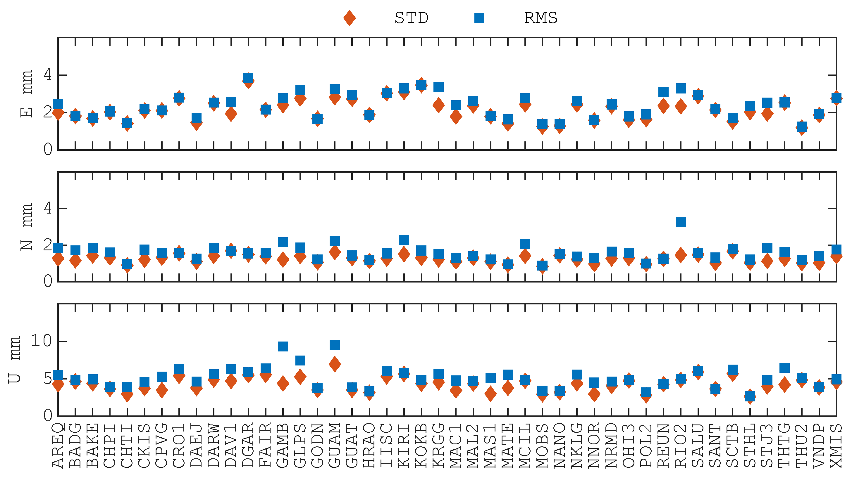
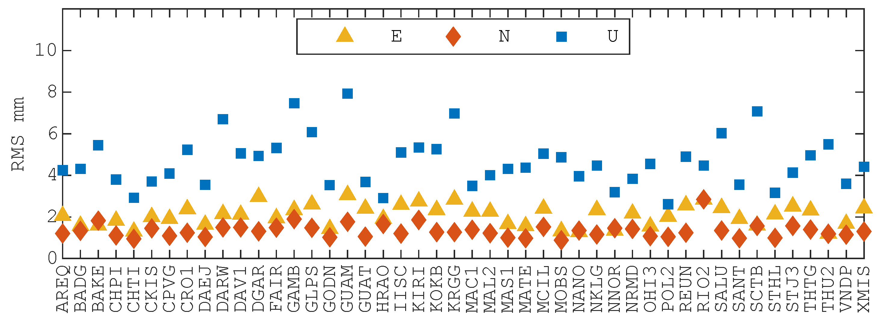
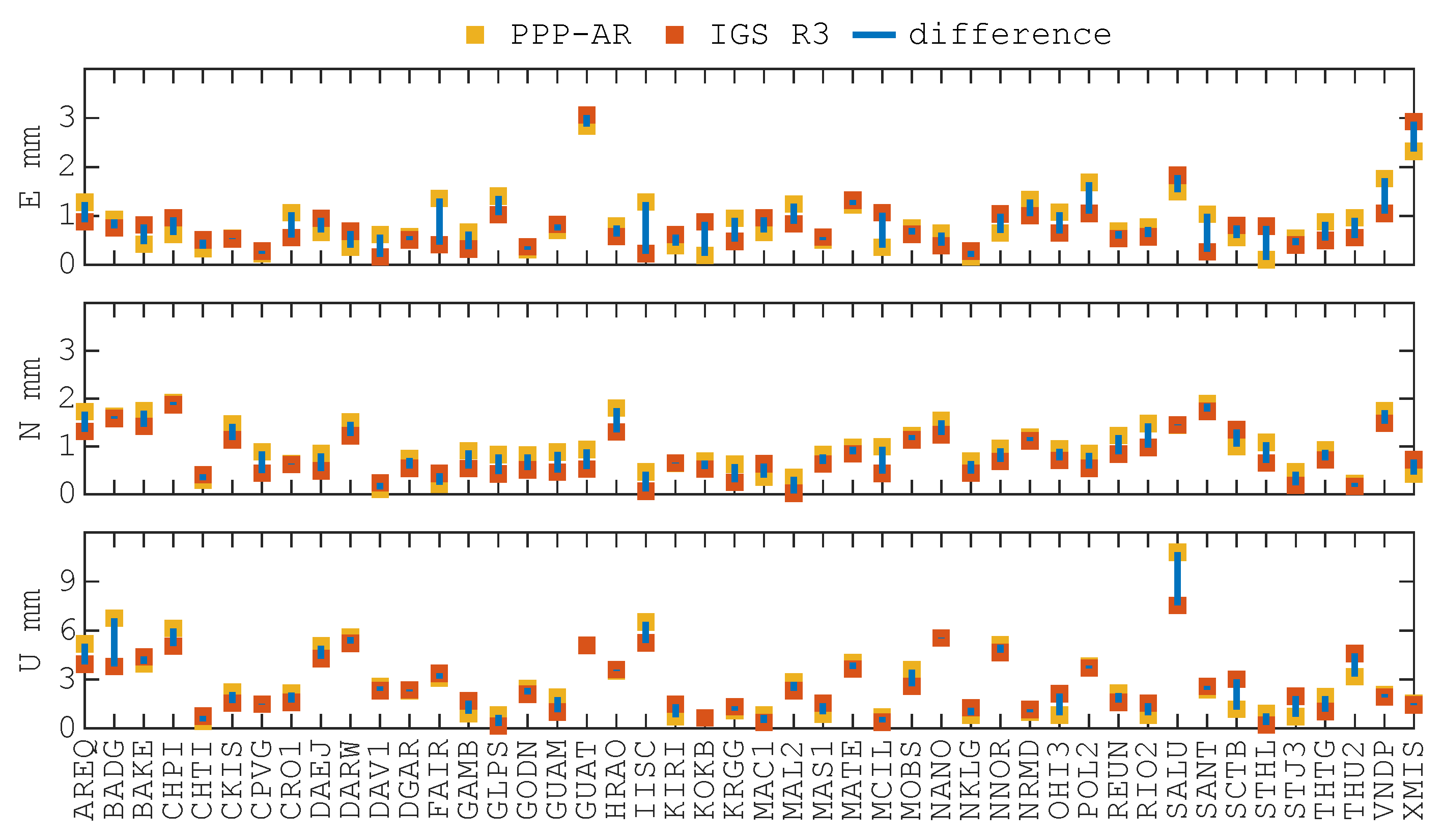
• The average RMS values of residual time series for all stations are within 3 mm in the horizontal direction and within 6 mm in the vertical direction. The average RMSs of the difference between IGS R3 and PPP-AR solutions, after applying Helmert transformation to all stations, are almost within 2 mm in the horizontal direction and within 5 mm in the vertical direction.
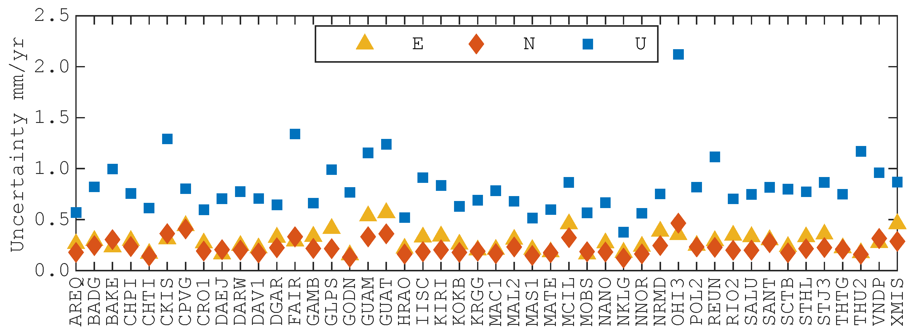
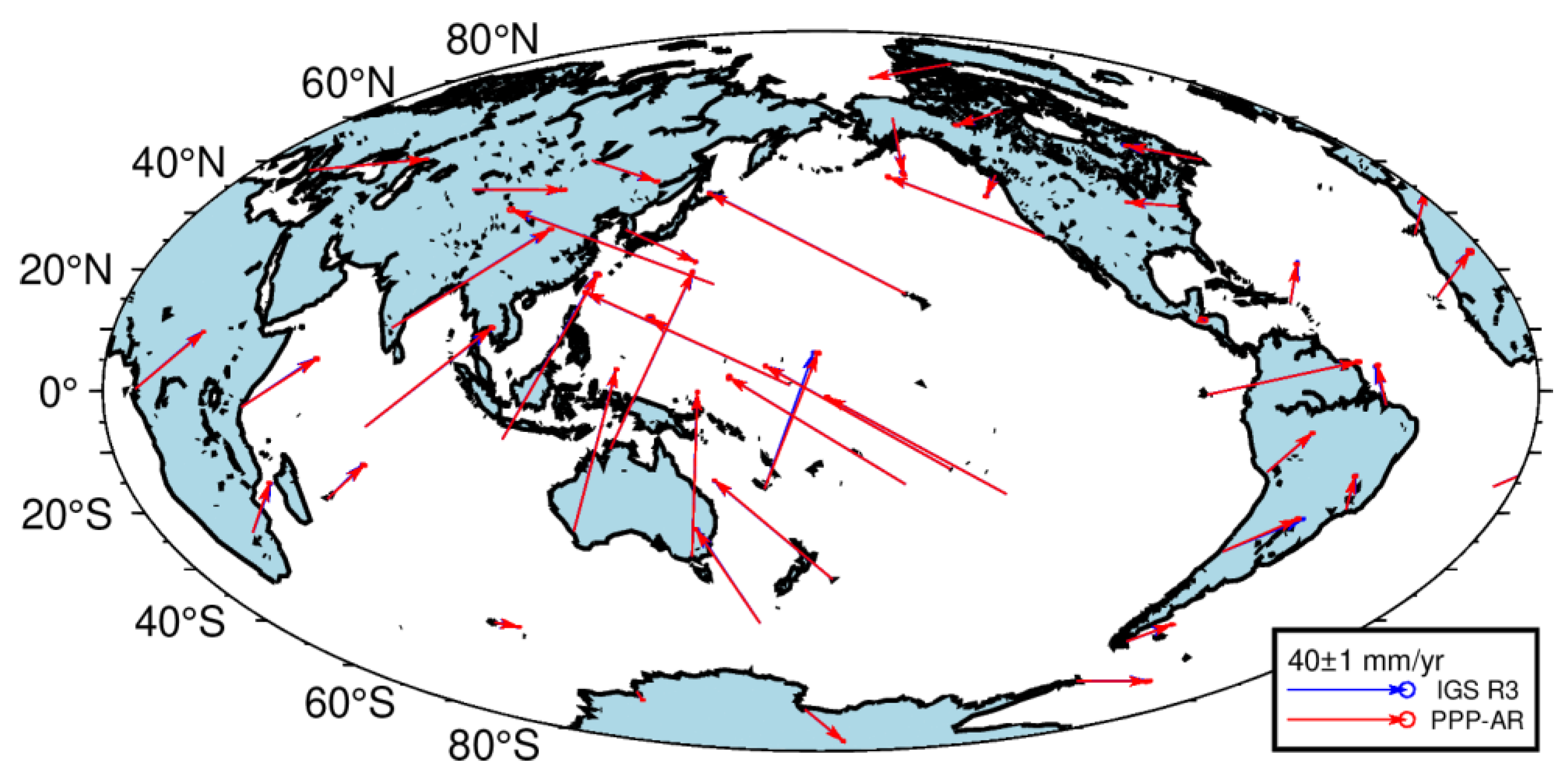
• The uncertainty of velocity derived from PPP-AR solutions is within 0.3 mm/yr for the horizontal direction and 0.9 for the vertical direction. The mean velocity difference between IGS R3 and PPP-AR solutions is within 0.40 mm/yr for horizontal components and within 0.70 mm/yr for vertical components.
• The average annual amplitude differences are within 0.90 mm for all three directions, while the average semi-annual amplitude differences are within 0.50 mm.

In summary, the internal and relative precision of PPP-AR solutions is approximately equivalent to the formal error of IGS final products. The PPP-AR solutions’ fitting velocity uncertainty and the difference between PPP-AR and IGSR3 are nearly equal to the formal error of the ITRF horizontal velocity field and slightly exceed the formal error of the IGS horizontal velocity field. Except for a few stations with notable discrepancies, the seasonal amplitudes of the remaining stations exhibit strong consistency. Compared to PPP solutions, PPP-AR solutions achieve improvements in both coordinate and velocity accuracy, especially in the east component. The consistency between the IGS Repro3 orbit/clock combination and the IGS Repro3 position solutions is relatively high. Additionally, PPP-AR is highly efficient in computation and flexible in processing, making it fully capable of supporting the maintenance and densification of the reference frame.

References

1. Zeng, Y. GPS Velocity Field of the Western United States for the 2023 National Seismic Hazard Model Update. Seismol. Res. Lett. 2022, 93, 3121–3134. [Google Scholar] [CrossRef]
2. García-Armenteros, J.A. Topo-Iberia CGPS network: A new 3D crustal velocity field in the Iberian Peninsula and Morocco based on 11 years (2008–2019). GPS Solut. 2023, 27, 155. [Google Scholar] [CrossRef]
3. Altamimi, Z.; Rebischung, P.; Collilieux, X.; Métivier, L.; Chanard, K. ITRF2020: An augmented reference frame refining the modeling of nonlinear station motions. J. Geod. 2023, 97, 47. [Google Scholar] [CrossRef]
4. Rebischung, P.; Altamimi, Z.; Métivier, L.; Collilieux, X.; Gobron, K.; Chanard, K. Analysis of the IGS contribution to ITRF2020. J. Geod. 2024, 98, 49. [Google Scholar] [CrossRef]
5. Wang, H.; Dang, Y.M.; Hou, Y.F.; Mi, J.Z.; Wang, J.X.; Bai, G.X.; Cheng, Y.Y.; Zhang, S.J. Rapid and precise solution of the whole network of thousands of stations in China based on PPP network solution by UPD fixed technology. Acta Geod. Cartogr. Sin. 2020, 49, 278–291. [Google Scholar]
6. Zumberge, J.F.; Heflin, M.B.; Jefferson, D.C.; Watkins, M.M.; Webb, F.H. Precise Point Positioning for the Efficient and Robust Analysis of GPS Data from Large Networks. J. Geophys. Res. 1997, 102, 5005–5017. [Google Scholar] [CrossRef]
7. Tu, R. Fast determination of displacement by PPP velocity estimation. Geophys. J. Int. 2013, 196, 1397–1401. [Google Scholar] [CrossRef]
8. Chen, J.; Zhang, Y.; Yu, C.; Wang, A.; Song, Z.; Zhou, J. Models and Performance of SBAS and PPP of BDS. Satell. Navig. 2022, 3, 4. [Google Scholar] [CrossRef]
9. Wang, A.; Zhang, Y.; Chen, J.; Liu, X.; Wang, H. Regional Real-Time between-Satellite Single-Differenced Ionospheric Model Establishing by Multi-GNSS Single-Frequency Observations: Performance Evaluation and PPP Augmentation. Remote Sens. 2024, 16, 1511. [Google Scholar] [CrossRef]
10. Su, K.; Jiao, G. Estimation of BDS Pseudorange Biases with High Temporal Resolution: Feasibility, Affecting Factors, and Necessity. Satell. Navig. 2023, 4, 17. [Google Scholar] [CrossRef]
11. Ge, M.; Gendt, G.; Rothacher, M.A.; Shi, C.; Liu, J. Resolution of GPS carrier-phase ambiguities in Precise Point Positioning (PPP) with daily observations. J. Geod. 2008, 82, 389–399. [Google Scholar] [CrossRef]
12. Guo, J.; Geng, J.; Wang, C. Impact of the Third Frequency GNSS Pseudorange and Carrier Phase Observations on Rapid PPP Convergences. GPS Solut. 2021, 25, 30. [Google Scholar] [CrossRef]
13. Rabah, M.; Zedan, Z.; Ghanem, E.; Awad, A.; Sherif, A. Study the feasibility of using PPP for establishing CORS network. Arab. J. Geosci. 2016, 9, 613. [Google Scholar] [CrossRef]
14. Arias-Gallegos, A.; Borque-Arancón, M.J.; Gil-Cruz, A.J. Present-Day Crustal Velocity Field in Ecuador from cGPS Position Time Series. Sensors 2023, 23, 3301. [Google Scholar] [CrossRef]
15. Ogutcu, S.; Alcay, S.; Duman, H.; Ozdemir, B.N.; Konukseven, C. Static and kinematic PPP-AR performance of low-cost GNSS receiver in monitoring displacements. Adv. Space Res. 2023, 71, 4795–4808. [Google Scholar] [CrossRef]
16. Nguyen, N.L.; Dang, V.C.B.; Pham, C. Determine Tectonic Motion Velocities of Some Vietnam CORSs Computed from PPP Coordinates When Using IGS and CNES Products. In Proceedings of the Third International Conference on Sustainable Civil Engineering and Architecture. ICSCEA 2023; Reddy, J.N., Wang, C.M., Luong, V.H., Le, A.T., Eds.; Lecture Notes in Civil Engineering; Springer: Singapore, 2024; Volume 442. [Google Scholar] [CrossRef]
17. Chen, G.; Wei, N.; Tao, J.; Zhao, Q. Comparison between GPS network analysis with undifferenced and double differenced integer ambiguity resolution: A practical perspective. Adv. Space Res. 2024, 74, 582–595. [Google Scholar] [CrossRef]
18. Bock, Y.; Fang, P.; Knox, A.; Sullivan, A.; Jiang, S.; Guns, K.; Golriz, D. Extended Solid Earth Science ESDR System (ES3): Algorithm Theoretical Basis Document (ATBD). Available online: http://garner.ucsd.edu/pub/measuresESESES_products/ATBD/ESESES-ATBD.pdf (accessed on 10 February 2025).
19. Geng, J.; Yan, Z.; Wen, Q.; Männel, B.; Masoumi, S.; Loyer, S.; Mayer-Gürr, T.; Schaer, S. Integrated satellite clock and code/phase bias combination in the third IGS reprocessing campaign. GPS Solut. 2024, 28, 150. [Google Scholar] [CrossRef]
20. GNSS Analysis Center at Shanghai Astronomical Observatory. Net_Diff ver.1.16 Manual. Available online: http://202.127.29.4/shao_gnss_ac/ (accessed on 10 February 2025).
21. Zhang, Y.Z.; Chen, J.P.; Gong, X.Q.; Chen, Q. The update of BDS-2 TGD and its impact on positioning. Adv. Space Res. 2020, 65, 2645–2661. [Google Scholar] [CrossRef]
22. Dong, D.N.; Fang, P.; Bock, Y.; Webb, F.; Prawirodirdjo, L.; Kedar, S.; Jamason, P. Spatiotemporal Filtering Using Principal Component Analysis and Karhunen-Loeve expansion approaches for regional GPS network analysis. J. Geophys. Res. 2006, 111, B03405. [Google Scholar] [CrossRef]
23. International GNSS Service. Available online: ftp://igs-rf.ign.fr/pub/IGS20/IGS20_core.txt (accessed on 10 February 2025).
24. Blewitt, G.; Lavallée, D. Effect of annual signals on geodetic velocity. J. Geophys. Res. Solid Earth 2002, 107, 2068. [Google Scholar] [CrossRef]
25. Geng, J.H.; Yan, Z.; Wen, Q. Multi-GNSS Satellite Clock and Bias Product Combination: The Third IGS Reprocessing Campaign. Geomat. Inf. Sci. Wuhan Univ. 2023, 48, 1070–1081. [Google Scholar] [CrossRef]
26. Geng, J.H.; Chen, X.Y.; Pan, Y.X.; Zhao, Q.L. A modified phase clock/bias model to improve PPP ambiguity resolution at Wuhan University. J. Geod. 2019, 93, 2053–2067. [Google Scholar] [CrossRef]
27. Wang, J.X.; Chen, J.P. Development and application of GPS precise positioning software. J. Tongji Univ. (Nat. Sci.) 2011, 39, 764–767. [Google Scholar]
28. Zhang, X.H.; Ren, X.D.; Guo, F. Influence of higher-order ionospheric delay correction on static precise point positioning. Geomat. Inf. Sci. Wuhan Univ. 2013, 38, 883–887. [Google Scholar] [CrossRef]
29. Geng, J.; Meng, X.; Dodson, A.H.; Teferle, F.N. Integer Ambiguity Resolution in Precise Point Positioning: Method Comparison. J. Geod. 2010, 84, 569–581. [Google Scholar] [CrossRef]
30. Petit, G.; Luzum, B. IERS Conventions Centre. IERS Technical Note No. 36. Available online: https://www.iers.org/SharedDocs/Publikationen/EN/IERS/Publications/tn/TechnNote36/tn36.pdf?__blob=publicationFile&v=1 (accessed on 10 February 2025).
31. Duman, H. GNSS-specific characteristic signals in power spectra of multi-GNSS coordinate time series. Adv. Space Res. 2024, 63, 1234–1245. [Google Scholar] [CrossRef]
32. Bitharis, S. GPS data analysis and geodetic velocity field investigation in Greece, 2001–2016. GPS Solut. 2023, 27, 16. [Google Scholar] [CrossRef]
33. Wang, R.Y.; Chen, J.P.; Dong, D.N.; Tan, W.J.; Liao, X.H. Regional GNSS Common Mode Error Correction to Refine the Global Reference Frame. Remote Sens. 2024, 16, 4469. [Google Scholar] [CrossRef]
34. Chen, B.Z.; Bian, J.W.; Ding, K.H.; Wu, H.C.; Li, H.W. Extracting Seasonal Signals in GNSS Coordinate Time Series via Weighted Nuclear Norm Minimization. Remote Sens. 2020, 12, 2027. [Google Scholar] [CrossRef]
35. International GNSS Service. Available online: https://files.igs.org/pub/station/log/ (accessed on 10 February 2025).
36. International GNSS Service. Available online: https://igs.org/products/#about (accessed on 10 February 2025).
37. Williams, S.D.P. The Effect of Coloured Noise on the Uncertainties of Rates Estimated from Geodetic Time Series. J. Geod. 2003, 76, 483–494. [Google Scholar] [CrossRef]
38. Altamimi, Z.; Métivier, L.; Rebischung, P.; Collilieux, X.; Chanard, K.; Barnéoud, J. ITRF2020 plate motion model. Geophys. Res. Lett. 2023, 50, e2023GL106373. [Google Scholar] [CrossRef]
39. Davis, J.L.; Wernicke, B.P.; Tamisiea, M.E. On seasonal signals in geodetic time series. J. Geophys. Res. Solid Earth 2012, 117, B01403. [Google Scholar] [CrossRef]
40. Klos, A.; Olivares, G.; Teferle, F.N.; Hunegnaw, A.; Bogusz, J. On the combined effect of periodic signals and colored noise on velocity uncertainties. GPS Solut. 2018, 22, 1. [Google Scholar] [CrossRef]
41. Dong, D.; Fang, P.; Bock, Y.; Cheng, M.K.; Miyazaki, S. Anatomy of apparent seasonal variations from GPS-derived site position time series. J. Geophys. Res. 2001, 107, 2075. [Google Scholar] [CrossRef]
42. Wang, S.Y.; Li, J.; Chen, J.; Hu, X.G. Uncertainty Assessments of Load Deformation from Different GPS Time Series Products, GRACE Estimates and Model Predictions: A Case Study over Europe. Remote Sens. 2021, 13, 2765. [Google Scholar] [CrossRef]
43. Geng, J.; Chen, X.Y.; Pan, Y.X.; Mao, S.; Li, C.; Zhou, J.; Zhang, K. PRIDE PPP-AR: An open-source software for GPS PPP ambiguity resolution. GPS Solut. 2019, 23, 91. [Google Scholar] [CrossRef]
Figure 1. Data availability of 55 core IGS stations. The orange dots indicate that the observation data only includes GPS system, while the red dots indicate that the observation data includes multiple systems.
Remotesensing 17 01183 g001
Figure 2. Distribution of 55 selected IGS stations. The orange triangles are six exclusion stations.
Remotesensing 17 01183 g002
Figure 3. Ambiguity fixed rate of each station.
Remotesensing 17 01183 g003
Figure 4. Position and residuals time series of GODN and NKLG (the top subplots depict the station coordinates, while the bottom subplots show the residuals).
Remotesensing 17 01183 g004
Figure 5. RMS of residual time series of PPP-AR solutions of each station.
Remotesensing 17 01183 g005
Figure 6. Coordinate and difference time series between IGS R3 and PPP-AR solutions for stations GODN and NKLG. (Top panels: blue dots represent IGS R3 solutions and red dots represent PPP-AR solutions. Bottom panels: green dots represent the difference time series).
Remotesensing 17 01183 g006
Figure 7. Statistical summary of the differences between IGS R3 and PPP-AR solutions.
Remotesensing 17 01183 g007
Figure 8. RMS of post-transformation residuals between IGS R3 and PPP-AR solutions of each station.
Remotesensing 17 01183 g008
Figure 9. Uncertainty of velocity estimation.
Remotesensing 17 01183 g009
Figure 10. Horizontal velocity derived from IGS R3 and PPP-AR solutions.
Remotesensing 17 01183 g010
Figure 11. Vertical velocity derived from IGS R3 and PPP-AR solutions.
Remotesensing 17 01183 g011
Figure 12. Annual amplitude of IGS R3 and PPP-AR solutions. The orange boxes represent the amplitudes derived from the PPP-AR solution, while the red boxes represent the amplitudes derived from the IGS R3 solution. The blue line illustrates the difference between the two.
Remotesensing 17 01183 g012
Figure 13. Semi-annual amplitude of IGS R3 and PPP-AR solutions. The orange boxes represent the amplitudes derived from the PPP-AR solution, while the red boxes represent the amplitudes derived from the IGS R3 solution. The blue line illustrates the difference between the two.
Remotesensing 17 01183 g013