BathyFormer: A Transformer-Based Deep Learning Method to Map Nearshore Bathymetry with High-Resolution Multispectral Satellite Imagery

Abstract

Accurate mapping of nearshore bathymetry is essential for coastal management, navigation, and environmental monitoring. Traditional bathymetric mapping methods such as sonar surveys and LiDAR are often time-consuming and costly. This paper introduces BathyFormer, a novel vision transformer- and encoder-based deep learning model designed to estimate nearshore bathymetry from high-resolution multispectral satellite imagery. This methodology involves training the BathyFormer model on a dataset comprising satellite images and corresponding bathymetric data obtained from the Continuously Updated Digital Elevation Model (CUDEM). The model learns to predict water depths by analyzing the spectral signatures and spatial patterns present in the multispectral imagery. Validation of the estimated bathymetry maps using independent hydrographic survey data produces a root mean squared error (RMSE) ranging from 0.55 to 0.73 m at depths of 2 to 5 m across three different locations within the Chesapeake Bay, which were independent of the training set. This approach shows significant promise for large-scale, cost-effective shallow water nearshore bathymetric mapping, providing a valuable tool for coastal scientists, marine planners, and environmental managers.

1. Introduction

Accurate nearshore bathymetry is important for a wide range of scientific, environmental, and engineering applications (c.f. [1,2,3,4,5]). Understanding the underwater terrain close to the shore is crucial for coastal zone management as it directly influences coastal morphology, sediment transport, and the behavior of waves and currents [1]. Nearshore bathymetric data is also essential for mapping coasts, predicting erosion, assessing the impact of storm surges, and designing effective coastal protection measures crucial for mitigating natural disasters [6,7,8]. From an engineering perspective, nearshore bathymetry informs the design and maintenance of ports, harbors, and offshore structures [9].

The traditional approach to bathymetric data acquisition largely relies on vessel-based multibeam (or single-beam) sonar or active nonimaging airborne LiDAR bathymetry (ALB). Sonar surveys offer extensive coverage and provide a precise depiction of underwater topography through complete area insonification [6]. However, these sonification-based measurement techniques are limited by factors such as access, safety, speed, deployment cost, and efficiency (particularly in shallow water environments; see [10]). Moreover, the cost associated with conducting repetitive and frequent surveys in nearshore regions, where coastal structures undergo frequent changes [6,11], can add to operational expenses. The most common alternative to sonar, ALB, relies on airborne LiDAR systems and is most effective in shallow areas with relatively clear waters [10]. While both of these techniques can provide high-resolution maps of nearshore bathymetry, the human and equipment costs to apply them can be cost-prohibitive in the context of highly dynamic shorelines [7,10,11].

In shallow coastal regions, one under-explored alternative to ALB and sonar-based estimation of nearshore bathymetric surveys is through satellites with Earth Observation (EO) capabilities. One of the biggest advantages of this type of information is its ubiquitous nature, providing high temporal resolution images of nearshore regions across the entire globe [12,13]. If sufficiently accurate techniques can be derived to estimate water depths using this data, satellite-derived bathymetry (SDB) could provide a cost-effective solution for repetitive and large-scale monitoring. Over the past five decades, the applicability of remotely sensed satellite data for bottom depth mapping has been validated and enhanced through successive advancements in optical platform resolution and SDB models [10,14,15,16]. For instance, ICESat-2, launched in 2018, is a satellite laser altimeter mission that periodically provides global bathymetric LiDAR data every 91 days [17]. However, these sources also come with a number of key limitations. For instance, while ICESat-2 has demonstrated its capability to measure seafloor depth with sub-meter accuracy, reaching depths of up to 40 m in optimal conditions, its spatial resolution is coarse (across track: 280 m) compared with very high-resolution optical satellite sensors (e.g., Landsat, Sentinel-2, WorldView-3, and Planet SuperDove) commonly used for multispectral bathymetry-derived approaches [11,16,17,18]. Additionally, initiatives such as the Continuously Updated DEM (CUDEM) Program, developed by NOAA National Centers for Environmental Information (NCEI), offer high-resolution representations of the entire U.S. coastal area, delivering approximately 3-meter coastal topographic–bathymetric DEMs and 10-meter offshore bathymetric data [19]. This dataset is an important dataset for satellite-derived bathymetry and has been widely used in various coastal bathymetric research studies [19]. However, the frequency of updates for new CUDEM datasets is contingent upon the availability of high-accuracy field data collection, which presents challenges when extending the coverage to a global scale. By integrating these bathymetric data sources with high-resolution optical satellite imagery, there is the potential to generate more regular, high-resolution, and repeatable bathymetric datasets at a local or large scale [17,18,20,21,22,23].

To address these limitations and leverage publicly available satellite imagery and bathymetry data, this paper explores deep learning approaches to bridge the gap, aiming to create high-resolution, high-temporal resolution measurements of nearshore bathymetry using satellite data. To effectively analyze satellite-derived data, statistical approaches and particularly deep learning (DL) methods have shown their ability for carrying out a multitude of processing tasks such as scene classification [24,25], object segmentation [26,27,28,29], and image-based regression [30,31,32], among many other applications [24,27,28,33,34,35]. We expand upon this related work by utilizing high-resolution multispectral products from the PlanetScope mission in tandem with a vision transformer methodology [36] to estimate the nearshore bathymetry of a stretch of coastline along the Chesapeake Bay.

Transformer-based architectures, initially introduced for natural language processing (NLP), leverage a self-attention mechanism along with multilayer perceptrons (MLP) to address the constraints posed by recurrent neural networks (RNNs) [37]. Since their emergence, the transformer architecture has garnered significant interest across domains such as computer vision, where a variant known as the vision transformer (ViT) was developed in [36]. Compared with the traditional convolutional neural network architectures, the ViT integrates the self-attention mechanism as an alternative to convolutional operators for capturing long-range dependencies [36]. The ViT processes representations at a constant and relatively high resolution and has a global receptive field at every stage. These properties allow the vision transformer to provide finer-grained and more globally coherent predictions, making it particularly beneficial for pixel-level regression tasks such as bathymetry prediction [38]. Given the advantages of ViT, the objective of this paper is to derive shallow water nearshore bathymetry from multispectral high-resolution satellite images using a transformer-based architecture. Our contributions to the literature include the following:

(1)

The first paper to use a vision transformer-based architecture to derive bathymetry from satellite data.

(2)

The bathymetry output is a dense pixel-wise regression layer with 3 m spatial resolution covering the nearshore of Chesapeake Bay.

This paper is structured as follows: In Section 1, we provide a brief overview of relevant literature on the mechanisms and methods of satellite-derived bathymetry research used in the past. In Section 2.2 and Section 2.3, we discuss the data and technical approach we use in the experiment. We introduce our results and provide a discussion in Section 3 and Section 4. Finally, we provide a brief conclusion summarizing our findings in Section 5.

Related Works: Satellite-Derived Bathymetry

Since the late 1970s, researchers have made numerous efforts to establish comprehensive SDB using optical imagery, ranging from Landsat to Sentinel, and subsequently extending to sensors with higher spatial resolutions [10,14,15,16,17,39,40,41,42].

The principle of optical SDB relies on the concept that the total amount of reflected radiative energy from a water column correlates with its depth [7,10,14]. Following this theory, SDB primarily leverages information from shortwave radiation in the blue and green spectra, bands which have notable water penetration capabilities [7,10]. Seminal works have shown that the energy detected by a satellite sensor in these wavelengths can be modeled as being inversely proportional to the water depth [7,43]. Over the past five decades, this concept has led to the development of numerous models that leverage optical imagery to estimate water depths [7,14,40,41,42,44,45,46].

Researchers have explored both physics-based and empirical solutions to the estimation of water depth using optical data. Physics-based radiative transfer methods are based on the manner of light propagation in water. Creating these models requires solving for a number of optical properties of water, such as the attenuation coefficient and backscattering [7,46,47]. It offers several advantages over empirical techniques, including the quantification of uncertainty and high vertical depth accuracy [40,48]. However, the primary drawback of physics-based techniques lies in the associated uncertainties of many of the parameters required, including physical elements such as the optical properties of the water, reflectivity of material on the floor of the seabed, and other factors that may be unknown or highly variable across different contexts. The effect of this is that most physics-based models make simplifying assumptions—most commonly of a highly reflective bottom and an appropriate level of water quality—rendering them largely inapplicable to coastal waters that may have high turbidity and highly variable bottom types [7,40,48,49].

In contrast to physics-based techniques are empirical methods that leverage correlations between the remotely sensed radiance of a water body and in situ measurements of depth sampled within the target region. This correlation is empirically derived, disregarding the physics of light propagation in water and water column properties [7]. The empirical method offers the benefits of rapidity and simplicity, yet its drawback lies in its inability to manage uncertainties beyond the confines of the training area, which necessitates high-quality depth data for training purposes [40,48]. With the advancement of computational capacity and the emergence of more sophisticated machine learning algorithms, researchers are increasingly leveraging these tools to enhance the accuracy and efficiency of satellite-derived bathymetry, demonstrating significant potential for the field [8,17,18,20].

Recently, several works have focused on using nonlinear machine learning algorithms such as Random Forest, support vector machines, neural networks, and convolutional neural networks to derive bathymetry from satellite imagery [8,17,23,39,50,51,52,53,54]. Such approaches have taken advantage of feature engineering to extract useful features from the multispectral bands prior to model development, and learning the relationship between bathymetry and the derived features to generate bathymetry for new regions [17,50,52,55]. For example, one past study utilized morphological profile-based features extracted from the Sentinel-2 MSI to implement and assess the performance of various machine learning algorithms, including XGBOOST, LightGBM, Random Forest (RF), CatBoost, and DNNs, to predict bathymetry in the shallow waters of Chabahar Bay in the Oman Sea [39]. Their most successful model achieved a root mean squared error (RMSE) of 0.27 m and 0.88 m in two distinct study areas [39]. A similar comparison, also implemented by [56], involved a comparative analysis between two widely used empirical algorithms (log-transformed band ratio model and linear band model) and two nonlinear regression algorithms for predicting bathymetry in the Pearl River Delta Coast, China, using both Landsat 8 and Sentinel-2 datasets. Their findings revealed that nonlinear regression algorithms exhibited superior performance compared with traditional linear band ratio algorithms, achieving a 23.10% reduction in RMSE and a 35.53% decrease in MSE. The results of their research proved the effectiveness of bathymetry generation from satellite imagery using more advanced machine learning algorithms.

Concurrently, various techniques, including the application of CNNs and transformers, have been employed to facilitate the generation of bathymetry data from high-resolution optical imagery [8,17,57,58]. As an example, Ref. [18] implemented a deep learning algorithm with the concurrently collected airborne laser bathymetry and four band high-resolution multispectral aerial images to predict the bathymetry map in Augsburg, Germany, and generate a bathymetry prediction with systematic depth biases less than 15 cm and a standard deviation of around 40 cm. Ref. [8] also leverages Sentinel-2 satellite imagery and multiple bathymetry surveys to train a deep learning-based model for bathymetry estimation, exploring both color information and wave kinematics as inputs. Their approach achieved an RMSE of 3–5 m in areas reaching depths of up to 40 m. These studies underscore the significance and advancements of leveraging remote sensing techniques and advanced deep learning methods for nearshore bathymetry prediction.

2. Materials and Methods

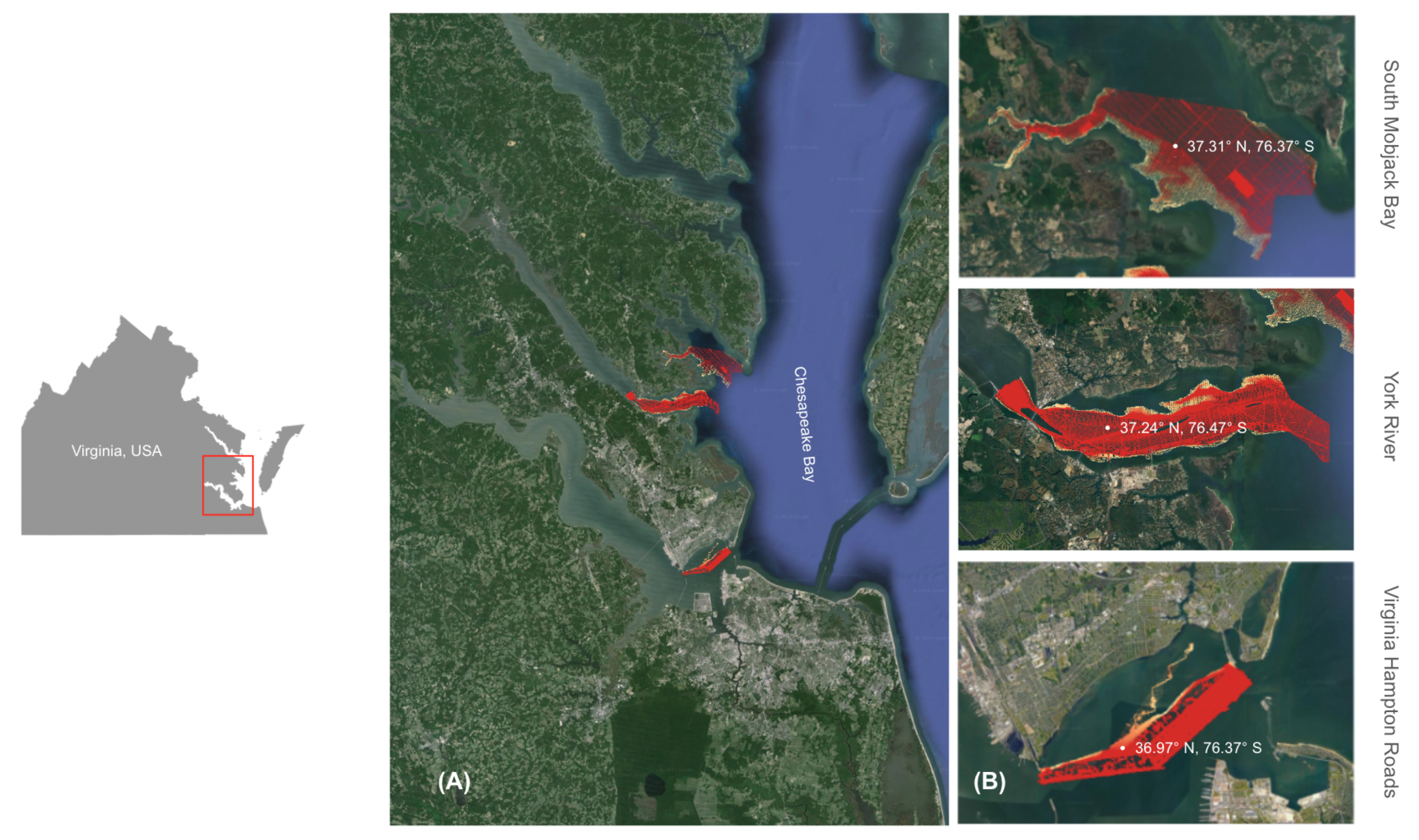
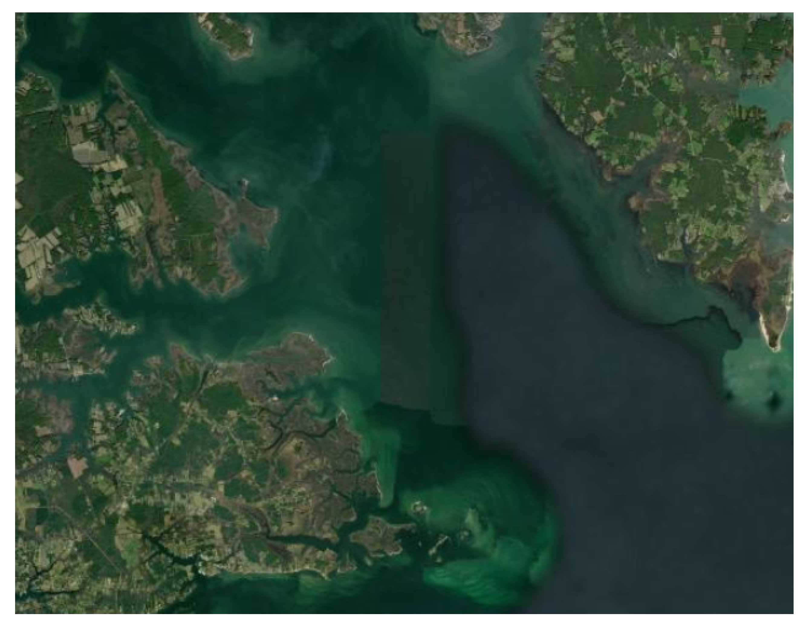
2.1. Study Area

In this study, we focus on 17,239 km of shoreline located in the Commonwealth of Virginia, USA, explicitly seeking to model areas of 5 m depth or shallower which border this region (see Figure 1). The majority of this shoreline surrounds the Chesapeake Bay, a protected estuary responsible for over a hundred billion US dollars of economic output every year, predominantly related to commercial fishing, tourism, recreation, and timber [59]. The Chesapeake Bay is a focus of estuary protection and renewal activities by the Commonwealth of Virginia, and also many US federal agencies [59]. The salinity structure and chemical characteristics of the water here are extremely dynamic, resulting in high levels of turbidity across most of the region [60]. Our study area is defined as regions that have approximately 5 m or shallower depth, as measured by the Continuously Updated DEM (CUDEM); this resulted in a buffer region of approximately 1 km from the shore [61]. The model’s performance was evaluated across three locations: two within the Southern Chesapeake Bay, and a third situated on the western shore of Chesapeake Bay (South Mobjack Bay). Figure 1 shows an overview map of the study area (Figure 1a) and RGB orthophoto maps of the three regions.

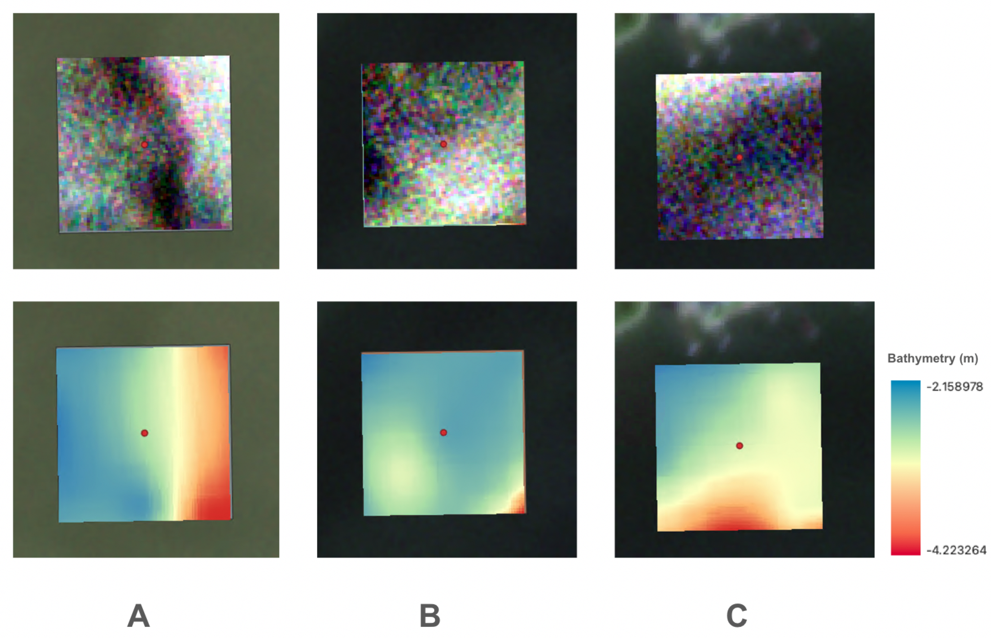
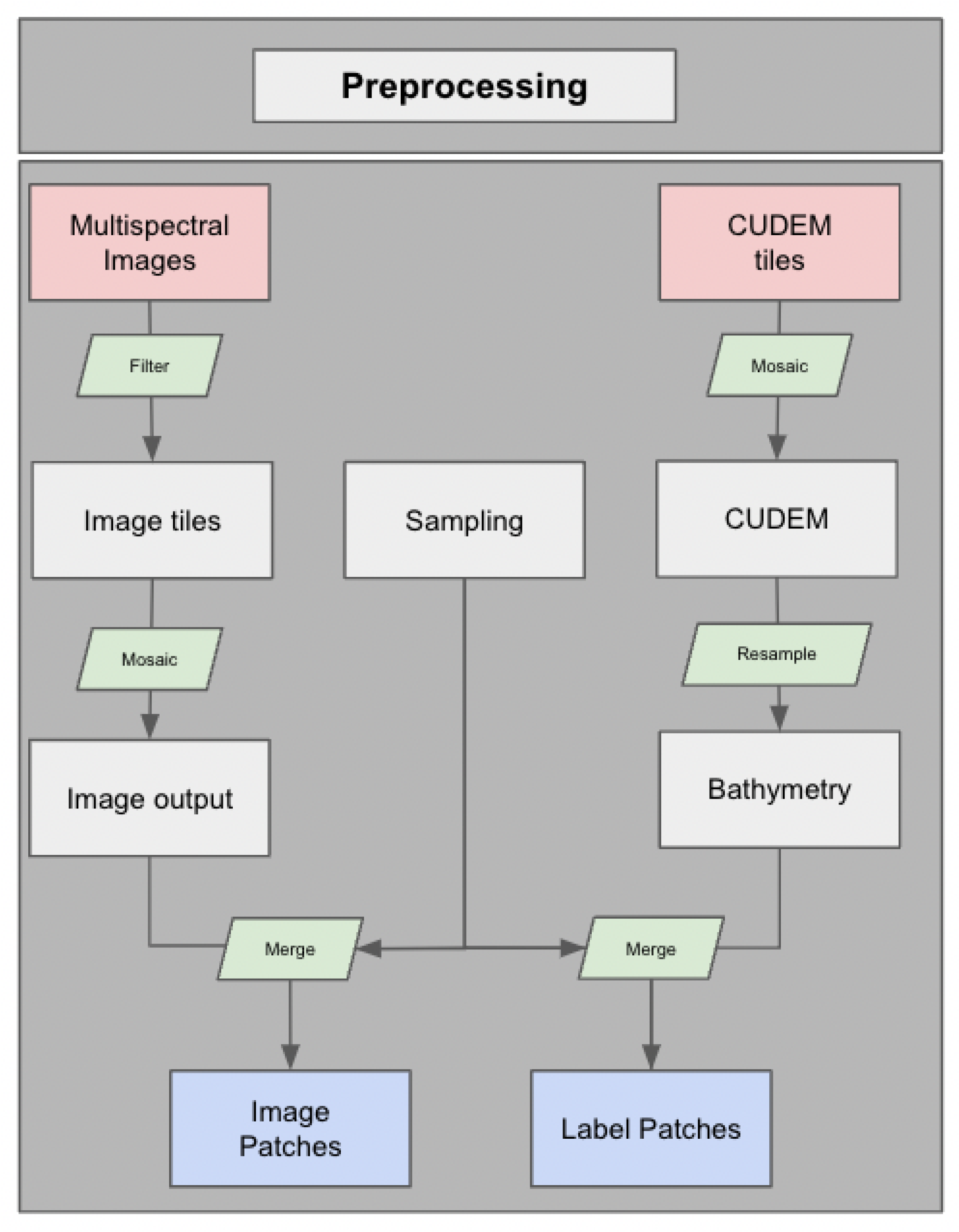
2.2. Data and Preprocessing

2.2.1. High-Resolution Satellite Imagery

Our analysis utilized globally available 8-band, multispectral (Coastal Blue, Blue, Green I, Green, Yellow, Red, RedEdge, NIR), high-resolution satellite images from Planet Labs [63], with a spatial resolution of approximately 3 m (

Table 1. Planet Scope Imagery Wavelength.

Spectral Bands	Wave Length (nm)
Coastal Blue	431–452
Blue	465–515
Green I	513–549
Green	547–583
Yellow	600–620
Red	650–680
RedEdge	697–713
NIR	845–885

summarizes the wavelength range of each band). These bands underwent orthorectification, as well as radiometric, geometric, and atmospheric corrections, resulting in surface reflectance values. Images were manually assessed for inclusion into the study, with each image selected meeting both of the following criteria: (a) zero-cloud conditions during low tide periods to minimize tidal influence, and (b) captured in 2020, the time period closest to the date our evaluation data were collected. A total of eight image tiles, captured throughout the fall of 2020, were carefully selected for further processing. These image tiles were mosaicked into one image with overlapping areas calculated by the mean value of the overlapped pixels.

2.2.2. CUDEM—Bathymetry

The Continuously Updated DEM (CUDEM) Program, developed by NOAA National Centers for Environmental Information (NCEI), provides bare-Earth, topographic–bathymetric, and bathymetric DEMs for the entire coastal United States [19]. The CUDEMs are currently the highest-resolution, seamless depiction of the entire U.S. Atlantic and Gulf Coasts in the public domain; the data provides approximately 3 m coastal topographic–bathymetric DEMs and 10 m offshore bathymetric DEMs. The CUDEM dataset for the Chesapeake Bay area underwent its last update in 2019. Tiles encompassing the study area were retrieved, amalgamated into a mosaic, and subsequently resampled to a 3 m resolution. Similar to the aforementioned process of generating imagery patches, corresponding labeling patches using the CUDEM image were created for each sample. Figure 2 illustrates the CUDEM bathymetry distribution of the sampled data center.

2.2.3. Hydrographic Survey Data

The validation data are sourced from hydrographic surveys conducted and maintained by the National Centers for Environmental Information (NCEI). These surveys employ hydrographic vessels equipped with both multibeam sonar and towed side-scan sonar systems to map the seabed. For validation purposes, three locations in Virginia were selected: two within the Southern Chesapeake Bay-Virginia Hampton Roads and York River, each surveyed in the fall of 2019 and 2020, respectively, and a third situated in South Mobjack Bay, surveyed in the fall of 2020. The bathymetry data grids were Mean Lower Low Water (MLLW) datum; to be consistent with the training data source, each bathymetry data grid was calibrated into the vertical datum NAD83 using NOAA’s Vertical Datum Transformation (VDatum) tool [64].

2.2.4. Sampling Strategy

Training data were collected from a region approximately 1 km from the shoreline. Samples were randomly distributed within this region, ensuring a minimum distance of 200 m between each sample to prevent overlap. This process yielded a total of 4727 sample points with water depths below 5 m for training purposes. For each sample point, a $64\times 64$ pixel, corresponding to a $192\times 192$ meter area patch, was extracted with the sample points at its center.

Today, there is considerable uncertainty regarding optimal patch sizes for different applications, with values from 16 × 16 to 128 × 128 being common [26,28,32,65,66]. The selected tile size of $64\times 64$ pixels provides a balance between capturing detailed bathymetric features and incorporating broader spatial context. Each tile covers an area of approximately $192\times 192$ meters, enabling the model to effectively learn both fine-scale bathymetric characteristics and larger-scale spatial patterns. This balanced spatial coverage is essential for accurately modeling depth variations, particularly in dynamic coastal and marine environments where local details and regional context can jointly influence bathymetric predictions (see Figure 3).

Figure 4 summarizes the entire data preprocessing workflow.

2.3. Methodology

In this section, we describe the methods employed for bathymetric depth estimation. We explore several deep learning approaches, along with a baseline Random Forest method for comparison. Additionally, we outline our evaluation strategy. Each of these techniques is presented in detail below.

2.3.1. Random Forest

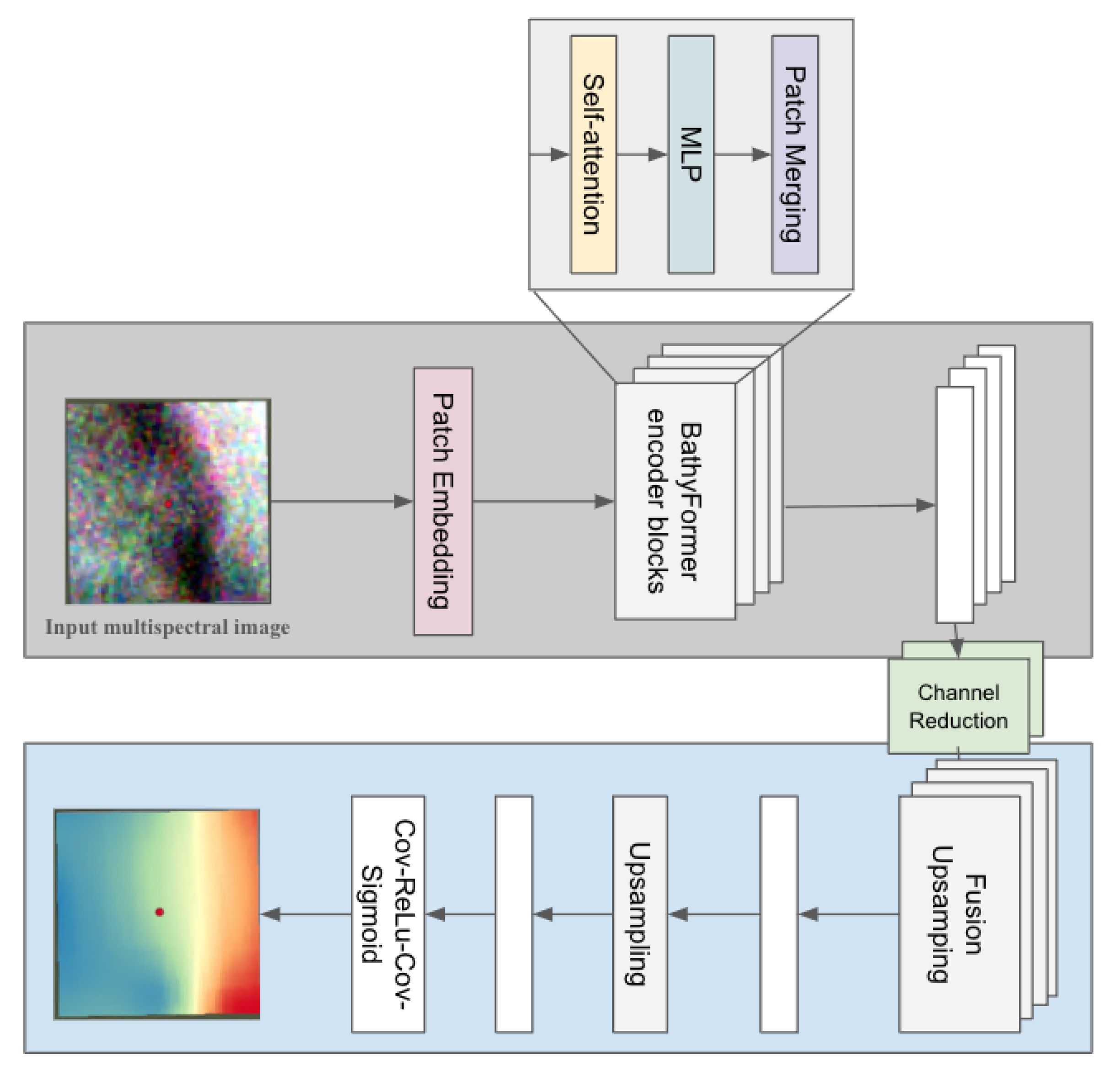
Random Forest (RF), an ensemble learning algorithm introduced in 2001 [67], has become a prominent machine learning technique in remote sensing. The RF algorithm operates by constructing multiple decision trees during training, each trained on a random subset of both the data and the features, and aggregates their outputs for regression or classification predictions [67]. RF’s strength lies in its capacity to handle high-dimensional data and capture complex, nonlinear relationships within multispectral remote sensing data [68,69,70]. By combining the outputs of numerous uncorrelated and independent decision tree models, RF exhibits robust performance and mitigates overfitting, making it well suited for analyzing large-scale remote sensing datasets.

For the estimation of bathymetry from multispectral imagery, all eight available spectral bands were utilized in the model training process. The Random Forest is then trained using a max depth of 10, minimum split size of 2, and 200 component trees (with each value selected through a grid search optimization).

2.3.2. BathyFormer

Transformer-based architectures, initially introduced for natural language processing (NLP), leverage a self-attention mechanism along with multilayer perceptrons (MLP) to address the constraints posed by recurrent neural networks (RNNs) [37]. Since its emergence, the transformer architecture has garnered significant interest across domains, including in computer vision, where a variant known as the vision transformer (ViT) was developed in [36].

In this study, we built on the transformer encoder structure outlined in [71], while drawing inspiration for the decoder component from the hierarchical transformer encoder-decoder framework proposed for monocular depth estimation by [72]. Figure 5 shows a summary of the presented model architecture.

Different from image segmentation, which aims to classify each image pixel with a certain category, the goal of this framework is to predict a continuous pixel-wise map with values representing the depth, $\widehat{Y}\in {\mathbb{R}}^{H\times W\times 1}$, from a given 8-band image, $I\in {\mathbb{R}}^{H\times W\times 8}$ of size H(eight) and W(idth). The encoder, adopted from SegFormer [71], allows a larger effective receptive field than convolutional encoders. The process begins with embedding the $64\times 64\times 8$ input image as a sequence of patches using a $3\times 3$ convolution operation. These embedded patches are then fed into a transformer block consisting of multiple sets of self-attention mechanisms and multilayer perceptron (MLP) layers. Lastly, the resulting output undergoes patch merging through an overlapped convolution technique. This process generates coarse high-resolution features and fine low-resolution features that can be used by the decoder to map the extracted features into a target depth map of $64\times 64\times 1$ in the original dimension.

The BathyFormer architecture is novel in that it is a modification of the optical depth transformer, via the adjustment to accommodate multispectral satellite image bands. By extension, this is the first time an optical depth-based transformer has been applied to satellite imagery.

2.3.3. Loss Function, Optimization, and Evaluation

In order to calculate the difference between predicted output $\widehat{y}$ and ground truth map y, we use a root mean squared error loss function to evaluate algorithm performance for model described in Section 2.3. The loss function is defined as

$$\mathrm{loss}=\sqrt{{\displaystyle \frac{1}{N}}{\displaystyle \sum _i^n}{(y_i-{\widehat{y}}_i)}^2}$$

(1)

where N is the total number of testing cases, $y_i$ is the ground truth bathymetry value collected by hydrographic survey, and $\widehat{y_i}$ is the predicted bathymetry from the model. During the training process for BathyFormer, an Adam optimizer is used to minimize the RMSE loss based on its adaptive learning rate capabilities and efficient handling of sparse gradients. The Adam optimizer was chosen for testing due to its general suitability for a wide range of different applications [26,29,73], as well as it having previously been found successful in a paper seeking to apply transformer-based model architectures in cases of optical depth [72]. Optimizer hyperparameters (learning rate, betas) were searched across using a random search to identify optimal values. We used an initial learning rate of 1 × 10^$-3$ to train the model [74].

We implement a wide range of validation metrics to assess pixel-level prediction and mapping performance. We evaluate the model performance by presenting mean absolute error (MAE), root mean square error (RMSE), and mean absolute percentage error (MAPE), tested with the ground truth data collected by hydrographic survey data.

3. Results

This section presents the results of the BathyFormer depth mapping approach, evaluated using hydrographic survey data from the three locations described in Section 2.2. Figure 6 presents the prediction results for each location. The error distribution relative to the ground truth bathymetry survey data is depicted in Figure 7, while Figure 8 shows the MAPE distribution against the ground truth bathymetry survey data.

Table 2. Error analysis of the prediction results at the three locations with BathyFormer. L1, L2, and L3 represent the location of South Mobjack Bay, York River, and Virginia Hampton Roads, respectively. Each location is presented with three statistics, in meters: MAE (mean absolute error), RMSE (root mean square error), and MAPE (mean absolute percentage error). N represents the number of points in the testing case.

Model	Location	MAE (m)	RMSE (m)	MAPE (%)	N
BathyFormer	L1	0.46	0.55	12.5	271
	L2	0.55	0.69	13.2	1139
	L3	0.55	0.73	11.3	222

and

Table 3. Error analysis of the prediction results at the three locations with Random Forest. L1, L2, and L3 represent the location of South Mobjack Bay, York River, and Virginia Hampton Roads, respectively. Each location is presented with three statistics, in meters: MAE (mean absolute error), RMSE (root mean square error), and MAPE (mean absolute percentage error). N represents the number of points in the testing case.

Model	Location	MAE (m)	RMSE (m)	MAPE (%)	N
Random Forest	L1	0.83	0.97	19.6	271
	L2	1.08	1.24	25.4	1139
	L3	1.13	1.31	25.5	222

summarize the error metrics for each location, tested with an independent testing set using BathyFormer and Random Forest (RF), respectively. When employing BathyFormer, the RMSE values were 0.55 m, 0.69 m, and 0.73 m for South Mobjack Bay, York River, and Virginia Hampton Roads, respectively. In comparison, the RMSE outputs for RF were 0.97 m, 1.24 m, and 1.31 m for the three tested locations. A detailed analysis of these results is provided in the subsequent sections.

3.1. Comparative Analysis of RF and BathyFormer

The comparison of Random Forest and BathyFormer models for bathymetry prediction across three locations (South Mobjack Bay, York River, and the Virginia Hampton Roads) demonstrates consistent and significant performance improvements with BathyFormer. For the South Mobjack Bay area, BathyFormer reduces the MAE by 44.6% (from 0.83 m to 0.46 m), RMSE by 43.3% (from 0.97 m to 0.55 m), and MAPE by 36.2% (from 19.6% to 12.5%) compared with Random Forest. In the York River, BathyFormer achieves even more substantial improvements, reducing MAE by 49.1% (from 1.08 m to 0.55 m), RMSE by 44.4% (from 1.24 m to 0.69 m), and MAPE by 48.0% (from 25.4% to 13.2%). For the areas in the Virginia Hampton Roads, BathyFormer maintains its performance, decreasing MAE by 51.3% (from 1.13 m to 0.55 m), RMSE by 44.3% (from 1.31 m to 0.73 m), and MAPE by 55.7% (from 25.5% to 11.3%).

These results suggest that BathyFormer’s architecture, likely leveraging its ability to capture complex spatial relationships through self-attention mechanisms, is more effective in modeling the bathymetric features of coastal areas. The consistent improvement across different error metrics indicates that BathyFormer not only reduces overall prediction errors but also enhances the model’s performance across various aspects of depth estimation. Notably, BathyFormer’s performance remains robust across all three locations, with MAE consistently around 0.55 m, suggesting good generalization capabilities compared with RF.

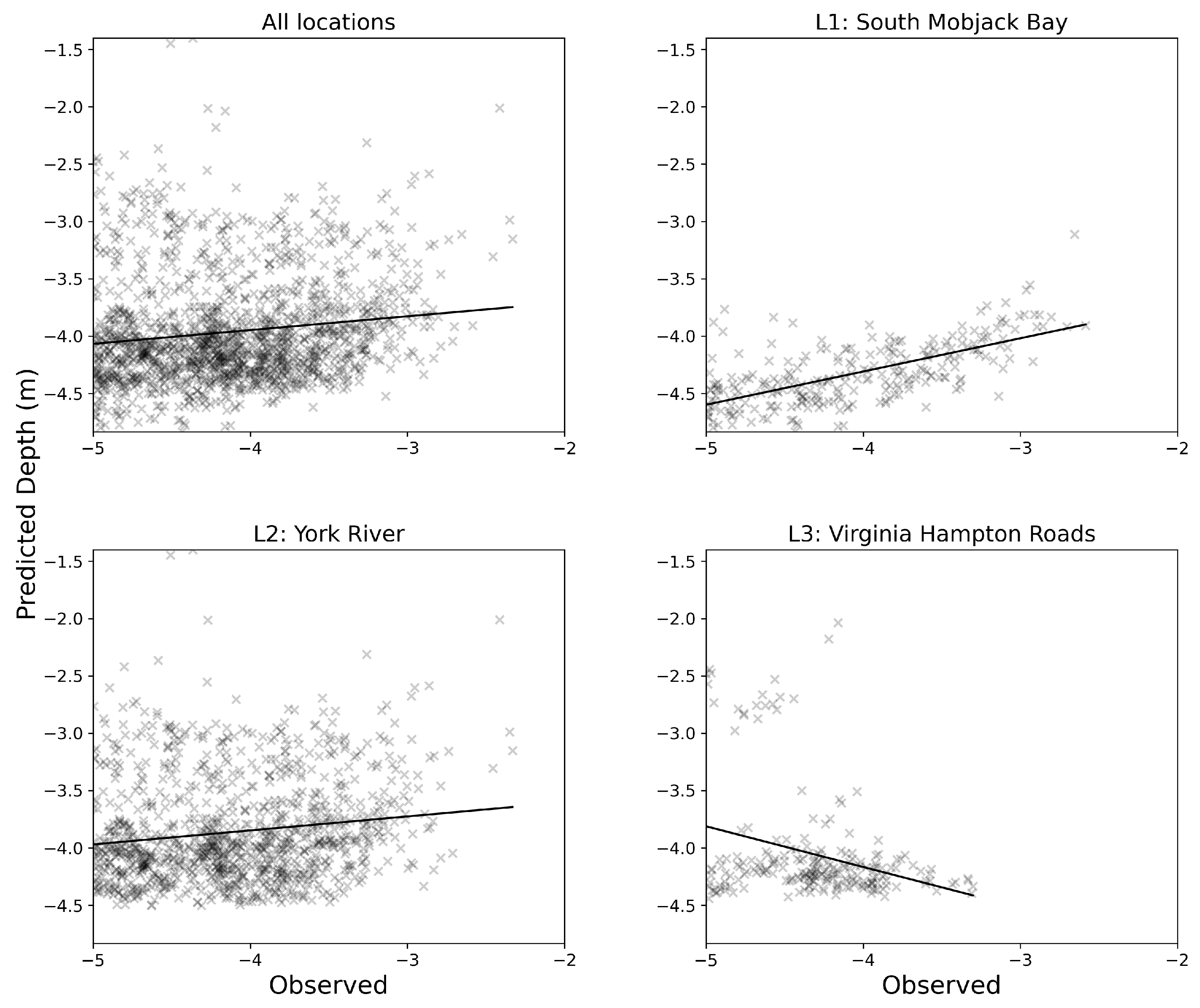
3.2. Comparison of Prediction with Hydrographic Survey

To compare the performance of the SDB model across the three testing areas, a quantitative evaluation was conducted on the model using statistical analyses. For objective testing, all three testing locations are independent of each other and of the training location. Significant variances were observed among the three areas: South Mobjack Bay exhibited the highest estimation accuracy (L1 in the table with RMSE 0.55m and MAPE 12.5%), followed by York River (L2 in the table with RMSE 0.69m and MAPE 13.2%) and Virginia Hampton Roads (with RMSE 0.73m and MAPE 11.3%).

A scatter plot (Figure 6) was generated to visually compare the hydrographic surveyed data and estimated depths across the three testing areas, indicating the strength of fit between the BathyFormer-derived estimates (y axis) and a hydrographic survey (x axis) for the validation dataset. A plot closer to the 1:1 line (dotted in black) indicated that the model better represented the real values. Among the three locations tested, the estimated depths in the Hampton Roads region are predominantly clustered within the 3.8 to 4.4 m depth range, irrespective of the variations in actual depth. Meanwhile, higher accuracy was achieved at depths of 3 to 5 m in South Mobjack Bay and York River.

Figure 7 shows the relationship between absolute error and surveyed depth for each of the three locations and aggregated set, in which each point on the figure is a single testing point. For the aggregated sets, there was no strong correlation between increasing the observed depths and the error in the estimate from the satellite imagery. However, in the Southern Chesapeake Bay area (York River and Virginia Hampton Roads shown as L2 and L3 in Figure 7), the prediction errors tend to decrease in shallow water regions, while the prediction errors in the western shore of Chesapeake Bay (South Mobjack Bay) tend to increase with the decrease in water depth.

To understand the average magnitude of error produced by the model at different depths, Figure 8 displays the relationship between the MAPE error and surveyed depth for each of the three locations and the aggregated set. This figure illustrates how the percentage of error changes with varying water depths. The MAPE values range from 11.3% to 13.2% across the three tested locations, indicating that the average absolute percentage difference between the predictions and the surveyed data lies within this range. Notably, errors tend to be higher at greater depths in Southern Chesapeake Bay, while the opposite pattern is observed on the western shore of Chesapeake Bay.

To understand the model prediction error distribution over different depths,

Table 4. Error analysis of the prediction results at different depths ranging from 2 m to 5 m. Each depth error analysis is presented with three statistics, MAE (mean absolute error), RMSE (root mean square error), and MAPE (mean absolute percentage error).

Error Metrics	2–3 (m)	3–4 (m)	4–5 (m)
MAE (%)	0.82	0.46	0.56
RMSE (m)	0.89	0.52	0.75
MAPE (%)	29	12.9	12

summarizes the error results for the depth. The bathymetry prediction model exhibited varying performance across different depth ranges. In the shallow water zone (2–3 m), the model demonstrated the highest error rates with an MAE of 0.82 m, RMSE of 0.89 m, and MAPE of 29%. The mid-range depths (3–4 m) showed markedly improved accuracy, with the lowest MAE of 0.46 m, RMSE of 0.52 m, and a substantially reduced MAPE of 12.9%. For the deeper range (4–5 m), the model maintained relatively good performance with a slight increase in absolute errors (MAE of 0.56 m, RMSE of 0.75 m) compared with the mid-range, while the MAPE further decreased to 12%, indicating the best relative accuracy among all depth ranges. These results suggest a nonlinear relationship between prediction accuracy and water depth, with the model performing optimally in a water depth of over 3 m.

4. Discussion

The results from this study demonstrate that optical imagery, when combined with convolutional neural networks and transformers, can estimate nearshore depth with an average accuracy of between 86.8 and 88.7% (MAPE). While this finding is notable, it is mediated by a number of different factors. In this section, we discuss our findings and the factors that may have affected them.

4.1. Impact of Water Turbidity and Seabed Sediments

One significant source of error in our approach is likely due to the turbidity of the target areas. In water bodies that are significantly affected by tides and predominantly covered by sediment in the nearshore (such as the South Mabjack Bay on the western shore of the Chesapeake Bay (see Figure 9)), seabed fine-grained sediments are frequently resuspended due to strong and recurring tidal currents. This resuspension causes an increase in water turbidity (i.e., cloudiness) [60]. Water bodies such as the southern end of the Chesapeake Bay are also significantly affected by seasonal and spatial variations in surface water turbidity [60]. The strong and recurring tidal currents near the entrance of the South Bay result in a large amount of suspended sediment, thereby increasing turbidity levels in these areas [60]. Variations in turbidity could contribute to uncertainty in model estimates [75,76].

Suspended sediment also exhibits seasonal variations, with higher turbidity during the winter season (October through March), initiated by a fall diatom bloom and maintained by extended periods of high wind [60,77]. Satellite imagery was collected from September to December 2020, coinciding with the timing of the hydrographic surveys. Consequently, the prediction errors may also be influenced by seasonal water turbidity.

We see some evidence of this in our results. In regions with high turbidity, shallow water depths are overestimated, while deeper depths are underestimated, leading to poor mapping performance. This discrepancy is particularly notable in Virginia’s Hampton Roads, as shown in Figure 6.

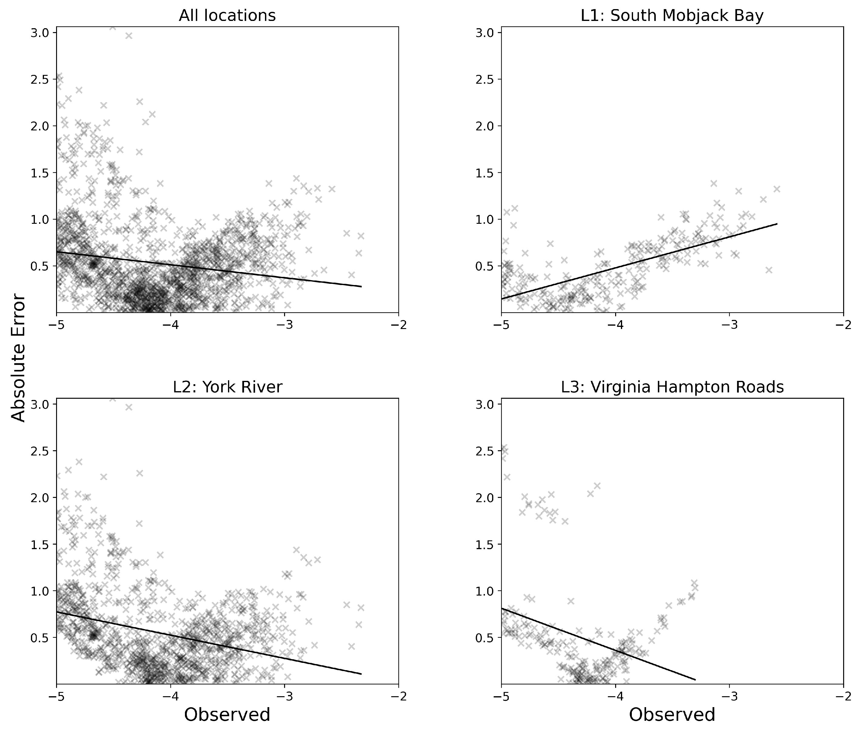
4.2. Accuracy Discrepancy Among Different Water Depths

The bathymetry prediction model demonstrates varying performance across different depth ranges, revealing complex patterns in its accuracy. The model achieves its best performance in the mid-depth range (3–4 m), with the lowest MAE (0.46%) and RMSE (0.52 m), suggesting an optimal zone where factors like light penetration and bottom reflectance may be ideally balanced. However, shallow waters (2–3 m) present significant challenges, evidenced by higher error rates across all metrics, likely due to complex nearshore processes and variable bottom reflectance. Interestingly, while absolute errors (MAE and RMSE) slightly increase in deeper waters (4–5 m) compared with the mid-range, the relative accuracy improves, as indicated by the lower MAPE (12%). This suggests that the model’s predictions become more stable and relatively accurate as depth increases, despite a slight decrease in absolute accuracy. The transition from high relative errors in shallow waters to lower relative errors in deeper waters implies that the model might be overestimating depth variability in shallow areas. These performance variations across depths have important implications for the model’s architecture and application. It suggests that a single model might not be optimal for all depth ranges, and depth-specific models or ensemble methods could be considered for future exploration.

4.3. Data Limitations in Shallow Water

The validation data were obtained through hydrographic surveys conducted at three independent locations: South Mobjack Bay, York River, and Hampton Roads, Virginia. South Mobjack Bay is situated on the western shore of the Chesapeake Bay, while the other two sites are located within the southern Chesapeake Bay. These data were collected from vessel-based surveys along the coast, primarily targeting areas deeper than 2 m in depth with the maximum allowable uncertainties between 0.5 and 0.6 m, as accessing shallower waters less than 2 m posed safety issues for vessels. Consequently, our validation results are less reliable for depths less than 2 m.

To explore this limitation and further validate the predictions in shallow waters of less than 2 m, we randomly selected 484 location points within the three study areas, ensuring these points are independent of the training data. The depth values for these sample points were extracted from the CUDEM dataset, serving as an alternative source of ground truth for validation. The root mean square error (RMSE) for these sample points, ranging from 0 to 2 m in depth, is 1.14 m.

While this validation is flawed in many ways—i.e., the CUDEM is relatively coarse resolution and not created at a time or scale that matches our imagery—it does suggest that more work remains to be carried out on extremely nearshore (2 m depth and less) estimates. We have made modest improvements by further fine-tuning the model with only data sampled from depths less than 2 m, achieving up to a 0.45 RMSE in regions having bathymetry depths less than 2 m. However, significant work remains to be conducted.

Figure 10 shows a comparison of estimated results at bathymetry depths less than 2 m. The results shallower than 2 m depth show a similar prediction pattern compared with regions above 2 m (see Figure 6), where the model tends to underestimate in areas from 1 to 2 m depth, and overestimate in areas less than 1 m depth. The corresponding absolute error distribution in Figure 11 also shows the same pattern compared with regions deeper than 2 m, with prediction errors decreasing with decreasing water depth.

Fine-tuning the model with data from depths below 2 m significantly reduces the error of such areas by 60%, decreasing the RMSE from 1.14 m to 0.45 m. However, the study did not produce a model that can be scaled to predict all nearshore water depths due to limitations such as data availability, turbidity, and other factors. For future studies, a model suitable for all nearshore depths prediction could be more helpful for rapid nearshore bathymetry mapping.

4.4. Limitations Caused Due to Discrepancies Between Labeled and Ground Truth Bathymetry

Accurate labeling is essential for training the pixel-wise vision transformer model. In this study, we utilized CUDEM data as the continuous ground truth bathymetry source to label the multispectral imagery, operating under the assumption that CUDEM accurately reflects real bathymetric data. This dataset is the result of combining and interpolating multiple data sources, including hydrographic surveys, multibeam sonar, the USGS National Map, digitized bathymetric charts, topographic maps, shorelines, satellite-derived elevation, and U.S. Army Corps of Engineers (USACE) Navigation Condition Surveys [19]. The interpolation methods used to generate the final dataset are varied, resulting in an estimated interpolation that may not accurately represent ground truth bathymetric data in areas distant from the source points. These limitations of the labeling data introduce several constraints and future directions. Since the labeling of the CUDEM data may not directly reflect actual depth, during model training, proper correlation between the multispectral imagery and depth values may be hampered. Further testing with concurrently collected bathymetric data and multispectral imagery could help test this hypothesis.

4.5. Future Directions

The future direction of satellite-derived bathymetry research is poised to harness advancements in remote sensing technologies and artificial intelligence to improve accuracy and expand applicability. Various image filtering and preprocessing strategies could potentially enhance the accuracy of final model predictions. The current study does not account for the effects of sun glint, which is caused by the specular reflection of sunlight on the water’s surface. Sun glint can potentially saturate the sensor, leading to distortions in bathymetry predictions. Improving the imagery preprocessing strategy to automatically or statistically remove the effects of sun glint could significantly enhance the accuracy of the prediction results by eliminating this source of distortion [78,79]. These enhancements could include using images captured at the same time of day when creating mosaics from different locations and excluding images taken during algae bloom seasons. Additionally, different patch sizes could also impact the results found in this work. Another promising approach is the integration of data from multiple sources, such as LiDAR and sonar, which provide detailed information about water depth and seabed characteristics. This integrated approach will allow for a more comprehensive understanding of underwater topography, facilitating a wide range of applications.

5. Conclusions

The work presented in this paper provides two contributions to the literature. First, this paper demonstrates the first application of a transformer-based model for bathymetry prediction from multispectral satellite imagery. Second, the BathyFormer model was trained with high-resolution multispectral imagery to predict nearshore shallow water bathymetry, achieving RMSE values ranging from 0.55 to 0.73 m at different testing locations for water depths between 2 and 5 m. When the model was refined with data collected at depths shallower than 2 m, an RMSE value of 0.45 m was achieved for these areas.

This paper shows that optical imagery can be a useful tool for mapping bathymetry, especially in the context of transformer-based models. However, a number of future directions remain. First, incorporating hyperspectral data can improve depth estimation accuracy. These data types provide more detailed information about water and seabed characteristics, which can enhance model performance, particularly in environments heavily influenced by turbidity and sediment. Second, concurrent data collection of bathymetry and high-resolution remotely sensed data can minimize discrepancies between training data and corresponding labels caused by temporal changes in the underwater environment, such as sediment transport, tidal variations, and seasonal changes. With advancements in computational power and efficient transformer architectures, real-time or near-real-time bathymetry mapping from satellite imagery will become feasible. This is particularly useful for monitoring coastal changes, supporting disaster response, and informing navigation safety. Third, future research can explore the fusion of satellite imagery with other data sources, such as LiDAR, sonar, and UAV. This approach may enhance model performance, as transformers can effectively integrate these heterogeneous data types, resulting in more comprehensive and accurate bathymetric models.

References

1. Nunez, K.; Rudnicky, T.; Mason, P.; Tombleson, C.; Berman, M. A geospatial modeling approach to assess site suitability of living shorelines and emphasize best shoreline management practices. Ecol. Eng. 2022, 179, 106617. [Google Scholar] [CrossRef]
2. Twomey, A.J.; Nunez, K.; Carr, J.A.; Crooks, S.; Friess, D.A.; Glamore, W.; Orr, M.; Reef, R.; Rogers, K.; Waltham, N.J.; et al. Planning hydrological restoration of coastal wetlands: Key model considerations and solutions. Sci. Total Environ. 2024, 915, 169881. [Google Scholar] [CrossRef]
3. Ye, F.; Zhang, Y.J.; Wang, H.V.; Friedrichs, M.A.; Irby, I.D.; Alteljevich, E.; Valle-Levinson, A.; Wang, Z.; Huang, H.; Shen, J.; et al. A 3D unstructured-grid model for Chesapeake Bay: Importance of bathymetry. Ocean Model. 2018, 127, 16–39. [Google Scholar] [CrossRef]
4. Cai, X.; Zhang, Y.J.; Shen, J.; Wang, H.; Wang, Z.; Qin, Q.; Ye, F. A Numerical Study of Hypoxia in Chesapeake Bay Using an Unstructured Grid Model: Validation and Sensitivity to Bathymetry Representation. JAWRA J. Am. Water Resour. Assoc. 2022, 58, 898–921. [Google Scholar] [CrossRef]
5. Du, J.; Shen, J.; Zhang, Y.J.; Ye, F.; Liu, Z.; Wang, Z.; Wang, Y.P.; Yu, X.; Sisson, M.; Wang, H.V. Tidal Response to Sea-Level Rise in Different Types of Estuaries: The Importance of Length, Bathymetry, and Geometry. Geophys. Res. Lett. 2018, 45, 227–235. [Google Scholar] [CrossRef]
6. Ashphaq, M.; Srivastava, P.K.; Mitra, D. Review of near-shore satellite derived bathymetry: Classification and account of five decades of coastal bathymetry research. J. Ocean Eng. Sci. 2021, 6, 340–359. [Google Scholar] [CrossRef]
7. Gao, J. Bathymetric mapping by means of remote sensing: Methods, accuracy and limitations. Prog. Phys. Geogr. Earth Environ. 2009, 33, 103–116. [Google Scholar] [CrossRef]
8. Najar, M.A.; Benshila, R.; Bennioui, Y.E.; Thoumyre, G.; Almar, R.; Bergsma, E.W.J.; Delvit, J.M.; Wilson, D.G. Coastal Bathymetry Estimation from Sentinel-2 Satellite Imagery: Comparing Deep Learning and Physics-Based Approaches. Remote Sens. 2022, 14, 1196. [Google Scholar] [CrossRef]
9. Mateo-Pérez, V.; Corral-Bobadilla, M.; Ortega-Fernández, F.; Vergara-González, E.P. Port Bathymetry Mapping Using Support Vector Machine Technique and Sentinel-2 Satellite Imagery. Remote Sens. 2020, 12, 69. [Google Scholar] [CrossRef]
10. Caballero, I.; Stumpf, R.P. Retrieval of nearshore bathymetry from Sentinel-2A and 2B satellites in South Florida coastal waters. Estuar. Coast. Shelf Sci. 2019, 226, 106277. [Google Scholar] [CrossRef]
11. Sagawa, T.; Yamashita, Y.; Okumura, T.; Yamanokuchi, T. Satellite Derived Bathymetry Using Machine Learning and Multi-Temporal Satellite Images. Remote Sens. 2019, 11, 1155. [Google Scholar] [CrossRef]
12. Turner, I.L.; Harley, M.D.; Almar, R.; Bergsma, E.W.J. Satellite optical imagery in Coastal Engineering. Coast. Eng. 2021, 167, 103919. [Google Scholar] [CrossRef]
13. Caballero, I.; Stumpf, R.P. Confronting turbidity, the major challenge for satellite-derived coastal bathymetry. Sci. Total Environ. 2023, 870, 161898. [Google Scholar] [CrossRef]
14. Lyzenga, D.R. Remote sensing of bottom reflectance and water attenuation parameters in shallow water using aircraft and Landsat data. Int. J. Remote Sens. 1981, 2, 71–82. [Google Scholar] [CrossRef]
15. Caballero, I.; Stumpf, R.P. Towards Routine Mapping of Shallow Bathymetry in Environments with Variable Turbidity: Contribution of Sentinel-2A/B Satellites Mission. Remote Sens. 2020, 12, 451. [Google Scholar] [CrossRef]
16. Poppenga, S.K.; Palaseanu-Lovejoy, M.; Gesch, D.B.; Danielson, J.J.; Tyler, D.J. Evaluating the Potential for Near-Shore Bathymetry on the Majuro Atoll, Republic of the Marshall Islands, Using Landsat 8 and WorldView-3 Imagery; U.S. Geological Survey: Reston, VA, USA, 2018. [Google Scholar] [CrossRef]
17. Mandlburger, G.; Kölle, M.; Nübel, H.; Soergel, U. BathyNet: A Deep Neural Network for Water Depth Mapping from Multispectral Aerial Images. PFG J. Photogramm. 2021, 89, 71–89. [Google Scholar] [CrossRef]
18. Yustisi Lumban-Gaol, K.A.O.; Peters, R. Extracting Coastal Water Depths from Multi-Temporal Sentinel-2 Images Using Convolutional Neural Networks. Mar. Geod. 2022, 45, 615–644. [Google Scholar] [CrossRef]
19. Amante, C.J.; Love, M.; Carignan, K.; Sutherland, M.G.; MacFerrin, M.; Lim, E. Continuously Updated Digital Elevation Models (CUDEMs) to Support Coastal Inundation Modeling. Remote Sens. 2023, 15, 1702. [Google Scholar] [CrossRef]
20. Zhong, J.; Sun, J.; Lai, Z.; Song, Y. Nearshore Bathymetry from ICESat-2 LiDAR and Sentinel-2 Imagery Datasets Using Deep Learning Approach. Remote Sens. 2022, 14, 4229. [Google Scholar] [CrossRef]
21. Guo, X.; Jin, X.; Jin, S. Shallow Water Bathymetry Mapping from ICESat-2 and Sentinel-2 Based on BP Neural Network Model. Water 2022, 14, 3862. [Google Scholar] [CrossRef]
22. Hsu, H.J.; Huang, C.Y.; Jasinski, M.; Li, Y.; Gao, H.; Yamanokuchi, T.; Wang, C.G.; Chang, T.M.; Ren, H.; Kuo, C.Y.; et al. A semi-empirical scheme for bathymetric mapping in shallow water by ICESat-2 and Sentinel-2: A case study in the South China Sea. ISPRS J. Photogramm. Remote Sens. 2021, 178, 1–19. [Google Scholar] [CrossRef]
23. Albright, A.; Glennie, C. Nearshore Bathymetry From Fusion of Sentinel-2 and ICESat-2 Observations. IEEE Geosci. Remote Sens. Lett. 2021, 18, 900–904. [Google Scholar] [CrossRef]
24. Perbet, P.; Guindon, L.; Côté, J.F.; Béland, M. Evaluating deep learning methods applied to Landsat time series subsequences to detect and classify boreal forest disturbances events: The challenge of partial and progressive disturbances. Remote Sens. Environ. 2024, 306, 114107. [Google Scholar] [CrossRef]
25. Brewer, E.; Lin, J.; Kemper, P.; Hennin, J.; Runfola, D. Predicting road quality using high resolution satellite imagery: A transfer learning approach. PLoS ONE 2021, 16, e253370. [Google Scholar] [CrossRef]
26. Lv, Z.; Nunez, K.; Brewer, E.; Runfola, D. Mapping the tidal marshes of coastal Virginia: A hierarchical transfer learning approach. GIScience Remote Sens. 2024, 61, 2287291. [Google Scholar] [CrossRef]
27. Fayad, I.; Ciais, P.; Schwartz, M.; Wigneron, J.P.; Baghdadi, N.; de Truchis, A.; d’Aspremont, A.; Frappart, F.; Saatchi, S.; Sean, E.; et al. Hy-TeC: A hybrid vision transformer model for high-resolution and large-scale mapping of canopy height. Remote Sens. Environ. 2024, 302, 113945. [Google Scholar] [CrossRef]
28. Tolan, J.; Yang, H.I.; Nosarzewski, B.; Couairon, G.; Vo, H.V.; Brandt, J.; Spore, J.; Majumdar, S.; Haziza, D.; Vamaraju, J.; et al. Very high resolution canopy height maps from RGB imagery using self-supervised vision transformer and convolutional decoder trained on aerial lidar. Remote Sens. Environ. 2024, 300, 113888. [Google Scholar] [CrossRef]
29. Lv, Z.; Nunez, K.; Brewer, E.; Runfola, D. pyShore: A deep learning toolkit for shoreline structure mapping with high-resolution orthographic imagery and convolutional neural networks. Comput. Geosci. 2023, 171, 105296. [Google Scholar] [CrossRef]
30. Runfola, D.; Stefanidis, A.; Lv, Z.; O’Brien, J.; Baier, H. A multi-glimpse deep learning architecture to estimate socioeconomic census metrics in the context of extreme scope variance. Int. J. Geogr. Inf. Sci. 2024, 38, 726–750. [Google Scholar] [CrossRef]
31. Runfola, D.; Stefanidis, A.; Baier, H. Using satellite data and deep learning to estimate educational outcomes in data-sparse environments. Remote. Sens. Lett. 2021, 13, 87–97. [Google Scholar] [CrossRef]
32. Brewer, E.; Valdrighi, G.; Solunke, P.; Rulff, J.; Piadyk, Y.; Lv, Z.; Poco, J.; Silva, C. Granularity at Scale: Estimating Neighborhood Socioeconomic Indicators From High-Resolution Orthographic Imagery and Hybrid Learning. IEEE J. Sel. Top. Appl. Earth Obs. Remote Sens. 2024, 17, 5668–5679. [Google Scholar] [CrossRef]
33. Brewer, E.; Lin, J.; Runfola, D. Susceptibility & defense of satellite image-trained convolutional networks to backdoor attacks. Inf. Sci. 2022, 603, 244–261. [Google Scholar] [CrossRef]
34. Brewer, E.; Lv, Z.; Runfola, D. Tracking the industrial growth of modern China with high-resolution panchromatic imagery: A sequential convolutional approach. arXiv 2024, arXiv:2301.09620. [Google Scholar]
35. Runfola, D.; Baier, H.; Mills, L.; Naughton-Rockwell, M.; Stefanidis, A. Deep Learning Fusion of Satellite and Social Information to Estimate Human Migratory Flows. Trans. GIS 2022, 26, 2495–2518. [Google Scholar] [CrossRef]
36. Dosovitskiy, A.; Beyer, L.; Kolesnikov, A.; Weissenborn, D.; Zhai, X.; Unterthiner, T.; Dehghani, M.; Minderer, M.; Heigold, G.; Gelly, S.; et al. An Image is Worth 16×16 Words: Transformers for Image Recognition at Scale. In Proceedings of the ICLR 2021—9th International Conference on Learning Representations, Virtual Event, Austria, 3–7 May 2021. [Google Scholar]
37. Vaswani, A.; Brain, G.; Shazeer, N.; Parmar, N.; Uszkoreit, J.; Jones, L.; Gomez, A.N.; Kaiser, Ł.; Polosukhin, I. Attention Is All You Need. arXiv 2017, arXiv:1706.03762. [Google Scholar]
38. Ranftl, R.; Bochkovskiy, A.; Koltun, V. Vision Transformers for Dense Prediction. arXiv 2021, arXiv:2103.13413. [Google Scholar]
39. Saeidi, V.; Seydi, S.T.; Kalantar, B.; Shabani, F. Water depth estimation from Sentinel-2 imagery using advanced machine learning methods and explainable artificial intelligence. Geomat. Nat. Hazards Risk 2023, 14, 2225691. [Google Scholar] [CrossRef]
40. Wei, J.; Wang, M.; Lee, Z.; Briceño, H.O.; Yu, X.; Jiang, L.; Garcia, R.; Wang, J.; Luis, K. Shallow water bathymetry with multi-spectral satellite ocean color sensors: Leveraging temporal variation in image data. Remote Sens. Environ. 2020, 250, 112035. [Google Scholar] [CrossRef]
41. Hedley, J.; Roelfsema, C.; Phinn, S.R. Efficient radiative transfer model inversion for remote sensing applications. Remote Sens. Environ. 2009, 113, 2527–2532. [Google Scholar] [CrossRef]
42. Pacheco, A.; Horta, J.; Loureiro, C.; Ferreira, Ó. Retrieval of nearshore bathymetry from Landsat 8 images: A tool for coastal monitoring in shallow waters. Remote Sens. Environ. 2015, 159, 102–116. [Google Scholar] [CrossRef]
43. Hedley, J.D.; Roelfsema, C.; Brando, V.; Giardino, C.; Kutser, T.; Phinn, S.; Mumby, P.J.; Barrilero, O.; Laporte, J.; Koetz, B. Coral reef applications of Sentinel-2: Coverage, characteristics, bathymetry and benthic mapping with comparison to Landsat 8. Remote Sens. Environ. 2018, 216, 598–614. [Google Scholar] [CrossRef]
44. Lyzenga, D.; Malinas, N.; Tanis, F. Multispectral bathymetry using a simple physically based algorithm. IEEE Trans. Geosci. Remote Sens. 2006, 44, 2251–2259. [Google Scholar] [CrossRef]
45. Stumpf, R.P.; Holderied, K.; Sinclair, M. Determination of water depth with high-resolution satellite imagery over variable bottom types. Limnol. Oceanogr. 2003, 48, 547–556. [Google Scholar] [CrossRef]
46. Casal, G.; Monteys, X.; Hedley, J.; Harris, P.; Cahalane, C.; McCarthy, T. Assessment of empirical algorithms for bathymetry extraction using Sentinel-2 data. Int. J. Remote Sens. 2019, 40, 2855–2879. [Google Scholar] [CrossRef]
47. Dörnhöfer, K.; Göritz, A.; Gege, P.; Pflug, B.; Oppelt, N. Water Constituents and Water Depth Retrieval from Sentinel-2A—A First Evaluation in an Oligotrophic Lake. Remote Sens. 2016, 8, 941. [Google Scholar] [CrossRef]
48. Duplančić Leder, T.; Baučić, M.; Leder, N.; Gilić, F. Optical Satellite-Derived Bathymetry: An Overview and WoS and Scopus Bibliometric Analysis. Remote Sens. 2023, 15, 1294. [Google Scholar] [CrossRef]
49. Wu, Z.; Mao, Z.; Shen, W.; Yuan, D.; Zhang, X.; Huang, H. Satellite-derived bathymetry based on machine learning models and an updated quasi-analytical algorithm approach. Opt. Express 2022, 30, 16773–16793. [Google Scholar] [CrossRef]
50. Wicaksono, P.; Harahap, S.D.; Hendriana, R. Satellite-derived bathymetry from WorldView-2 based on linear and machine learning regression in the optically complex shallow water of the coral reef ecosystem of Kemujan island. Remote Sens. Appl. Soc. Environ. 2024, 33, 101085. [Google Scholar] [CrossRef]
51. Mudiyanselage, S.; Abd-Elrahman, A.; Wilkinson, B.; and, V.L. Satellite-derived bathymetry using machine learning and optimal Sentinel-2 imagery in South-West Florida coastal waters. GIScience Remote Sens. 2022, 59, 1143–1158. [Google Scholar] [CrossRef]
52. Ma, Y.; Xu, N.; Liu, Z.; Yang, B.; Yang, F.; Wang, X.H.; Li, S. Satellite-derived bathymetry using the ICESat-2 lidar and Sentinel-2 imagery datasets. Remote Sens. Environ. 2020, 250, 112047. [Google Scholar] [CrossRef]
53. Xie, C.; Chen, P.; Zhang, Z.; Pan, D. Satellite-derived bathymetry combined with Sentinel-2 and ICESat-2 datasets using machine learning. Front. Earth Sci. 2023, 11, 1111817. [Google Scholar] [CrossRef]
54. Casal, G.; Harris, P.; Monteys, X.; Hedley, J.; Cahalane, C.; and, T.M. Understanding satellite-derived bathymetry using Sentinel 2 imagery and spatial prediction models. GIScience Remote Sens. 2020, 57, 271–286. [Google Scholar] [CrossRef]
55. Çelik, O.; Büyüksalih, G.; Gazioğlu, C. Improving the Accuracy of Satellite-Derived Bathymetry Using Multi-Layer Perceptron and Random Forest Regression Methods: A Case Study of Tavşan Island. J. Mar. Sci. Eng. 2023, 11, 2090. [Google Scholar] [CrossRef]
56. Wei, C.; Zhao, Q.; Lu, Y.; Fu, D. Assessment of Empirical Algorithms for Shallow Water Bathymetry Using Multi-Spectral Imagery of Pearl River Delta Coast, China. Remote Sens. 2021, 13, 3123. [Google Scholar] [CrossRef]
57. Najar, M.A.; Thoumyre, G.; Bergsma, E.W.; Almar, R.; Benshila, R.; Wilson, D.G. Satellite derived bathymetry using deep learning. Mach. Learn. 2023, 112, 1107–1130. [Google Scholar]
58. Aleissaee, A.A.; Kumar, A.; Anwer, R.M.; Khan, S.; Cholakkal, H.; Xia, G.S.; Khan, F.S. Transformers in Remote Sensing: A Survey. Remote Sens. 2023, 15, 1860. [Google Scholar] [CrossRef]
59. Phillips, S.; McGee, B. The Economic Benefits of Cleaning Up the Chesapeake; Technical report; Chesapeake Bay Program: Annapolis, MD, USA, 2014. [Google Scholar]
60. Melchor, J.R. Surface Water Turbidity in the Entrance to Chesapeake Bay, Virginia. Master’s Thesis, Old Dominion University, Norfolk, VA, USA, 1972. [Google Scholar] [CrossRef]
61. NOAA. NOAA Continually Updated Shoreline Product (CUSP). 2021. Available online: https://shoreline.noaa.gov/data/datasheets/cusp.html (accessed on 1 January 2024).
62. GLAD. Landsat Analysis Ready Data. 2018. Available online: https://glad.umd.edu/ (accessed on 1 July 2022).
63. PlanetLabs. Planet Application Program Interface: In Space for Life on Earth, 2022.
64. OCS. 2024: Vertical Datum Transformation. 2024. Available online: https://www.fisheries.noaa.gov/inport/item/39987 (accessed on 1 January 2024).
65. Shin, H.C.; Roth, H.R.; Gao, M.; Lu, L.; Xu, Z.; Nogues, I.; Yao, I.; Mollura, D.; Summers, R.M. Deep Convolutional Neural Networks for Computer-Aided Detection: CNN Architectures, Dataset Characteristics and Transfer Learning. IEEE Trans. Med. Imaging 2016, 66, 1285–1298. [Google Scholar] [CrossRef]
66. Zagoruyko, S.; Komodakis, N. Learning to compare image patches via convolutional neural networks. In Proceedings of the 2015 IEEE Conference on Computer Vision and Pattern Recognition (CVPR), Boston, MA, USA, 7–12 June 2015; pp. 4353–4361. [Google Scholar] [CrossRef]
67. Breiman, L. Random Forest. Mach. Learn. 2001, 45, 5–32. [Google Scholar] [CrossRef]
68. Cutler, D.R.; Edwards, T.C., Jr.; Beard, K.H.; Cutler, A.; Gibson, J.; Lawler, J.J. Random Forests for classification in ecology. Ecology 2007, 88, 2783–2792. [Google Scholar] [CrossRef]
69. Sheykhmousa, M.; Mahdianpari, M.; Ghanbari, H.; Mohammadimanesh, F.; Ghamisi, P.; Homayouni, S. Support Vector Machine Versus Random Forest for Remote Sensing Image Classification: A Meta-Analysis and Systematic Review. IEEE J. Sel. Top. Appl. Earth Obs. Remote Sens. 2020, 13, 6308–6325. [Google Scholar] [CrossRef]
70. Belgiu, M.; Drăguţ, L. Random Forest in remote sensing: A review of applications and future directions. ISPRS J. Photogramm. Remote Sens. 2016, 114, 24–31. [Google Scholar] [CrossRef]
71. Xie, E.; Wang, W.; Yu, Z.; Anandkumar, A.; Alvarez, J.M.; Luo, P. SegFormer: Simple and Efficient Design for Semantic Segmentation with Transformers. In Proceedings of the Neural Information Processing Systems (NeurIPS), Online, 6–14 December 2021. [Google Scholar]
72. Kim, D.; Ka, W.; Ahn, P.; Joo, D.; Chun, S.; Kim, J. Global-Local Path Networks for Monocular Depth Estimation with Vertical CutDepth. arXiv 2022, arXiv:2201.07436. [Google Scholar]
73. Wang, X.; Hu, Z.; Shi, S.; Hou, M.; Xu, L.; Zhang, X. A deep learning method for optimizing semantic segmentation accuracy of remote sensing images based on improved UNet. Sci. Rep. 2023, 13, 7600. [Google Scholar] [CrossRef] [PubMed]
74. Kingma, D.P.; Ba, J. Adam: A Method for Stochastic Optimization. arXiv 2014, arXiv:1412.6980. [Google Scholar] [CrossRef]
75. Kwon, J.-y.; Shin, H.-k.; Kim, D.-h.; Lee, H.-g.; Bouk, J.-k.; Kim, J.-h.; Kim, T.-h. Estimation of shallow bathymetry using Sentinel-2 satellite data and Random Forest machine learning: A case study for Cheonsuman, Hallim, and Samcheok Coastal Seas. J. Appl. Remote Sens. 2024, 18, 014522. [Google Scholar] [CrossRef]
76. Saputra, L.R.; Radjawane, I.M.; Park, H.; Gularso, H. Effect of Turbidity, Temperature and Salinity of Waters on Depth Data from Airborne LiDAR Bathymetry. IOP Conf. Ser. Earth Environ. Sci. 2021, 925, 012056. [Google Scholar] [CrossRef]
77. Turner, J.S.; Friedrichs, C.T.; Friedrichs, M.A.M. Long-Term Trends in Chesapeake Bay Remote Sensing Reflectance: Implications for Water Clarity. J. Geophys. Res. Ocean. 2021, 126, e2021JC017959. [Google Scholar] [CrossRef]
78. McCarthy, M.J.; Otis, D.B.; Hughes, D.; Muller-Karger, F.E. Automated high-resolution satellite-derived coastal bathymetry mapping. Int. J. Appl. Earth Obs. Geoinf. 2022, 107, 102693. [Google Scholar] [CrossRef]
79. Kay, S.; Hedley, J.D.; Lavender, S. Sun Glint Correction of High and Low Spatial Resolution Images of Aquatic Scenes: A Review of Methods for Visible and Near-Infrared Wavelengths. Remote Sens. 2009, 1, 697–730. [Google Scholar] [CrossRef]
Figure 1. Study area of Chesapeake Bay in Virginia: (A) Overview map including location of study area within Chesapeake Bay and selected regions with valid echosound data collected. (B) Three locations within Virginia along the Chesapeake Bay that show surveyed bathymetry (Basemap is Landsat imagery downloaded from the Global Land Analysis and Discovery [62], and bathymetry is from the National Centers for Environmental Information (NCEI)).
Remotesensing 17 01195 g001
Figure 2. Training label distribution.
Remotesensing 17 01195 g002
Figure 3. (AC) Three examples of training image patches. The first row shows the 8-band multispectral imagery cropped along the sample points, and the second row shows the bathymetry distribution corresponding to the above imagery, with a 2D dimension of 64 × 64 pixels ( 192 × 192 m); the depth ranges from 1 m to 5 m (blue to red).
Remotesensing 17 01195 g003
Figure 4. Data processing workflow. The red-colored rectangles indicate input data, gray rectangles are interim products, green parallelograms are data processes, and the blue-colored rectangles are outputs of the process.
Remotesensing 17 01195 g004
Figure 5. Overall model architecture. This figure presents a broad overview of the BathyFormer algorithm. The upper half of the figure shows the encode architecture, with each component (embedding, self-attention, MLP, and patch merging) described in more detail in this section, as well as in [71]. The bottom half of the figure shows the decoding process; similarly, each component (upsampling and convolution) is described further in Section 2.3, with more detail available in [72].
Remotesensing 17 01195 g005
Figure 6. Comparison of prediction results against bathymetric survey data across three testing locations. L1 corresponds to South Mobjack Bay, L2 corresponds to the York River in the Southern Chesapeake Bay, and L3 corresponds to Virginia Hampton Roads in the Southern Chesapeake Bay. Aggregate results for all locations encompass predictions from the three aforementioned sites.
Remotesensing 17 01195 g006
Figure 7. Comparison of absolute errors against bathymetric survey data at various depths across three testing locations. L1 corresponds to South Mobjack Bay, L2 corresponds to the York River in the Southern Chesapeake Bay, and L3 corresponds to Virginia Hampton Roads in the Southern Chesapeake Bay. Aggregate results for all locations include predictions from the three aforementioned sites.
Remotesensing 17 01195 g007
Figure 8. Comparison of mean absolute percentage error (MAPE) against bathymetric survey data at various depths across three testing locations. L1 corresponds to South Mobjack Bay, L2 corresponds to the York River in the Southern Chesapeake Bay, and L3 corresponds to Virginia Hampton Roads in the Southern Chesapeake Bay. Aggregate results for all locations include predictions from the three aforementioned sites.
Remotesensing 17 01195 g008
Figure 9. A basemap of South Mobjack Bay.
Remotesensing 17 01195 g009
Figure 10. Prediction results of fine-tuned model against bathymetry data from CUDEM in areas with less than 2 m depth.
Remotesensing 17 01195 g010
Figure 11. The distribution of absolute prediction errors in areas with bathymetry depths less than 2 m.
Remotesensing 17 01195 g011