The Influences of Environmental Factors on the Microwave Scattering Coefficient from the Sea Surface

Abstract

The relationship between the microwave scattering coefficient from the sea surface and wind field has been extensively studied. Nevertheless, recent research on air–sea coupling has shown that sea–air temperature difference (SATD) also significantly affects the scattering coefficient. Therefore, to reveal the influence of different environmental parameters, such as salinity, sea surface temperature (SST), and SATD on the scattering coefficient, a theoretical analysis has been carried out firstly. Meanwhile, the coupling coefficient between a scattering coefficient anomaly (SCA) and sea–air temperature difference anomaly (SATDA) over four typical sea regions is compared with that between an SCA and sea surface temperature anomaly (SSTA) by using the nearly 7–year data of the ECMWF, AMSR-E, and QSCAT. The results demonstrate that SCA is more sensitive to SATDA than SSTA. The values of $k_{satda}$ between the SATDA and SCA exhibit seasonal variation, being higher in summer and lower in winter. Specifically, $k_{satda}$ can reach a maximum of 0.62 in summer and drops to 0.2 in winter. Furthermore, the effects of the regional monthly mean sea surface temperature (RMMSST), regional monthly mean air temperature (RMMAT), regional monthly mean sea–air temperature difference (RMMSATD), and regional monthly mean wind speed (RMMWS) on $k_{satda}$ are also discussed in detail. It is found that the RMMSATD is a crucial factor influencing $k_{satda}$. And the negative correlation coefficient between the RMMSATD and $k_{satda}$ is −0.81.

1. Introduction

The relationship between the microwave scattering coefficient from the sea surface (namely, the scattering coefficient) and wind field has been widely researched in recent years [1,2,3,4,5,6], resulting in the establishment of corresponding analytical approximation methods [7,8,9,10,11,12] and geophysical model functions (GMFs) [13,14,15,16,17]. However, in these analytical approximation methods and GMFs, the effect of the stability of the marine atmospheric boundary layer on the scattering coefficient is not fully considered.

The works about air–sea coupling revealed the responsive relationship between SST and wind speed, as well as the responsive relationship between an SATD and wind speed. Wallace and Hayes found that SST influences wind speed variations by modulating the stability of the marine atmospheric boundary layer [18,19]. Based on these findings, Chelton analyzed the responsive relationship between the wind speed and SST retrieved by a QuikSCAT scatterometer and a TRMM imager, respectively. Chelton found that there was a positive correlation between wind speed and SST in the typical mesoscale regions [20]. In 2005, O’Neill investigated the impact of SST on the atmospheric boundary layer in the Agulhas Current region, and the results showed that the wind speed anomaly was positively correlated with the SSTA [21]. Monin’s similarity theory is an important theoretical framework to describe the ocean–atmosphere interaction, which reveals the effect of an SATD on the equivalent neutral wind speed (ENWS) [22]. In ref. [23], Wang investigated the coupling relationship between an equivalent neutral wind speed anomaly (ENWSA) and SATDA by using satellite data. It was found that the coupling coefficient between an ENWSA and SATDA shows a regular seasonal change of being higher in summer and lower in winter. Tang further explored the regional and seasonal dependence of atmospheric responses to mesoscale sea surface temperature perturbations, focusing on the coupling relationship between a wind speed above the sea surface and the SST in the Agulhas Return Current and Kuroshio Extension regions. The results showed that wind stress exhibits a positive correlation with SST within mesoscale ranges [24]. In recent research, a correlation between the ENWSA and SATDA was revealed by Zhang. And the results over four typical sea regions indicated that the ENWSA is more sensitive to the SATDA than the SSTA [25]. The studies on air–sea coupling in [18,19,20,21,22,23,24,25] show that the SST and SATD have significant effects on the wind speed above the sea surface. Therefore, it seems reasonable that the air–sea coupling effect would also affect the sea surface electromagnetic scattering coefficient since the sea surface wind field is the most important parameter in the scattering models. In reference [26], although Wang theoretically analyzed the effect of SATD on a microwave scattering coefficient based on Monin similarity theory, the quantitative coupling relationship between the microwave scattering coefficient and the SST/SATD still needs to be further studied.

Therefore, the present work mainly focuses on the coupling relationship between SATD and the scattering coefficient, as well as the coupling relationship between SST and the scattering coefficient. The purpose is to quantitatively analyze the magnitude of the coupling coefficient and the factors affecting the change in the coupling coefficient. The remainder of this paper is organized as follows: Section 2 provides a theoretical analysis of the influence of typical oceanic environmental parameters on the microwave scattering coefficient from the sea surface and presents the data processing methods. Section 3 investigates the coupling relationships between an SSTA and SCA, as well as between an SATDA and SCA. And the influencing factors leading to the seasonal variation in the coupling coefficient are also discussed. At the same time, the comparison shows that the scattering coefficient calculated by GMFs is in better agreement with the measurement of a scatterometer if the influence of SATD has been considered. Finally, Section 4 gives conclusions.

2. Methodology

This section theoretically examines the effects of typical oceanic environmental parameters, including salinity, SST, and SATD, on the microwave scattering coefficient from the sea surface. Moreover, the data processing methods used in this work are also carried out.

2.1. The Impact of Oceanic Atmospheric Stability on the Scattering Coefficient

According to the theory of electromagnetic wave scattering, the scattering coefficient generated via Bragg resonance can be expressed under the first-order approximation as follows:

$${\sigma }_{pp}^0({\theta }_i)=16\pi k_e^4{\cos }^4{\theta }_i{\left|g_{pp}\right|}^{2}S(k_B,{\phi }_B)$$

(1)

In this equation, $k_e=2\pi /{\lambda }_e$ represents the wave number of the incident electromagnetic wave, $k_B=2k_e\sin {\theta }_i$ denotes the wave number of the gravity–capillary wave that induces Bragg resonance with the incident electromagnetic wave, ${\theta }_i$ is the incident angle, and ${\phi }_B$ is the azimuth angle between the radar beam projection on the sea surface and the wind direction. $pp\in \{HH,VV\}$, and $g_{pp}$ is a factor related to the polarization state, which is expressed as follows in Equation (2) [27]:

$$g_{pp}=\left\{\begin{array}{ll}{\displaystyle \frac{{\epsilon }_r-1}{{[\cos {\theta }_i+\sqrt{{\epsilon }_r-{\sin }^2{\theta }_i}]}^2}}\hfill & \mathrm{HH-pol}\hfill \\ {\displaystyle \frac{({\epsilon }_r-1)[{\epsilon }_r(1+{\sin }^2{\theta }_i)-{\sin }^2{\theta }_i]}{{[{\epsilon }_r\cos {\theta }_i+\sqrt{{\epsilon }_r-{\sin }^2{\theta }_i}]}^2}}\hfill & \mathrm{VV-pol}\hfill \end{array}\right.$$

(2)

In Equation (2), ${\epsilon }_r$ denotes the relative permittivity of seawater, and the value of ${\epsilon }_r$ can be well calculated by the Debye expression [28]:

$${\epsilon }_r\left(S,T,\omega \right)={\epsilon }_{\infty }\left(S,T\right)+{\displaystyle \frac{{\epsilon }_1\left(S,T\right)-{\epsilon }_{\infty }}{1-i\omega \tau \left(S,T\right)}}-{\displaystyle \frac{i\sigma \left(S,T\right)}{\omega {\epsilon }_0}}$$

(3)

Here, S represents seawater salinity; T denotes SST; and the other parameters as ${\epsilon }_1$, ${\epsilon }_{\infty }$, $\omega$, and $\tau$ can be found in reference [28]. In Equation (1), $S(k_B,{\phi }_B)$ represents the sea roughness spectrum, which is associated with wind speed. In reference [26], it is mentioned that when considering the influence of the wind field, the roughness spectrum for the capillary and short gravity waves proposed by Elfouhaily has limitations under low-wind-speed conditions [29,30]. Hwang [31,32] established an ocean surface roughness spectral model (referred to as H–spectrum) by analyzing the field measurements of the sea roughness spectrum, which is adequate for describing the capillary and short gravity waves. Therefore, in this work, we employ the E–spectrum to represent the long gravity waves and use the H–spectrum to describe the capillary and short gravity waves, ultimately forming a full sea roughness spectrum (referred to as the E–H spectrum). The combination of the E–H spectrum can be represented with the following equations:

$$S{(k,\phi )}_{E\_H}=f(k,\phi )\left\{\begin{array}{l}{M}_L(k) k<k_{Lc}\\ M_M(k) k_{Lc}\le k<k_{Hc}\\ M_H(k) k\ge k_{Hc}\end{array}\right.$$

(4)

$$M_L(k)={\displaystyle \frac{{\alpha }_g{v}_g{F}_g}{2k^4{v}_{ph}}}{\kappa }^{\exp \left[-{\displaystyle \frac{{(\sqrt{k/k_p}-1)}^2}{2{{\delta }^{\prime }}^2}}\right]}\exp (-{\displaystyle \frac{5k_p^2}{4k^2}})$$

(5)

$$M_H(k)={\displaystyle \frac{A(k)}{k^4}}{\left({\displaystyle \frac{u_f}{c}}\right)}^{a(k)}$$

(6)

$$M_M(k)={\displaystyle \frac{(k_{Hc}-k)}{(k_{Hc}-k_{Lc})}}{M}_L(k)+{\displaystyle \frac{(k-k_{Lc})}{(k_{Hc}-k_{Lc})}}{M}_H(k)$$

(7)

The directional spreading function is defined as follows:

$$f(k,\mathrm{\Phi })={\displaystyle \frac{1}{2\pi }}[1+{\mathrm{\Delta }}_E\cos (2\phi )]$$

(8)

In Equations (4)–(8), the values of the parameters can be found in reference [26]. $A(k)$ and $a(k)$ are empirical expressions [32]. And the middle branch $M\left(k\right)$ is used to maintain the continuity of the E–H spectrum.

In the case of microwave scattering, $k_B>k_{HC}$. The first-order response of the scattering coefficient to the SATD can be derived from Equations (1)–(4) as follows:

$${\displaystyle \frac{\mathrm{d}{\sigma }_{pp}^0({\theta }_i)}{\mathrm{d}\mathrm{\Delta }T}}=16\pi k_e^4{\cos }^4{\theta }_i{\left|g_{pp}\right|}^2\left\{{\displaystyle \frac{\partial M_H}{\partial \mathrm{\Delta }T}}f(k,\mathrm{\Phi })+M_H{\displaystyle \frac{\partial f(k,\mathrm{\Phi })}{\partial \mathrm{\Delta }T}}\right\}$$

(9)

Here, ${\displaystyle \frac{\partial M_H}{\partial \mathrm{\Delta }T}}$ can be represented as follows:

$${\displaystyle \frac{\partial M_H}{\partial \mathrm{\Delta }T}}={\displaystyle \frac{A(k)a(k)}{k^{4}c}}{({\displaystyle \frac{u_f}{c}})}^{a(k)-1}{\displaystyle \frac{d{u}_f}{d\mathrm{\Delta }T}}$$

(10)

In Equation (10), $u_f$ represents the friction wind speed, and $c$ denotes the speed of light.

Figure 1a shows the correlation between the scattering coefficient and SATD under various wind speeds. The scattering coefficient increases with an increasing SATD. Under a stable atmospheric condition (i.e., $\mathrm{\Delta }T<0$), the scattering coefficient increases rapidly with an increasing SATD; in contrast, when the atmosphere is unstable (i.e., $\mathrm{\Delta }T>0$), the scattering coefficient exhibits a slower increase with the SATD. Figure 1b presents the first-order derivative of the scattering coefficient for different wind speeds. It is found that the first-order derivative of the scattering coefficient increases with the SATD under a stable atmospheric condition and decreases with the SATD under an unstable atmospheric condition. The values of the first-order derivative under different wind speeds remain consistently greater than 0. These results indicate that the scattering coefficient increases with the increase in atmospheric instability. Therefore, there is a positive correlation between the scattering coefficient and SATD, as well as between the SCA and SATDA.

The theoretical formulas in Equations (1) and (2) indicate that the scattering coefficient is also influenced by the wind field and permittivity of seawater. Given that the relationship between the scattering coefficient and the wind field has been extensively studied, we only focus on the effects of the permittivity of seawater, SST, and salinity on the scattering coefficient. Figure 2a illustrates the scattering coefficient as a function of wind speed under different seawater permittivity values. Here, the radar frequency is 13.8 GHz. The results show that the scattering coefficient is basically unchanged under different seawater permittivity values, indicating that the effect of the permittivity of seawater on the scattering coefficient can be ignored.

As shown in the Debye formula (Equation (3)), the permittivity of seawater is influenced by both SST and seawater salinity. Figure 2b illustrates the variation in the scattering coefficient if the effect of SST on the permittivity is considered. Figure 2c displays the changes in the scattering coefficient with different salinities at a constant sea surface temperature. The results reveal that the influences of SST and salinity on the permittivity of seawater have a minor effect on the scattering coefficient. Furthermore, a comparison with Figure 1a indicates that the SATD has a more obvious influence on the scattering coefficient, confirming that air–sea coupling is a key factor affecting the scattering coefficient.

2.2. Data Processing Methods

Electromagnetic wave scattering from the sea surface is influenced by wind speed and wind direction. As shown in Figure 3, the wind direction has a significant effect on the scattering coefficient. Therefore, in order to study the influence of wind speed on the scattering coefficient, the values of the scattering coefficient should be calibrated to the same wind direction. In this work, the uniform wind direction is set to 0°. After calibrating the influence of the wind direction, the value of the scattering coefficient acquired by the scatterometer at wind direction ${\varphi }_1$ can be expressed as follows:

$$\sigma ={\sigma }_{m1}+\mathrm{\Delta }\sigma$$

(11)

Here, the difference $\mathrm{\Delta }\sigma ={\sigma }_0-{\sigma }_1$ reflects the influence of wind direction on the scattering coefficient. ${\sigma }_0$ and ${\sigma }_1$ denote the scattering coefficients when the wind directions are 0° and ${\varphi }_1$. ${\sigma }_{m1}$ is the measured scattering coefficient. ${\sigma }_0$ and ${\sigma }_1$ are both evaluated by the Ku-band GMF [16,17].

In this study, the anomaly data (i.e., SSTA, SATDA, and SCA) are calculated by subtracting the mean background field from the raw data (i.e., SST, SATD, and scattering coefficient), as demonstrated in Equation (12):

$$DAT{A}_{anomaly}=DAT{A}_{original}-DAT{A}_{mean}$$

(12)

Here, $DAT{A}_{anomaly}$ is anomaly data. $DAT{A}_{original}$ represents the downloaded raw data, such as the SST, air temperature, SATD, and scattering coefficient. $DAT{A}_{mean}$ denotes the mean background field, which is obtained by mean filtering with a sliding window size of 3° × 3° along the longitude and latitude directions.

3. Results

3.1. The Data Used in This Work

The mesoscale air–sea interaction characteristics above four typical sea areas including the Gulf Stream (GS) [33,34,35], Kuroshio Extension (KE) [36,37,38], Brazil Malvinas Confluence (BMC) [39,40,41], and Agulhas Return Current (ARC) [42,43,44] have been widely studied due to the stronger air–sea coupling in these four seas. The locations of these four areas are shown in Figure 4. These four sea areas are selected as typical regions for air–sea coupling research in this study. This study focuses on examining the coupling coefficients between an SSTA and SCA, as well as those between an SATDA and SCA.

The wind speed data acquired by the QSCAT (Quick Scatterometer) from January 2002 to June 2009 are utilized in this work. The QSCAT satellite provides the equivalent neutral wind speed at a height of 10 m above the sea surface [45,46]. The data are available at various temporal resolutions, including daily data, three–day–average data, weekly average data, and monthly average data. The spatial resolution of the wind speed is 0.25° by 0.25° along the longitude and latitude directions.

The microwave scattering coefficient data used in this work are sourced from the second-level product of the QSCAT. Unlike the wind speed data, the spatial resolution of the scattering coefficient is 1° latitude × 1° longitude, and the temporal resolution is daily data. In this work, the daily scattering coefficient data are averaged to obtain the monthly scattering coefficient data, which can be used to study the coupling between the microwave scattering coefficient and SST/SATD.

The air temperature data are sourced from the European Centre for Medium–Range Weather Forecasts (ECMWF). The spatial resolution of the air temperature data utilized in this study is 0.25° × 0.25° along the longitude and latitude directions. In terms of temporal resolution, the ECMWF can provide hourly updated data, which can be further processed to derive daily and weekly average data. Furthermore, the ECMWF directly offers monthly average data, which can be downloaded as required.

The SST data used in this work are derived from the AMSR–E (Advanced Microwave Scanning Radiometer for Earth Observing System) data [47] and the ECMWF. The SST data employed in this study have a spatial resolution of 0.25° latitude × 0.25° longitude. The temporal resolutions include daily, three–day–average, weekly average, and monthly average data. The temporal and spatial resolution of the SST data provided by the ECMWF are the same as that of the air temperature data.

3.2. Definition and Discussion of the Coupling Coefficient

In order to reduce the effects of short-term fluctuations, the monthly averaged data are employed to investigate the coupling relationships between the microwave scattering coefficient and SST/SATD. In this work, the linear response of the SCA to the SSTA or SATDA is defined as a coupling coefficient (k), which is expressed in Equation (13):

$$SCA=k\times W$$

(13)

Here, $W$ denotes the SATDA or SSTA, while the SCA refers to the scattering coefficient anomaly. Then, the coupling coefficient between the SSTA and SCA, as well as the coupling coefficient between the SATDA and SCA, can be expressed as follows:

$$\begin{array}{l}{k}_{satda}={\displaystyle \frac{SCA}{SATDA}}\\ k_{ssta}={\displaystyle \frac{SCA}{SSTA}}\end{array}$$

(14)

Additionally, the correlation coefficient (R) is commonly utilized to quantify the correlation between the SCA and SSTA/SATDA. Its value ranges from −1 to 1. And the closer the absolute value of R is to 1, the stronger the correlation. The value of the correlation coefficient between X and Y can be calculated by Equation (15).

$$R(X,Y)={\displaystyle \frac{Cov\left(X,Y\right)}{\sqrt{D\left[X\right]D\left[Y\right]}}}={\displaystyle \frac{E\left(XY\right)-E\left(X\right)E\left(Y\right)}{\sqrt{E\left(X^2\right)-E^2\left(X\right)}\sqrt{E\left(Y^2\right)-E^2\left(Y\right)}}}$$

(15)

Here, E represents the mathematical expectation, D represents the variance, and Cov represents the covariance.

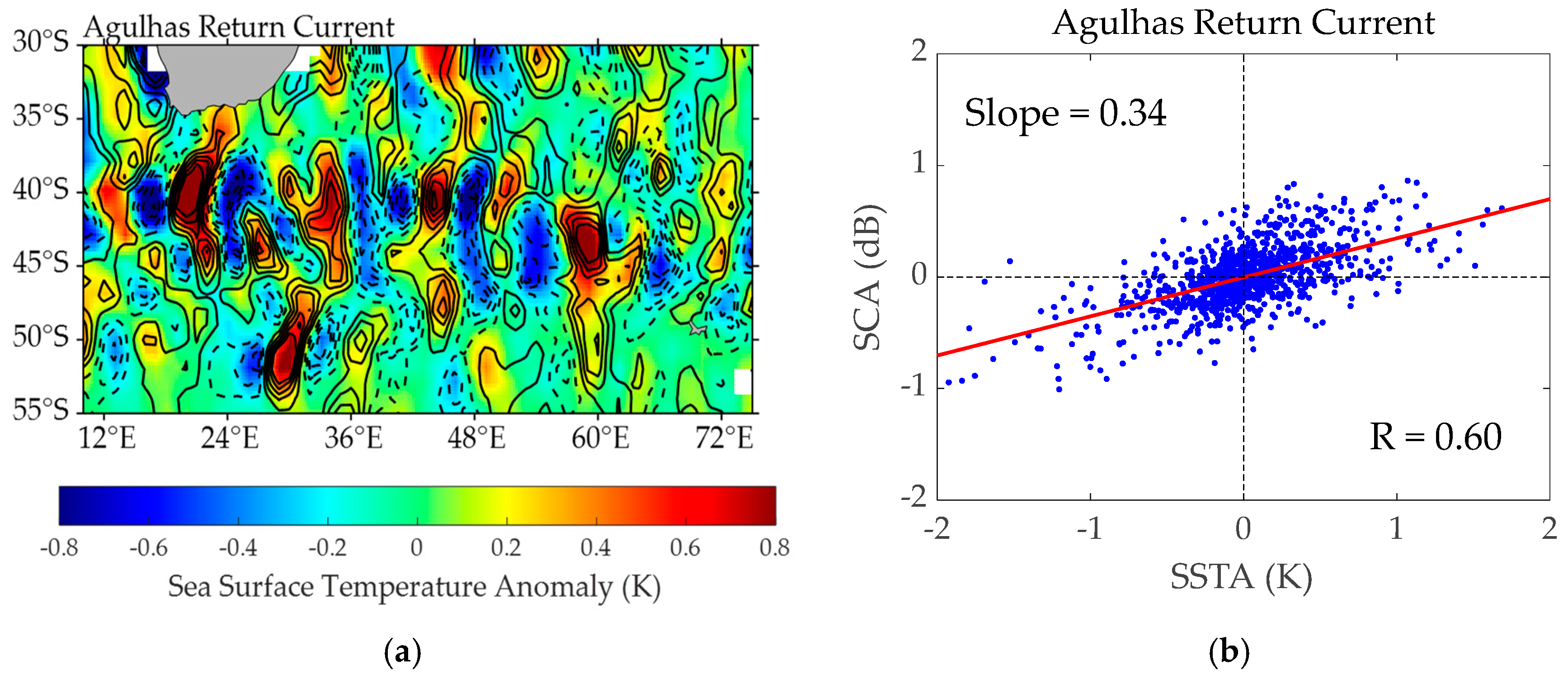
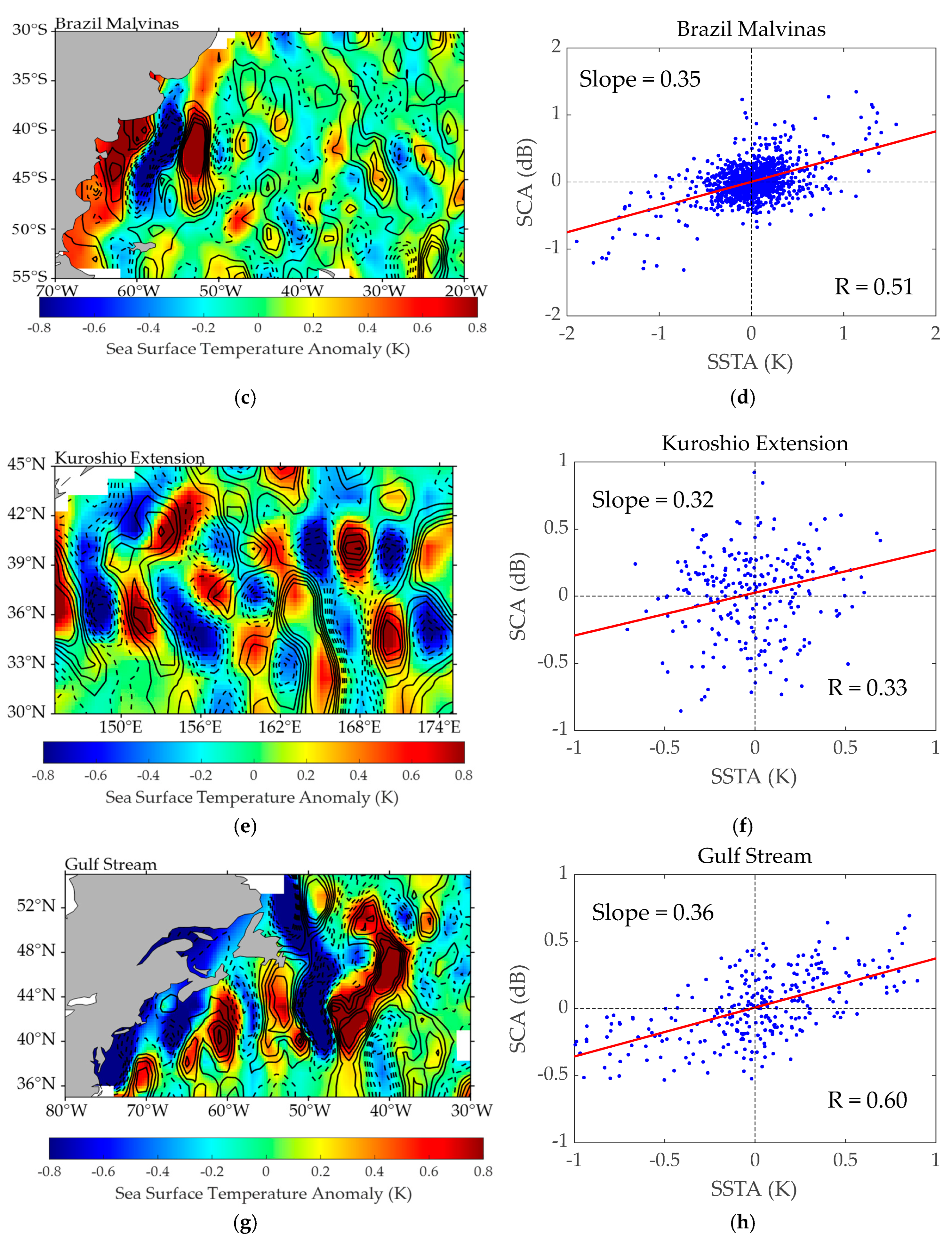
3.2.1. The Response Relationship Between the SSTA and SCA

As an example, the maps of the SSTA (colors) and SCA (contours) fields over the four typical sea areas are shown in the left images of Figure 5. And the corresponding scatter plots are presented in the right images of Figure 5. The x-axis of the scatter plots represents the SSTA, while the y-axis represents the SCA. In the Southern Hemisphere (i.e., ARC and BMC), the data in January 2005 were used. In the Northern Hemisphere (i.e., KE and GS), the data in June of the same year were employed. The reasons for choosing different data dates for the Southern and Northern Hemispheres are explained in the subsequent section. Just as expected, the SCA is positively correlated with the SSTA, i.e., the larger (smaller) scattering coefficient is over the warmer (colder) water. The scatter plot shows a moderate correlation between the SSTA and SCA. The correlation coefficients are 0.60, 0.51, 0.33, and 0.60 in the four sea areas, respectively. Based on the definition, the slope of the fit line in Figure 5 represents the coupling coefficient between the SSTA and SCA. And the values of the coupling coefficient $k_{ssta}$ in the ARC, BMC, KE, and GS regions are 0.34, 0.35, 0.32, and 0.36, respectively. The results in reference [25] showed that the wind speed anomaly is more sensitive to the SATDA than the SSTA. This means that the SATDA maybe has a more significant effect on the SCA than the SSTA.

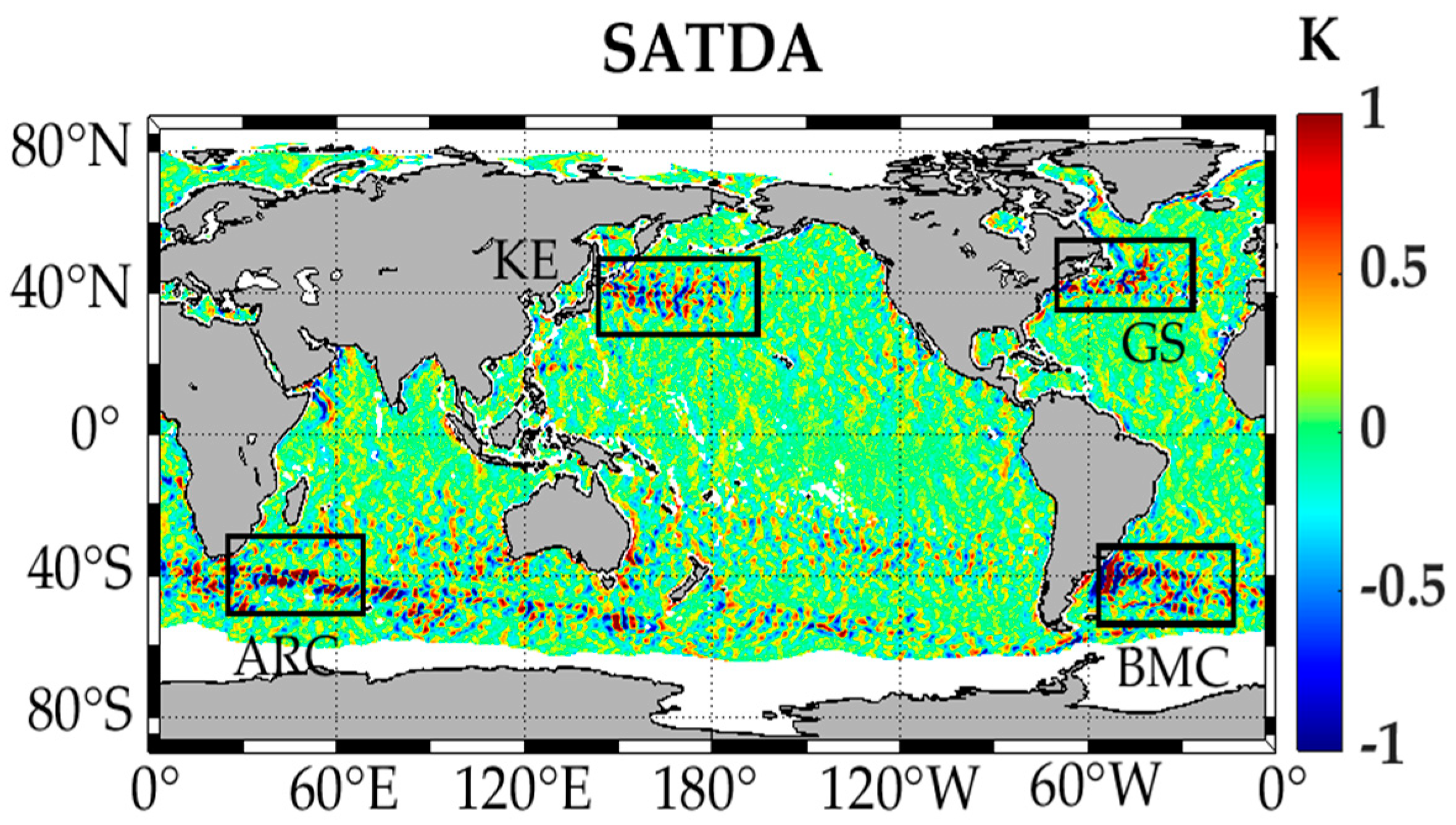
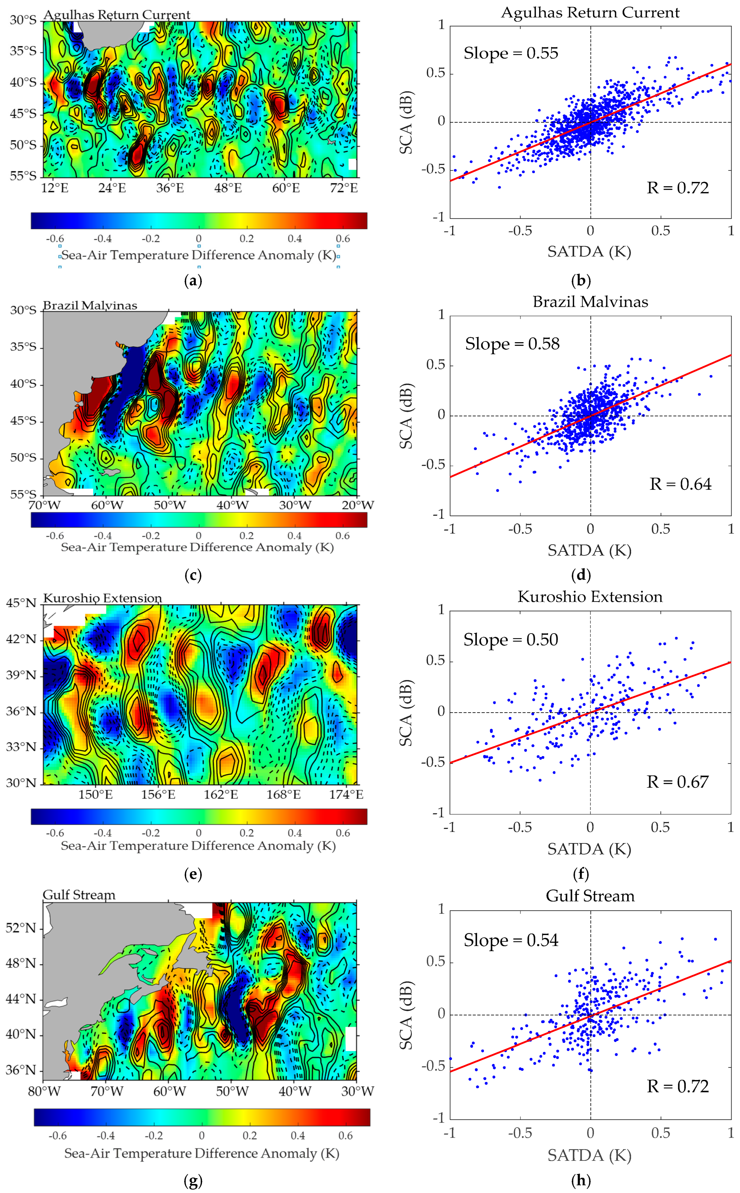
3.2.2. The Response Relationship Between the SATDA and SCA

Figure 6 illustrates the response between the SCA and SATDA in the four typical marine areas. Just as expected, the results in Figure 6 demonstrate that the values of the coupling coefficient $k_{satda}$ and the correlation coefficients between the SCA and SATDA over the four typical marine areas are all obviously larger than those in Figure 5. For example, the value of the coupling coefficient in the ARC region increased from 0.34 to 0.55, while the correlation coefficient increased from 0.60 to 0.72. This result indicates that the SCA is more sensitive to the SATDA than the SSTA.

In order to further demonstrate the influence of SATD and SST on the scattering coefficient in the four typical sea areas, the long-term variation characteristics of coupling coefficients $k_{satda}$ and $k_{ssta}$ from January 2002 to June 2009 are shown in Figure 7. From the comparison between $k_{ssta}$ and $k_{satda}$, one can find that the values of $k_{satda}$ are significantly larger than those of $k_{ssta}$. On the other hand, we also find that the values of $k_{satda}$ and $k_{ssta}$ exhibit seasonal variation. In the four sea regions, the coupling coefficients $k_{satda}$ and $k_{ssta}$ reach the maximum values in summer (December and January in the Southern Hemisphere, and July and August in the Northern Hemisphere) and the minimum values in winter (July and August in the Southern Hemisphere, and December and January in the Northern Hemisphere).

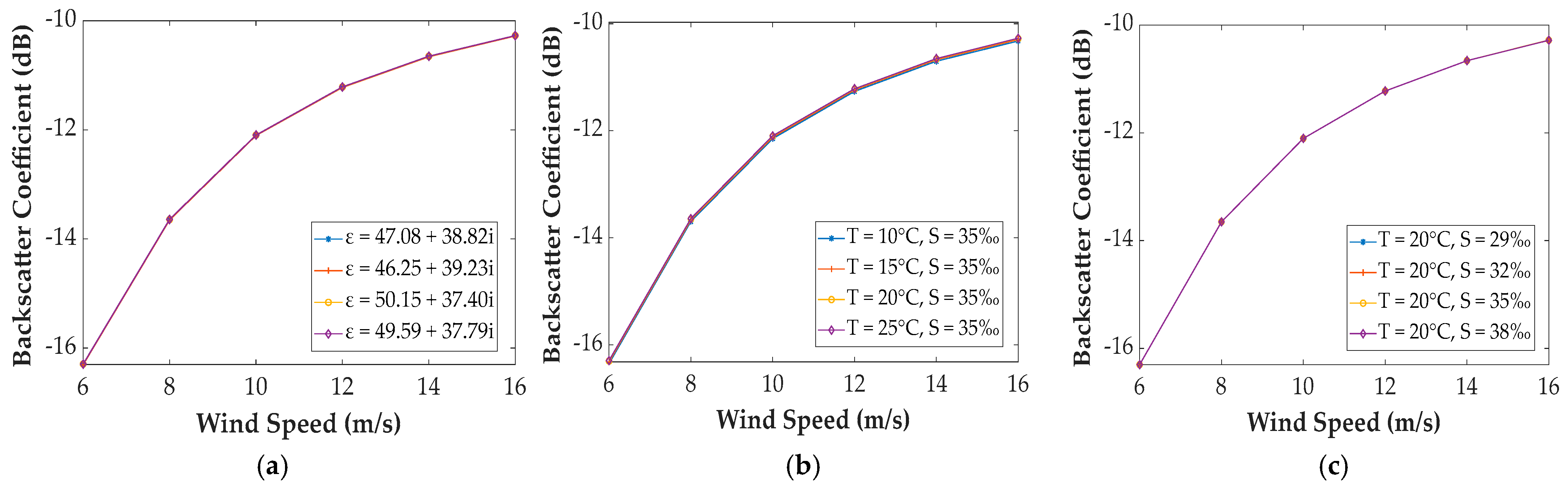
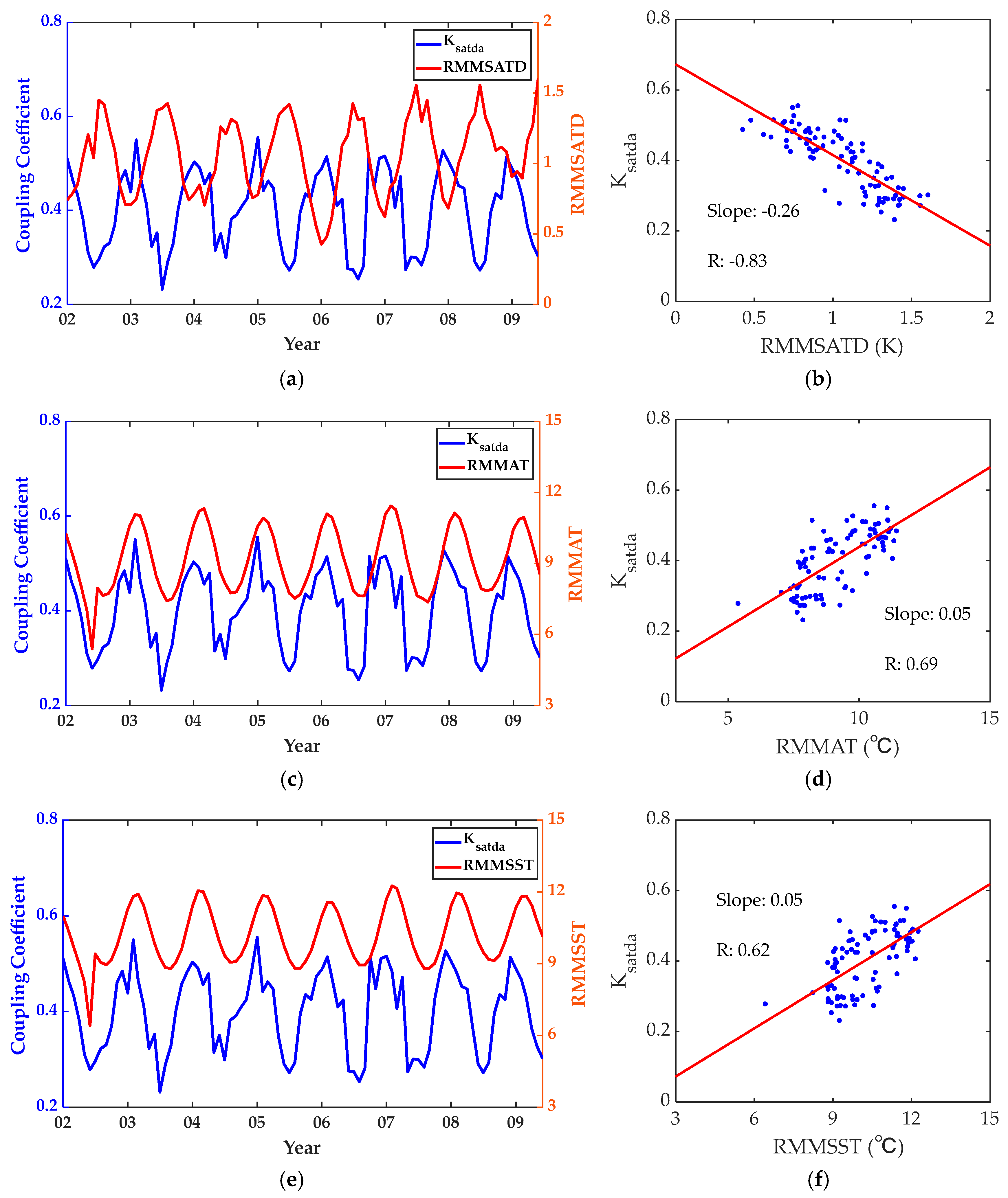
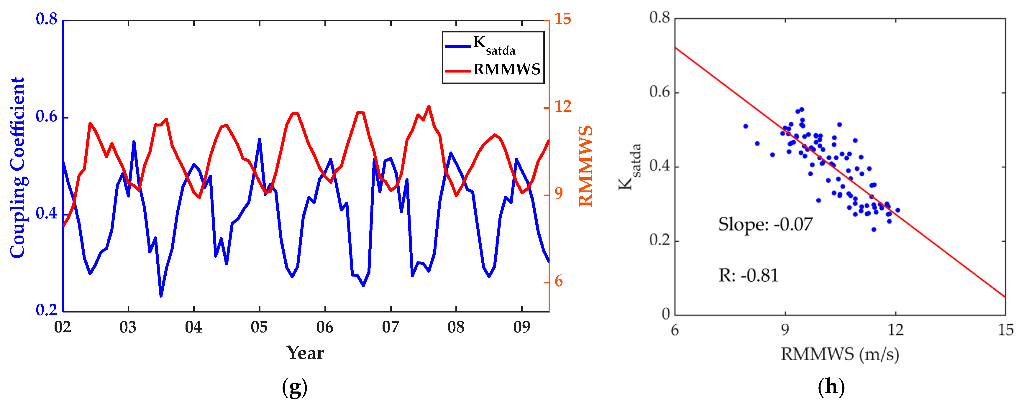
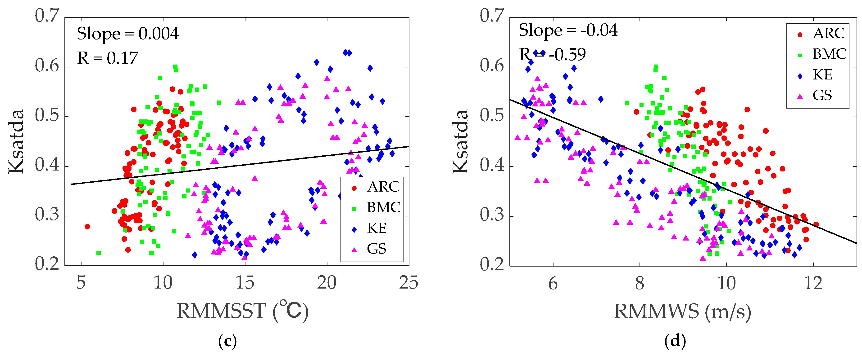
3.3. The Impact of the Marine Environmental Parameters on $k_{satda}$

As discussed in the previous section, the SCA is more sensitive to the SATDA than the SSTA, and the coupling coefficient $k_{satda}$ is greater than $k_{ssta}$. Therefore, the following discussion focuses solely on the impacts of environmental parameters on the coupling coefficient $k_{satda}$. In order to reveal the reason why the coupling coefficient $k_{satda}$ varies with the seasons, the influence of the background marine environment on $k_{satda}$ is analyzed using the data from January 2002 to June 2009.

As an example, the curves of the RMMSATD, RMMAT, RMMSST, and RMMWS in the ARC region varying with seasons are shown in Figure 8. Here, RMMSATD, RMMAT, RMMSST, and RMMWS denote the values of the regional monthly mean SATD, regional monthly mean air temperature, regional monthly mean SST, and regional monthly mean wind speed over the ARC region and can be considered the background environmental parameters. The corresponding scatter plots of the coupling coefficient and the environmental parameters are shown in Figure 8. From Figure 8, it is found that there are correlations between $k_{satda}$ and the background environmental parameters. Figure 8 illustrates that $k_{satda}$ exhibits a negative correlation with RMMSATD and RMMWS, while showing a positive correlation with RMMAT and RMMSST. And the absolute value of the correlation coefficient between $k_{satda}$ and RMMSATD is the largest. In our work, the statistic correlation coefficients between the coupling coefficient and the background environmental parameters in the other three typical sea areas have also been evaluated, and similar conclusions can be found.

To further analyze which background environmental parameter primarily affects the coupling coefficient $k_{satda}$, the scatter plots of $k_{satda}$ varying with these parameters over the four regions are plotted together in Figure 9. The solid lines in Figure 9 denote the fitting lines based on the overall data of the four regions. When the data over the four typical sea areas are all considered, the results in Figure 9 show that the coupling coefficient $k_{satda}$ has the strongest correlation with RMMSATD, with a correlation coefficient of −0.81. Comparing the correlation coefficient with that in Figure 8, the value of the correlation coefficient between $k_{satda}$ and RMMSATD remains almost unchanged. However, the absolute values of the correlation coefficients between $k_{satda}$ and the other three oceanic environmental parameters (i.e., RMMAT, RMMSST, and RMMWS) all decrease significantly. These results show once again that RMMSATD is the key parameter affecting the coupling coefficient $k_{satda}$.

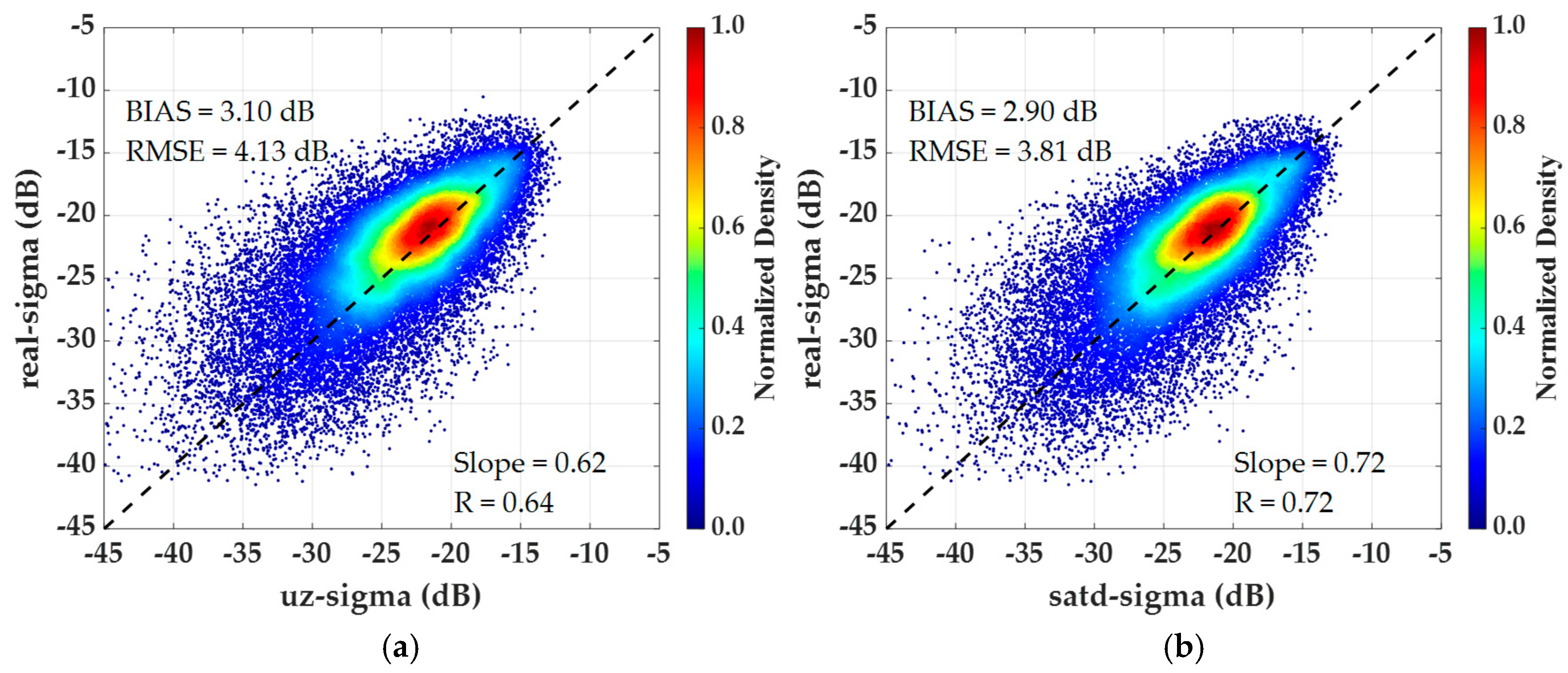
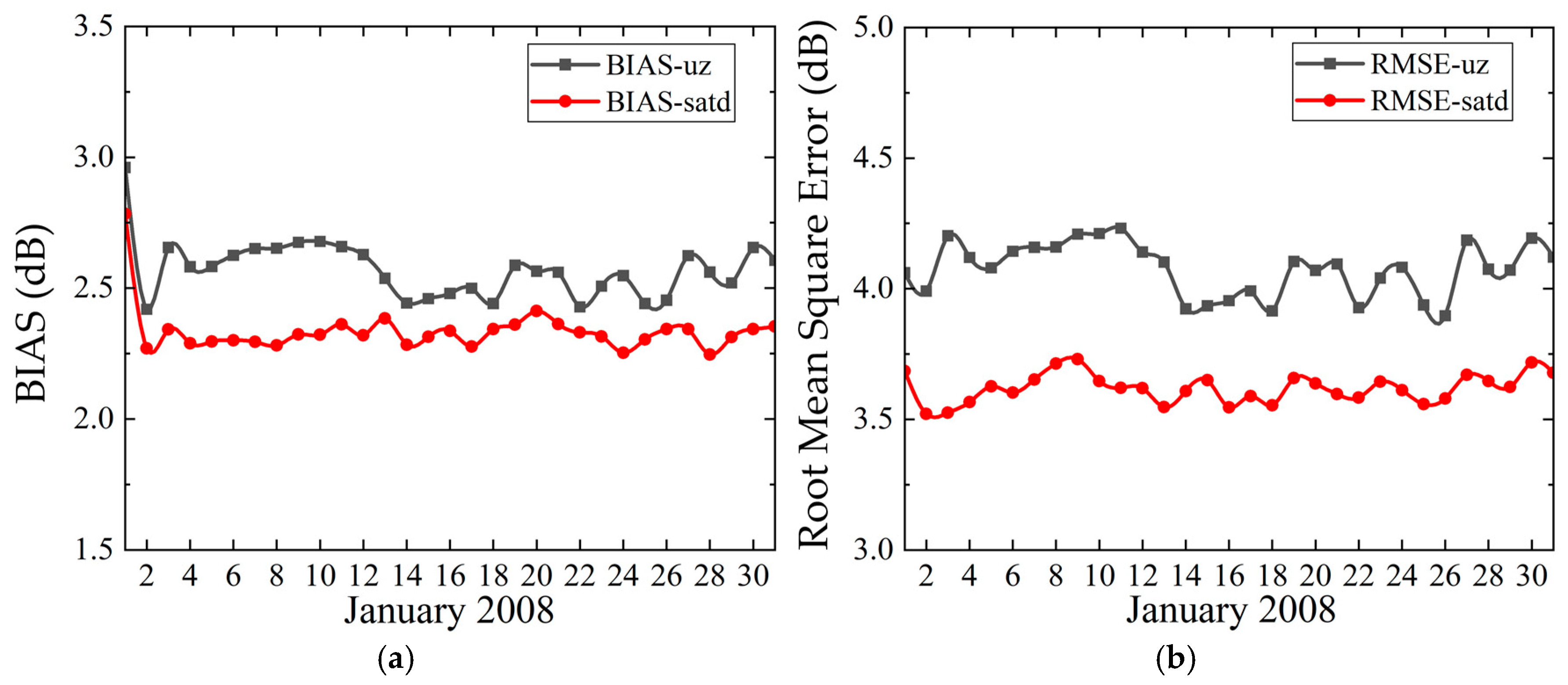
3.4. Improving the Scattering Coefficient Accuracy by Introducing SATD

The traditional geophysical model function (GMF) primarily depends on wind speed, wind direction, and incident angle, without considering the effect of SATD. This omission would limit the accuracy of the scattering coefficient evaluated by the GMF. In this section, the influence of SATD on the accuracy of the GMF is analyzed.

The QSCAT scatterometer operates in the Ku–band; therefore, the Ku–band GMF is used for the calculation of the scattering coefficient. Figure 10 displays the global scattering coefficient data on 1 January 2008. In Figure 10, the vertical axis (real–sigma) represents the scattering coefficient measured by the QSCAT, while the horizontal axis uz–sigma in Figure 10a and satd–sigma in Figure 10b denote the scattering coefficients evaluated by the Ku-band GMFs with and without considering the influence of SATD on the ECMWF wind speed. Comparing the values of the BIAS and the RMSE in Figure 10b with those in Figure 10a, we can find that the accuracy of the scattering coefficient calculated by the GMFs can be improved when the influence of SATD is considered.

The ECMWF wind speed, SATD, and scattering coefficient acquired by the QSCAT in January 2008 were employed to further evaluate the BIAS and the RMSE of the scattering coefficient calculated by the GMFs with and without considering the effect of SATD on the ECMWF wind speed. As shown in Figure 11, it can be observed that the BIAS and the RMSE decrease by about 0.5 dB and 0.7 dB when the effect of SATD on the ECMWF wind speed is considered. This result validates that the accuracy of the scattering coefficient calculated by the GMFs and can be improved by introducing the impact of SATD.

4. Discussion

We studied the response relationship between SATDA and SCA, as well as the response relationship between SSTA and SCA in four typical sea areas (i.e. ARC, BMC, KE and GS) by using data from QSCAT, AMSR-E and ECMWF. The results indicate that SCA is more sensitive to SATDA than SSTA. As shown in Figure 7, the coupling coefficient between SATDA and SCA is significantly higher than that between SSTA and SCA, reaching a maximum of 0.62 in summer and decreasing to 0.2 in winter. This suggests that SATD plays a crucial role in influencing the microwave scattering coefficient. This result is consistent with previous studies on air–sea coupling, indicating that SATD affects the scattering coefficient by influencing wind speed [22,23,25]. We also observed seasonal variations in the values of $k_{satda}$ and $k_{ssta}$. In the four sea regions, the coupling coefficients $k_{satda}$ and $k_{ssta}$ reach their maximum values in summer (December and January in the Southern Hemisphere, and July and August in the Northern Hemisphere) and their minimum values in winter (July and August in the Southern Hemisphere, and December and January in the Northern Hemisphere).

To understand the seasonal variation of the coupling coefficient $k_{satda}$, we analyzed the influence of the background marine environment on $k_{satda}$ using the data from January 2002 to June 2009. The results for the ARC sea area are shown in Figure 8. It can be observed that $k_{satda}$ exhibits a negative correlation with RMMSATD and RMMWS, while showing a positive correlation with RMMAT and RMMSST. And the absolute value of the correlation coefficient between $k_{satda}$ and RMMSATD is the largest. The scatter plots of $k_{satda}$ varying with these parameters over the four regions are plotted together in Figure 9. The results show that the correlation between the $k_{satda}$ and RMMSATD is the strongest, with a correlation coefficient of −0.81. Comparing the correlation coefficient with that in Figure 8, the value of the correlation coefficient between $k_{satda}$ and RMMSATD remains almost unchanged. These results show once again that RMMSATD is the key parameter affecting the coupling coefficient $k_{satda}$.

In order to prove the effect of SATD on the scattering coefficient, we introduced SATD into traditional Ku–band GMF. As shown in Figure 11, it can be observed that the BIAS and the RMSE decrease by about 0.5 dB and 0.7 dB when the effect of SATD on the ECMWF wind speed is considered. This improvement is important for applications such as sea surface wind retrieval. Although the influence of SATD on the microwave scattering coefficient is discussed in this study, the influence of other marine environmental parameters on the scattering coefficient can be further explored in future studies to gain a more comprehensive understanding of the influencing factors of the scattering coefficient.

5. Conclusions

In summary, this study provides a theoretical analysis of the influence of typical oceanic environmental parameters on the microwave scattering coefficient, clearly identifying the SATD as a key parameter affecting the scattering coefficient besides the wind field. Based on the scatterometer, radiometer data, and ECMWF reanalysis data, the response relationships between the SSTA and SCA, as well as between the SATDA and SCA were quantitatively characterized. It was found that the coupling coefficient $k_{satda}$ between the SATDA and SCA is larger and exhibits a seasonal variation, with higher values in summer and lower values in winter. Further quantitative analysis was conducted to examine the correlation between RMMSATD, RMMAT, RMMSST, or RMMWS and $k_{satda}$. The results indicate that RMMSATD exhibits the most significant correlation with $k_{satda}$.

To verify the impact of SATD on the accuracy of the scattering coefficient evaluated by the GMF, the evaluated scattering coefficients with and without considering the effect of SATD have been compared with the scattering coefficients measured by the QSCAT. The values of the BIAS and the RMSE indicate that the accuracy of the scattering coefficient evaluated by the GMFs can be improved by introducing the impact of SATD. It should be noted that this study only focused on the effects of several typical marine atmospheric parameters on the scattering coefficient. In future studies, the effects of the other marine environmental parameters on the scattering coefficient should also be discussed in depth.

References

1. Jafari, Z.; Bobby, P.; Karami, E.; Taylor, R. A Novel Method for the Estimation of Sea Surface Wind Speed from SAR Imagery. J. Mar. Sci. Eng. 2024, 12, 1881. [Google Scholar] [CrossRef]
2. Plant, W.J. A relationship between wind stress and wave slope. J. Geophys. Res. Ocean. 1982, 87, 1961–1967. [Google Scholar] [CrossRef]
3. Hong, S.; Shin, I. Wind speed retrieval based on sea surface roughness measurements from spaceborne microwave radiometers. J. Appl. Meteorol. Climatol. 2013, 52, 507–516. [Google Scholar] [CrossRef]
4. Collard, F.; Mouche, B.; Chapron, B. On the use of Doppler shift for SAR wind retrieval. In Proceedings of the 3rd International Workshop SeaSAR 2010, Frascati, Italy, 25–29 January 2010; pp. 1–8. [Google Scholar]
5. Yang, S.; Zhang, L.; Lin, M.; Zou, J.; Mu, B.; Peng, H. Evaluation of Sea Surface Wind Products from Scatterometer Onboard the Chinese HY-2D Satellite. Remote Sens. 2023, 15, 852. [Google Scholar] [CrossRef]
6. Xie, D.; Chen, K.S.; Yang, X. Effects of wind wave spectra on radar backscatter from sea surface at different microwave bands: A numerical study. IEEE Trans. Geosci. Remote Sens. 2019, 57, 6325–6334. [Google Scholar] [CrossRef]
7. Fung, A.K.; Li, Z.; Chen, K.S. Backscattering from a randomly rough dielectric surface. IEEE Trans. Geosci. Remote Sens. 1992, 30, 356–369. [Google Scholar] [CrossRef]
8. Thorsos, E.I. The validity of the Kirchhoff approximation for rough surface scattering using a Gaussian roughness spectrum. J. Acoust. Soc. Am. 1988, 83, 78–92. [Google Scholar] [CrossRef]
9. Thorsos, E.I.; Jackson, D.R. The validity of the perturbation approximation for rough surface scattering using a Gaussian roughness spectrum. J. Acoust. Soc. Am. 1989, 86, 261–277. [Google Scholar] [CrossRef]
10. Soto-Crespo, J.; Friberg, A.; Nieto-Vesperinas, M. Scattering from slightly rough random surfaces: A detailed study on the validity of the small perturbation method. J. Ootical Soc. Am. A-Opt. Image Sci. Vis. 1990, 7, 1185–1201. [Google Scholar] [CrossRef]
11. Chan, H.; Fung, A.K. A theory of sea scatter at large incident angles. J. Geophys. Res. Atmos. 1977, 82, 3439–3444. [Google Scholar] [CrossRef]
12. Li, J.; Guo, L.; He, Q. Hybrid FE-BI-KA method in analysing scattering from dielectric object above sea surface. Electron. Lett. 2011, 47, 1147–1148. [Google Scholar] [CrossRef]
13. Zhang, B.; Mouche, A.; Lu, Y.; Perrie, W.; Zhang, G. A geophysical model function for wind speed retrieval from C-band HH-polarized synthetic aperture radar. IEEE Geosci. Remote Sens. Lett. 2019, 16, 1521–1525. [Google Scholar] [CrossRef]
14. Stoffelen, A.; Verspeek, J.A.; Vogelzang, J.; Verhoef, A. The CMOD7 geophysical model function for ASCAT and ERS wind retrievals. IEEE J. Sel. Top. Appl. Earth Obs. Remote Sens. 2017, 10, 2123–2134. [Google Scholar] [CrossRef]
15. Kumar, P.; Gairola, R.M. Fostering the need of L-band radiometer for extreme oceanic wind research. IEEE Trans. Geosci. Remote Sens. 2021, 60, 1–6. [Google Scholar] [CrossRef]
16. Ricciardulli, L.; Wentz, F. Reprocessed QuikSCAT (V04) wind vectors with Ku-2011 geophysical model function. In Remote Sensing Systems Technical Report 043011; Remote Sensing Systems: Santa Rosa, CA, USA, 2011. [Google Scholar]
17. Panfilova, M.; Karaev, V. Gale Wind Speed Retrieval Algorithm Using Ku-Band Radar Data Onboard GPM Satellite. Remote Sens. 2022, 14, 6268. [Google Scholar] [CrossRef]
18. Wallace, J.M.; Mitchell, T.P.; Deser, C. The influence of sea-surface temperature on surface wind in the eastern equatorial Pacific: Seasonal and interannual variability. J. Clim. 1989, 2, 1492–1499. [Google Scholar] [CrossRef]
19. Hayes, S.P.; McPhaden, M.J.; Wallace, J.M. The influence of sea-surface temperature on surface wind in the eastern equatorial Pacific: Weekly to monthly variability. J. Clim. 1989, 2, 1500–1506. [Google Scholar] [CrossRef]
20. Chelton, D.B.; Esbensen, S.K.; Schlax, M.G.; Thum, N.; Freilich, M.H.; Wentz, F.J.; Gentemann, C.L.; McPhaden, M.J.; Schopf, P.S. Observations of coupling between surface wind stress and sea surface temperature in the eastern tropical Pacific. J. Clim. 2001, 14, 1479–1498. [Google Scholar] [CrossRef]
21. O’Neill, L.W.; Chelton, D.B.; Esbensen, S.K.; Wentz, F.J. High-resolution satellite measurements of the atmospheric boundary layer response to SST variations along the Agulhas Return Current. J. Clim. 2005, 18, 2706–2723. [Google Scholar] [CrossRef]
22. Monin, A.S.; Jaglom, A.M.; Lumley, J.L. Statistical Fluid Mechanics: Mechanics of Turbulence; MIT Press: Cambridge, MA, USA, 1971. [Google Scholar]
23. Wang, Y.; Wang, Y.; Zhang, Y. The Effects of MSATD and MWS on the Coupling Coefficient Between SATDA And WSA. In Proceedings of the IGARSS 2019—2019 IEEE International Geoscience and Remote Sensing Symposium, Yokohama, Japan, 28 July–2 August 2019; pp. 8117–8120. [Google Scholar]
24. Tang, Z.; Zhang, R.-H.; Wang, H.; Zhang, S.; Wang, H. Mesoscale Surface Wind-SST Coupling in a High-Resolution CESM Over the KE and ARC Regions. J. Adv. Model. Earth Syst. 2021, 13, 1–16. [Google Scholar] [CrossRef]
25. Zhang, Y.; Wang, Y.; Wang, Y.; Bai, Y.; Zhao, C. The influences of environmental factors on the air-sea coupling coefficient. Acta Oceanol. Sin. 2022, 41, 147–155. [Google Scholar] [CrossRef]
26. Wang, Y.; Zhang, Y.; Chen, H.; Guo, L. Effects of atmospheric stability and wind fetch on microwave sea echoes. IEEE Trans. Geosci. Remote Sens. 2013, 52, 929–935. [Google Scholar] [CrossRef]
27. Ulaby, F.T.; Moore, R.K.; Fung, A.K. Microwave Remote Sensing Active and Passive-Volume II: Radar Remote Sensing and Surface Scattering and Enission Theory; Addison-Wesley: New York, NY, USA, 1982; pp. 922–982. [Google Scholar]
28. Ellison, W.; Balana, A.; Delbos, G.; Lamkaouchi, K.; Eymard, L.; Guillou, C.; Prigent, C. New permittivity measurements of seawater. Radio Sci. 1998, 33, 639–648. [Google Scholar] [CrossRef]
29. Liu, Q.; Weng, F.; English, S.J. An improved fast microwave water emissivity model. IEEE Trans. Geosci. Remote Sens. 2010, 49, 1238–1250. [Google Scholar] [CrossRef]
30. Elfouhaily, T.; Chapron, B.; Katsaros, K.; Vandermark, D. A Unified Directional Spectrum for Long and Short Wind-Driven Waves. J. Geophys. Res. 1997, 102, 15781–15796. [Google Scholar] [CrossRef]
31. Hwang, P.A. Observations of swell influence on ocean surface roughness. J. Geophys. Res. Ocean. 2008, 113, C12024. [Google Scholar] [CrossRef]
32. Hwang, P.A. A note on the ocean surface roughness spectrum. J. Atmos. Ocean. Technol. 2011, 28, 436–443. [Google Scholar] [CrossRef]
33. Sweet, W.; Fett, R.; Kerling, J.; La Violette, P. Air-Sea Interaction Effects in the Lower Troposphere Across the North Wall of the Gulf Stream. Mon. Weather Rev. 1981, 109, 1042–1052. [Google Scholar] [CrossRef]
34. Li, Y.; Xue, H.; Bane, J.M. A 3D Coupled Atmosphere-Ocean Model Study of Air-Sea Interactions during a Passing Winter Storm over the Gulf Stream. Mon. Weather Rev. 2001, 128, 973–996. [Google Scholar]
35. Galbraith, P.S.; Larouche, P.; Chasse, J.; Petrie, B. Sea-surface temperature in relation to air temperature in the Gulf of St. Lawrence: Interdecadal variability and long term trends. Deep Sea Res. Part II Top. Stud. Oceanogr. 2012, 77, 10–20. [Google Scholar] [CrossRef]
36. Liu, W.T.; Xie, X. Ocean-atmosphere momentum coupling in the Kuroshio Extension observed from space. J. Oceanogr. 2005, 64, 631–637. [Google Scholar] [CrossRef]
37. Koseki, S.; Watanabe, M. Atmospheric Boundary Layer Response to Mesoscale SST Anomalies in the Kuroshio Extension. J. Clim. 2010, 23, 2492–2507. [Google Scholar] [CrossRef]
38. Xu, M.; Xu, H. Atmospheric Responses to Kuroshio SST Front in the East China Sea under Different Prevailing Winds in Winter and Spring. J. Clim. 2015, 28, 3191–3211. [Google Scholar] [CrossRef]
39. Tokinaga, H.; Tanimoto, Y.; Xie, S.P. SST-Induced Surface Wind Variations over the Brazil-Malvinas Confluence: Satellite and In Situ Observations. J. Clim. 2005, 18, 3470–3482. [Google Scholar] [CrossRef]
40. Souza, R.; Pezzi, L.; Swart, S.; Oliveira, F.; Santini, M. Air-sea interactions over eddies in the Brazil-Malvinas confluence. Remote Sens. 2021, 13, 1335. [Google Scholar] [CrossRef]
41. De Freitas, R.A.P.; de Souza, R.B.; Reis, R.A.d.N.; de Mendonca, L.F.F.; da Silva Lindermann, D. Satellite and in situ measurements of water vapour in the Brazil-Malvinas Confluence region. Int. J. Climatol. 2024, 44, 4286–4305. [Google Scholar] [CrossRef]
42. Rouault, M.; Leethorp, A.M.; Lutjeharms, J.R.E. The Atmospheric Boundary Layer above the Agulhas Current during a long current Winds. J. Phys. Oceanogr. 2010, 30, 40–50. [Google Scholar] [CrossRef]
43. De Leon, S.; Soares, C.G. Numerical study of the effect of current on waves in the Agulhas Current Retroflection. Ocean Eng. 2022, 264, 112333–112343. [Google Scholar] [CrossRef]
44. Arne, B.; Ruhs, S.; Ivanciu, I.; Žschwarzkopf, F.U.; Veitch, J.; Reason, C.; Zorita, E.; Tim, N.; Hunicke, B.; Vafeidis, A.T.; et al. The Agulhas Current System as an Important Driver for Oceanic and Terrestrial Climate. In Sustainability of Southern African Ecosystems Under Global Change: Science for Management and Policy Interventions; Springer International Publishing: Cham, Switzerland, 2024; pp. 191–220. [Google Scholar]
45. Hoffman, R.N.; Leidner, S.M. An introduction to the near–real–time QuikSCAT data. Weather Forecast. 2005, 20, 476–493. [Google Scholar] [CrossRef]
46. Lungu, T.; Callahan, P.S. QuikSCAT Science Data Product User’s Manual: Overview and Geophysical Data Products, D-18053-Rev A, Version 3; NASA: Washington, DC, USA, 2006. [Google Scholar]
47. Nakata, K.; Ohshima, K.I.; Nihashi, S. Estimation of thin-ice thickness and discrimination of ice type from AMSR-E passive microwave data. IEEE Trans. Geosci. Remote Sens. 2018, 57, 263–276. [Google Scholar] [CrossRef]
Figure 1. (a) Effects of SATD on scattering coefficient at different wind speeds. (b) First–order derivative of scattering coefficient versus SATD at different wind speeds.
Remotesensing 17 01405 g001
Figure 2. Changes in scattering coefficient under different conditions of (a) permittivity of seawater, (b) sea surface temperature, and (c) seawater salinity.
Remotesensing 17 01405 g002
Figure 3. Schematic diagram of the scattering coefficient calibration.
Remotesensing 17 01405 g003
Figure 4. The four typical sea areas studied in this paper. The map illustrates the sea–air temperature difference anomaly in August 2015.
Remotesensing 17 01405 g004
Figure 5. The map of the SCA overlaid as contours on the SSTA at the (a) ARC, (c) BMC, (e) KE, and (g) GS, and the scatter plot distribution of data for the (b) ARC, (d) BMC, (f) KE, and (h) GS sea areas.
Remotesensing 17 01405 g005aRemotesensing 17 01405 g005b
Figure 6. The map of the scattering coefficient anomaly overlaid as contours on the sea–air temperature difference anomaly at the (a) ARC, (c) BMC, (e) KE, and (g) GS, and the scatter plot distribution of data for the (b) ARC, (d) BMC, (f) KE, and (h) GS sea areas.
Remotesensing 17 01405 g006
Figure 7. Comparisons of the interannual variations in the coupling coefficients k s a t d a and k s s t a in the four sea areas, namely the (a) ARC, (b) BMC, (c) KE, and (d) GS sea areas, from January 2002 to June 2009.
Remotesensing 17 01405 g007
Figure 8. Relationships between the coupling coefficient k s a t d a and various oceanic environmental parameters in the ARC region from January 2002 to June 2009. The variation curves of the coupling coefficient k s a t d a with (a) RMMSATD, (c) RMMAT, (e) RMMSST, and (g) RMMWS, as well as the scatter plots of k s a t d a with (b) RMMSATD, (d) RMMAT, (f) RMMSST, and (h) RMMWS.
Remotesensing 17 01405 g008aRemotesensing 17 01405 g008b
Figure 9. The distribution of the comprehensive scatter plots of the different regional monthly mean marine environmental parameters, (a) RMMSATD, (b) RMMAT, (c) RMMSST, and (d) RMMWS, and the coupling coefficient k s a t d a in the four sea areas. The red dots represent the ARC sea area, the green square dots represent the BMC sea area, the blue diamonds represent the KE sea area, and the rose-red triangles represent the GS sea area.
Remotesensing 17 01405 g009aRemotesensing 17 01405 g009b
Figure 10. The comparison between the QSCAT–measured scattering coefficient and the scattering coefficient calculated using the (a) ECMWF wind speed and (b) ECMWF wind speed with a sea–air temperature difference correction.
Remotesensing 17 01405 g010
Figure 11. The inter–month variation curves of the BIAS (a) and the RMSE (b) of the scattering coefficient calculated based on GMFs with and without considering the effect of SATD on the ECMWF wind speed.
Remotesensing 17 01405 g011
Disclaimer/Publisher’s Note: The statements, opinions and data contained in all publications are solely those of the individual author(s) and contributor(s) and not of MDPI and/or the editor(s). MDPI and/or the editor(s) disclaim responsibility for any injury to people or property resulting from any ideas, methods, instructions or products referred to in the content.