Abstract
As part of the Copernicus program of the European Union (EU), the European Space Agency (ESA) and the European Organisation for the Exploitation of Meteorological Satellites (EUMETSAT) are currently operating the Sentinel-3 mission that consists of a constellation of two unites A and B (S3A, S3B). Each unit carries on board an Ocean and Land Colour Instrument (OLCI) that is acquiring moderate-spatial-resolution optical imagery. This article provides a description of the Level-1B radiometry product validation activities of the constellation Sentinel-3A and Sentinel-3B after six years in orbit. Several vicarious calibration methods have been applied independently by three expert groups and the results are compared over different surface target types. All methods agree on the good radiometric performance of both instruments. Although OLCI-A shows brighter Top-of-Atmosphere (TOA) radiance than OLCI-B by about 1–2%, both sensors exhibit very good stability and good image quality. The results are analyzed and discussed to propose a set of vicarious gain coefficients that could be used to align OLCI-A with OLCI-B radiometry time-series. Finally, recommendations for future missions are suggested.
Keywords:
calibration; validation; optical; instrument; processing; imagery; radiometry; Sentinel-3; OLCI 1. Introduction
The European Union’s Copernicus program has seen the development and operation of Sentinel-3. The mission is operated by EUMETSAT with the objective of producing measurements to study global environmental issues on the land and sea by providing geophysical quantities to drive numerical prediction models at the global–regional scales, ultimately supporting Copernicus user needs [1].
Sentinel-3 is a constellation mission consisting of twin satellites, both in a sun-synchronous, near-polar orbit at around 814 km, with a descending node of 10:00am local time. Aboard these satellites is the Ocean and Land Colour Instrument (OLCI). OLCI is a push-broom imaging spectrometer with a fan-shaped array of five cameras with a native 300 m spatial resolution across a 1270 km swath in 21 spectral bands ranging from 400 to 1020 nm. The mission’s ability to provide good data quality in terms of radiometry and fidelity is of paramount importance across a wide range of applications. Such qualities are key for enabling the exploitation of time-series, inter-comparison of measurements across different sensors, and observing change detection. Validation of the mission is crucial and involves assessing on-ground configuration parameters and algorithms, helping to ensure the data quality is meeting the user and mission requirements. There have been many works studying the OLCI Level-1 radiometric performance, including studies based on the tandem-phase project [2,3,4], and shortly after the launch of Sentinel-3B where cross-comparisons showed good stability [5]. These works point to a bias of 1–2% of TOA signal when comparing the two OLCI units, where the OLCI-A TOA is brighter than OLCI-B.
Therefore, any harmonization efforts with the two sensors would depend on the individual in-flight calibration of both sensors. However, supporting works suggest the inter-calibration ratios will drift over the mission’s lifetime. Therefore, a long-term stability analysis could monitor the sensors’ calibration differences. At the time of writing, we cannot identify any work or study that analyzes the OLCI Level-1 radiometric performance or temporal stability over 5 years since both units have been operational, other than data quality reports (DQRs: https://sentinel.esa.int/web/sentinel/copernicus/sentinel-3/quality, accessed on 20 March 2025).
This work will describe radiometric validation activities over the last six years for the Sentinel-3 mission. Radiometric performance and its subsequent temporal stability have been estimated for Top-of-Atmosphere reflectance products (referred to as Level-1B and further described in this paper) for the full extent of the mission. This paper is structured as follows: Section 1 provides an introduction, followed by Section 2, which describes the materials and methods used in this study. Section 3 presents the results; Section 4 discusses the findings, with Section 5 containing the final conclusion.
2. Materials and Methods
2.1. OLCI Overview
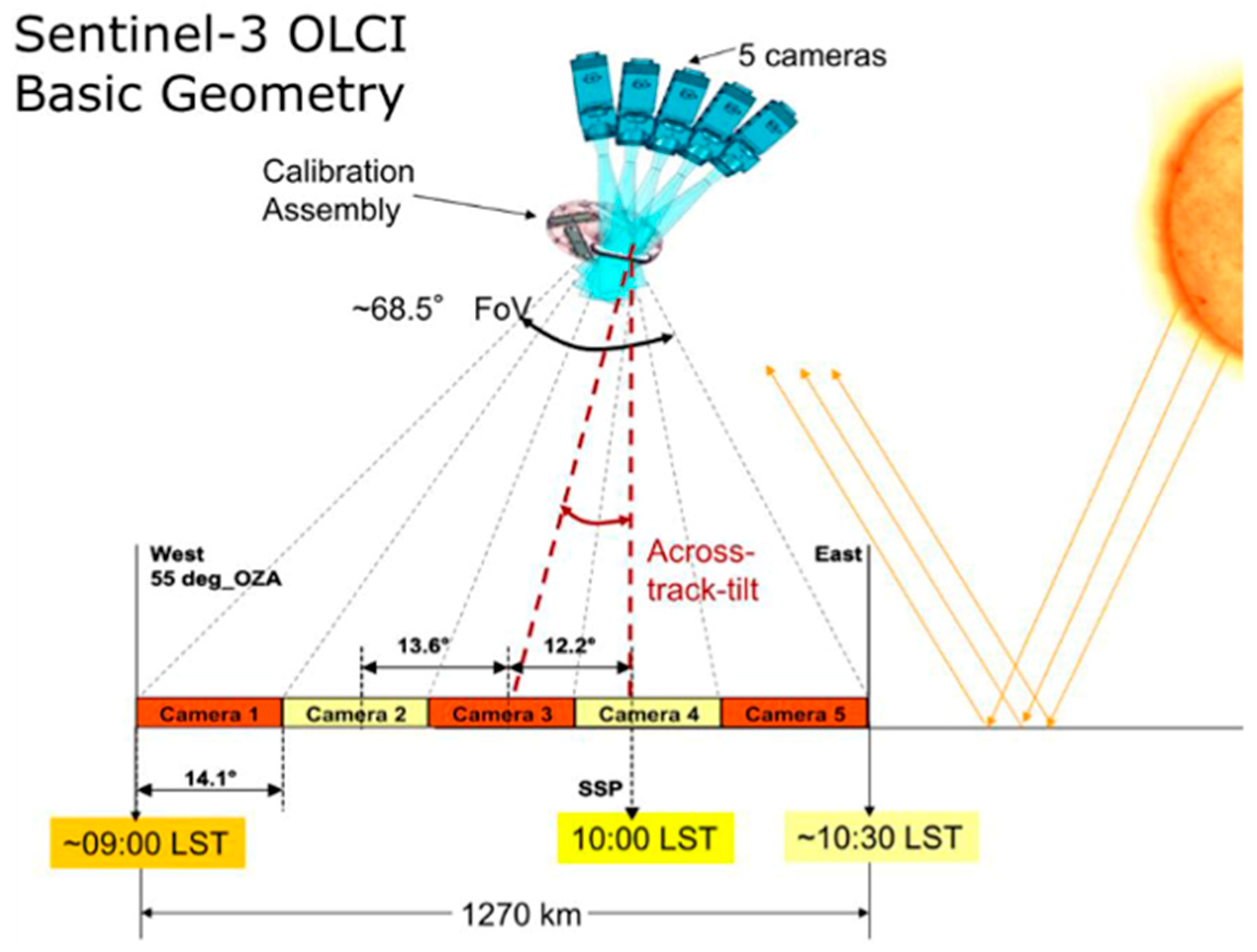
The OLCI follows the design of the opto-mechanical features and imaging of ENVISAT’s MERIS instrument with an adjusted camera arrangement and improved on-board processing capabilities [1]. OLCI uses a push-broom configuration, with 5 camera modules spanning the FOV (Figure 1):
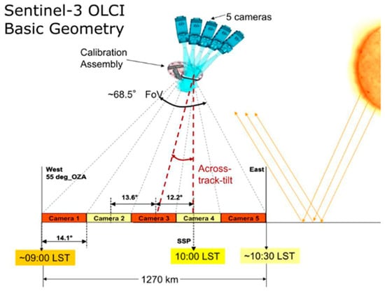
Figure 1.
OLCI basic geometry (extracted from Copernicus Sentinel-3 OLCI Land User Handbook [6]). Note the calibration assembly allowing the insertion of solar diffusers or a shutter into the instrument field of view.
- The five cameras are configured in a fan shape across the FOV in the vertical plane perpendicular to the platform velocity.
- Each individual camera’s 14.2° FOV has a 0.6° overlap with neighboring camera modules.
- To minimize the impact of sunglint, the FOV of the whole array is shifted across-track by 12.58°, away from the sun.
OLCI images the Earth over a 44 min window on the descending path (daytime) of each orbit, with observation beginning when the sun zenith angle (SZA) at the sub-satellite point goes below 80° and stopping once it again reaches 80°. The 68.5 FOV and 1270 km swath width mean the global coverage revisit for the Sentinel-3 constellation is 1.1 days at the equator, and 2.2 days for a single satellite. These revisit times decrease as latitude increases due to orbital convergence [7]. The OLCI is a programmable, medium-spatial-resolution imaging spectrometer, sensing in the reflective solar spectral range in twenty-one spectral bands (390–1040 nm). These bands are programmable from the ground in width and position in 1.25 nm steps (Table 1) [1]. The 1270 km field of view is shared between five identical cameras with a slightly overlapped configuration, where each camera is covering a 14° field of view.

Table 1.
OLCI band characteristics.
On-board radiometric calibration of OLCI is performed using two identical sun-lit diffuser plates when at the orbital south pole. A diffuser is deployed and exposed to sunlight, whilst brought into the FOV of the instrument. Consequently, the radiometric calibration depends on the on-ground characterization of these diffusers, which acts as an on-board secondary reflectance standard.
The dark offset is measured just before thanks to a shutter and provides the second point of the calibration line. OLCI radiometric calibration observations are collected about every two to three weeks using the nominal diffuser. The stability of the nominal diffuser plate is monitored using a reference plate deployed only about every 3 months [7]. Each of the OLCI camera modules is equipped with a polarization scrambling window, aimed at reducing the sensor’s sensitivity to incoming light polarization to a fraction of a percent [1]. The evolution of the instrument sensitivity, as well as the on-orbit aging of the nominal diffuser, are regularly reported in monthly and annual data quality reports (DQRs, available at https://sentiwiki.copernicus.eu/web/document-library#DocumentLibrary-OLCILatestAnnualReports, accessed on 20 March 2025).
2.2. Level-1B Product Overview
Sentinel-3 OLCI Level-1B products are provided as ortho-geolocated, calibrated Top-of-Atmosphere radiances. These measurements are re-gridded onto regular along- and across-track grids. The products are available in versions according to their spatial resolutions: 0.3 km as Full Resolution (FR) and 1.2 km as Reduced Resolution (RR). TOA radiances are accompanied by a variety of flags and attributes such as quality and classification, meteorological information, illumination and acquisition angles, spectral information, per-pixel prognostic uncertainty, timestamps, geolocation, and references to the at-sensor acquisition grid. These products are used for validation and quality control activities.
The Copernicus Sentinels Optical Mission Performance Cluster (Opt-MPC) utilizes two services to subset and collect Level-1B data from the CalVal sites for further validation activities. S3ETRAC [8] extracts valid data from Full Resolution products, and the Data Products Extractor module spatially sub-samples Reduced Resolution products for downstream activities.
2.3. Absolute Radiometry Vicarious Validation
The absolute radiometric calibration relies on the on-board solar diffuser [1]. The vicarious calibration serves to verify the on-board calibration process, whilst distinguishing between the degradation of the sensor and the diffuser aging. Vicarious calibration consists of equivalent TOA radiance computation for a known surface reflectance and known geometric and atmospheric conditions. The calibration gain coefficients are given as the ratio between the TOA observed reflectance and the computed equivalent TOA reflectance for the different bands. The radiometry vicarious verification or validation relies on the following methods: the desert PICS (Pseudo-Invariant Calibration Sites), the Rayleigh scattering method, and the sunglint method (detailed below).
2.3.1. Pseudo-Invariant Calibration Site over Desert
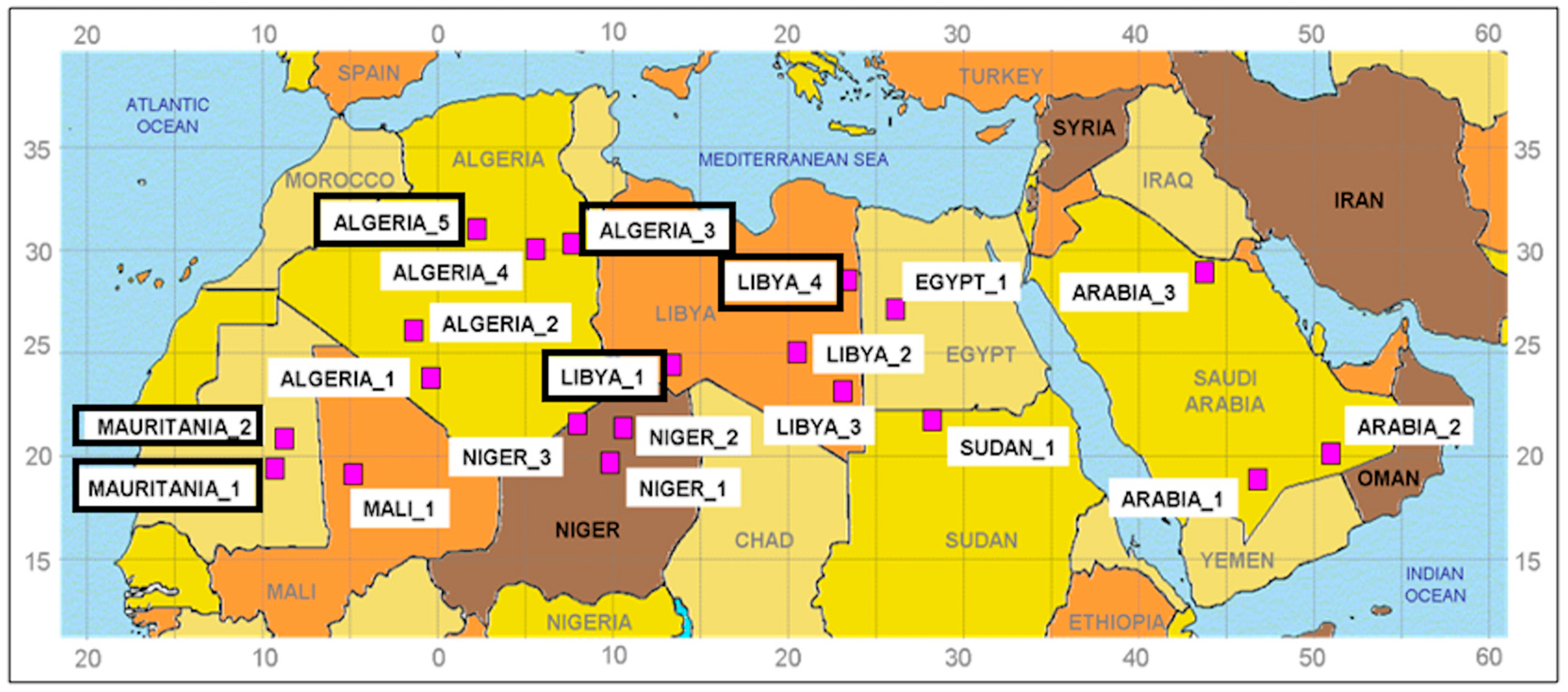
Since the 1980s, desert PICS have been used for multi-temporal radiometry monitoring, as well as sensors’ cross-calibration in the solar spectral range [9]. In general, vicarious calibration methods seek to simulate the TOA reflectance over pre-defined desert sites (e.g., CEOS PICS (http://calvalportal.ceos.org, accessed on 20 March 2025), Figure 2) in the visible to near-infrared (VNIR) up to the short-wave infrared (SWIR) spectral range.

Figure 2.
The location of the desert sites used for the SADE/MUSCLE PICS calibration. The sites, whose names are highlighted in black boxes, are the 6 PICS recommended by CEOS and used for DIMITRI PICS calibration.
In principle, inverse radiative transfer models (RTM) are used to propagate the TOA signal over the CalVal site to the surface reflectance so-called Bottom-of-Atmosphere (BOA) signal. Then, the BOA measurement database, with its large acquisition geometries, is either used to generate a bidirectional reflectance distribution function (BRDF) model or is directly compared with the target sensor by selecting observations with similar geometries. It is necessary to take per-sensor spectral responses into account for both the reference and target sensors; therefore, the BOA reflectance must be spectrally interpolated [10].
Basically the TOA simulations are performed with different 1D RTMs, using target observation geometry, exogenous data for the atmospheric conditions (e.g., trace gas column load and aerosol optical depth), and the reference spectral reflectance or BRDF model [10,11,12,13]. An early selection of the PICS was performed by the “Centre National d’Etudes Spatiales” (CNES) [14] using one year of METEOSAT-4 data. The authors recommended 20 PICS, among them 6 being endorsed by CEOS (Figure 2). Recently, several studies revisited the selection of the desert PICS based on the characterization of the temporal variability and spatial uniformity over North African Sahara and Arabian Peninsula Deserts [15,16], among others. A historical overview of the PICS model and some extensions (e.g., ExPICS and APICS) are provided by [17].
2.3.2. Rayleigh Scattering Vicarious Calibration over Ocean Surface
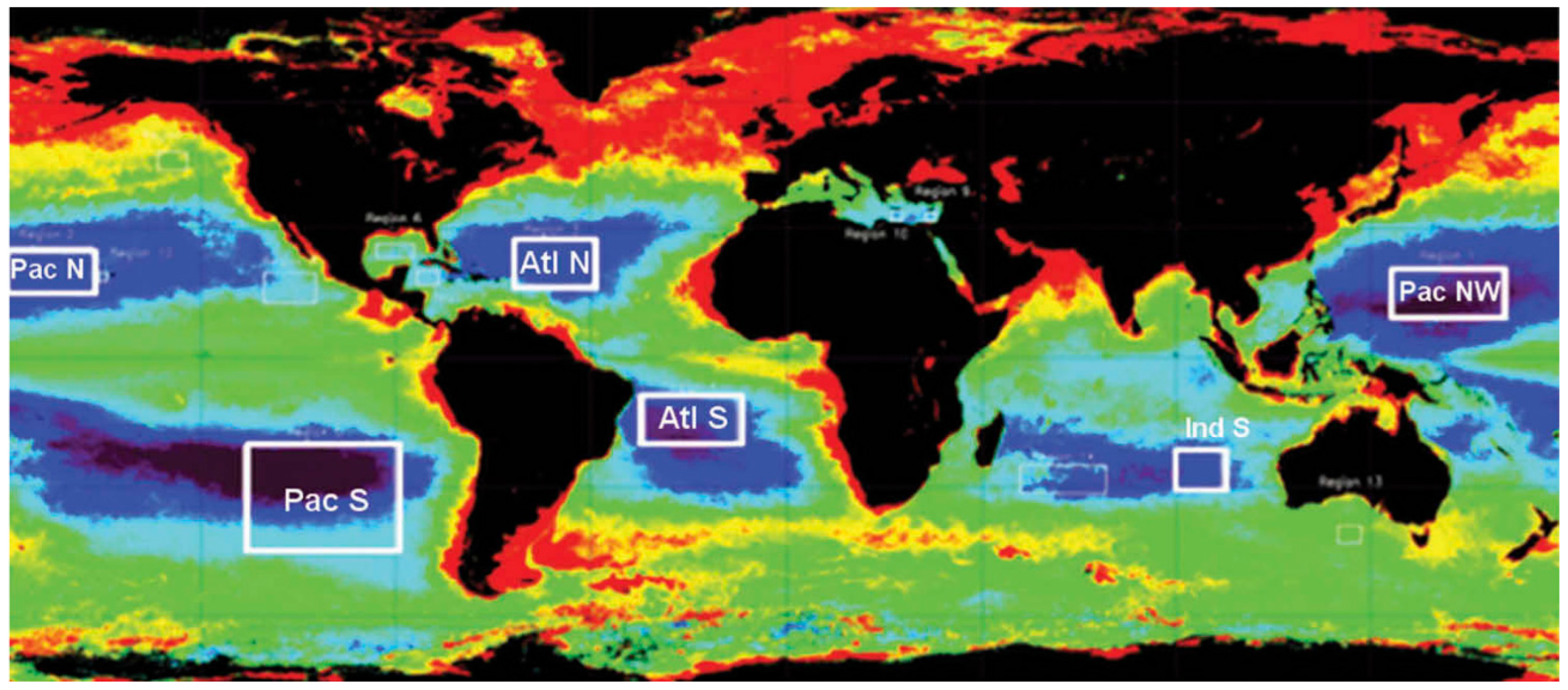
The Top-of-Atmosphere (TOA) signal detected by satellite sensors over oceanic regions primarily results from atmospheric scattering in the visible spectrum [18]. Under optimal conditions—such as stable open oceanic areas with low concentrations of phytoplankton and sediment, and at a significant distance from land (Figure 3)—molecular, or Rayleigh, scattering accounts for around 90% of the TOA signal [19]. Therefore, in open-ocean observations, molecular scattering is the dominant contributor in the visible wavelengths. This scattering is primarily dependent on atmospheric pressure, is well characterized, and can be accurately computed. While the Rayleigh contribution is substantial in the blue wavelength, it decreases significantly towards the near-infrared (NIR). The main contribution at these wavelengths comes from the aerosol scattering (zero marine reflectance) which could be used to estimate the aerosol properties. This assumption is valid for Case 1 waters with low chlorophyll concentration and where phytoplankton is the only optically significant water column contributor [20]. By employing pre-defined aerosol models [21], the aerosol contribution in the NIR can be used to infer this contribution within the visible wavelengths and allow for simulation of the TOA reflectance. Thus, the Rayleigh method uses the comparison of the model-simulated reflectance with the observed reflectance to derive an absolute calibration coefficient as TOA-observed/TOA-simulated.
This approach has been previously used to assess the calibration of SPOT-1 HRV [22] and has been successfully applied to calibrate AVHRR/NOAA and METEOSAT [23,24]. Since then, this method has been applied to several optical missions, from SeaWiFS, POLDER up to MERIS, MODIS, Sentinel-2 and Sentinel-3 [25,26,27,28,29,30,31,32].
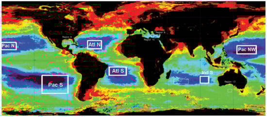
Figure 3.
The six oligotrophic zones used for Rayleigh and sunglint calibration based on [32].
Figure 3.
The six oligotrophic zones used for Rayleigh and sunglint calibration based on [32].
2.3.3. Inter-Band Vicarious Calibration over Sunglint
Sunglint is often used to describe direct specular reflection of light from the water surface. The peak intensity of this reflection on a rough sea surface occurs near the theoretical specular reflection spot that would be observed over a perfect flat sea. Sunglint signature has high reflectance and spectrally flat shape over the spectral range from NIR up to SWIR. This property allows the inter-calibration of spectral bands from one wavelength to those at other wavelengths [28,33]. Essentially, sunglint reflectance depends on both geometric conditions as well as surface roughness. For a flat sea surface (zero wind speed) the specular reflectance or directly reflected light can be computed ‘exactly’ using the Snell–Fresnel laws. Sunglint reflectance over rough surfaces can be predicted using models based on observations, e.g., [34]. The sunglint method typically employs a reference band, often in the red spectrum, to fully characterize the glint signal, irrespective of surface roughness.
Most sunglint correction algorithms utilize signals in the NIR, where water-leaving radiance is considered negligible [35,36]. This method has been successfully applied across various optical satellite missions, particularly ocean-color sensors such as SeaWiFS, MODIS, GLI, MERIS, VIIRS, and OLCI.
2.4. Software and Databases
In this study, we used three independent software/database kits where the aforementioned vicarious calibration methods are implemented and detailed below. The main characteristics (similarities and differences) of these methods are summarized in Table 2.
Table 2.
Summary of the vicarious methods implemented in the three software/database kits used in this study.
2.4.1. DIMITRI Software and Database (ESA, ESTEC, Noordwijk, the Netherlands)
The Database for Imaging Multi-Spectral Instruments and Tools for Radiometric Intercomparison (DIMITRI) is a database of Level-1 products (TOA radiance/reflectance) of optical sensors, coupled with a software offering users the capability of radiometric performance assessment of optical imagers. DIMITRI was initially prototyped at ESA/ESTEC and is currently developed and maintained by ESA, ARGANS, and MAGELLIUM (https://dimitri.argans.co.uk, accessed on 20 March 2025).
DIMITRI offers a suite of tools for the comparison of more than 15 optical sensors over approximately 20 radiometrically homogenous and stable sites at TOA level, within the 400 nm–4 μm wavelength range. The database covers the period 2002 to present. DIMITRI’s interface enables radiometric intercomparisons between sensors or against simulated signals over ocean and cold/hot PICS (e.g., Rayleigh scattering, sunglint and desert/snow PICS methods).
All the available L1B-LN1-NT products from OLCI-A and OLCI-B over the desert CalVal sites (Algeria 3 and 5, Libya 1 and 4, and Mauritania 1 and 2 (Figure 2) and the six ocean CalVal sites (Figure 3)) have been collected over July 2018–June 2023, then ingested to be analyzed afterward.
DIMITRI Pseudo-Invariant Calibration Site over Desert
The PICS algorithm in DIMITRI is designed to simulate the TOA reflectance in the visible to near-infrared (VNIR) spectral range over six pre-defined desert sites (CEOS PICS, Figure 2). The process begins with the construction of a reference reflectance model for a selected site, then calibrated using TOA measurements from a reference sensor, such as MERIS [13]. This model is detailed in the work of Bouvet (2014; [13]). The TOA-reflectance of the selected site extracted from MERIS L1 data from the 3rd reprocessing over 2006–2009. A sub-selection of 200 of these observations was chosen and randomly and uniformly distributed across the 4-year period to avoid any over-constraining the inversion of the surface BRDF model at low SZAs at the expense of high SZAs.
A hyperspectral four-parameter BRDF model (RPV for each spectral band) was then developed. The BRDF retrieval scheme is simply an optimization process of a cost function by minimizing the residual error between the aforementioned MERIS reference TOA-reflectance dataset and its simulations.
In the second step, TOA reflectance for the sensor under evaluation was simulated using the reference BRDF model and the sensor’s observation geometry. Ozone and water vapor (WV) content were included from Level-1B products when available; otherwise, they were obtained from the European Centre for Medium-Range Weather Forecasts (ECMWF). A constant aerosol optical thickness, ranging from 0.0 to 0.2, was assumed for each site (see Table 2 in [38]). The output of the hyperspectral signal is then convolved with the instrument’s spectral response to simulate the TOA reflectance of the sensor under test. Then, the ratio of the observed TOA to the simulated one gives the gain coefficients. The PICS method enables multi-temporal radiometric analysis and facilitates cross-comparison of multiple sensors over the same site.
DIMITRI Rayleigh Scattering Vicarious Calibration over Ocean Surface
In DIMITRI, the Rayleigh scattering methodology follows the approach established by [22,35]. To ensure a robust computation of vicarious calibration coefficients, the following conditions must be met: (1) <1% cloud coverage on ROI; (2) low wind speed (<5 m/s used in this study); (3) aerosol optical thickness must be minimal, typically below 0.02, with a value of 0.01 applied in this study.
The transmittance and aerosol scattering were determined using a modified version of libRadtran to generate a look-up table (LUT) for the reflectance retrieval. The marine reflectance was computed using a marine model following [38,39]. To ensure a low concentration of phytoplankton and sediment, and pure marine aerosol, six Cal/Val sites were selected following [40,41] (Figure 3 and Table 3). Monthly chlorophyll (CHL) climatology over the full period 1998–2012 from GlobColour-GSM for each optimum region of interest was used.
Table 3.
The definition of the absolute radiometry vicarious validation sites used in this analysis.
After the ingestion of Level-1B (L1B) data— as well as the cloud screening, the TOA-computed reflectance, and the sun and viewing angles—cloud-mask and auxiliary variables were stored for each pixel. Quick-looks for each acquisition were generated [42].
DIMITRI Inter-Band Vicarious Calibration over Sunglint
In the DIMITRI software, the sunglint calibration uses the methodologies outlined in [35,43]. It uses the specular reflection of sunlight on the sea surface to transfer calibration from the red band (660 nm) (or similar) to the NIR/SWIR bands. A description of the method is available at [44]. The method requires three conditions: (1) clear sky conditions, (2) low wind speed to reduce whitecap presence, and (3) a viewing direction within a cone around the specular reflection direction.
Aerosol load was defined by the user for all measurements. By default, the value was 0.02. Transmittance, Rayleigh scattering, and aerosol scattering were computed using a version of libRadtran that had been modified to generate a look-up table (LUT) for reflectance retrieval. Marine reflectance was modelled after [38].
The sunglint calibration algorithm begins with a reference band λref in the red spectrum. This band is assumed to be well calibrated, and intercalibrates other bands toward the near-infrared region. Given a priori knowledge of aerosol optical thickness at the NIR (865 nm) and the aerosol model, the reference band was used to determine the sea surface state (i.e., wind speed) through [34]. Finally, the relative gain coefficient (with respect to λref) is calculated as the ratio of the observed TOA signal—corrected for ozone—to the simulated TOA reflectance. The same ocean sites are used for the sunglint method (Figure 3 and Table 3).
2.4.2. OSCAR Software (VITO, Mol, Belgium)
OSCAR (optical sensor calibration with simulated radiance) exploits radiances over PICS, deep convective clouds (DCC), atmospheric molecules (Rayleigh scattering), sunglint, and the Moon (by applying the LIME model). These tools were developed at the Image Quality Center (IQC) to assess the absolute, inter-band and multi-temporal radiometric accuracy of the PROBA-V instrument (ESA), a sensor which relies exclusively on vicarious methods for calibration [30,45]. The Rayleigh scattering and sunglint methods have both been adapted so they may be applied for Sentinel-3/OLCI performance assessments.
OSCAR Rayleigh Scattering Vicarious Calibration over Ocean Surface
Here, we give a brief description of the OSCAR Rayleigh calibration tool. Upon determining the AOT using the NIR reference band, the TOA signal in the blue and red bands was modelled using an appropriate marine reflectance and/or CHL. This modelled reflectance was then compared to the signal received by the sensor to determine the change in absolute calibration coefficients. An observation was only considered when the retrieved AOT value is less than 0.06.
In the OSCAR Rayleigh approach, Radiative Transfer Functions (RTF) calculations were done on the fly with 6SV [46]. The effects of radiation polarization are considered in 6SV, which is important for the RTF calculations over dark targets such as ocean surfaces. The Shettle and Fenn Maritime aerosol model, with 98% humidity (denoted as M98), was used in the RTF calculations. The marine reflectance in 6SV was calculated based on the semi-analytical reflectance model described in [19] using site specific CHL climatology as input. The CHL climatology was derived from the CMEMS OLCI monthly CHL products with a 4 km spatial resolution considering the years 2017, 2018, and 2019.
OSCAR’s Rayleigh calibration was performed over pre-selected, oligotrophic Rayleigh calibration areas as seen in Table 1. The method is applied to OLCI S3ETRAC Rayleigh products (found at https://s3etrac.acri-st.fr/, accessed on 20 March 2025). These products have been preprocessed over the calibration sites, where pixels effected by clouds, land, sunglint, atmospheric turbidity, and white caps are removed in order to reduce data volume.
OSCAR Inter-Band Vicarious Calibration over Sunglint
The OSCAR sunglint calibration method uses a reference band in the red spectral region. In the case of OLCI, this band is Oa8 at 665 nm. The TOA reflection in this reference band is compared to a modelled TOA LUT generated on the fly by 6SV. The LUT models for an atmosphere bounded by Fresnel-reflecting wind-roughened oceanic surface, a function of sun zenith angle, view zenith angle, relative azimuth angle, wind speed, and chlorophyll (as for Rayleigh) to find wind speed. This is used next to calculate the TOA reflectance for other bands.
The OSCAR sunglint calibration is conducted at the same sites as the Rayleigh calibration method. OSCAR’s OLCI implementation begins with S3ETRAC products. These are preprocessed level 1 data generated within the Opt-MPC framework in order to verify OLCI radiometric performance. As with the Rayleigh approach, pixels are selected by criteria in order to ensure data quality. The selection of the sunglint areas relies on wave slope angle calculations. To confirm the presence of spots of sufficient brightness, a threshold of 0.2 is used on reflectances in the NIR band. Pixels that fail a homogeneity test are masked out if the standard deviation within a 5 × 5 pixel region exceeds 0.1 times the average of that region, which may indicate the presence of undetected clouds.
2.4.3. SADE/MUSCLE System (CNES, Toulouse, France)
CNES has developed and refined various vicarious calibration methods, with most of them being operational for over 20 years. These methods include absolute calibration based on Rayleigh scattering over open ocean clear waters [28,29,35], cross-band calibration over glint on open clear waters [43] or deep convective clouds [47], sensor cross-calibration using Pseudo-Invariant Calibration Sites (PICS) [12], and vicarious calibration based on extraterrestrial targets such as the Moon [48] and stars [49].
To ensure seamless and traceable operational vicarious calibrations, CNES has established a configuration capable of facilitating easy and secure operation for all measurements and calibration results, regardless of the sensor and method involved. This led to the development of a generic calibration environment known as the MUlti Sensor CaLibration Environment (MUSCLE) and a corresponding database named Structure d’Accueil des Données d’Etalonnage (SADE), which is a French name for data repository for calibration measurements [50,51]. SADE systematically stores and manages measurements acquired by various sensors, making them available for operational calibration and extensive cross-comparison purposes. Currently, the SADE database contains about 33 million measurements from 49 sensors. This approach not only streamlines comparison between different sensor results using the same calibration method but also enables massive cross-comparison between sensors, both still operational and not.
Each measurement in the SADE database is defined by the mean reflectance calculated over a specific area and its standard deviation for all spectral bands, along with auxiliary data such as solar and viewing angles, acquisition date. or meteorological data. The measurements are accurately filtered for cloud screening and other conditions, varying according to the employed calibration method needs. In the case of OLCI-A and OLCI-B, data selection and measurement computation from Level-1B Reduced Resolution products are handled by the S3ETRAC service [8] before being downloaded and systematically inserted into SADE. These measurements are then readily available for use by the various calibration processes of MUSCLE.
SADE/MUSCLE Pseudo-Invariant Calibration Site over Desert
The CNES PICS method, described in [12,52], relies on comparing measurements from two sensors, observing the same target or scene at similar solar and viewing angles. This can effectively account for any directional effects. As acquisitions are not always simultaneous, variations in the atmosphere are corrected for using exogenous data. Spectral interpolation is also applied to adjust for differences in the spectral responses of each respective sensor.
The calibration covers a wide spectral range from the VNIR to SWIR regions, whilst excluding any atmospheric absorption bands. Over the past two decades, CNES PICS method has been used to cross-compare and monitor optical missions’ temporal stability, including for SPOT, Sentinel-2, MODIS, MERIS, LANDSAT-8, PLEIADES, and others [25,28,32,53,54,55] over pre-defined desert sites (Figure 2).
CNES routinely assesses cross-calibration between both of the Sentinel-3 OLCI sensors (OLCI-A and OLCI-B), as well as other reference sensors like Landsat-9, ENVISAT-MERIS, AQUA-MODIS, and Sentinel-2 [28]. In this study, we specifically emphasize the cross-calibration between OLCI-A and OLCI-B. Additionally, for consistency with the MERIS-derived PICS model within the DIMITRI software (see Section 2.4.1), we follow the approach of [5] using MERIS as a reference sensor over the six recommended CEOS PICS (Figure 2).
SADE/MUSCLE Rayleigh Scattering Vicarious Calibration over Ocean Surface
CNES’s Rayleigh method, introduced by [35,43], relies on stable oceanic sites, as illustrated in Figure 3. For gaseous transmission calculations, the method uses SMAC radiative transfer code [56], while aerosol and molecular diffusion calculations are handled by SOS [57].
The aerosol modeling is based on the M98 model [21] which assumes a mixture of small rural particles and sea-salt particles over oceanic sites. To address the challenge of aerosol estimation, the method assesses aerosol optical thickness (AOT) using the NIR channel, where marine reflectance dominates. This helps to minimize uncertainty driven by spatial and temporal fluctuations of aerosol concentrations. Marine reflectance is derived from a SeaWiFS climatology [58], and its angular dependency is determined following [38]. The algorithm applies a strict pixel selection process to ensure accuracy. It uses parameters such as geographical location, reflectance thresholds, wind speed, wave angle, and the exclusion of cloudy pixels. Over the last two decades, this method has been widely adopted for sensor calibration including for VEGETATION, MERIS, PARASOL, PLEIDES, SPOT, Sentinel-2, and other missions [25,26,28,32,35,55,59,60].
SADE/MUSCLE Inter-Band Vicarious Calibration over Sunglint
The CNES sunglint calibration method, introduced by [43], can be used for inter-band calibration across a spectral range between 400 and 2400 mm. The calibration process involves the usage of measured sunglint reflectance in a reference band to estimate wind speed, which is subsequently employed for interpolating reflectance in other bands. Other aspects of the modeling are similar to those of the Rayleigh method, including marine climatology, marine angle dependency, aerosol modeling, radiative transfer codes, measurement filtering, and oligotrophic sites. For over two decades, this method has played a significant role in sensor calibration activities, and has been applied to missions such as VEGETATION, MERIS, PARASOL, and others [25,28,35,43,55,59,61].
3. Results
For the sake of clarity and a meaningful comparison between the different teams, we use the L1B TOA reflectance products over a common period of 5 years of constellation: 1 July 2018–30 June 2023. In the following sections, the comparison of desert test sites was made between both teams ARGANS/OPT-MPC and CNES (DIMITRI and SADE-MUSCLE), while the comparison of the results of the Rayleigh scattering and sunglint methods was made between the three teams, ARGANS/OPT-MPC, CNES, and VITO/OPT-MPC (DIMITRI, SADE-MUSCLE, and OSCAR).
3.1. Pseudo-Invariant Calibration Site over Desert Results
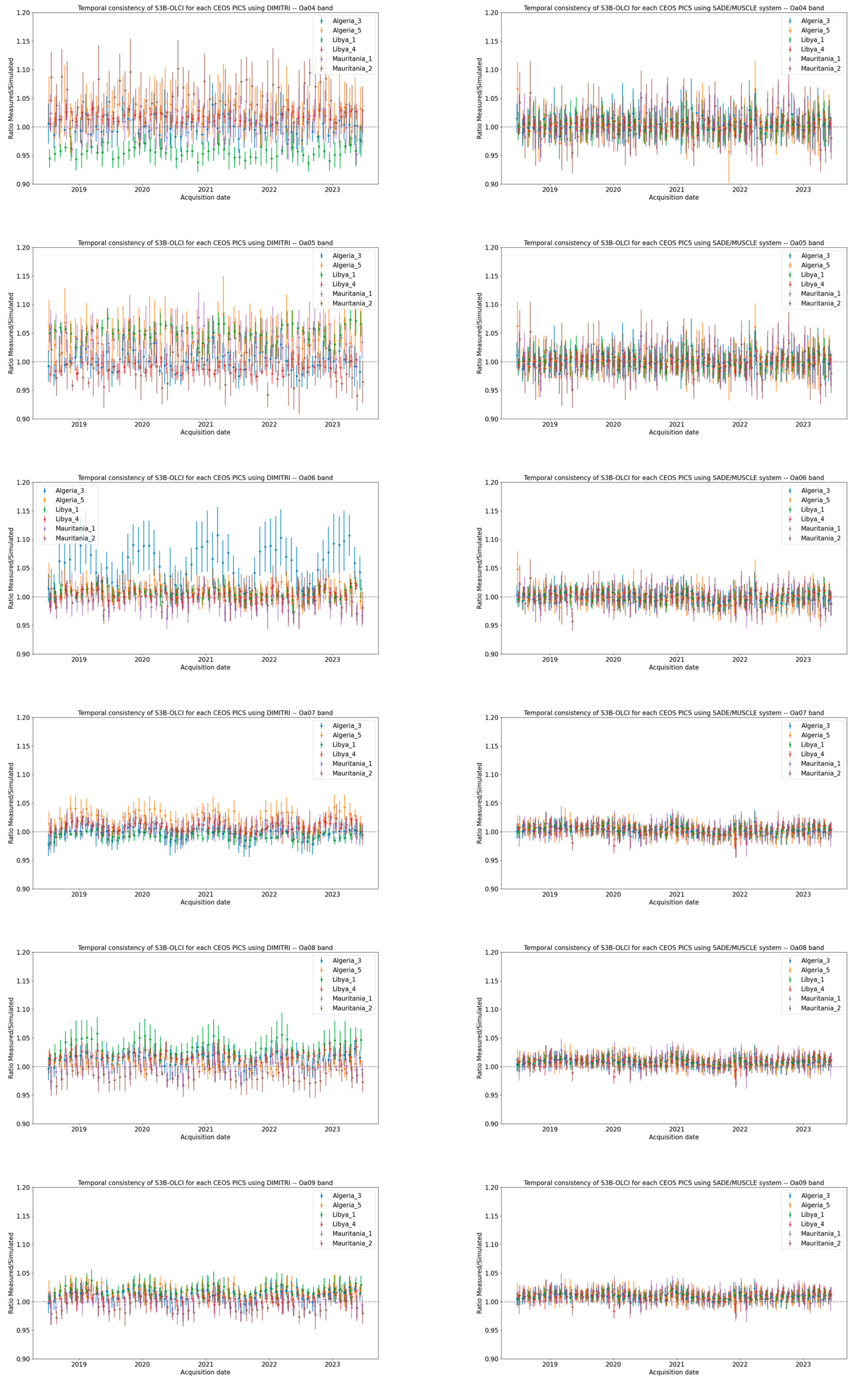
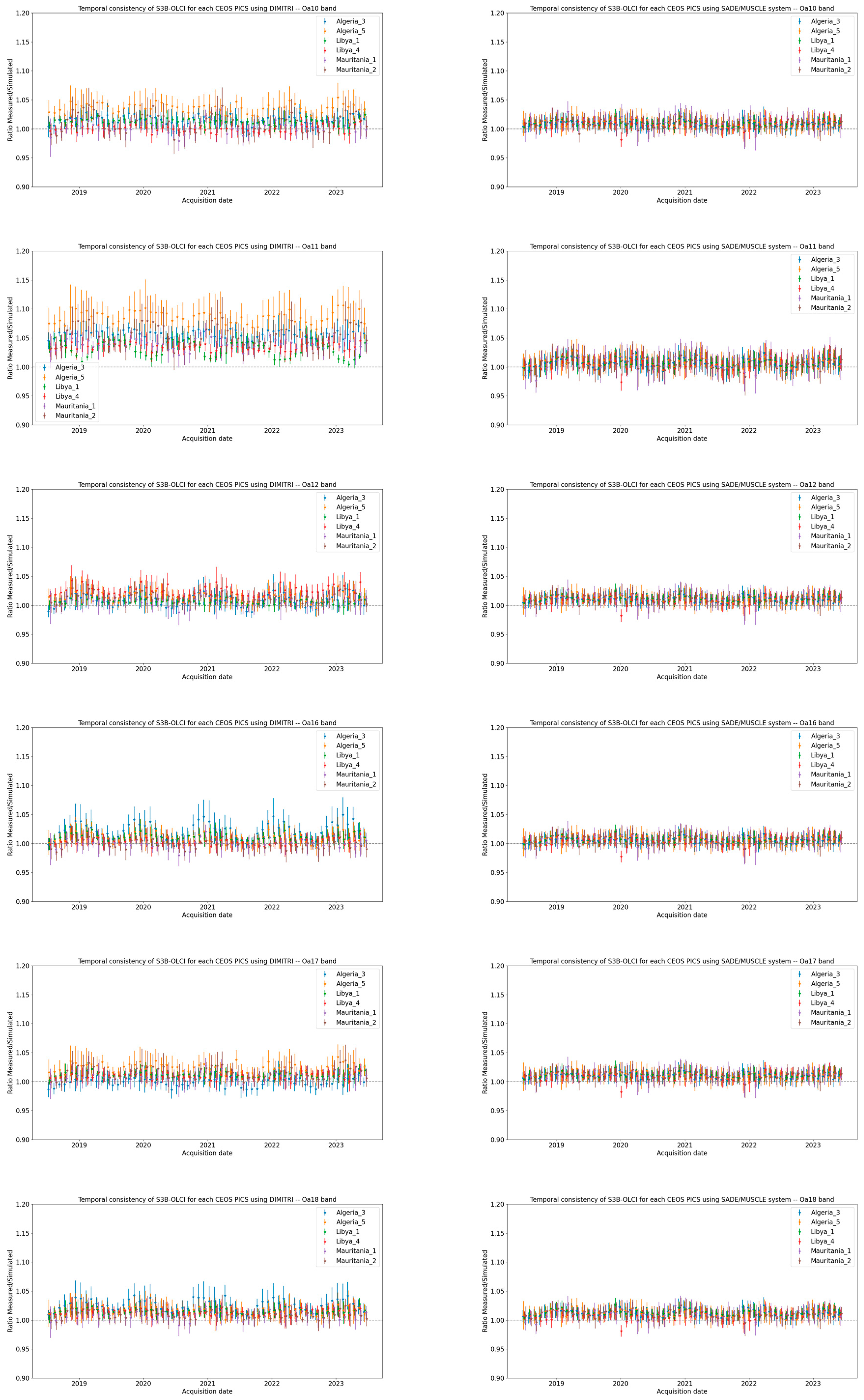
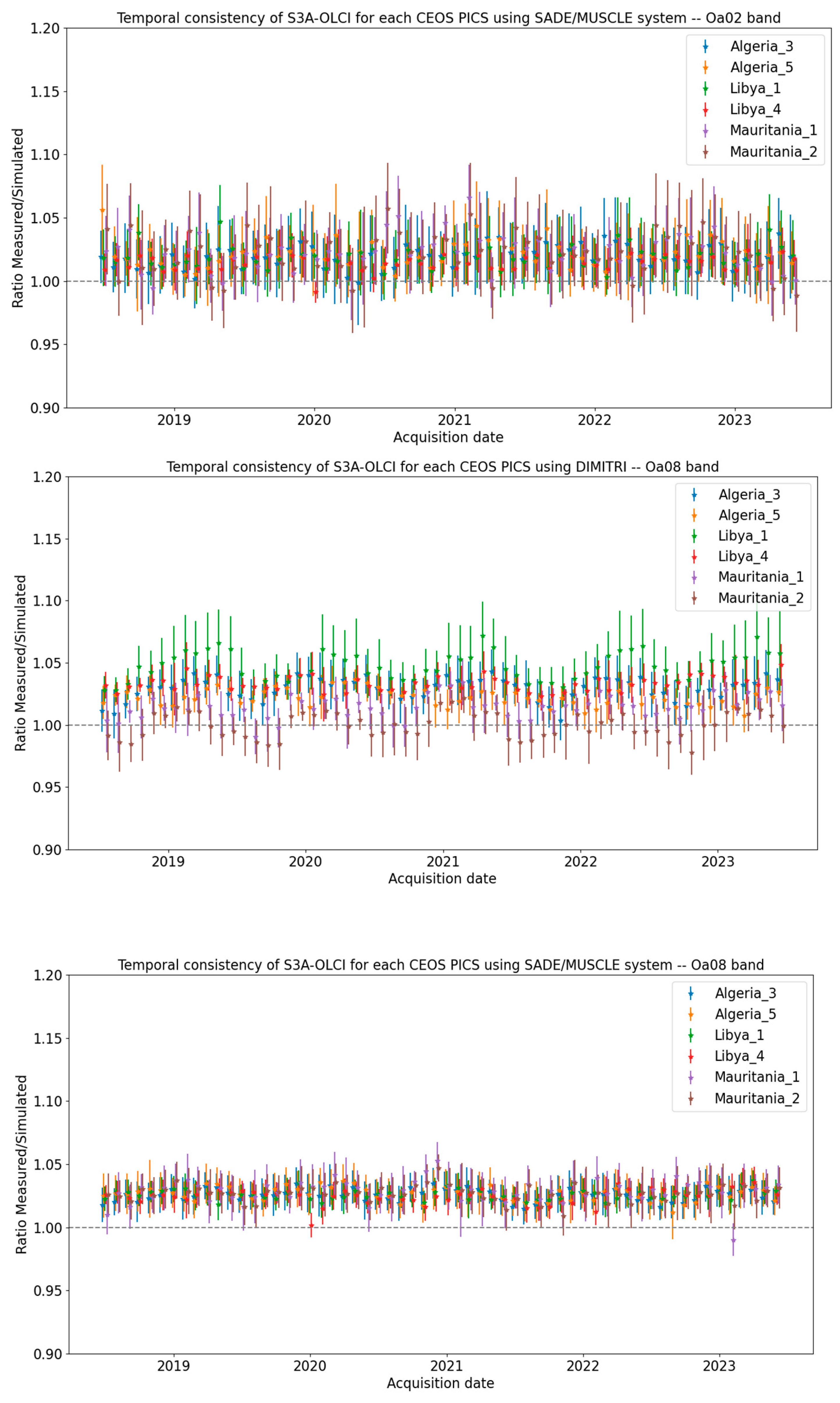
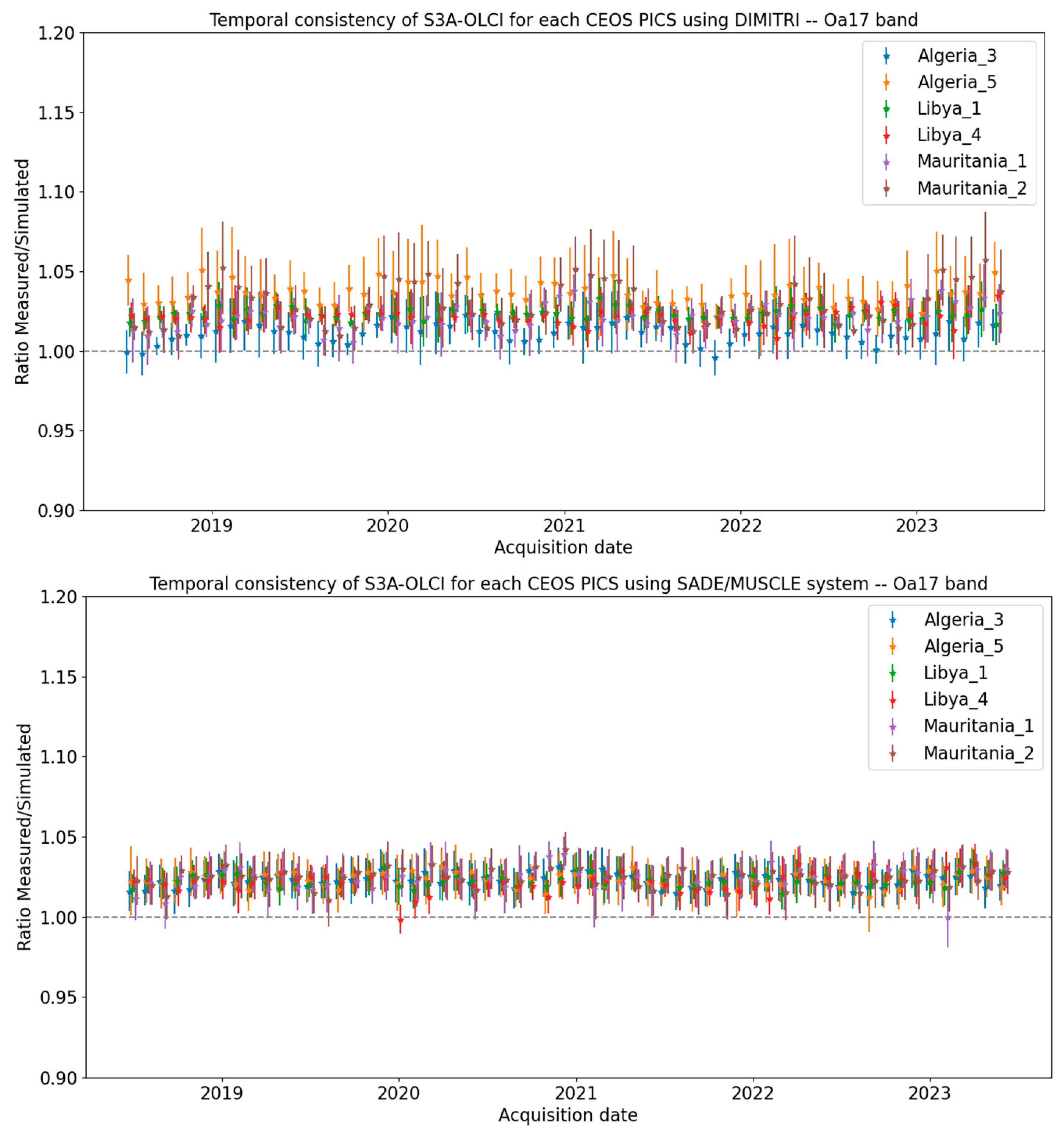
Figure 4 and Figure 5 display the DIMITRI and SADE/MUSCLE monthly time-series of the ratios of TOA-observed over TOA-computed for each site (different colors). The results are consistent over all the used PICS, where both sensors show similar behaviors and good stability—no trend detectable—over the analyzed period. In general, we observe trends of less than 0.08, except bands Oa6 and Oa7 from SADE/MUSCLE which show slightly higher trends of about 0.11 up to 0.15, respectively (Table 4). Despite the good stability over all the time-series, one may observe stronger seasonal variability over DIMITRI results, unlike those of SADE/MUSCLE. Also, differences could be observed over the different sites with band dependency (see Appendix A, Figure A1 and Figure A2).
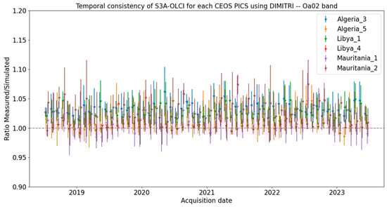
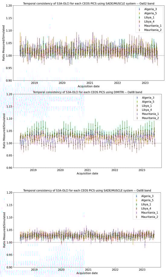

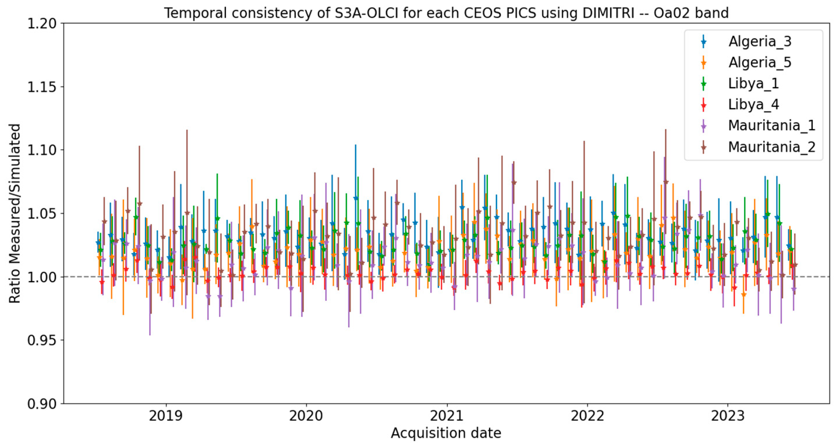
Figure 4.
The time-series of the gain coefficients as ratios (observed/simulated) of the signals from OLCI-A for (top to bottom) bands Oa02, Oa08, and Oa17, respectively, from DIMITRI and Sade/MUSCLE over July 2018–June 2023. The error bars indicate the standard deviation.
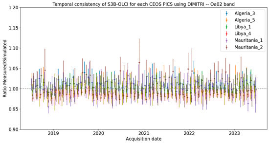
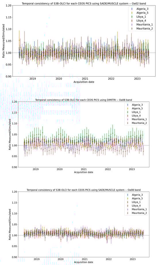
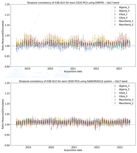
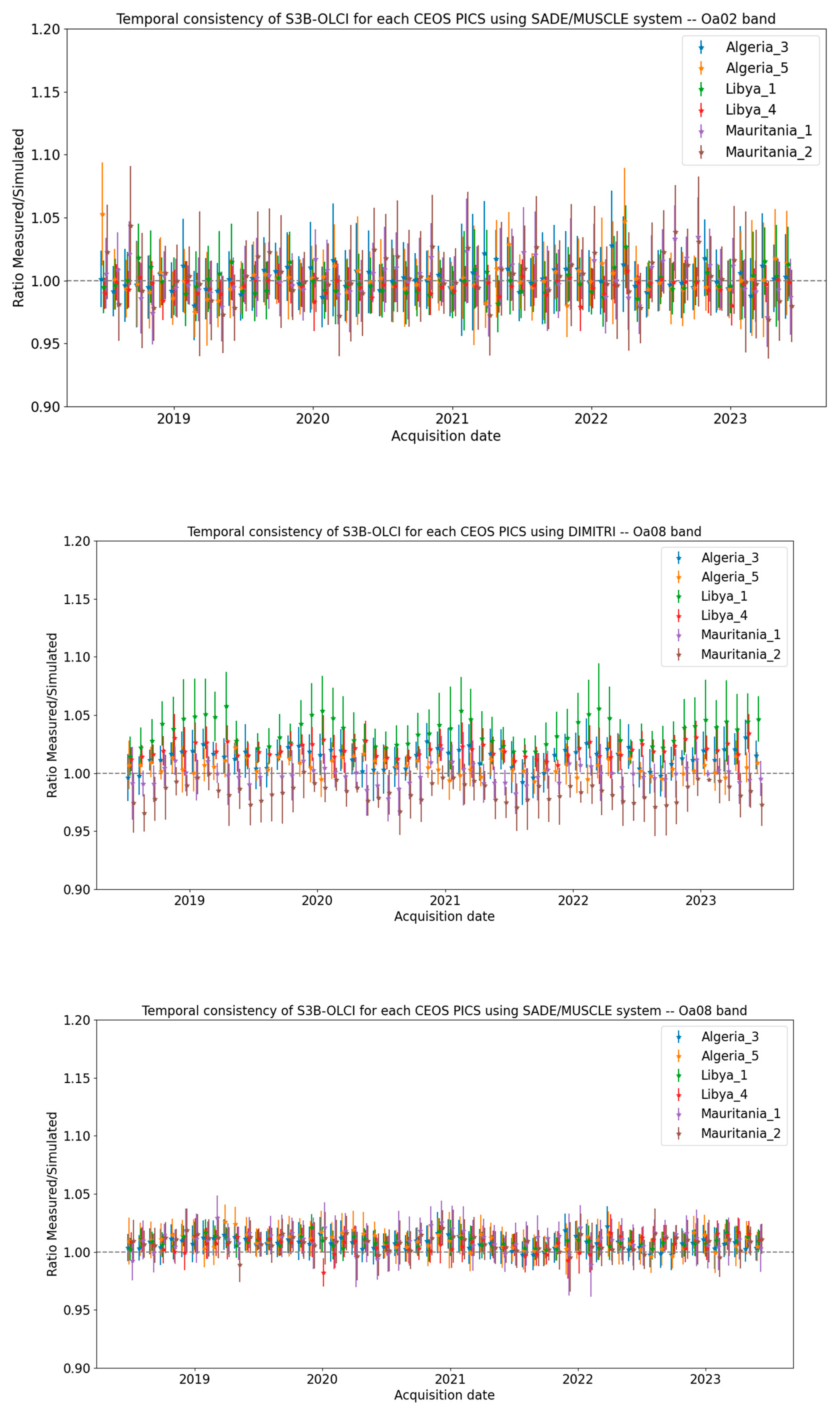
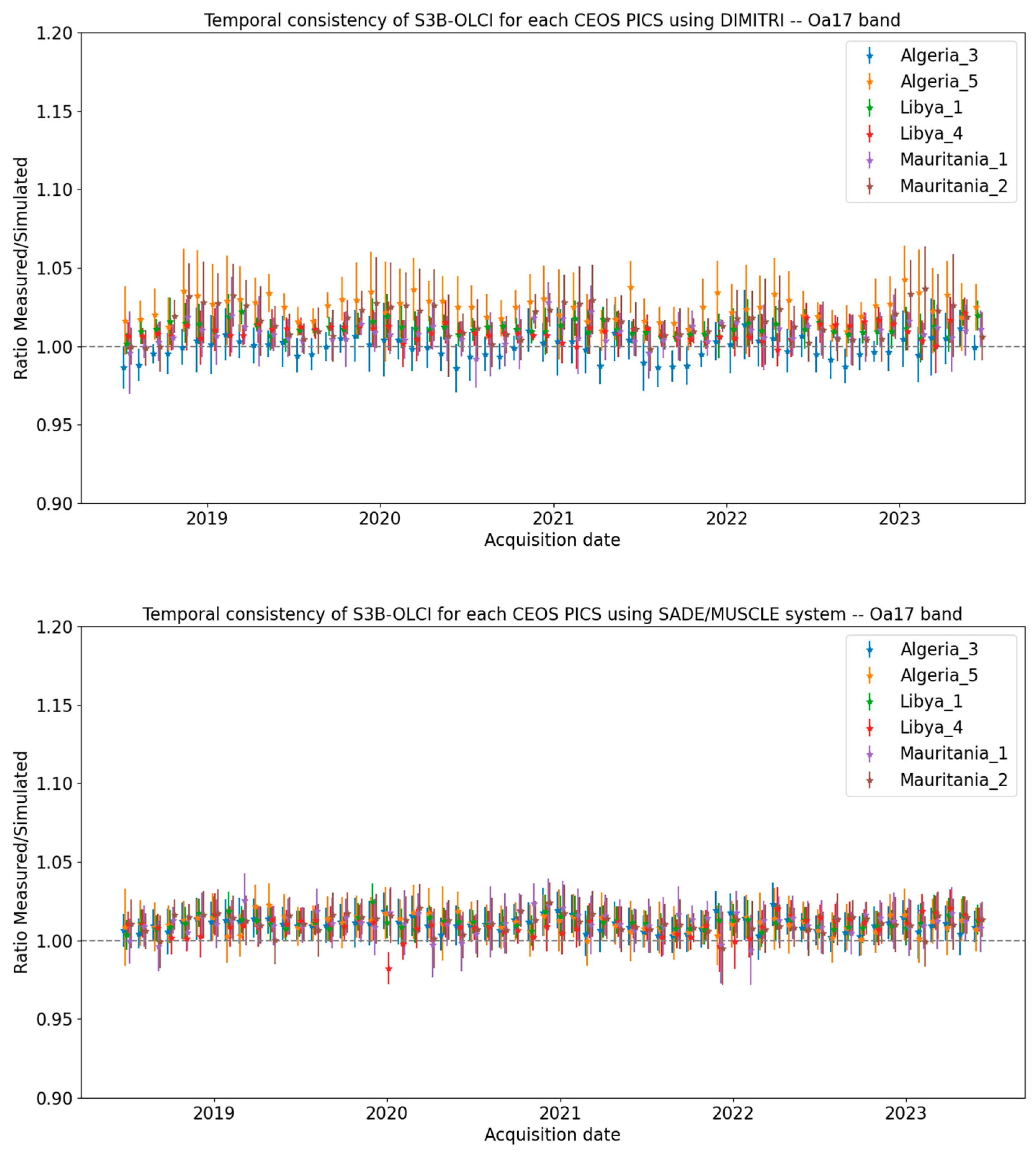
Figure 5.
The time-series of the gain coefficients as ratios (observed/simulated) of the signals from OLCI-B for (top to bottom) bands Oa02, Oa08, and Oa17, respectively, from DIMITRI and Sade/MUSCLE over July 2018–June 2023. The error bars indicate the standard deviation.
Table 4.
Time-series trends of OLCI-A and OLCI-B from DIMITRI and SADE/MUSCLE over desert PICS.
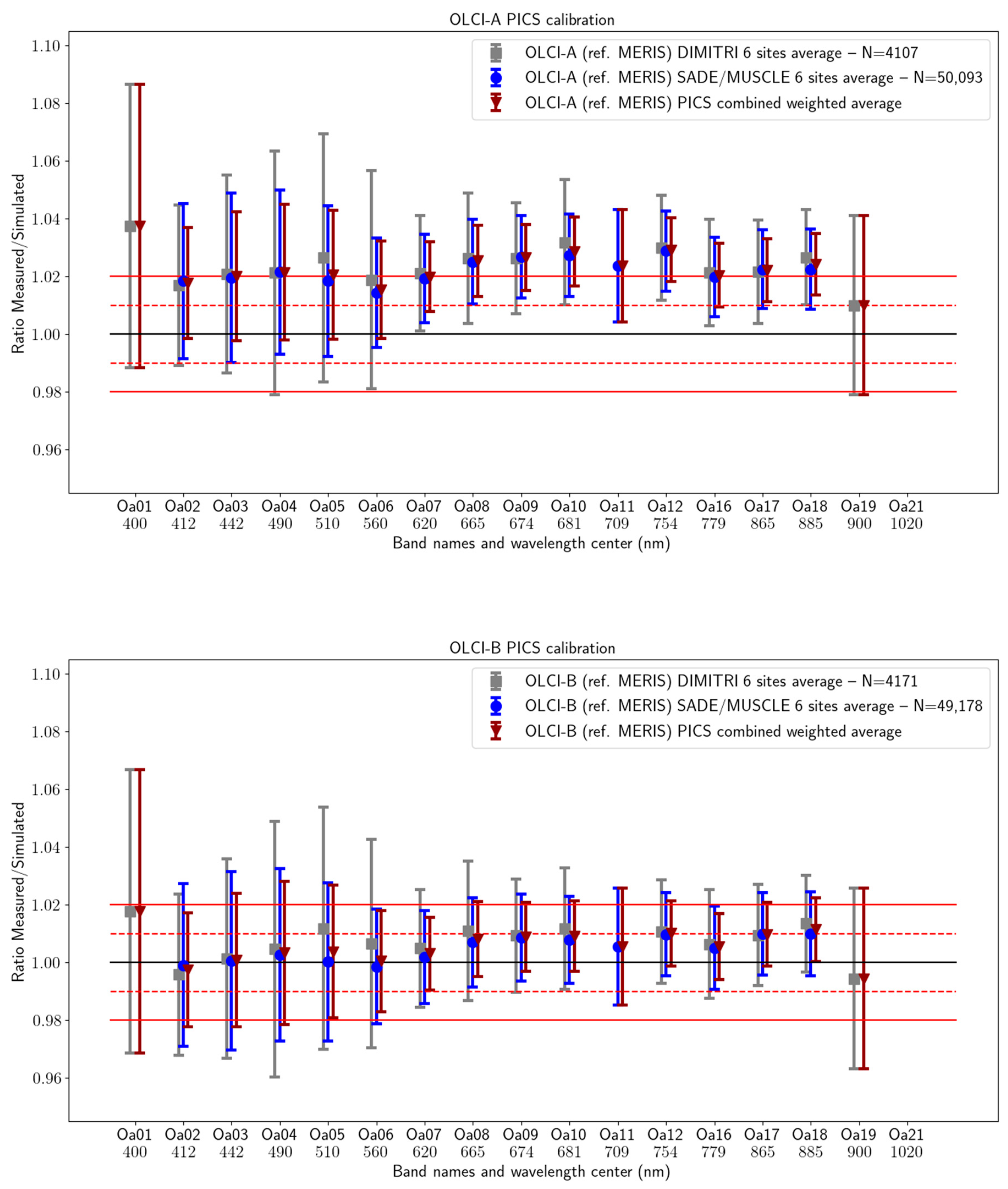
The temporal average of the elementary ratios (observed TOA-reflectance to the TOA-simulated one) over the period of July 2018–June 2023 for OLCI-A shows gain values between 2% and 3% over all the VNIR bands (Figure 6). Improbably, the temporal average of the monthly ratios for OLCI-B shows gain values within 1% (2% is the mission requirement) over the VNIR spectral range except band Oa01 (Figure 6). The spectral bands with significant absorption from water vapor and O2 (Oa11, Oa13, Oa14, Oa15, and Oa20) are excluded. Thus, this shows that there is a 1% to 2% bias between OLCI-A and OLCI-B. One might keep in mind that both software/databases DIMITRI and SADE/MUSCLE use MERIS as a reference sensor (see Section 2.4.1 and Section 2.4.3).
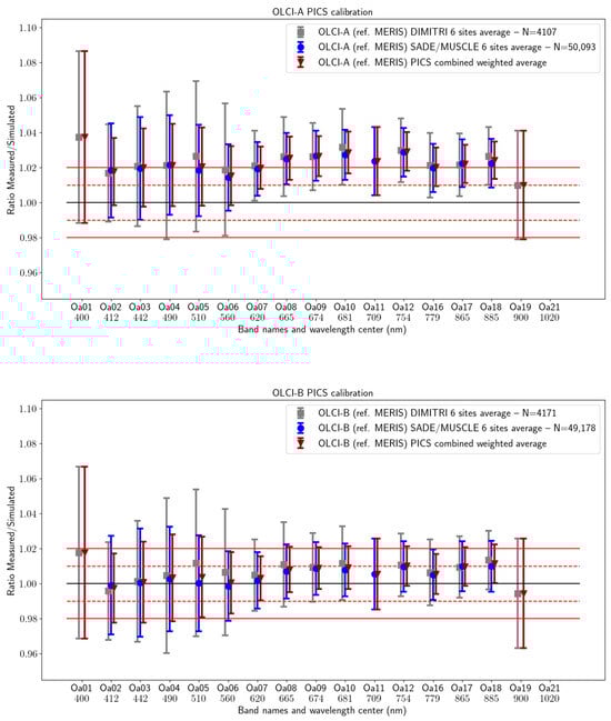
Figure 6.
The estimated gain values from the desert PICS methods for (top) OLCI-A and (bottom) OLCI-B, averaged over the six PICS identified by CEOS and over the period July 2018–June 2023, as a function of wavelength. The dashed and solid red lines indicate the 1% and 2% errors, respectively. The error bars indicate the standard deviation of the results over the six sites.
3.2. Rayleigh Scattering Vicarious Calibration over Ocean Surface Results
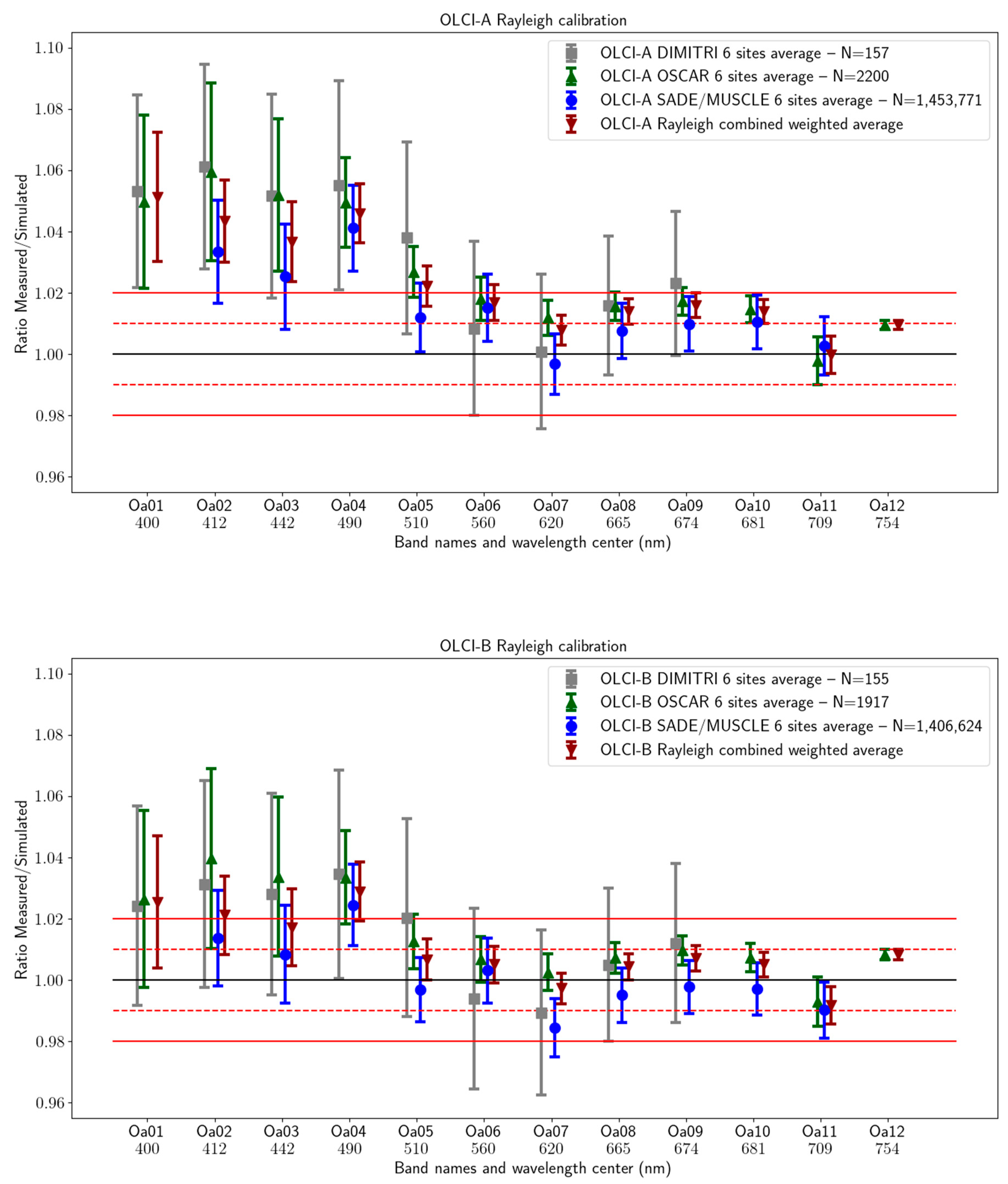
The Rayleigh method was performed by the three software/database kits over the available acquisitions over July 2018–June 2023 from OLCI-A and OLCI-B. The gain coefficients of OLCI-A are consistent over the different sites, while a slight discrepancy could be observed between the northern/southern hemispheres. Bands Oa01–Oa05 display bias values between 5 and 7%, while bands Oa06–Oa12 exhibit biases between 2 and 3% (Figure 7). The gain coefficients of OLCI-A are higher than the OLCI-B ones, where bands Oa01–Oa05 display bias values of about 3–5%, while bands Oa6–Oa12 exhibit biases better than the 2% absolute radiometric accuracy requirement for these bands (Figure 7).
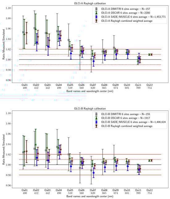
Figure 7.
The estimated gain values from Rayleigh scattering methods for (top) OLCI-A and (bottom) OLCI-B averaged over the six ocean sites (see Section 2.3) during the period July 2018–June 2023 as a function of wavelength. Dashed and solid red lines indicate the 1% and 2% errors, respectively. Error bars indicate the standard deviation of the results.
A bias is observed between OLCI-A and OLCI-B, with OLCI-A being about 2% brighter than OLCI-B in blue bands (i.e., Oa1 to Oa3). This bias seems to decrease to about 1% in green bands and about 0.7% in red bands. Large standard deviation values from DIMITRI could be observed with respect to SADE/MUSCLE and OSCAR ones.
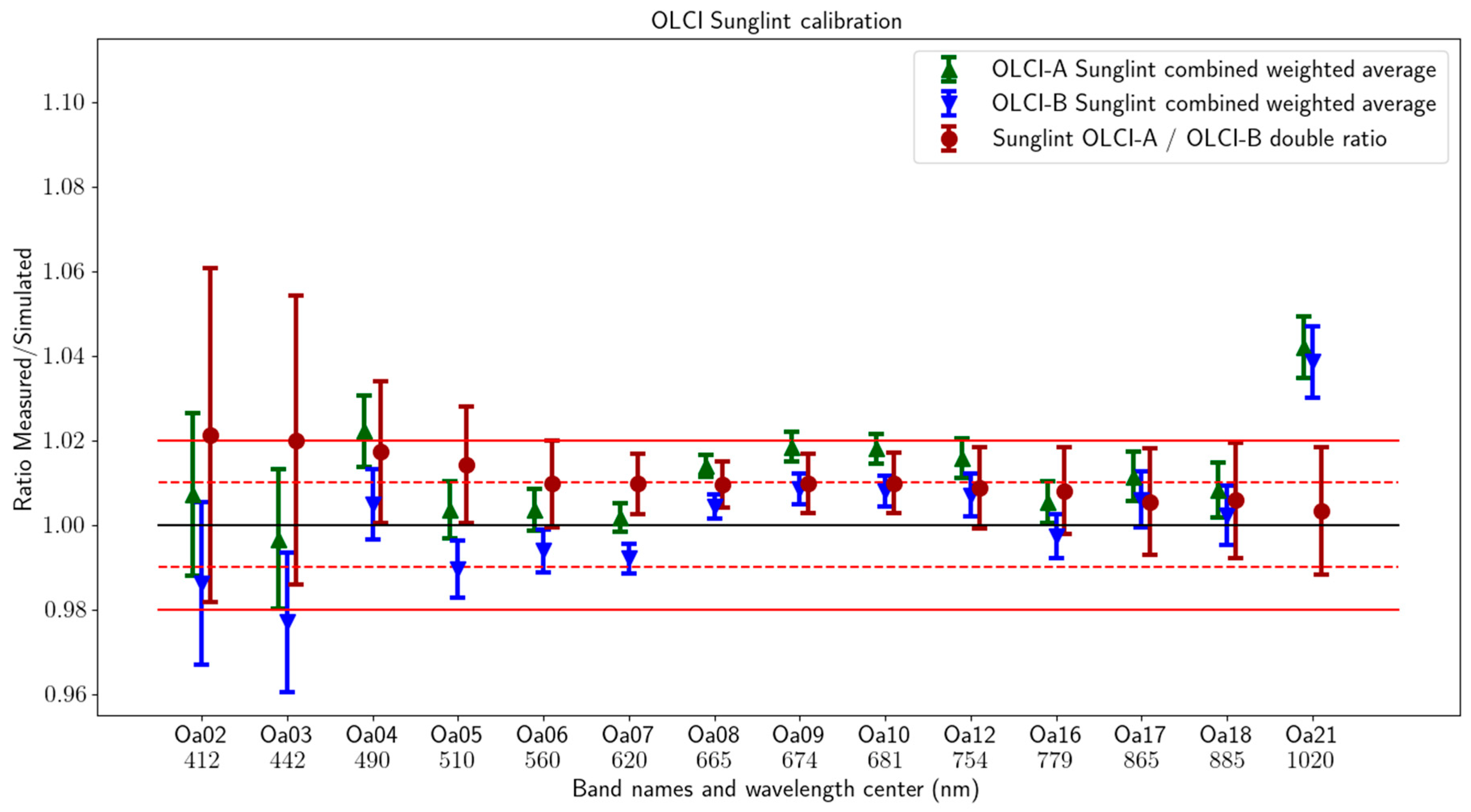
3.3. Inter-Band Vicarious Calibration over Sunglint Results
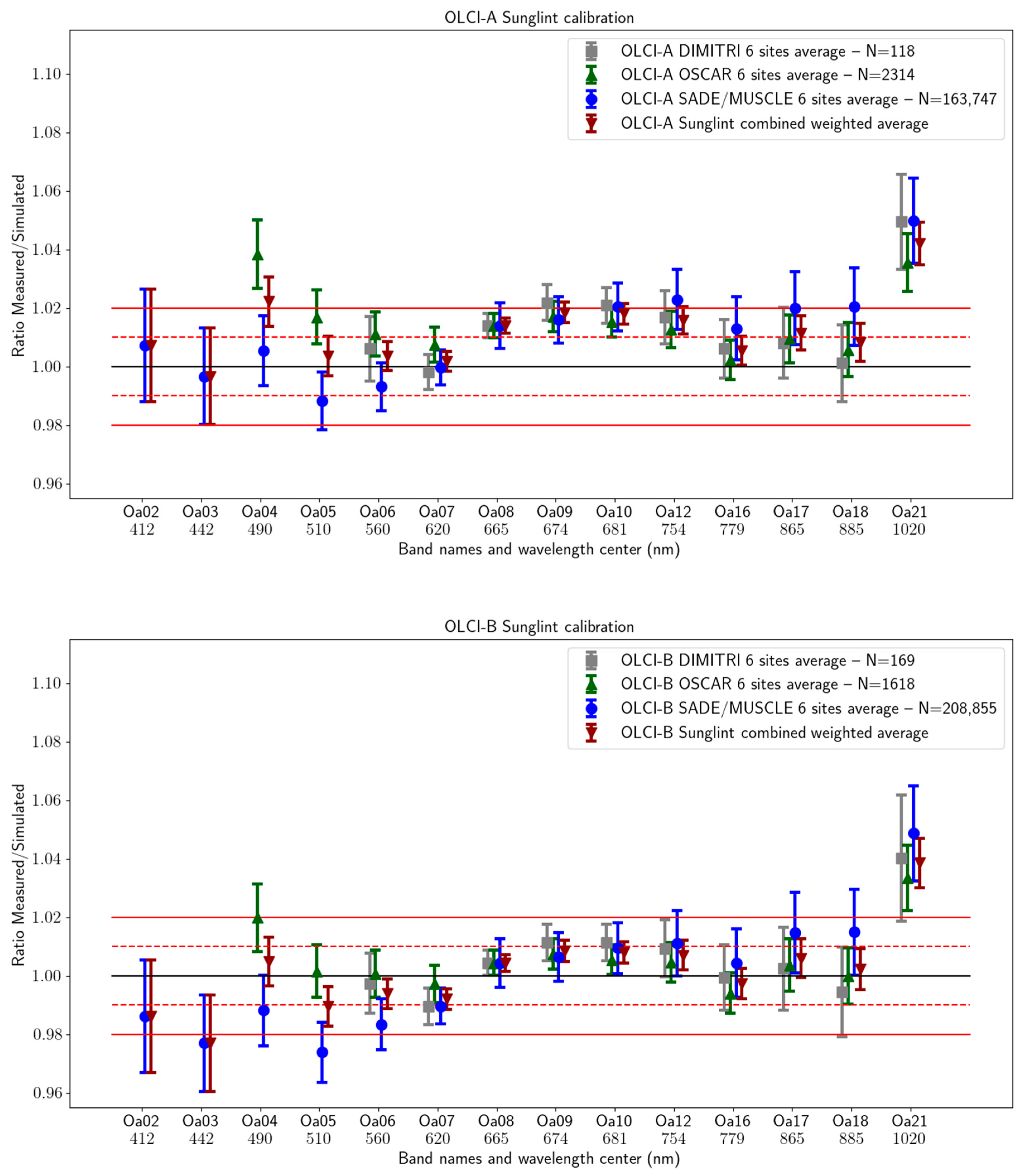
The analysis of glint calibration over the period July 2018–June 2023 shows good consistency between DIMITRI, OSCAR, and SADE/MUSCLE outputs over the reddish-NIR spectral range Oa06–Oa18 for both sensors (Figure 8). The three software/database kits show gain values within the 2% (the mission requirements), while the NIR band Oa21 displays gain values higher than 4% (3% for OSCAR). Glint results from OLCI-A show that the gain values look closer to OLCI-B ones, unlike the observed bias values from Rayleigh scattering and desert PICS methods.
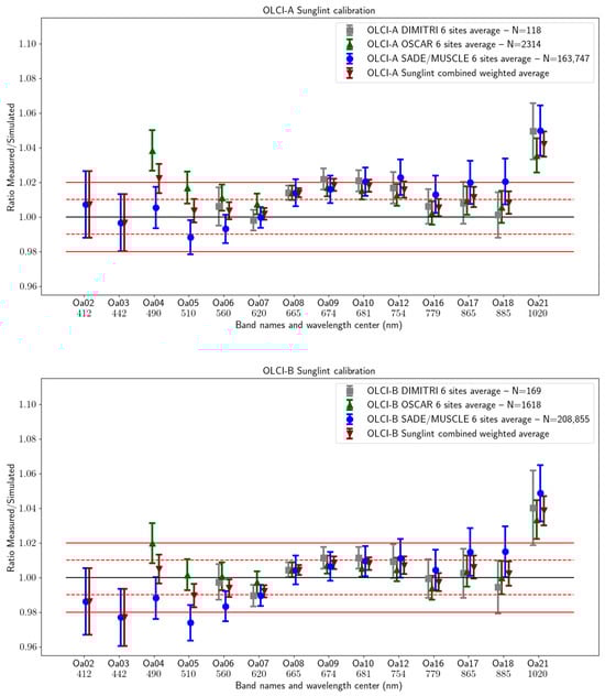
Figure 8.
The estimated gain values from sunglint methods for (top) OLCI-A and (bottom) OLCI-B, averaged over the six ocean sites (see Section 2.3) and over the period July 2018–June 2023, as a function of wavelength. The dashed and solid red lines indicate the 1% and 2% errors, respectively. The error bars indicate the standard deviation of the results.
3.4. OLCI-A and OLCI-B Intercalibration and Result Synthesis
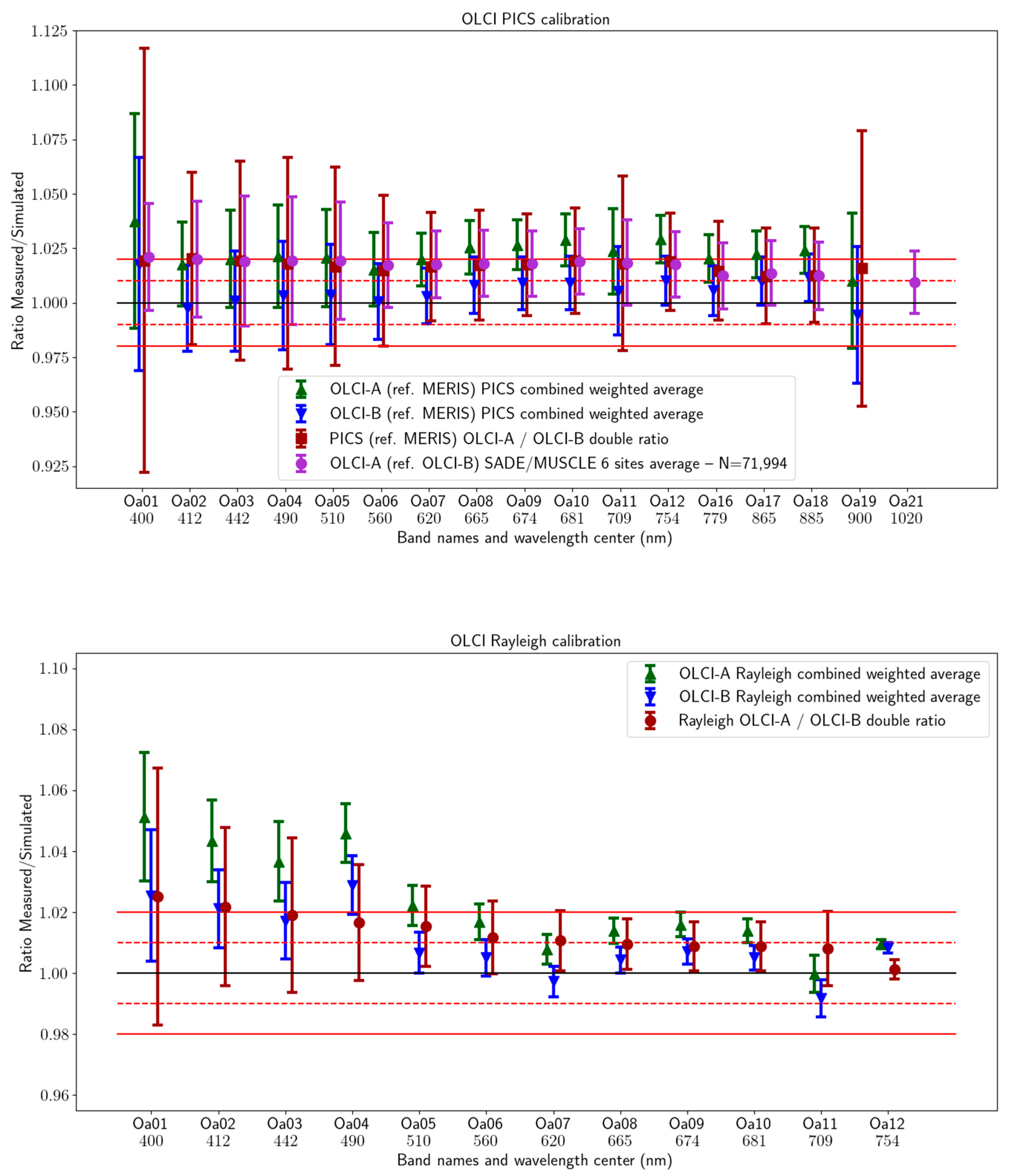
In order to assess the observed biases between OLCI-A and OLCI-B, we used the “double ratios” technique [62]. This involves normalizing the calibration results obtained for a pair of sensors, derived from the same absolute model or reference sensor. Such a technique reduces systematic methodology errors, which leads to more precise evaluation of the performance and discrepancies between the two sensors.
The estimated gain coefficients combined from DIMITRI, OSCAR, and SADE/MUSCLE for OLCI-A vs. OLCI-B over different surface targets (desert and ocean) are displayed on Figure 9 and depicted in Table 5. The combined gain coefficients and standard deviation over desert PICS are computed from the weighted average of the estimated gain coefficients and standard deviations from DIMITRI and SADE/MUSCLE using MERIS as the reference sensor. The weights are the inverse of the squared standard deviation of each dataset. This approach ensures that datasets with lower uncertainties have a higher influence on the results, while those with higher uncertainties contribute less. The combined uncertainties associated with the combined gain coefficients are computed following the GUM law of propagation uncertainties (see Section 5.1 in [62]). We consider that the processes of the gain coefficients estimation are uncorrelated between the three software/database kits since they use different approaches. Then, the double ratios are computed as gain coefficients OLCI-A/OLCI-B (brown squares, Figure 9, top). The gain coefficients of OLCI-A are produced by SADE/MUSCLE again using OLCI-B as a reference sensor instead of MERIS (purple circle, Figure 9, top). These gain coefficients can be compared directly to the former double ratios using MERIS as a reference sensor. Both sets of gain coefficients (brown squares and purple circles) exhibit a very good agreement, better than 0.5%, which is three or four times lower than the PICS methods’ uncertainties. Bands with significant absorption of water vapor and O2 (Oa13, Oa14, and Oa15) were excluded. OLCI-A seems to have higher gain coefficients with respect to OLCI-B. However, the desert PICS methods display a flat spectral shape with 2% discrepancy up to band Oa12 (753.75 nm), while bands Oa16–Oa21 show biases of around 1%. A distinguished pattern of high standard deviation values could be observed over short wavelengths (Oa01–Oa06) and Oa19 (900 nm) (Figure 9, top), while the method’s uncertainty displays nearly the same values of about 3% over the whole spectral range (Table 5).
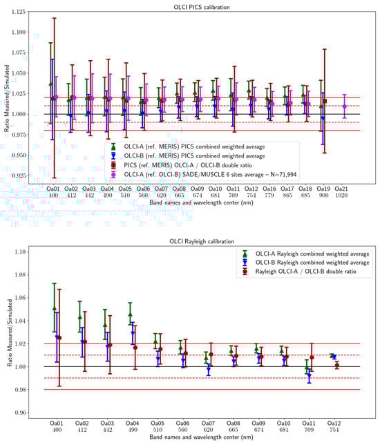
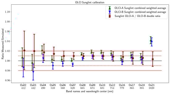
Figure 9.
The estimated gain values weighted and averaged for different groups for OLCI-A and OLCI-B, and the double ratios (OLCI-A/OLCI-B) from the (top) desert PICS method, (middle) Rayleigh scattering method, and (bottom) sunglint method as a function of wavelength. The dashed and solid red lines indicate the 1% and 2% errors, respectively. The error bars indicate the standard deviation of the results.
Table 5.
The double ratios OLCI-A/OLCI-B of the weighted average gain (mean), the combined standard deviation (SD), and the combined total uncertainty (UNC).
The same process was performed on the Rayleigh results from the three software/databases, where the combined weighted averages of the gain coefficients were computed for each sensor, then the double ratios were computed (brown circle, Figure 9, middle). While bands Oa01–Oa04 exhibit discrepancies of about 2%, bands Oa06–Oa11 show biases of about 1%, while band Oa12 (753.75 nm) displays lower bias (close to 0.1%). Also, the Rayleigh results show the same pattern as the desert PICS method, where higher standard deviation values are associated with short wavelengths (Oa01–Oa05), but unlike the desert PICS, the bands Oa01–Oa03 and Oa11–Oa12 show higher uncertainty values than other bands (Table 5).
The results of sunglint method are displayed in Figure 9 (bottom). The double ratios are computed from the weighted average gain as OLCI-A/OLCI-B (brown circle, Figure 9, bottom). The sunglint results display a flat spectral shape with 1% discrepancy over bands Oa05–Oa16, while bands Oa17–Oa21 show biases of about 0.2–0.5% and bands Oa02–Oa04 exhibit higher biases of about 1–2%. In terms of dispersion and uncertainty, sunglint results exhibit nearly the same behavior as Rayleigh results.
4. Discussion
4.1. PICS over Desert Results
We have used the desert PICS method to examine the performance of OLCI-A and OLCI-B L1B radiometry and its temporal variability. Both DIMITRI and SADE/MUSCLE monthly time-series of the ratios of TOA-reflectance (Figure 4) exhibit a 1 to 2% bias between OLCI-A and OLCI-B. Note that both software/databases DIMITRI and SADE/MUSCLE use MERIS as a reference sensor (see Section 2.4.1 and Section 2.4.3). These bias values are confirmed by the SADE/MUSCLE results of the direct cross-calibration over PICS of OLCI-A with OLCI-B in Figure 9. These results are in strong agreement with the results of previous works such as the analysis of the tandem-phase of OLCI-A with OLCI-B in late 2018 [3,4] and the analysis of the post-tandem phase of both sensors [63].
Although both sensors show very good temporal stability over the 5 years (no trend detectable: <0.15%/year worst case; Table 4), a seasonal variability could be observed in DIMITRI results (see Appendix A, Figure A1). The seasonal variability is most likely related to the constant aerosol load used by the DIMITRI PICS method; consequently, larger standard deviation over the results from DIMITRI could be observed (c.f. Figure 6). The seasonal variability of the aerosol load over CEOS PICS has been reported by Bacour et al. [15] (see their Figure 9). In addition, the BDRF model of the site in DIMITRI could introduce such variability due to the slight misfitting of the model parameters (see Section 9.2 in [37]). However, it is most likely that the atmospheric conditions have a higher contribution to these variabilities, particularly on the short wavelength where the standard deviation values exceed the combined uncertainty of the method for these bands (see fourth and fifth columns in Table 5). The high dispersion and uncertainty values of the band Oa01 (400 nm) are most likely related to the use of MERIS as a reference sensor, where its spectral bands do not cover this spectral range. The high dispersion and uncertainty values of the band Oa19 (900 nm) are mainly linked to the impact of the atmospheric conditions and water vapor absorption.
4.2. Rayleigh Scattering over Ocean Results
Although the three software/database kits DIMITRI, OSCAR, and SADE/MUSCLE show similar features, for example, high gain values over the Oa01–Oa05 and lower values for Oa06-Oa12, discrepancies can be observed where SADE/MUSCLE exhibits the lowest gain values. The discrepancy in absolute gain values between the three software/databases may be attributed in part to the different assumptions regarding marine reflectance that were implemented by the three groups: SADE/MUSCLE analysis is grounded on a climatology derived from SEAWIFS, OSCAR uses a climatology from the Copernicus Marine Service (i.e., dataset-oc-glo-chl-olci_a-l4-av_4 km_monthly-rt-v02 products; https://marine.copernicus.eu/sites/default/files/product_improvement_migrated_files/CMEMS_Transition_Document_V3.2.pdf, accessed on 20 March 2025), while DIMITRI employs a marine model following [38] and uses a monthly climatology of chlorophyll concentration from Globcolor project [41] over the period 1998–2012. In addition, each group uses different regions of interest, for example, SADE/MUSCLE results are based on larger sites using macro-pixel averages, while DIMITRI results are based on smaller sites using site averages. This explains the large number of samples in SADE/MUSCLE and the low number in DIMITRI.
The observed differences for the shortest wavelength bands (c.f. Oa01–Oa05; see standard deviation) could be partially attributed to the sensor’s sensitivity to light polarization, given that Rayleigh scattering is highly polarized. However, this is not the only possible explanation. If we consider instrumental effects, discrepancies between the Rayleigh and desert methods could also arise from sensor non-linearity, as Rayleigh calibration is performed over a dark target, whereas desert calibration uses a much brighter reflectance. Another possible cause is the stray light issue, as discussed in [28] on PARASOL/POLDER 443 nm band. Beyond instrumental factors, methodological uncertainties could also contribute to these differences, in particular marine reflectance, atmospheric modeling, chlorophyll variations, etc. This is confirmed by the difference between the standard deviation values and the method uncertainty, where the latter’s values are systematically higher than the former’s values (seventh and eighth columns in Table 5).
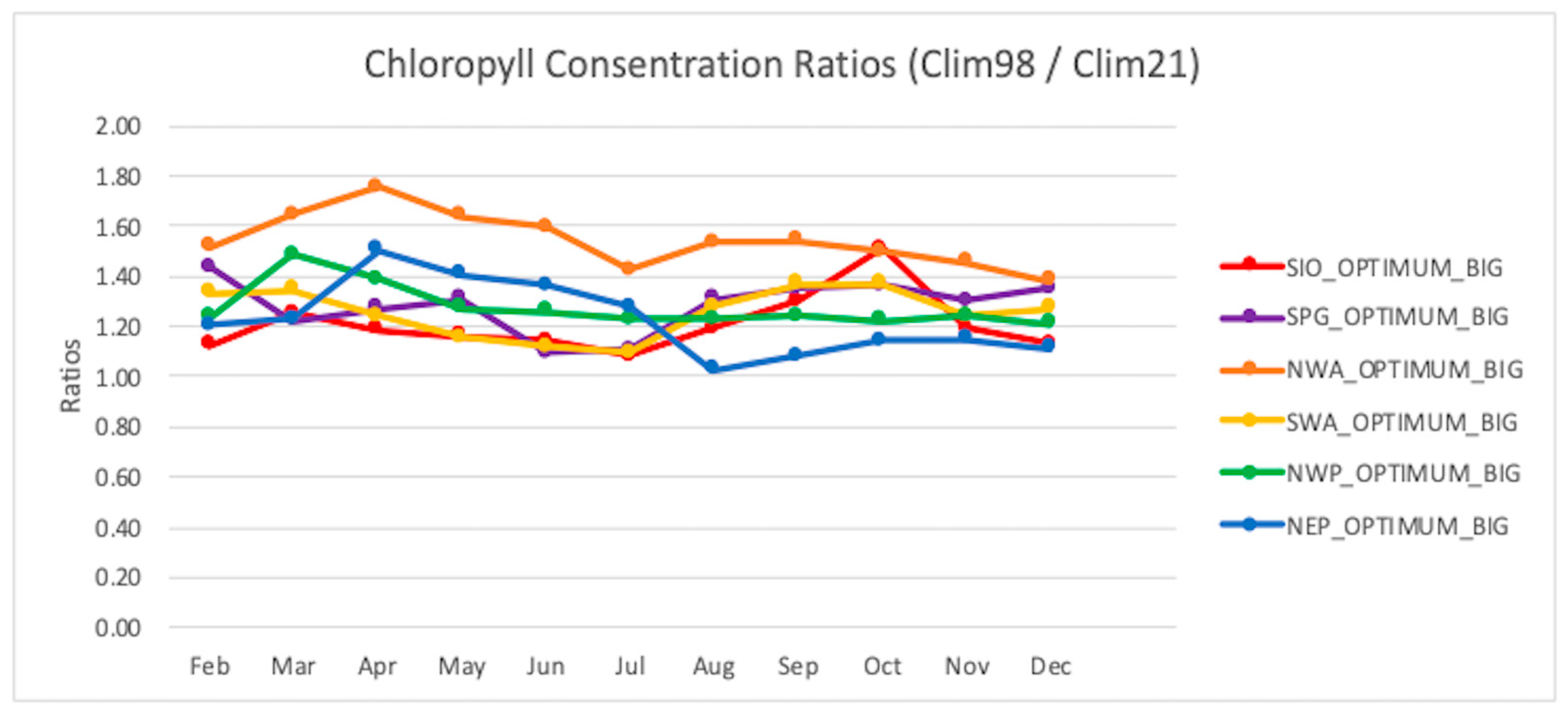
A sensitivity study was undertaken using DIMITRI over the SIO-Optimum CalVal site. The results suggest that the impact of the airmass on the gain coefficients could be up to 1.3% over the short wavelengths (blue-green) and drops down to ~0.5% over the reddish bands. In order to assess the impact of the chlorophyll concentration on Rayleigh gain coefficients, we have performed several sensitivity analyses of the Rayleigh results from DIMITRI employing the same dataset but using two different climatology of chlorophyll concentration. The monthly climatology of chlorophyll concentration from the Globcolor project (Chl1-GSM products; grided by 0.25°) has been extracted over the six CalVal sites over the period 2018–2021 [41,64]. The ratios of the current climatology in DIMITRI (Clim98) to the new climatology (Clim21) show discrepancies of 20%, up to 70%, as a function of the season and the site (Figure 10). The results of the gain coefficient analysis show a discrepancy value up to 2% for blue bands, while it decreases to ~0.1% for red bands (Table 6). These results illustrate the sensitivity of the Rayleigh scattering method to the chlorophyll concentration, particularly over the short wavelength Oa1–Oa4.
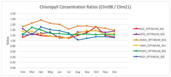
Figure 10.
The ratios of the monthly climatology of the chlorophyll concentration as Clim98/Clim21 (current climatology/recent climatology) per month per site (see Table 2).
Table 6.
The relative difference percent between the average gain coefficients of Rayleigh scattering method from DIMITRI using two different climatologies of chlorophyll concentration (Clim98 and Clim21, see Figure 10).
4.3. Sunglint over Ocean Results
Although sunglint results show the same spectral shape for both sensors and for the three software/database kits, some discrepancies in magnitude are still observed. These discrepancies are most likely related to the different RTMs and ancillary data used by each software. For example, the glint method in DIMITRI is limited over bands >600 nm, while SADE/MUSCLE and OSCAR are applicable over bands >410 nm and >440 nm, respectively. The high dispersion of the results over the blue-green range (see standard deviation in Figure 9) could be explained by the higher sensitivity of these bands to the atmospheric conditions (e.g., air masses) and the chlorophyll concentration in the CalVal site. Although the inter-band uncertainty of the glint method is better than 2%, its total uncertainty is higher than 2% (see 11th column in Table 5) due to the contribution of the reference band uncertainty (e.g., Oa08 from the PICS method for DIMITRI or from the Rayleigh method for OSCAR).
4.4. OLCI-A and OLCI-B Intercalibration Results
If two well-calibrated instruments observe a target under the same illumination and viewing angles, any observed bias between their output signals should be related to the differences in their spectral response functions of the same bands. However, considering that OLCI-A and OLCI-B have similar spectral response functions, and they flew in tandem (~30 s delay) at the beginning of the constellation, this means that both units observed the same target at the same time. Nevertheless, bias of about 1–2% has been observed by Lamquin et al. (2020) [3]; see their Figure 12. The combined results from the three software/database kits are in good agreement with the tandem results, which confirm the very good stability of the sensor calibration and performance. Although the root cause of these biases is still unknown, the estimated differences between the two units based on the combined results over the three methods (PICS, Rayleigh, and sunglint) from the three software/database kits show about 2% over bands Oa01–Oa05 and 1% over the spectral range Oa06–Oa21 (excluding absorption bands; Table 5). However, the estimated differences between both sensors OLCI-A and OLCI-B are still of the same order of magnitude as the combined uncertainty of the different methods used in this analysis (see 13th and 14th columns in Table 5). Hence, the application of different vicarious calibration methods has clearly enhanced the results’ uncertainty. Note that we have considered the uncorrelated assumption of the contributors to our combined uncertainty computing, which adds more uncertainty to the outputs. Also, one must keep in mind that the validation of most of the OLCI spectral bands cannot be achieved by all the vicarious calibration methods (see “N/A” in Table 5).
5. Conclusions and Perspectives
The main objective of the Sentinel-3 OLCI mission is to provide stable time-series of land/ocean images at medium spatial resolution to ensure the continuity of the ENVISAT MERIS legacy. After eight years in orbit and six years in constellation, this objective has been successfully met. Sentinel-3 OLCI time-series are now consistent and comparable with MERIS outcomes, although OLCI-A shows brighter TOA signal than both sensors OLCI-B and MERIS.
In this paper, we have provided an overview of the validation activities and the status of the Sentinel-3/OLCI Level-1 products’ radiometric performances. The results show the good performances of the mission products in terms of radiometry quality, thanks to the robust in-flight calibration strategy. This work has confirmed the 1–2% discrepancy between the two units OLCI-A and OLCI-B, observed during the tandem-phase at the beginning of the constellation life. Although the OLCI-A TOA signal is brighter than the OLCI-B one, the radiometry of the latter is accurate (<2% absolute uncertainty), and both display estimated trends lower than 0.15%/year. The gain coefficients set with their associated uncertainties in Table 5 (12th and 14th columns) could be used to align the TOA reflectance of OLCI-A to OLCI-B. Such vicarious adjustment between the two sensors should lead to more consistent time-series in the future. We believe such alignment is necessary for any future reprocessing of the OLCI-A L1B archive. We recommend another tandem phase with Sentinel-3B at the end of the Sentinel-3A mission life to assess the temporal stability of both missions as well as to check if these biases remain stable. Such a tandem phase could provide more insight on the sensor aging and the sun diffuser degradation.
The sensitivity studies of the Rayleigh scattering method highlighted the impact of chlorophyll concentration hypotheses on the calibration results. Thus, an intercomparison exercise would allow better characterization of the differences between the three implemented methods. In this study, we have not considered very high TOA-reflectance signals such as ice/snow and deep convective cloud targets. Future analysis including such targets would certainly improve these results.
Author Contributions
Conceptualization, B.A., C.D. and S.S.; methodology, B.A., C.D., S.S. and S.A.; software, B.A., C.M., C.D., S.S., S.A. and S.D.; validation, B.A., C.D., S.S. and S.A.; formal analysis and investigation, B.A., C.D., S.S. and S.A.; resources, B.A., C.D., S.S., S.C. and S.D.; data curation, B.A., C.M., C.D., S.S. and S.A.; writing—original draft preparation, B.A., C.D., S.S. and S.A; writing—review and editing, ALL.; visualization, B.A., C.M., C.D., S.S. and S.A; supervision, L.B.; project administration, L.B. and S.C.; funding acquisition, B.A., C.D., S.S., S.C. and S.D. All authors have read and agreed to the published version of the manuscript.
Funding
This research and the APC were funded by the European Space Agency via the framework of Copernicus Sentinel Optical Mission Performance Cluster under the contract number 4000136252/21/I-BG, and via the framework of DIMITRI-QA4EO project under the contract number 4000114544/15/I-SBo.
Data Availability Statement
The Sentinel-3/OLCI Level-1B products are available through the Copernicus Data Space Ecosystem (CDSE) portal: https://dataspace.copernicus.eu/ (accessed on 20 March 2025); the extracted datasets by S3ETRAC and DIMITRI are archived at the Copernicus Optical Missions Performance Cluster (OPT-MPC) and could be made available upon request.
Acknowledgments
The authors greatly acknowledge the five anonymous reviewers for their insightful comments, which significantly improved the quality of the manuscript. Experts contributing to the Optical Mission Performance Cluster are acknowledged for the useful comments which helped improve this manuscript. The authors would like to acknowledge the administrative support by J. Bruniquel (OPT-MPC service manager) and the technical support of all the Sentinel-3 operators at OPT-MPC. BA would like to thank A. Deru for the fruitful discussion on the uncertainty computing.
Conflicts of Interest
Authors Bahjat Alhammoud, Ludovic Bourg and Sebastien Clerc are employed by the company ACRI-ST. Bahjat Alhammoud (formerly) and Cameron Mackenzie were employed by the company ARGANS Ltd. The remaining authors declare that the research was conducted in the absence of any commercial or financial relationships that could be construed as a potential conflict of interest.
Appendix A
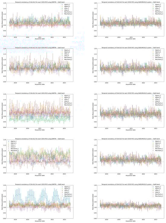
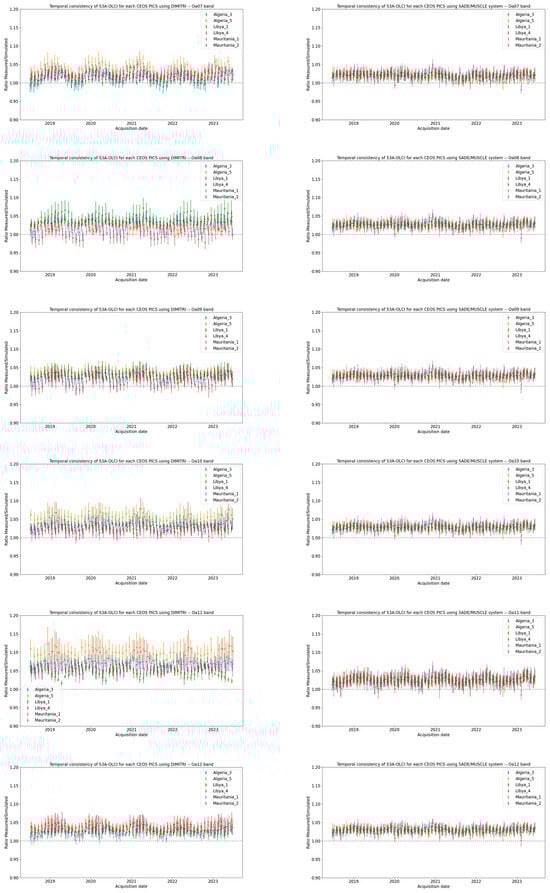
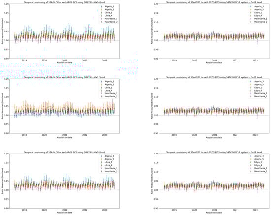
Figure A1.
Time-series of gain coefficients as ratios (observed/simulated) of signals from OLCI-A for bands Oa02–Oa18 (Oa13–Oa15 excluded) from (left) DIMITRI and (right) Sade/MUSCLE over July 2018–June 2023. Error bars indicate standard deviation.
Figure A1.
Time-series of gain coefficients as ratios (observed/simulated) of signals from OLCI-A for bands Oa02–Oa18 (Oa13–Oa15 excluded) from (left) DIMITRI and (right) Sade/MUSCLE over July 2018–June 2023. Error bars indicate standard deviation.
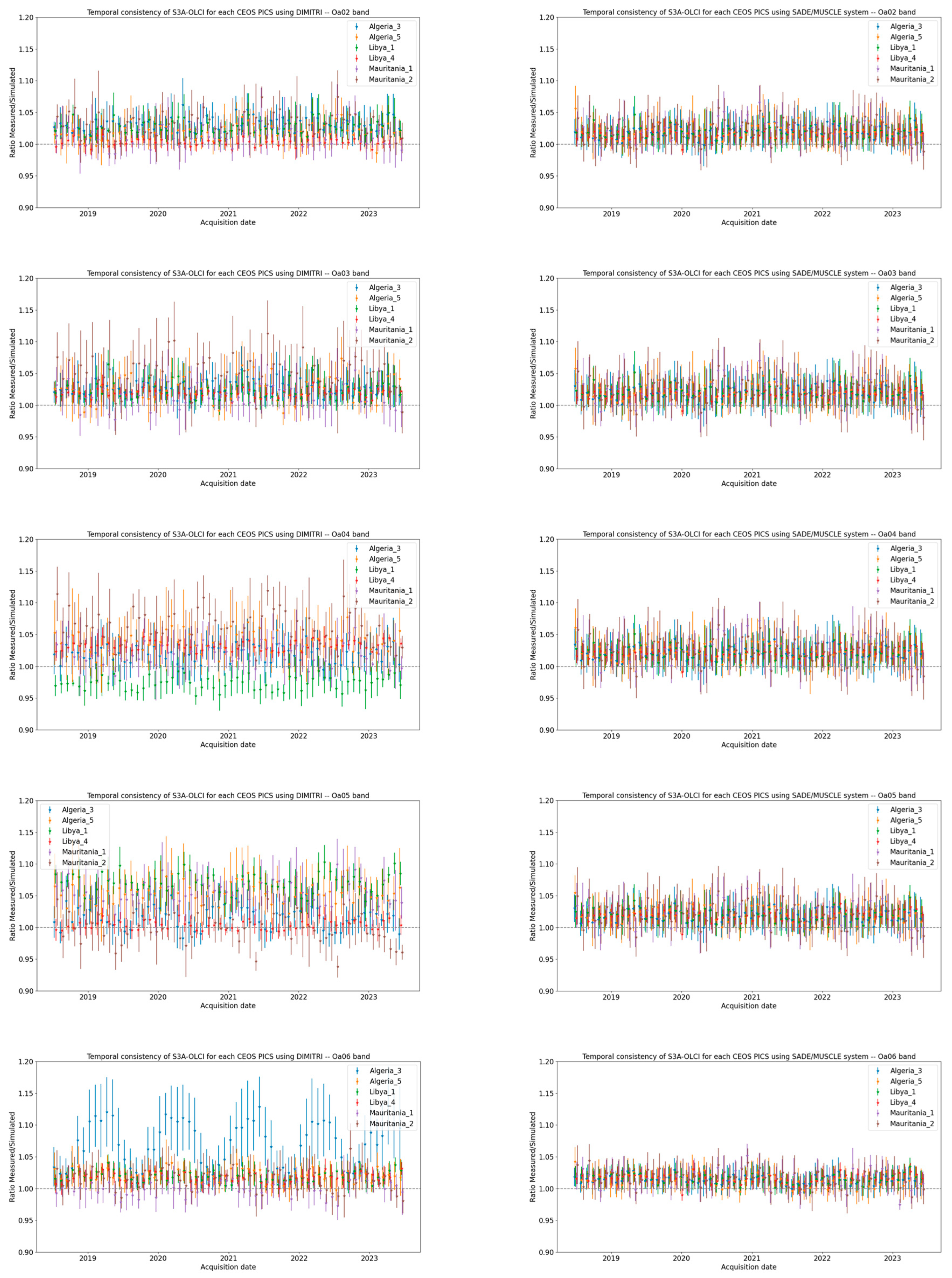
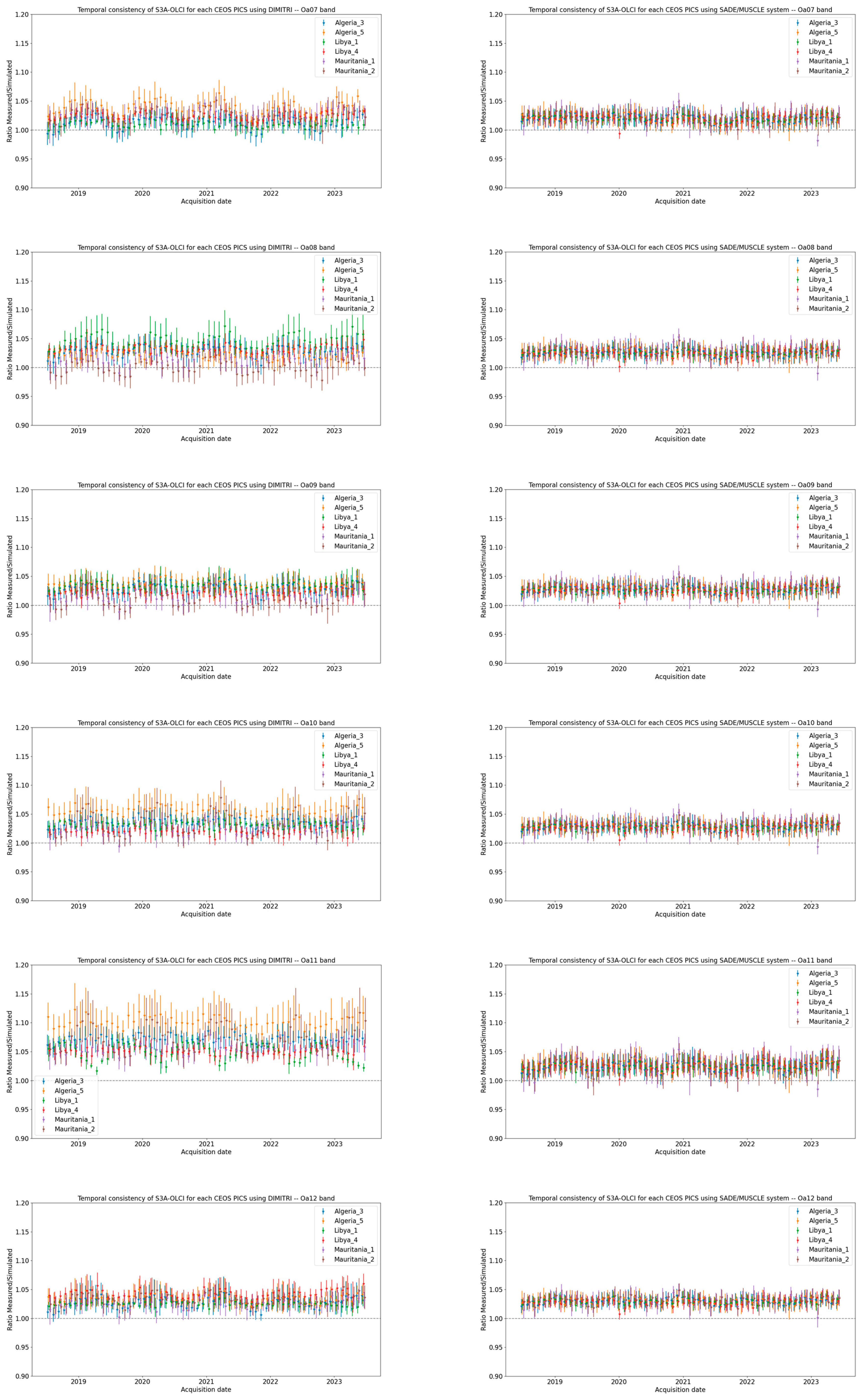
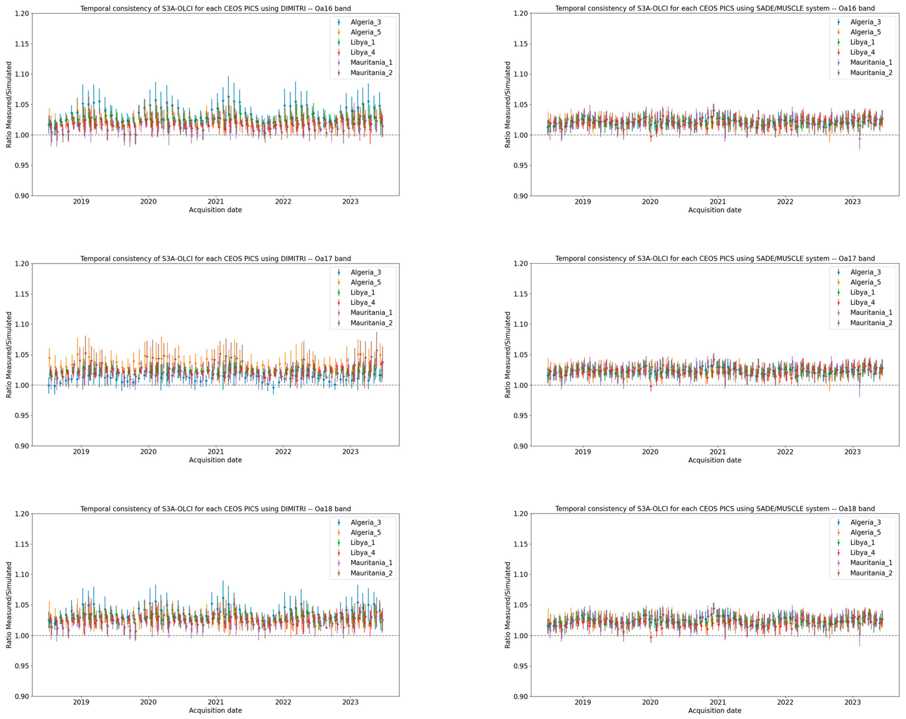
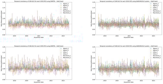
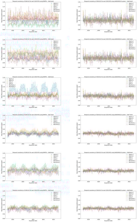
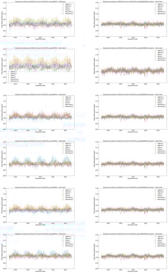
Figure A2.
Time-series of gain coefficients as ratios (observed/simulated) of signals from OLCI-B for bands Oa02–Oa18 (Oa13–Oa15 excluded) from (left) DIMITRI and (right) Sade/MUSCLE over July 2018–June 2023. Error bars indicate standard deviation.
Figure A2.
Time-series of gain coefficients as ratios (observed/simulated) of signals from OLCI-B for bands Oa02–Oa18 (Oa13–Oa15 excluded) from (left) DIMITRI and (right) Sade/MUSCLE over July 2018–June 2023. Error bars indicate standard deviation.

References
- Donlon, C.; Berruti, B.; Buongiorno, A.; Ferreira, M.-H.; Féménias, P.; Frerick, J.; Goryl, P.; Klein, U.; Laur, H.; Mavrocordatos, C.; et al. The Global Monitoring for Environment and Security (GMES) Sentinel-3 Mission. Remote Sens. Environ. 2012, 120, 37–57. [Google Scholar] [CrossRef]
- Lamquin, N.; Bourg, L.; Clerc, S.; Donlon, C. OLCI A/B Tandem Phase Analysis, Part 3: Post-Tandem Monitoring of Cross-Calibration from Statistics of Deep Convective Clouds Observations. Remote Sens. 2020, 12, 3105. [Google Scholar] [CrossRef]
- Lamquin, N.; Clerc, S.; Bourg, L.; Donlon, C. OLCI A/B Tandem Phase Analysis, Part 1: Level 1 Homogenisation and Harmonisation. Remote Sens. 2020, 12, 1804. [Google Scholar] [CrossRef]
- Clerc, S.; Donlon, C.; Borde, F.; Lamquin, N.; Hunt, S.E.; Smith, D.; McMillan, M.; Mittaz, J.; Woolliams, E.; Hammond, M.; et al. Benefits and Lessons Learned from the Sentinel-3 Tandem Phase. Remote Sens. 2020, 12, 2668. [Google Scholar] [CrossRef]
- Lamquin, N.; Woolliams, E.; Bruniquel, V.; Gascon, F.; Gorroño, J.; Govaerts, Y.; Leroy, V.; Lonjou, V.; Alhammoud, B.; Barsi, J.A.; et al. An Inter-Comparison Exercise of Sentinel-2 Radiometric Validations Assessed by Independent Expert Groups. Remote Sens. Environ. 2019, 233, 111369. [Google Scholar] [CrossRef]
- Bourg, L.; Bruniquel, J.; Henocq, C.; Morris, H.; Dash, J.; Preusker, R.; Dransfeld, S. Copernicus Sentinel-3 OLCI Land User Handbook; European Space Agen: Paris, France; European Commission: Brussels, Belgium, 2023. [Google Scholar]
- Bourg, L.; Pflug, B.; Bachmann, M.; Malle, M.; Gobron, N. Copernicus Cal/Val Solution—D1.1—Optical Missions Cal/Val Requirements; European Commission: Brussels, Belgium, 2021. [Google Scholar]
- Fougnie, B. S3ETRAC Preprocessing and Extraction Specification of the Sentinel-3 Extraction Tool for Radiometric Analysis and Calibration (ATBD) 2014; European Space Agen: Paris, France, 2014. [Google Scholar]
- Holben, B.N.; Kaufman, Y.J.; Kendall, J.D. NOAA-11 AVHRR Visible and near-IR Inflight Calibration. Int. J. Remote Sens. 1990, 11, 1511–1519. [Google Scholar] [CrossRef]
- Govaerts, Y.M.; Clerici, M. Evaluation of Radiative Transfer Simulations over Bright Desert Calibration Sites. IEEE Trans. Geosci. Remote Sens. 2004, 42, 176–187. [Google Scholar] [CrossRef]
- Slater, P.N.; Biggar, S.F.; Holm, R.G.; Jackson, R.D.; Mao, Y.; Moran, M.S.; Palmer, J.M.; Yuan, B. Reflectance- and Radiance-Based Methods for the in-Flight Absolute Calibration of Multispectral Sensors. Remote Sens. Environ. 1987, 22, 11–37. [Google Scholar] [CrossRef]
- Lacherade, S.; Fougnie, B.; Henry, P.; Gamet, P. Cross Calibration Over Desert Sites: Description, Methodology, and Operational Implementation. IEEE Trans. Geosci. Remote Sens. 2013, 51, 1098–1113. [Google Scholar] [CrossRef]
- Bouvet, M. Radiometric Comparison of Multispectral Imagers over a Pseudo-Invariant Calibration Site Using a Reference Radiometric Model. Remote Sens. Environ. 2014, 140, 141–154. [Google Scholar] [CrossRef]
- Cosnefroy, H.; Leroy, M.; Briottet, X. Selection and Characterization of Saharan and Arabian Desert Sites for the Calibration of Optical Satellite Sensors. Remote Sens. Environ. 1996, 58, 101–114. [Google Scholar] [CrossRef]
- Bacour, C.; Briottet, X.; Bréon, F.-M.; Viallefont-Robinet, F.; Bouvet, M. Revisiting Pseudo Invariant Calibration Sites (PICS) Over Sand Deserts for Vicarious Calibration of Optical Imagers at 20 Km and 100 Km Scales. Remote Sens. 2019, 11, 1166. [Google Scholar] [CrossRef]
- Shrestha, M.; Leigh, L.; Helder, D. Classification of North Africa for Use as an Extended Pseudo Invariant Calibration Sites (EPICS) for Radiometric Calibration and Stability Monitoring of Optical Satellite Sensors. Remote Sens. 2019, 11, 875. [Google Scholar] [CrossRef]
- Kabir, S.; Leigh, L.; Helder, D. Vicarious Methodologies to Assess and Improve the Quality of the Optical Remote Sensing Images: A Critical Review. Remote Sens. 2020, 12, 4029. [Google Scholar] [CrossRef]
- Gordon, H.R.; Wang, M. Retrieval of Water-Leaving Radiance and Aerosol Optical Thickness over the Oceans with SeaWiFS: A Preliminary Algorithm. Appl. Opt. 1994, 33, 443–452. [Google Scholar] [CrossRef] [PubMed]
- Morel, A. Optical Modeling of the Upper Ocean in Relation to Its Biogenous Matter Content (Case I Waters). J. Geophys. Res. Oceans 1988, 93, 10749–10768. [Google Scholar] [CrossRef]
- Morel, A.; Prieur, L. Analysis of Variations in Ocean Color. Limnol. Oceanogr. 1977, 22, 709–722. [Google Scholar] [CrossRef]
- Shettle, E.; Fenn, R. Models for the Aerosols of the Lower Atmosphere and the Effects of Humidity Variations on Their Optical Properties. Environ. Res. Pap. 1979, 676, 94. [Google Scholar]
- VERMOTE, E.; SANTER, R.; DESCHAMPS, P.Y.; HERMAN, M. In-Flight Calibration of Large Field of View Sensors at Short Wavelengths Using Rayleigh Scattering. Int. J. Remote Sens. 1992, 13, 3409–3429. [Google Scholar] [CrossRef]
- VERMOTE, E.; KAUFMAN, Y.J. Absolute Calibration of AVHRR Visible and Near-Infrared Channels Using Ocean and Cloud Views. Int. J. Remote Sens. 1995, 16, 2317–2340. [Google Scholar] [CrossRef]
- Moulin, F.; Bernard, D.; Amiranoff, F. Photon-Photon Elastic Scattering in the Visible Domain. Z. Für Phys. C Part. Fields 1996, 72, 607–611. [Google Scholar] [CrossRef]
- Hagolle, O.; Cabot, F. Absolute Calibration of MERIS Using Natural Targets. In Proceedings of the Working Meeting on MERIS and AATSR Calibration and Geophysical Validation, Frascati, Italy, 20–24 October 2003; pp. 20–24. [Google Scholar]
- Meygret, A.; Briottet, X.; Henry, P.J.; Hagolle, O. Calibration of SPOT4 HRVIR and Vegetation Cameras over Rayleigh Scattering. In Proceedings of the Earth Observing Systems V, San Diego, CA, USA, 22 July–4 August 2000; Barnes, W.L., Ed.; SPIE: Bellingham, WA, USA, 2000; p. 302. [Google Scholar]
- Bruniquel, V.; e Fontanilles, G.; Bourg, L.; Fougnie, B.; Henry, P. Absolute Calibration of SeaWiFS Using Rayleigh Scattering. In Proceedings of the International Ocean Colour Science Meeting, Baltimore, MD, USA, 13–15 May 2013; Volume 43. [Google Scholar]
- Fougnie, B.; Desjardins, C.; Besson, B.; Bruniquel, V.; Meskini, N.; Nieke, J.; Bouvet, M. Results from the Radiometric Validation of Sentinel-3 Optical Sensors Using Natural Targets. In Proceedings of the Earth Observing Systems XXI, San Diego, CA, USA, 28 August–1 September 2016; Butler, J.J., Xiong, X., Gu, X., Eds.; SPIE: Bellingham, WA, USA, 2016; p. 99720O. [Google Scholar]
- Fougnie, B.; Bracco, G.; Lafrance, B.; Ruffel, C.; Hagolle, O.; Tinel, C. PARASOL In-Flight Calibration and Performance. Appl. Opt. 2007, 46, 5435. [Google Scholar] [CrossRef] [PubMed]
- Sterckx, S.; Livens, S.; Adriaensen, S. Rayleigh, Deep Convective Clouds, and Cross-Sensor Desert Vicarious Calibration Validation for the PROBA-V Mission. IEEE Trans. Geosci. Remote Sens. 2013, 51, 1437–1452. [Google Scholar] [CrossRef]
- Alhammoud, B.; Jackson, J.; Clerc, S.; Arias, M.; Bouzinac, C.; Gascon, F.; Cadau, E.G.; Iannone, R.Q.; Boccia, V. Sentinel-2 Level-1 Radiometry Assessment Using Vicarious Methods From DIMITRI Toolbox and Field Measurements From RadCalNet Database. IEEE J. Sel. Top. Appl. Earth Obs. Remote Sens. 2019, 12, 3470–3479. [Google Scholar] [CrossRef]
- Revel, C.; Lonjou, V.; Marcq, S.; Desjardins, C.; Fougnie, B.; Coppolani-Delle Luche, C.; Guilleminot, N.; Lacamp, A.-S.; Lourme, E.; Miquel, C.; et al. Sentinel-2A and 2B Absolute Calibration Monitoring. Eur. J. Remote Sens. 2019, 52, 122–137. [Google Scholar] [CrossRef]
- Kaufman, Y.J.; Holben, B.N. Calibration of the AVHRR Visible and Near-IR Bands by Atmospheric Scattering, Ocean Glint and Desert Reflection. Int. J. Remote Sens. 1993, 14, 21–52. [Google Scholar] [CrossRef]
- Cox, C.; Munk, W. Statistics of the Sea Surface Derived from Sun Glitter. J. Mar. Res. 1954, 13. Available online: https://elischolar.library.yale.edu/cgi/viewcontent.cgi?article=1813&context=journal_of_marine_research (accessed on 20 March 2025).
- Hagolle, O.; Goloub, P.; Deschamps, P.-Y.; Cosnefroy, H.; Briottet, X.; Bailleul, T.; Nicolas, J.-M.; Parol, F.; Lafrance, B.; Herman, M. Results of POLDER In-Flight Calibration. IEEE Trans. Geosci. Remote Sens. 1999, 37, 1550–1566. [Google Scholar] [CrossRef]
- Hochberg, E.J.; Andrefouet, S.; Tyler, M.R. Sea Surface Correction of High Spatial Resolution Ikonos Images to Improve Bottom Mapping in Near-Shore Environments. IEEE Trans. Geosci. Remote Sens. 2003, 41, 1724–1729. [Google Scholar] [CrossRef]
- Morel, A.; Maritorena, S. Bio-Optical Properties of Oceanic Waters: A Reappraisal. J. Geophys. Res. Oceans 2001, 106, 7163–7180. [Google Scholar] [CrossRef]
- Alhammoud, B.; Bouvet, M. DIMITRI V4 Algorithm Theoretical Basis Document: Sensor-to-Simulation Intercomparison over Desert Pseudo-Invariant Calibration Sites (PICS) 2023; European Space Agen: Paris, France, 2023. [Google Scholar]
- Morel, A.; Gentili, B. Diffuse Reflectance of Oceanic Waters. III. Implication of Bidirectionality for the Remote-Sensing Problem. Appl. Opt. 1996, 35, 4850–4862. [Google Scholar] [CrossRef] [PubMed]
- Fougnie, B.; Henry, P.; Morel, A.; Antoine, D.; Montagner, F. Identification And Characterization of Stable Homogeneous Oceanic Zones: Climatology and Impact on In-Flight Calibration of Space Sensors over Rayleigh Scattering. In Proceedings of the Ocean Optics XVI, Santa Fe, NM, USA, 18–22 November 2002. [Google Scholar]
- Bouvet, M. Selection of Optimum Oceanic Sites for Applying the Rayleigh Scattering Methodology to Optical Space Sensors 2013; European Space Agen: Paris, France, 2013. [Google Scholar]
- Alhammoud, B.; Hedley, J. DIMITRI_v4.x ATBD Rayleigh Scattering Methodology for Vicarious Calibration 2019; European Space Agen: Paris, France, 2019. [Google Scholar]
- Hagolle, O.; Nicolas, J.-M.; Fougnie, B.; Cabot, F.; Henry, P. Absolute Calibration of VEGETATION Derived from an Interband Method Based on the Sun Glint over Ocean. IEEE Trans. Geosci. Remote Sens. 2004, 42, 1472–1481. [Google Scholar] [CrossRef]
- Alhammoud, B.; Hedley, J. DIMITRI_v4.x ATBD Interband Vicarious Calibration over Sunglint 2019; European Space Agen: Paris, France, 2019. [Google Scholar]
- Sterckx, S.; Adriaensen, S.; Dierckx, W.; Bouvet, M. In-Orbit Radiometric Calibration and Stability Monitoring of the PROBA-V Instrument. Remote Sens. 2016, 8, 546. [Google Scholar] [CrossRef]
- Kotchenova, S.Y.; Vermote, E.F.; Matarrese, R.; Frank, J.; Klemm, J. Validation of a Vector Version of the 6S Radiative Transfer Code for Atmospheric Correction of Satellite Data. Part I: Path Radiance. Appl. Opt. 2006, 45, 6762–6774. [Google Scholar] [CrossRef] [PubMed]
- Fougnie, B.; Bach, R. Monitoring of Radiometric Sensitivity Changes of Space Sensors Using Deep Convective Clouds: Operational Application to PARASOL. IEEE Trans. Geosci. Remote Sens. 2009, 47, 851–861. [Google Scholar] [CrossRef]
- Meygret, A.; Blanchet, G.; Colzy, S.; Gross-Colzy, L. Improving ROLO Lunar Albedo Model Using PLEIADES-HR Satellites Extra-Terrestrial Observations. In Proceedings of the Earth Observing Systems XXII, San Diego, CA, USA, 6–10 August 2017; SPIE: Bellingham, WA, USA, 2017; Volume 10402, pp. 702–713. [Google Scholar]
- Meygret, A.; Blanchet, G.; Mounier, F.; Buil, C. The Stars: An Absolute Radiometric Reference for the on-Orbit Calibration of PLEIADES-HR Satellites. In Proceedings of the Earth Observing Systems XXII, San Diego, CA, USA, 6–10 August 2017; SPIE: Bellingham, WA, USA, 2017; Volume 10402, pp. 678–685. [Google Scholar]
- Cabot, F. Proposal for the Development of a Repository for In-Flight Calibration of Optical Sensors over Terrestrial Targets. In Proceedings of the Earth Observing Systems II, San Diego, CA, USA, 28–29 July 1997; SPIE: Bellingham, WA, USA, 1997; Volume 3117, pp. 148–155. [Google Scholar]
- Cabot, F.; Hagolle, O.; Ruffel, C.; Henry, P.J. Remote Sensing Data Respository for In-Flight Calibration of Optical Sensors over Terrestrial Targets. In Proceedings of the Earth Observing Systems IV, San Diego, CA, USA, 18–20 July 1999; SPIE: Bellingham, WA, USA, 1999; Volume 3750, pp. 514–523. [Google Scholar]
- Cabot, F.; Hagolle, O.; Henry, P. Relative and Multitemporal Calibration of AVHRR, SeaWiFS, and VEGETATION Using POLDER Characterization of Desert Sites. In Proceedings of the IEEE 2000 International Geoscience and Remote Sensing Symposium (IGARSS 2000), Honolulu, HI, USA, 24–28 July 2000; Taking the Pulse of the Planet: The Role of Remote Sensing in Managing the Environment. Proceedings (Cat. No.00CH37120). Institute of Electrical and Electronics Engineers Press: New York, NY, USA; Volume 5, pp. 2188–2190. [Google Scholar]
- Cosnefroy, H.; Soule, P.; Briottet, X.; Hagolle, O.; Cabot, F. POLDER Multiangular Calibration Using Desert Sites: Method and Performances. In Proceedings of the Sensors, Systems, and Next-Generation Satellites, Barcelona, Spain, 22–25 September 1997; SPIE: Bellingham, WA, USA, 1997; Volume 3221, pp. 141–148. [Google Scholar]
- Dinguirard, M.C.; Henry, P.J.; Bodilis, M. SPOT Multitemporal Calibration over Stable Desert Areas. In Proceedings of the Recent Advances in Sensors, Radiometric Calibration, and Processing of Remotely Sensed Data, Orlando, FL, USA, 14–16 April 1993; SPIE: Bellingham, WA, USA, 1993; p. 9. [Google Scholar]
- Meygret, A. Absolute Calibration: From SPOT1 to SPOT5. In Proceedings of the Earth Observing Systems X, San Diego, CA, USA, 1 January 2005; SPIE: Bellingham, WA, USA, 2005; Volume 5882, pp. 335–346. [Google Scholar]
- Rahman, H.; Dedieu, G. SMAC: A Simplified Method for the Atmospheric Correction of Satellite Measurements in the Solar Spectrum. Int. J. Remote Sens. 1994, 15, 123–143. [Google Scholar] [CrossRef]
- Lenoble, J.; Herman, M.; Deuzé, J.L.; Lafrance, B.; Santer, R.; Tanré, D. A Successive Order of Scattering Code for Solving the Vector Equation of Transfer in the Earth’s Atmosphere with Aerosols. J. Quant. Spectrosc. Radiat. Transf. 2007, 107, 479–507. [Google Scholar] [CrossRef]
- Fougnie, B.; Llido, J.; Gross-Colzy, L.; Henry, P.; Blumstein, D. Climatology of Oceanic Zones Suitable for In-Flight Calibration of Space Sensors. In Proceedings of the Earth Observing Systems XV, San Diego, CA, USA, 2–5 August 2010; SPIE: Bellingham, WA, USA, 2010; Volume 7807, pp. 215–225. [Google Scholar]
- Fougnie, B. Improvement of the PARASOL Radiometric In-Flight Calibration Based on Synergy Between Various Methods Using Natural Targets. IEEE Trans. Geosci. Remote Sens. 2016, 54, 2140–2152. [Google Scholar] [CrossRef]
- Lebègue, L.; Greslou, D.; Blanchet, G.; de Lussy, F.; Fourest, S.; Martin, V.; Latry, C.; Kubik, P.; Delvit, J.-M.; Dechoz, C.; et al. PLEIADES Satellites Image Quality Commissioning. In Proceedings of the Earth Observing Systems XVIII, San Diego, CA, USA, 26–29 August 2013; SPIE: Bellingham, WA, USA, 2013; Volume 8866, pp. 292–303. [Google Scholar]
- Toubbe, B.; Bailleul, T.; Deuze, J.L.; Goloub, P.; Hagolle, O.; Herman, M. In-Flight Calibration of the POLDER Polarized Channels Using the Sun’s Glitter. IEEE Trans. Geosci. Remote Sens. 1999, 37, 513–524. [Google Scholar] [CrossRef]
- BIPM; IEC; IFCC; ILAC; ISO; IUPAC; IUPAP; OIML. Evaluation of Measurement Data—Guide to the Expression of Uncertainty in Measurement, JCGM, 100 (2008), 1st ed.; Joint Committee for Guides in Metrology: Paris, France, 2008. [Google Scholar]
- Alhammoud, B.; Allen, B.; Bourg, L.; Garnesson, P.; Dransfeld, S.; Kwiatkowska, E. Sentinel-3 Level-1 and Level-2 Products Assessment at the End of the Tandem Phase: Intercomparison with MODIS and VIIRS Products. In Proceedings of the Living Planet Symposium 2019, Milan, Italy, 13–17 May 2019. [Google Scholar]
- Wang, Z.; Zeng, Q.; Qiu, S.; Wang, C.; Sun, T.; Du, J. Assessing the Quality of Chlorophyll-a Concentration Products under Multiple Spatial and Temporal Scales. Front. Earth Sci. 2024, 18, 463–487. [Google Scholar] [CrossRef]

Disclaimer/Publisher’s Note: The statements, opinions and data contained in all publications are solely those of the individual author(s) and contributor(s) and not of MDPI and/or the editor(s). MDPI and/or the editor(s) disclaim responsibility for any injury to people or property resulting from any ideas, methods, instructions or products referred to in the content. |
© 2025 by the authors. Licensee MDPI, Basel, Switzerland. This article is an open access article distributed under the terms and conditions of the Creative Commons Attribution (CC BY) license (https://creativecommons.org/licenses/by/4.0/).