Urban Spatial Management and Planning Based on the Interactions Between Ecosystem Services: A Case Study of the Beijing–Tianjin–Hebei Urban Agglomeration

Abstract

Understanding the intricate relationships among ecosystem services (ESs) and clarifying their driving factors are essential prerequisites for establishing effective ecosystem management strategies. Therefore, we plotted the spatial-temporal distribution of five ESs in the Beijing-Tianjin-Hebei (BTH) urban agglomeration and analyzed their interactions in terms of trade-offs, synergies, and bundles. We identified the primary drivers impacting ESs and proposed recommendations for urban spatial management and planning. The result revealed that (1) between 2000 and 2020, the supply of soil conservation increased the most, by 52.56%, and habitat quality decreased the most, by 6.92%; (2) four ES pairs were synergies and six ES pairs exhibited trade-offs, with three ES pairs showing decreased synergies and two ES pairs showing increased trade-offs; (3) the main factors influencing the driving forces of ESs were precipitation, cropland area ratio, and forest area ratio; and (4) the spatial-temporal analysis of ES interactions determined that ESs exhibiting decreasing synergies should be prioritized in ecosystem management, suggesting that the spatial planning of ecosystems should be based on ES bundles. Thus, this study provides guidance for regional ecosystem spatial planning and management.

1. Introduction

Ecosystem services (ESs) are the benefits that ecosystems provide directly or indirectly to humans, such as water, food, climate regulation, biodiversity maintenance, etc. [1,2]. ESs include four types of services: supporting services, regulating services, provision services, and culture services [1]. However, extreme climate, intense human activities, land-use change, environmental pollution, and other factors continue to threaten these ESs [3,4,5]. Particularly in urban agglomerations, ESs frequently exhibit intricate interactions between social and environmental factors [6,7]. The Beijing–Tianjin–Hebei (BTH) urban agglomeration, as the capital of China, is the largest economic circle in northern China, with abundant natural resources and diverse ecosystems that support a multitude of ESs [8,9]. Large-scale agricultural development, rapid urban development, and the expansion of industrialization have increased the strain on the ecological carrying capacity of the BTH and the uncertainty of ES relationships [10,11]. Therefore, exploring the interrelationships and drivers of ESs is imperative for restoring and enhancing the sustainable management of ESs in the BTH region.

Since the United Nations started the Millennium Ecosystem Assessment in 2001, academic interest in ESs has steadily increased. Scholars in this field have primarily focused on ES classification and assessment [2,12,13,14,15], the driving factors behind ESs [16,17,18], the relationships among ESs [19,20,21], and future scenario simulations [6,22,23]. Notably, some scholars have directed their attention toward comparative studies of ESs across multiple spatial–temporal scales [24,25,26]. ESs differ significantly across different temporal and spatial scales, with varying impacts at each scale [27]. The trade-offs and synergies between ESs change with increasing spatial scales, while at temporal scales, the supply and demand for ESs are affected by socio-economic development and ecosystem evolution [28].

Studies examining the interactions among ESs have increasingly gained the attention of scientists and policymakers [29,30,31]. In general, the relationships among ESs were typified by a combination of trade-offs, synergies, and bundles [32]. Trade-offs are defined as an increase in the supply of one ES, resulting in another ES being reduced [33], while synergies refer to the simultaneous enhancement in multiple ESs [34]. ES bundles are sets of ESs with the same characteristics in space or time [35]. Presently, numerous methods have been devised to reveal trade-offs and synergies among ESs. For instance, Bayesian Networks [36,37] and correlation analysis [6,29] have been widely used to measure overall trade-offs/synergies, while geographically weighted regression (GWR) [38] and pixel-scale partial correlation coefficients [39,40] have been used to determine the spatial trade-offs and synergies of ESs. To identify ES bundles, k-means clustering analysis [6,41], self-organizing maps (SOMs) [25,42], and principal component analysis combined with k-means clustering are frequently used [21]. Compared with other methods, the advantages of SOMs include higher fault tolerance, robustness, and applicability in identifying ES bundles [43,44]. In summary, investigating the trade-offs and synergies between ESs is essential for understanding their complex interactions and forming the foundation for effective ecosystem management [35]. Early identification of ES trade-offs and synergies primarily relied on statistical methods that analyzed these relationships from a global perspective but overlooked spatial heterogeneity within the study areas [45,46]. With advancements in spatial analytical techniques, research has increasingly focused on the spatiotemporal dynamics of ES trade-offs and synergies, allowing for further analyses of driving factors and transitions across spatial scales [21,25,29]. Furthermore, the introduction of the ES bundle concept has prompted growing interest in studying the trade-offs and synergies among multiple ESs.

Uncovering how various socio-environmental drivers influence ESs or ES bundles can help inform the development of effective ecosystem management policies in addition to enhancing the understanding of ecosystem service interactions [24,47,48,49]. Commonly used methods for quantifying the contribution of these drivers to ESs include multivariate linear regression [50], the random forest (RF) model [29], Geodetector [39], and redundancy analysis [6]. ESs and their interactions are simultaneously affected by a combination of social–environmental drivers, such as climate change, human activity, and economic development [51,52,53]. To explore the combined effects of multiple drivers on ESs, we used the RF model to assess the contribution of each driver to ESs.

Over the past three decades, the BTH area has experienced rapid development driven by urbanization. However, this progress has been accompanied by escalating ecological challenges, including water resource depletion, severe soil erosion, air pollution, and biodiversity loss, all of which have been exacerbated by population growth and the rapid expansion of built-up areas [54]. Understanding the spatiotemporal trends, interactions, and driving factors of ESs in the BTH region is, therefore, critical for formulating effective regional ecosystem management policies. Recent studies highlight that grid-scale analysis can more clearly elucidate the intrinsic relationships between ESs, whereas large-scale assessments may obscure direct ecological processes due to the complexity of the socio-economic factors [55]. Existing research on ESs in the BTH region has primarily focused on regional ES valuation, supply–demand dynamics, the impacts of urbanization on ESs, and future scenario simulations based on land use changes [6,9,56,57]. For instance, Li et al. compared multi-scale ES interactions in the BTH region in 2015 [24], while Yang et al. analyzed urbanization impacts on the food–water–energy nexus and explored the spatiotemporal evolution of ES bundles at the county scale [42]. Despite these findings, there are limited studies in the BTH region addressing the spatiotemporal dynamics of ES relationships, ES bundle identification, and driving mechanisms at grid scales.

We proposed a research framework for grid-scale ES relationship analysis that combines the Integrated Valuation of Ecosystem Services and Trade-offs (InVEST) model, correlation analysis, the GWR model, the RF model, and SOMs. This study aims to (1) evaluate the five ESs in the BTH region from 2000 to 2020; (2) uncover the spatial–temporal variations in the trade-offs and synergies of ESs; (3) identify ES bundles and explore their variations across both space and time; and (4) determine the influential social–environmental drivers of ESs, thereby providing guidance for supporting urban spatial management and planning policies. The findings of this study can contribute to resolving service conflicts induced by conventional single-objective management, offer refined implementation schemes for ecological governance under the Beijing-Tianjin-Hebei Synergistic Development Plan Outline, promote cross-jurisdictional integrated governance, and provide a paradigmatic reference for ecosystem management in other rapidly urbanizing regions.

2. Materials and Methods

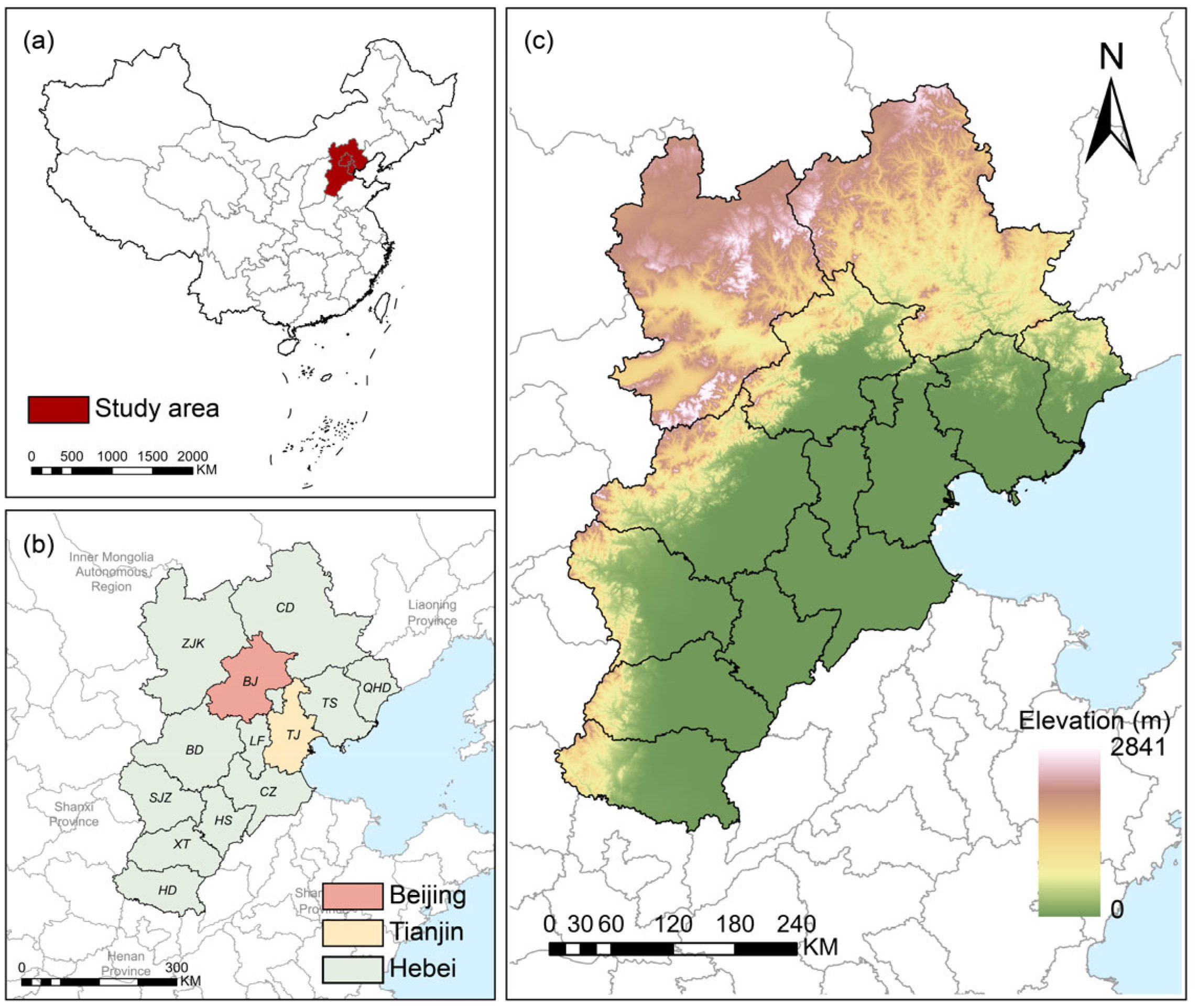
2.1. Study Area

The BTH urban agglomeration (113°04′–119°53′E, 36°01′–42°37′N) is located at the intersection of the North China Plain, the Taihang and Yan Mountains, and the Bohai Sea (Figure 1). It consists of Beijing, Tianjin, and Hebei Province, including Shijiazhuang, Baoding, Xingtai, Tangshan, Handan, Hengshui, Langfang, Cangzhou, Qinhuangdao, and Chengde. The terrain slope gradually slopes downward from northwest to southeast, with mountains dominating in the northwestern parts, while the southeast is primarily flat. The area has a temperate continental monsoon climate, with a marked seasonal precipitation pattern in precipitation that is mostly observed in the summer.

As reported by the Beijing Municipal Bureau of Statistics, the BTH region had a resident population of 1.1 × 10⁸ by the end of 2020, representing 7.8% of the total population in the country [58]. More specifically, the resident population of Beijing is 2.1 × 10⁷, that of Tianjin is 1.4 × 10⁷, and that of Hebei Province is 7.5 × 10⁷ million. The gross domestic product (GDP) of the BTH region totaled CNY 8.6 × 10¹² in 2020, marking an increase of 1.73% compared to the previous year [59].

2.2. Data Source

This study utilizes datasets encompassing land use/land cover, socio-economic, and climate data (

Table 1. Primary data list.

Data Name	Application	Spatial Resolution	Data Source
Land use type	FP, CS, WY, SC, HQ	30 m	China Land Cover Dataset [60]
Population	SED	1 km	Land Scan Global (https://landscan.ornl.gov/, accessed on 26 March 2025)
GDP	SED		Resource and Environment Science and Data Center (http://www.resdc.cn/, accessed on 26 March 2025)
Nightlight	SED		A Prolonged Artificial Nighttime Light Dataset of China (1984–2020) [61] 1 km monthly precipitation dataset for China (1901–2023) [62] 1 km monthly mean temperature dataset for China (1901–2023) [62] 1 km monthly potential evapotranspiration dataset for China (1901–2023) [63]
Precipitation	WY, SC, SED
Temperature	SED
Evapotranspiration	WY
Normalized Difference Vegetation Index (NDVI)	FP, SED	30 m	National Ecosystem Science Data Center (http://www.nesdc.org.cn/, accessed on 26 March 2025)
Digital elevation model (DEM)	SC	30 m	The Geospatial Data Cloud (https://www.gscloud.cn/, accessed on 26 March 2025)
Fractional Vegetation Cover (FVC)	SED	250 m	National Tibetan Plateau Data Center (https://data.tpdc.ac.cn/, accessed on 26 March 2025)
Root depth, soil texture, and organic carbon content	SC	1 km	China soil map-based harmonized world soil database (HWSD) (v1.1) (http://data.tpdc.ac.cn/zh-hans/data/611f7d50-b419-4d14-b4dd-4a944b141175/, accessed on 26 March 2025)
Food yield	FP	Province	China Statistical Yearbook (https://www.stats.gov.cn/sj/ndsj/2020/indexch.htm, accessed on 26 March 2025)

Note: FP indicates food production; CS indicates carbon storage; WY indicates water yield; SC indicates soil conservation; HQ indicates habitat quality; SED indicates social–environmental driver.

). All raster datasets were resampled to a 30 m × 30 m resolution and projected to the WGS 1984 UTM Zone 50 N using ArcGIS Pro (3.01).

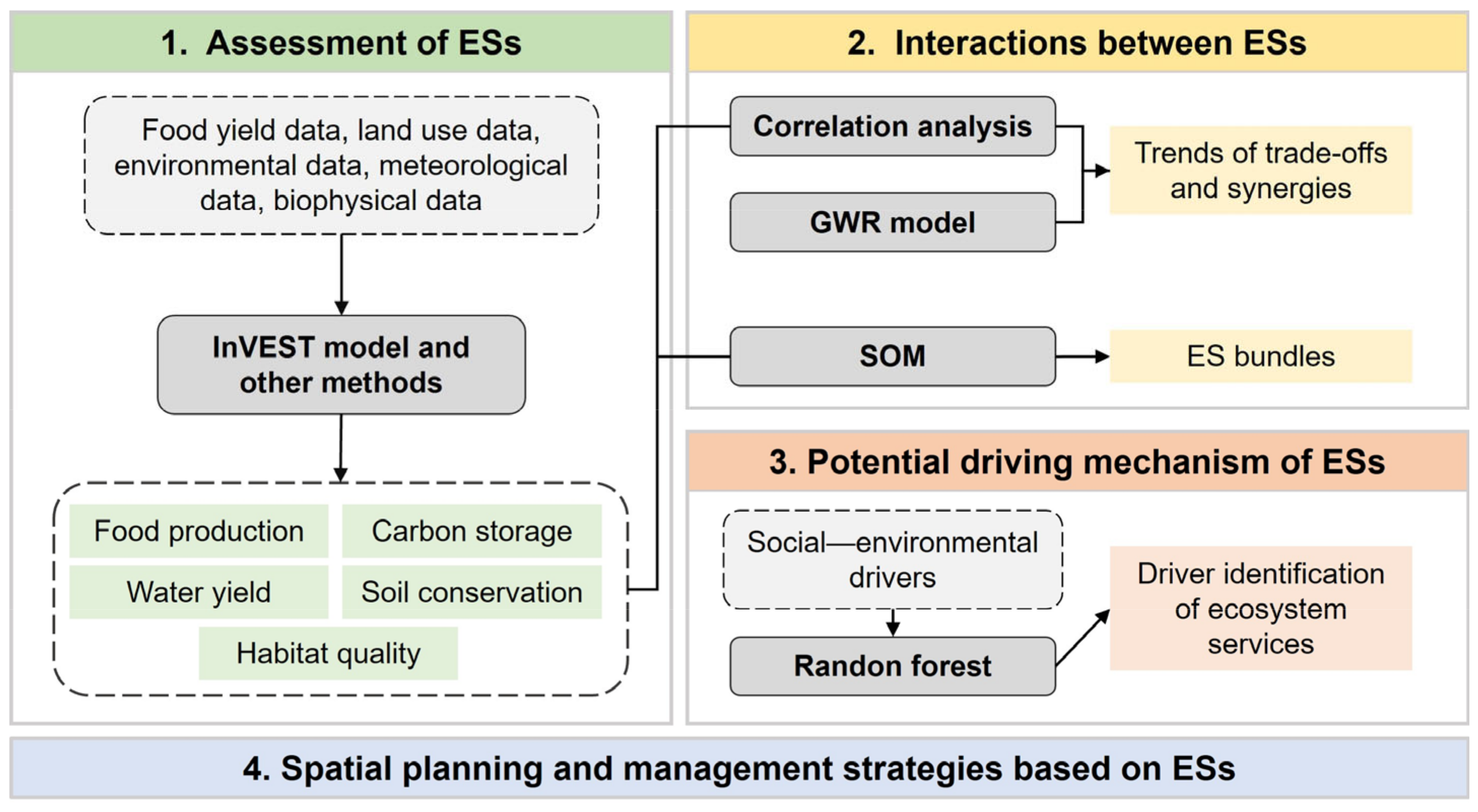
2.3. Research Framework

The research framework of this study comprises four components (Figure 2). First, the physical quantities of five ESs in the study area for 2000, 2010, and 2020 using the InVEST model are estimated, and the Ecosystem Services Index (ESI) is calculated through equal weighting and summation. Subsequently, based on the ES assessment results, we analyzed the spatiotemporal variations in trade-offs and synergies between ESs using correlation analyses and the GWR model. Additionally, SOM clustering was employed to identify ES bundles in the selected years by systematically examining their spatiotemporal distribution patterns and transitions. Finally, using these findings, this study proposes spatial planning and management recommendations for ES optimization in the BTH region.

2.4. Assessment of Ecosystem Services

We adhered to three key principles when selecting ESs for this study: (1) they had to be consistent with the classification of MEA [1]; (2) they were important in maintaining ecosystem stability in the BTH region; (3) their availability allowed for the quantification of the data. Based on these principles, we selected food product (FP), carbon storage (CS), water yield (WY), soil conservation (SC) and habitat quality (HQ) as ecosystem services. ESs were first quantified at the 30 m × 30 m raster scale for the years 2000, 2010, and 2020 and then averaged across ecosystem services at the 3 km × 3 km grid scale using the zonal statistics tool in the ArcGIS Pro 3.01 platform.

2.4.1. Food Production (FP)

Relevant studies have shown a significant relationship between food production and the NDVI [64]. After mapping the distribution of FP at the raster scale based on the NDVI and statistical data, we obtained the following equation:

$$\begin{array}{c}{\mathit{FP}}_{\mathit{i}}={\displaystyle \frac{{\mathit{NDVI}}_{\mathit{i}}}{\mathit{NDVI}\_\mathit{total}}}\times \mathit{F}\mathit{P}\end{array}$$

(1)

where ${\mathit{FP}}_{\mathit{i}}$ is the FP of grid i (t/km²); ${\mathit{NDVI}}_{\mathit{x}}$ is the NDVI of grid i; $\mathit{FP}$ is the grain production in the BTH region (t/hm²); and $\mathit{NDVI}\_\mathit{total}$ is the total NDVI in the BTH region.

2.4.2. Carbon Storage (CS)

In this study, the carbon storage and sequestration module of the InVEST model was used to quantify the carbon sequestration capacity of the study area. This module estimates regional carbon sequestration by considering the average carbon density across four carbon pool and land use types. Carbon density data (Table S1) were obtained from previous studies in similar study areas. The total carbon storage can be calculated as follows:

$$\begin{array}{c}{\mathit{C}\_\mathit{total}}_{\mathit{i}}={\mathit{C}\_\mathit{above}}_{\mathit{i}}+{\mathit{C}\_\mathit{below}}_{\mathit{i}}+{\mathit{C}\_\mathit{soil}}_{\mathit{i}}+{\mathit{C}\_\mathit{dead}}_{\mathit{i}}\end{array}$$

(2)

where ${\mathit{C}\_\mathit{total}}_{\mathit{i}}$ represents the total carbon storage at grid i (t/km²), ${\mathit{C}\_\mathit{above}}_{\mathit{i}}$ represents the above-ground carbon storage at grid i (t/km²), ${\mathit{C}\_\mathit{below}}_{\mathit{i}}$ represents the below-ground carbon storage at grid i (t/km²), ${\mathit{C}\_\mathit{soil}}_{\mathit{i}}$ represents the soil’s carbon storage at grid i (t/km²), and ${\mathit{C}\_\mathit{dead}}_{\mathit{i}}$ represents the dead organic matter carbon storage of grid i (t/km²).

2.4.3. Water Yield (WY)

The water supply service capacity of the study area was calculated using the Annual Water Yield module of the InVEST model. The parameters involved in this module can be found in Table S2, and water yield can be calculated using the following equation:

$$\begin{array}{c}{\mathit{Y}}_{\mathit{i}\mathit{j}}=\left(1-{\displaystyle \frac{{\mathit{A}\mathit{E}\mathit{T}}_{\mathit{i}\mathit{j}}}{{\mathit{P}}_{\mathit{i}}}}\right)\times {\mathit{P}}_{\mathit{i}}\end{array}$$

(3)

where ${\mathit{Y}}_{\mathit{i}\mathit{j}}$ is the water yield of land use type j at pixel i (mm), ${\mathit{A}\mathit{E}\mathit{T}}_{\mathit{i}\mathit{j}}$ is the actual evapotranspiration of land use type j at pixel i (mm), and ${\mathit{P}}_{\mathit{i}}$ is the precipitation at pixel i.

2.4.4. Soil Conservation (SC)

We used the revised universal soil loss equation (RUSLE), which is based on the difference between potential and actual soil erosion values. The model parameters are provided in Table S3, and soil conservation can be calculated using the following equation:

$$\begin{array}{c}{\mathit{SC}}_{\mathit{i}}={\mathit{RKLS}}_{\mathit{i}}-{\mathit{USLE}}_{\mathit{i}}={\mathit{R}}_{\mathit{i}}\times {\mathit{K}}_{\mathit{i}}\times \left(1-\mathit{LS}\times {\mathit{C}}_{\mathit{j}}\times {\mathit{P}}_{\mathit{j}}\right)\end{array}$$

(4)

where ${\mathit{SC}}_{\mathit{i}}$ represents annual soil conservation at grid i (t/km²); ${\mathit{RKLS}}_{\mathit{i}}$ and ${\mathit{USLE}}_{\mathit{i}}$ represent the potential and actual soil erosion at grid I (t/km²), respectively; ${\mathit{R}}_{\mathit{i}}$ represents rainfall erosivity at grid i (MJ⋅mm/km²⋅h), ${\mathit{K}}_{\mathit{i}}$ represents soil erodibility at grid i (t⋅km²⋅h/ km²⋅MJ⋅mm); $\mathit{L}\mathit{S}$ represents the slope length gradient factor for land use type j (dimensionless); ${\mathit{C}}_{\mathit{j}}$ represents the vegetation coverage factor (dimensionless); and ${\mathit{P}}_{\mathit{j}}$ represents the support practice factor for land use type j (dimensionless).

2.4.5. Habitat Quality (HQ)

We selected the habitat quality index to assess habitat quality using the InVEST model, which is commonly employed to assess habitat maintenance capacity due to its user-friendliness and high availability parameters. The parameters are shown in Tables S4 and S5, and habitat quality can be calculated using the following equation:

$$\begin{array}{c}{\mathit{Q}}_{\mathit{ij}}={\mathit{H}}_{\mathit{j}}\times \left[1-{\displaystyle \frac{{\mathit{D}}_{\mathit{ij}}^{\mathit{z}}}{\left({\mathit{k}}^{\mathit{z}}+{\mathit{D}}_{\mathit{ij}}^{\mathit{z}}\right)}}\right]\end{array}$$

(5)

where ${\mathit{Q}}_{\mathit{ij}}$ represents habitat quality (dimensionless), ${\mathit{H}}_{\mathit{j}}$ represents habitat suitability (dimensionless), ${\mathit{D}}_{\mathit{ij}}$ represents the threat level (dimensionless), z and k represent scaling parameters (or constants), i represents the grid, and j represents the land use type.

2.4.6. Ecosystem Service Index

In this study, the ESI was used to quantify the comprehensive provisioning capacity of multiple ESs. The overall ES was obtained by normalizing the five aforementioned ESs with equal weighting. The equation to calculate the ESI is as follows:

$$\begin{array}{c}{\mathit{ESI}}_{\mathit{i}}={\displaystyle \sum _{\mathit{n}=1}^5}{\mathit{ES}}_{\mathit{in}}\times {\mathit{w}}_{\mathit{n}}\end{array}$$

(6)

where ${\mathit{ESI}}_{\mathit{i}}$ is the integrated supply of ecosystem services at raster i, ${\mathit{ES}}_{\mathit{in}}$ is the n-th ES at raster i, and ${\mathit{w}}_{\mathit{n}}$ is the weight of the n-th ES.

2.5. Identification of Trade-Offs/Synergies Between ESs

2.5.1. Correlation Analysis

After quantifying all five ESs, the results of pixel-level calculations for several services were integrated to a grid scale (3 km × 3 km). Spearman correlation analyses were performed to assess the relationships between ESs, where negative correlation coefficients indicated trade-offs between the two services, while positive coefficients suggested synergies. The analyses were carried out using the “Hmisc” package in R (version 4.4.0) [20,25].

2.5.2. Geographically Weighted Regression

In addition to evaluating ecosystem service relationships through correlation analyses, we investigated their spatial patterns using GWR. The GWR coefficients revealed interactions between ESs, where negative values indicated spatial trade-offs, while positive values represented spatial synergies. The GWR model is a local linear regression technique used to identify spatial variable relations; it is based on the assumption that significant spatial heterogeneities or non-stationary features exist in spatial data relationships [65]. The “GWmodel” package for R (version 4.4.0) was used to analyze the GWR model. The equation of the GWR model is as follows:

$$\begin{array}{c}{\mathit{y}}_{\mathit{i}}={\mathsf{\beta }}_0\left({\mathsf{\mu }}_{\mathit{i}},{\mathit{v}}_{\mathit{i}}\right)+{\displaystyle \sum _{\mathit{k}=1}^{\mathit{p}}}{\mathsf{\beta }}_{\mathit{k}}\left({\mathsf{\mu }}_{\mathit{i}},{\mathit{v}}_{\mathit{i}}\right){\mathit{x}}_{\mathit{ik}}+{\mathsf{\epsilon }}_{\mathit{i}}\end{array}$$

(7)

where ${\mathit{y}}_{\mathit{i}}$ is the dependent variable at grid i; $\left({\mathsf{\mu }}_{\mathit{i}},{\mathit{v}}_{\mathit{i}}\right)$ is the spatial position at grid i; ${\mathsf{\beta }}_0\left({\mathsf{\mu }}_{\mathit{i}},{\mathit{v}}_{\mathit{i}}\right)$ is the intercept at grid i; ${\mathsf{\beta }}_{\mathit{k}}\left({\mathsf{\mu }}_{\mathit{i}},{\mathit{v}}_{\mathit{i}}\right)$ is the regression coefficient; ${\mathit{x}}_{\mathit{ik}}$ is the dependent variable at grid i; p is the number of independent variables; and ${\mathsf{\epsilon }}_{\mathit{i}}$ denotes random errors at grid i.

2.6. Identification of ES Drivers

Based on a synthesis of previous research, we selected 10 representative socio-ecological drivers which were subsequently categorized into three distinct groups according to their inherent characteristics: natural, social, and land use factors (

Table 2. Social–environmental drivers.

Category	Driving Factor	Unit
Natural factors	Precipitation (X1)	mm
	Temperature (X2)	°C
	FVC (X3)	%
Social factors	Nightlight (X4)	Dimensionless
	Population density (X5)	People/km2
	GDP (X6)	Ten thousand yuan/km2
Land use factors	Cropland area ratio (X7)	%
	Forest area ratio (X8)	%
	Grassland area ratio (X9)	%
	Impervious area ratio (X10)	%

).

The RF model is a supervised machine learning algorithm with robust generalization and consistent performance. Its effectiveness in addressing multicollinearity issues and evaluating the importance of independent variables has contributed to its widespread application in ecological research. [28,29,66]. In this study, the RF model is applied to select the driver’s contribution to ESs. We used “randomForest” package in R (version 4.4.0) to analyze the RF model.

2.7. Identification of ES Bundles

An SOM is an unsupervised artificial neural network developed by Kohonen in 1984. It maps high-dimensional data to low-dimensional space and enables data clustering and visualization. We applied SOMs to identify ESs with similar spatial distributions and divide ES bundles based on similarity. To maintain the comparability and coherence of ES bundles, we standardized the ES values for the three years during which the SOM was implemented in order to identify ES bundles. We used the “Kohonen” package in R (version 4.4.0) to analyze SOMs.

3. Results

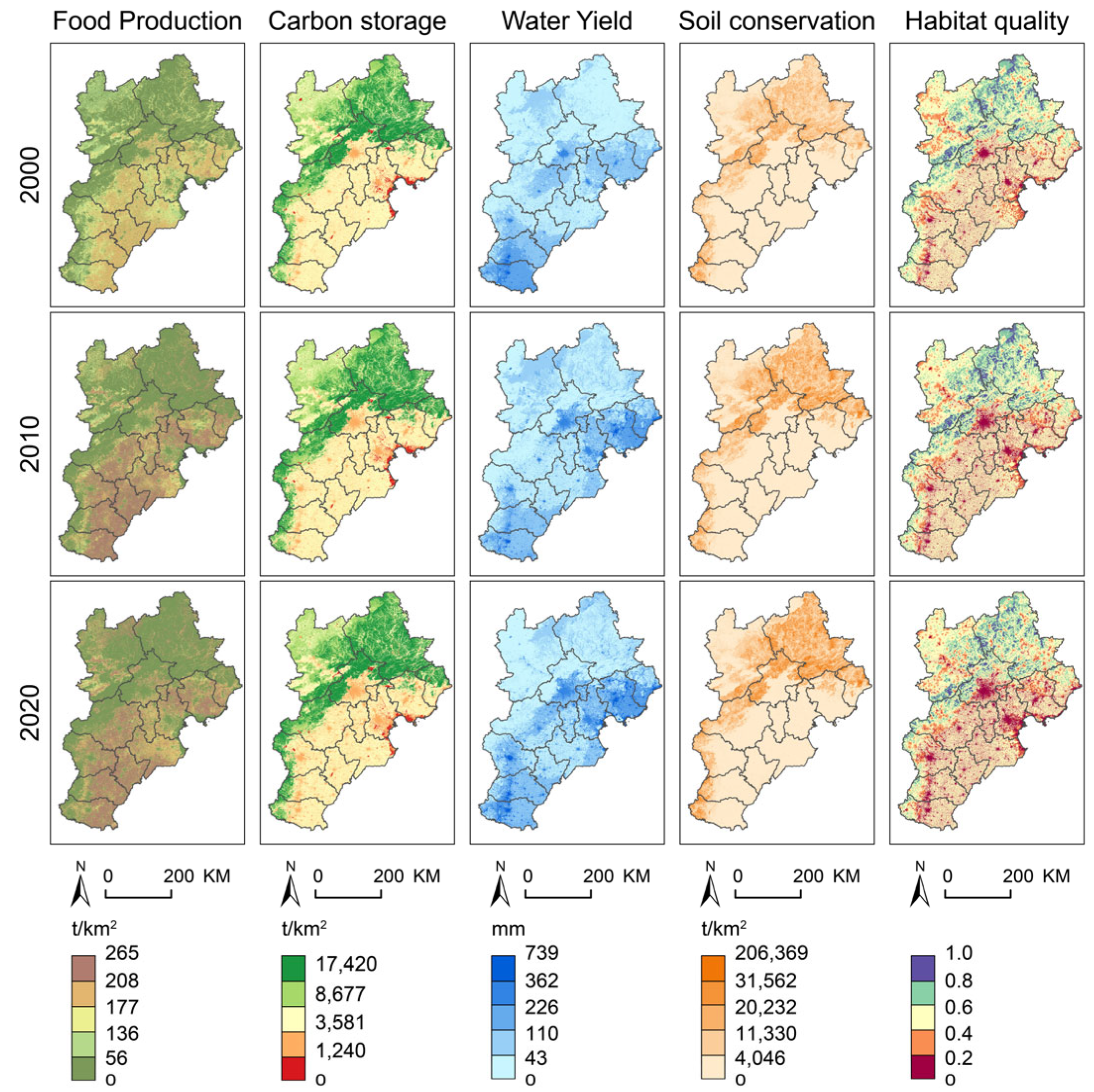
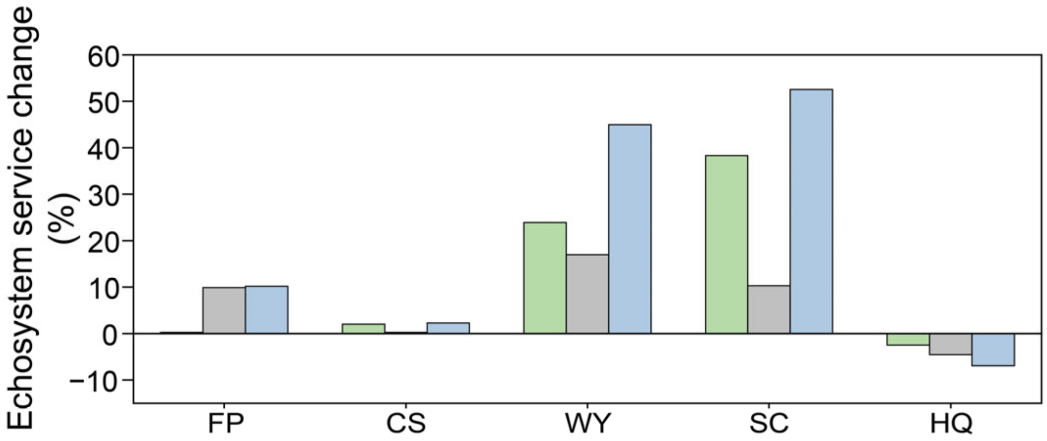
3.1. Spatial and Temporal Distribution Patterns of ESs

As seen in Figure 3, the five ESs in the BTH region remain relatively constant over time, but they exhibit notable spatial heterogeneity in their distributions. CS, SC, and HQ show similar spatial distributions in space, with no significant annual variations observed. Specifically, the northwestern mountainous areas had high values of ES supply. The high-supply area of FP is centralized along the southeastern plains, which was the primary grain-producing area of the BTH region. Throughout the study period, the total grain production in the BTH region exhibited an upward trend, with a distinct increase in grain yield per unit area in the plains. From 2000 to 2020, the spatial distribution of WY in the BTH region was characterized by high levels in the central and southern plains and eastern coastal areas, and low levels in the northwestern mountainous areas, with significant annual variations in the distributions.

Overall, all four ESs increased from 2000 to 2020 (Figure 4), except for HQ, which decreased. The mean values of WY and SC increased by 23.93% and 38.32%, respectively, from 2000 to 2010, and by 16.99% and 10.30%, respectively, from 2010 to 2020. No significant changes were found for the mean value of FP between 2000 and 2010. However, a notable increase in the growth rate occurred during the subsequent period from 2010 to 2020, reaching 10.18%. Similarly, the mean value of CS remained relatively constant throughout the entire observation period. In contrast, the mean value of HQ continued to decrease from 2000 to 2020, exhibiting a progressively accelerating decline.

3.2. Land Use Change Patterns

The land use cover and its changes in the BTH region are presented in Figure 5. The proportions of each land use type in the study area, listed in descending order, are cropland, forest, grassland, impervious land, water, and bare land. During the study period, both forest and impervious land exhibited an expansion trend, whereas the other land use types showed a decreasing share. Specifically, construction land expanded by 1.08 × 10⁴ km², reflecting a 49.58% increase, while cropland decreased by 1.17 × 10⁴ km², with an 11.04% decline. Regarding land use conversions, the reduction in cropland was predominantly due to its conversion into impervious land, with an area of 9506.97 km², accounting for 57.98% of the total decrease in cropland area. The total area of grassland converted to other land types was 9779.38 km², representing 26.76% of the grassland area in 2000, with 62.61% of this area being transferred to forest. Between 2000 and 2020, the area of impervious land increased by 49.58%, with the expansion of impervious land most notably observed in Beijing, Tianjin, and Shijiazhuang, regions experiencing rapid urbanization.

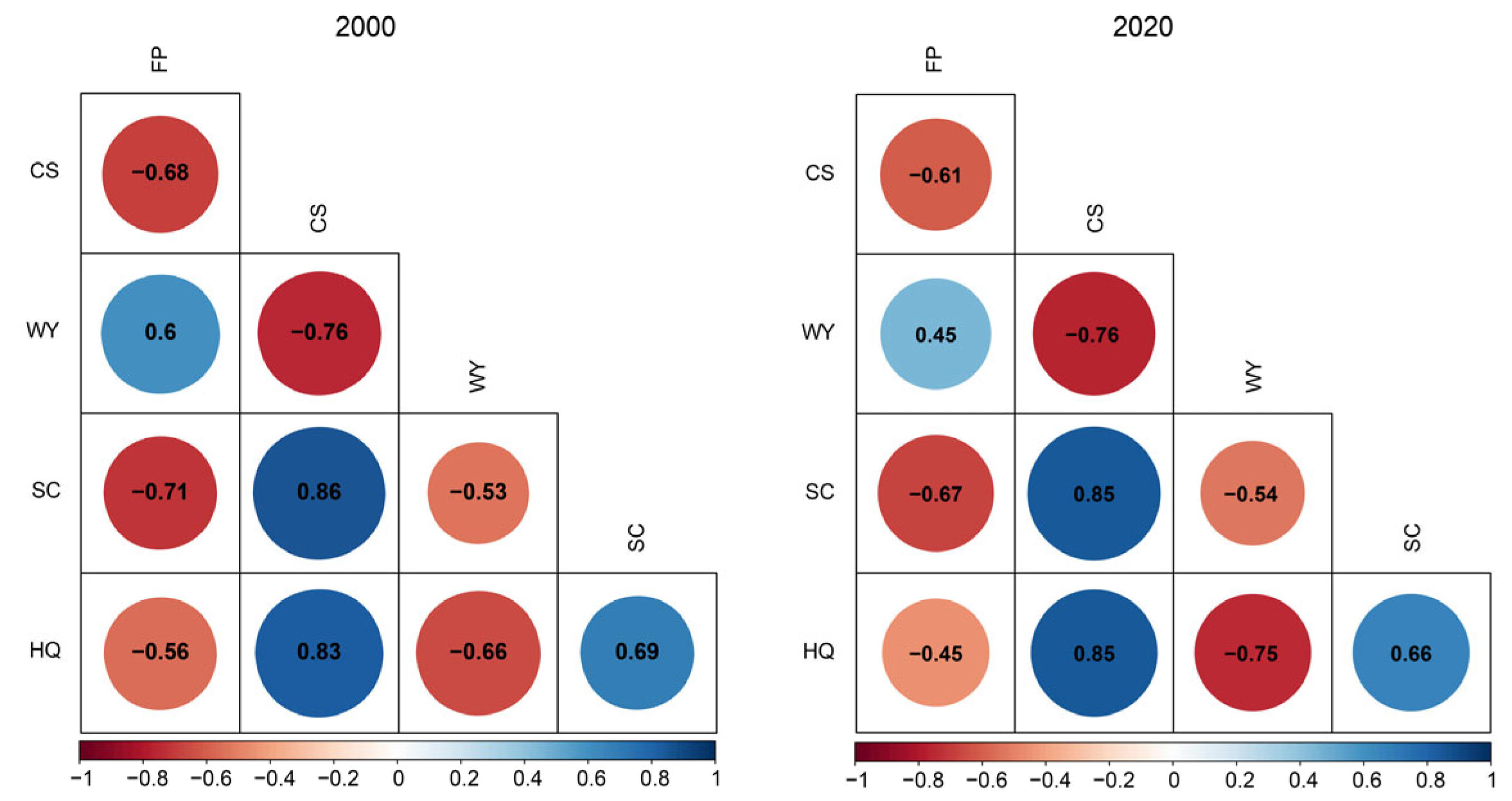
3.3. Trade-Offs and Synergies Among ESs

There were 10 significant correlations found among the five ESs, with all correlations showing statistical significance (p < 0.05). Among these, six pairs had negative correlations and four pairs had positive correlations. The correlations observed between ES pairs were similar across the two years (Figure 6). Between 2000 and 2020, the level of synergy among the majority of ESs grew, whereas the extent of trade-offs diminished.

The GWR model results showed that the spatial patterns of trade-offs and synergies in ES pairs exhibited significant heterogeneity (Figure 7). The relationships of FP-WY, SC-HQ, CS-SC, and CS-HQ were dominated by spatial synergies, with FP-WY, CS-SC, and SC-HQ primarily observed in the northwestern mountainous areas.

On the other hand, the ES pairs of FP-CS, WY-SC, FP-SC, CS-WY, FP-HQ, and WY-HQ were primarily characterized by trade-offs rather than synergies; in particular, the WY-HQ trade-off was notably pronounced. In 2000, significant spatial trade-offs for WY-HQ were distributed over the entire study area. By 2020, the extent of high trade-offs in the WY-HQ region had decreased, with the remaining areas being more sporadically distributed in the eastern and southern areas.

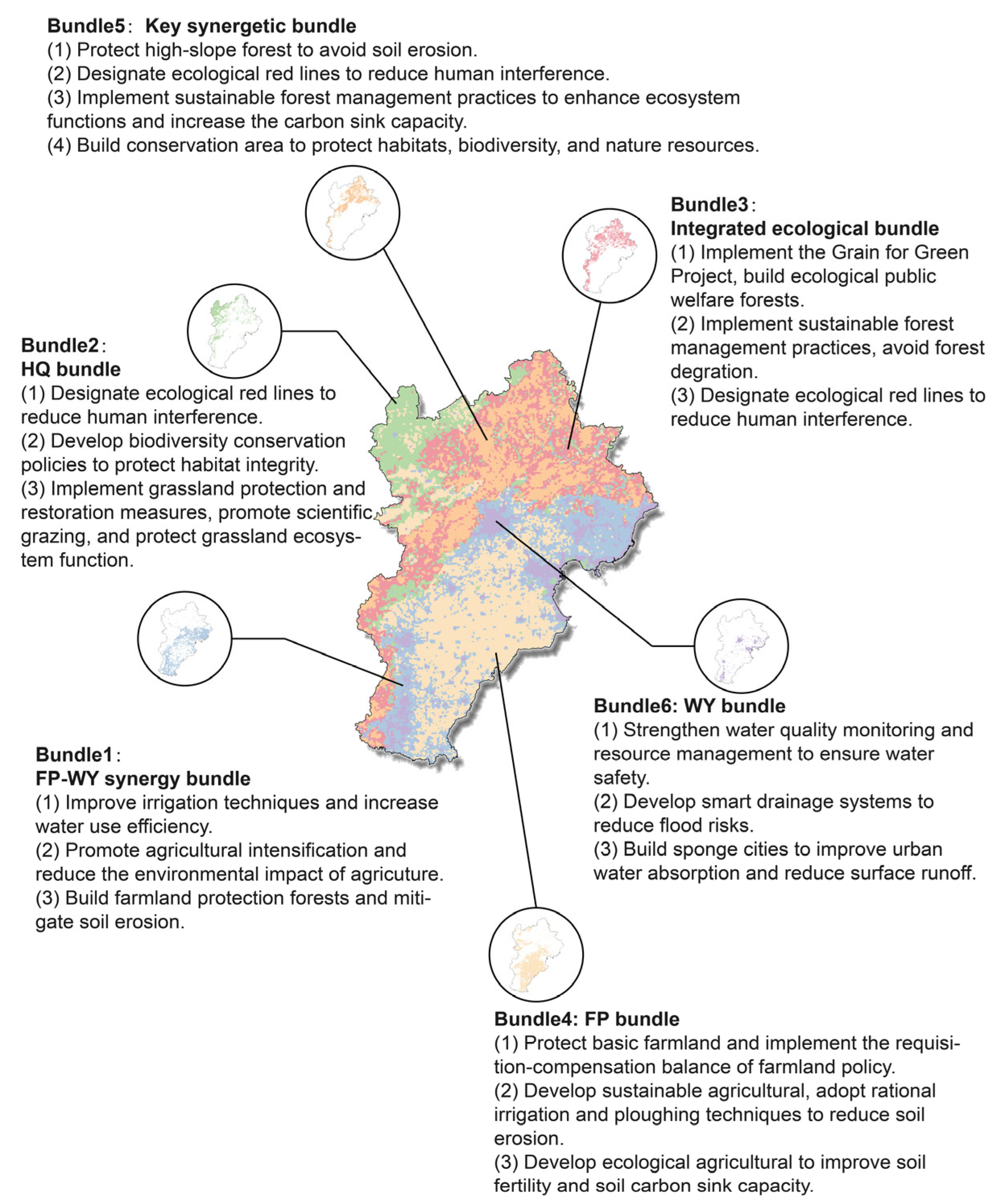
3.4. ES Bundle Characteristics and Distribution

Six ES bundles in BTH were identified via SOMs in 2000, 2010, and 2020 (Figure 8). The spatial–temporal distribution characteristics of the six ES bundles are as follows: Bundle 1, with a total value of 1.9, shifted its distribution from predominantly southern to eastern coastal areas. The scores for FP (0.52) and WY (0.63) were the highest in Bundle 1, together accounting for over 60% of the total value. Bundle 2, with a total value of 1.76, displayed a relatively even distribution across the six ESs and was primarily found in the Bashang Plateau, showing minimal spatial and temporal variation. Bundle 3 had a total value of 2.19 and was mostly concentrated along the Taihang Mountain, with the highest scores observed in CS (0.61), SC (0.54), and HQ (0.51), representing 75.8% of the total value. Bundle 4 was mainly distributed in the North China Plain, where FP (0.62) had the highest score, and this bundle also exhibited the highest proportion among the six bundles. Bundle 5 had the highest total value (2.68) among the six bundles and was mainly distributed in the northwest mountainous region, where CS, SC, and HQ were the most prominent services. Bundle 6 was mainly distributed in areas with impervious land and the eastern coastal region. Its WY was the highest of the six bundles. In general, Bundle 1 and 4 were characterized by a predominance of regulating services, while Bundle 2 had the lowest total ESs. Bundle 3 and 5 predominantly included regulating and supporting services, whereas Bundle 6 was dominated by supplying services.

3.5. Impacts of Driving Factors on ESs

We analyzed the impact of socio-ecological factors on the functioning of ecosystem services based on the feature importance ranking in the RF model (Figure 9). The results revealed the following:

(a)

FP was mainly driven by precipitation, FVC, and the cropland area ratio. The effects of all three drivers weakened across time, but the effects of nightlight, population density, and the forest area ratio increased.

(b)

CS was mainly driven by forest area, grassland area, and cropland area ratios. The degree of the influence of grassland increased over time, while the effect of the cropland area ratio was inversely related to time.

(c)

In 2000, the dominant drivers for WY were precipitation and cropland area and forest area ratios, while in 2020, the dominant drivers were precipitation and impervious area and forest area ratios. Over the 20-year period, the InMSE for the impervious area ratio increased by 54.80%.

(d)

SC was driven by precipitation, DGP, and the forest area ratio in 2000, which was the same in 2020. In particular, the influence of precipitation decreased over time, while the impact of the other two factors increased.

(e)

The impact of all ten drivers on HQ was more pronounced, but the primary drivers were the impervious area ratio, FVC, and precipitation. Additionally, the influence of landscape factors (particularly the impervious area ratio) on HQ increased significantly.

(f)

ESs were primarily driven by precipitation, FVC, and the cropland area ratio. From 2000 to 2020, the contribution of precipitation, population density, and grassland area and impervious area ratios showed an increasing trend, with the precipitation InMSE increasing by 78.72%.

4. Discussion

4.1. The Characteristics and Distributions of ES Interactions

In this study, trade-offs, synergies, and ES bundles were used as indicators to investigate the interactions between ESs. Determining the spatial–temporal variations and the interactions among ESs is crucial for effective ecosystem management [35]. The spatial patterns of ESs in this study were consistent with those observed in prior research [6,8,56]. In terms of spatial distribution, CS, SC, and HQ exhibited comparable patterns. The high supply of ES areas was primarily situated in the northern and western mountainous regions. The high altitude and low human activity in these regions provide favorable ecological conditions. In addition, the northern mountainous region falls within the scope of the Three-North Shelterbelt Forest Program. Since 2000, various ecological conservation and restoration initiatives, including afforestation, have been implemented in this region, leading to significant increases in ecosystem services [67,68]. In contrast, the central and southeastern plains, which are predominantly cropland areas, showed higher FP values. The urban built-up areas, on the other hand, exhibited higher WY values due to low permeability and limited evaporation in the absence of vegetation [8]. The trade-off and synergy among these ESs align with earlier studies [6]. The results indicate a declining trend in the synergies of ES pairs, which should be taken into account in ES management strategies.

The ES bundle with the highest value was predominantly found in the northwestern mountainous region. This area, characterized by high vegetation cover, favorable natural resource conditions, and minimal human activity, supports robust ecosystem service functions. However, Bundle 2 and 5, which had the lowest values, were primarily distributed in the alpine meadow regions of the northwest plateau and urban built-up areas. Bundle 6 showed significantly lower values compared to the average for all ESs except for WY. The spatial distribution of Bundle 6 largely overlapped with the areas designated as impervious, revealing the poorly integrated ESs in urban built-up areas. This emphasizes that more attention should be paid to effective ecosystem management within the context of urban development. Bundle 4 was primarily characterized by FP, and its distribution showed a strong correlation with croplands, making it the most dominant ES bundle in the BTH region. Previous studies regarding ES bundles have also delineated separate FP bundles [25,42,46,69]. Since Bundle 4 is the most dominant ES bundle in the BTH region and FP involves trade-offs with most other ESs, which are findings consistent with previous studies, these trade-offs should be considered in ES management [36,70,71].

ES bundles can reflect ecosystem states, and understanding shifts in these bundles can provide valuable insights into ecosystem changes [72]. We analyzed the spatial and temporal changes in ES bundles (Figure 6) and found that Bundle 1 exhibited spatial and temporal heterogeneity, with its proportion continuously increasing over 20 years, while its spatial distribution shifted from a concentration in the south to a more widespread distribution along the eastern coast. By comparing the changes in land use and ES bundles across the BTH region, we observed that Bundle 1 was predominantly concentrated around urban built-up areas. The interrelationship of ES bundle transformations indicated that the transformation pattern among Bundles 1, 4, and 6 follows a progression from Bundle 4 to Bundle 1 and from Bundle 1 to Bundle 6, which aligns with the trend of urban expansion from the center outward. This pattern reflects the close relationship between urban expansion and the transformation of ES bundles [73]. Within the context of urbanization, exploring the drivers of ES bundle transitions is essential to comprehensively understand changes in ecosystem structures. Consequently, future studies should focus on exploring the mechanisms behind the spatial and temporal variations in these ES bundles.

4.2. Potential Driving Mechanisms of ESs

Social–environmental factors significantly influence the variation in ESs [74]. Understanding how these factors affect ecosystem services can guide urban planning and development approaches, leading to more efficient ecosystem management [18,69].

CS was primarily affected by land use types, with forest, grassland, and cropland playing crucial roles in enhancing carbon sequestration. Additionally, social factors exhibited a negative correlation with CS, indicating that population growth, economic development, and urban expansion contributed to the degradation in CS supply [9]. Therefore, urban planning should prioritize the expansion of ecological land, such as artificial wetlands and urban green spaces, to enhance the carbon sequestration potential of urban ecosystems. WY was positively correlated with precipitation, i.e., an increase in precipitation corresponded to an increase in water yield. This is attributed to the monsoonal climate in the BTH region, where precipitation exhibited uneven spatial and temporal distribution along with significant interannual variability. As a result, the WY in 2020 was higher compared to 2000 and 2010. Under similar climatic conditions, the WY on vegetated surfaces was lower than that on impervious surfaces [75]. Therefore, the WY in urban built-up areas was greater than in forests, leading to spatial differences in WY distribution across the BTH region.

The proportional allocation of land use plays a significant role in balancing ecosystem services [76]. In the BTH region, a noticeable pattern emerged, with an increase in both impervious and forest lands, while cropland, grassland, and water areas diminished. An examination of the driving factors of land use indicated a positive relationship between the forest area ratio and the ESI, whereas the impervious area and grassland area ratios exhibited negative correlations with the ESI. After the implementation of the Three-North Shelter Forest Program and the farmland requisition compensation balance policy, forest land growth positively enhanced the regional ecosystem service supply. However, rapid urban expansion led to a decline in ESs. Therefore, addressing the conflict between socio-economic development and ecosystem functions, as well as promoting their coordinated development, is crucial for achieving sustainable development.

4.3. Spatial Planning and Management Strategies

This study presents an in-depth examination of the features and spatial–temporal changes in ES bundles. Based on the distribution patterns observed in 2020, we suggest spatial planning and management approaches for the BTH region (Figure 10).

Notably, Bundle 1 exhibited a synergistic relationship for WY-FP, but the spatial–temporal analysis reflected a declining trend in their relationship (Figure 6 and Figure 7). As a result, we recommend targeted actions within this bundle to improve soil and water conservation capabilities, highlighting the importance of incorporating spatial–temporal analyses of ES interactions into urban spatial planning [25]. However, Bundle 2 showed the lowest ES supply, and regarding its spatial distribution of land use, we found that Bundle 2 was primarily distributed in grassland. Therefore, we propose the implementation of protection and restoration policies to strengthen the function of grassland ecosystems. Bundles 3 and 5 are highly synergistic, and effective management of individual or multiple ecosystem service functions can significantly enhance the performance of other services [42]. Bundle 3 exhibited CS-SC-HQ synergies, and it is primarily distributed in the transition zone from high-altitude forests to other land types, especially cropland; consequently, we propose the implementation of policies to restore farmland to forests and designate ecological red lines to ensure the ecosystem stability of the area with a high ES supply. Bundle 5 exhibited the highest ES supply capacity, which was primarily characterized by the synergies among CS, SC, and HQ. The proportion of Bundle 5 increased significantly between 2000 and 2010, remaining relatively stable from 2010 to 2020. Therefore, ES management should focus on preserving the stability of Bundle 5. Bundle 3 gradually transitioned to Bundle 5 over the study period, reflecting the positive outcomes of ecological protection initiatives, such as the Three-North Shelterbelt Program and Grain for Green Project, in mountainous areas.

Bundle 4 was characterized by FP, indicating that the supply of other ESs was low in regions with high FP; this suggests a trade-off between FP and other ESs, which is a finding supported by previous studies [77,78,79]. The distribution of Bundle 4 closely aligns with cropland that is primarily located in the eastern and southern plains. These areas are characterized by flat terrain at low elevations and a high concentration of towns, villages, and farmland. The predominant land use types in these regions are arable and construction land, which serve as the primary food supply zones within the BTH region. Bundle 6 demonstrated a high supply of WY and a low supply of other ESs. In the trade-off/synergy analysis of WY and other services, WY and all other ESs, except FP, exhibited a trade-off relationship, which intensified over time. Furthermore, the spatial distribution of Bundle 6 was highly consistent with the distribution of impervious land. If urban expansion continues, the proportion of Bundle 6 in the study area may increase, potentially leading to a decline in the overall ecosystem service function. Consequently, Bundle 6 should be prioritized in future ecological spatial management strategies.

Undoubtedly, grid-based planning and management approaches provide greater detail, and the previous study presented strategies for managing county-level ES bundles in the BTH region [42]. Shen compared multi-scale ES bundles in the BTH region but did not account for temporal changes [24]. In contrast, this study proposes urban spatial management and planning at the grid scale for the BTH region, informed by the variations in ESs and ES bundles from 2000 to 2020. The proposed strategies emphasize spatial intricacies in the BTH region.

4.4. Limitations

This study lacks research into the impact of various drivers on ESs at multiple spatial scales, focusing only on the supply of ESs. Future research could explore the balance between the supply and demand of ESs at multiple spatial levels. Additionally, the findings of this study indicate a close relationship between ESs and land use change, suggesting that future multi-scenario studies could simulate the supply–demand dynamics of ESs based on land use change across different scales. Furthermore, although the InVEST model is widely used in ES assessment because of its suitability, it has certain limitations [80]. Future studies should incorporate other land surface models, such as the CASA model and soil and water conservation models, to examine ecological processes.

5. Conclusions

This study proposes a grid-scale analytical framework integrating the InVEST-GWR-RF-SOM to systematically assess spatial–temporal dynamics of ES trade-offs/synergies and ES bundles while also exploring the socio-ecological factors influencing changes in ES. Specifically, the overall ecosystem services in the BTH region demonstrated an increasing trend, with the exception of HQ, which exhibited a declining trend. Spatial heterogeneity in ES provision was evident, with high-supply areas primarily located along mountain ranges, and low-supply areas in the plains, which expanded as urban built-up areas grew. This suggests that greater attention should be paid to the degradation of ES functions resulting from urban expansion. Furthermore, trade-off relationships among ESs dominated during the study period, with FP and WY showing strong trade-offs with other services. Additionally, ESs were influenced by socio-ecological factors, with precipitation, FVC, and land use being the most significant factors affecting the ESI. Over time, the impact of natural and landscape factors on ESs strengthened, while the influence of social factors diminished. We proposed urban spatial management and planning suggestions based on the change trends of ES interactions and socio-ecological drivers to inform the sustainable development of regional ecosystems.

References

1. Millennium Ecosystem Assessment (MEA). Ecosystems and Human Wellbeing: Synthesis; Island Press: Washington, DC, USA, 2005. [Google Scholar]
2. Costanza, R.; Grasso, M.; Hannon, B.; Limburg, K.; Naeem, S.; O’Neill, R.V.; Paruelo, J.; Raskin, R.G.; Sutton, P. The Value of the World’s Ecosystem Services and Natural Capital. Ecol. Econ. 1998, 25, 3–15. [Google Scholar]
3. Liu, Y.; Xia, C.; Ou, X.; Lv, Y.; Ai, X.; Pan, R.; Zhang, Y.; Shi, M.; Zheng, X. Quantitative Structure and Spatial Pattern Optimization of Urban Green Space from the Perspective of Carbon Balance: A Case Study in Beijing, China. Ecol. Indic. 2023, 148, 110034. [Google Scholar] [CrossRef]
4. Yang, J.; Duan, C.; Wang, H.; Chen, B. Spatial Supply-Demand Balance of Green Space in the Context of Urban Waterlogging Hazards and Population Agglomeration. Resour. Conserv. Recycl. 2023, 188, 106662. [Google Scholar] [CrossRef]
5. Vihervaara, P.; Rönkä, M.; Walls, M. Trends in Ecosystem Service Research: Early Steps and Current Drivers. AMBIO 2010, 39, 314–324. [Google Scholar] [CrossRef]
6. Ai, X.; Zheng, X.; Zhang, Y.; Liu, Y.; Ou, X.; Xia, C.; Liu, L. Climate and Land Use Changes Impact the Trajectories of Ecosystem Service Bundles in an Urban Agglomeration: Intricate Interaction Trends and Driver Identification under SSP-RCP Scenarios. Sci. Total Environ. 2024, 944, 173828. [Google Scholar] [CrossRef]
7. Ouyang, X.; Tang, L.; Wei, X.; Li, Y. Spatial Interaction between Urbanization and Ecosystem Services in Chinese Urban Agglomerations. Land Use Policy 2021, 109, 105587. [Google Scholar] [CrossRef]
8. Li, T.; Jia, B.; Zhang, Q.; Liu, W.; Fang, Y. Scenario Simulation of Urban Land Use and Ecosystem Service Coupling Major Function-Oriented Zoning. Ecosyst. Health Sustain. 2024, 10, 0078. [Google Scholar] [CrossRef]
9. Li, S.; Yang, H.; Liu, J.; Lei, G. Towards Ecological-Economic Integrity in the Jing-Jin-Ji Regional Development in China. Water 2018, 10, 1653. [Google Scholar] [CrossRef]
10. Behboudian, M.; Anamaghi, S.; Mahjouri, N.; Kerachian, R. Enhancing the Resilience of Ecosystem Services under Extreme Events in Socio-Hydrological Systems: A Spatio-Temporal Analysis. J. Clean. Prod. 2023, 397, 136437. [Google Scholar] [CrossRef]
11. Yang, Q.; Liu, G.; Casazza, M.; Dumontet, S.; Yang, Z. Ecosystem Restoration Programs Challenges under Climate and Land Use Change. Sci. Total Environ. 2022, 807, 150527. [Google Scholar] [CrossRef]
12. Ouyang, Z.; Wang, X.; Miao, H. A Primary Study on Chinese Terrestrial Ecosystem Services and Their Ecological-Economic Values. Acta Ecol. Sin. 1999, 19, 607–613. [Google Scholar]
13. Jiang, W.; Wu, T.; Fu, B. The Value of Ecosystem Services in China: A Systematic Review for Twenty Years. Ecosyst. Serv. 2021, 52, 101365. [Google Scholar] [CrossRef]
14. Xie, G.; Zhang, C.; Zhen, L.; Zhang, L. Dynamic Changes in the Value of China’s Ecosystem Services. Ecosyst. Serv. 2017, 26, 146–154. [Google Scholar] [CrossRef]
15. Yang, M.; Chen, Y.; Yang, Y.; Yan, Y. Nonlinear Relationship and Threshold-Based Zones between Ecosystem Service Supply-Demand Ratio and Land Use Intensity: A Case Study of the Beijing-Tianjin-Hebei Region, China. J. Clean. Prod. 2024, 481, 144148. [Google Scholar] [CrossRef]
16. Braun, D.; de Jong, R.; Schaepman, M.E.; Furrer, R.; Hein, L.; Kienast, F.; Damm, A. Ecosystem Service Change Caused by Climatological and Non-Climatological Drivers: A Swiss Case Study. Ecol. Appl. 2019, 29, e01901. [Google Scholar] [CrossRef]
17. Reader, M.O.; Eppinga, M.B.; de Boer, H.J.; Damm, A.; Petchey, O.L.; Santos, M.J. Biodiversity Mediates Relationships between Anthropogenic Drivers and Ecosystem Services across Global Mountain, Island and Delta Systems. Glob. Environ. Change 2023, 78, 102612. [Google Scholar] [CrossRef]
18. Shen, J.; Li, S.; Wang, H.; Wu, S.; Liang, Z.; Zhang, Y.; Wei, F.; Li, S.; Ma, L.; Wang, Y.; et al. Understanding the Spatial Relationships and Drivers of Ecosystem Service Supply-Demand Mismatches towards Spatially-Targeted Management of Social-Ecological System. J. Clean. Prod. 2023, 406, 136882. [Google Scholar] [CrossRef]
19. Dade, M.C.; Mitchell, M.G.E.; McAlpine, C.A.; Rhodes, J.R. Assessing Ecosystem Service Trade-Offs and Synergies: The Need for a More Mechanistic Approach. Ambio 2019, 48, 1116–1128. [Google Scholar] [CrossRef]
20. Dou, H.; Li, X.; Li, S.; Dang, D.; Li, X.; Lyu, X.; Li, M.; Liu, S. Mapping Ecosystem Services Bundles for Analyzing Spatial Trade-Offs in Inner Mongolia, China. J. Clean. Prod. 2020, 256, 120444. [Google Scholar] [CrossRef]
21. Queiroz, C.; Meacham, M.; Richter, K.; Norström, A.V.; Andersson, E.; Norberg, J.; Peterson, G. Mapping Bundles of Ecosystem Services Reveals Distinct Types of Multifunctionality within a Swedish Landscape. AMBIO 2015, 44, 89–101. [Google Scholar] [CrossRef]
22. Li, Z.; Cheng, X.; Han, H. Analyzing Land-Use Change Scenarios for Ecosystem Services and Their Trade-Offs in the Ecological Conservation Area in Beijing, China. Int. J. Environ. Res. Public Health 2020, 17, 8632. [Google Scholar] [CrossRef] [PubMed]
23. Xu, W.; Xu, H.; Li, X.; Hua, Q.; Wang, Z. Ecosystem Services Response to Future Land Use/Cover Change (LUCC) under Multiple Scenarios: A Case Study of the Beijing-Tianjin-Hebei (BTH) Region, China. Technol. Forecast. Soc. Change 2024, 205, 123525. [Google Scholar] [CrossRef]
24. Shen, J.; Li, S.; Liu, L.; Liang, Z.; Wang, Y.; Wang, H.; Wu, S. Uncovering the Relationships between Ecosystem Services and Social-Ecological Drivers at Different Spatial Scales in the Beijing-Tianjin-Hebei Region. J. Clean. Prod. 2021, 290, 125193. [Google Scholar] [CrossRef]
25. Xia, H.; Yuan, S.; Prishchepov, A.V. Spatial-Temporal Heterogeneity of Ecosystem Service Interactions and Their Social-Ecological Drivers: Implications for Spatial Planning and Management. Resour. Conserv. Recycl. 2023, 189, 106767. [Google Scholar] [CrossRef]
26. Mitchell, M.G.E.; Qiu, J.; Cardinale, B.J.; Chan, K.M.A.; Eigenbrod, F.; Felipe-Lucia, M.R.; Jacob, A.L.; Jones, M.S.; Sonter, L.J. Key Questions for Understanding Drivers of Biodiversity-Ecosystem Service Relationships across Spatial Scales. Landsc. Ecol. 2024, 39, 36. [Google Scholar] [CrossRef]
27. Wang, Y.; Dai, E. Spatial-Temporal Changes in Ecosystem Services and the Trade-off Relationship in Mountain Regions: A Case Study of Hengduan Mountain Region in Southwest China. J. Clean. Prod. 2020, 264, 121573. [Google Scholar] [CrossRef]
28. Zhang, Z.; Peng, J.; Xu, Z.; Wang, X.; Meersmans, J. Ecosystem Services Supply and Demand Response to Urbanization: A Case Study of the Pearl River Delta, China. Ecosyst. Serv. 2021, 49, 101274. [Google Scholar] [CrossRef]
29. Yang, Y.; Yuan, X.; An, J.; Su, Q.; Chen, B. Drivers of Ecosystem Services and Their Trade-Offs and Synergies in Different Land Use Policy Zones of Shaanxi Province, China. J. Clean. Prod. 2024, 452, 142077. [Google Scholar] [CrossRef]
30. Bennett, E.M.; Cramer, W.; Begossi, A.; Cundill, G.; Díaz, S.; Egoh, B.N.; Geijzendorffer, I.R.; Krug, C.B.; Lavorel, S.; Lazos, E.; et al. Linking Biodiversity, Ecosystem Services, and Human Well-Being: Three Challenges for Designing Research for Sustainability. Open Issue 2015, 14, 76–85. [Google Scholar] [CrossRef]
31. Mach, M.E.; Martone, R.G.; Chan, K.M.A. Human Impacts and Ecosystem Services: Insufficient Research for Trade-off Evaluation. Ecosyst. Serv. 2015, 16, 112–120. [Google Scholar] [CrossRef]
32. Cord, A.F.; Bartkowski, B.; Beckmann, M.; Dittrich, A.; Hermans-Neumann, K.; Kaim, A.; Lienhoop, N.; Locher-Krause, K.; Priess, J.; Schröter-Schlaack, C.; et al. Towards Systematic Analyses of Ecosystem Service Trade-Offs and Synergies: Main Concepts, Methods and the Road Ahead. Ecosyst. Serv. 2017, 28, 264–272. [Google Scholar] [CrossRef]
33. Deng, X.; Li, Z.; Gibson, J. A Review on Trade-off Analysis of Ecosystem Services for Sustainable Land-Use Management. J. Geogr. Sci. 2016, 26, 953–968. [Google Scholar] [CrossRef]
34. Spake, R.; Lasseur, R.; Crouzat, E.; Bullock, J.M.; Lavorel, S.; Parks, K.E.; Schaafsma, M.; Bennett, E.M.; Maes, J.; Mulligan, M.; et al. Unpacking Ecosystem Service Bundles: Towards Predictive Mapping of Synergies and Trade-Offs between Ecosystem Services. Glob. Environ. Change 2017, 47, 37–50. [Google Scholar] [CrossRef]
35. Raudsepp-Hearne, C.; Peterson, G.D.; Bennett, E.M. Ecosystem Service Bundles for Analyzing Tradeoffs in Diverse Landscapes. Proc. Natl. Acad. Sci. USA 2010, 107, 5242–5247. [Google Scholar] [CrossRef] [PubMed]
36. Feng, Z.; Jin, X.; Chen, T.; Wu, J. Understanding Trade-Offs and Synergies of Ecosystem Services to Support the Decision-Making in the Beijing–Tianjin–Hebei Region. Land Use Policy 2021, 106, 105446. [Google Scholar] [CrossRef]
37. Karimi, J.D.; Corstanje, R.; Harris, J.A. Understanding the Importance of Landscape Configuration on Ecosystem Service Bundles at a High Resolution in Urban Landscapes in the UK. Landsc. Ecol. 2021, 36, 2007–2024. [Google Scholar] [CrossRef]
38. Zuo, L.; Gao, J. Investigating the Compounding Effects of Environmental Factors on Ecosystem Services Relationships for Ecological Conservation Red Line Areas. Land Degrad. Dev. 2021, 32, 4609–4623. [Google Scholar] [CrossRef]
39. Li, Q.; Bao, Y.; Wang, Z.; Chen, X.; Lin, X. Trade-Offs and Synergies of Ecosystem Services in Karst Multi-Mountainous Cities. Ecol. Indic. 2024, 159, 111637. [Google Scholar] [CrossRef]
40. Liu, S.; Wang, Z.; Wu, W.; Yu, L. Effects of Landscape Pattern Change on Ecosystem Services and Its Interactions in Karst Cities: A Case Study of Guiyang City in China. Ecol. Indic. 2022, 145, 109646. [Google Scholar] [CrossRef]
41. Jaligot, R.; Chenal, J.; Bosch, M. Assessing Spatial Temporal Patterns of Ecosystem Services in Switzerland. Landsc. Ecol. 2019, 34, 1379–1394. [Google Scholar] [CrossRef]
42. Yang, K.; Han, Q.; Vries, B.D. Urbanization Effects on the Food-Water-Energy Nexus within Ecosystem Services: A Case Study of the Beijing-Tianjin-Hebei Urban Agglomeration in China. Ecol. Indic. 2024, 160, 111845. [Google Scholar] [CrossRef]
43. Mouchet, M.A.; Lamarque, P.; Martín-López, B.; Crouzat, E.; Gos, P.; Byczek, C.; Lavorel, S. An Interdisciplinary Methodological Guide for Quantifying Associations between Ecosystem Services. Glob. Environ. Change 2014, 28, 298–308. [Google Scholar] [CrossRef]
44. Peng, J.; Hu, X.; Qiu, S.; Hu, Y.; Meersmans, J.; Liu, Y. Multifunctional Landscapes Identification and Associated Development Zoning in Mountainous Area. Sci. Total Environ. 2019, 660, 765–775. [Google Scholar] [CrossRef]
45. Jopke, C.; Kreyling, J.; Maes, J.; Koellner, T. Interactions among Ecosystem Services across Europe: Bagplots and Cumulative Correlation Coefficients Reveal Synergies, Trade-Offs, and Regional Patterns. Ecol. Indic. 2015, 49, 46–52. [Google Scholar] [CrossRef]
46. Chen, H.; Fleskens, L.; Schild, J.; Moolenaar, S.; Wang, F.; Ritsema, C. Impacts of Large-Scale Landscape Restoration on Spatio-Temporal Dynamics of Ecosystem Services in the Chinese Loess Plateau. Landsc. Ecol. 2022, 37, 329–346. [Google Scholar] [CrossRef]
47. Jiang, C.; Zhang, H.; Zhang, Z. Spatially Explicit Assessment of Ecosystem Services in China’s Loess Plateau: Patterns, Interactions, Drivers, and Implications. Glob. Planet. Change 2018, 161, 41–52. [Google Scholar] [CrossRef]
48. Keeler, B.L.; Hamel, P.; McPhearson, T.; Hamann, M.H.; Donahue, M.L.; Meza Prado, K.A.; Arkema, K.K.; Bratman, G.N.; Brauman, K.A.; Finlay, J.C.; et al. Social-Ecological and Technological Factors Moderate the Value of Urban Nature. Nat. Sustain. 2019, 2, 29–38. [Google Scholar] [CrossRef]
49. Vialatte, A.; Barnaud, C.; Blanco, J.; Ouin, A.; Choisis, J.-P.; Andrieu, E.; Sheeren, D.; Ladet, S.; Deconchat, M.; Clément, F.; et al. A Conceptual Framework for the Governance of Multiple Ecosystem Services in Agricultural Landscapes. Landsc. Ecol. 2019, 34, 1653–1673. [Google Scholar] [CrossRef]
50. Obiang Ndong, G.; Villerd, J.; Cousin, I.; Therond, O. Using a Multivariate Regression Tree to Analyze Trade-Offs between Ecosystem Services: Application to the Main Cropping Area in France. Sci. Total Environ. 2021, 764, 142815. [Google Scholar] [CrossRef]
51. Wilkerson, M.L.; Mitchell, M.G.E.; Shanahan, D.; Wilson, K.A.; Ives, C.D.; Lovelock, C.E.; Rhodes, J.R. The Role of Socio-Economic Factors in Planning and Managing Urban Ecosystem Services. Ecosyst. Serv. 2018, 31, 102–110. [Google Scholar] [CrossRef]
52. Dai, X.; Wang, L.; Huang, C.; Fang, L.; Wang, S.; Wang, L. Spatio-Temporal Variations of Ecosystem Services in the Urban Agglomerations in the Middle Reaches of the Yangtze River, China. Ecol. Indic. 2020, 115, 106394. [Google Scholar] [CrossRef]
53. Xu, J.; Chen, J.; Liu, Y.; Fan, F. Identification of the Geographical Factors Influencing the Relationships between Ecosystem Services in the Belt and Road Region from 2010 to 2030. J. Clean. Prod. 2020, 275, 124153. [Google Scholar] [CrossRef]
54. Li, S. The Dynamics of Ecosystem Services and Their Driving Factors in the Jing-Jin-Ji Region. Ph.D. Thesis, Beijing Forestry University, Beijing, China, 2019. [Google Scholar]
55. Su, C.; Dong, M.; Fu, B.; Liu, G. Scale Effects of Sediment Retention, Water Yield, and Net Primary Production: A Case-study of the Chinese Loess Plateau. Land Degrad. Dev. 2020, 31, 1408–1421. [Google Scholar] [CrossRef]
56. Ding, H.; Sun, R. Supply-Demand Analysis of Ecosystem Services Based on Socioeconomic and Climate Scenarios in North China. Ecol. Indic. 2023, 146, 109906. [Google Scholar] [CrossRef]
57. Guo, W.; Teng, Y.; Yan, Y.; Zhao, C.; Zhang, W.; Ji, X. Simulation of Land Use and Carbon Storage Evolution in Multi-Scenario: A Case Study in Beijing-Tianjin-Hebei Urban Agglomeration, China. Sustainability 2022, 14, 13436. [Google Scholar] [CrossRef]
58. The Population in Beijing-Tianjin-Hebei (2013–2023). Available online: https://view.officeapps.live.com/op/view.aspx?src=https%3A%2F%2Ftjj.beijing.gov.cn%2Fzt%2Fjjjjdzl%2Fsjcx_4303%2F202501%2FP020250106404611288605.xlsx&wdOrigin=BROWSELINK (accessed on 1 March 2025).
59. Regional GDP by Industry and per Capita GDP in Beijing-Tianjin-Hebei (2013–2023). Available online: https://view.officeapps.live.com/op/view.aspx?src=https%3A%2F%2Ftjj.beijing.gov.cn%2Fzt%2Fjjjjdzl%2Fsjcx_4303%2F202501%2FP020250106406267184883.xlsx&wdOrigin=BROWSELINK (accessed on 1 March 2025).
60. Yang, J.; Huang, X. The 30m Annual Land Cover Dataset and Its Dynamics in China from 1990 to 2019. Earth Syst. Sci. Data 2021, 13, 3907–3925. [Google Scholar] [CrossRef]
61. Zhang, L.; Ren, Z.; Chen, B.; Gong, P.; Xu, B.; Fu, H. A Prolonged Artificial Nighttime-Light Dataset of China (1984-2020). Sci. Data 2024, 11, 414. [Google Scholar] [CrossRef]
62. Peng, S.; Ding, Y.; Liu, W.; Li, Z. 1 Km Monthly Temperature and Precipitation Dataset for China from 1901 to 2017. Earth Syst. Sci. Data 2019, 11, 1931–1946. [Google Scholar] [CrossRef]
63. Ding, Y.; Peng, S. Spatiotemporal Change and Attribution of Potential Evapotranspiration over China from 1901 to 2100. Theor. Appl. Climatol. 2021, 145, 79–94. [Google Scholar] [CrossRef]
64. Groten, S.M.E. NDVI—Crop Monitoring and Early Yield Assessment of Burkina Faso. Int. J. Remote Sens. 1993, 14, 1495–1515. [Google Scholar]
65. Deafalla, T.H.H.; Csaplovics, E.; El Abbas, M.M.; Deifalla, M.H.H. Spatial Distribution and Geosimulation of Non-Timber Forest Products for Food Security in Conflict Area. In The Climate-Conflict-Displacement Nexus from a Human Security Perspective; Behnassi, M., Gupta, H., Kruidbos, F., Parlow, A., Eds.; Springer International Publishing: Cham, Switzerland, 2022; pp. 225–250. ISBN 978-3-030-94144-4. [Google Scholar]
66. Liu, X.; Wei, M.; Li, Z.; Zeng, J. Multi-Scenario Simulation of Urban Growth Boundaries with an ESP-FLUS Model: A Case Study of the Min Delta Region, China. Ecol. Indic. 2022, 135, 108538. [Google Scholar] [CrossRef]
67. Chu, X.; Zhan, J.; Li, Z.; Zhang, F.; Qi, W. Assessment on Forest Carbon Sequestration in the Three-North Shelterbelt Program Region, China. J. Clean. Prod. 2019, 215, 382–389. [Google Scholar] [CrossRef]
68. Zhang, D.; Zuo, X.; Zang, C. Assessment of Future Potential Carbon Sequestration and Water Consumption in the Construction Area of the Three-North Shelterbelt Programme in China. Agric. For. Meteorol. 2021, 303, 108377. [Google Scholar] [CrossRef]
69. Dittrich, A.; Seppelt, R.; Václavík, T.; Cord, A.F. Integrating Ecosystem Service Bundles and Socio-Environmental Conditions—A National Scale Analysis from Germany. Ecosyst Serv. 2017, 28, 273–282. [Google Scholar] [CrossRef]
70. Shen, J.; Li, S.; Liang, Z.; Liu, L.; Li, D.; Wu, S. Exploring the Heterogeneity and Nonlinearity of Trade-Offs and Synergies among Ecosystem Services Bundles in the Beijing-Tianjin-Hebei Urban Agglomeration. Ecosyst. Serv. 2020, 43, 101103. [Google Scholar] [CrossRef]
71. Yang, Y.; Zheng, H.; Kong, L.; Huang, B.; Xu, W.; Ouyang, Z. Mapping Ecosystem Services Bundles to Detect High- and Low-Value Ecosystem Services Areas for Land Use Management. J. Clean. Prod. 2019, 225, 11–17. [Google Scholar] [CrossRef]
72. Bi, J.; Hao, R.; Li, J.; Qiao, J. Identifying Ecosystem States with Patterns of Ecosystem Service Bundles. Ecol. Indic. 2021, 131, 108195. [Google Scholar] [CrossRef]
73. Yang, G.; Ge, Y.; Xue, H.; Yang, W.; Shi, Y.; Peng, C.; Du, Y.; Fan, X.; Ren, Y.; Chang, J. Using Ecosystem Service Bundles to Detect Trade-Offs and Synergies across Urban–Rural Complexes. Landsc. Urban Plan. 2015, 136, 110–121. [Google Scholar] [CrossRef]
74. Hauck, J.; Winkler, K.J.; Priess, J.A. Reviewing Drivers of Ecosystem Change as Input for Environmental and Ecosystem Services Modelling. Model. Ecosyst. Serv. Curr. Approaches Chall. Perspect. 2015, 5, 9–30. [Google Scholar] [CrossRef]
75. Yan, H.; Edwards, G.F. Effects of Land Use Change on Hydrologic Response at a Watershed Scale, Arkansas. J. Hydrol. Eng. 2013, 18, 1779–1785. [Google Scholar] [CrossRef]
76. Fagerholm, N.; Oteros-Rozas, E.; Raymond, C.M.; Torralba, M.; Moreno, G.; Plieninger, T. Assessing Linkages between Ecosystem Services, Land-Use and Well-Being in an Agroforestry Landscape Using Public Participation GIS. Appl. Geogr. 2016, 74, 30–46. [Google Scholar] [CrossRef]
77. Qiu, J.; Turner, M.G. Spatial Interactions among Ecosystem Services in an Urbanizing Agricultural Watershed. Proc. Natl. Acad. Sci. USA 2013, 110, 12149–12154. [Google Scholar] [CrossRef] [PubMed]
78. Ouyang, Z.; Zheng, H.; Xiao, Y.; Polasky, S.; Liu, J.; Xu, W.; Wang, Q.; Zhang, L.; Xiao, Y.; Rao, E.; et al. Improvements in Ecosystem Services from Investments in Natural Capital. Science 2016, 352, 1455–1459. [Google Scholar] [CrossRef] [PubMed]
79. Asadolahi, Z.; Salmanmahiny, A.; Sakieh, Y.; Mirkarimi, S.H.; Baral, H.; Azimi, M. Dynamic Trade-off Analysis of Multiple Ecosystem Services under Land Use Change Scenarios: Towards Putting Ecosystem Services into Planning in Iran. Ecol. Complex. 2018, 36, 250–260. [Google Scholar] [CrossRef]
80. Redhead, J.W.; Stratford, C.; Sharps, K.; Jones, L.; Ziv, G.; Clarke, D.; Oliver, T.H.; Bullock, J.M. Empirical Validation of the InVEST Water Yield Ecosystem Service Model at a National Scale. Sci. Total Environ. 2016, 569–570, 1418–1426. [Google Scholar] [CrossRef]
Figure 1. Study area. Note: (a) indicates that the BTH area is located in the north of China, (b) shows the 13 cities included in the study area, and (c) shows the elevation maps of the study area.
Remotesensing 17 01258 g001
Figure 2. The research framework.
Remotesensing 17 01258 g002
Figure 3. Trends and variations in the spatial and temporal allocation of ecosystem services in 2000, 2010, and 2020.
Remotesensing 17 01258 g003
Figure 4. The rate of changes in ecosystem services from 2000 to 2020.
Remotesensing 17 01258 g004
Figure 5. (a,b) Land use in 2000 and 2020; (c) land use conversion from 2000 to 2020.
Remotesensing 17 01258 g005
Figure 6. Trade-offs and synergies between ES pairs in 2000 and 2020.
Remotesensing 17 01258 g006
Figure 7. Spatial trade-off and synergies of ES pairs in 2000 and 2020.
Remotesensing 17 01258 g007
Figure 8. (ac) Spatial patterns of ecosystem service bundles in 2000, 2010, and 2020. (d) The normalized values for each ecosystem service within the bundles. (e) Changes in the quantity of ecosystem service bundles from 2000 to 2010 and from 2010 to 2020.
Remotesensing 17 01258 g008
Figure 9. (a,b) Feature importance of drivers’ impacts on ESs in 2000 and 2020. Note: X1 indicates precipitation; X2 indicates temperature; X3 indicates FVC; X4 indicates nightlight; X5 indicates population density; X6 indicates GDP; X7 indicates cropland area ratio; X8 indicates forest area ratio; X9 indicates grassland area ratio; X10 indicates impervious area ratio.
Remotesensing 17 01258 g009
Figure 10. Spatial management and planning strategies.
Remotesensing 17 01258 g010