

Making the Invisible Visible: The Applicability and Potential of Non-Invasive Methods in Pastoral Mountain Landscapes—New Results from Aerial Surveys and Geophysical Prospection at Shielings Across Møre and Romsdal, Norway

 ,
,  ,
,  and
and 
Abstract
1. Introduction
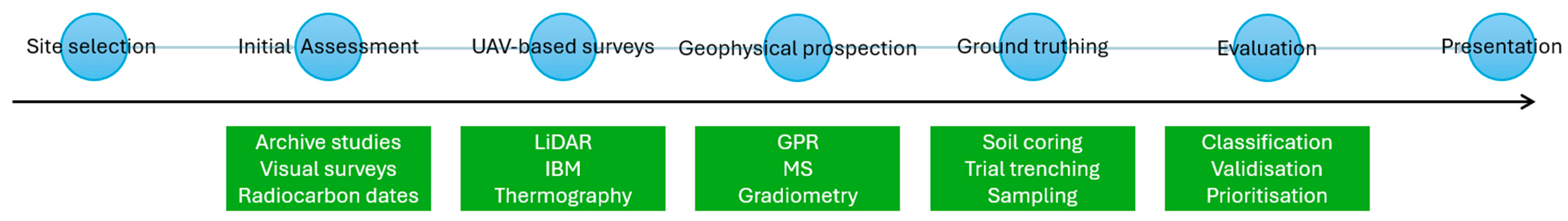
2. Materials and Methods
2.1. Light Detection and Ranging (LiDAR)
2.2. Image-Based Modelling (IBM)
2.3. Thermal Photography
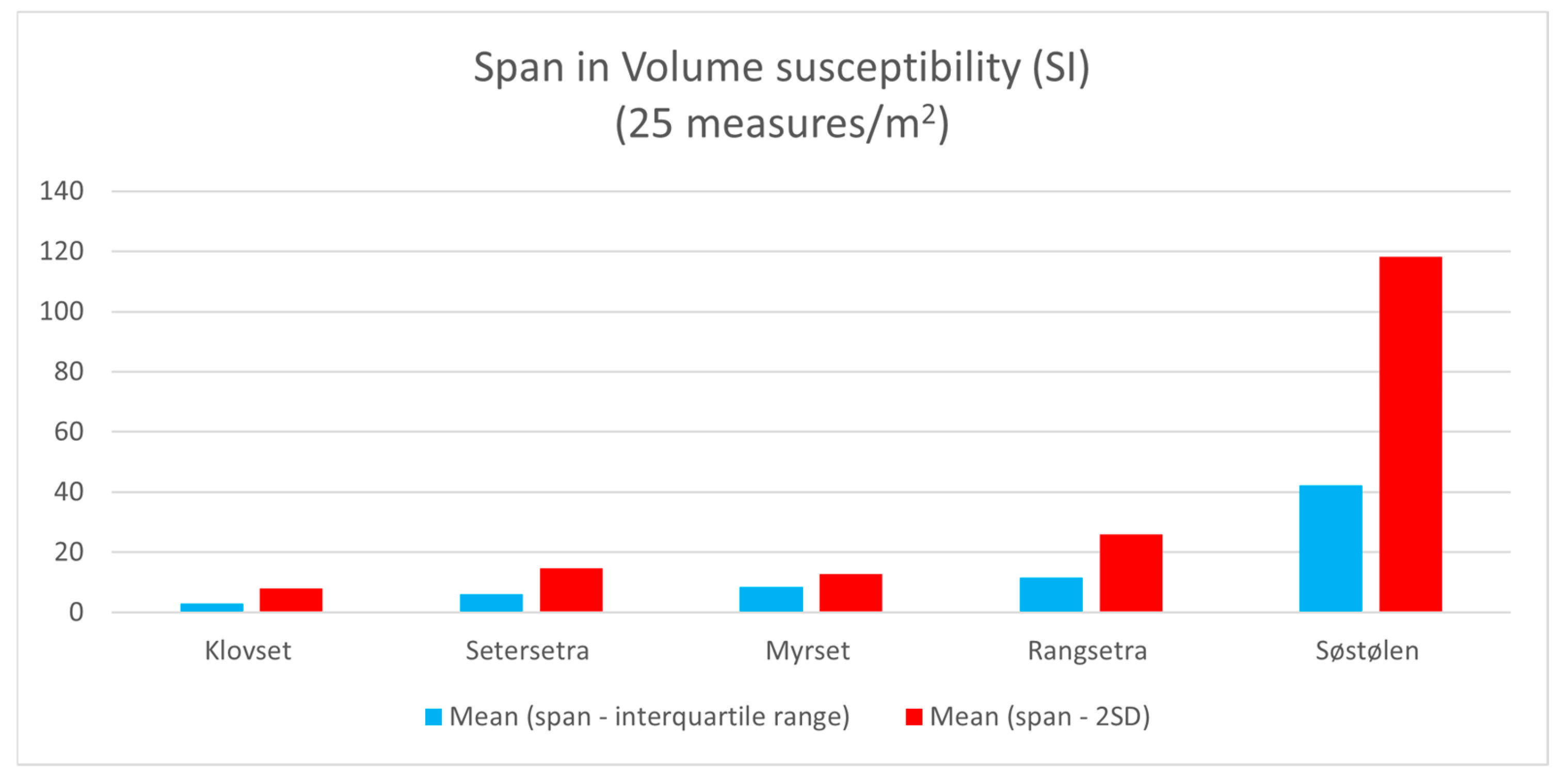
2.4. Topsoil Magnetic Susceptibility (MS) Survey
2.5. Fluxgate Gradiometer Survey
2.6. Ground Penetrating Radar (GPR)
2.7. Soil Coring
2.8. Manual Trial Trenching
3. Results
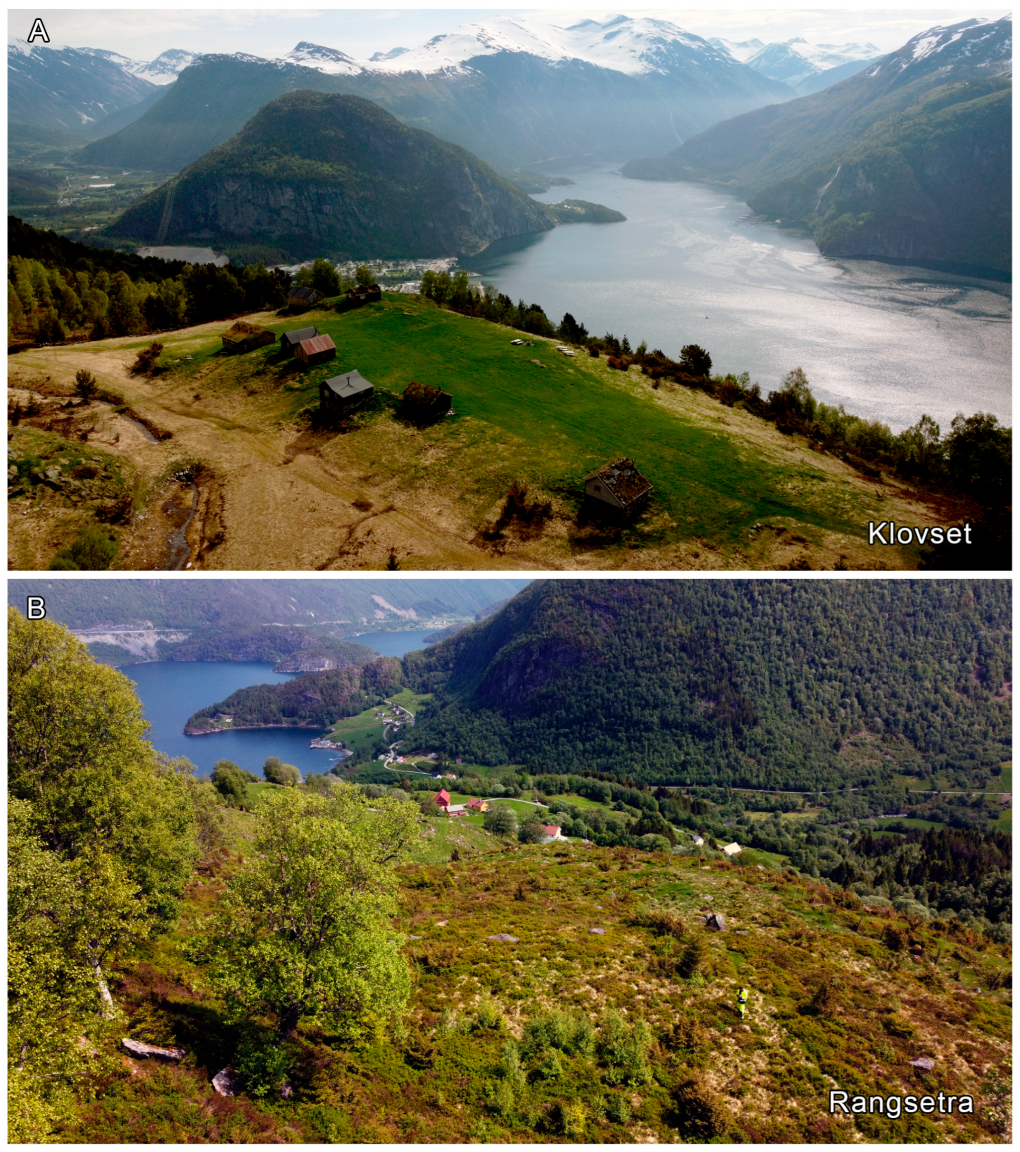
3.1. Klovset
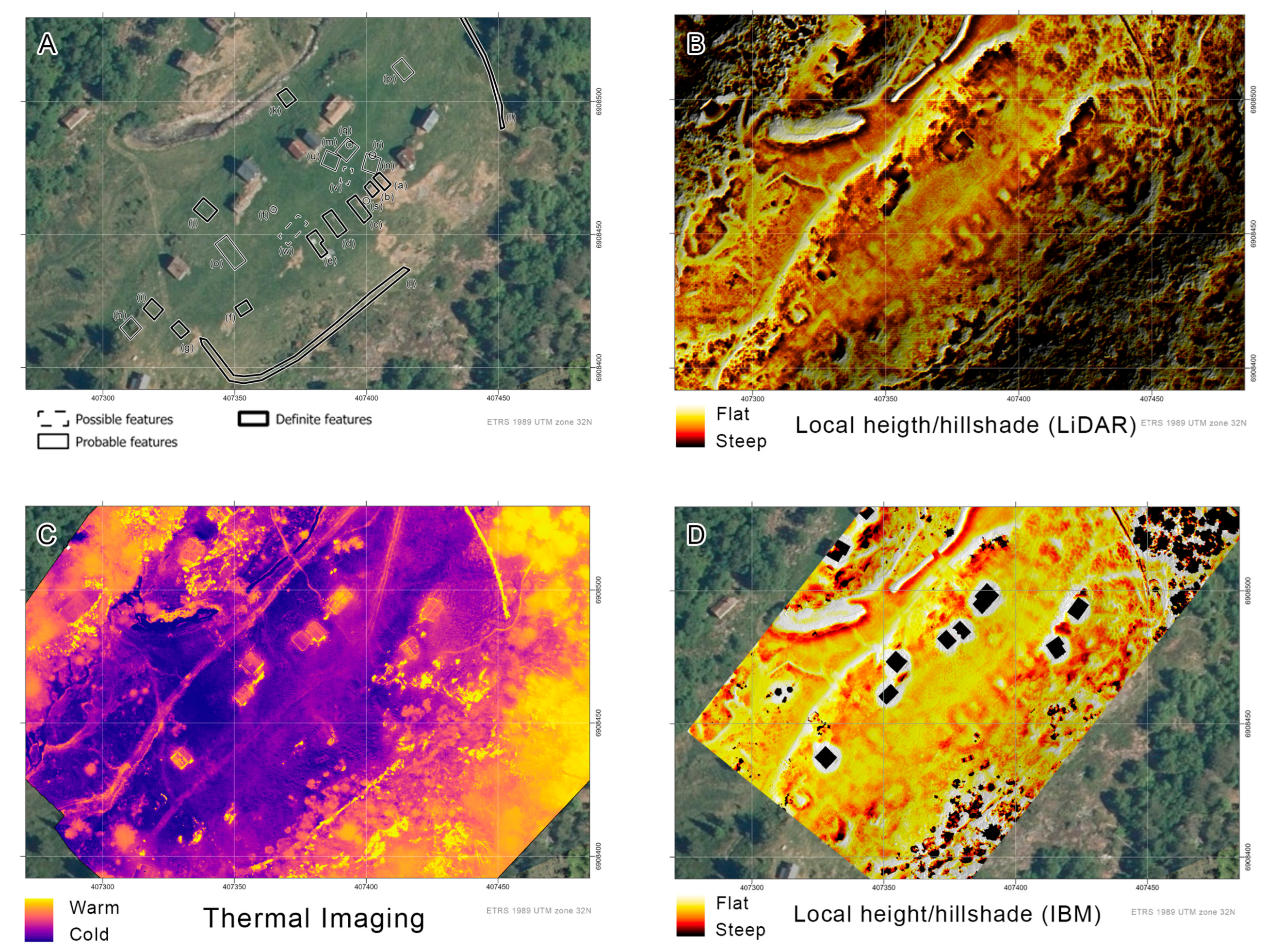
3.1.1. Aerial Survey
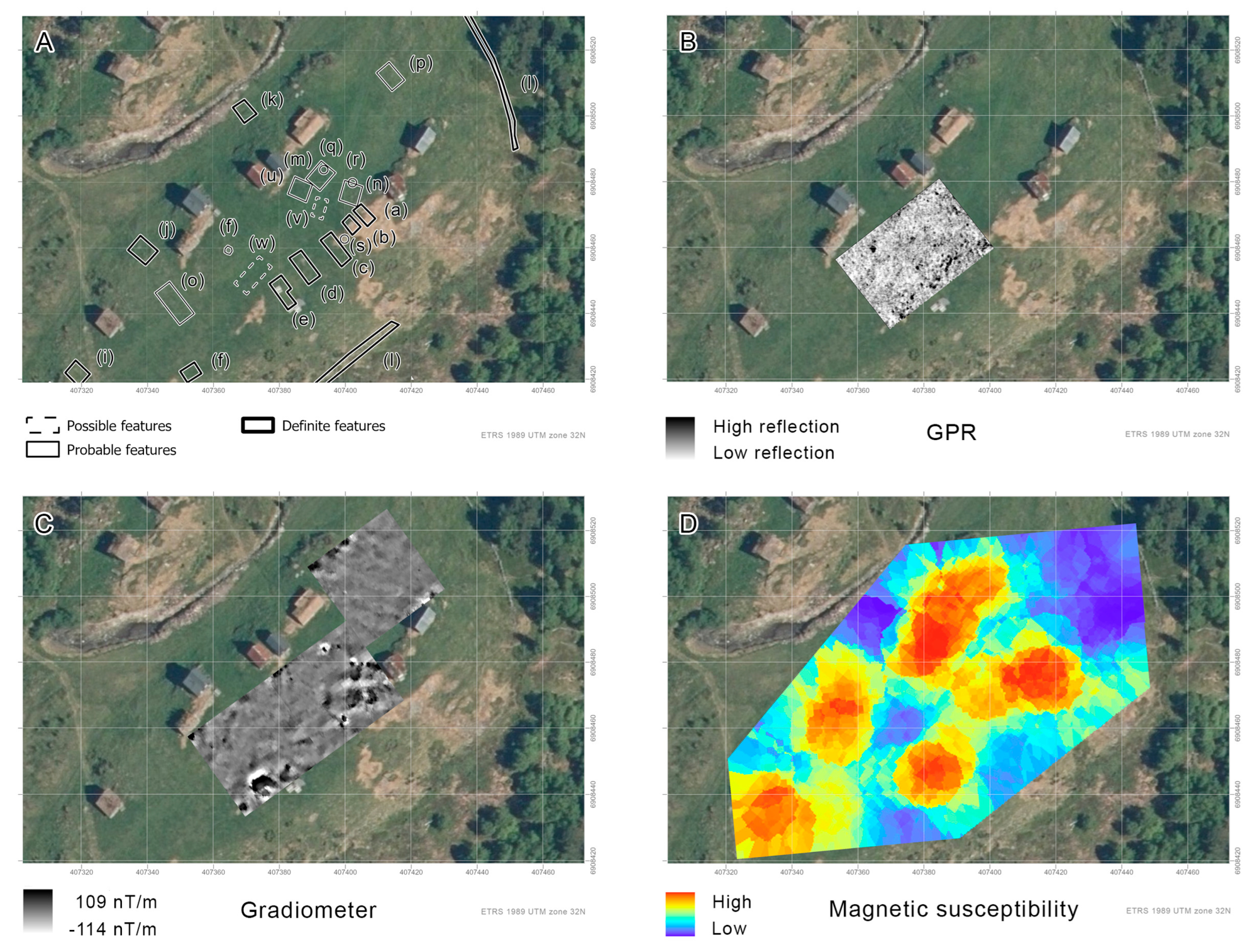
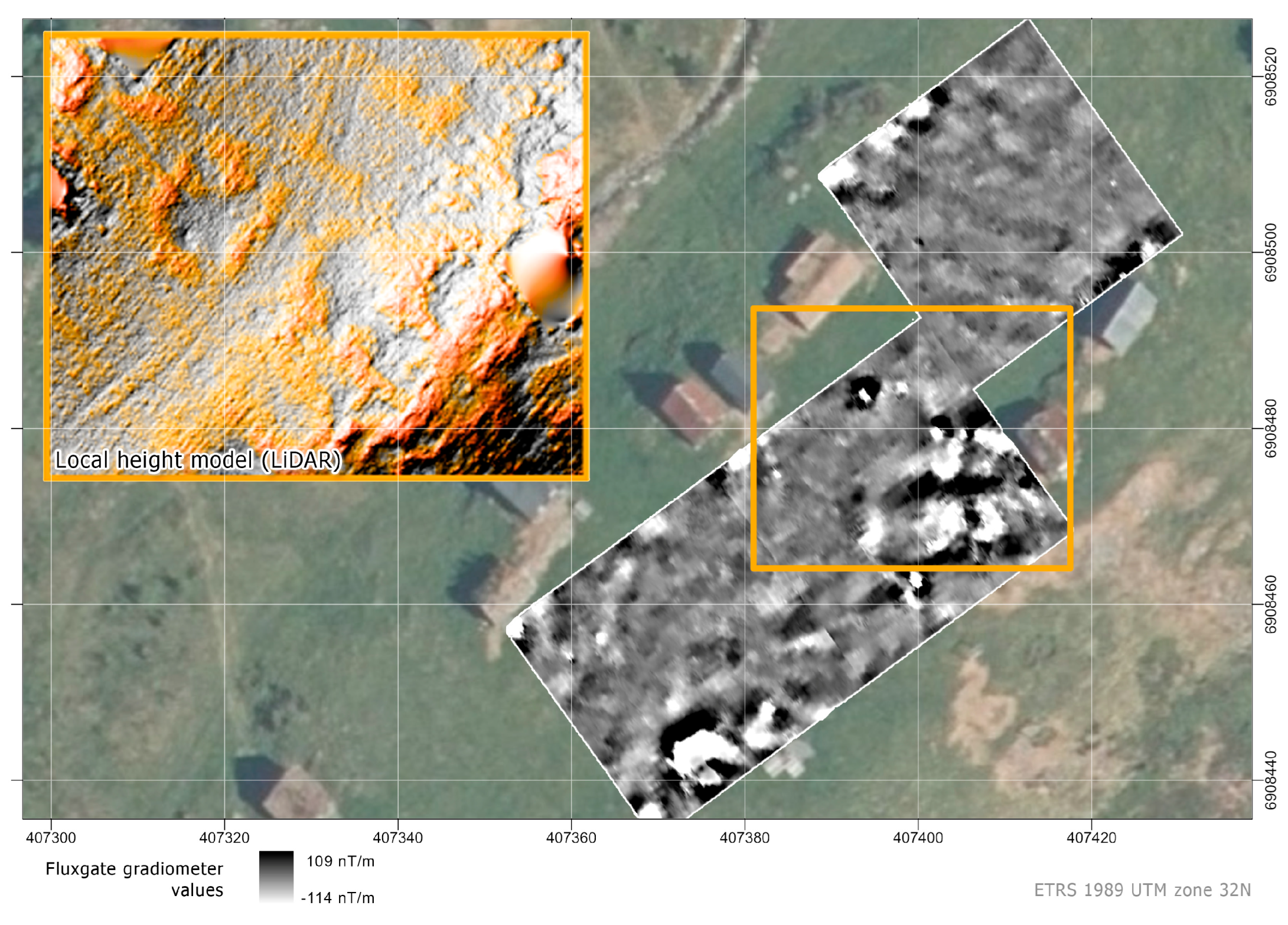
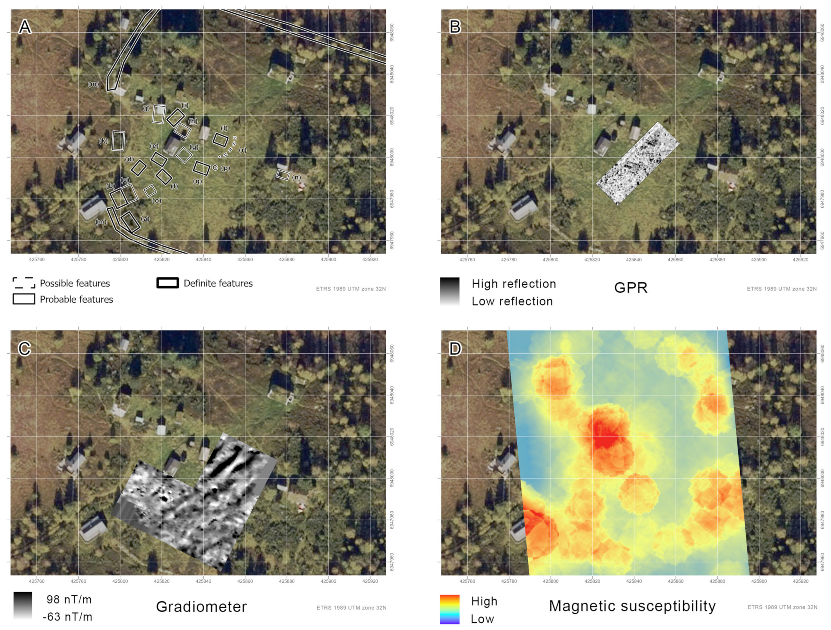
3.1.2. Geophysical Prospection
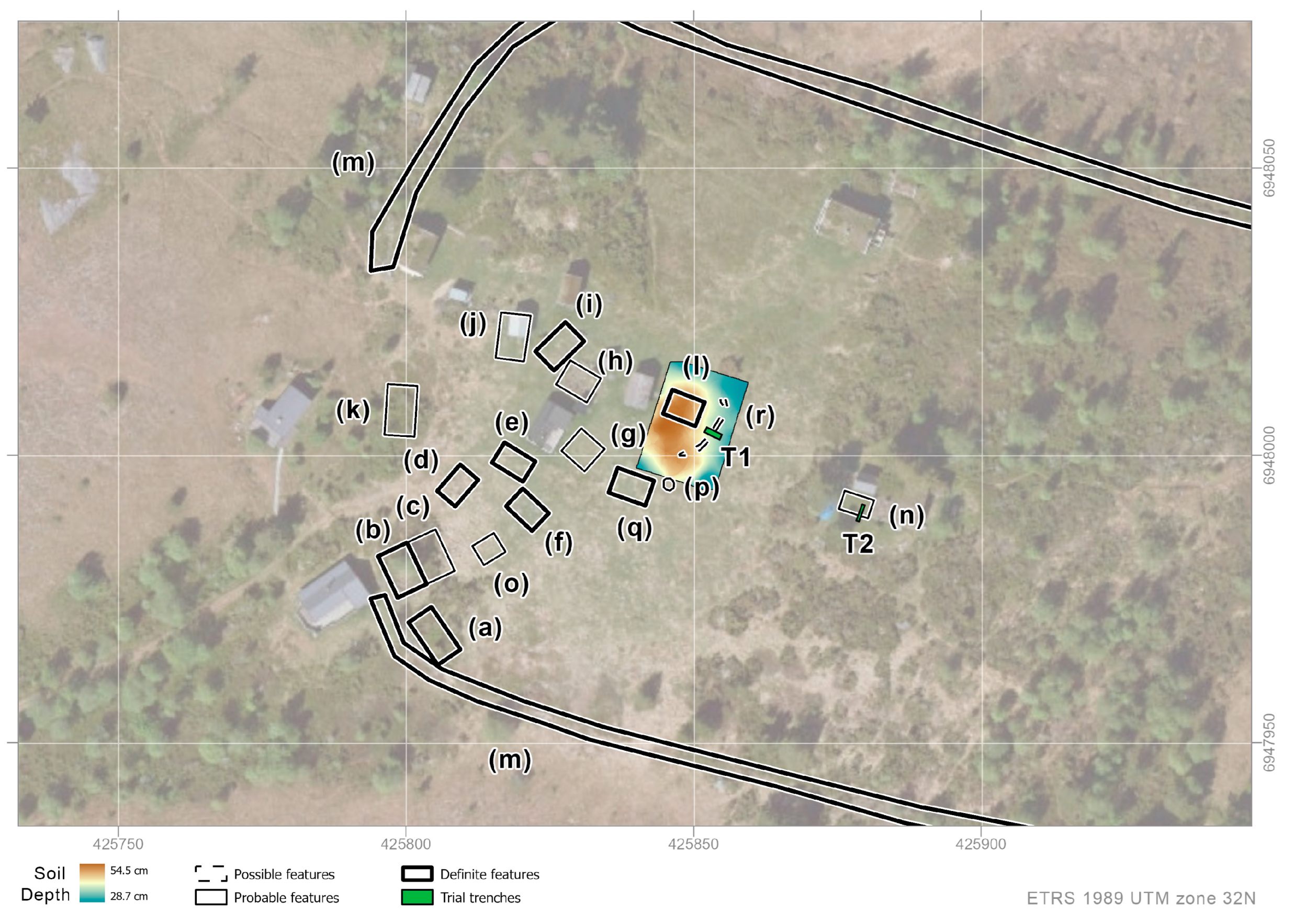
3.1.3. Soil Coring and Trial Trenching
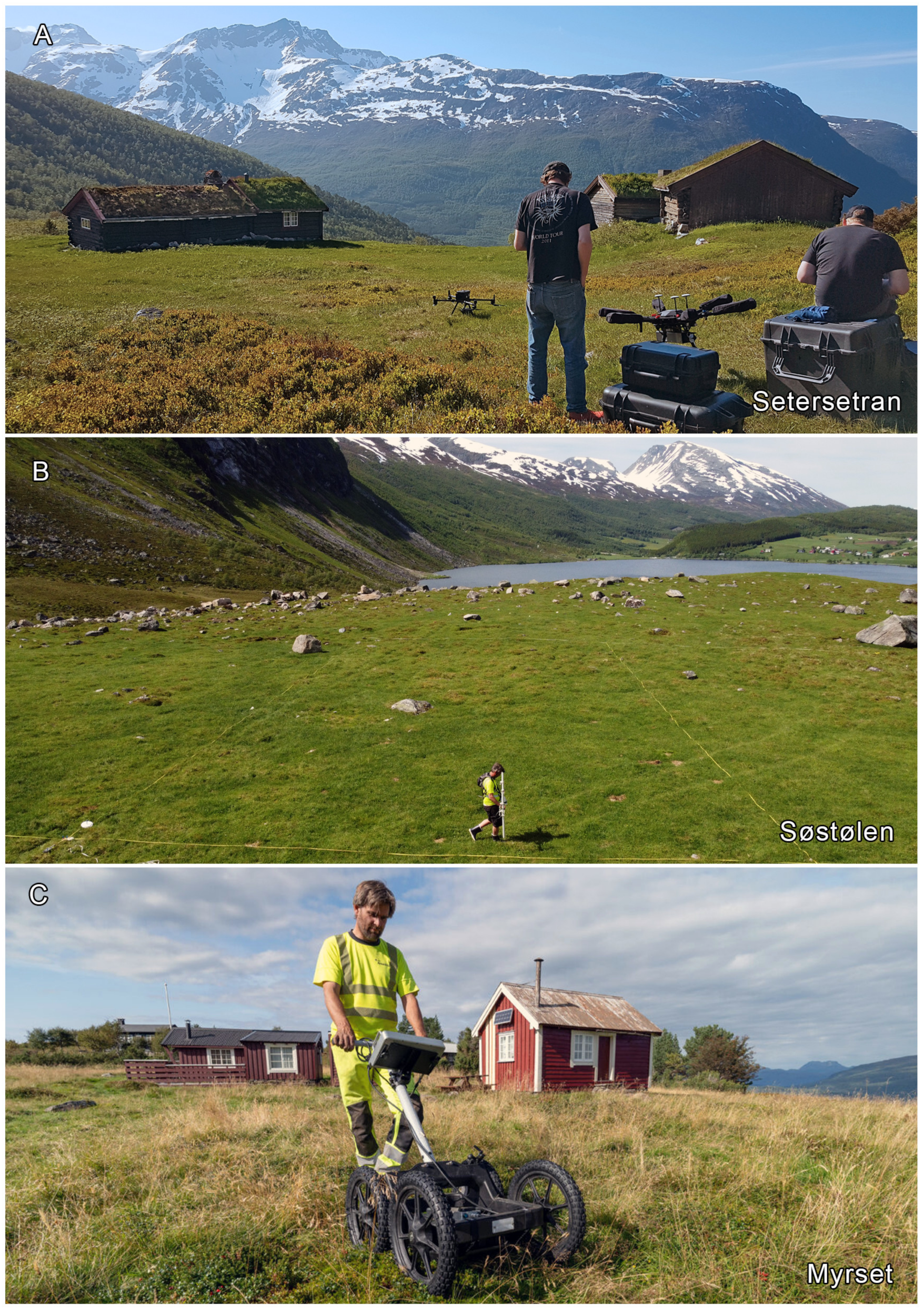
3.2. Setersetran
3.2.1. Aerial Survey
3.2.2. Geophysical Prospection
3.2.3. Soil Coring and Trial Trenching
3.3. Myrset
3.3.1. Aerial Survey
3.3.2. Geophysical Prospection
3.3.3. Soil Coring and Trial Trenching
3.4. Søstølen
3.4.1. Aerial Survey
3.4.2. Geophysical Prospection
3.4.3. Soil Coring and Trial Trenching
3.5. Rangsetra
3.5.1. Aerial Survey
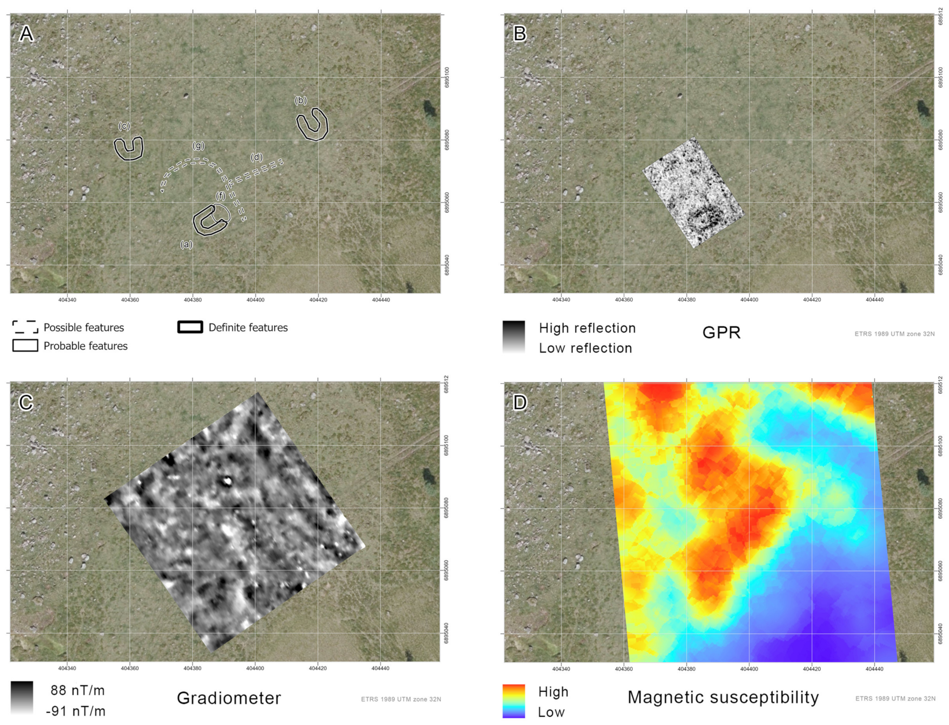
3.5.2. Geophysical Prospection
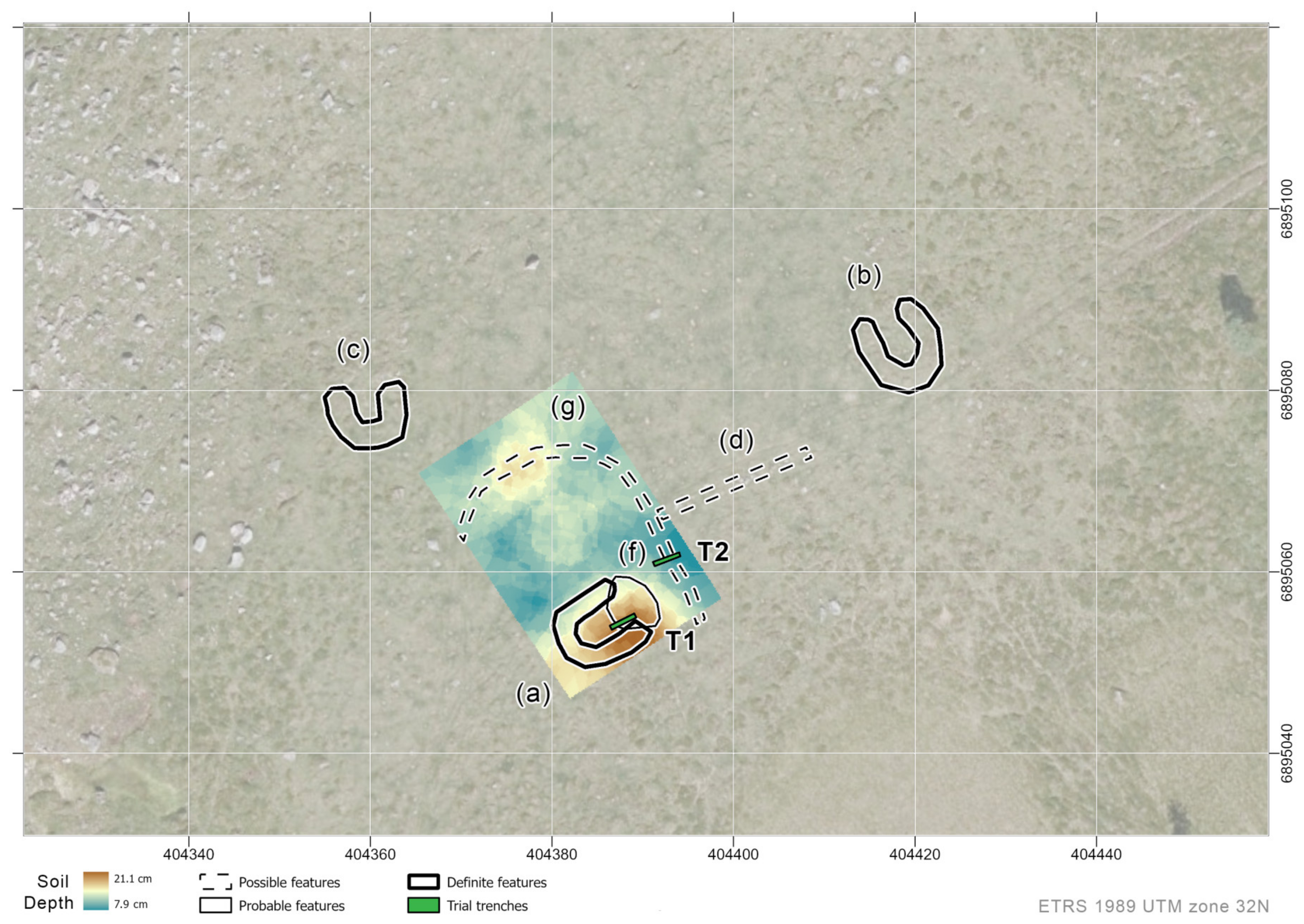
3.5.3. Soil Coring and Trial Trenching
4. Discussion
4.1. Practical Applicability—Access and Efficiency
4.2. Archaeological Results—Adequacy and Credibility
4.3. Implementation in Developer-Led Archaeology and Cultural Heritage Management Practices
5. Conclusions
Author Contributions
Funding
Data Availability Statement
Conflicts of Interest
Abbreviations
| AI | Artificial Intelligence |
| AR | Augmented Reality |
| ASCII | American Standard Code for Information Interchange |
| CPOS | Centimeter Positioning Service |
| GNSS | Global Navigation Satellite System |
| GPR | Ground Penetrating Radar |
| IBM | Image-Based Modelling |
| IMU | Inertial movement unit |
| LiDAR | Light Detection and Ranging |
| MS | Magnetic Susceptibility |
| NCHA | Norwegian Cultural Heritage Act |
| RTK | Real-Time Kinematic positioning |
| SfM | Structure from Motion |
| SI | International System of Units |
| SD | Standard derivation |
| UAV | Unmanned Aerial vehicle |
| VLOS | Visual Line Of Sight |
References
- Løken, T.; Pilø, L.; Hemdorff, O. Maskinell Flateavdekking og Utgravning av Forhistoriske Jordbruksboplasser—En Metodisk Innføring; AmS Varia 26; Archaeological Museum of Stavanger: Stavanger, Norway, 1996. [Google Scholar]
- Stamnes, A.A. The Application of Geophysical Methods in Norwegian Archaeology: A Study of the Status, Role and Potential of Geophysical Methods in Norwegian Archaeological Research and Cultural Heritage Management. Ph.D. Thesis, NTNU University Museum, Trondheim, Norway, 2016. Available online: https://ntnuopen.ntnu.no/ntnu-xmlui/handle/11250/2417713 (accessed on 26 February 2025).
- Gustavsen, L.; Stamnes, A.A.; Fretheim, S.E.; Gjerpe, L.E.; Nau, E. The Effectiveness of Large-Scale, High Resolution Ground-Penetrating Radar Surveys and Trial Trenching for Archaeological Site Evaluations—A Comparative Study form two Sites in Norway. Remote Sens. 2020, 12, 1408. [Google Scholar] [CrossRef]
- Norge i Bilder (Aerial Photos). Available online: http://norgeibilder.no (accessed on 26 February 2025).
- Høydedata (Elevation Data). Available online: http://hoydedata.no (accessed on 26 February 2025).
- Reinton, L. Sæterbruket i Noreg I. Sætertyper og Driftsformer; Aschehoug & Co: Oslo, Norway, 1955. [Google Scholar]
- Dahle, K. Støl, sel og seterstøl. Seterdrift gjennom 2000 år i Romsdal. Heimen 2007, 44, 343–358. [Google Scholar]
- Bjørgo, T. Iron Age house remains from mountain areas in inner Sogn, Western Norway. In Fra Funn til Samfunn. Jernalderstudier Tilegnet Bergljot Solberg på 70-Årsdagen; UBAS 1 Nordisk; Bergsvik, K.A., Engevik, A., Eds.; University of Bergen: Bergen, Norway, 2005; pp. 209–230. [Google Scholar]
- Bjørgo, T.; Kristoffersen, S.; Prescott, C. Arkeologiskeundersøkelser i Nyset-Steggjevassdragene 1981–1987; Arkeologiske rapporter 16; Historisk Museum: Bergen, Norway, 1992. [Google Scholar]
- Stene, K. I Randen av Taigaen—Bosetning og Ressursutnyttelse i Jernalder og Middelalder i Østerdalen; Gråfjellprosjektet; Portal/Museum of Cultural History: Oslo, Norway, 2014; Volume 4. [Google Scholar]
- Dahle, K. Tilblivelsen av setre som automatisk fredete kulturminner. Kvantitative og kvalitative tilnærminger til kulturminneforvaltningens håndtering av setre som arkeologiske kulturmiljø. Viking 2024, 87, 29–59. [Google Scholar]
- Stensgaard, K. Hvordan står det til på Setra? Registrering av Setermiljøer i Perioden 2009–2015; NIBIO Report 2017/88; NIBIO: Ås, Norway, 2018. [Google Scholar]
- Follestad, B.A. Løsmassekart over Møre og Romsdal Fylke: Beskrivelse; Skrifter 112; NGU/The Geological Survey of Norway: Trondheim, Norway, 1994. [Google Scholar]
- James, A.; James, M. Adding value to marine geophysics with visual interpretation. In Chartered Institute for Archaeologists, Yearbook and Directory; 2020; pp. 22–23. [Google Scholar]
- Opitz, R.S.; Herrmann, J.T. Recent Trends and Long-standing Problems in Archaeological Remote Sensing. J. Comput. Appl. Archaeol. 2018, 1, 19–41. [Google Scholar] [CrossRef]
- Doneus, M.; Briese, C. Digital Terrain Modelling for Archaeological Interpretation within Forested Areas using Full-Waveform Laser scanning. In VAST 2006: The 7th International Symposium on Virtual Reality, Archaeology and Intelligent Cultural Heritage; The Eurographics Association: Nicosia, Cyprus, 2006; pp. 155–162. [Google Scholar]
- Risbøl, O.; Gustavsen, L. LIDAR from drones employed for mapping archaeology—Potential, benefits and challenges. Archaeol. Prospect. 2018, 39, 103133. [Google Scholar] [CrossRef]
- Opitz, R.S.; Cowley, D.C. (Eds.) Interpreting Archaeological Topography: Airborne Laser Scanning, 3D Data and Ground Observation; Oxbow Books: Oxford, UK, 2013. [Google Scholar]
- Eidshaug, J.S.P.; Bjerck, H.B.; Breivik, H.M.; Risbøl, O.; Tivoli, A.M.; Zangrando, A.F.J. From earth to sky: Large-scale archaeological settlement patterns in southernmost South America based on ground surveys, UAV LiDAR, and open access satellite imagery. J. Isl. Coast. Archaeol. 2024, 1–40. [Google Scholar] [CrossRef]
- Vinci, G.; Vanzani, F.; Fontana, A.; Campana, S. LiDAR Applications in Archaeology: A Systematic Review. Archaeol. Prospect. 2024, 32, 81–101. [Google Scholar] [CrossRef]
- Gustavsen, L.; Paasche, K.; Risbøl, O. Arkeologiske Undersøkelser. Vurdering av Nyere Avanserte Arkeologiske Registreringsmetoder; Norwegian Public Roads Administration: Oslo, Norway, 2013. [Google Scholar]
- Trier, Ø.D.; Reksten, J.H.; Løseth, K. Automated mapping of cultural heritage in Norway from airborne lidar data using faster R-CNN. Int. J. Appl. Earth Obs. Geoinf. 2021, 95, 102241. [Google Scholar] [CrossRef]
- Kokalj, Ž.; Hesse, R. Airborne Laser Scanning Raster Data Visualization: A Guide to Good Practice; Založba ZRC: Ljubljana, Slovenia, 2017. [Google Scholar]
- Kokalj, Ž.; Somrak, M. Why Not a Single Image? Combining Visualizations to Facilitate Fieldwork and On-Screen Mapping. Remote Sens. 2019, 11, 747. [Google Scholar] [CrossRef]
- Forsyth, D.A.; Ponce, J. Computer Vision: A Modern Approach; Prentice Hall: Upper Saddle River, NJ, USA, 2012. [Google Scholar]
- Szelinski, R. Computer Vision: Algorithms and Applications; Springer: London, UK; Dordrecht, The Netherlands; Heidelberg, Germany; New York, NY, USA, 2010. [Google Scholar]
- Remondino, F.; Campana, S. (Eds.) 3D Recording and Modelling in Archaeology and Cultural Heritage—Theory and Best Practices; Bar International Series 2598; Archaeopress: Oxford, UK, 2014. [Google Scholar]
- Historic England. Photogrammetric Applications for Cultural Heritage. Guidance for Good Practice. Historic England, Swindon, UK. 2017. Available online: https://historicengland.org.uk/images-books/publications/photogrammetric-applications-for-cultural-heritage/ (accessed on 3 February 2025).
- Gigamesh. Available online: https://www.gigamesh.eu/downloads (accessed on 26 February 2025).
- Ammer, K.; Ring, F. The Thermal Human Body: A Practical Guide to Thermal Imaging; Jenny Stanford Publishing: Singapore, 2019. [Google Scholar]
- Barbara, J.; Chudoba, T.; Skarzynski, P. Application of Thermal Imaging in Archaeological Prospection—A Case Study. Acta Geophysica 2009, 57, 740–753. [Google Scholar]
- Casana, J.; Wiewel, A.; Cool, A.; Hill, A.C.; Fisher, K.D.; Laugier, E.J. Archaeological Aerial Thermography in Theory and Practice. Adv. Archaeol. Pract. 2017, 5, 310–327. [Google Scholar] [CrossRef]
- Dearing, J. Environmental Magnetic Susceptibility: Using the Bartingston MS2 System; Chi Publishing: Keniloworth, UK, 1999. [Google Scholar]
- Dalan, R.A. A review of the Role of Magnetic Susceptibility in Archaeogeophysical Studies in the USA: Recent Developments and Prospects. Archaeol. Prospect. 2008, 13, 1–31. [Google Scholar]
- Solli, B.; Stamnes, A.A. Geofysiske undersøkelser av kirker, kirketufter og svartjord på Veøya i Romsdal. Viking 2013, 76, 181–202. [Google Scholar]
- Stamnes, A.A.; Risbøl, O.; Stenvik, L.F. Investigating Early Iron Production by Modern Remote Sensing Technologies; Skrifter 2:2019; The Royal Norwegian Society of Sciences and Letters: Trondheim, Norway, 2019. [Google Scholar]
- Dahle, K.; Stamnes, A.A. Their smaar koupstader—Omfang, struktur og oppkomst. Nye arkeologiske og geofysiske undersøkelser på Veøya. In Kjøpstaden på veøya. Middelalderbyen som Forsvant; VITARK 12; Dahle, K., Nytun, A., Langnes, M., Rundberget, B., Eds.; NTNU University Museum/Museumsforlaget: Trondheim, Norway, 2024; pp. 68–85. [Google Scholar]
- Stamnes, A.A. Developing a Sequential Geophysical Survey Design for Norwegian Iron Age Settlements. Master’s Thesis, University of Bradford, Bradford, UK, 2010. [Google Scholar]
- Fredriksen, C.; Stamnes, A.A. Geofysiske Undersøkelser og Sosialt Metallsøk på Løykja, Sunndal Kommune, Møre og Romsdal; Archaeological report 2019:23; NTNU University Museum: Trondheim, Norway, 2019. [Google Scholar]
- Stamnes, A.A. Georadar avdekker fortidsminner. Spor 2011, 1, 30–33. [Google Scholar]
- Lecoanet, H.; Lévêque, F.; Segura, S. Magnetic Susceptibility in environmental applications: Comparisons of field probes. Phys. Earth Planet. Inter. 1999, 115, 191–204. [Google Scholar] [CrossRef]
- Hargrave, M. Ground Truthing the Results of Geophysical Surveys. In Remote Sensing in Archaeology: An Explicitly North American Perspective; Johnson, J.K., Ed.; University of Alabama Press: Tuscaloosa, AL, USA, 2006; pp. 269–304. [Google Scholar]
- Aspinall, A.; Gaffney, C.; Schmidt, A. Magnetometry for Archaeologists. Geophysical Methods for Archaeology; Alta Mira Press: Lanham, MD, USA, 2009. [Google Scholar]
- Conyers, L.B. Ground-Penetrating Radar for Archaeology, 4th ed.; Rowman & Littlefield Publishers: Lanham, MD, USA, 2023. [Google Scholar]
- Goodman, D.; Piro, S. GPR Remote Sensing in Archaeology; Springer: Berlin/Heidelberg, Germany, 2013; Volume 9. [Google Scholar]
- Stein, J.K. Coring Archaeological Sites. Am. Antiq. 1986, 51, 505–527. [Google Scholar] [CrossRef]
- Marken, D.; Ricker, M.C.; Austin, R. Combining Survey, Soil Coring, and GIS Methods to Improve Reservoir Capacity Estimates in the Maya Lowlands. Adv. Archaeol. Pract. 2022, 10, 187–199. [Google Scholar] [CrossRef]
- Petterson, S. From written sources to archaeological remains—Medieval shielings in central Scandinavia. In Historical Archaeologies of Transhumance across Europe; Themes in Contemporary Archaeology; Costello, E., Svensson, E., Eds.; Routledge: London, UK; New York, NY, USA, 2018; pp. 29–41. [Google Scholar]
- Olsen, M. Ættegård og Helligdom. Norske Stedsnavn, Sosial og Religionshistorisk Belyst; Aschehoug & Co.: Oslo, Norway, 1926. [Google Scholar]
- Dahle, K. Ny Fritidshytte—Klovset, Unpublished Survey Report; Møre & Romsdal, Norway, 2016.
- Dahle, K. Norm og Praksis. Bruk og Forvaltning av Utmark i Midtre Romsdal i et Langtidsperspektiv. Master’s Thesis, University of Bergen, Bergen, Norway, 2005. Available online: https://bora.uib.no/bora-xmlui/handle/1956/2296 (accessed on 26 February 2025).
- Dahle, K. Tilbygg, Myrset, Unpublished Survey Report; Møre & Romsdal, Norway, 2014.
- Sauvage, R. Utgraving av Kulturlag og Jernvinneanlegg på Myrsetseteren; Archaeological report 2018:1; NTNU University Museum: Trondheim, Norway, 2018. [Google Scholar]
- Johnston, A. Indreeide i Norddal, Korsmyra i Stranda, Unpublished survey report; Møre & Romsdal, Norway, 2015.
- Årviknes, P. Volda-soga III. Garder og slekter; Volda trykkeri: Volda, Norway, 1973. [Google Scholar]
- Sortland, S. 420 kV Ørskog–Fardal, Unpublished survey report; Møre & Romsdal, Norway, 2010.
- Schmidt, A.; Marshall, A. Impact of resolution on the interpretation of archaeological prospection data. In Archaeological Sciences 1995; Oxbow Monograph in, archaeology; Sinclair, A.G.M., Gowlett, E., Eds.; Oxford Bows: Oxford, UK, 1997; pp. 343–348. [Google Scholar]
- Kulturminneloven (Norwegian Cultural Heritage Act). Available online: https://lovdata.no/dokument/NLE/lov/1978-06-09-50 (accessed on 26 February 2025).


| Site and Method | Area (km2) | Aligned Images | Points/ Vertices (Millions) | Point Spacing (m) | Point Density | Flight Pattern | GSD (cm) |
|---|---|---|---|---|---|---|---|
| Klovset | |||||||
| LiDAR | 1.070 | - | 30.31 | 0.111 | 81.2 | Cross grid | - |
| IBM | 0.053 | 1047 | 102.49 | 0.021 | 2178 | Lines | 13.71 |
| Thermal | 0.047 | 962 | 7.00 | 0.082 | 93.2 | Lines | 5.00 |
| Setersetran | |||||||
| LiDAR | 1.893 | - | 19.58 | 0.109 | 84.2 | Cross grid | - |
| IBM | 0.020 | 1329 | 86.06 | 0.015 | 4303 | Lines | 6.86 |
| Thermal | 0.018 | 1394 | 7.28 | 0.050 | 440.4 | Lines | 3.46 |
| Myrset | |||||||
| LiDAR | 1.449 | - | 29.71 | 0.110 | 82.6 | Cross grid | - |
| IBM | 0.023 | 1151 | 94.06 | 0.015 | 4090 | Lines | 8.22 |
| Thermal | 0.022 | 1122 | 6.67 | 0.057 | 267.3 | Lines | 3.67 |
| Søstølen | |||||||
| LiDAR | 0.678 | - | 39.86 | 0.101 | 98.0 | Cross grid | - |
| IBM | 0.050 | 906 | 180.49 | 0.016 | 3609 | Lines | 13.71 |
| Thermal | 0.032 | 721 | 8.47 | 0.061 | 361.1 | Lines | 3.19 |
| Rangsetra | |||||||
| LiDAR | 1.635 | - | 6.07 | 0.157 | 40.6 | Lines | - |
| IBM | 0.032 | 582 | 63.18 | 0.022 | 1973 | Lines | 10.97 |
| Thermal | 0.015 | 543 | 3.42 | 0.066 | 153.2 | Lines | 4.05 |
| Site (Trench) | Mean SI Span (IQR) | Mean SI Span (SD) | Outliers (n) |
|---|---|---|---|
| Klovset (T3) | 2.00 | 6.67 | 1 |
| Klovset (T2) | 4.00 | 9.33 | 2 |
| Setersetran (T1) | 5.00 | 12.67 | 2 |
| Setersetran (T0) | 7.17 | 16.67 | 4 |
| Myrset (T1) | 8.67 | 5.67 | 1 |
| Myrset (T2) | 4.67 | 13.00 | 7 |
| Myrset (T0) | 12.00 | 20.00 | 4 |
| Rangsetra (T1) | 11.50 | 26.00 | 4 |
| Søstølen (T2) | 22.33 | 56.67 | 0 |
| Søstølen (T1) | 62.25 | 180.00 | 3 |
| Site | LiDAR | Thermal | IBM | MS | Gradiom. | GPR | Coring |
|---|---|---|---|---|---|---|---|
| Klovset | 40 * | 3.20 | 3.20 | 0.86 | 0.27 | 0.11 | 0.09 |
| Setersetran | 30 * | 1.51 | 1.51 | 1.12 | 0.36 | 0.04 * | 0.10 |
| Myrset | 50 * | 1.62 | 1.62 | 1.42 | 0.27 | 0.06 | 0.04 |
| Søstølen | 30 * | 3.05 | 3.05 | 0.89 | 0.36 | 0.06 | 0.06 |
| Rangsetra | 30 * | 1.58 | 1.58 | 0.23 * | 0.09 | - | 0.04 |
Disclaimer/Publisher’s Note: The statements, opinions and data contained in all publications are solely those of the individual author(s) and contributor(s) and not of MDPI and/or the editor(s). MDPI and/or the editor(s) disclaim responsibility for any injury to people or property resulting from any ideas, methods, instructions or products referred to in the content. |
© 2025 by the authors. Licensee MDPI, Basel, Switzerland. This article is an open access article distributed under the terms and conditions of the Creative Commons Attribution (CC BY) license (https://creativecommons.org/licenses/by/4.0/).
Share and Cite
Dahle, K.; Solem, D.-Ø.E.; Gran, M.M.; Stamnes, A.A. Making the Invisible Visible: The Applicability and Potential of Non-Invasive Methods in Pastoral Mountain Landscapes—New Results from Aerial Surveys and Geophysical Prospection at Shielings Across Møre and Romsdal, Norway. Remote Sens. 2025, 17, 1281. https://doi.org/10.3390/rs17071281
Dahle K, Solem D-ØE, Gran MM, Stamnes AA. Making the Invisible Visible: The Applicability and Potential of Non-Invasive Methods in Pastoral Mountain Landscapes—New Results from Aerial Surveys and Geophysical Prospection at Shielings Across Møre and Romsdal, Norway. Remote Sensing. 2025; 17(7):1281. https://doi.org/10.3390/rs17071281
Chicago/Turabian StyleDahle, Kristoffer, Dag-Øyvind Engtrø Solem, Magnar Mojaren Gran, and Arne Anderson Stamnes. 2025. "Making the Invisible Visible: The Applicability and Potential of Non-Invasive Methods in Pastoral Mountain Landscapes—New Results from Aerial Surveys and Geophysical Prospection at Shielings Across Møre and Romsdal, Norway" Remote Sensing 17, no. 7: 1281. https://doi.org/10.3390/rs17071281
APA StyleDahle, K., Solem, D.-Ø. E., Gran, M. M., & Stamnes, A. A. (2025). Making the Invisible Visible: The Applicability and Potential of Non-Invasive Methods in Pastoral Mountain Landscapes—New Results from Aerial Surveys and Geophysical Prospection at Shielings Across Møre and Romsdal, Norway. Remote Sensing, 17(7), 1281. https://doi.org/10.3390/rs17071281