Article

Remote Sensing Reveals Multidecadal Trends in Coral Cover at Heron Reef, Australia

by
David E. Carrasco Rivera
1,*,
Faye F. Diederiks
1,
Nicholas M. Hammerman
1,
Timothy Staples
2,
Eva Kovacs
1,
Kathryn Markey
3 and
Chris M. Roelfsema
1
1
Marine Ecosystem Monitoring Lab, School of The Environment, University of Queensland, Brisbane, QLD 4072, Australia
2
School of The Environment, University of Queensland, Brisbane, QLD 4072, Australia
3
Earth Observation Research Centre, School of The Environment, University of Queensland, Brisbane, QLD 4072, Australia
*
Author to whom correspondence should be addressed.
Remote Sens. 2025, 17(7), 1286; https://doi.org/10.3390/rs17071286
Submission received: 24 February 2025 / Revised: 20 March 2025 / Accepted: 1 April 2025 / Published: 3 April 2025
(This article belongs to the Section Ocean Remote Sensing)

Abstract

:
Coral reefs are experiencing increasing disturbance regimes. The influence these disturbances have on coral reef health is traditionally captured through field-based monitoring, representing a very small reef area (<1%). Satellite-based observations offer the ability to up-scale the spatial extent of monitoring efforts to larger reef areas, providing valuable insights into benthic trajectories through time. Our aim was to demonstrate a repeatable benthic habitat mapping approach integrating field and satellite data acquired annually over 21 years. With this dataset, we analyzed the trends in benthic composition for a shallow platform reef: Heron Reef, Australia. Annual benthic habitat maps were created for the period of 2002 to 2023, using a random forest classifier and object-based contextual editing, with annual in situ benthic data derived from geolocated photoquadrats and coincident high-spatial-resolution (2–5 m pixel size) multi-spectral satellite imagery. Field data that were not used for calibration were used to conduct accuracy assessments. The results demonstrated the capability of remote sensing to map the time series of benthic habitats with overall accuracies between 59 and 81%. We identified various ecological trajectories for the benthic types, such as decline and recovery, over time and space. These trajectories were derived from satellite data and compared with those from the field data. Remote sensing offered valuable insights at both reef and within-reef scales (i.e., geomorphic zones), complementing percentage cover data with precise surface area metrics. We demonstrated that monitoring benthic trajectories at the reef scale every 2 to 3 years effectively captured ecological trends, which is crucial for balancing resource allocation.

1. Introduction

Coral reefs provide a wealth of ecosystem services, contributing significantly to local economies worldwide. Yet, coral reefs are highly threatened by localized human-driven stressors and by global climate-change-driven disturbance events [1,2,3,4]. Changes in benthic composition can transform habitat complexity and can occur over different temporal (e.g., months or years) and spatial (e.g., within-geomorphic zones, within-reef, whole-reef, or between-reef) resolutions, which can affect ecological processes and ecosystem services [5,6,7].
Changes in coral cover can act as an indicator of trajectories of recovery and/or decline, providing insights into the overall health of coral reefs, while also being easily measured in the field [8]. Even so, studies of ecosystem monitoring generally use field data representing less than 1% of the surface area of a reef [9,10]. These studies of compositional change over time and space are also generally conducted after a singular disturbance event (i.e., bleaching, disease outbreak, etc.) [11,12,13]. Ultimately, this has led to a spatially and temporally constrained understanding of long-term trends in coral dynamics.
Cycles of disturbance and recovery operate at varied temporal scales, in which acute disturbances can reduce coral cover within days (e.g., cyclones), across monthly to annual scales (e.g., bleaching), and across decadal timeframes (e.g., ocean acidification) [14]. Contrastingly, reef recovery tends to be a slower, potentially decadal process and can take longer than what most ecological field studies have the ability to monitor [15,16]. Coral growth can be as little as 4–12 mm/year [17] and result in a total reef accretion of only a few centimeters per year, a number that can vary dramatically depending on depth, hydrodynamics, and substrate type [18].
Longer and spatially explicit studies are crucial to disentangle natural changes in community composition and stochastic effects from the impact of disturbances [8,19]. Remote sensing image data add value to monitoring programs, expanding spatial and temporal scales beyond what is covered by field data. By integrating annotated georeferenced field data with satellite imagery via pixel- and/or object-based image analysis (OBIA), it could be possible to develop time-series analyses that identify the trajectories of and changes in entire reef systems [20,21]. The recent accessibility of global coverage satellite imagery such as Landsat (30 m resolution), Sentinel (10 m), and Planet (3 m), has provided the ability to monitor changes in various land ecosystems at the global scale [22,23]. Thus far, changes in coral reef composition have been mapped over a period of less than 10 years using coarse-scale sensors and at coarser time intervals [24,25,26].
The submerged and remote nature of coral reefs causes increases in the cost of field monitoring, and it limits the thematic level that can be identified via remote sensing. While remote sensing can differentiate habitat types (coral, algae, seagrass, sand, and rubble) [20], it does not allow for the identification of finer details such as coral morphologies or species. However, accurate and reliable benthic classification in coral reefs using remote sensing has provided ecologically relevant spatial information to guide management and policy-making processes [27]. For this information to be accurate and reliable, field data must (1) be collected around the same time as the acquisition of the satellite imagery [28] and (2) be both representative of the habitat composition and of sufficient detail to be incorporated into remote sensing processes [29]. Additionally, while images from the Landsat (30 m) and Sentinel (10 m) satellites have demonstrated their ability to map coral habitats [30,31], these products often overestimate the accuracy of habitat classifications due to the large difference between the sensor resolution and the fine-scale changes in coral habitats. Therefore, satellite imagery needs to be of a suitable resolution (0.5–4 m) to differentiate benthic types over time and space, representing the high levels of heterogeneity of coral reefs [32,33].
By applying empirical knowledge derived from field data and local expertise, remote sensing can aid in identifying different trends at the reef scale and even at smaller scales such as the within-reef scale (i.e., geomorphic zones such as reef slopes, reef crests, and reef flats) [34]. Developing whole-reef-scale spatially explicit time-series analyses that incorporate multiple stressors (e.g., bleaching events, disease outbreaks, and cyclones) is crucial for understanding how these events affect entire coral assemblages and their resistance and resilience to further disturbances. Such robust analyses enable managers to translate spatiotemporal data into insights about ecological processes and ecosystem services, ultimately informing management, conservation, and restoration strategies [35].
Here, we aimed to (1) build a repeatable, accurate, and reliable field and satellite data-based benthic habitat mapping approach, (2) test the performance of this approach in detecting ecologically relevant changes in benthic coral reef composition over decadal timescales, and (3) determine the temporal grain at which these changes can be reliably detected via remote sensing. To develop this method, we used a comprehensive field and image dataset from Heron Reef, Southern Great Barrier Reef, Australia. This dataset spans over two decades (from 2002 to 2023 at the time of writing), with annual field observations of benthic composition across different reef zones [36], and coincides with high-spatial-resolution multi-spectral satellite imagery.

2. Materials and Methods
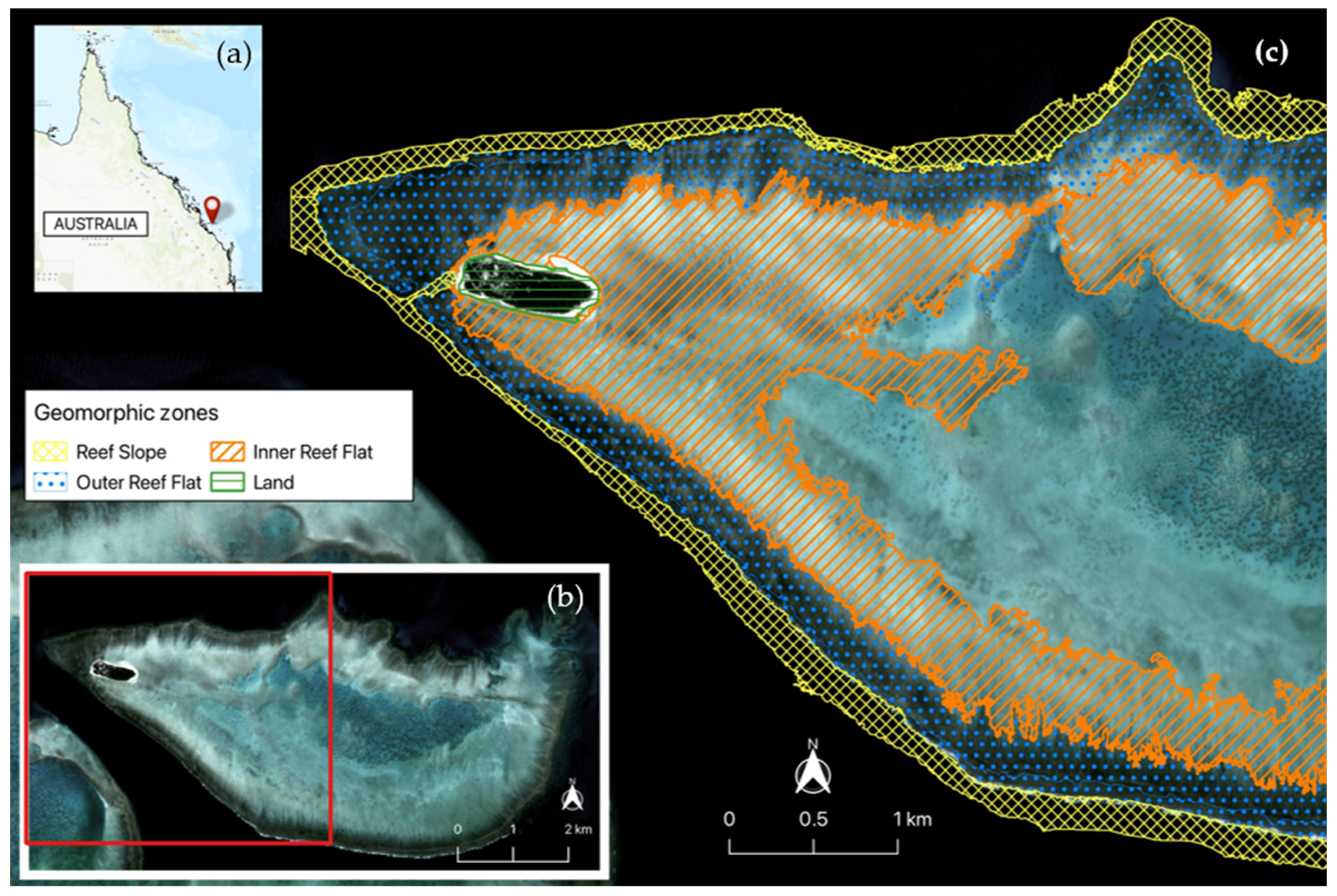
The methodology for this work contained the following steps: (1) categorize benthic composition in field data, (2) pre-process satellite imagery, (3) apply Random Forest (RF) classification of satellite imagery using field data, (4) validate model performance, and (5) analyze trends in benthic composition through time (Figure 1).

2.1. Study Site

Heron Reef is a platform reef (28 km2) located within the Capricorn Bunker Group in the Southern Great Barrier Reef (GBR), Australia (Figure 2). Heron has been studied extensively for various research purposes through the presence of the Heron Island Research Station. This includes previous and on-going remote sensing research supported by the long-term time-series dataset [37,38,39,40,41,42,43]. The reef itself has been subject to various impacts such as minor coral bleaching, cyclones, storms, and disease outbreaks [44], making this a relevant area for the development of this current study.

2.2. Datasets

This study focused on the region of the reef with the most extensive and consistent field and satellite data records for the entire time series. This ensured that we could produce the most accurate and repeatable mapping approach that would result in representative maps. This area, of approximately 3.44 km2, spans the western section of the reef, covering the outer reef flat and reef slope geomorphic zones, which are primarily composed of hard substrate (Figure 2c and Figure 3) [46,47]. The other geomorphic zones of the reef (i.e., inner reef flat and lagoons) were not mapped due to their predominant sand cover and the lack of consistent field data throughout the time series.

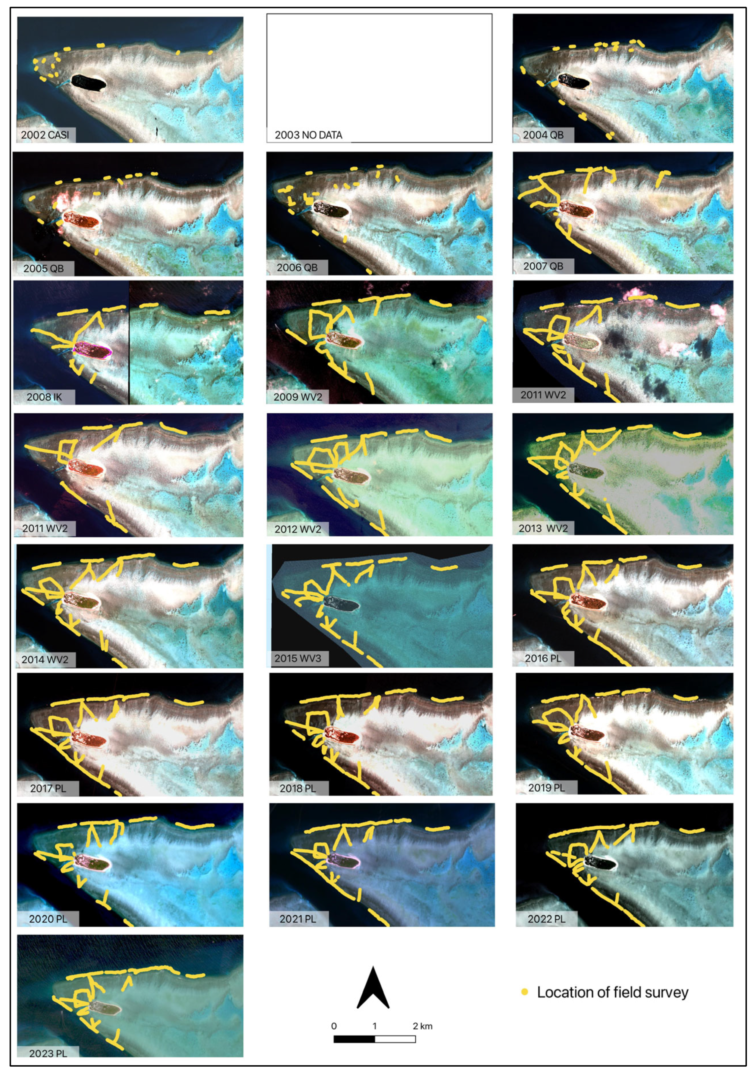
2.2.1. Field Data Collection and Pre-Processing

The benthic composition data were derived from geolocated photoquadrats collected annually over the different geomorphic zones of the reef between 2002 and 2023 (except for 2003); see detailed description in Roelfsema et al., 2021 [36]. In short, 3000–6000 photoquadrats representing a 1 m2 footprint of the bottom were captured every 2–4 m along imaginary transects 500–1500 m in length. A GPS was used to track the survey position in a float towed by a diver or snorkeler, and photoquadrats could be geolocated using time synchronization. Photoquadrats were collected for the reef flat (0.5–2 m depth) by a snorkeler and for the reef slope (4–7 m depth) by a scuba diver.
Benthic composition and abundance were derived from each photoquadrat through two machine learning packages: CoralNet [48] for the years 2002 to 2018 and ReefCloud [49] for 2019 to 2023. The CoralNet model (2002–2018) had an overall accuracy of 79% [36], and the ReefCloud model (2019–2023) had an overall accuracy of 83%. The 34 subcategories were merged to form four aggregated major representative benthic classes: Coral, Algae, Rock, and Sand (Table A1). The mapping classes were not divided further (i.e., by coral morphology or species) because coral mapping methodologies using multi-spectral satellite imagery, like that of this study, have not shown the ability to classify coral communities in further thematic detail. However, these major benthic classes (Coral, Algae, Rock, and Sand) are the most relevant categories for management and research purposes and have been previously distinguished via remote sensing techniques [43]. Photoquadrats in which the total sum of the four mapping categories (Coral, Algae, Rock, and Sand) was less than 90% were removed. This helped to filter out photos that were either too blurry or of inadequate quality for the annotation software to classify.
We assigned each photoquadrat to one of six dominant benthic mapping classes: Coral, Rock, Rock/Coral, Sand, Sand/Coral, and Mixed. Classification thresholds were based on the Australian Institute of Marine Science (AIMS) Annual Summary Report of Coral Reef Condition [50]. Coral-containing mapping classes were established using the following thresholds: “Coral” = >30% Coral; “Rock/Coral” = Rock > 50% and Coral = 5–30%; and “Sand/Coral” = Sand > 50% and Coral = 5–30%. The remaining mapping classes were established with the following thresholds: “Rock” = >50% Rock; “Sand” = >50% Sand. Photoquadrats that could not be assigned to these mapping classes were considered as the “Mixed” class.

2.2.2. Satellite Imagery Collection and Pre-Processing

High-spatial-resolution (1–4 m) multi-spectral imagery was captured as close as possible to the field data collection dates. For 2002–2015, the sensors were specially programmed to acquire imagery over the study site. The image sensors included the following: Compact Airborne Spectrographic Imager (CASI—Itres Research Ltd., Calgary, AL, Canada), QuickBird-2 (Ball Aerospace & Technologies Corp., Broomfield, CO, USA), IKONOS (Lockheed Martin Space Systems, Littleton, CO, USA), WorldView-2 (Ball Aerospace & Technologies Corp, Broomfield, CO, USA), WorldView-3 (Call Aerospace & Technologies Corp, Broomfield, CO, USA), and Planet Dove (Planet Labs, San Francisco, CA, USA) (Table A2). Atmospheric correction to surface reflectance of the images from 2002–2015 was conducted with the FLAASH® (Fast Line-of-sight Atmospheric Analysis) module in ENVI®4.8 for surface reflectance [51]. For the remaining period, 2016–2023, cloud-free Planet Dove atmospherically corrected at-surface-reflectance imagery was selected closest to the date of field data collection from the Planet Explorer platform [52]. The satellite imagery from 2000 to 2015 were all co-registered by using a differential GPS and using the clearest image as a reference image (2006). The imagery from 2016 to 2023 originated from the same provider (Planet Labs), which bypassed the need to co-register the images.
The at-surface-reflectance imagery was imported into the cloud-based open-access platform Google Earth Engine (GEE) for further processing. We calculated statistical bands for each image to add a more robust set of parameters to be used later in the classification algorithm. These included the following: mean, median, standard deviation, and texture measurements from the gray-level co-occurrence matrix (GLCM), principal component analysis (PCA), and simple non-iterative clustering (SNIC) segmentation [53,54,55,56,57].

2.2.3. Physical Attributes

Three static physical attributes (i.e., they did not change throughout the time-series analysis) that help to characterize coral reef habitats were derived from previous research: depth, slope, and waves [58,59]. Previous research has shown that the inclusion of these layers helps to improve coral mapping products via remote sensing [60,61]. Depth was calculated to 10 m mean sea level (MSL) using bathymetry models derived from Sentinel-2 satellite imagery, and subsequently, depth was used to calculate slope angles [58]. Wave parameters were calculated using wind data and modeled wave exposure [59].

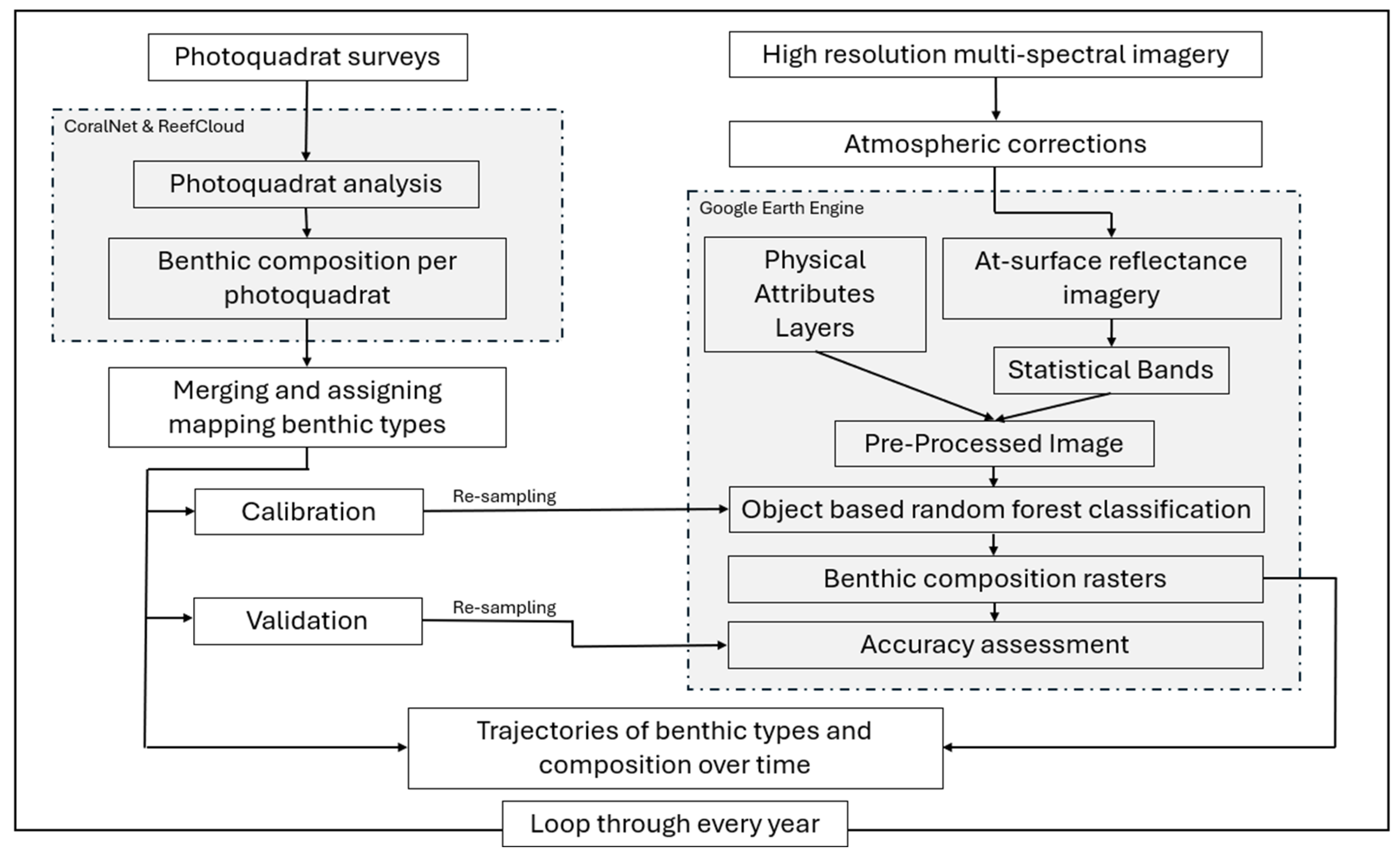
2.3. Habitat Mapping and Accuracy Assessment

Benthic habitat maps were generated through a series of scripts in GEE that included creating calibration and validation sets from the field data, benthic map class assignment, and an accuracy assessment based on approaches developed previously [56,62].
Calibration and validation datasets were created by splitting the field dataset 4:1, respectively. To ensure representation across all the classes for each year analyzed, both the calibration and validation points were re-sampled based on the original field data using the ‘.randomPoints’ built-in function of GEE [56].
For the yearly benthic habitat classification, the calibration points were overlayed with the corresponding processed image and co-variables associated with each benthic type. The co-variables for each calibration point were used to automatically train an RF classifier followed by an object-based automated contextual editing approach [56,62]. This process was repeated for each year, resulting in 21 habitat maps in which each pixel was assigned one of the following mapping classes: Coral, Rock, Rock/Coral, Sand, Sand/Coral, and Mixed. Hereafter, the cover of the mapping class “Coral” (where coral cover = >30%) is used to quantify “coral cover” in the resulting classified rasters and subsequent analysis.
For the accuracy assessment, the field data not used for the classification were used for the validation and compared with the mapped classes each year through an error matrix. Accuracy measures were derived from the error matrix and included overall, producer, and user accuracies [63].

2.4. Trend Analyses

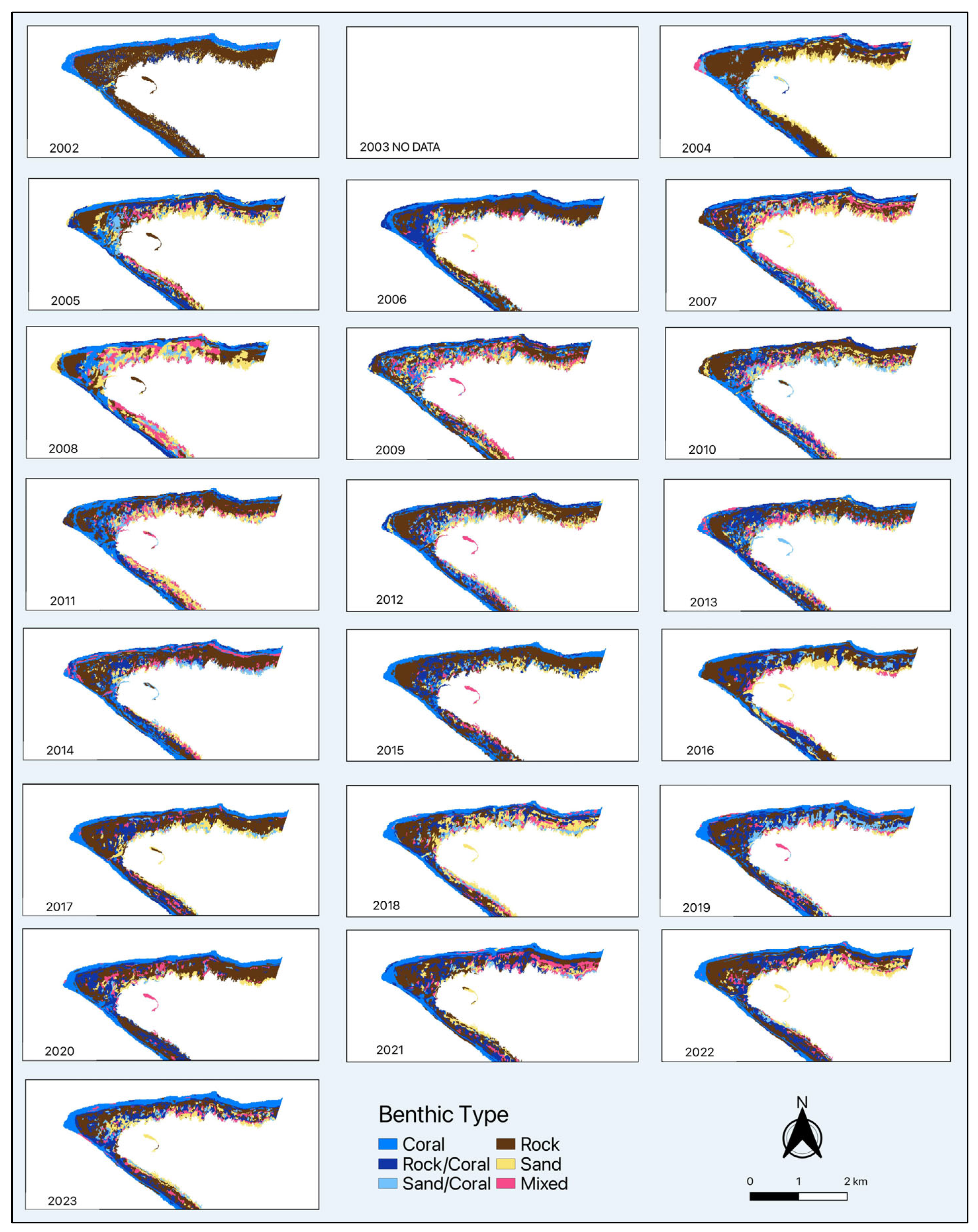
2.4.1. Analyses of Surface Area and Trajectories of the Benthic Cover Types

Annual satellite-derived surface area per benthic mapping class was extracted by vectorizing each classification raster and computing the total surface area of each class in square kilometers.
To compare the resulting classification of the satellite imagery to the field data, percent cover per benthic type per year was calculated for both the field datasets and remote-sensing-derived benthic classification at the geomorphic zone scale (i.e., outer reef flat and reef slope).
For the field datasets, the percent cover per benthic type was calculated based on the number of photoquadrats per benthic mapping class. For the remote-sensing-derived benthic classification rasters, the total surface area of each benthic mapping class was used to calculate percent cover per type using the total surface area of the study area.

2.4.2. Analyses of Coral Cover Trajectories and Temporal Resolution

To analyze the temporal trends in percent coral cover, we applied General Additive Models (GAMs), which compared the field data and the resulting satellite-derived classifications. This analysis was applied to the coral data of the reef slope, given the high coral cover of this portion of the reef. The GAMs used proportional cover as a response variable and the sample year as the predictor variable and were fit as a thin-plate spline. We fit the model using a beta distribution (with logit link function). The GAMs were selected for their ability to model non-linear relationships, allowing us to capture the complex dynamics of coral cover and their changes throughout time. We fit one GAM run for the coral cover vs. sample year for all the satellite data and another GAM run for the coral cover vs. sample year for the field data. The predictions from each model run were drawn and compared to each other to assess the agreement between the two datasets.
Additionally, to evaluate the consistency of model predictions and explore how varying temporal resolutions impact trend identification, we applied GAMs to data subsets representing different time intervals (2 years, 3 years, 4 years, and 5 years). To account for the influence of starting points in our temporal resolution analysis, we included multiple offset variations for each interval (e.g., 3-year intervals starting in 2002, 2004, and 2005) in the GAMs. This ensured that our results captured the full range of possible temporal alignments. This approach allowed us to assess the robustness of remote sensing findings across different temporal scales by detecting changes due to disturbance or recovery and ensuring a comprehensive understanding of and the reliability of the observed trajectories.

3. Results

3.1. Habitat Mapping and Accuracy Assessment

A total of 21 benthic habitat maps were created for the western portion of Heron Reef that included the outer reef flat and reef slope (Figure 4). Visually, the consistent presence of the Coral class in the reef slope and the dominance of the Rock class in the outer reef flat were evident, while the Sand class appeared to be mostly assigned to the outer reef flat areas neighboring the inner reef flat (Figure 4).
The overall accuracy of the time-series maps was 67% and ranged from 59 to 81% (Table 1). The 2002 classification resulted in the highest accuracy, and the 2008 classification had the lowest overall accuracy. The producer accuracies were between 38% and 88%, with the lowest accuracy being for the Rock/Coral class and the highest for the Sand/Coral class. The average user accuracy was between 62% and 69%, with the lowest being from the Rock/Coral class and the highest from the Sand class (Table 1). The number of resulting calibration and validation points vary every year due to the resampling of the number of initial field data points per year; years with more initial field data points had higher numbers of calibration and validation points (Table 1).

3.2. Trend Analyses

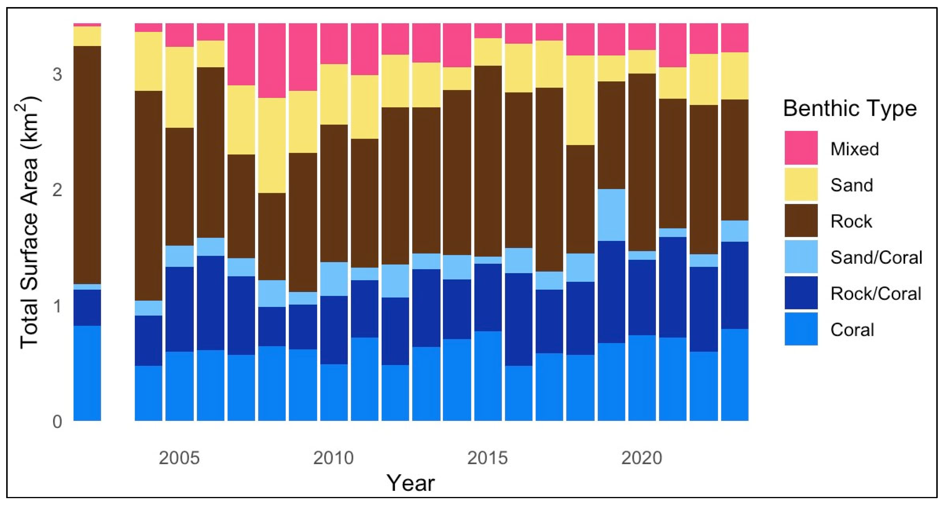
3.2.1. Trends in Surface Area

The surface area for each benthic type was calculated for the western part (3.44 km2) of Heron Reef from 2002 to 2023. The resulting trends showed notable patterns of stability and variation among the different classes (Figure 5). The Coral class maintained a relatively consistent surface area with an average of 0.63 km2 (18.3%) throughout the entire period. The Rock class represented the largest cover of all the benthic types with an average of 1.29 km2 (37.5%) and exhibited moderate fluctuations over time, with peaks in the years when the coral cover was lower (2004, 2010, 2012, and 2016). The Rock/Coral class showed more variability, particularly from 2005 to 2012, with an average of 0.62 km2 (18.0%). The Sand and Mixed classes displayed a smaller, but relatively steady coverage with an average of 0.43 km2 (12.5%) and 0.29 km2 (8.4%), respectively. The Sand/Coral class, though consistently present, maintained the smallest proportion of the total surface area throughout the time series with an average of 0.17 km2 (4.9%).

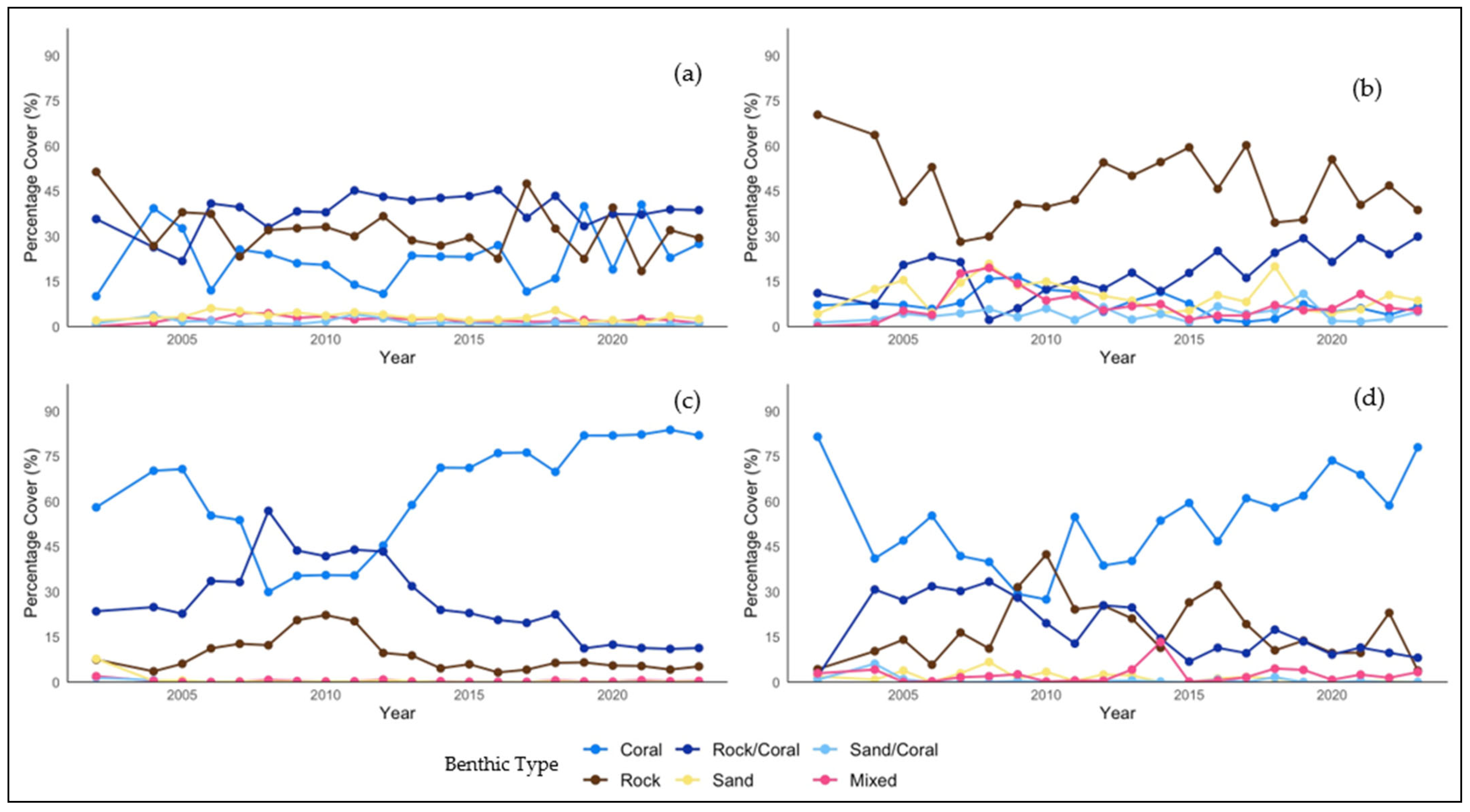
3.2.2. Trends of Percent Cover for Field and Satellite Data

The analysis of benthic cover for Western Heron Reef highlights key differences and similarities between the field data and satellite-derived classifications over the time series from 2002 to 2023 (Figure 6). For the outer reef flat, the field data revealed no clear dominant class, though the Rock/Coral class consistently maintained a slightly higher percent cover than the others, particularly after 2006, with values ranging from 30 to 40% (Figure 6a). The Rock class followed closely, staying between 25 and 40% after 2004 and peaking at 47% in 2017. The Coral class showed lower and more variable cover, dropping to 11% and 16% in 2012 and 2018, respectively, but generally fluctuating from 20 to 40% between 2007 and 2023. The Sand, Sand/Coral, and Mixed classes remained as minor components of the benthic composition with between 0.3 and 10% cover.
The satellite classification for the outer reef flat identified the Rock class as dominant, starting at 70% in 2002 and stabilizing between ~35 and 55% in subsequent years, with a notable drop to ~28% in 2007 (Figure 6b). The Rock/Coral class peaked early at 23% in 2006 but dropped significantly to 2% by 2008 and then gradually increased to 30% by 2023. The Coral class exhibited a lower range of ~1–15%, while the Sand and Mixed classes were consistently between ~5 and 20%. The Sand/Coral class remained the least represented, typically within 1–6%, except for the peak at 10% in 2019.
In contrast to the outer reef flat, the reef slope showed a distinct dominance of the Coral class in both the field and satellite data (Figure 6c,d). The field data indicated an increase in coral cover from 58% in 2002 to a peak of 70% in 2005, followed by a decline to 30% in 2008, and a recovery to 76% in 2016, stabilizing at 70–80% in the following years and then reaching 82% in 2023 (Figure 6c). The Rock and Rock/Coral classes showed inverse trends to that of the Coral class, initially rising to peaks of 22% and 57% by 2010 and 2008, respectively, before declining to 11% and 6% by 2023. Minor classes like the Sand, Sand/Coral, and Mixed classes had minimal presence, each staying within 0.1 and 0.6% after 2004.
The satellite data for the reef slope aligned more closely with the field observations, confirming the Coral class was dominant (Figure 6d). The coral cover was high at 81% in 2002, decreased to 27% by 2010, and then experienced an upward trend, reaching 78% in 2023. The Rock class began at 4% in 2002, peaked at 42% in 2010, and dropped to 11% by 2014, with fluctuations leading to a final cover of 9% in 2023. The Rock/Coral class followed a similar fluctuating pattern, peaking at 30% in the mid-2000s and then gradually decreasing to 8% by 2023. The Sand, Sand/Coral, and Mixed classes remained low, mostly within 0 and 5%, except for a 10% peak for the Mixed class in 2014.

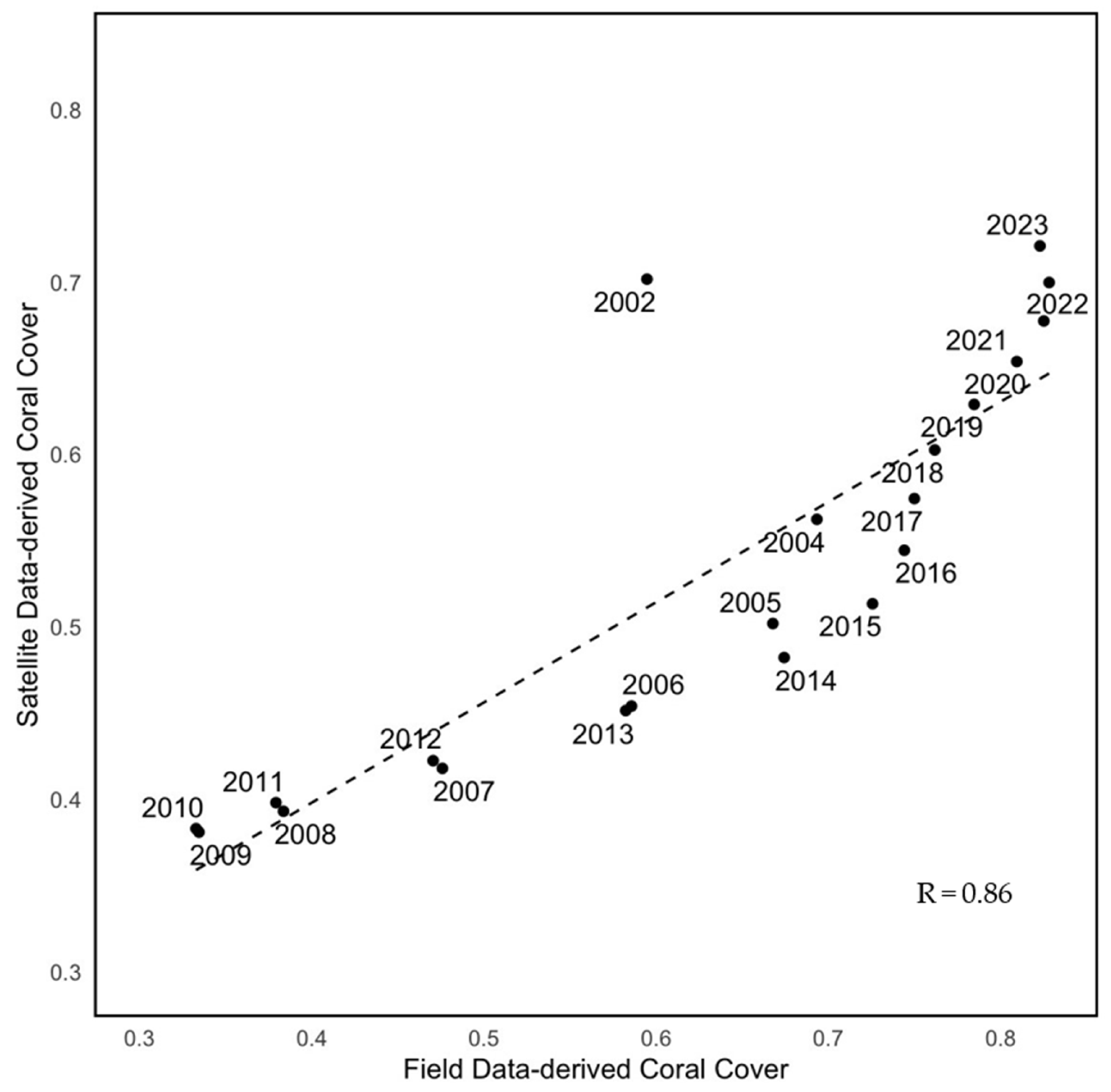
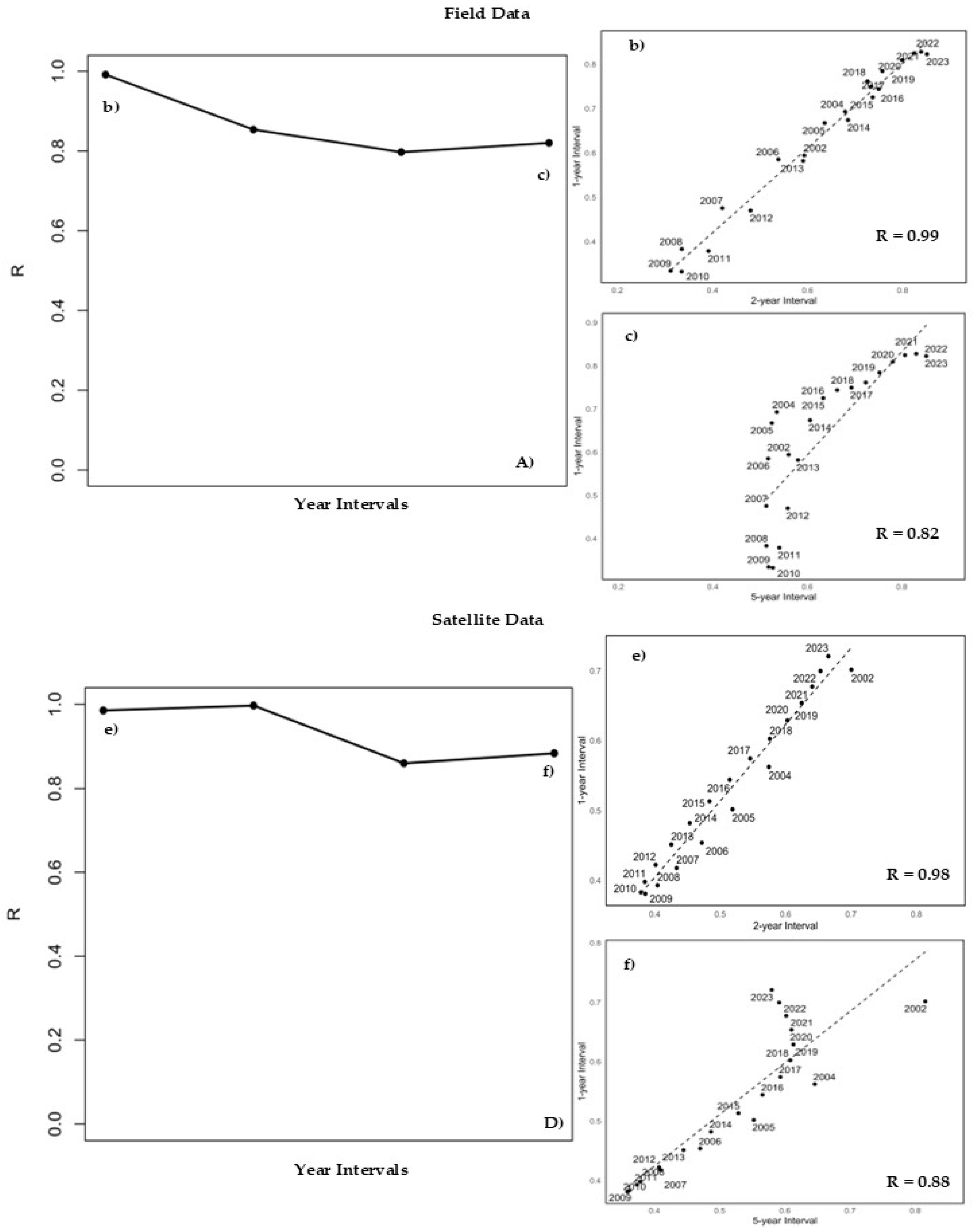
3.2.3. Trends of Coral Cover and Temporal Resolution Analysis

The satellite-derived coral trajectories align closely with the field observations indicated by the resulting GAM analysis between the field and satellite data as a response of the predictor variable (sample year), as it showed a strong positive correlation (R = 0.86) between the two data sources (Figure 7). The high degree of correlation supports the use of satellite imagery as a reliable methodology to identify and quantify changes in the benthic composition of a coral reef through time.
The field and satellite data showed similar results regarding the influence of the temporal resolution on coral trend identification, i.e., the changes in coral cover over time (Figure 8A,D). Both datasets exhibited a strong correlation at the 2-year time interval (R = 0.99), demonstrating that monitoring at 2-year intervals resulted in a minimal loss of trend accuracy (Figure 8b,e). Similar results were also apparent at the 3-year interval (R = 0.85 for the field data and R = 0.99 for the satellite data—Figure 8A,D). When limiting the temporal resolution to 4- and 5-year intervals, the correlation of the coral trajectories decreased considerably (Figure 8A,c,D,f).
Additionally, our results indicated that the choice of starting year had little influence, as variations in interval offsets produced highly similar correlations (Table A3). The 2- and 3-year intervals showed consistent patterns in terms of their trends, whereas the 4- and 5-year intervals exhibited high variability, suggesting that shorter intervals provide a more reliable temporal resolution for mapping. Both the field and satellite datasets showed consistent patterns across the intervals, reinforcing the notion that benthic changes identified by satellite imagery are reliable and consistent with those identified by field techniques.

4. Discussion

4.1. Overall Findings

Here, we demonstrated the ability to create satellite-derived annual benthic habitat maps for the period 2002–2023, enabling the monitoring of trends in benthic habitat types. We developed and implemented a repeatable and accurate mapping approach that integrated in situ field data and high-resolution satellite imagery with machine learning and contextual editing. Remote sensing techniques allowed for the determination of surface area metrics from benthic mapping, providing a broader spatial perspective of benthic changes [64] than field-based data points can provide [65]. This ability to calculate surface area information creates a more nuanced view of the reef’s response to multiple stressful events through time [66]. Remote sensing expands both spatial and temporal coverage and increases repeatability and consistency, representing an overall positive balance for monitoring efforts [67].
Our findings highlighted the importance of determining the appropriate frequency when monitoring reefs using remote sensing, particularly considering the dynamics of disturbance and recovery [68,69]. We found that monitoring every 2 to 3 years provided similar and ecologically relevant insights into the benthic composition over time. Longer intervals of time (i.e., 4- and 5-year intervals) risk smoothing over critical ecological changes, such as periods of decline and recovery. Our observations align with field-based research that has demonstrated slow coral growth and reef accretion rates of just a few millimeters a year [70,71] and contrasting rapid shifts in high coral cover to, for example, macroalgae-dominated systems [72]. Therefore, monitoring coral reefs via remote sensing every 2 to 3 years not only helps to optimize resources but also ensures that critical ecological transitions (i.e., ecological trajectories) are effectively captured, providing a more comprehensive understanding of cycles of reef disturbance and recovery. However, a 2–3-year sampling regime may be most applicable to “healthier” reefs such as Heron Reef, where fast-growing coral communities can rapidly recover from disturbance events. In contrast, reefs that experience more frequent and severe disturbance events should be monitored at shorter intervals (i.e., annually or more frequently depending on the occurrence of disturbances).
The accuracy levels of the remote sensing products described here are comparable with those of mapping efforts for more homogeneous ecosystems (e.g., seagrass meadows), regardless of imagery resolution [73] or other coral reef habitat mapping efforts [74,75]. Classification accuracy appears to be linked to image resolution; CASI (with a 1 m resolution) had the highest overall accuracy (2002, 81%) and Ikonos (with a 4 m resolution) had the lowest (2008, 59%). The classifications of imagery with similar resolutions, i.e., 2004–2007 = 2.4 m (QB), 2009–2015 = 2 m (WV2/3), and 2016–2023 = 3 m (Pl), showed comparable accuracy averages of 66%, 68%, and 67% respectively. However, before 2016, image collection required the sensor be pre-programmed, resulting in environmental conditions that could be unknown or unfavorable for appropriate image quality. After 2016, due to the Planet Dove constellation which guarantees almost daily image capture, optimal imagery could be chosen from an archive or could occur during field surveys [52]. As a result, an image can be previewed for the area of interest and selected considering the date and time of collection and environmental factors, such as cloud cover and tidal stage.

4.2. Ecological Relevance

Our results offer insights into the dynamics of reef health at Heron Reef. This is particularly crucial when understanding how different portions of the reef react differently to stressors [76,77], which can be influenced by environmental factors such as depth, hydrodynamics, and temperature [78,79]. This analysis can also help to identify appropriate ecological baselines, which are crucial for interpreting changes in the reef composition and reef response to disturbances [80].
Overall, the resulting maps showed recovery in coral cover from 2008 to 2023, which aligns with previous field-based research in other reef systems throughout the GBR [81,82] and with previous analyses of the Heron field data [44,47]. This is highly driven by the dominance of fast-growing Acropora species in Heron Reef [81]. Additionally, the satellite-based trajectories also displayed the different disturbance events that Heron faced in the last two decades. Disturbance events included outbreaks of coral diseases (2004–2008) [83,84], an extreme weather event (2015) [44], and coral bleaching events in 2016 and 2017 [85]. While the bleaching events were minor in Heron and in the Southern GBR due to cooler waters compared to the Northern GBR [85,86], the other disturbances (i.e., disease outbreaks and severe weather) are evident in the trajectories of the different benthic mapping classes, particularly in the reef slope.
The analysis of benthic types in different geomorphic zones showed that the trajectories and trends in a reef can differ at within-reef-scales, which might be explained by different factors such as community composition (i.e., different morphologies and species) as well as environmental characteristics such as hydrodynamics and temperature [87,88]. This ability to reliably identify trends via remote sensing techniques might play an even more valuable role in areas in which resources are more limited for field surveys, for reefs that are too remote to access, or in cases in which accessibility between and within reefs is challenging for monitoring finer-scale ecological processes.
While changes in coral cover remains one of the most common indicators of reef health, it is also relevant to consider that the resulting maps and trajectories represent a 2D distribution of benthic cover. However, coral reefs are characterized by their 3D complexity, usually driven by the vertical and horizontal growth of species, which is a key characteristic of their ecosystem processes and services and associated high levels of biodiversity [89]. Even though recent research has shown the ability to calculate 3D complexity via remote sensing at the geomorphic zone scale [58], further research is needed to extract or empirically determine complexity at finer scales, such as morphology types. By integrating the up-scaling capability of remote sensing with the ecological knowledge provided by field data (e.g., coral morphology types), the combination of both methodologies can be useful to better quantify a reef’s ecosystem services and ecological processes [90]. These considerations represent a trade-off, in which field data allow for more in-depth and higher thematic level analyses but are limited to point data, while remote sensing provides wider spatial ranges that can identify changes in the benthic composition beyond single points.

4.3. Limitations and Potential Solutions

The characteristic heterogeneity of coral reefs represents one of the major challenges for mapping benthic composition in these habitats [25]. For coral reefs, one pixel may contain several benthic types, and the percent cover of each may change from pixel to pixel depending on the sensor resolution [91], which does not occur in more spectrally homogeneous habitats such as land ecosystems [92] and seagrass beds [73]. Additionally, the field data consisted of photoquadrats of roughly 1 × 1 m, while the pixels in the images for this study had different resolutions (2 × 2 m, 2.4 × 2.4 m, and 3 × 3 m). This impacts classifier training, as the spectral signatures of the benthic types in the photoquadrats may represent a small fraction of the area covered by the corresponding satellite pixel (e.g., 11% of a 3 × 3 m pixel) [46]. In addition, the location of the transects in different geomorphic zones might have potentially altered the levels of accuracy and the trends in composition, given the different characteristics of each zone of the reef, especially between reef slope and reef flat zones. For instance, while Heron Reef’s slope is more spectrally homogenous due to the high coral cover, the outer reef flat is a more spectrally fragmented habitat. A potential solution is to establish mapping benthic types specific to the ecosystem, obtaining the percent cover of each benthic type, and understanding how they are classified (i.e., mixed classes) [93].
While the heterogeneity of the habitat makes it difficult to accurately map each benthic class, the intrinsic spectral characteristics of the benthic types also make it difficult to differentiate the classes from one another. Although high-resolution imagery has been shown to distinguish between coral and algae within reef habitats, these benthic types still exhibit very similar spectral characteristics [94,95]. In this study, the “Rock” class includes rubble and dead hard coral overgrown with crustose coralline algae or algal mats, both of which present spectral features typical of algae [96,97]. Consequently, the spectral signatures of the “Coral”, “Rock”, and “Rock/Coral” classes overlap considerably, which may reduce the classification accuracy for these categories. A clear example is the average accuracies of the “Rock/Coral” class, which are the lowest among all average accuracies per class across the years (average producer accuracy = 38% and average user accuracy = 62%; Table 1). A potential way to address this challenge is to find ways to standardize different thresholds of the percent cover per class, e.g., Sand/Coral vs. Rock/Coral, based on levels of heterogeneity, spectral mixing, or ecologically relevant coral cover thresholds.
Light attenuation driven by the reduced intensity of light penetration through the water column might have an influence in the mapping products. This may also vary across geomorphic zones. While light attenuation may be more evident in the reef slope (2–10 m depth), it can also play a role in the reef flat (~2 m depth). This may be relevant in the mapping accuracy as it might reduce light reflectance by the different benthic types [97,98,99]. While we aimed to mitigate this by including physical attribute layers (depth, slope, and waves), this could potentially be further refined by evaluating the influence of water column corrections to the images on the resulting mapping accuracies.
Mapping errors can be introduced by field data collection and processing, affecting accuracy levels. The labeling of each photoquadrat is automated, and an error in the annotation software may result in the misclassification of the photoquadrats. This error may be due to photoquadrat quality, light intensity, human annotation training, the complexity of the label set, camera settings/quality, and the distance from the camera to the substrate [48,93]. Consistency in the annotation methods is crucial to minimize these errors.
The hand-held GPS receiver used for the field work generally has an accuracy of 5–10 m, which can affect the assigned geolocation of the photoquadrat. The level of influence of these errors can be amplified by georeferencing errors from the satellite imagery and depend on the abiotic factors (depth, habitat complexity, slope, currents, and wind) of the area where each data point is collected [100]. Even though these situations are difficult to control and may vary depending on reef characteristics and weather conditions, the detailed planning of field data collection campaigns can potentially minimize these errors.

4.4. Future Research

Understanding the distribution and trajectories of coral morphologies is of importance for assessing reef restoration and conservation efforts [101]. Future works should concentrate on identifying finer thematic and spatial scale changes by examining variations at different levels, such as coral morphologies, and by using higher-resolution remote sensing imagery [102]. Additionally, understanding the spatial proximity between different benthic cover types would provide insights into the complexity of coral reefs.
This study focused on the western part of Heron Reef, with copious detailed field data. Future research should focus on mapping the whole reef and establishing the optimal amount and spatial distribution of field data required for accurately and reliably mapping the benthic composition at the entire-reef scale through space and time [103].
Given the increase in mass bleaching events, assessing how this method can detect coral bleaching and its impact on benthic composition should be a priority in future works [104,105,106]. Heron Reef was impacted by the 2024 mass bleaching event; however, an assessment of its impact falls out of the scope of this current study.
The mapping approach could be repeated for other reef areas once high-resolution imagery, coincident field data, and physical attributes (depth, slope, and waves) are available. However, to evaluate its effectiveness, it is important to conduct a sensitivity analysis to determine the extent of change in the benthic cover required for accurate detection using the approach presented here.

5. Conclusions

This study demonstrated the capability to produce accurate coral reef habitat maps annually using a robust and repeatable remote sensing-based approach and to generate spatially explicit information regarding coral reef trends over a long time series. By combining in situ data with high-spatial-resolution multi-spectral satellite imagery and RF-based classifications, we demonstrated that the methodology presented can effectively capture spatial and temporal changes in benthic types at the reef and within-reef scales. The information derived from this time-series analysis provided surface area metrics and detected ecological trajectories, such as those of coral disturbance and recovery. Additionally, our results also highlighted the spatial trade-off for coral reef managers when using either our methodology or traditional field monitoring. Our methodology allows for monitoring larger areas of the reef but with a limited level of thematic detail.
Our findings suggest that remote-sensing-based monitoring at 2- and 3-year intervals might provide a balance between resource efficiency and ecological relevance, capturing critical changes in benthic composition, while assuming minimal additional disturbances/impacts. Despite challenges such as habitat heterogeneity and classification errors, this approach offered a scalable and repeatable methodology. When paired with detailed insights from field-based monitoring, remote sensing enhances our capacity to understand and manage coral reef ecosystems. This integrative framework provides a standardized approach for monitoring reef health, with implications for conservation and management strategies applicable to other reef systems.

Author Contributions

Conceptualization, D.E.C.R., E.K. and C.M.R.; methodology, D.E.C.R., F.F.D., N.M.H., T.S., E.K., K.M. and C.M.R.; software, D.E.C.R. and C.M.R.; validation, D.E.C.R. and T.S.; formal analysis, D.E.C.R., F.F.D., N.M.H., T.S. and C.M.R.; resources, C.M.R.; data curation, D.E.C.R., F.F.D., E.K., K.M. and C.M.R.; writing—original draft preparation, D.E.C.R., F.F.D., N.M.H. and C.M.R.; writing—review and editing, D.E.C.R., F.F.D., N.M.H., T.S., E.K., K.M. and C.M.R.; visualization, D.E.C.R., F.F.D., N.M.H., T.S. and C.M.R.; supervision, C.M.R.; project administration, E.K., K.M. and C.M.R.; funding acquisition, C.M.R. All authors have read and agreed to the published version of the manuscript.

Funding

This research was funded by the University of Queensland; Global Change Institute at UQ, CSIRO; the ARC Laureate Fellowship awarded to Professor Ove Hoegh-Guldberg; an ARC Linkage Grant to Prof. J Marshall and Prof. S Phinn; WBGef Coral Reef Remote Sensing; ARC linkage innovative Coral Reef Monitoring; the Allen Coral Atlas; the Lott; the Great Barrier Reef Foundation; and the Great Barrier Marine Park Authority.

Data Availability Statement

Field and satellite data can be accessed upon request. The pre-processing of field data and the habitat mapping scripts can be found via the following link: https://github.com/memlUQ/HRTimeSeries/tree/main.

Acknowledgments

We acknowledge the traditional owners and show our respect to the past, present, and emerging people of Bailai, Gurang, Gooreng Gooreng, and Taribelang of the Heron Reef Sea country, in which we conducted the field work with their consent. We would like to thank Stuart Phinn for his ongoing support in the long-term monitoring of Heron Reef. Fieldwork support was provided by CoralWatch and Reef Check volunteers, staff and students at University of Queensland, and the Heron Island Research Station. Field assistance was provided by Peran Bray, Rodney Borrego, Robert Canto, Stevo Carbonara, Diana Kleine, Ian Leiper, Jennifer Lodder, Mitchell Lyons, Josh Passenger, Meredith Roe, Jodi Samon, Megan Saunders, Joanna Smart, Dylan Cowley, Kirsten Golding, Douglas Stetner, and Jeremy Wolf.

Conflicts of Interest

The funders had no role in the design of the study; in the collection, analyses, or interpretation of data; in the writing of the manuscript; or in the decision to publish the results.

Appendix A

Table A1. Benthic composition within each photoquadrat was determined through machine learning using a label set that included 34 benthic composition classes, which were then grouped into four mapping classes [36].
Mapping ClassesBenthic Composition Classes
CoralAcropora Branching
Acropora Digitate
Acropora Hispidose
Acropora Tabulate and Corymbose
Acroporidae Plate Encrusting (Montipora)
Acropora Other (Isopora)
Porites Branching
Porites Encrusting
Porites Massive
Favid Mussid
Foliose or Plate with ridges
Foliose or Plate with round coralites
Gorgonian
Pocillopora
Branching Other
Massive Other
Hard Coral Other
Alcyoniidae Soft Coral
Soft Coral Other
AlgaeAlgae Other
Chlorodesmis species
Caulerpa species
Cyano species
Dictyota species
Halimeda species
Lobophora species
Padina species
Turbinaria species
Benthic Micro Algae on Sand
Algae Other
RockCrustose Coraline Algae on:
  • dead hard coral
  • rubble
Epithelial Algal Matrix on:
  • dead hard coral
  • rubble
SandSand
Table A2. Characteristics of the field data and high-resolution multi-spectral satellite imagery used. CASI = Compact Airborne Spectrographic Imager; QB = QuickBird; IK = Ikonos; WV2 = WorldView-2; WV3 = WorldView-3; PL = Planet; H > L = high to low tide; L > H = low to high tide; FLAASH = Fast Line-of-sight Atmospheric Analysis; Unk. = Unknown.
YearField Data Points (#)SensorResolution (m)Atmospheric CorrectionField Data
Collection
(dd–dd/mm)
Image
Acquisition
(dd/mm)
Difference
Field/Image
Acquisition (days)
Tide at Image
Acquisition
2002561CASI1FLAASH®25–28/0602/074High
20041425QB2.4FLAASH®20–22/0517/053Mid (H > L)
2005705QB2.4FLAASH®21–24/0625/061Mid (H > L)
20061035QB2.4FLAASH®25/06–01/0703/0834Low
20071830QB2.4FLAASH®23–27/0907/0757High
20081698IK4FLAASH®25–30/1017/0938High
20092955WV22FLAASH®2–6/1115/1239High
20103210WV22FLAASH®10–12/1122/05/11137Mid (L > H)
20112111WV22FLAASH®1–4/1130/102Mid (L > H)
20122775WV22FLAASH®1–5/0729/0855Mid (H > L)
20132635WV22FLAASH®2–6/1112/116Mid (H > L)
20142713WV22FLAASH®7–13/1101/1037Mid (L > H)
20152411WV32FLAASH®24–28/1114/1110High
20162397PL3Planet Labs17–22/0926/094Mid (L > H)
20173803PL3Planet Labs29/10–3/1105/1024High
20182805PL3Planet Labs11–16/1106/115High
20194085PL3Planet Labs28–31/1008/118Mid (H > L)
20204506PL3Planet Labs31/10–5/1105/110Mid (L > H)
20214852PL3Planet Labs6–11/1127/1010Mid (L > H)
20225483PL3Planet Labs4–12/1101/113Mid (L > H)
20236238PL3Planet Labs27/10–2/1110/118Mid (H > L)
Table A3. R values for the field and satellite data across the different temporal intervals (2-, 3-, 4-, and 5-year intervals) at each starting year offset.
R Value for Each Starting Year Offset
Satellite Imagery Year Intervals20022004200520062007
2-year0.990.99
3-year0.990.870.99
4-year0.860.810.980.86
5-year0.880.550.760.840.88
R Value for Each Starting Year Offset
Field Data Year Intervals20022004200520062007
2-year0.990.99
3-year0.850.930.85
4-year0.800.920.920.80
5-year0.820.920.920.630.82

References

  1. Hughes, T.P.; Baird, A.H.; Bellwood, D.R.; Card, M.; Connolly, S.R.; Folke, C.; Grosberg, R.; Hoegh-Guldberg, O.; Jackson, J.B.C.; Kleypas, J.; et al. Climate change, human impacts, and the resilience of coral reefs. Science 2003, 301, 929–933. [Google Scholar] [CrossRef]
  2. Lapointe, B.E.; Brewton, R.A.; Herren, L.W.; Porter, J.W.; Hu, C.M. Nitrogen enrichment, altered stoichiometry, and coral reef decline at Looe Key, Florida Keys, USA: A 3-decade study. Mar. Biol. 2019, 166, 108. [Google Scholar] [CrossRef]
  3. Johnson, M.D.; Scott, J.J.; Leray, M.; Lucey, N.; Bravo, L.M.R.; Wied, W.L.; Altieri, A.H. Rapid ecosystem-scale consequences of acute deoxygenation on a Caribbean coral reef. Nat. Commun. 2021, 12, 4522. [Google Scholar] [CrossRef]
  4. Zhao, H.W.; Yuan, M.L.; Strokal, M.; Wu, H.C.; Liu, X.H.; Murk, A.; Kroeze, C.; Osinga, R. Impacts of nitrogen pollution on corals in the context of global climate change and potential strategies to conserve coral reefs. Sci. Total Environ. 2021, 774, 145017. [Google Scholar] [CrossRef]
  5. Dornelas, M.; Madin, J.S.; Baird, A.H.; Connolly, S.R. Allometric growth in reef-building corals. Proc. Roy. Soc. B-Biol. Sci. 2017, 284, 20170053. [Google Scholar] [CrossRef]
  6. Glynn, P.W.; Manzello, D.P. Bioerosion and Coral Reef Growth: A Dynamic Balance. In Coral Reefs in the Anthropocene; Springer: Dordrecht, The Netherlands, 2015; pp. 67–97. [Google Scholar] [CrossRef]
  7. Mollica, N.R.; Guo, W.F.; Cohen, A.L.; Huang, K.F.; Foster, G.L.; Donald, H.K.; Solow, A.R. Ocean acidification affects coral growth by reducing skeletal density. Proc. Natl. Acad. Sci. USA 2018, 115, 1754–1759. [Google Scholar] [CrossRef]
  8. Madin, J.S.; Madin, E.M.P. The full extent of the global coral reef crisis. Conserv. Biol. 2015, 29, 1724–1726. [Google Scholar] [CrossRef]
  9. Edmunds, P.J.; Bruno, J.F. The importance of sampling scale in ecology: Kilometer-wide variation in coral reef communities. Mar. Ecol. Prog. Ser. 1996, 143, 165–171. [Google Scholar] [CrossRef]
  10. Cortés, J.; Oxenford, H.A.; van Tussenbroek, B.I.; Jordán-Dahlgren, E.; Cróquer, A.; Bastidas, C.; Ogden, J.C. The CARICOMP Network of Caribbean Marine Laboratories (1985–2007): History, Key Findings, and Lessons Learned. Front. Mar. Sci. 2019, 5, 519. [Google Scholar] [CrossRef]
  11. Ortiz, J.C.; Gomez-Cabrera, M.D.; Hoegh-Guldberg, O. Effect of colony size and surrounding substrate on corals experiencing a mild bleaching event on Heron Island reef flat (southern Great Barrier Reef, Australia). Coral Reefs 2009, 28, 999–1003. [Google Scholar] [CrossRef]
  12. Brown, K.T.; Bender-Champ, D.; Kubicek, A.; van der Zande, R.; Achlatis, M.; Hoegh-Guldberg, O.; Dove, S.G. The Dynamics of Coral-Algal Interactions in Space and Time on the Southern Great Barrier Reef. Front. Mar. Sci. 2018, 5, 181. [Google Scholar] [CrossRef]
  13. Hughes, T.P.; Kerry, J.T.; Baird, A.H.; Connolly, S.R.; Dietzel, A.; Eakin, C.M.; Heron, S.F.; Hoey, A.S.; Hoogenboom, M.O.; Liu, G.; et al. Global warming transforms coral reef assemblages. Nature 2018, 556, 492–496. [Google Scholar] [CrossRef] [PubMed]
  14. De’ath, G.; Fabricius, K.E.; Sweatman, H.; Puotinen, M. The 27-year decline of coral cover on the Great Barrier Reef and its causes. Proc. Natl. Acad. Sci. USA 2012, 109, 17995–17999. [Google Scholar] [CrossRef] [PubMed]
  15. Viehman, T.S.; Hench, J.L.; Griffin, S.P.; Malhotra, A.; Egan, K.; Halpin, P.N. Understanding differential patterns in coral reef recovery: Chronic hydrodynamic disturbance as a limiting mechanism for coral colonization. Mar. Ecol. Prog. Ser. 2018, 605, 135–150. [Google Scholar] [CrossRef]
  16. Roth, F.; Saalmann, F.; Thomson, T.; Coker, D.J.; Villalobos, R.; Jones, B.H.; Wild, C.; Carvalho, S. Coral reef degradation affects the potential for reef recovery after disturbance. Mar. Environ. Res. 2018, 142, 48–58. [Google Scholar] [CrossRef]
  17. Dullo, W.C. Coral growth and reef growth: A brief review. Facies 2005, 51, 33–48. [Google Scholar] [CrossRef]
  18. Rasser, M.W.; Riegl, B. Holocene coral reef rubble and its binding agents. Coral Reefs 2002, 21, 57–72. [Google Scholar] [CrossRef]
  19. Fabricius, K.E.; Crossman, K.; Jonker, M.; Mongin, M.; Thompson, A. Macroalgal cover on coral reefs: Spatial and environmental predictors, and decadal trends in the Great Barrier Reef. PLoS ONE 2023, 18, e0279699. [Google Scholar] [CrossRef]
  20. Andréfouët, S. Coral reef habitat mapping using remote sensing:: A user vs producer perspective.: Implications for research, management and capacity building. J. Spat. Sci. 2008, 53, 113–129. [Google Scholar] [CrossRef]
  21. Mumby, P.J.; Skirving, W.; Strong, A.E.; Hardy, J.T.; LeDrew, E.F.; Hochberg, E.J.; Stumpf, R.P.; David, L.T. Remote sensing of coral reefs and their physical environment. Mar. Pollut. Bull. 2004, 48, 219–228. [Google Scholar] [CrossRef]
  22. Potapov, P.; Hansen, M.C.; Pickens, A.; Hernandez-Serna, A.; Tyukavina, A.; Turubanova, S.; Zalles, V.; Li, X.Y.; Khan, A.; Stolle, F.; et al. The Global 2000–2020 Land Cover and Land Use Change Dataset Derived from the Landsat Archive: First Results. Front. Remote Sens. 2022, 3, 856903. [Google Scholar] [CrossRef]
  23. Zhang, X.; Zhao, T.T.; Xu, H.; Liu, W.D.; Wang, J.Q.; Chen, X.D.; Liu, L.Y. GLC_FCS30D: The first global 30 m land-cover dynamics monitoring product with a fine classification system for the period from 1985 to 2022 generated using dense-time-series Landsat imagery and the continuous change-detection method. Earth Syst. Sci. Data 2024, 16, 1353–1381. [Google Scholar] [CrossRef]
  24. Palandro, D.; Andréfouët, S.; Dustan, P.; Muller-Karger, F.E. Change detection in coral reef communities using Ikonos satellite sensor imagery and historic aerial photographs. Int. J. Remote Sens. 2003, 24, 873–878. [Google Scholar] [CrossRef]
  25. Andréfouët, S.; Muller-Karger, F.E.; Hochberg, E.J.; Hu, C.M.; Carder, K.L. Change detection in shallow coral reef environments using Landsat 7 ETM+ data. Remote Sens. Environ. 2001, 78, 150–162. [Google Scholar] [CrossRef]
  26. Burns, C.; Bollard, B.; Narayanan, A. Machine-Learning for Mapping and Monitoring Shallow Coral Reef Habitats. Remote Sens. 2022, 14, 2666. [Google Scholar] [CrossRef]
  27. Hedley, J.D.; Roelfsema, C.; Brando, V.; Giardino, C.; Kutser, T.; Phinn, S.; Mumby, P.J.; Barrilero, O.; Laporte, J.; Koetz, B. Coral reef applications of Sentinel-2: Coverage, characteristics, bathymetry and benthic mapping with comparison to Landsat 8. Remote Sens. Environ. 2018, 216, 598–614. [Google Scholar] [CrossRef]
  28. Hochberg, E.J. Remote Sensing of Coral Reef Processes. In Coral Reefs: An Ecosystem in Transition; Springer: Dordrecht, The Netherlands, 2011; pp. 25–35. [Google Scholar] [CrossRef]
  29. Andréfouët, S.; Berkelmans, R.; Odriozola, L.; Done, T.; Oliver, J.; Müller-Karger, F. Choosing the appropriate spatial resolution for monitoring coral bleaching events using remote sensing. Coral Reefs 2002, 21, 147–154. [Google Scholar] [CrossRef]
  30. Hedley, J.D.; Roelfsema, C.M.; Chollett, I.; Harborne, A.R.; Heron, S.F.; Weeks, S.J.; Skirving, W.J.; Strong, A.E.; Eakin, C.M.; Christensen, T.R.L.; et al. Remote Sensing of Coral Reefs for Monitoring and Management: A Review. Remote Sens. 2016, 8, 118. [Google Scholar] [CrossRef]
  31. Kennedy, R.E.; Andréfouët, S.; Cohen, W.B.; Gómez, C.; Griffiths, P.; Hais, M.; Healey, S.P.; Helmer, E.H.; Hostert, P.; Lyons, M.B.; et al. Bringing an ecological view of change to Landsat-based remote sensing. Front. Ecol. Environ. 2014, 12, 339–346. [Google Scholar] [CrossRef]
  32. Haya, L.O.M.Y.; Fujii, M. Mapping the change of coral reefs using remote sensing and in situ measurements: A case study in Pangkajene and Kepulauan Regency, Spermonde Archipelago, Indonesia. J. Oceanogr. 2017, 73, 623–645. [Google Scholar] [CrossRef]
  33. Palandro, D.A.; Andréfouët, S.; Hu, C.; Hallock, P.; Müller-Karger, F.E.; Dustan, P.; Callahan, M.K.; Kranenburg, C.; Beaver, C.R. Quantification of two decades of shallow-water coral reef habitat decline in the Florida Keys National Marine Sanctuary using Landsat data (1984–2002). Remote Sens. Environ. 2008, 112, 3388–3399. [Google Scholar] [CrossRef]
  34. Galzin, R.; Lecchini, D.; Lison de Loma, T.; Moritz, C.; Parravicini, V.; Siu, G. Long term monitoring of coral and fish assemblages (1983–2014) in Tiahura reefs, Moorea, French Polynesia. Cybium 2016, 40, 31–41. [Google Scholar]
  35. House, J.E.; Brambilla, V.; Bidaut, L.M.; Christie, A.P.; Pizarro, O.; Madin, J.S.; Dornelas, M. Moving to 3D: Relationships between coral planar area, surface area and volume. Peerj 2018, 6, e4280. [Google Scholar] [CrossRef]
  36. Roelfsema, C.; Kovacs, E.M.; Markey, K.; Vercelloni, J.; Rodriguez-Ramirez, A.; Lopez-Marcano, S.; Gonzalez-Rivero, M.; Hoegh-Guldberg, O.; Phinn, S.R. Benthic and coral reef community field data for Heron Reef, Southern Great Barrier Reef, Australia, 2002–2018. Sci. Data 2021, 8, 84. [Google Scholar] [CrossRef]
  37. Leiper, I.A.; Siebeck, U.E.; Marshall, N.J.; Phinn, S.R. Coral health monitoring: Linking coral colour and remote sensing techniques. Can. J. Remote Sens. 2009, 35, 276–286. [Google Scholar] [CrossRef]
  38. Joyce, K.E.; Phinn, S.R. Bi-directional reflectance of corals. Int. J. Remote Sens. 2002, 23, 389–394. [Google Scholar] [CrossRef]
  39. Joyce, K.E.; Phinn, S.R.; Roelfsema, C.M.; Neil, D.T.; Dennison, W.C. Combining Landsat ETM plus and Reef Check classifications for mapping coral reefs: A critical assessment from the southern Great Barrier Reef, Australia. Coral Reefs 2004, 23, 21–25. [Google Scholar] [CrossRef]
  40. Hedley, J.; Roelfsema, C.; Phinn, S.R. Efficient radiative transfer model inversion for remote sensing applications. Remote Sens. Environ. 2009, 113, 2527–2532. [Google Scholar] [CrossRef]
  41. Han, J.L.; Shoeiby, M.; Malthus, T.; Botha, E.; Anstee, J.; Anwar, S.; Wei, R.; Armin, M.A.; Li, H.D.; Petersson, L. Underwater Image Restoration via Contrastive Learning and a Real-World Dataset. Remote Sens. 2022, 14, 4297. [Google Scholar] [CrossRef]
  42. Roelfsema, C.M.; Phinn, S.R.; Dennison, W.C. Spatial distribution of benthic microalgae on coral reefs determined by remote sensing. Coral Reefs 2002, 21, 264–274. [Google Scholar] [CrossRef]
  43. Roelfsema, C.; Phinn, S.; Jupiter, S.; Comley, J.; Albert, S. Mapping coral reefs at reef to reef-system scales, 10s-1000s km, using object-based image analysis. Int. J. Remote Sens. 2013, 34, 6367–6388. [Google Scholar] [CrossRef]
  44. Vercelloni, J.; Roelfsema, C.; Kovacs, E.M.; Gonzalez-Rivero, M.; Moores, M.T.; Logan, M.; Mengersen, K. Fine-scale interplay between decline and growth determines the spatial recovery of coral communities within a reef. Ecography 2024, 2024, e06818. [Google Scholar] [CrossRef]
  45. Phinn, S.R.; Roelfsema, C.M.; Mumby, P.J. Multi-scale, object-based image analysis for mapping geomorphic and ecological zones on coral reefs. Int. J. Remote Sens. 2011, 33, 3768–3797. [Google Scholar] [CrossRef]
  46. Roelfsema, C.; Kovacs, E.; Roos, P.; Terzano, D.; Lyons, M.; Phinn, S. Use of a semi-automated object based analysis to map benthic composition, Heron Reef, Southern Great Barrier Reef. Remote Sens. Lett. 2018, 9, 324–333. [Google Scholar] [CrossRef]
  47. Roelfsema, C.; Kovacs, E.M.; Vercelloni, J.; Markey, K.; Rodriguez-Ramirez, A.; Lopez-Marcano, S.; Gonzalez-Rivero, M.; Hoegh-Guldberg, O.; Phinn, S.R. Fine-scale time series surveys reveal new insights into spatio-temporal trends in coral cover (2002–2018), of a coral reef on the Southern Great Barrier Reef. Coral Reefs 2021, 40, 1055–1067. [Google Scholar] [CrossRef]
  48. González-Rivero, M.; Beijbom, O.; Rodriguez-Ramirez, A.; Holtrop, T.; González-Marrero, Y.; Ganase, A.; Roelfsema, C.; Phinn, S.; Hoegh-Guldberg, O. Scaling up Ecological Measurements of Coral Reefs Using Semi-Automated Field Image Collection and Analysis. Remote Sens. 2016, 8, 30. [Google Scholar] [CrossRef]
  49. Australian Institute of Marine Science (AIMS). ReefCloud. Available online: https://apps.aims.gov.au/metadata/view/85a61b8d-a626-4c1f-929f-aa8777e268d3 (accessed on 8 January 2024).
  50. Science, A.I.O.M. Annual Summary Report of Coral Reef Condition 2022/23. Available online: https://www.aims.gov.au/monitoring-great-barrier-reef/gbr-condition-summary-2022-23 (accessed on 15 March 2024).
  51. Roelfsema, C.M.; Lyons, M.; Kovacs, E.M.; Maxwell, P.; Saunders, M.I.; Samper-Villarreal, J.; Phinn, S.R. Multi-temporal mapping of seagrass cover, species and biomass: A semi-automated object based image analysis approach. Remote Sens. Environ. 2014, 150, 172–187. [Google Scholar] [CrossRef]
  52. Labs, P. Planet Surface Reflectance Poduct V2.0. Available online: https://assets.planet.com/marketing/PDF/Planet_Surface_Reflectance_Technical_White_Paper.pdf (accessed on 15 March 2024).
  53. Shihavuddin, A.S.M.; Gracias, N.; Garcia, R.; Gleason, A.C.R.; Gintert, B. Image-Based Coral Reef Classification and Thematic Mapping. Remote Sens. 2013, 5, 1809–1841. [Google Scholar] [CrossRef]
  54. Wahidin, N.; Siregar, V.P.; Nababan, B.; Jaya, I.; Wouthuyzen, S. Object-based image analysis for coral reef benthic habitat mapping with several classification algorithms. Procedia Environ. Sci. 2015, 24, 222–227. [Google Scholar] [CrossRef]
  55. Wicaksono, P. Improving the accuracy of Multispectral-based benthic habitats mapping using image rotations: The application of Principle Component Analysis and Independent Component Analysis. Eur. J. Remote Sens. 2016, 49, 433–463. [Google Scholar] [CrossRef]
  56. Lyons, M.B. Earth Engine Catalog. Available online: https://github.com/mitchest/earthengine-catalog (accessed on 8 January 2024).
  57. Haralick, R.M.; Shanmugam, K.; Dinstein, I. Textural Features for Image Classification. IEEE Trans. Syst. Man Cybern. 1973, Smc3, 610–621. [Google Scholar] [CrossRef]
  58. Roelfsema, C.M.; Lyons, M.B.; Castro-Sanguino, C.; Kovacs, E.M.; Callaghan, D.; Wettle, M.; Markey, K.; Borrego-Acevedo, R.; Tudman, P.; Roe, M.; et al. How Much Shallow Coral Habitat Is There on the Great Barrier Reef? Remote Sens. 2021, 13, 4343. [Google Scholar] [CrossRef]
  59. Callaghan, D. Great Barrier Reef Non-Cyclonic and on-Reef Wave Model Predictions; The University of Queensland: Brisbane, QLD, Australia, 2023. [Google Scholar]
  60. Goodman, J.A.; Lay, M.; Ramirez, L.; Ustin, S.L.; Haverkamp, P.J. Confidence Levels, Sensitivity, and the Role of Bathymetry in Coral Reef Remote Sensing. Remote Sens. 2020, 12, 496. [Google Scholar] [CrossRef]
  61. Kennedy, E.V.; Roelfsema, C.M.; Lyons, M.B.; Kovacs, E.M.; Borrego-Acevedo, R.; Roe, M.; Phinn, S.R.; Larsen, K.; Murray, N.J.; Yuwono, D.; et al. Reef Cover, a coral reef classification for global habitat mapping from remote sensing. Sci. Data 2021, 8, 196. [Google Scholar] [CrossRef]
  62. Lyons, M.B.; Roelfsema, C.M.; Kennedy, E.; Kovacs, E.M.; Borrego-Acevedo, R.; Markey, K.; Roe, M.; Yuwono, D.M.; Harris, D.L.; Phinn, S.R.; et al. Mapping the world’s coral reefs using a global multiscale earth observation framework. Remote Sens. Ecol. Conserv. 2020, 6, 557–568. [Google Scholar] [CrossRef]
  63. Congalton, R.G.; Green, K. Assesing the Accuracy of Remotely Sensed Data: Principles and Practices, 2nd ed.; CRC Press: Boca Raton, FL, USA, 2008. [Google Scholar]
  64. Naumann, M.S.; Niggl, W.; Laforsch, C.; Glaser, C.; Wild, C. Coral surface area quantification-evaluation of established techniques by comparison with computer tomography. Coral Reefs 2009, 28, 109–117. [Google Scholar] [CrossRef]
  65. Foo, S.A.; Asner, G.P. Scaling Up Coral Reef Restoration Using Remote Sensing Technology. Front. Mar. Sci. 2019, 6, 79. [Google Scholar] [CrossRef]
  66. Moberg, F.; Folke, C. Ecological goods and services of coral reef ecosystems. Ecol. Econ. 1999, 29, 215–233. [Google Scholar] [CrossRef]
  67. Andréfouët, S.; Muller-Karger, F.E.; Robinson, J.A.; Kranenburg, C.J.; Torres-Pulliza, D.; Spraggins, S.A.; Murch, B. Global assessment of modern coral reef extent and diversity for regional science and management applications: A view fom space. In Proceedings of the 10th International Coral Reef Symposium, Okinawa, Japan, 28 July 2004; pp. 1732–1745. [Google Scholar]
  68. Perry, C.T.; Morgan, K.M. Bleaching drives collapse in reef carbonate budgets and reef growth potential on southern Maldives reefs. Sci. Rep. 2017, 7, 40581. [Google Scholar] [CrossRef]
  69. Pisapia, C.; Burn, D.; Yoosuf, R.; Najeeb, A.; Anderson, K.D.; Pratchett, M.S. Coral recovery in the central Maldives archipelago since the last major mass-bleaching, in 1998. Sci. Rep. 2016, 6, 34720. [Google Scholar] [CrossRef]
  70. Montefalcone, M.; Morri, C.; Bianchi, C.N. Long-term change in bioconstruction potential of Maldivian coral reefs following extreme climate anomalies. Glob. Chang. Biol. 2018, 24, 5629–5641. [Google Scholar] [CrossRef] [PubMed]
  71. Perry, C.T.; Smithers, S.G.; Gulliver, P.; Browne, N.K. Evidence of very rapid reef accretion and reef growth under high turbidity and terrigenous sedimentation. Geology 2012, 40, 719–722. [Google Scholar] [CrossRef]
  72. Graham, N.A.J.; Jennings, S.; MacNeil, M.A.; Mouillot, D.; Wilson, S.K. Predicting climate-driven regime shifts versus rebound potential in coral reefs. Nature 2015, 518, 94–97. [Google Scholar] [CrossRef]
  73. Lyons, M.; Phinn, S.; Roelfsema, C. Integrating Quickbird Multi-Spectral Satellite and Field Data: Mapping Bathymetry, Seagrass Cover, Seagrass Species and Change in Moreton Bay, Australia in 2004 and 2007. Remote Sens. 2011, 3, 42–64. [Google Scholar] [CrossRef]
  74. Knudby, A.; Newman, C.; Shaghude, Y.; Muhando, C. Simple and effective monitoring of historic changes in nearshore environments using the free archive of Landsat imagery. Int. J. Appl. Earth Obs. 2010, 12, S116–S122. [Google Scholar] [CrossRef]
  75. Lazuardi, W.; Wicaksono, P.; Marfai, M.A. Remote sensing for coral reef and seagrass cover mapping to support coastal management of small islands. Iop C Ser. Earth Environ. 2021, 686, 12031. [Google Scholar] [CrossRef]
  76. Done, T.J. Patterns in the distribution of coral communities across the central Great Barrier Reef. Coral Reefs 1982, 1, 95–107. [Google Scholar] [CrossRef]
  77. Done, T.J. Effects of Tropical Cyclone Waves on Ecological and Geomorphological Structures on the Great-Barrier-Reef. Cont. Shelf Res. 1992, 12, 859–872. [Google Scholar] [CrossRef]
  78. Hedley, J.; Roelfsema, C.; Koetz, B.; Phinn, S. Capability of the Sentinel 2 mission for tropical coral reef mapping and coral bleaching detection. Remote Sens. Environ. 2012, 120, 145–155. [Google Scholar] [CrossRef]
  79. Scopélitis, J.; Andréfouët, S.; Phinn, S.; Chabanet, P.; Naim, O.; Tourrand, C.; Done, T. Changes of coral communities over 35 years: Integrating in situ and remote-sensing data on Saint-Leu Reef (la Reunion, Indian Ocean). Estuar. Coast. Shelf Sci. 2009, 84, 342–352. [Google Scholar] [CrossRef]
  80. Wilson, S.K.; Graham, N.A.J.; Pratchett, M.S.; Jones, G.P.; Polunin, N.V.C. Multiple disturbances and the global degradation of coral reefs: Are reef fishes at risk or resilient? Glob. Chang. Biol. 2006, 12, 2220–2234. [Google Scholar] [CrossRef]
  81. Mellin, C.; Peterson, E.E.; Puotinen, M.; Schaffelke, B. Representation and complementarity of the long-term coral monitoring on the Great Barrier Reef. Ecol. Appl. 2020, 30, 2122. [Google Scholar] [CrossRef]
  82. Ceccarelli, D.M.; Evans, R.D.; Logan, M.; Mantel, P.; Puotinen, M.; Petus, C.; Russ, G.R.; Williamson, D.H. Long-term dynamics and drivers of coral and macroalgal cover on inshore reefs of the Great Barrier Reef Marine Park. Ecol. Appl. 2020, 30, 2008. [Google Scholar] [CrossRef]
  83. Roff, G.; Kvennefors, E.C.E.; Fine, M.; Ortiz, J.; Davy, J.E.; Hoegh-Guldberg, O. The Ecology of ’Acroporid White Syndrome’, a Coral Disease from the Southern Great Barrier Reef. PLoS ONE 2011, 6, e26829. [Google Scholar] [CrossRef]
  84. Haapkylä, J.; Melbourne-Thomas, J.; Flavell, M.; Willis, B.L. Spatiotemporal patterns of coral disease prevalence on Heron Island, Great Barrier Reef, Australia. Coral Reefs 2010, 29, 1035–1045. [Google Scholar] [CrossRef]
  85. Mellin, C.; Stuart-Smith, R.D.; Heather, F.; Oh, E.; Turak, E.; Edgar, G.J. Coral responses to a catastrophic marine heatwave are decoupled from changes in total coral cover at a continental scale. Proc. Roy. Soc. B-Biol. Sci. 2024, 291, 20241538. [Google Scholar] [CrossRef]
  86. Mellin, C.; Matthews, S.; Anthony, K.R.N.; Brown, S.C.; Caley, M.J.; Johns, K.A.; Osborne, K.; Puotinen, M.; Thompson, A.; Wolff, N.H.; et al. Spatial resilience of the Great Barrier Reef under cumulative disturbance impacts. Glob. Chang. Biol. 2019, 25, 2431–2445. [Google Scholar] [CrossRef]
  87. Ampou, E.E.; Ouillon, S.; Iovan, C.; Andréfouët, S. Change detection of Bunaken Island coral reefs using 15 years of very high resolution satellite images: A kaleidoscope of habitat trajectories. Mar. Pollut. Bull. 2018, 131, 83–95. [Google Scholar] [CrossRef]
  88. Connell, J.H.; Hughes, T.P.; Wallace, C.C. A 30-year study of coral abundance, recruitment, and disturbance at several scales in space and time. Ecol. Monogr. 1997, 67, 461–488. [Google Scholar] [CrossRef]
  89. Fukunaga, A.; Burns, J.H.R.; Pascoe, K.H.; Kosaki, R.K. Associations between Benthic Cover and Habitat Complexity Metrics Obtained from 3D Reconstruction of Coral Reefs at Different Resolutions. Remote Sens. 2020, 12, 1011. [Google Scholar] [CrossRef]
  90. Scopélitis, J.; Andréfouët, S.; Phinn, S.; Arroyo, L.; Dalleau, M.; Cros, A.; Chabanet, P. The next step in shallow coral reef monitoring: Combining remote sensing and approaches. Mar. Pollut. Bull. 2010, 60, 1956–1968. [Google Scholar] [CrossRef] [PubMed]
  91. Nurdin, N.; Komatsu, T.; Yamano, H.; Arafat, G.; Rani, C.; Akbar, A.S.M. Spectral response of the coral rubble, living corals and dead corals; study case on the Spermonde archipelago, Indonesia. Remote Sens. Mar. Environ. II 2012, 8525, 246–255. [Google Scholar] [CrossRef]
  92. Jia, K.; Liang, S.L.; Zhang, N.; Wei, X.Q.; Gu, X.F.; Zhao, X.; Yao, Y.J.; Xie, X.H. Land cover classification of finer resolution remote sensing data integrating temporal features from time series coarser resolution data. ISPRS J. Photogramm. Remote Sens. 2014, 93, 49–55. [Google Scholar] [CrossRef]
  93. González-Rivero, M.; Beijbom, O.; Rodriguez-Ramirez, A.; Bryant, D.E.P.; Ganase, A.; Gonzalez-Marrero, Y.; Herrera-Reveles, A.; Kennedy, E.; Kim, C.J.S.; Lopez-Marcano, S.; et al. Monitoring of Coral Reefs Using Artificial Intelligence: A Feasible and Cost-Effective Approach. Remote Sens. 2020, 12, 489. [Google Scholar] [CrossRef]
  94. Hochberg, E.J.; Atkinson, M.J. Spectral discrimination of coral reef benthic communities. Coral Reefs 2000, 19, 164–171. [Google Scholar] [CrossRef]
  95. Hochberg, E.J.; Atkinson, M.J. Capabilities of remote sensors to classify coral, algae, and sand as pure and mixed spectra. Remote Sens. Environ. 2003, 85, 174–189. [Google Scholar] [CrossRef]
  96. Mishra, D.R.; Narumalani, S.; Rundquist, D.; Lawson, M. High-resolution ocean color remote sensing of Benthic habitats: A case study at the Roatan Island, Honduras. IEEE Trans. Geosci. Remote Sens. 2005, 43, 1592–1604. [Google Scholar] [CrossRef]
  97. Mishra, D.R.; Narumalani, S.; Rundquist, D.; Lawson, M.; Perk, R. Enhancing the detection and classification of coral reef and associated benthic habitats: A hyperspectral remote sensing approach. J. Geophys. Res. Ocean. 2007, 112, C08014. [Google Scholar] [CrossRef]
  98. Zoffoli, M.L.; Frouin, R.; Kampel, M. Water Column Correction for Coral Reef Studies by Remote Sensing. Sensors 2014, 14, 16881–16931. [Google Scholar] [CrossRef]
  99. Hadi, A.A.; Wicaksono, P. Accuracy assessment of relative and absolute water column correction methods for benthic habitat mapping in Parang Island. IOP Conf. Ser. Earth Environ. 2021, 686, 12034. [Google Scholar] [CrossRef]
  100. Roelfsema, C.; Phinn, S. Integrating field data with high spatial resolution multispectral satellite imagery for calibration and validation of coral reef benthic community maps. J. Appl. Remote Sens. 2010, 4, 43527. [Google Scholar] [CrossRef]
  101. Pratchett, M.S.; Anderson, K.D.; Hoogenboom, M.O.; Widman, E.; Baird, A.H.; Pandolfi, J.M.; Edmunds, P.J.; Lough, J.M. Spatial, Temporal and Taxonomic Variation in Coral Growth-Implications for the Structure and Function of Coral Reef Ecosystems. Oceanogr. Mar. Biol. 2015, 53, 215–295. [Google Scholar] [CrossRef]
  102. Purkis, S.J.; Myint, S.W.; Riegl, B.M. Enhanced detection of the coral Acropora Cervicornis from satellite imagery using a textural operator. Remote Sens. Environ. 2006, 101, 82–94. [Google Scholar] [CrossRef]
  103. Obura, D.O.; Aeby, G.; Amornthammarong, N.; Appeltans, W.; Bax, N.; Bishop, J.; Brainard, R.E.; Chan, S.; Fletcher, P.; Gordon, T.A.C.; et al. Coral Reef Monitoring, Reef Assessment Technologies, and Ecosystem-Based Management. Front. Mar. Sci. 2019, 6, 580. [Google Scholar] [CrossRef]
  104. Clark, C.D.; Mumby, P.J.; Chisholm, J.R.M.; Jaubert, J.; Andrefouet, S. Spectral discrimination of coral mortality states following a severe bleaching event. Int. J. Remote Sens. 2000, 21, 2321–2327. [Google Scholar] [CrossRef]
  105. Yamano, H.; Tamura, M. Detection limits of coral reef bleaching by satellite remote sensing: Simulation and data analysis. Remote Sens. Environ. 2004, 90, 86–103. [Google Scholar] [CrossRef]
  106. Purkis, S.J.; Riegl, B. Spatial and temporal dynamics of Arabian Gulf coral assemblages quantified from remote-sensing and monitoring data. Mar. Ecol. Prog. Ser. 2005, 287, 99–113. [Google Scholar] [CrossRef]
Figure 1. Steps used for mapping benthic composition of Heron Reef, Australia, from 2002 to 2023, in which field data from photoquadrat surveys were integrated with coincident high-resolution multi-spectral satellite imagery.
Remotesensing 17 01286 g001
Figure 2. (a) Location of Heron Reef, Southern GBR, Australia, on an ESRI Topo basemap in QGIS 3.20.0 software. (b) Heron Reef, with the focus area of this study (red box) overlayed on a Planet satellite image from the 1st of November 2022. (c) Zonation of the respective geomorphic zones [45].
Remotesensing 17 01286 g002
Figure 3. Annual satellite imagery and georeferenced photoquadrats (clipped to the western side of the reef, outer reef flat, and reef slope) for Heron Reef, Southern Great Barrier Reef, Australia, from 2002 to 2023. Each box displays the respective year, location of the field surveys (yellow dots), and the source of the satellite imagery: CASI = Compact Airborne Spectrographic Imager; QB = QuickBird; IK = Ikonos; WV2 = WorldView-2; WV3 = WorldView-3; PL = Planet.
Remotesensing 17 01286 g003
Figure 4. Annual classification of satellite imagery showing the benthic composition of the western portion of the outer reef flat and the reef slope of Heron Reef, Australia.
Remotesensing 17 01286 g004
Figure 5. Surface area of the different benthic types derived from the classification of satellite imagery from 2002 to 2023 (except for 2003) for the western portion of Heron Reef, which included the outer reef flat and reef slope geomorphic zones.
Remotesensing 17 01286 g005
Figure 6. Ecological trajectories of benthic composition based on percent cover on Heron Reef for the (a,b) outer reef flat and (c,d) reef slope based on percent cover from (a,c) field data and (b,d) classification of satellite imagery from 2002 to 2023 (except for 2003).
Remotesensing 17 01286 g006
Figure 7. Correlation analysis between GAM predictions from field and satellite data for the time-series dataset of coral cover on the reef slope of Heron Reef. The dashed line is a 1:1 line.
Remotesensing 17 01286 g007
Figure 8. Correlation analysis of 1-year-interval GAM predictions with 2-, 3-, 4-, and 5-year-interval predictions for (A) field and (D) satellite data. Also shown are the correlations of the 1-year interval with the 2-year (b,e) and 5-year (c,f) intervals for both field and satellite data, respectively.
Remotesensing 17 01286 g008
Table 1. Accuracy of benthic composition maps for the study area in Heron Reef, Australia, generated using CASI, QB, IK, WV 2, WV3, and PL imagery and field data. The number of calibration and validation points increased compared to original field data due to the resampling of points to ensure representation of the benthic classes in the classification and accuracy assessment processes. Avg = Average; StDev = Standard deviation.
Year 200220042005200620072008200920102011201220132014201520162017201820192020202120222023AvgStDevMedian
Field data points (#) 5611425705103518301698295532102111277526352713241123973803280540854506485254836238
Calibration points (#) 20596822338449028751810013,813153410,09913,25912,53412,86011,378113718,15313,45619,60521,54123,26426,14629,605
Validation points (#) 420133468495717981634269331181988262824532593226823133588272439134264467052455865
Overall accuracy
(%)
81656760705966636666697274746768656965636167566
Producer accuracy
(%)
Coral725253636745717069726378707081756389627764681070
Rock82656252614253586055577471635166735767495961960
Rock/Coral44465140374436403942454146363732342526342638739
Sand1006985516969626864727773769774718278807354741273
Sand/Coral10076897710010088756583888992100778784100859591881088
Mixed1007657788254896795687978897877795262725170741477
User accuracy
(%)
Coral86637280636066676267657367666873707164646468667
Rock77847756655868696969656769707168626361636067768
Rock/Coral67556750624860636267646969695658646568586062663
Sand75736557746767587464747686866367586663657169867
Sand/Coral91576058766171587365707171657265708370635868970
Mixed82606561725463675662727582866875696064655767965
Disclaimer/Publisher’s Note: The statements, opinions and data contained in all publications are solely those of the individual author(s) and contributor(s) and not of MDPI and/or the editor(s). MDPI and/or the editor(s) disclaim responsibility for any injury to people or property resulting from any ideas, methods, instructions or products referred to in the content.

