Absolute Vicarious Calibration, Extended PICS (EPICS) Based De-Trending and Validation of Hyperspectral Hyperion, DESIS, and EMIT

Abstract

This study addresses the critical need for radiometrically accurate and consistent hyperspectral data as the remote sensing community moves towards a hyperspectral world. Previous calibration efforts on Hyperion, the first on-orbit hyperspectral sensors, have exhibited temporal stability and absolute accuracy limitations. This work has developed and validated a novel cross-calibration methodology to address these challenges. Also, this work adds two other hyperspectral sensors, DLR Earth Sensing Imaging Spectrometer (DESIS) and Earth Surface mineral Dust Source Investigation instrument (EMIT), to maintain temporal continuity and enhance spatial coverage along with spectral resolution. The study established a robust approach for calibrating Hyperion using DESIS and EMIT. The methodology involves several key processes. First is a temporal stability assessment on Extended Pseudo Invariant Calibration Sites (EPICS) Cluster13–Global Temporal Stable (GTS) over North Africa (Cluster13–GTS) using Landsat Sensors Landsat 7 (ETM+), Landsat 8 (OLI). Second, a temporal trend correction model was developed for DESIS and Hyperion using statistically selected models. Third, absolute calibration was developed for DESIS and EMIT using multiple vicarious calibration sites, resulting in an overall absolute calibration uncertainty of 2.7–5.4% across the DESIS spectrum and 3.1–6% on non-absorption bands for EMIT. Finally, Hyperion was cross-calibrated using calibrated DESIS and EMIT as reference (with traceability to ground reference) with a calibration uncertainty within the range of 7.9–12.9% across non-absorption bands. The study also validates these calibration coefficients using OLI over Cluster13–GTS. The validation provided results suggesting a statistical similarity between the absolute calibrated hyperspectral sensors mean TOA (top-of-atmosphere) reflectance with that of OLI. This study offers a valuable contribution to the community by fulfilling the above-mentioned needs, enabling more reliable intercomparison, and combining multiple hyperspectral datasets for various applications.

1. Introduction

Earth-observing (EO) satellites have over 5 decades of history, providing valuable data in various science applications, such as monitoring vegetation, determining the mineral composition, climatology, etc., which are critical in understanding the Earth’s surface and land cover changes [1,2,3]. Multispectral sensors, such as Landsat, Sentinel, and others, have ruled EO areas in remote sensing. Over the years, they have provided temporal, spatial, and spectral information, helping to understand surface changes alongside the atmosphere. To facilitate an exploration of new areas, broaden the current understanding, and gain new perspectives, a significant need exists for more detailed information across spectral, spatial, and temporal domains. A survey was conducted on the science applications and research that uses remote sensing data across a vast range, which shows the need for improving multispectral sensors. Applications across a wide range of fields, including ecosystems, agriculture, and climate monitoring, would be considerably beneficial [4]. Many studies show users’ demand for weekly cloud-free data with high spatial resolution and increased spectral channels from the visible through thermal regions covering the solar reflective range with a narrower spectral resolution. This is very useful in applications related to agriculture, forestry, mineral mapping, better knowledge of different land cover types, and their characterization, etc. Apart from spectral needs, all of these factors also tell how temporal revisits influence application areas [4,5,6,7]. Hyperspectral imaging provides a wealth of spectral information, resulting in a highly informative dataset. This enables advancements in current applications and the exploration of new possibilities. Hyperspectral imaging achieves this by continuously recording energy across a defined wavelength range, capturing spectral information for each pixel at every wavelength. This offers scientists finer details on the unattainable spectrum level produced by multispectral sensors [6,8,9].

Another crucial thing is ensuring the quality of the data from the EO satellites. The satellites undergo pre-launch calibration in the laboratory, ensuring that they meet the design requirements for their application. Factors like launch stress, the spacecraft’s operating environment, and sensors’ aging can cause significant post-launch changes in even well-built sensors necessitating the regular monitoring of their stability and accuracy throughout their operational life. The two ways that can be implemented to correct sensor degradation, keep track of changes in the Earth’s surface, and quantify those changes that may happen for many reasons are monitoring sensors’ stability and post-launch calibration. The usage of in-flight calibration components are the first choice for post-launch radiometric calibration. The fact that in-flight calibration components are not equipped in all sensors due to cost, size of the sensor, and weight limitations (due to orbital placements, such as mounted on ISS, constellation, etc.) need to be considered. Also, like sensors, even the components used for in-flight calibration, like lamps and white (solar) panels, degrade over time. Other alternatives to in-flight calibration include a reflectance-based approach that utilizes the in–situ measurements as a reference and a vicarious method that leverages irradiance and reflectance measurements [10,11,12,13,14]. But these are time-consuming, as well as costly.

Cross-calibration techniques were developed to find a solution to these problems. Cross-calibration is performed by comparing two sensors, where one sensor, whose calibration is known and well–understood, is compared with an uncalibrated sensor over a stable region on the Earth’s surface. Cross-calibration aims to ensure that two sensors produce comparable radiometric measurements; in other words, this technique seeks to establish radiometric consistency between both sensors [15,16]. Over the years, much work has been performed on cross-calibration or cross-comparisons between multispectral sensors. However, a crucial step before cross-calibration or cross-comparisons between multispectral sensors is the need for spectral consistency between them. This is because each sensor is designed to operate in different regions of the electromagnetic spectrum, causing slight differences in their responses, which are represented as Relative Spectral Response (RSR) functions [15,17]. Hence, this difference must be accounted for, to avoid incorporating unnecessary uncertainties in the results and to ensure reliability. For this purpose, a Spectral Band Adjustment Factor (SBAF) has been performed through a process [15] where a hyperspectral profile or response over the region of interest (ROI) is used to estimate the SBAF factor.

Hyperion was a hyperspectral sensor onboard the Earth Observing 1 (EO-1) satellite launched on 21 November 2000, as a part of NASA’s New Millennium Program, a one-year technology validation/demonstration mission. It was decommissioned on 20 March 2017. It was one of the sensors included, among others, on the EO-1 platform. Hyperion was the first high spatial resolution, push broom hyperspectral imaging spectrometer in orbit. The instrument typically imaged with a swath of 7.5 km by about 100 km, providing detailed spectral mapping across 400–2500 nm using two spectrometers for visible–near infrared (VNIR: 400–1000 nm) and short-wave infrared (SWIR: 900–2500 nm) channels. This provides 242 channels with a spectral sampling of 10 nm from 400 to 2500 nm, of which only 196 were calibrated bands [18,19]. EO-1 underwent a series of orbital maneuvers between 2006 and 2007, lowering its orbit from 705 km to 690 km. Later, in late 2011, it experienced fuel exhaustion, causing it to drift to earlier equatorial crossing times [20,21,22]. Despite this, Hyperion has successfully provided continuous calibrated hyperspectral data for various applications up to its 2017 decommissioning. While Hyperion underwent prelaunch characterization, on–orbit radiometric and spectral calibration relied on internal lamps, solar, and lunar observations using solar panels. However, around 2009, degradation in the solar and lamp spectra was observed across the entire spectral range (likely due to aging), with a significant temporal drift at shorter wavelengths (blue band region) becoming apparent within the first decade post–launch [20].

Apart from this, continuous radiometric monitoring using in–situ and ground measurements was performed on Hyperion throughout its life span. Jing, X. et al. [23] highlighted the results from several studies. These studies showed an average difference of ~9% in VNIR and 12–20% in SWIR regions during 2001–2002. Another indication was band–band variations between ~5 and 10% during 2001–2005 with accuracy between ~5% and 10%. Furthermore, evidence provided during 2001–2009 demonstrated stability to ~2.5–5% using PICS sites. Finally, from March 2013 to July 2014, validation of Hyperion radiometric calibration was conducted by Czapla-Myers, J. et al. [22] using automated ground measurements, which also showed agreement within 5% in VNIR and within 10% in SWIR channels. Although with these results, the author (Jing, X. et al. [23]) performed a lifetime calibration evaluation for Hyperion in 2019, making it the first calibration process for the entire 17-year lifetime. This was because of the significant temporal drift reported [20].

The author has used the PICS site Libya4 for temporal drift correction model generation. However, Khadka, N. et al. [24] have reported a potential upward trend in this PICS site. This might have caused an overestimation of the drift correction factor developed in the lifetime calibration work. Also, apart from the accuracy of 5% (as cited in the papers mentioned above), Hyperion lacked an uncertainty budget for its lifetime calibration, leading to using 5% as the sensor radiometric uncertainty, which might have lacked the uncertainty from the step temporal correction developed. To address these limitations of the existing lifetime absolute calibration research performed by Jing, X. et al. [23] and the potential historical issues encountered by Hyperion, a methodology/technique was developed for calibrating and integrating, along with the possibility to combine the hyperspectral sensors. The broader goal of this methodology development was focused on achieving an improvement in temporal, spectral, and spatial coverage ultimately enhancing the radiometric calibration of multispectral sensors and providing better target characterization in a hyperspectral perspective.

Considering these limitations from Hyperion and the lack of hyperspectral data available after 2017, along with the current user demands for hyperspectral data (as mentioned in the beginning), this work came up with a potential solution that might lead to a significant change in both radiometric calibration and application perspective. In recent years, few hyperspectral missions have been launched; however, the remote sensing community also leans more toward hyperspectral applications. There are a few hyperspectral sensors, such as the Indian HySIS, German EnMAP, and the Italian (PRISMA) missions [9], operational on sun-synchronous orbits, along with some recently launched missions. Similarly, the International Space Station ISS has hosted several hyperspectral sensors, such as the Japanese HISUI imager, DESIS, and NASA JPL EMIT, along with some upcoming missions [9,25,26,27].

This study used additional hyperspectral sensors to address the needs and setbacks mentioned earlier. DESIS and EMIT mounted on ISS were used for the cross–calibration of Hyperion. The study chose DESIS due to its spectral resolution of ~2.55 nm, which is critical for many applications, such as agriculture monitoring and climatology, as the finer spectral resolution provides better details. Its (DESIS) launch in 2018 [28], relatively close to Hyperion’s decommissioning, also helps fill the gap in the time series. As per EMIT, the study chose this because it is mounted on ISS, like DESIS, and its spectral sampling is closer to Hyperion and a full spectrum from 380 to 2500 nm [29]. Before using these sensors to calibrate Hyperion, they were analyzed to evaluate their temporal stability and radiometric accuracy. Based on their analysis results, the study required temporal corrections and absolute calibration of the sensors, which were performed to use them for Hyperion cross-calibration model generation. The study also performs a temporal stability assessment on the stable region Cluster13–GTS using ETM+ and OLI, as there is no previous work on stability analysis for this cluster of EPICS. This was conducted to ensure no trend from the site used for analysis and calibration, as a stable site is a critical factor to consider. Finally, this study validated the correction factors using OLI as a validation reference over Cluster13–GTS. Section 2 provides detailed information about all the sensors, previous works related to them, and the sites used for this study, along with explaining all the processes performed in this study in detail. Section 3 provides a comprehensive overview of the results and analysis from these works. Figure 1 compares all three sensors’ cloud–free, BRDF–normalized data over stable region Cluster13–GTS [30]. The figure presents a potentially significant temporal trend in DESIS data (magenta) and a lack of radiometric consistency between the sensors. Further information will be provided in the upcoming sections.

2. Materials and Methods

This study presents a novel approach for absolute vicarious calibration and de-trending techniques for hyperspectral Hyperion, DESIS, and EMIT. The section gives an overview about the sensors and sites used for this study. It also describes the steps taken to accomplish the research goal.

2.1. Sensors and Sites Overview

Hyperspectral sensors, such as Hyperion, DESIS, and EMIT, were the main focus of this work. Hyperion, the most trusted and commonly used hyperspectral sensor, was calibrated through DESIS and EMIT, and this was the core step in integrating/combining it with the latest hyperspectral sensors. It is necessary on a grand scale to obtain temporal, spatial, and spectral coverage to fulfill the final goal. This paper used ETM+ and OLI to validate the calibration work. Cluster13–GTS, PICS Libya4, four RadCalNet (RCN) sites, and four more target types (targets with in–situ/ground measurements) were used to achieve enough diverse data. The following section provides brief insights into all the above-mentioned sensors and sites.

2.1.1. Sensor Overview

The following section provides informative details of the sensors used in the work. In addition to the sensor specifications, previous works and their limitations are also discussed. Finally, this section specifies the product of each sensor used in the work.

DESIS

• Mission Specification and Product Used:

DESIS, the DLR Earth Sensing Imaging Spectrometer, was developed and launched in June 2018 by the German Aerospace Center in collaboration with Teledyne Brown Engineering. DESIS operates on the ISS, residing on the Multi–User System for Earth Sensing (MUSES) platform on the ISS. This makes DESIS a non–Sun–synchronous commission with a 51.6° inclination and an altitude of 405 ± 5 km orbiting the earth every 93 min with no repeat cycle and covering 55°N to 52°S. As a hyperspectral imaging spectrometer, DESIS covers VNIR regions from 400 to 1000 nm with a spectral resolution of ~2.55 nm, providing 235 spectral channels. The Ground Sampling Distance (GSD) of the ~30 m DESIS image tile is sized as 30 km × 30 km. DESIS sensor can point ±15° along-track to enable BRDF or Stereo acquisitions [28] that can be seen in the polar angular distribution plot in the later section. Also, DESIS has a radiometric accuracy of ±10% based on the on-ground calibration and with the support of in-flight radiometric calibration [28]. For this work, L1C data collected by DESIS from launch until November 2023 from the SDSU IPLAB data archive (Figure 2a) was used, as L1C was an orthorectified TOA radiance product where the application of gain and offset provided in the product to Digital Number (DN) gives the TOA radiance.

• Previous works and their potential limitations:

The work related to the quality, vicarious calibration, and product validation of DESIS by Alonso et al. [31] using PICS and RCN shows that radiometric agreement between DESIS and ground sites are within 10% except for absorption features. This was also seen in Level1 product validation work performed by Shrestha, M. et al. [32] using the same RCN sites. Both works were performed in 2019, which was a year after launch. In the first work by Alonso, apart from radiometric coefficient validation using RCN, the author has performed some minor spectral characterization adjustments on the sensor. DESIS also underwent cross–calibration with the trusted sensors OLI and Sentinal-2, which ensured that DESIS was radiometrically consistent and accurate at 5% [31]. The cross–-calibration results from Shrestha, M. et al. [33] matched those of Alonso et al. System Characterization Report DESIS in 2021, by Shrestha, M. et al. [34], confirms the radiometric consistency between DESIS and OLI over PICS sites.

However, vicarious calibration updates presented at IGARSS 2021 by Carmona, E. et al. [35] give the results from all three radiometric calibrations performed on DESIS until 2021 using RCN sites. Here, the author has specified problems in channels below 450 nm, as the sensor is unstable and degrading up to ~20%/year, highlighting the need for time-dependent calibration coefficient estimation. All the work mentioned was performed by June 2021. Hence, DESIS was analyzed for its operational period’s complete time series (2018 to 2023) over Cluster13–GTS data (Figure 1). The analysis confirmed a potential trend in the sensor representing the sensor degradation over time. The trend was profound in shorter wavelengths and was more subtle as it moved towards longer wavelengths.

EMIT

• Mission Specification and Product Used:

EMIT, the Earth Surface Mineral Dust Source Investigation instrument, was developed and launched in July 2022 by NASA JPL to measure surface mineralogy by targeting the Earth’s arid dust source region. Like DESIS, EMIT operates on ISS mounted on the ExPRESS Logistics Carrier 1 (ELC1)—one of the station’s four primary hubs for externally mounted instruments. Hence, it is a non-Sun-synchronous commission with a 51.6° inclination and an altitude of 405 ± 5 km orbiting the earth every 93 min with no repeat cycle and covering 55°N to 52°S. EMIT is also a hyperspectral imaging spectrometer that uses contiguous spectroscopic measurements in the visible to the shortwave infrared region of the spectrum from 380 to 2500 nm with a spectral sampling of ~7.4 nm measuring 285 spectral channels. This spectral range was preferred to resolve the absorption features of dust-forming minerals. The EMIT images have a viewing swath width of 75 km at a special resolution of 60 m, with an FOV (Field of View) of 11° [26,29]. The product used for the work was L1B data collected by EMIT from launch until August 2024 (Figure 2a). L1B is At-Sensor Calibrated Radiance and Geolocation Data.

• Previous works and their potential limitations:

There are two works since launch related to the on-orbit calibration and performance of EMIT by Thompson, D. R. et al. [36] and Green, R. O. et al. [37]. In both papers, the authors have discussed the validation of in-flight radiometric calibration coefficients using ground measurements. Still, the detailed steps and analysis are mentioned in Thompson, D. R. et al.’s [36] work. In–flight radiometric calibration coefficients (RCCs) are the multiplicative factor for converting DN to radiance. These coefficients are measured in the laboratory using a reflective panel illuminated with a known intensity and geometry source, calculating the resulting radiance at the sensor. The calibration source in the paper is mentioned as an NIST–traceable broadband lamp. The author has adjusted these RCCs using the vicarious reference target Black Rock Playa (40.984N, 118.9675W), a sizeable homogeneous playa area in Nevada, USA. These adjustments were made based on assuming the possible reasons that can cause potential calibration changes. The author has also validated these radiometric adjustments using RCN site RVUS (Railroad Valley, US) and Smith Creek, Nevada (39.326N, 117.446W).

As a result of the adjustments, in the validation using RVUS, apart from the deep–water absorption features at 1380 nm and 1880 nm, the author shows a mean absolute difference of about 0.7%. However, there are considerable discrepancies in shorter wavelengths, which the author suggests may be due to residual calibration errors caused by aerosol interference during the vicarious calibration or atmospheric modeling errors in the RVUS spectrum. The author has also pointed out that other departures at 1500 and 2100 nm may be related to uncertainty in the atmospheric modeling of gaseous absorption by water vapor and CO₂. The author has observed slightly more significant discrepancies in the Smith Creek results than RVUS, suggesting the potential driver for this difference in discrepancies, unlike RVUS, may be the difference in the acquisition time, which resulted in discrepant illumination and change in the bidirectional reflectance. This discrepancy accounts for the larger 2.2% mean absolute difference observed at this location, and non–uniformity in the Smith Creek playa surface might also play a part. These adjustments are applied to L1A data (DN) while generating L1B data (at–sensor radiance), the product used in the work.

However, the author has suggested the need for monitoring shorter–wavelength calibration along with cross–calibration with other on–orbit instruments to assess the absolute accuracy of these calibrations. The work’s potential drawbacks may be using a single point for making RCC adjustments and two different sites, each with a single point for validating the updated calibration coefficient. This is because work is conducted right after launch as a post-launch calibration and validation. Another potential drawback is not enough information about the absolute radiometric accuracy other than a mention of EMIT “exceeding <10% of radiometric accuracy” specified during sensor design in the performance paper by Green, R. O. et al. [37]. Both the setbacks mentioned served as the need for stability monitoring, a radiometric accuracy check, and absolute calibration to better understand the sensor uncertainty.

Hyperion

• Mission Specification and Product Used:

Hyperion was a hyperspectral instrument, along with others on board the EO–1 satellite launched in November 2000 as a part of NASA’s New Millennium Program Earth Science program (a Landsat 7 follow–up) with many objectives [18]. The EO–1 satellite was in a sun–synchronous circular polar orbit at an altitude of 705 km, inclining at 98.7°, with an orbital period of 99 min and a repeat cycle of 16 days designed to orbit the Earth very close to Landsat 7. Both satellites passed over the same spot on the ground almost simultaneously (within a minute apart), which was intended to allow better data calibration and comparisons between the two satellites.

Though Hyperion has been in orbit for over 17 years (2000–2017) since its launch, data were limited due to storage. The Hyperion product L1T data over one of the homogeneous regions around the world from the IPLAB data archive for the entire lifetime is represented in Figure 2a. However, due to some mission changes and updates potentially impacting the Hyperion data, data used in the work were limited concerning temporal coverage. Hence, Hyperion data from 2000 to the end of 2011 were used as the fuel exhaustion occurred in 2011, whose effect on Hyperion data started to show a noticeable drift due to the EO–1 orbital drift in the following years [21].

• Previous works and their potential limitations:

Few works mentioned in the introduction section were performed on Hyperion calibration during the life span of Hyperion. However, the latest that has often been used for Hyperion absolute calibration was “Lifetime Absolute Calibration of the EO–1 Hyperion Sensor and Its Validation” by Jing, X. et al. [23]. The author has performed temporal analysis using Libay4 (one of the PICS sites), calibration using RVUS and Brookings SDSU sites, and validation of the technique using ETM+. Though the author has shown the after–fuel exhaustion drift, the entire time frame of Hyperion was used in the analysis. However, apart from the sensor degradation alone, there might be an additional trend from the site by itself, potentially causing the overestimation of temporal drift. In the work performed on the change point detection in PICS sites by Khadka, N. et al. [24], the author evaluated the variability of six PICS sites over time through statistical tests using ETM+, OLI, Sentinal–2A, and MODIS sensors. This work provides enough evidence that the site Libay4 used for this work was noticed to show a long–term trend over time.

In summary, the temporal correction may be overestimated due to the site trend and sensor degradation. Another crucial aspect lacking in the Hyperion calibration paper is total uncertainty in the absolute calibration process, which leads to using 5% absolute radiometric accuracy [38] for the sensor instead of the actual calibration uncertainty.

Landsat Sensors

The Landsat Missions comprise Earth-observing operational satellites that carry remote sensors to collect data and image our planet as a part of the U.S. Geological Survey (USGS) National Land Imaging program. Since 1972, Landsat satellites have continuously acquired images of the Earth’s land surface on a global scale, providing uninterrupted data [39]. Landsat 7 and 8 are just a part of the Landsat series launched in April 1999 and February 2013, respectively. Enhanced Thematic Mapper plus (ETM+) onboard Landsat 7 was a whiskbroom sensor with a swath of 183 km, imaging in 8 spectral bands covering Visible, NIR, and SWIR channels. On the other hand, the Operational Land Imager (OLI) onboard Landsat 8 is a push broom sensor with a swath of 185 km, imaging in 9 spectral bands covering Visible, NIR, and SWIR channels, thus making them multispectral sensors. Though the revisit time for OLI 16 days is 8 days out of phase with ETM+, they share the exact same spatial resolution of 30 m [16,40,41].

The uncertainty on ETM+ has been estimated to be 5%, whereas for the OLI post-launch calibration, uncertainty has been estimated to be 3% [16]. OLI data from the launch until May 2024 were used for this work. For ETM+, with scan line corrector malfunction in 2003, an orbital maneuver was performed to avoid debris on a collision course with EMT+. This affected the images acquired, leading to geographical coverage drifting to the west. Due to this, a large offset was seen on 25 April 2012 [42]. Upon considering this and the purpose of ETM+ data usage in the paper, it was concluded that data should not be used after April 2012 to avoid the potential inclusion of any drifts from ETM+ toward the validation process. Hence, EMT+ data from its launch until April 2012 was used for this work. The collection 2 Level 1T data for both ETM+ and OLI over North Africa in the IPLAB data archive is shown in Figure 2a.

2.1.2. Study Area

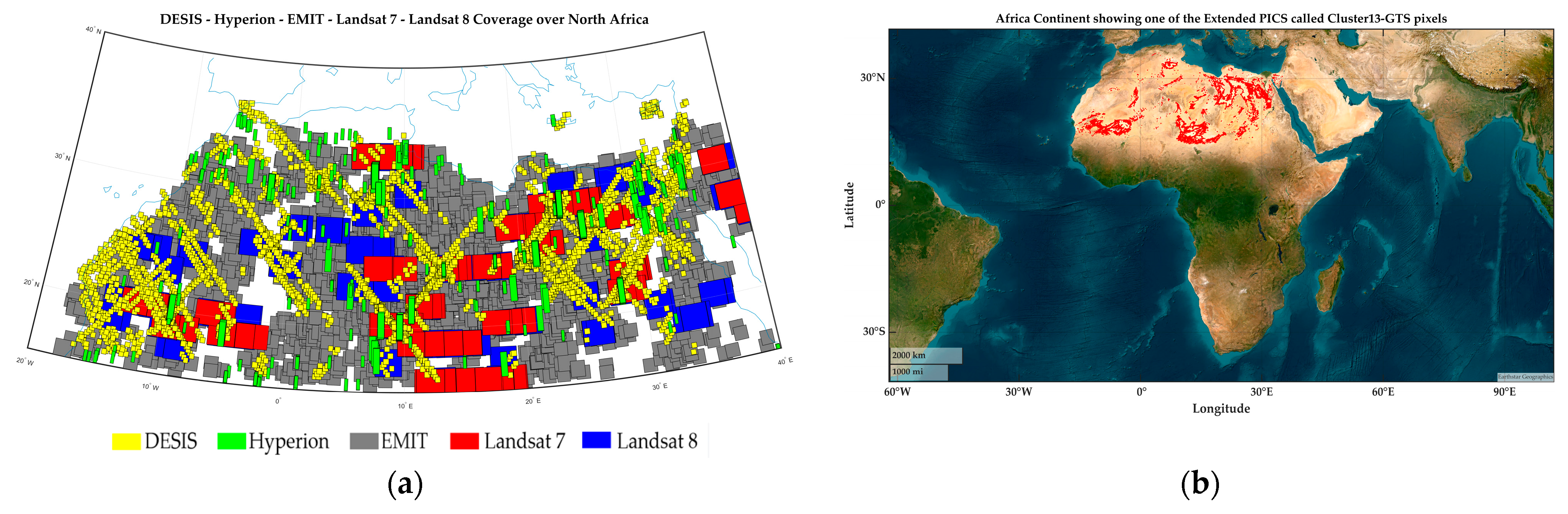
The section below gives insight into all the sites used in this paper, discussing why these were selected and what makes EPICS different from PICS. The sites used in the paper are a cluster from the EPICS classification named Cluster13–GTS, four RCN sites, two South Dakota State University (SDSU) sites, Algodones Dunes (AD), and Lake Tahoe (LT).

Cluster13–GTS over North Africa

Traditionally, PICS was used in processes like post-launch radiometric calibration, sensor stability monitoring, validation, etc., due to their homogeneity and temporal stability. However, studies have been conducted on temporal stability analysis on PICS sites. One such study by Khadka, N. et al. [24] assessed the temporal stability of PICS sites by identifying change points in the time series collected by OLI, ETM+, MODIS, and Sentinal–2A. As a result, statistical trends were identified in those PICS sites. Due to these site trends, detecting and correcting sensor drift becomes more challenging, leading to false trends or over–correction. As specified earlier, this was one of the potential drawbacks of the Hyperion lifetime calibration process conducted by Jing, X. et al. [23]. Another potential drawback of using PICS was data limitation, especially in sensors on ISS, due to the lack of a revisit cycle. This makes it difficult to find enough data points to analyze the time series. Given those limitations in PICS usage for radiometric calibration, finding different temporally stable regions globally for calibration becomes essential. Using temporally stable areas is a crucial factor for the radiometric calibration of optical sensors in remote sensing. Studies are performed to find temporally stable regions to replace PICS.

The research conducted by Fajardo et al. [43] focuses specifically on temporally stable pixel identification using statistical tests for change point and long-term trend detection. The author has analyzed beyond desert sites, covering global regions with broad spectral characterization to identify areas useful in the stability monitoring and radiometric calibration of optical sensors. The author has generated a global mosaic consisting of those temporally stable pixels. In other research conducted by the same author, Fajardo et al. [30] used the global mosaic generated in a previous paper as a base for the clustering process performed employing a K–means clustering algorithm. The author classified the stable temporal pixels into 160 clusters by grouping pixels that have similar temporal and spectral characterization as one cluster. This clustering was called Extended Pseudo Invariant Calibration Sites (Extended PICS or EPICS). Along with identification and classification, the author has also performed the validation of EPICS for their potency for calibration, which is a crucial step using Cluster160, as this cluster included the pixels from one of the RCN sites, GONA. The author used this cluster for validation as it was possible to validate directly using RCN TOA reflectance derived from ground measurements.

Among the EPICS, the cluster used in this work is Cluster13–GTS, as those have similar spectral characterization to that of the PICS sites Libya4, a bright sand target. Figure 2b shows the temporal stable pixel distribution of Cluster13–GTS over North Africa and the data in the IPLAB archive for all the sensors over the same region. However, this Cluster13–GTS from EPICS 160 clusters was not validated.

RCN Sites

Radiometric Calibration Network (RadCalNet or RCN) is an effort to facilitate vicarious reflectance–based calibration for optical sensors by automating and providing in–situ surface and atmosphere data (ground truths) as a part of a network, including multiple sites for the radiometric calibration of optical sensors from VNIR to SWIR spectral ranges. The main objective of RCN is to standardize protocols for collecting data, process to top–of–atmosphere reflectance, and provide uncertainty budgets for automated sites traceable to the international system of units. RCN is a result of the RCN Working Group under the umbrella of the Committee on Earth Observation Satellites (CEOS) Working Group on Calibration and Validation (WGCV) and the Infrared Visible Optical Sensors (IVOS) [12]. Currently, there are five radiometric calibration instrumented sites: Railroad Valley Playa located in the USA (RVUS), La Crau in France (LCFR), Baotou sand site in China (BSCN), and Gobabeb in Namibia (GONA), and an artificial site in China (BSTN) that is not used in this work.

All the sites collect their surface reflectance data, atmospheric data, which are later converted to TOA reflectance data with their associated uncertainties on a hyperspectral scale from 400 nm to 2500 nm with a spectral resolution of 10 nm following a standard procedure for all the sites, except for BSCN, which goes only to 1000 nm. These data are made available to users in the RCN portal. RCN collects the data every 30 min in intervals between 9:00 AM and 3:00 AM in their local time over nadir-viewing geometry. Detailed processes followed for predicting TOA reflectance based on a radiative transfer code (MODTRAN) using surface reflectance and estimating the uncertainty budget are mentioned in the RCN paper by Bouvet, M. et al. [12]. This paper also provides ROI sizes for each site (the ROI size used for each sensor calibration is provided in their respective sections in the Methodology). The TOA reflectance with its uncertainties is provided in the level 1 data used for the work. The RCN–reported uncertainty for each site is RVUS 3.5–5.3%, LCFR 3.5–5%, BSCN 4–5%, and GONA 3.5–4% [44,45,46,47,48].

Before using RCN data, fill values (flags) in absorption bands (RCN does not provide measurements for those bands) and bands whose uncertainty was flagged were removed. Uncertainties for those bands are flagged with a negative sign specifying that one of the inputs is more significant than their respective look-up-table (LUT) interval [49]. Finally, for EMIT, due to its spatial resolution being 60 m and LCFR site ROI given to be a 30 m disk, a homogeneity evaluation was performed using OLI over LCFR, where the actual ROI was compared with the extended ROI. This was accomplished by comparing the mean TOA reflectance of all the measurements in a day for an actual ROI of 30 m with the extended ROI of 90 m on the same day for every OLI band. This was performed for all the available dates. Along with visual inspection showing that the mean of both the ROIs were within their uncertainties, a statistical test was performed to quantify the results. Based on the results, it was concluded that an extended ROI can be used for EMIT as they are homogenous.

Other Ground Truth Targets

Apart from RCN, other ground data over different sites were used for EMIT’s absolute calibration to resolve the data limitation caused by EMIT’s short orbital time. The dark water target Lake Tahoe (LT), bright sand target Algodones Dunes (AD), and two vegetative ROIs consisting of grass and soybean from SDSU sites were considered to utilize a variety of target types.

LT is a large, deep lake situated in a granite graben near the crest of the Sierra Nevada Mountains on the border of California and Nevada. As this is one of the high-water clarity lakes, it is an ideal radiometric and vicarious calibration test site under the EROS Cal/Val Center of Excellence (ECCOE) [50]. Due to its spectral response matching with deep water, the deep–water hyperspectral surface reflectance profile was used to predict the TOA reflectance of the required date. An ROI was created around the CEOS center Latitude and Longitude of N 39.00 and W 120.00 (in degrees), respectively.

As for Algodones Dunes (AD), a bright sand target, many field campaigns were performed during 2015 [11,51], and the ROI was selected based on knowledge of this work. For SDSU sites, the ground truths were measured for the required dates using an ASD [52] (site images are provided in this paper). The ASD measurements for AD and SDSU sites were processed following the steps discussed in the paper under the ASD FieldSpec section by Pathiranage, D.S. et al. [52]. The surface reflectance from the processed ASD for AD and SDSU sites and the deep–water hyperspectral surface reflectance profile for LT was used to predict the TOA reflectance through a radiative transfer code (MODTRAN 5).

Libya4

Libya4 is the most–often used PICS site due to its high radiometric stability and size. This bright desert site is in the Great Sand Sea in North Africa, made of sand dunes with no vegetation. The CEOS ROI with center latitude and longitude of N 28.00 and E 23.39 (in degrees) [53] was used to compare two versions of the Hyperion calibration.

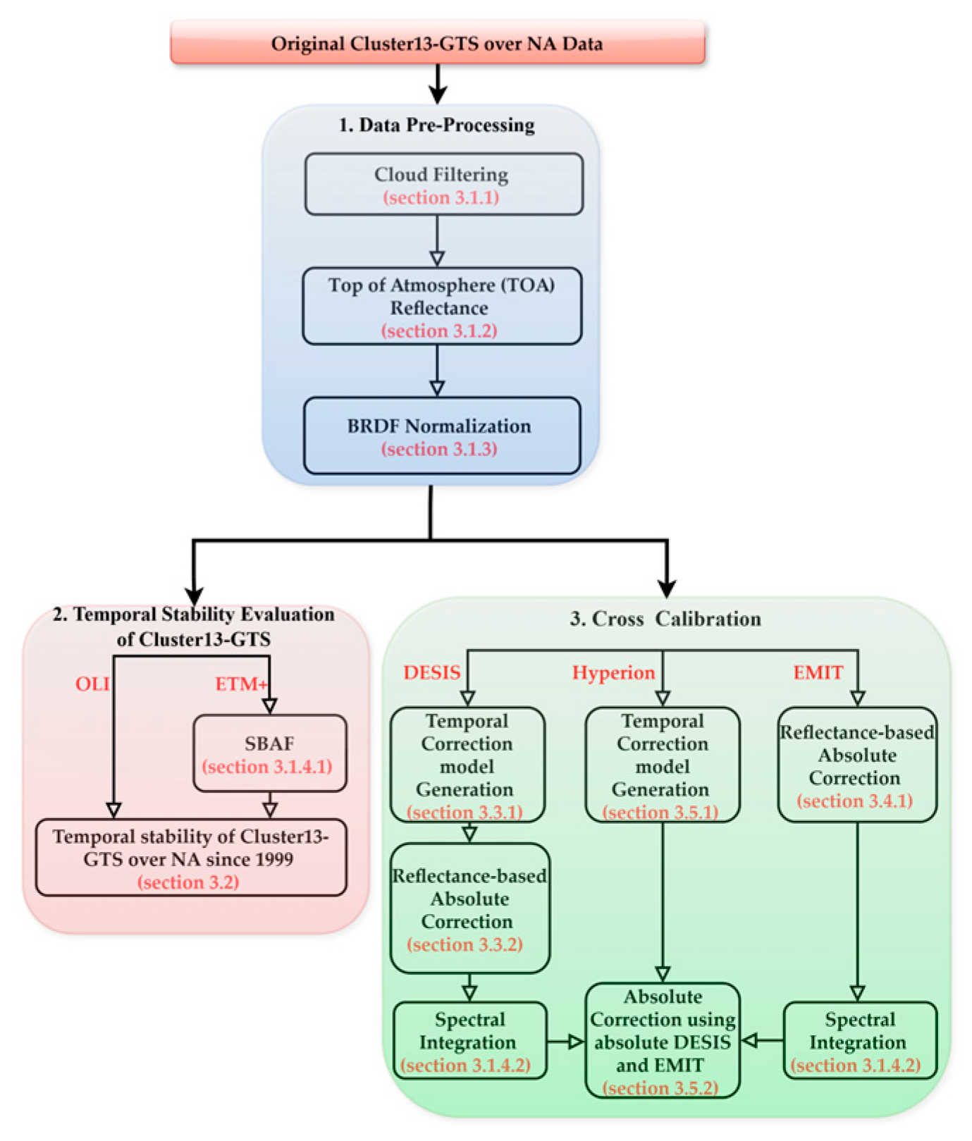
2.2. Methods

The methodology enables the combination or integration of all of these sensors, providing enhanced temporal, spatial, and spectral coverage, which helps with the land surface characterization on a hyperspectral scale. The flowchart in Figure 3 outlines the key steps involved in the process. The first box shows the data pre-processing, and the second box shows the steps followed for the temporal stability monitoring of Cluster13-GTS used for calibration and validation. Finally, the third box shows the steps involved in calibrating hyperspectral sensors. This section provides a detailed explanation of each step. This section contains the following subsections explaining the approach:

• Data Pre-processing
• Temporal Stability Evaluation of Cluster13–GTS since 1999
• Vicarious Calibration of DESIS
• Vicarious Calibration of EMIT
• Cross-Calibration of Hyperion using Absolute DESIS and EMIT
• Validation of Calibration Coefficients
• Uncertainty Analysis
• Statistical Tests

2.2.1. Data Pre–Processing

After selecting the sites required for the work, the images extracted from all the sensors must undergo pre–processing before their actual use in cross–calibration. This section briefly discusses those steps from the flowchart (inside the blue box) mentioned under pre–processing as an individual subsection.

Cloud Filtering

Cloud filtering was conducted across all sensors to remove cloud–affected pixels, ensuring minimal cloud interference. In addition to achieving minimal cloud cover for scene retrieval from their respective websites for each sensor, the study actively filtered out the cloud–affected pixels from the images using various techniques. For the Landsat series, ETM+, and OLI, the cloud filtering was based on the BQA band, while for hyperspectral sensors, Hyperion, DESIS, and EMIT filtering used a threshold–based approach. The threshold was determined by analyzing the spectral response of the bright, invariant target Cluster13–GTS in a specific water absorption band. This band was selected using the atmospheric transmittance curve shown in Figure 4 as a reference.

This study used atmospheric transmittance generated using Modtran to identify the water absorption bands. Atmospheric gases, like water vapor, ozone, carbon dioxide, etc., influence the curve’s structure through molecular absorption [54]. The proper band for cloud filtering was selected based on the identified water absorption bands. In this paper, specific water absorption bands and the required threshold for each hyperspectral sensor are based on their spectral resolution. The following subsections briefly describe the cloud filtering process for each sensor.

• DESIS

The DESIS instrument records images in the VNIR region (400 nm to 1000 nm) with a spectral resolution of ~2.55 nm [28]. The water absorption band around 900 nm to 1000 nm is a broad absorption feature in the DESIS spectral range. Due to its narrower spectral sampling, DESIS is more sensitive to the absorption feature associated with clouds at that spectral range.

The study used a TOA reflectance threshold of 0.2 at the 934.5 nm water absorption band to identify cloud–affected pixels (determining that any value more significant than the threshold is an affected pixel). The process then applied the resulting binary cloud mask to remove cloud–affected pixels from all the images.

Figure 5a depicts a DESIS image over Libya4, part of Cluster13–GTS, potentially containing clouds and cloud shadow. Figure 5b represents the same image in the 934.5 nm absorption band, with a corresponding color bar. As explained earlier, based on atmospheric transmittance, cloud–contaminated pixels in the true–color image exhibit a reflectance of 0.2 or higher in the absorption band image. In contrast, surface or unaffected pixels typically reflect less than 0.2 in that particular band due to water absorption. Therefore, as explained before, a threshold of 0.2 was applied to identify and filter cloud–affected pixels from the scenes. Figure 5c shows the resulting cloud–filtering mask, where white areas indicate the cloud–affected pixels, while black areas represent cloud–free regions. The study follows an exact process for both Hyperion and EMIT for the threshold setting.

2.

Hyperion

The Hyperion instrument records images in the VNIR region (400 nm to 1000 nm) and the SWIR region (900 nm to 2500 nm) with a spectral resolution of ~10 nm [18]. The water absorption band, around ~1300 nm to 1500 nm, is one of the absorption features in the Hyperion spectral range. The spectral region is highly susceptible to atmospheric absorption. Therefore, this section selected the wavelength 1386.7 nm at the dip of absorption region due to its narrowness and alignment with Hyperion’s spectral sampling.

A TOA reflectance threshold of 0.02 at 1386.7 nm identified cloud–affected pixels (those exceeding the threshold). The resulting binary cloud mask subsequently removed cloud–contaminated pixels from all images.

3.

EMIT

The EMIT instrument observes a spectrum ranging from 380 nm to 2500 nm with a sampling of ~7.4 nm [29]. Like Hyperion, this study selected the wavelength 1387 nm at the absorption band’s dip as the water absorption band. A TOA reflectance threshold of 0.02 at this specific wavelength identified cloud–affected pixels (those exceeding the threshold). The resulting binary cloud mask subsequently removed cloud–contaminated pixels from all images.

4.

Landsat series

For ETM+ and OLI products, the pixel–quality–assessment band (QA_PIXEL) was used to generate a cloud filtering mask. The mask is based on bit information provided by USGS Landsat Collection 2 Quality Assessment Bands (https://www.usgs.gov/landsat-missions/landsat-collection-2-quality-assessment-bands (accessed on 20 February 2024) within the band, which includes bit 0 (fill value), bit 1 (dilated cloud), bit 2 (cirrus), bit 3 (cloud), bit 4 (cloud shadow), bit 9 (cloud confidence), bit 11 (cloud shadow confidence), and bit 15 (cirrus confidence). This cloud–filtering mask was applied to all the images to remove cloud–affected pixels [55].

TOA Reflectance Computation

The next step after cloud filtering is converting DN or at–sensor radiance to TOA reflectance to provide a consistent unit; in this case, TOA reflectance units match NIST traceability. This section explains how TOA reflectance is obtained for individual sensors used in the process.

For the hyperspectral sensors, Hyperion, DESIS, and EMIT, the TOA reflectance for each wavelength is calculated as follows:

$${\rho }_{\lambda }={\displaystyle \frac{\pi \ast L_{\lambda }\ast d^2}{E_{SUN,\lambda }\ast \mathit{cos}\left({\theta }_{SZA}\right)}},$$

(1)

where ${\rho }_{\lambda }$ corresponds to TOA spectral reflectance in reflectance units, $L_{\lambda }$ is the at–sensor spectral radiance whose units are sensor–specific, $E_{SUN,\lambda }$ is the solar exoatmospheric irradiance obtained from the Thuillier model [56] in $\mathrm{m}\mathrm{W}{\mathrm{m}}^{-2}\mathrm{n}{\mathrm{m}}^{-1}$, $d$ is the EarthSun distance in astronomical units, and ${\theta }_{SZA}$ is the solar zenith angle in degrees.

• DESIS

The DESIS product used for this work was in a 16–bit integer scaled DN format. DN to spectral radiance conversion was performed using gain and offset scaling factors for each band provided in the product metadata file. The radiance conversion is done using the below Equation (2) [31].

$$L_{\lambda }=G_{\lambda }\ast D{N}_{\lambda }+O_{\lambda },$$

(2)

where $L_{\lambda }$ is the spectral radiance in $\mathrm{m}\mathrm{W}\mathrm{c}{\mathrm{m}}^{-2}\mathrm{s}{\mathrm{r}}^{-1}\mathsf{\mu }{\mathrm{m}}^{-1}$ [31], $G_{\lambda }\mathrm{a}\mathrm{n}\mathrm{d} O_{\lambda }$ are the gain (multiplicative) and offset (additive) scaling factors, and $D{N}_{\lambda }$ is the recorded numerical values (DNs) of electromagnetic energy at each pixel.

TOA reflectance conversion from spectral radiance was performed using Equation (1), before which the units should be consistent. To achieve that, spectral radiance was multiplied by 10 to match the solar irradiance units. Angular information ${\theta }_{SZA}$ was obtained from the product’s metadata.

2.

Hyperion

Unlike DESIS, the Hyperion image data in DN were converted to spectral radiance by applying the scaling factor given in the product metadata in Equation (3) [19]. There are two scaling factors in the metadata, one for all VNIR wavelengths and the other for all SWIR wavelengths. Based on the band scaling factor, it is applied to obtain spectral radiance from DN.

$$L_{\lambda }={\displaystyle \frac{D{N}_{\lambda }}{scaling factor}},$$

(3)

where $L_{\lambda }$ is the spectral radiance in $\mathrm{W}{\mathrm{m}}^{-2}\mathrm{s}{\mathrm{r}}^{-1}\mathsf{\mu }{\mathrm{m}}^{-1},$ the scaling factors 40 and 80 for VNIR and SWIR, respectively [19], and $D{N}_{\lambda }$ is the recorded numerical values (DNs) of electromagnetic energy at each pixel.

TOA reflectance conversion from spectral radiance was performed using the Equation (1). Solar Zenith Angular (SZA) information was estimated by subtracting the solar elevation angle provided in the product metadata.

3.

EMIT

The EMIT product used in the process is at–sensor radiance. TOA reflectance was computed using Equation (1). The EMIT at–sensor radiance is in $\mathsf{\mu }\mathrm{W}\mathrm{c}{\mathrm{m}}^{-2}\mathrm{s}{\mathrm{r}}^{-1}\mathrm{n}{\mathrm{m}}^{-1}$ [37]. To make it consistent with solar irradiance and use it in Equation (1), the at–sensor radiance was multiplied by 10. Geometrical angular information and the Earth–Sun distance are pixel–based information from the product’s Observation Geometric File (OBS).

4.

Landsat series

For ETM+ and OLI, DN–to–TOA reflectance was obtained using Equation (4) provided by the USGS Landsat Level1 Data Product (https://www.usgs.gov/landsat-missions/using-usgs-landsat-level-1-data-product (accessed on 20 February 2024).

$${\rho }_{\lambda }= {\displaystyle \frac{M_{\lambda }\ast D{N}_{\lambda }+A_{\lambda }}{\mathit{cos}\left({\theta }_{SZA}\right)}},$$

(4)

where $M_{\lambda }, A_{\lambda }$ are the multiplicative and additive scaling factors that are provided in the metadata of the level 1 collection 2, $D{N}_{\lambda }$ is the recorded numerical values (DNs) of electromagnetic energy at each pixel, and solar angular information was obtained from the solar angle products.

BRDF Normalization

Earth–observing sensor measurements are influenced by illumination geometry, acquisition view geometry, and atmospheric effects, leading to variability in their TOA reflectance. Varying solar angles cause the sensor to view the target uniquely every time. Over time, this causes the seasonal effect in the time series data, as shown in Figure 6a. Thus, the varying solar position over seasons significantly contributes to the bidirectional reflectance distribution function (BRDF). Unlike Landsat sensors and Hyperion in the polar sun–synchronous orbit, DESIS and EMIIT have varying view geometries due to their deployment on ISS, which further contributes to the bidirectional reflectance distribution function (BRDF) [17]. A 4–angle empirical BRDF model developed at SDSU IPLab [17] was utilized to remove the BRDF effect from TOA reflectance. 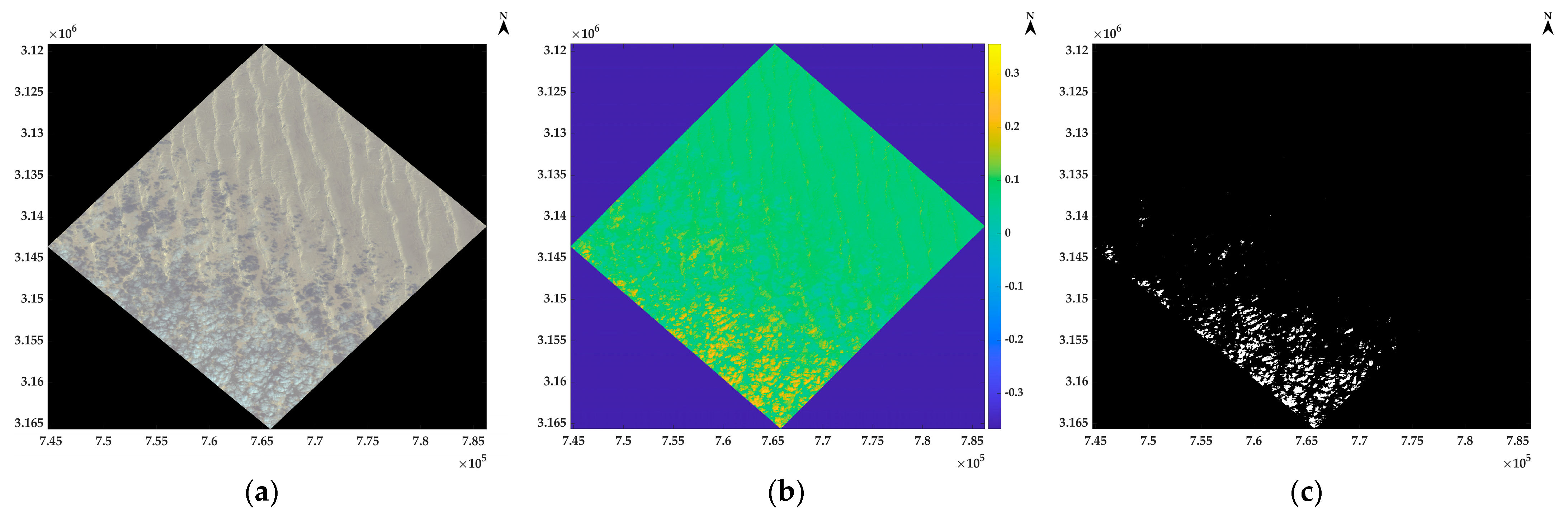The 4–angle BRDF model (Equation (5)) was derived for individual bands (across the sensors spectral range) using cloud–filtered TOA reflectance Cluster13–GTS data for each sensor along with their angular information (provided with the sensor product) in its Cartesian form (Equation (6)).

$$\begin{gathered} {\rho }_{BRDF,predicted} = {\beta }_0+{\beta }_1{X}_1+{\beta }_2{Y}_1+{\beta }_3{X}_2+{\beta }_4{Y}_2+{\beta }_5{X}_1{Y}_1+{\beta }_6{X}_1{X}_2+{\beta }_7{X}_1{Y}_2+{\beta }_8{Y}_1{X}_2+ \\ {\beta }_9{Y}_1{Y}_2+{\beta }_{10}{X}_2{Y}_2+{\beta }_{11}{X}_1^2+{\beta }_{12}{Y}_{1 }^{2 }+{\beta }_{13}{X}_2^2+{\beta }_{14}{Y}_{2 }^{2 } , \end{gathered}$$

(5)

where, ${\beta }_0\mathrm{ }\mathrm{to}\mathrm{ }{\beta }_{14}$ are the coefficients of the model, $X_1,\mathrm{ }{X}_2,\mathrm{ }{Y}_1,\mathrm{a}\mathrm{n}\mathrm{d}\mathrm{ }{Y}_2$ are the angular information in Cartesian coordinates, and ${\rho }_{BRDF,predicted}$ stands for the model–predicted TOA reflectance. Angular information in sensor products is typically in spherical coordinates, which were converted to Cartesian coordinates using the following equations:

$$\begin{gathered} Y_1=\mathit{sin}\left(SZA\right)\ast \mathit{sin}\left(SAA\right) Y_2=\mathit{sin}\left(VZA\right)\ast \mathit{sin}\left(VAA\right) \\ {X}_1=\mathit{sin}\left(SZA\right)\ast \mathit{cos}\left(SAA\right) X_2=\mathit{sin}\left(VZA\right)\ast \mathit{cos}\left(VAA\right) \end{gathered}$$

(6)

where SZA and SAA represent the solar zenith and solar azimuth angles, and VZA and VAA correspond to the view zenith and view azimuth angles. The observed TOA reflectance was then normalized using a set of reference/normalizing angles. These normalizing angles were selected using polar plots (Figure 6b,c), prioritizing the consistency between the sensors and the lowest view geometry possible (considering the sensors on ISS having a broader view geometry). The normalized angles (represented in the black markers in the figure) used in the BRDF normalization process for all the sensors are shown in

Table 1. Normalizing angles used for BRDF normalization of all the sensors used in the work over Cluster13–GTS.

Sensors/Angles	Solar Azimuth (SAA)	Solar Zenith (SZA)	View Azimuth (VAA)	View Zenith (VZA)
DESIS	154.9°	46.2°	−120.3°	3.1°
EMIT	149°	46.9°	113.7°	3.3°
Hyperion	147.9°	44.3°	98°	3.4°
ETM+	150.6°	47°	101.7°	3.5°
OLI	154.8°	45.6°	111.1°	3.2°

. The equation below was used to obtain the BRDF–normalized TOA reflectance

$${\rho }_{\lambda ,BRDF Normalized}={\displaystyle \frac{{\rho }_{\lambda ,reference}}{{\rho }_{\lambda ,predicted}}}\times {\rho }_{\lambda ,observed},$$

(7)

where ${\rho }_{\lambda ,BRDF Normalized}$ represents the BRDF–normalized TOA reflectance, ${\rho }_{\lambda ,reference}$ corresponds to the TOA reflectance at a set of normalizing angles, ${\rho }_{\lambda ,predicted}$ represents the BRDF model–predicted TOA reflectance, and finally, ${\rho }_{\lambda ,observed}$ corresponds to the observed TOA reflectance (cloud filtered).

Figure 6a–c below present an example of the original OLI time series showing the seasonal effect and a polar plot illustrating the angular geometry distribution for DESIS and EMIT on the ISS, OLI, Hyperion, and ETM+ on a polar sun–synchronous orbit. BRDF normalizing angles were selected using the polar plots shown in the figure below, prioritizing the consistency between the sensor and the lowest view geometry possible, as sensors on ISS have a broader view geometry.

Normalization of Spectral Difference

Earth–observing sensors operate within a specific spectrum range, causing variations in their view. To achieve cross–comparison or cross–calibration between sensors or combining them for applications, spectral response differences should be considered to ensure consistency. The sensor’s spectral response is represented by its RSR [15]. The spectral difference between sensors is shown in the Figure 7 below. The present section explains the techniques used to normalize these spectral differences.

• SBAF

For a multispectral–to–multispectral sensor comparison or calibration, SBAF is applied to compensate for their spectral differences. SBAF is calculated as the ratio of the simulated reflectance from a pair of sensors, as seen in the equation below:

$$SBAF={\displaystyle \frac{{\rho }_{\lambda ,\left(ref\right)}}{{\rho }_{\lambda ,\left(cal\right)}}}={\displaystyle \frac{\frac{\int {\rho }_{\lambda }\times RS{R}_{\lambda ,\left(ref\right)}d\lambda }{\int RS{R}_{\lambda ,\left(ref\right)}d\lambda }}{\frac{\int {\rho }_{\lambda }\times RS{R}_{\lambda ,\left(cal\right)}d\lambda }{\int RS{R}_{\lambda ,\left(cal\right)}d\lambda }}},$$

(8)

where ${\rho }_{\lambda \left(ref\right)},\mathrm{a}\mathrm{n}\mathrm{d}\mathrm{ }{\rho }_{\lambda \left(cal\right)}\mathrm{ }$ represent the simulated TOA reflectance of both the reference and calibration sensors, respectively, and ${\rho }_{\lambda }$ corresponds to the hyperspectral profile. The simulated TOA reflectance is obtained by integrating the hyperspectral profile within the sensor’s RSR bandwidth and dividing it by its integrated RSR [15]. The SBAF is then applied to the uncalibrated sensor to achieve spectral consistency with the reference sensor:

$${\rho }_{\lambda ,\left(cal\right)}^{\prime }={\rho }_{\lambda ,\left(cal\right)}\times SBAF,$$

(9)

The implementation of SBAF is explained in Section 2.2.2.

2.

Spectral Integration

Unlike multispectral–to–multispectral, spectral integration is used to compensate for spectral differences between multispectral–to–hyperspectral, hyperspectral–to–multispectral, and hyperspectral–to–hyperspectral sensors, and spectral integration is used to compensate for their spectral difference. Spectral integration is performed using the following equation:

$${\rho }_{\lambda ,\left(ref\right)}^{\prime }={\displaystyle \frac{\int {\rho }_{\lambda ,\left(ref\right)}{RSR}_{\lambda ,\left(cal\right)}d\lambda }{\int {RSR}_{\lambda ,\left(cal\right)}d\lambda }},$$

(10)

where ${\rho }_{\lambda ,\left(ref\right)}^{\prime }$ corresponds to the TOA reflectance of the reference sensor spectrally consistent with the to–be–calibrated sensor. The reference and to–be–calibrated sensors can be interchangeable based on the application. The usage of spectral integration in this work is explained in future sections.

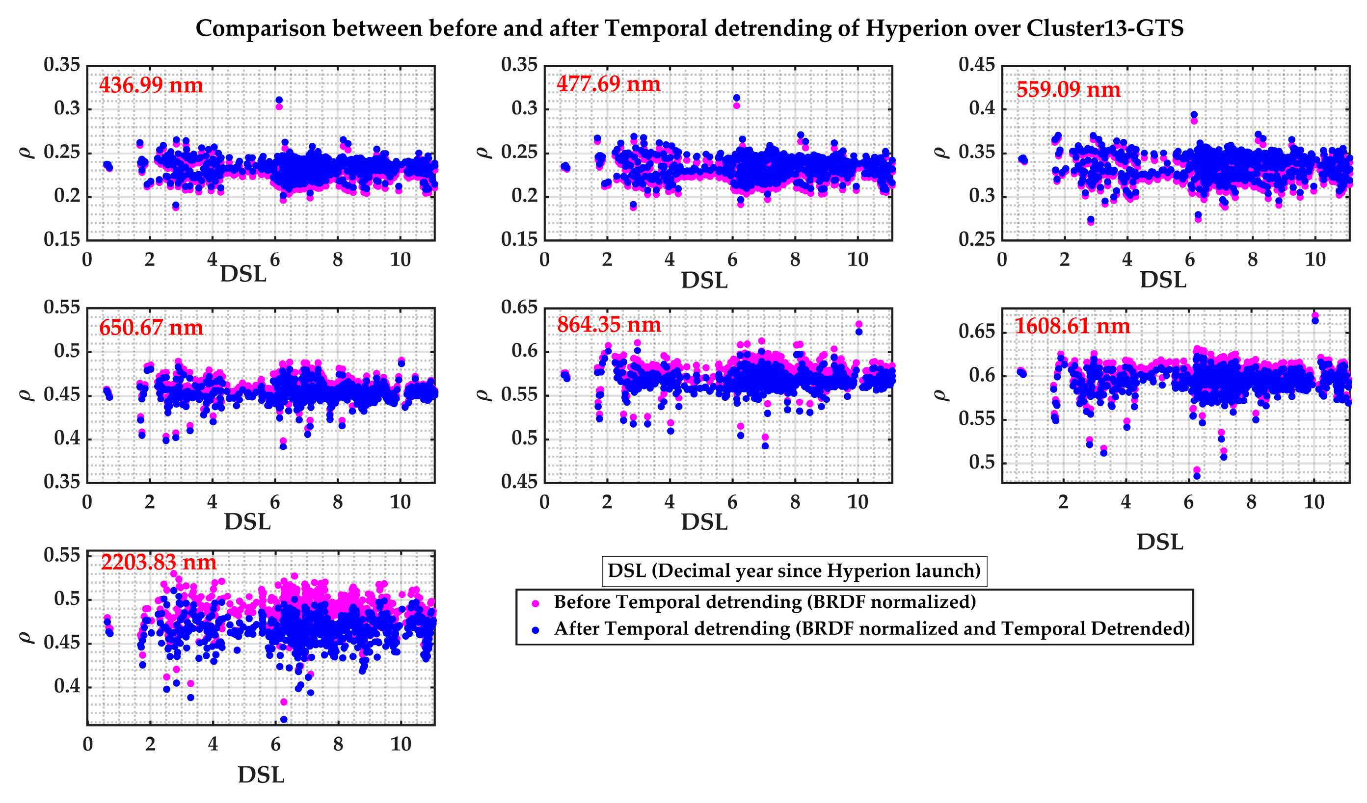
2.2.2. Temporal Stability Evaluation of Cluster13–GTS Since 1999

As described in Section Cluster13–GTS over North Africa, the Cluster13–GTS [30] was not validated; another key point was the use of this cluster from late 1999 to 2024 in this work made it necessary to evaluate the Cluster13–GTS temporal stability for the entire time frame. This study utilized ETM+ and OLI to assess the temporal stability for Cluster13–GTS from 1999 to 2024.

The analysis utilized 49 and 44 path/row combinations of ETM+ and OLI intersecting with Cluster13–GTS over North Africa, respectively. After cloud–contaminated pixel removal from the images of both sensors using the cloud filtering mask generated in the cloud filtering Section Cloud Filtering, TOA reflectance was obtained from the DN in the image data as described in the TOA reflectance computation Section TOA Reflectance Computation. Finally, performing BRDF normalization from Section BRDF Normalization, a 3sigma filter was then applied to obtain outlier–free data for further analysis. The final dataset had 3305 and 8651 data points in ETM+ and OLI, respectively.

To achieve this goal of temporal stability evaluation, ETM+ was cross–compared with OLI, assuming that OLI was well calibrated. For cross–comparison of any sensor, their spectral difference should be considered, as mentioned in the Normalization of Spectral Difference Section Normalization of Spectral Difference. To compare ETM+ with OLI, the spectral difference between them was corrected using the spectral band adjustment factor (SBAF) correction described in the same section. SBAF was calculated following the process demonstrated by Fajardo et al. [57] using the hyperspectral profile of Cluster13–GTS, developed by Fajardo et al. [57]. The author has shown that when calculating SBAF, both uncertainties associated with the hyperspectral profile and RSRs of the sensors are taken using the Monte Carlo simulation approach.

In this approach, the hyperspectral profile and RSR of ETM+ and OLI, along with their uncertainties, were considered input data. The RSR of OLI and ETM+ was obtained from the USGS Spectral Characteristics Viewer (https://landsat.usgs.gov/spectral-characteristics-viewer (accessed on 2 May 2024). Unlike OLI, which comes with RSR uncertainties, ETM+ RSR does not include uncertainty; hence, the sensor’s design of absolute radiometric uncertainty of 5% was assigned for this work. The probability density function (PDF) of these inputs, which provides an opportunity to propagate the uncertainties, was generated and then fed into the mathematical model, Equation (8) (SBAF), through a Monte Carlo Simulation of 1000 iterations. The mean and standard deviation from the Monte Carlo iterations were considered the SBAF and the uncertainty on the SBAF.

The SBAF obtained was then multiplied with the BRDF–normalized ETM+ (3305 data points) following Equation (9), which gives BRDF–normalized ETM+ data over Cluster13–GTS spectrally matching OLI, which is called simulated ETM+ in the future sections. The total uncertainty for both sensors was estimated before the actual temporal stability analysis. These uncertainties were calculated using the ISO Guide to the Expression of Uncertainty in Measurement (GUM) methodology [58]. The Uncertainty Equations (11) and (12) were used for ETM+ and OLI, respectively.

$$U_{total,ETM+}^2=\sqrt{U_{target}^2+U_{BRDF}^2+U_{SBAF}^2+U_{sensor}^2},$$

(11)

$$U_{total,OLI}^2=\sqrt{U_{target}^2+U_{BRDF}^2+U_{sensor}^2},$$

(12)

Here, $U_{total,ETM+}^2$ was considered as uncertainty on simulated ETM+, and $U_{total,OLI}^2$ as uncertainty on OLI BRDF–normalized TOA reflectance. In this analysis, $U_{target}^2$ was considered as a temporal coefficient of variation CV obtained by taking the ratio of the temporal std and mean (%), which includes temporal and spatial variability of the site (in future sections, this will be referred to as temporal CV). The BRDF model error or RMSE (Root Mean Square Error) measuring the difference between observed and model–predicted TOA reflectance is represented by $U_{BRDF}^2$ (in future sections, this will be referred to as BRDF model uncertainty). $U_{sensor}^2$ represents absolute sensor radiometric uncertainties (5% for ETM+, 3% for OLI). Finally, $U_{SBAF}^2$ represents the uncertainty on the SBAF correction factor estimated through a Monte Carlo simulation mentioned above.

To evaluate the temporal stability of Cluster13–GTS from 1999 to 2024, simulated ETM+ and BRDF–normalized OLI data are subjected to a linear regression analysis through a Monte Carlo simulation with 1000 iterations (steps from [15] for the Monte Carlo approach were followed throughout this paper by changing the mathematical model as required). This approach allowed for the propagation of uncertainties (calculated above) associated with each data point and its corresponding value. Random samples were generated based on the primary inputs’ PDFs and propagated through a 1:1 linear regression model. A linear regression was conducted to determine the optimal parameters, considering the uncertainties associated with each data point. The slope, with its uncertainty obtained from the linear fit, is tested for statistical significance using the slope test explained in the statistical tests Section Slope Test. The linear regression and slope test were performed individually on ETM+ and OLI for their respective period from 1999–2012 for ETM+ and 2013–2024 for OLI.

Though the absolute value of ETM+ was observed to be within the uncertainty of OLI, ETM+ was scaled to match OLI’s absolute value, assuming OLI to be well–calibrated. This was performed to have Landsat sensors on the same absolute scale for subsequent processes, such as validation. The scaling factor was estimated and multiplied to simulate ETM+ using the equations below to make ETM+ consistent with the OLI absolute value.

$$ScalingFactor={\displaystyle \frac{{\rho }_{\lambda ,OLI}}{{\rho }_{\lambda ,simulatedETM+}}},$$

(13)

$${\rho }_{\lambda ,simulatedETM+}^{\prime }={\rho }_{\lambda ,simulatedETM+}\ast ScalingFactor,$$

(14)

where ${\rho }_{\lambda ,OLI}$ corresponds to the temporal mean of the BRDF–normalized OLI, ${\rho }_{\lambda ,simulatedETM+}$ corresponds to the temporal mean of BRDF–normalized simulated ETM+, and finally, ${\rho }_{\lambda ,simulatedETM+}^{\prime }$ corresponds to scaled BRDF–normalized simulated ETM+.

2.2.3. Vicarious Absolute Calibration of DESIS

An evaluation of the temporal stability of Cluster13–GTS performed in the previous Section 2.2.2 justifies that Cluster13–GTS is temporally stable in the DESIS life span, implying that the temporal trend seen (observed in the cross–comparison of hyperspectral sensors result depicted in Figure 1 under the introduction Section 1) in DESIS is not due to a change in the target over time but is sensor–specific. This evidences the need for time–dependent coefficients suggested by Carmona, E. et al. [35] mentioned in the sensor overview Section DESIS. Given the limitations in the vicarious calibration and the observed trend, it was resolved to perform the vicarious absolute calibration of DESIS before employing it to cross–calibrate Hyperion.

This section briefly explains the methodology developed to perform the temporal de–trending and vicarious calibration of DESIS on an absolute scale, which is later used in cross–calibrating Hyperion.

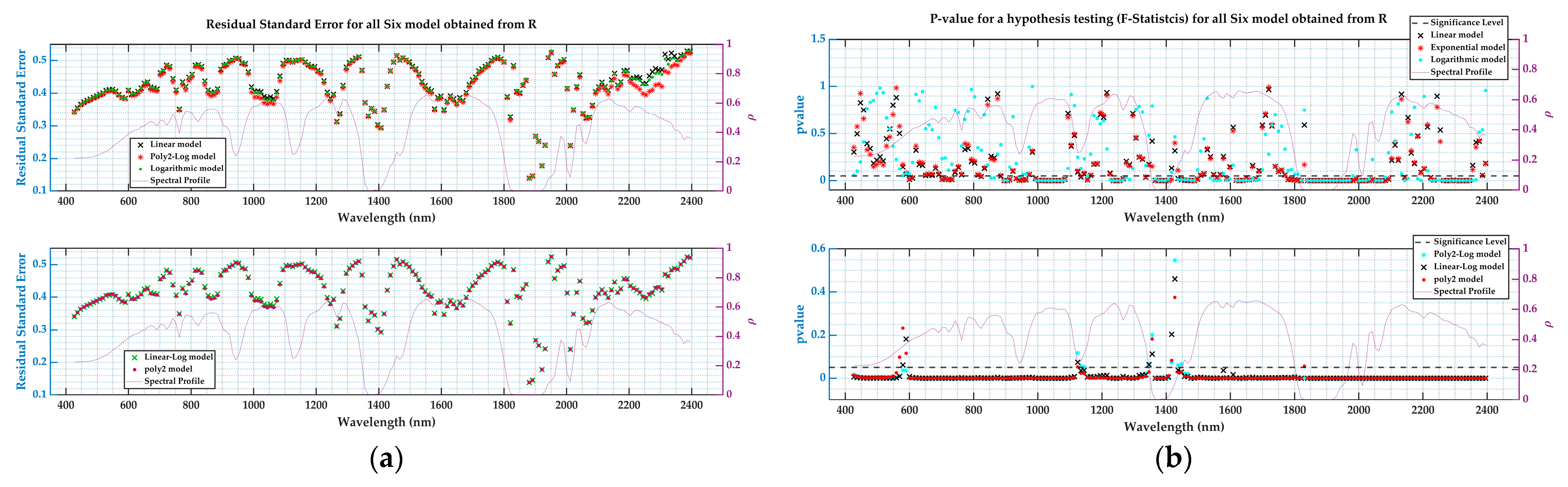
DESIS Temporal Correction Model Generation

Analyzing the nature of the trend was the first step in developing a de–trending model. This process uses DESIS images acquired over the Cluster13–GTS region, encompassing 1643 data points within the latitude and longitude boundaries seen in the data archive Figure 2a under sensor and site overview Section 2. The data requires preprocessing before being used in the temporal correction model generation. For that, clouds from the scenes were removed using the cloud filtering mask generated in cloud filtering Section Cloud Filtering, then converting DNs from the cloud–free scenes to TOA reflectance using Equation (1) from the TOA reflectance computation Section TOA Reflectance Computation. Normalizing the seasonality from the time series is crucial to catch any trend related to the temporal component; hence, BRDF normalization was performed as in the Section BRDF Normalization. With this preprocessed BRDF–normalized data, a temporal de–trending or correction model was developed.

The process uses statistical methods to select the best model through R. Four regression models were put into statistical testing: simple linear, exponential, 2nd–order polynomial (poly2), and 4th–order polynomial (poly4). These four models were chosen by visually inspecting the nature of the data. The model that satisfied the statistical criteria was considered the best de–trending model. The three criteria used in selecting the model were as follows [59,60,61]:

• Residual standard error (RSE): The smaller the residual standard error, the better the regression model fits the underlying data, meaning the error in the model’s prediction is minimum.
• F–Statistics and p–value: The F–score indicates how well the regression model describes the underlying data, in other words, how significant the model is. Suppose the p–value that corresponds to the F–score is less than 0.05. In that case, the regression model fits better, meaning the p–value tells how well the predictor variables are statistically worthy in predicting the output. So, overall, an f–score with a p–value of less than the selected significance (in this case 0.05) confirms that the regression model fits the underlying data well.
• Significance of the coefficients: This is calculated through the t–distribution on each coefficient in the model. This answers the question of which coefficient/predictor is statistically different than zero. If the p–value corresponding to the t–distribution is less than the 0.05 significance level, then the predictor variable is said to be significant to the model.

In summary, the first two criteria talk about the overall model, whereas the third criterion gives the knowledge about which coefficient has more influence on the model.

To statistically evaluate the regression model for temporal de–trending, BRDF–normalized TOA reflectance and a decimal year since DESIS launch were taken to be dependent and independent variables, respectively, along with which weights were included in the process as an uncertainty propagation in model generation. The weights in this process were the inverse square of uncertainty on BRDF–normalized TOA reflectance before correction. This uncertainty was estimated following the ISO Guide to the Expression of Uncertainty in Measurement (GUM) methodology [58]. The Uncertainty equation is as follows:

$$U_{BC}^2=\sqrt{U_{target}^2+U_{BRDF}^2},$$

(15)

Here, $U_{BC}^2$ was considered as uncertainty on BRDF–normalized TOA reflectance before correction, as mentioned in the temporal stability section, $U_{target}^2$ in this analysis was considered as temporal CV (%), and $U_{BRDF}^2$ was the BRDF model uncertainty. Both the uncertainties (cluster or target uncertainty and BRDF uncertainty) in this work are assumed to be independent suggesting the total uncertainty estimated may be slightly overestimated due to possibility of some interactions (dependency) between them (cluster or target uncertainty and BRDF uncertainty).

Finally, using the inputs mentioned above, the results from R were obtained for all the hyperspectral bands of DESIS. To summarize the R results, DESIS data were converted to multispectral to match OLI bands through Equation (10) from Spectral Integration in the Section Normalization of Spectral Difference. Regression was performed using those multispectral DESIS data in R. Based on the summarized R results for OLI spectral bands, it was observed the poly4 model consistently outperforming other models, exhibiting the lowest RSE across all the bands. While different models achieved higher F–scores, that alone makes it hard to select the model; the associated p–values were consistently low for the poly4 across all the bands, indicating a statistically significant fit to the underlying data. The same results were observed for hyperspectral bands. Consequently, this study adopted the 4th–order polynomial (poly4) model for the temporal de–trending of the DESIS data. The uncertainty in the temporal correction model was considered to be its RMSE, which measures the difference between BRDF–normalized TOA reflectance and model–predicted TOA reflectance, representing the model error.

Temporal de–trended data are obtained using following Equation (17).

$${\rho }_{\lambda ,\mathrm{p}\mathrm{r}\mathrm{e}\mathrm{d}\mathrm{i}\mathrm{c}\mathrm{t}\mathrm{e}\mathrm{d}}={\beta }_0+{\beta }_{1}X+{\beta }_2{X}^2+{\beta }_3{X}^3+{\beta }_4{X}^4,$$

(16)

$${\rho }_{\lambda ,tempDESIS}={\displaystyle \frac{{\rho }_{\lambda ,reference}}{{\rho }_{\lambda ,predicted}}}\times {\rho }_{\lambda ,BRDF NormalizedDESIS},$$

(17)

where ${\beta }_0-{\beta }_4$ are the coefficients of the poly4 model, whereas ${\rho }_{\lambda ,\mathrm{p}\mathrm{r}\mathrm{e}\mathrm{d}\mathrm{i}\mathrm{c}\mathrm{t}\mathrm{e}\mathrm{d}}$ is the model–predicted TOA reflectance, whereas X is the decimal year since launch, ${\rho }_{\lambda ,reference}$ is the predicted TOA reflectance at DESIS launch year (X = 0), and ${\rho }_{\lambda ,BRDF NormalizedDESIS}$ corresponded to the BRDF–normalized DESIS data, and finally ${\rho }_{\lambda ,tempDESIS}$ represents the temporal de–trended DESIS data.

DESIS Reflectance–Based Absolute Correction Using RCN

The temporal de–trending tends to shift the data from its absolute scale, making it necessary to perform an absolute correction to reverse the scaling to its actual value. The following section briefly explains the procedure used to estimate the correction factors required to calibrate the DESIS temporal de–trended data on an absolute scale. RCN was used as the ground reference to achieve this.

• DESIS data selection and filtering

DESIS images acquired at the coinciding and near–coinciding dates of RCN over RVUS, GONA, BSCN, and LCFR were used for this process. Apart from that, because DESIS is mounted on ISS, images acquired at a time outside the RCN time interval need to be filtered. Therefore, these two were the primary data–selection filters considered in this work. As explained in the Section BRDF Normalization, the BRDF effect, a factor influencing TOA reflectance, must be considered. Since only coinciding dates were chosen, the solar geometry for DESIS and RCN were similar. RCN measures in the nadir or views at the zenith of 0 degrees. Due to the ISS orbit, DESIS view angles vary. Hence, only DESIS images acquired at a view geometry <11 degrees were selected for further analysis [62]. The threshold was chosen based on the error percentage due to the view geometry difference seen between RCN and DESIS that goes into the process.

To estimate this error caused by the view geometry being different than nadir, meaning to evaluate the sensitivity of the target viewed at a different angle than zero degrees straight, the cosine of the angular difference between the DESIS view zenith and RCN view zenith (0 degrees) was used. In some applications, the cosine of the difference between two quantifies/values provides a measure of how sensitive the difference might be or provides an indication to the possible error due to the difference. The returned value is closer to 1, indicating a slight difference between the two values with minimal impact on the overall result. In this work, the cosine of the angular difference tells how much of an influence the view geometry deviation has on the target viewing. This uncertainty due to the view geometry difference was estimated using the following equation:

$$U_{VZA}=\mathit{cos}\left(VZ{A}_{DESIS}-VZ{A}_{RCN}\right),$$

(18)

Here, $U_{VZA}$ corresponds to the error due to the view zenith deviating from zero, and $VZ{A}_{DESIS}$ and $VZ{A}_{RCN}$ represent the DESIS view zenith and RCN view zenith, respectively, where the RCN view zenith ($VZ{A}_{RCN})$ is zero. Therefore, the 11 degrees was selected since it added ~1% uncertainty to the process. The clouds from the DESIS scenes were filtered using the cloud filtering mask generated for DESIS in the cloud filtering Section Cloud Filtering. After the cloud screening (the final filter), 64 data points of all RCN sites were used to estimate the absolute correction factor. The

Table 2. Showing the number of data points over each site used in DESIS’s absolute correction factor estimation.

Dates/Sites	RVUS	BSCN	GONA	LCFR
Coinciding	13	4	19	6
Near Coinciding	7	1	8	6
Total	20	5	27	12

below shows the number of coinciding and near–coinciding dates for individual sites.

2.

TOA Reflectance Extraction

• DESIS ROI TOA Reflectance Extraction:

After applying all the filters, the cloud–free scenes were used to extract the DESIS TOA reflectance from the ROI for all RCN sites used in the work. Due to DESIS GSD being 30 m, the ROIs given in the RCN site guide were used [44,45,46,47], intending the DESIS images over those ROIs to be obtained. An ROI size of 1 km × 1 km (~34 pixels × 34 pixels) for the RVUS site, 60 m × 60 m (~2 pixels × 2 pixels) for both GONA and LCFR sites, as they are a 30 m–diameter disk, and finally 300 m × 300 m (~10 pixels × 10 pixels) for the BSCN site were chosen according to the guide. Later, the TOA reflectance from the DNs in the ROI–intersecting area of DESIS images were extracted following the TOA computation of DESIS in the Section TOA Reflectance Computation.

Finally, the TOA reflectance over RCN ROIs was temporally de–trended through the temporal correction model developed in the Section DESIS Temporal Correction Model Generation.

• RCN TOA Reflectance Extraction for DESIS Comparison:

As mentioned in the site overview Section TOA Reflectance Computation, flag–free data were used for this work. The level 1 RCN data from those coinciding and near–coinciding dates mentioned earlier were utilized for further analysis before comparing them with DESIS. For the near–coinciding dates, an additional uncertainty was added to the actual uncertainty provided by the RCN following the ISO–GUM technique mentioned in the above sections. This uncertainty was estimated by evaluating the site variability within 24 h, meaning the percentage absolute difference in TOA reflectance within 24 h was considered the uncertainty due to the near–coinciding date. This uncertainty was added per band with the uncertainty provided in the RCN product for only those near–coinciding dates by using the equation below.

$${U^{\prime }}_{RCN}^2=\sqrt{U_{RCN}^2+U_{ncd}^2}$$

(19)

where ${U^{\prime }}_{RCN}^2$ corresponds to the total uncertainty on RCN for the near–coinciding dates, $U_{RCN}^2$ represents the uncertainty provided in the level 1 RCN product for the near–coinciding dates, and lastly, $U_{ncd}^2$ corresponds to the uncertainty estimated due to the site variability within 24 h. Overall, the uncertainty estimated due to near–coinciding date was 1.6–4% on the RVUS site, 1–3.5% on the GONA site, 2–4% on the LCFR site, and 2.5–4% on the BSCN site across the spectrum except for the deep absorption features.

Due to DESIS varying the acquisition time, the RCN measurements and their uncertainties on the measurements from the closest time intervals of the date were temporally interpolated. The overpass time was bracketed by the nearest time from the 30–min interval measurements on that date, meaning the closest time was selected as close as possible to the overpass time of DESIS. RCN data were temporally interpolated to match the DESIS overpass time using the linear model to account for variability in the DESIS acquisition time and RCN.

Finally, after the temporal interpolation, RCN data were spectrally interpolated to align with the DESIS spectrum, as it is the uncalibrated sensor and RCN is the reference. The data downscaling from 10 to 2.5 nm was performed using the makima technique. This technique was chosen after comparing its performance to spline and pchip interpolation methods using the original 1 nm RCN data from the RVUS site. First, the 1 nm data were averaged every 10 nm to obtain the pseudo 10 nm spectral resolution data, followed by spectral interpolating the pseudo 10 nm data back to 1 nm using the three methods: makima, pchip, and spline. The makima method preserved the spectral shape of the underlying data while minimizing the mean absolute error, mean square error, and root mean square error. Hence, the makima technique was used to interpolate RCN data to match the DESIS spectrum spectrally. Like temporal interpolation, spectral interpolation was performed on both temporally interpolated RCN TOA reflectance and their respective uncertainties.

3.

DESIS Gain Calculation

After TOA reflectance extraction from DESIS and RCN, this work performed a one–to–one comparison considering the uncertainties. The uncertainty on DESIS ROI TOA reflectance after temporal de–trending was attributed to the combined uncertainty of the view geometry difference and temporal correction model uncertainty. This uncertainty was combined through ISO–GUM, as mentioned in the earlier sections following Equation (20) below. The RCN uncertainty includes the uncertainty provided in the RCN product for coinciding dates and the uncertainty ${U^{\prime }}_{RCN}^2$ from the above RCN TOA reflectance extraction for near–coinciding dates.

$$U_{DESIS,VCD}^2=\sqrt{U_{TCM}^2+U_{VZA}^2},$$

(20)

where $U_{DESIS,VCD}^2$ represents the total uncertainty on DESIS over Vicarious Calibration Data (VCD in this case over RCN Sites), $U_{TCM}^2$ represents the uncertainty on the temporal correction model, and finally, $U_{VZA}^2$ corresponds to the uncertainty due to the view geometrical difference obtained from Equation (18).

To estimate the absolute correction factor, the work performed a 1:1 linear fit between DESIS and RCN data incorporating the weights using a Monte Carlo technique with 1000 iterations. This approach allowed for the propagation of the uncertainties on each data point with its TOA reflectance value. Random samples were generated based on the primary inputs’ PDFs and propagated through a 1:1 linear regression model. A weighted 1:1 linear regression was used to determine the optimal correction factor, considering the uncertainties associated with each data point. For the 1:1 linear regression, bias is assumed to be zero as the DESIS instrument has a dark current measurement on board. The absolute correction factor/gain was estimated as the mean of slope values obtained through the Monte Carlo simulation and the standard deviations of those slope values as the uncertainty on the gain.

Finally, the gain and its uncertainty can be used to correct the temporal de–trended DESIS data using the equation below.

$${\rho }_{\lambda ,absDESIS}={\rho }_{\lambda ,tempDESIS}\ast gai{n}_{\lambda },$$

(21)

where ${\rho }_{\lambda ,absDESIS}$ corresponds to temporal de–trended, absolute corrected DESIS TOA reflectance, ${\rho }_{\lambda ,tempDESIS}$ represents the temporal de–trended DESIS TOA reflectance, and gain is the absolute correction factor estimated using Monte Carlo 1:1 linear regression.

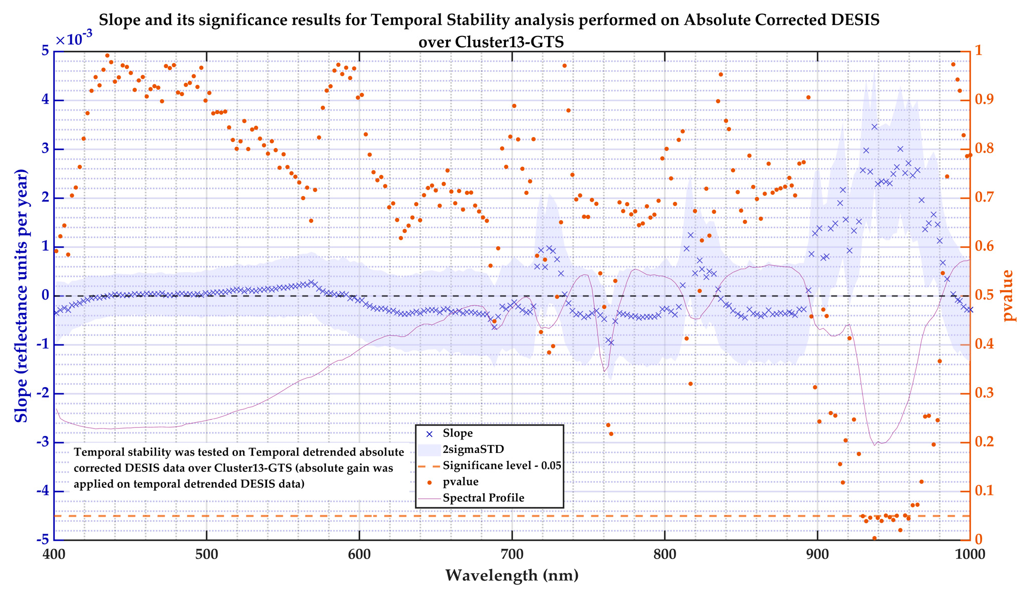
DESIS Statistical Test for Linearity Check After Temporal De–Trending

The gain estimated in the previous section was later applied to the BRDF–normalized, temporal de–trended DESIS data (${\mathsf{\rho }}_{\mathsf{\lambda },\mathrm{t}\mathrm{e}\mathrm{m}\mathrm{p}\mathrm{D}\mathrm{E}\mathrm{S}\mathrm{I}\mathrm{S}}$) over Cluster13–GTS to obtain the BRDF–normalized, temporal de–trended, absolute corrected DESIS data (${\rho }_{\lambda ,absDESIS}$). A statistical test was performed to validate the temporal correction performed. To achieve that, the same process described in the temporal stability evaluation Section 2.2.2, a Monte Carlo linear regression was performed on the absolute corrected DESIS data propagating the total uncertainty obtained in the total uncertainty Section DESIS and EMIT. The slope and the uncertainty on the slope obtained from the linear fit were then tested for statistical significance. Like in Section 2.2.2, the statistical significance of this slope with its uncertainty obtained from the linear fit was tested for statistical significance using the slope test explained under the statistical tests Section Slope Test.

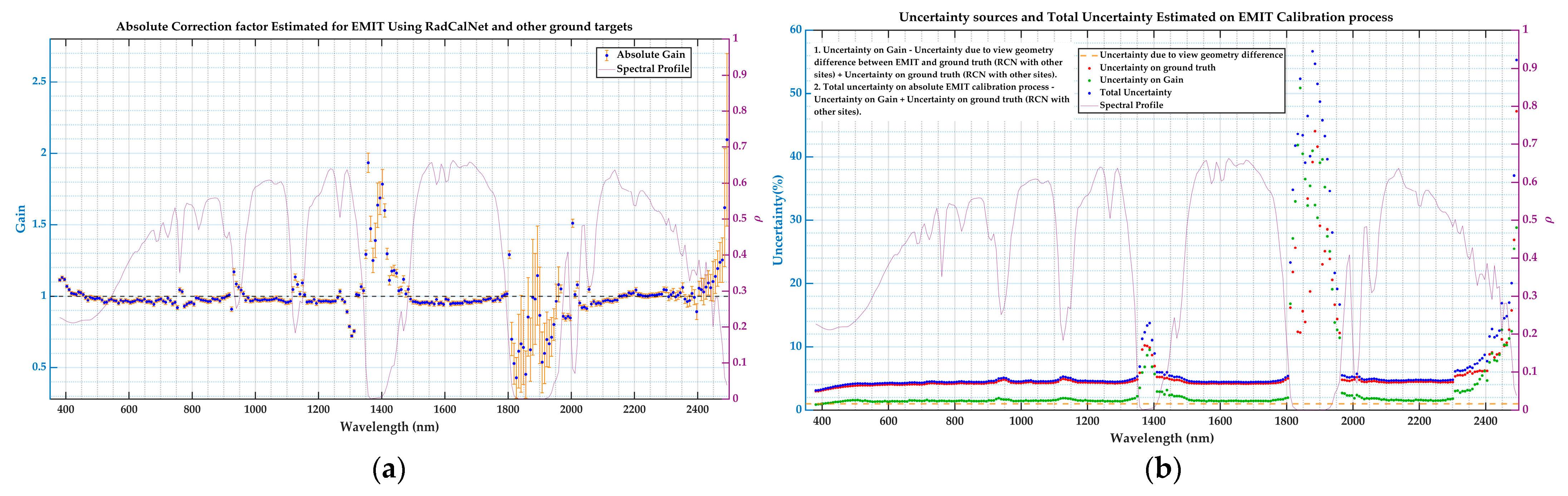
2.2.4. Vicarious Absolute Calibration of EMIT

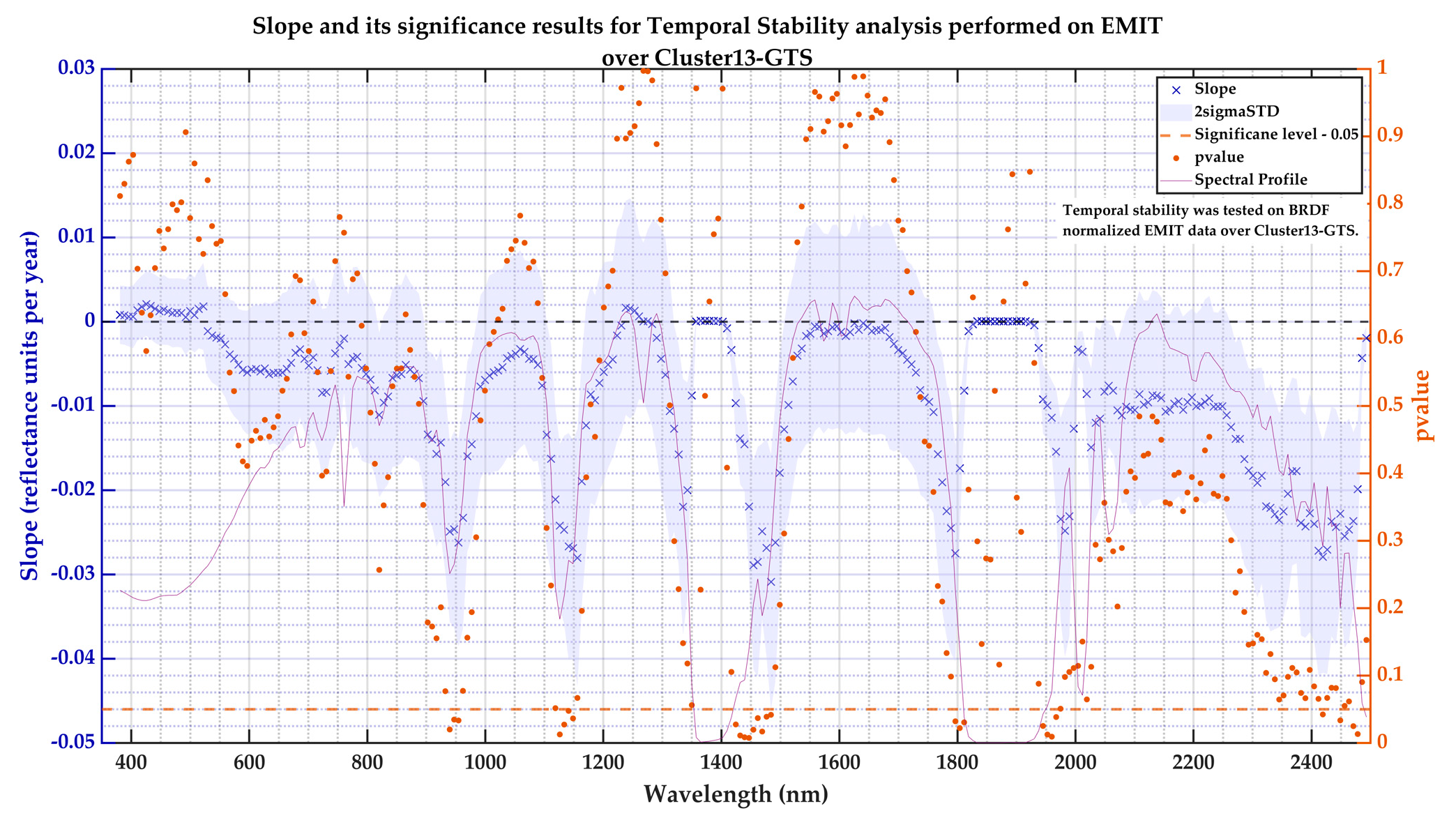
Temporal Stability Evaluation of EMIT

Being on ISS for a year and a half during this work, EMIT had limited temporal coverage compared to DESIS, making it difficult for a temporal stability evaluation. Yet, stability monitoring was performed with the available temporally sparse data. The EMIT images over Cluster13–GTS, comprising 700 data points, were utilized for this process. The data pre–processing, like extracting cloud–free scenes, TOA reflectance, and performing BRDF normalization on that TOA reflectance following Sections Cloud Filtering, TOA Reflectance Computation, and BRDF Normalization, respectively, were initially completed before the evaluation of sensor temporal stability.

The pre–processed data and the uncertainty estimated using Equation (16) were placed on a statistical linearity test for a stability evaluation. The data’s uncertainty was estimated using the same Equation (12) as that used for OLI in the temporal stability of Cluster13–GTS Section 2.2.2. In that equation, all the uncertainty components’ representation remains the same except for $U_{total,EMIT}^2$ replacing $U_{total,OLI}^2,$ and $U_{sensor}^2$ EMIT was considered the 10% sensor absolute accuracy adapted from Green, R.O. et al.’s performance evaluation paper [37], where the author specified the TOA radiance matchup exceeding the 10% requirement.

A Monte Carlo linear regression was performed on the EMIT BRDF–normalized data propagating the uncertainty to perform a temporal stability evaluation of EMIT. The same steps as Cluster13–GTS temporal stability and DESIS linearity were followed for EMIT. The slope and the uncertainty on the slope obtained from the linear fit were tested for statistical significance, as explained in the statistical tests Section Slope Test. Based on the test, EMIT was considered stable over its orbit time.

Given the limitations of the performance and on–orbit calibration papers by Thompson, D.R. et al. and Green, R.O. et al., respectively [36,37], and the inherent uncertainty in the sensor data, it was determined that the absolute calibration of EMIT data was indeed needed. This was to evaluate EMIT’s absolute radiometric accuracy on the TOA reflectance product and to have a better understanding of the uncertainty. Hence, the approach was established to focus on cross–calibrating Hyperion with well–understood uncertainty on the process. The following section briefly explains the steps involved in the absolute calibration process of EMIT.

EMIT Reflectance–Based Absolute Correction Using RCN and In–Situ Measurements

• EMIT Data selection and filtering

Like in DESIS, the same process was followed for EMIT data selection over in –situ targets or ground truths. The main difference between the EMIT and DESIS processes was using other ground truths and RCN due to EMIT’s orbital life span and selective data acquisition. EMIT cloud–free images at the coinciding and near–coinciding dates over RCN sites (RVUS, BSCN, and LCFR), LT, AD, and SDSU were downloaded from NASA’s Earth Data Search, ensuring that the view geometry was <11 degrees. These data were used in the absolute gain estimation. Due to a lack of data from South Africa, the GONA site was unavailable for EMIT. As explained earlier for DESIS, the EMIT view geometry difference was also kept at <11 degrees. Hence, the view geometry difference error was estimated using the same Equation (18), replacing $VZ{A}_{DESIS}$ with $VZ{A}_{EMIT}$ (EMIT’s view zenith). After filtering, 17 data points from all the sites were used to estimate the absolute correction factor. The

Table 3. Showing the number of data points over each site used in the absolute correction factor estimation for EMIT.

Sites	RVUS	BSCN	LCFR	Lake Tahoe (LT)	Algodones Dunes (AD)	SDSU
Dates	7	1	3	3	1	2

below shows the number of coinciding and near–coinciding dates for individual sites. Except for BSCN, all the other sites had coinciding dates.

2.

TOA Reflectance Extraction

• EMIT ROI TOA Reflectance Extraction:

After obtaining the scenes, the cloud–free scenes were used to extract TOA reflectance from the ROI for all sites used in the work. As explained in site overview Section 2.1.2, due to EMIT GSD being 60 m, the ROIs given in the RCN site guide were used [44,45,46] for RVUS and BSCN, but for LCFR, the extended ROI was used. ROI sizes of 1 km × 1 km (~17 pixels × 17 pixels) for the RVUS site, 300 m × 300 m (~5 pixels × 5 pixels) for the BSCN site, 180 m × 180 m (~3 pixels × 3 pixels) for the LCFR site, and 4172 m × 3696 m (~70 pixels × 62 pixels) were used for RCN sites. An ROI of size of 3924 m × 2500 m (~66 pixels × 42 pixels) was used for LT and AD. Finally, for two SDSU vegetative sites, ROIs of sizes of 60 m × 120 m (~1 pixel × 2 pixels of Soybean) and 180 m × 180 m (~3 pixels × 3 pixels of grass) were used. Later, the TOA reflectance from the DNs in the ROI intersecting area of EMIT images was extracted following the TOA computation of EMIT in the Section TOA Reflectance Computation.

• Reference TOA Reflectance Extraction:

For EMIT, extracting TOA reflectance from RCN products was replicated as DESIS. BSCN with the near–coinciding dates, an additional uncertainty estimated due to near coinciding in the DESIS Section DESIS Reflectance–Based Absolute Correction Using RCN was added to the actual uncertainty provided by the RCN following the ISO–GUM technique mentioned in the above sections using the same Equation (19).

Temporal interpolation using linear interpolation was performed following the same technique as DESIS to normalize the acquisition time difference between EMIT and RCN. Finally, after temporal interpolation, RCN data were spectrally interpolated to align with the EMIT spectrum, as EMIT was considered an uncalibrated sensor in this work. Spectral interpolation was also accomplished following the technique used in DESIS Section DESIS Reflectance–Based Absolute Correction Using RCN.

Apart from RCN sites, for other sites, direct TOA reflectance and its uncertainty obtained, as expressed in the site overview section, were subjected to spectral integration to correct for the spectral difference between the ground measurement and EMIT. This spectral–interpolated TOA reflectance of RCN and other sites was used to estimate the absolute gain factor for EMIT.

3.

EMIT Gain Calculation

After TOA reflectance extraction from the sensor, in this case, EMIT and reference, the weighted 1:1 developed for the DESIS calibration was used to estimate the absolute correction factor for EMIT. In contrast to DESIS, the uncertainty on EMIT’s ROI TOA reflectance was attributed to uncertainty only regarding the difference in view geometry, and the uncertainty given in the ground product that is spectrally interpolated was considered uncertainty on the reference TOA reflectance.

The exact weighted 1:1 linear fit through the Monte Carlo approach with 1000 iterations performed for DESIS was also used for EMIT to estimate the absolute correction factor. Random samples were generated based on the primary inputs’ PDFs and propagated through that 1:1 linear regression model. Like DESIS, EMIT bias was assumed to be zero as they have a zero–point estimation or dark current measurement on board [36]. Once again, even here, the mean and standard deviation of the slope values obtained from the Monte Carlo simulation were referred to as the absolute correction factor/gain and the uncertainty on that gain, respectively.

Finally, the gain and its uncertainty can correct the EMIT data to obtain absolute calibrated EMIT by following the equation below.

$${\rho }_{\lambda ,absEMIT}={\rho }_{\lambda ,EMIT}\ast gai{n}_{\lambda },$$

(22)

where ${\rho }_{\lambda ,absEMIT}$ corresponds to absolute corrected EMIT TOA reflectance, ${\rho }_{\lambda ,EMIT}$ represents the original (uncorrected) EMIT TOA reflectance (for this work, BRDF–normalized EMIT TOA reflectance), and gain is the absolute correction factor estimated using Monte Carlo 1:1 linear regression.

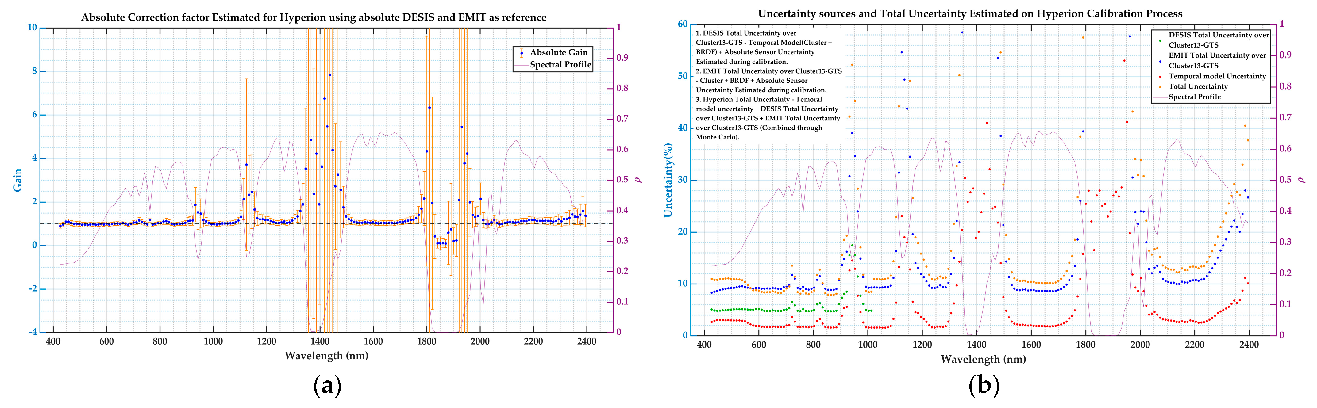
2.2.5. Cross–Calibration of Hyperion Using Absolute DESIS and EMIT

As mentioned, the lifetime absolute calibration research performed by Jing, X. et al. [23] has encountered the need for the temporal de–trending of Hyperion using Libya4. The mentioned Hyperion over Cluster13–GTS was subjected to a temporal stability test to ensure the need for temporal de–trending. Like all other temporal stability evaluations performed in previous sections, cloud–free BRDF–normalized Hyperion TOA reflectance over Cluster13–GTS of about 640 data points, along with its uncertainty, was put under a statistical linearity test. Like all other sensors, the cloud–free BRDF–normalized Hyperion TOA reflectance was obtained following the pre–processing steps. The uncertainty was calculated through ISO–GUM using Equation (12), replacing $U_{total,OLI}^2$ with $U_{total,Hyperion}^2,$ and $U_{sensor}^2$ Hyperion was considered 5%, following McCorkel, J. et al. [38], where the author showed the Hyperion accuracy to be 3–5% over the spectrum, except for deep absorption bands.

Like EMIT’s stability evaluation process, Hyperion was tested through the same Monte Carlo linear regression. Repeating the same process to obtain the slope and uncertainty on the slope from the linear fit and testing the slope for statistical significance, the necessity for the temporal de–trending of Hyperion was confirmed. In fact, there are studies mentioned in the introduction providing enough evidence for temporal drift in Hyperion. This section focuses on improving the temporal de–trending technique for Hyperion and its absolute calibration improvement. The upcoming subsections briefly explain the methodology developed to achieve this goal.

Hyperion Temporal Correction Model Generation

Following the DESIS process to generate a temporal correction model from Section DESIS Temporal Correction Model Generation, a temporal correction model for Hyperion was generated for temporal de–trending. The Hyperion data over Cluster13–GTS listed in the above section were used to achieve this. Through visual inspection, six different models were selected for further statistical analysis to identify the optimal de–trending model. These models, including linear, exponential, logarithmic, poly2, linear–log model, and poly2–log, were tested using statistical methods in R. The model that met the criteria in the earlier Section DESIS Temporal Correction Model Generation was deemed the best de–trending model.

To evaluate the regression models statistically, BRDF–normalized TOA reflectance and a decimal year since the Hyperion launch were used as dependent and independent variables, respectively. Again, weights were included to propagate uncertainty in the model generation. These weights were calculated as the inverse square of the estimated uncertainty in BRDF–normalized TOA reflectance. This uncertainty was calculated using the same Equation (15) used for DESIS.

The R results were obtained for all Hyperion hyperspectral bands using the abovementioned inputs. To summarize the results, the steps used for DESIS were replicated: Hyperion data were converted to OLI bands using Equation (10) from the spectral integration Section Normalization of Spectral Difference, and regression analysis was performed using the multispectral Hyperion data in R. Like DESIS, although different models are observed to have higher F–scores, based on the associated p–values, RSE, and visual inspection, the poly2 model was indicated as a statistically significant fit to the underlying data. Similar results were seen for hyperspectral bands. Therefore, the poly2 model was adopted for the temporal de–trending of Hyperion data. Even for Hyperion, the uncertainty in the temporal correction model was considered to be the RMSE, representing the model error like in DESIS.

Following Equation (23) provides the temporal de–trended data for Hyperion.

$${\rho }_{\lambda ,\mathrm{p}\mathrm{r}\mathrm{e}\mathrm{d}\mathrm{i}\mathrm{c}\mathrm{t}\mathrm{e}\mathrm{d}}={\beta }_0+{\beta }_{1}X+{\beta }_2{X}^2,$$

(23)

$${\rho }_{\lambda ,tempHyperion}={\displaystyle \frac{{\rho }_{\lambda ,reference}}{{\rho }_{\lambda ,predicted}}}\times {\rho }_{\lambda ,BRDF NormalizedHyperion},$$

(24)

where ${\beta }_0-{\beta }_2$ are the coefficients of the poly2 model, whereas ${\rho }_{\lambda ,\mathrm{p}\mathrm{r}\mathrm{e}\mathrm{d}\mathrm{i}\mathrm{c}\mathrm{t}\mathrm{e}\mathrm{d}}$ is the TOA reflectance predicted by the model, with X being the decimal year since launch, ${\rho }_{\lambda ,reference}$ is the TOA reflectance predicted at the Hyperion launch year (X = 0), and ${\rho }_{\lambda ,BRDF NormalizedHyperion}$ corresponds to the BRDF–normalized Hyperion data, and finally, ${\rho }_{\lambda ,tempHyperion}$ represents the temporal de–trended Hyperion data.

Hyperion Absolute Correction Factor Estimation Using DESIS and EMIT

To estimate the absolute correction factor to keep hyperspectral sensors on absolute radiometric consistency or, in other words, to achieve the goal of integrating/combining all hyperspectral sensors interchangeably, absolute calibrated DESIS and EMIT were used. The BRDF–normalized, temporal de–trended, absolute corrected DESIS (${\rho }_{\lambda ,absDESIS}$) and BRDF–normalized, absolute corrected EMIT (${\rho }_{\lambda ,absEMIT}$) over Cluster13–GTS with their respective total uncertainties obtained from equations under total uncertainty, Section DESIS and EMIT, were spectrally integrated to match the Hyperion spectrum. This spectral integration was performed following Equation (10) from the spectral integration in Section Normalization of Spectral Difference and used as one reference dataset (${\rho }_{\lambda ,absref}$) with 2343 data points (1643 DESIS and 700 EMIT).

Due to the lack of temporal overlap between Hyperion and DESIS, EMIT (because of differences in the operational time frames) has no coinciding dates for performing 1:1 regression. Given this limitation of overlapping time but the knowledge of the fact that the Cluster13–GTS site provides known levels of stability over extended periods, a different approach was taken to estimate the calibration factor for Hyperion. Random sampling through a Monte Carlo simulation was used to calculate the gain. The process followed is shown in the flowchart Figure 8 below. The first 1000 random samples for each Hyperion band were generated based on the primary inputs’ PDFs where the reference dataset (${\rho }_{\lambda ,absref}$) and BRDF–normalized, temporal de–trended Hyperion (${\rho }_{\lambda ,tempHyperion}$), along with their respective uncertainties, are considered inputs. The results of these random samples were sized as 1000 × 2343 for the reference and 1000 × 640 for Hyperion.

This approach considers randomly selecting n data from the reference and Hyperion random samples and taking the ratio of the reference over Hyperion n times using Equation (25) below. This process is repeated for 1000 iterations for each Hyperion band, ensuring no repetition of the same sample while randomly selecting the data. Here, n was taken as 500, as the random selection size should be less than the size of inputs. Hence, 1000 × 500 ratios are obtained for each band.

$$Rati{o}_{\lambda }={\displaystyle \frac{{\rho }_{\lambda ,absref}}{{\rho }_{\lambda ,tempHyperion}}},$$

(25)

Later, the mean and standard deviation of 500 ratios were calculated, resulting in 1000 ratios and standard deviations for each band. Finally, the mean of the 1000 ratios was calculated, which was considered the gain or correction factor, and the mean of the 1000 standard deviations was considered as the uncertainty on the gain. This was performed on a per–band basis, resulting in a calibration factor on each band along with uncertainty. The uncertainty estimated on the gain was considered incorporating both DESIS and EMIT uncertainty along with Hyperion temporal de–trending model uncertainty, hence making this uncertainty the total uncertainty on the Hyperion cross–calibration technique.

$${\rho }_{\lambda ,absHyperion}={\rho }_{\lambda ,tempHyperion}\ast gai{n}_{\lambda },$$

(26)

The application of the gain obtained was made using the Equation (26) similar to that of DESIS, where ${\rho }_{\lambda ,absDESIS}$ is replaced with ${\rho }_{\lambda ,absHyperion}$ and ${\rho }_{\lambda ,tempDESIS}$ with ${\rho }_{\lambda ,tempHyperion}$.

Hyperion Statistical Test for Linearity Check After Temporal De–Trending

The gain estimated in the previous section was later applied to the BRDF–normalized, temporal de–trended Hyperion data (${\rho }_{\lambda ,tempHyperion}$) over Cluster13–GTS to obtain the BRDF–normalized, temporal de–trended, absolute corrected Hyperion data (${\rho }_{\lambda ,absHyperion}$) using the same Equation (21) as for DESIS, replacing appropriate terms, which is Equation (26). Then, like all the stability assessments, a statistical test was performed to validate the temporal correction, following the process described in the temporal stability evaluation Section 2.2.2, a Monte Carlo linear regression that absolute corrected Hyperion data propagating the total uncertainty. The slope and the uncertainty of the slope obtained from the linear fit were then tested for statistical significance, which was covered under the statistical tests Section Slope Test, like all others.

2.2.6. Validation of Calibration Coefficients

Validating the calibration techniques is crucial to ensure the reliability and accuracy of the developed methodology. This study validated the calibration techniques using OLI and a combination of OLI and ETM+ generated in Section 2.2.2 as a validation reference. The choice of the validation reference was based on the hyperspectral sensor’s temporal coverage; for instance, DESIS and EMIT used OLI from 2019 to 2024 and 2022 to 2024, respectively. The following section discusses the validation process.

Validation of DESIS, EMIT, and Hyperion Calibration Coefficients

To validate the hyperspectral sensors’ (DESIS, EMIT, or Hyperion) calibration technique developed (in their respective Section 2.2.3, Section 2.2.4 or Section 2.2.5), the absolute corrected sensor (${\rho }_{\lambda ,absDESIS}$ or ${\rho }_{\lambda ,absEMIT}$ or ${\rho }_{\lambda ,absHyperion}$) data and their total uncertainty were spectrally integrated using Equation (10) from the Section Normalization of Spectral Difference to ensure that it was spectrally consistent with OLI prior to validation. Multispectral simulated data were then tested for statistical similarity with absolute OLI data. To check for similarities between the two means, Welch’s t–test was performed following the description under the Statistical Tests Section Welch’s t–Test or Mean Test. The validation was performed on a per–sensor basis, meaning that the similarity test for validation was performed on each hyperspectral sensor with OLI individually. OLI is considered the validation reference, assuming that it is well–calibrated.

Comparison of Old and New Calibration Techniques for Hyperion

To compare the calibration performed on Hyperion by Jing, X. et al. [23] with the new calibration, both were applied on Cluster13–GTS and Libya4 cloud filtered and BRDF–normalized TOA reflectance. First, the temporal de–trending and absolute correction developed in the paper (version2) were applied for both sites using Equations (24) and (26), respectively. Then, the following Equations (27)–(29) [23] applied the drift correction and gain application from the old calibration (version1) to the sites.

$${\displaystyle \frac{{\%drift}_{\lambda }}{year}}={\displaystyle \frac{slop{e}_{\lambda }\ast 365\ast 100}{intercep{t}_{\lambda }}},$$

(27)

$${\rho }_{\lambda ,driftHyperion}={\rho }_{\lambda ,Hyperion}-{\displaystyle \frac{\frac{{\%drift}_{\lambda }}{year}\ast DY}{100}},$$

(28)

$${\rho }_{\lambda ,absHyperion}={\rho }_{\lambda ,driftHyperion}\ast gai{n}_{\lambda }+bia{s}_{\lambda },$$

(29)

where ${\%drift}_{\lambda }$ per year is the per–year–per–band degradation (%) obtained through the coefficients (slope and intercepts) of linear regression on the per–band TOA reflectance, ${\rho }_{\lambda ,driftHyperion}$ is the drift–corrected Hyperion TOA reflectance, ${\rho }_{\lambda ,Hyperion}$ is the BRDF–normalized TOA reflectance, and DY is the decimal year. Lastly, the ${\rho }_{\lambda ,absHyperion}$ absolute corrected Hyperion TOA reflectance was achieved after applying the calibration coefficients gain and bias for each spectral band.

Finally, the absolute corrected Hyperion TOA reflectance from both calibration techniques was subjected to Monte Carlo linear regression considering the total uncertainty. For the new technique, the total uncertainty was obtained from the Hyperion calibration section of this paper, and for the old technique, the total uncertainty was calculated using the same Equation (12) used for OLI with the absolute radiometric uncertainty on the sensor to be 5%. The slope and its uncertainty obtained were subjected to a significance test following the Section Slope Test, and the mean absolute TOA reflectance obtained from both the calibration versions were tested for statistical similarity using the Section Slope Test.

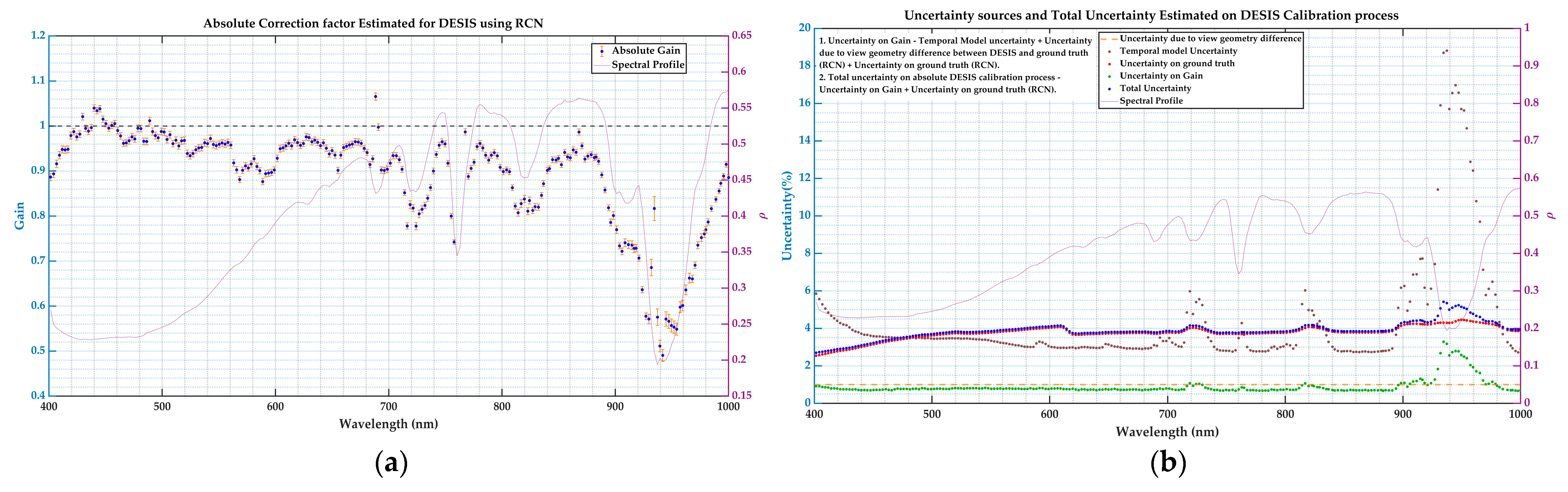
2.2.7. Uncertainty Analysis

In each process step, uncertainties from previous steps are propagated to the next step. The equations used to estimate the uncertainties are mentioned in their respective sections, but this section mainly discusses the uncertainty flow towards obtaining the total uncertainty for the process.

DESIS and EMIT

For DESIS and EMIT, the absolute calibration process was performed following the same technique, making the uncertainty propagation similar, except the temporal de–trending step was not performed on EMIT. DESIS was temporally de–trended before calibration, for which the temporal model was generated propagating the Cluster13–GTS uncertainty combined with BRDF model uncertainty through ISO–GUM using Equation (15). Due to this, before the calibration coefficient estimation for DESIS, the DESIS TOA reflectance over ground targets was subjected to temporal de–trending. This introduces the need to combine temporal model uncertainty with uncertainty to view the geometry difference using Equation (20).

$$U_{total,Sensor}^2=\sqrt{U_{Gain}^2+{U\prime }_{RCN}^2},$$

(30)

Equation (30) was used to estimate the total uncertainty on calibration $U_{total,Sensor}^2$ for both DESIS and EMIT by combining uncertainty on the absolute gain obtained and uncertainty provided by the ground truth, where RCN is for DESIS and other sites along with EMIT. The entire uncertainty flow for both sensors is shown in Figure 9 below. To use the absolute calibrated DESIS and EMIT for Hyperion cross–calibration over the Cluster13–GTS site, the total uncertainty over Cluster13–GTS data for both DESIS and EMIT was estimated using the equations below.

$$U_{Cluster13-GTS,DESIS}^2=\sqrt{U_{total,Sensor}^2+U_{Temporal model}^2},$$

(31)

where $U_{Cluster13-GTS,DESIS}^2$ represents the total uncertainty on DESIS over Cluster13–GTS, $U_{total,Sensor}^2$ represents the total calibration uncertainty, and finally, $U_{Temporal model}^2$ represents the uncertainty on the temporal model, which incorporates the Cluster13–GTS uncertainties and BRDF model uncertainty.

$$U_{Cluster13-GTS,EMIT}^2=\sqrt{U_{total,Sensor}^2+U_{Cluster}^2+U_{BRDF}^2},$$

(32)

Like DESIS $U_{Cluster13-GTS,EMIT}^2$ represents the total uncertainty on EMIT over Cluster13–GTS, $U_{total,Sensor}^2$ represents the total calibration uncertainty, and as there is no temporal de–trending for EMIT, the uncertainty on the temporal model is replaced with the Cluster13–GTS uncertainties $U_{Cluster}^2$ and BRDF model uncertainty $U_{BRDF}^2$ in it.

Hyperion

Unlike DESIS and EMIT for the absolute calibration of Hyperion, absolute DESIS and EMIT over Cluster13–GTS, along with the total uncertainty estimated from Equation (31), were the reference. As mentioned in earlier sections, the Hyperion data over Cluster13–GTS were subjected to temporal de–trending. Finally, the temporal model uncertainty for Hyperion and absolute DESIS and EMIT uncertainties were propagated to the absolute cross–calibration gain estimation. The following flowchart Figure 10 shows the flow of uncertainty.

2.2.8. Statistical Tests

The stability monitoring of the target and the sensors was a critical step in this work, followed by the quantification required to validate the calibration coefficient estimated for all three hyperspectral sensors. Two statistical tests were implemented to validate the temporal de–trending and calibration performed in the work. The subsections below briefly explain the tests performed.

Slope Test

The significance of the linear regression coefficient (slope) can be performed to monitor the stability of the target or sensor by itself. The slope with its uncertainty obtained from the linear fit is tested for statistical significance using a two–tailed, one–sample t–test [61]. The hypothesis is that the slope on the regression line equals zero (null hypothesis). The t–statistics follow a t–distribution with a degree of freedom, df = n − 2 (n: number of observations), and are obtained by Equation (33).

Null hypothesis: H₀: β₀ = 0

Alternative hypothesis: H_A: β₀ ≠ 0

$$t={\displaystyle \frac{\beta 0}{Sb}},$$

(33)

where β₀ corresponds to the regression coefficient (slope) and S_b corresponds to the standard error on the slope. The p–value corresponding to the t–score indicates the significance of the slope. If the p–value is less than the significance level (0.05), it implies that there is insignificant evidence to reject the null hypothesis, meaning the slope is statistically indifferent to zero.

Welch’s t–Test or Mean Test

A statistical test called Welch’s t–test was applied to evaluate if the calibrated TOA reflectance of the hyperspectral sensors DESIS, EMIT, and Hyperion is statistically equivalent to that of Landsat TOA reflectance. Welch’s test [63] helps to validate the calibration technique by comparing two means. This test compares the difference between the means, considering their respective uncertainties and assessing whether the difference is statistically significant. Here, the variances calculated as uncertainty squares are unequal for all the sensors due to different uncertainties on each sensor. The hypothesis for Welch’s test, along with its t–test, was performed using Equation (34).

Null hypothesis: H₀: ${\rho }_{\lambda ,OLI}$ = ${\rho }_{\lambda ,absSensor}$

Alternative hypothesis: H_A: ${\rho }_{\lambda ,OLI}$ ≠ ${\rho }_{\lambda ,absSensor}$

$$t={\displaystyle \frac{{\rho }_{\lambda ,OLI}-{\rho }_{\lambda ,absSensor}}{\sqrt{U_{total,OLI}^2+U_{total,Sensor}^2}}},$$

(34)

where ${\rho }_{\lambda ,OLI}$ corresponds to the BRDF–normalized OLI TOA reflectance and ${\rho }_{\lambda ,absSensor}$ corresponds to the absolute corrected spectral integrated hyperspectral sensor TOA reflectance with their respective total uncertainties $U_{total,OLI}^2$ and $U_{total,Sensor}^2$, respectively. Here, the null hypothesis assumes that the two given means are equal. The p–value corresponding to the t–score indicates the significance of the difference. Suppose the p–value is greater than the significance level (0.05). In that case, it implies that the difference between two populations is likely due to random possibilities, meaning there is not enough evidence to reject the null hypothesis.

3. Results and Analysis

The Results and Analysis section presents the outcomes of the cross–calibration methodology developed for Hyperion. It details the results of temporal stability and radiometric accuracy assessments conducted on all three hyperspectral sensors used in this study, including the necessary corrections performed. The section initially presents the analysis of the temporal stability of the Cluster13–GTS used for calibration. Finally, it validates the correction factors derived.

3.1. Data Processing

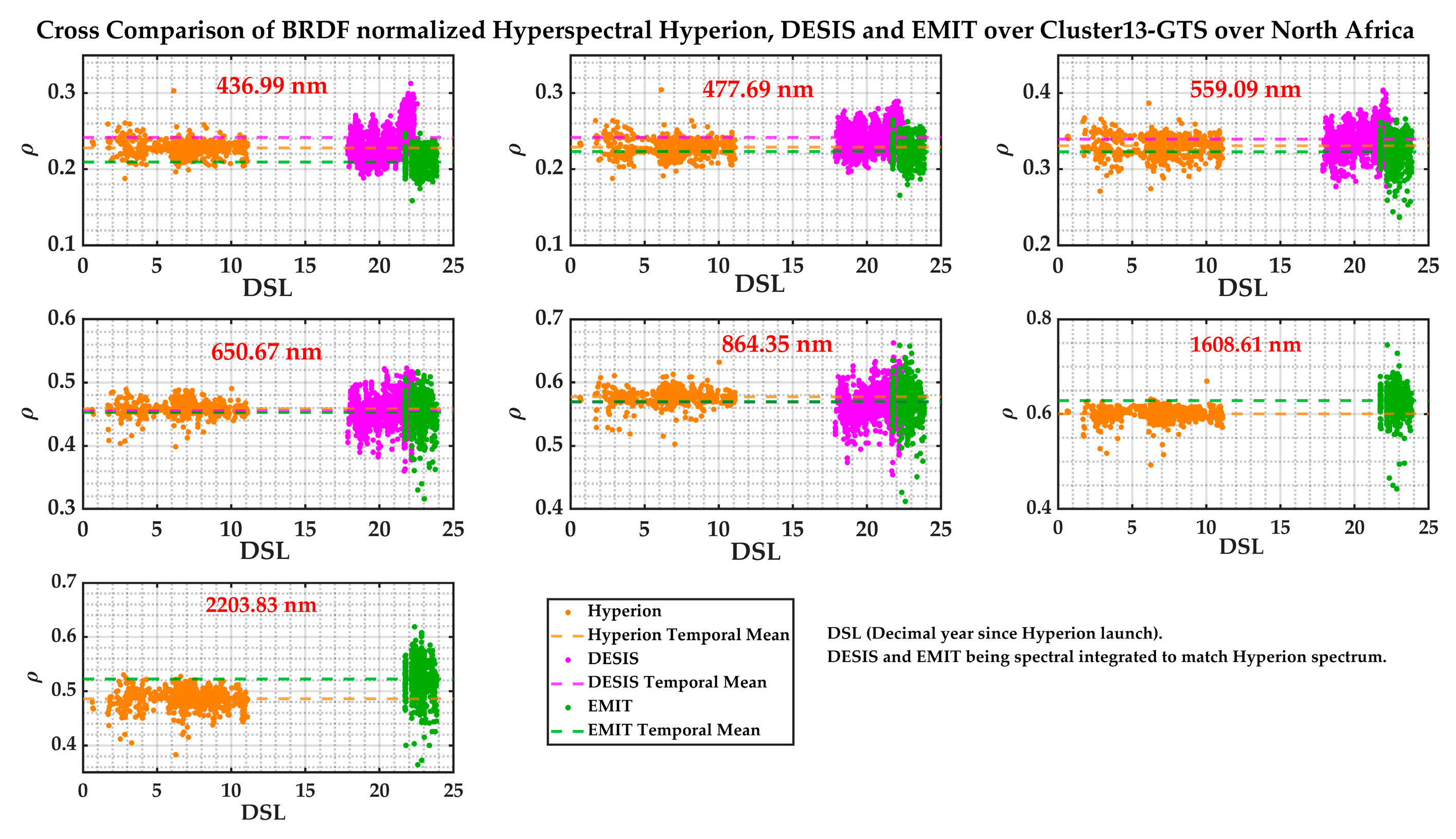
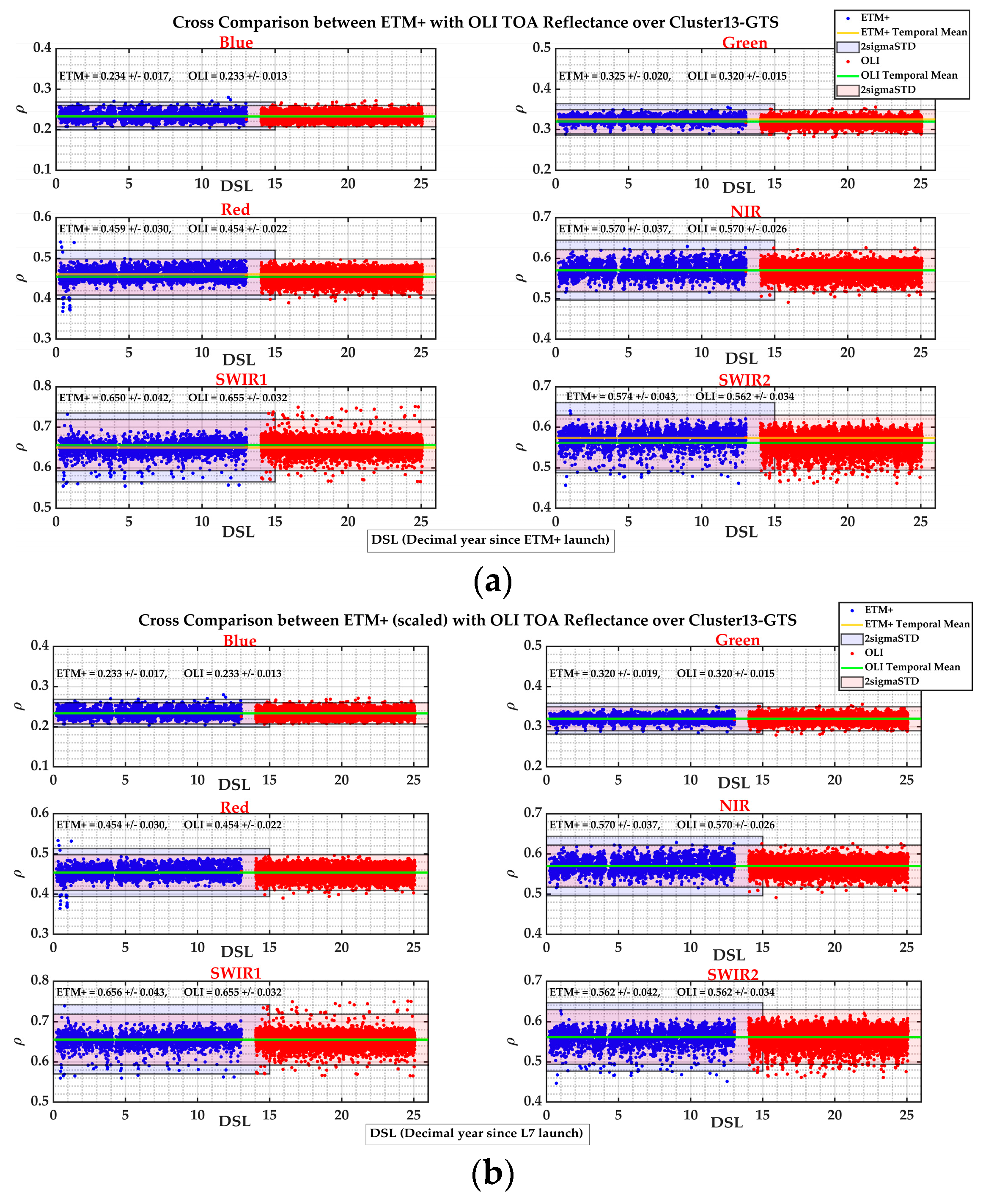
BRDF Normalization

BRDF normalization performed on all the sensors (used in this work) cloud–filtered data over Cluster13–GTS in the methodology Section BRDF Normalization was used to normalize the seasonal effect (shown in Figure 6a) due to solar angular geometry difference. Additionally, it accounted for the difference in the view geometry for sensors on ISS, which are DESIS and EMIT. Figure 11 shows the example of OLI TOA reflectance over Cluster13–GTS before and after BRDF normalization. This example demonstrates the effectiveness of the 4–angle BRDF model in successfully normalizing (using Equation (7)) the seasonal effect. The example illustrates the improvement in the Cluster13–GTS directional effect after applying the model. This is more prominently seen on the longer wavelengths, like SWIR1 and SWIR2, as the angular effect is pronounced as we move to longer spectrum wavelengths. For example, in the SWIR1 channel of the figure, the pre–normalized data (blue) exhibit a sinusoidal (or oscillatory) pattern, indicating the variation in solar positions for different seasons over a year. This pattern was substantially reduced by applying the BRDF model (orange data seen in the figure).

This BRDF normalization was crucial to ensure that the data used for cross–calibration and the other processes involved in the study were not influenced by the sensors’ varying angular geometries (view and illumination). A more direct comparison was possible by removing the seasonal (or BRDF) effect and those angular variations.

3.2. Temporal Stability Evaluation of Cluster13–GTS Since 1999 Results

As discussed, the assessment of Cluster13–GTS temporal stability since 1999 focused on discounting potential site–related trends. This was essential in the study’s sensor stability monitoring and enabling accurate cross–calibration. The analysis involved cross–comparing ETM+ and OLI, leveraging the assumption of OLI’s established calibration accuracy. To account for the spectral difference between the sensors, the BRDF–normalized ETM+ reflectance data over Cluster13–GTS were adjusted using SBAFs (

Table 4. SBAFs and scaling factors applied to ETM+ bands to match OLI spectral characteristics and absolute values, respectively.

Band	Blue	Green	Red	NIR	SWIR1	SWIR2
SBAF	1.0025	0.9977	0.9915	1.0832	1.0083	1.0657
Scaling Factor	0.9983	0.9830	0.9876	0.9990	1.0097	0.9792

), which was estimated through Monte Carlo using the hyperspectral profile of Cluster13–GTS, thus ensuring the consistency between ETM+ and OLI data. Figure 12a presents the cross–comparison between BRDF–normalized, SBAF–corrected ETM+ (blue), and BRDF–normalized OLI (red) TOA reflectance over Cluster13–GTS with their respective total uncertainties (shaded area).

The figure demonstrates strong agreement between the mean TOA reflectance of both sensors across all the bands. While both datasets (blue and red) exhibit some compactness at shorter wavelengths, a slight increase in noise (variability seen in the datasets) is observed in the longer wavelength (SWIR) channels. This is likely attributable to lower signal levels in these spectral regions. ETM+ exhibited uncertainties of 6–7.5%, while OLI data showed uncertainties of 4.5–6%, based on the EPICS with an uncertainty of 3–4%.

Table 5. Uncertainty sources and total uncertainty percentages for all Landsat sensors for their respective bands.

Uncertainty Sources (%)	Sensor	CA	Blue	Green	Red	NIR	SWIR1	SWIR2
Cluster Uncertainty	ETM+	–	4.7159	2.8821	3.7549	3.5434	3.6418	4.8787
	OLI	4.2456	4.2348	3.1057	3.3724	2.9888	3.2714	4.4229
BRDF	ETM+	–	2.6950	1.5944	1.9861	1.7830	1.8928	2.7666
	OLI	2.2604	2.2949	1.7633	1.8990	1.7958	1.8948	2.7576
Sensor’s Uncertainty	ETM+	–	5	5	5	5	5	5
	OLI	3	3	3	3	3	3	3
SBAF	ETM+	–	0.4958	0.5115	0.6782	1.0822	0.9482	0.6462
Total Uncertainty	ETM+	–	7.3992	6.0092	6.5957	6.4735	6.5379	7.5414
	OLI	5.6687	5.6745	4.6642	4.8969	4.5997	4.8262	6.0138

details the total uncertainty and its contributing sources for each sensor. Although minor shifts in the mean TOA reflectance are noticeable in some bands, the discrepancies remain within the calculated uncertainty bounds. The absence of any temporal trend in the OLI (red) data supports the assumption of its calibration accuracy and stability. The EMT+ (blue) data, consistent with OLI’s uncertainty, further strengthen the agreement between the two datasets. Assuming the temporal stability of both sensors, these results strongly suggest that Cluster13–GTS has maintained temporal stability over the analyzed period.

The visual assessment in Figure 12a was further quantified through linear regression analysis followed by a statistical significance test on the resulting slope.

Table 6. Slope values, with the 1σ uncertainty (standard deviation), and the p–values from applying a slope significance test for the temporal stability analysis of Cluster13–GTS.

Time Frame (Sensor)		CA	Blue	Green	Red	NIR	SWIR1	SWIR2
1999–2012 (ETM+)	Slope +/− std	–	−9.09 × 10−5 +/− 1.65 × 10−4	−3.34 × 10−5 +/− 1.93 × 10−4	3.30 × 10−4 +/− 2.94 × 10−4	4.31 × 10−4 +/− 3.52 × 10−4	6.18 × 10−4 +/− 4.06 × 10−4	7.29 × 10−4 +/− 4.28 × 10−4
	p–value	–	0.5825	0.8629	0.2622	0.2207	0.1276	0.0885
2013–2024 (OLI)	Slope +/− std	1.17 × 10−5 +/− 8.46 × 10−5	−5.74 × 10−6 +/− 8.97 × 10−5	−1.10 × 10−4 +/− 9.92 × 10−5	−5.39 × 10−5 +/− 1.48 × 10−4	−1.12 × 10−4 +/− 1.77 × 10−4	−2.32 × 10−4 +/− 2.14 × 10−4	−1.44 × 10−4 +/− 2.28 × 10−4
	p–value	0.8898	0.9490	0.2680	0.7167	0.5253	0.2803	0.5270

presents the calculated slopes with their associated 1σ uncertainties and the p–values obtained from the significance test. The result reveals small, statistically non–significant slopes across all the bands for both time frames. In every case, the magnitude of the slope is smaller than its associated standard deviation, indicating that the observed temporal trends are minimal and do not represent a significant change over time. This conclusion is further supported by the p–values, which are all greater than the significance level of 0.05 for both the 1999–2012 and 2013–2024 periods, confirming the temporal stability of the Cluster13–GTS during these intervals. Given the short interval between 2012 and 2013 and the assumption of no significant changes to Cluster13–GTS during this gap, the site can be considered temporally stable from 1999 to 2024.

To prepare the ETM+ (1999–2012) and OLI (2013–2024) datasets for subsequent calibration validation, the ETM+ data were scaled to match the OLI data. This involved applying the scaling factors in Table 4 with the previously determined SBAF values. Figure 12b illustrates the results of this scaling process applied to the ETM+ dataset. This harmonized dataset was then utilized to validate all hyperspectral sensor calibrations.

3.3. Vicarious Absolute Calibration of DESIS Results

3.3.1. DESIS Temporal Correction Model Generation

Having established the temporal stability of the Cluster13–GTS, the observed trend in DESIS during the cross–comparison with other hyperspectral sensors (Hyperion and EMIT) cloud–screened, BRDF–normalized mean TOA reflectance data over Cluster13–GTS (Figure 1) strongly suggests a sensor–related issue. This observation aligns with similar challenges reported by Carmona, E. et al. [35]. To address this, a temporal correction model was developed. Model selection was performed using a statistical approach.

Table 7. Statistical results obtained for all the models that were tested through R to select the best model for the temporal correction of DESIS over its entire lifetime, shown for multispectral bands as a summary.

Criteria	Models	CA	Blue	Green	Red	NIR
Residual Standard Error	Linear	0.2967	0.3306	0.3281	0.3485	0.3474
	Exponential	1.349	1.355	0.9443	0.7366	0.6028
	poly2	0.275	0.3282	0.3282	0.3481	0.3474
	poly4	0.2745	0.3282	0.3274	0.3475	0.3452
F–statistics	Linear	640.8	170.3	99.94	38.03	61.6
	Exponential	629.8	171.6	98.77	35.79	58.01
	poly2	505.8	98.71	50.3	21.53	31.28
	poly4	255.8	49.81	27.6	12.54	21.52
p–value for F–statistics	Linear	2.20 × 10−16	2.20 × 10−16	2.20 × 10−16	8.77 × 10−10	7.58 × 10−15
	Exponential	2.20 × 10−16	2.20 × 10−16	2.20 × 10−16	2.70 × 10−9	4.42 × 10−14
	poly2	2.20 × 10−16	2.20 × 10−16	2.20 × 10−16	5.91 × 10−10	4.69 × 10−14
	poly4	<2.2 × 10−16	<2.2 × 10−16	<2.2 × 10−16	4.79 × 10−10	<2.2 × 10−16
Significance of coefficients	Linear	Constant	Constant	Constant	All	All
	Exponential	Constant	Constant	All	All	All
	poly2	All	All	Constant, 1st order term	Constant, 2nd order term	Constant term
	poly4	All	All	All	Constant, 1st term	All

presents an example of the results of this approach applied to multispectral DESIS Cluster13–GTS data. The first criterion, RSE, appears to be higher than typical due to the inclusion of weights in its calculation. Despite this, the poly4 model exhibits the lowest RSE, indicating a statistically better fit. While the differences in RSE between models are relatively small (excluding the exponential model), the poly4 model also demonstrated significantly lower p–values for F–statistics. As previously mentioned, a p–value below the significance level 0.05 suggests that the overall model adequately represents underlying data, meaning that all the predictor variables contribute significantly to predicting the output.

This observation is further supported by the significance of nearly all the coefficients in the poly4 model (Table 7), with the red band being the sole exception. These findings were reinforced by the analysis results at the hyperspectral scale (Figure 13). The exponential model’s RSE was excluded from Figure 13a due to its substantially higher value. Figure 13a (left) clearly shows the poly4 model’s RSE as the lowest across all the bands, including absorption bands. This is mirrored in Figure 13b (right bottom), where all the p–values, including those for absorption bands, are below the significance level. Though the poly2 model’s performance is comparable to poly4, both RSE and p–values at the multispectral scale indicate that poly4 provides a better fit. Not to depend solely on the statistics for the results, even visually, poly4 was seen to represent the underlying data better than the rest. Therefore, it was concluded that the poly4 model is statistically the most suitable model across the DESIS spectral range for the temporal correction.

Finally, based on the poly4 fit, the temporal correction model was applied to the Cluster13–GTS BRDF–normalized data (blue in Figure 14), effectively correcting the observed temporal trend. As shown in Figure 14, the corrected Cluster13–GTS data (orange) demonstrate the model’s success in mitigating the trend. This correction is significant given the challenges highlighted by Carmona, E. et al. [35] in 2021, who noted the instability and degradation of the sensor’s channels below 450 nm, with reported degradation rates of up to ~20% per year. The inclusion of an additional 2.5 years of data in this analysis revealed trends in some bands above 450 nm as well. Applying this temporal correction addresses a key factor that could otherwise hinder the calibration accuracy, ensuring the reliability of DESIS data for the subsequent analysis. Figure 14 illustrates the temporal trend and its correction in the shorter wavelengths, demonstrating the model’s minimal impact on other bands. The coefficients for this temporal correction model are provided in

Table A1. Showing the temporal correction coefficients (temporal coefficients), absolute correction coefficients (absolute gain), and the total uncertainty estimated on the DESIS absolute calibration process (total uncertainty) for 235 bands.

Wavelengths	Temporal Coefficients					Absolute Gain	Total Uncertainty (%)
	${\mathsf{\beta }}_{\mathbf{0}}$	${\mathsf{\beta }}_{\mathbf{1}}$	${\mathsf{\beta }}_{\mathbf{2}}$	${\mathsf{\beta }}_{\mathbf{3}}$	${\mathsf{\beta }}_{\mathbf{4}}$
401.53	0.2995	−0.0104	−0.0266	0.0115	−0.0009	0.8866	2.70
404.20	0.2751	0.0057	−0.0377	0.0145	−0.0013	0.8937	2.74
406.82	0.2632	0.0082	−0.0337	0.0128	−0.0011	0.9161	2.76
409.33	0.2551	0.0098	−0.0316	0.0118	−0.0010	0.9352	2.78
411.81	0.2491	0.0125	−0.0320	0.0118	−0.0010	0.9479	2.81
414.34	0.2470	0.0137	−0.0314	0.0115	−0.0010	0.9469	2.83
416.91	0.2443	0.0193	−0.0338	0.0120	−0.0011	0.9483	2.86
419.44	0.2353	0.0222	−0.0334	0.0116	−0.0010	0.9789	2.89
422.01	0.2317	0.0231	−0.0325	0.0112	−0.0010	0.9874	2.91
424.64	0.2334	0.0213	−0.0300	0.0103	−0.0009	0.9759	2.93
427.29	0.2304	0.0124	−0.0219	0.0078	−0.0007	0.9819	2.95
429.86	0.2223	0.0239	−0.0290	0.0099	−0.0009	1.0209	2.97
432.45	0.2285	0.0224	−0.0262	0.0091	−0.0009	0.9948	3.00
434.98	0.2293	0.0193	−0.0237	0.0082	−0.0008	0.9887	3.04
437.49	0.2271	0.0185	−0.0226	0.0078	−0.0007	0.9964	3.06
439.95	0.2187	0.0245	−0.0255	0.0085	−0.0008	1.0397	3.10
442.49	0.2199	0.0174	−0.0200	0.0069	−0.0007	1.0341	3.13
445.02	0.2196	0.0118	−0.0154	0.0057	−0.0006	1.0383	3.16
447.76	0.2250	0.0170	−0.0192	0.0067	−0.0007	1.0153	3.19
450.34	0.2273	0.0106	−0.0143	0.0053	−0.0005	1.0052	3.23
452.89	0.2305	0.0056	−0.0105	0.0043	−0.0005	0.9952	3.27
455.57	0.2292	0.0048	−0.0094	0.0039	−0.0004	1.0014	3.31
458.18	0.2286	−0.0002	−0.0055	0.0028	−0.0003	1.0054	3.34
460.75	0.2324	0.0025	−0.0074	0.0033	−0.0004	0.9900	3.38
463.28	0.2351	−0.0011	−0.0044	0.0024	−0.0003	0.9780	3.39
465.82	0.2393	0.0008	−0.0052	0.0026	−0.0003	0.9615	3.42
468.30	0.2392	0.0024	−0.0055	0.0025	−0.0003	0.9625	3.45
470.77	0.2383	0.0033	−0.0054	0.0024	−0.0003	0.9674	3.48
473.36	0.2357	0.0032	−0.0058	0.0025	−0.0003	0.9761	3.50
475.87	0.2368	0.0009	−0.0046	0.0022	−0.0002	0.9713	3.52
478.57	0.2315	0.0002	−0.0034	0.0018	−0.0002	0.9950	3.55
481.24	0.2328	0.0012	−0.0037	0.0018	−0.0002	0.9943	3.57
483.80	0.2408	−0.0057	0.0013	0.0003	−0.0001	0.9660	3.60
486.39	0.2447	−0.0075	0.0044	−0.0005	0.0000	0.9656	3.62
488.99	0.2345	0.0037	−0.0027	0.0011	−0.0001	1.0117	3.64
491.55	0.2417	0.0039	−0.0032	0.0013	−0.0001	0.9876	3.67
493.97	0.2455	0.0057	−0.0041	0.0015	−0.0002	0.9788	3.67
496.50	0.2480	0.0005	−0.0005	0.0005	−0.0001	0.9739	3.68
499.24	0.2464	−0.0040	0.0029	−0.0005	0.0000	0.9878	3.70
501.75	0.2485	−0.0029	0.0015	0.0000	0.0000	0.9867	3.71
504.32	0.2544	−0.0052	0.0024	−0.0002	0.0000	0.9701	3.73
506.92	0.2536	−0.0079	0.0047	−0.0009	0.0001	0.9807	3.75
509.54	0.2616	−0.0064	0.0050	−0.0011	0.0001	0.9608	3.77
512.15	0.2623	−0.0084	0.0071	−0.0018	0.0002	0.9685	3.78
514.69	0.2692	−0.0147	0.0120	−0.0032	0.0003	0.9556	3.80
517.17	0.2698	−0.0162	0.0136	−0.0035	0.0003	0.9671	3.82
519.66	0.2720	−0.0050	0.0071	−0.0020	0.0002	0.9680	3.83
522.19	0.2831	−0.0088	0.0100	−0.0028	0.0003	0.9389	3.83
524.69	0.2863	−0.0145	0.0133	−0.0036	0.0003	0.9340	3.82
527.22	0.2881	−0.0124	0.0115	−0.0029	0.0002	0.9390	3.80
529.76	0.2872	−0.0105	0.0093	−0.0024	0.0002	0.9473	3.80
532.33	0.2896	−0.0157	0.0123	−0.0031	0.0003	0.9513	3.81
534.93	0.2932	−0.0134	0.0113	−0.0029	0.0002	0.9524	3.81
537.56	0.2944	−0.0185	0.0162	−0.0044	0.0004	0.9627	3.82
540.15	0.2993	−0.0168	0.0145	−0.0039	0.0003	0.9609	3.82
542.69	0.3004	−0.0168	0.0148	−0.0040	0.0003	0.9722	3.83
545.21	0.3091	−0.0201	0.0166	−0.0044	0.0004	0.9591	3.85
547.76	0.3153	−0.0197	0.0163	−0.0043	0.0004	0.9564	3.85
550.38	0.3196	−0.0193	0.0165	−0.0044	0.0004	0.9595	3.86
552.91	0.3239	−0.0192	0.0171	−0.0046	0.0004	0.9624	3.87
555.56	0.3300	−0.0242	0.0206	−0.0056	0.0005	0.9599	3.89
558.08	0.3336	−0.0266	0.0222	−0.0059	0.0005	0.9633	3.91
560.62	0.3405	−0.0240	0.0201	−0.0053	0.0005	0.9577	3.92
563.18	0.3589	−0.0351	0.0258	−0.0066	0.0006	0.9181	3.93
565.79	0.3684	−0.0428	0.0306	−0.0078	0.0007	0.9027	3.94
568.41	0.3793	−0.0637	0.0424	−0.0106	0.0009	0.8811	3.95
571.00	0.3752	−0.0624	0.0420	−0.0105	0.0009	0.9016	3.96
573.58	0.3762	−0.0570	0.0380	−0.0095	0.0008	0.9115	3.98
576.10	0.3836	−0.0571	0.0377	−0.0093	0.0008	0.9068	3.99
578.60	0.3864	−0.0464	0.0310	−0.0076	0.0006	0.9157	4.01
581.13	0.3882	−0.0400	0.0274	−0.0068	0.0006	0.9273	4.02
583.66	0.4006	−0.0461	0.0301	−0.0073	0.0006	0.9101	4.04
586.23	0.4089	−0.0570	0.0394	−0.0102	0.0009	0.9007	4.05
588.78	0.4204	−0.0904	0.0597	−0.0153	0.0014	0.8765	4.06
591.34	0.4171	−0.0837	0.0563	−0.0147	0.0013	0.8941	4.08
593.96	0.4205	−0.0814	0.0547	−0.0143	0.0013	0.8955	4.09
596.58	0.4269	−0.0757	0.0503	−0.0130	0.0012	0.8970	4.10
599.04	0.4304	−0.0634	0.0420	−0.0106	0.0009	0.9024	4.10
601.61	0.4247	−0.0432	0.0287	−0.0070	0.0006	0.9283	4.12
604.19	0.4205	−0.0309	0.0202	−0.0048	0.0004	0.9496	4.13
606.75	0.4238	−0.0308	0.0204	−0.0049	0.0004	0.9517	4.15
609.26	0.4264	−0.0267	0.0178	−0.0042	0.0003	0.9559	4.15
611.80	0.4275	−0.0223	0.0149	−0.0035	0.0003	0.9615	4.11
614.34	0.4330	−0.0229	0.0148	−0.0033	0.0003	0.9560	3.98
616.90	0.4306	−0.0170	0.0114	−0.0024	0.0002	0.9693	3.84
619.52	0.4350	−0.0145	0.0082	−0.0015	0.0001	0.9633	3.76
622.11	0.4373	−0.0215	0.0135	−0.0029	0.0002	0.9571	3.73
624.71	0.4352	−0.0219	0.0142	−0.0032	0.0002	0.9612	3.73
627.18	0.4266	−0.0291	0.0179	−0.0040	0.0003	0.9759	3.74
629.66	0.4275	−0.0264	0.0160	−0.0034	0.0003	0.9744	3.75
632.22	0.4366	−0.0194	0.0121	−0.0025	0.0002	0.9650	3.76
634.72	0.4417	−0.0143	0.0084	−0.0015	0.0001	0.9687	3.77
637.24	0.4512	−0.0165	0.0090	−0.0016	0.0001	0.9638	3.77
639.76	0.4591	−0.0220	0.0118	−0.0022	0.0001	0.9563	3.76
642.32	0.4595	−0.0202	0.0113	−0.0021	0.0001	0.9627	3.78
644.95	0.4652	−0.0366	0.0223	−0.0052	0.0004	0.9507	3.79
647.57	0.4689	−0.0590	0.0363	−0.0089	0.0008	0.9379	3.80
650.02	0.4691	−0.0573	0.0359	−0.0087	0.0007	0.9455	3.80
652.59	0.4780	−0.0525	0.0329	−0.0081	0.0007	0.9354	3.81
655.24	0.4992	−0.0677	0.0421	−0.0101	0.0008	0.9014	3.82
657.72	0.4902	−0.0404	0.0245	−0.0054	0.0004	0.9352	3.81
660.22	0.4867	−0.0282	0.0147	−0.0027	0.0002	0.9521	3.81
662.76	0.4897	−0.0234	0.0109	−0.0015	0.0000	0.9550	3.81
665.30	0.4913	−0.0216	0.0099	−0.0013	0.0000	0.9579	3.82
667.85	0.4945	−0.0213	0.0095	−0.0011	0.0000	0.9598	3.82
670.48	0.4944	−0.0191	0.0083	−0.0008	0.0000	0.9651	3.83
673.16	0.4976	−0.0151	0.0057	−0.0001	−0.0001	0.9644	3.83
675.80	0.4999	−0.0121	0.0039	0.0003	−0.0001	0.9615	3.83
678.36	0.5044	−0.0130	0.0040	0.0003	−0.0001	0.9502	3.82
680.91	0.5078	−0.0115	0.0021	0.0011	−0.0002	0.9410	3.83
683.47	0.5112	−0.0227	0.0126	−0.0023	0.0001	0.9144	3.82
685.87	0.4804	−0.0494	0.0289	−0.0064	0.0005	0.9273	3.80
688.42	0.4045	−0.0078	−0.0036	0.0030	−0.0004	1.0655	3.79
690.88	0.4343	−0.0219	0.0120	−0.0022	0.0001	0.9974	3.79
693.47	0.4878	−0.0734	0.0463	−0.0115	0.0010	0.9023	3.81
696.11	0.5087	−0.0702	0.0429	−0.0104	0.0009	0.9013	3.83
698.82	0.5216	−0.0960	0.0593	−0.0146	0.0013	0.9040	3.86
701.41	0.5216	−0.1041	0.0643	−0.0158	0.0014	0.9175	3.86
703.92	0.5215	−0.0815	0.0505	−0.0122	0.0010	0.9342	3.85
706.74	0.5296	−0.0714	0.0437	−0.0104	0.0009	0.9339	3.83
709.37	0.5377	−0.0641	0.0385	−0.0089	0.0007	0.9251	3.84
711.78	0.5451	−0.0680	0.0416	−0.0096	0.0008	0.9039	3.88
714.02	0.5603	−0.1224	0.0842	−0.0220	0.0020	0.8518	3.94
716.36	0.5745	−0.2431	0.1689	−0.0452	0.0042	0.7780	4.05
718.89	0.5190	−0.2327	0.1573	−0.0414	0.0038	0.8253	4.15
721.55	0.5290	−0.1944	0.1251	−0.0325	0.0029	0.8177	4.14
724.21	0.5518	−0.2512	0.1657	−0.0432	0.0039	0.7776	4.15
726.85	0.5408	−0.2377	0.1563	−0.0409	0.0037	0.8049	4.12
729.45	0.5488	−0.2241	0.1469	−0.0381	0.0034	0.8149	4.06
732.03	0.5664	−0.1985	0.1280	−0.0325	0.0029	0.8237	3.98
734.37	0.5765	−0.1522	0.0952	−0.0236	0.0020	0.8396	3.92
736.90	0.5809	−0.1305	0.0807	−0.0196	0.0017	0.8632	3.86
739.50	0.5770	−0.0814	0.0487	−0.0111	0.0009	0.9000	3.81
741.99	0.5680	−0.0437	0.0240	−0.0046	0.0003	0.9369	3.78
744.52	0.5643	−0.0339	0.0176	−0.0028	0.0001	0.9573	3.77
747.13	0.5634	−0.0325	0.0162	−0.0024	0.0001	0.9650	3.77
749.74	0.5647	−0.0261	0.0128	−0.0016	0.0000	0.9603	3.78
752.27	0.5628	−0.0216	0.0114	−0.0015	0.0000	0.9173	3.78
755.17	0.5571	−0.0230	0.0117	−0.0013	0.0000	0.7999	3.78
757.74	0.5069	−0.0664	0.0509	−0.0145	0.0014	0.7423	3.77
760.33	0.2609	−0.0485	0.0397	−0.0104	0.0009	1.3166	3.78
762.96	0.1943	0.0355	−0.0327	0.0106	−0.0011	1.8235	3.80
764.91	0.2797	0.0314	−0.0341	0.0115	−0.0012	1.4397	3.80
767.57	0.4569	0.0046	−0.0119	0.0053	−0.0006	0.9868	3.78
770.33	0.5432	−0.0289	0.0168	−0.0027	0.0001	0.8879	3.79
772.71	0.5575	−0.0230	0.0122	−0.0016	0.0000	0.9058	3.79
775.34	0.5769	−0.0200	0.0104	−0.0012	0.0000	0.9196	3.79
778.00	0.5770	−0.0148	0.0083	−0.0008	−0.0001	0.9543	3.79
780.59	0.5776	−0.0154	0.0088	−0.0010	0.0000	0.9612	3.80
783.08	0.5811	−0.0209	0.0112	−0.0015	0.0000	0.9512	3.81
785.58	0.5862	−0.0401	0.0244	−0.0052	0.0004	0.9351	3.81
788.26	0.5876	−0.0667	0.0427	−0.0103	0.0009	0.9243	3.83
790.57	0.5792	−0.0643	0.0411	−0.0099	0.0008	0.9353	3.83
793.17	0.5774	−0.0481	0.0312	−0.0073	0.0006	0.9408	3.83
795.90	0.5788	−0.0562	0.0355	−0.0085	0.0007	0.9338	3.83
798.37	0.5953	−0.0925	0.0596	−0.0146	0.0012	0.9082	3.83
801.16	0.5978	−0.1045	0.0679	−0.0169	0.0015	0.8987	3.85
804.08	0.5913	−0.0896	0.0585	−0.0144	0.0012	0.9026	3.86
806.67	0.5863	−0.0657	0.0432	−0.0106	0.0009	0.8986	3.89
809.15	0.5980	−0.1054	0.0687	−0.0173	0.0015	0.8631	3.92
811.70	0.6075	−0.1971	0.1300	−0.0338	0.0030	0.8221	3.98
814.26	0.5824	−0.2663	0.1760	−0.0463	0.0042	0.8074	4.07
816.88	0.5435	−0.2432	0.1604	−0.0422	0.0039	0.8276	4.16
819.76	0.5358	−0.1798	0.1203	−0.0320	0.0030	0.8379	4.17
822.81	0.5548	−0.2153	0.1359	−0.0348	0.0031	0.8108	4.18
824.26	0.5494	−0.1858	0.1200	−0.0310	0.0028	0.8344	4.17
827.17	0.5786	−0.1975	0.1265	−0.0325	0.0029	0.8126	4.12
829.18	0.5823	−0.2091	0.1345	−0.0345	0.0031	0.8208	4.10
832.20	0.6028	−0.2077	0.1343	−0.0344	0.0031	0.8199	4.04
834.88	0.6060	−0.1705	0.1118	−0.0286	0.0025	0.8460	3.98
836.69	0.6019	−0.1426	0.0916	−0.0230	0.0020	0.8719	3.94
840.07	0.5974	−0.1097	0.0714	−0.0178	0.0015	0.9014	3.89
841.97	0.5997	−0.0935	0.0581	−0.0139	0.0012	0.9053	3.88
844.66	0.5928	−0.0639	0.0364	−0.0079	0.0006	0.9253	3.87
847.73	0.5979	−0.0662	0.0388	−0.0086	0.0007	0.9245	3.85
849.93	0.5986	−0.0669	0.0426	−0.0100	0.0008	0.9282	3.85
852.46	0.6081	−0.0722	0.0459	−0.0109	0.0009	0.9141	3.85
855.37	0.5963	−0.0575	0.0386	−0.0088	0.0007	0.9415	3.85
857.88	0.5998	−0.0498	0.0283	−0.0059	0.0004	0.9313	3.85
860.30	0.6017	−0.0627	0.0336	−0.0066	0.0004	0.9295	3.85
862.87	0.5912	−0.0613	0.0354	−0.0077	0.0006	0.9469	3.85
865.44	0.5964	−0.0800	0.0499	−0.0113	0.0009	0.9417	3.85
867.97	0.5720	−0.0495	0.0320	−0.0070	0.0005	0.9866	3.85
870.59	0.5893	−0.0494	0.0286	−0.0059	0.0004	0.9559	3.84
873.18	0.6064	−0.0622	0.0342	−0.0069	0.0005	0.9265	3.85
875.77	0.6015	−0.0757	0.0418	−0.0087	0.0006	0.9331	3.85
878.76	0.5981	−0.0761	0.0432	−0.0093	0.0007	0.9362	3.85
881.52	0.6019	−0.0779	0.0462	−0.0103	0.0008	0.9299	3.86
883.08	0.5997	−0.0768	0.0476	−0.0111	0.0009	0.9313	3.86
885.31	0.6001	−0.0824	0.0515	−0.0121	0.0010	0.9215	3.87
888.08	0.6133	−0.1057	0.0652	−0.0154	0.0013	0.8915	3.89
890.92	0.6213	−0.1385	0.0869	−0.0212	0.0018	0.8579	3.91
894.05	0.6100	−0.2180	0.1454	−0.0380	0.0034	0.8184	4.03
895.97	0.5935	−0.2908	0.1963	−0.0519	0.0047	0.7858	4.15
898.36	0.5432	−0.2848	0.1892	−0.0501	0.0046	0.8011	4.28
901.20	0.5517	−0.2782	0.1769	−0.0454	0.0041	0.7698	4.34
903.76	0.5868	−0.2594	0.1671	−0.0433	0.0039	0.7337	4.32
905.98	0.5865	−0.2785	0.1895	−0.0505	0.0047	0.7217	4.37
908.63	0.5544	−0.3012	0.2018	−0.0536	0.0049	0.7407	4.40
911.62	0.5571	−0.3114	0.2047	−0.0543	0.0050	0.7365	4.41
914.77	0.5613	−0.3403	0.2252	−0.0599	0.0055	0.7355	4.44
916.56	0.5745	−0.3508	0.2291	−0.0603	0.0055	0.7280	4.41
918.38	0.5941	−0.3205	0.2030	−0.0523	0.0047	0.7284	4.35
920.93	0.6202	−0.2992	0.1942	−0.0505	0.0046	0.7066	4.32
923.84	0.6337	−0.3429	0.2266	−0.0594	0.0054	0.6364	4.36
927.07	0.5970	−0.3719	0.2481	−0.0664	0.0062	0.5775	4.45
929.66	0.4887	−0.4049	0.2719	−0.0736	0.0069	0.5713	4.67
931.85	0.3246	−0.2972	0.1989	−0.0543	0.0052	0.6856	5.07
934.49	0.2162	−0.1970	0.1254	−0.0339	0.0033	0.8168	5.42
937.29	0.2872	−0.2884	0.1764	−0.0457	0.0042	0.5754	5.35
939.40	0.3556	−0.2932	0.1831	−0.0487	0.0046	0.5113	5.00
941.92	0.3603	−0.3077	0.2000	−0.0541	0.0052	0.4907	5.10
944.74	0.3091	−0.2624	0.1683	−0.0453	0.0043	0.5713	5.19
947.28	0.3269	−0.2782	0.1788	−0.0481	0.0046	0.5663	5.24
949.58	0.3565	−0.3057	0.1978	−0.0532	0.0051	0.5570	5.15
951.90	0.3733	−0.3268	0.2121	−0.0570	0.0054	0.5532	5.10
954.22	0.4069	−0.3600	0.2303	−0.0612	0.0057	0.5488	5.04
957.31	0.4204	−0.3346	0.2177	−0.0584	0.0055	0.5977	4.84
959.57	0.4470	−0.3566	0.2311	−0.0615	0.0057	0.6012	4.78
962.30	0.4801	−0.3512	0.2274	−0.0604	0.0056	0.6360	4.67
965.42	0.5301	−0.3647	0.2376	−0.0628	0.0058	0.6623	4.61
968.10	0.6089	−0.3677	0.2388	−0.0623	0.0057	0.6605	4.46
970.43	0.6244	−0.3255	0.2155	−0.0566	0.0052	0.6908	4.39
972.90	0.6014	−0.3180	0.2110	−0.0556	0.0051	0.7353	4.38
976.03	0.6011	−0.3265	0.2152	−0.0566	0.0052	0.7522	4.38
978.62	0.6165	−0.3111	0.2030	−0.0528	0.0048	0.7603	4.32
980.00	0.6275	−0.2962	0.1878	−0.0479	0.0043	0.7696	4.27
981.99	0.6385	−0.2650	0.1666	−0.0419	0.0037	0.7868	4.19
984.84	0.6482	−0.2318	0.1468	−0.0367	0.0032	0.8164	4.08
988.87	0.6626	−0.1984	0.1271	−0.0316	0.0027	0.8371	3.97
991.66	0.6588	−0.1781	0.1128	−0.0277	0.0024	0.8557	3.95
993.15	0.6513	−0.1646	0.1052	−0.0257	0.0022	0.8727	3.94
995.64	0.6434	−0.1397	0.0877	−0.0210	0.0017	0.8888	3.92
997.92	0.6256	−0.1129	0.0710	−0.0168	0.0014	0.9148	3.92
1000.08	0.6494	−0.1316	0.0740	−0.0166	0.0013	0.8855	3.94

Table A1.

3.3.2. DESIS Reflectance–Based Absolute Correction Using RCN Results

While previous studies have provided evidence for DESIS radiometric consistency with sensors like OLI and Sentinel 2A [31,33], temporal correction (de–trending) introduces shifts in the absolute reflectance values. Therefore, an absolute calibration step is necessary to restore the absolute accuracy, meaning to restore the accurate absolute reflectance. To achieve this, the gain factor was derived using RCN data. Because RCN TOA reflectance is derived from ground measurements, this absolute correction is considered highly reliable, directly linking the absolute scale to a ground reference. Figure 15 illustrates the results of this absolute calibration process. Figure 15a shows the absolute gain factor derived for DESIS over RCN and its associated 1σ uncertainty. A gain deviating from unity is more likely to show a shift in the absolute value due to the temporal correction. Figure 15b details the sources contributing to the total uncertainty in the absolute calibration process of DESIS. This work developed a correction for DESIS with an uncertainty ranging within 2.7–5.4%. The propagation of these uncertainty sources is depicted in the flowchart (Figure 9a) of Section DESIS and EMIT. The derived absolute gain and the total calibration uncertainty are provided in the Appendix A Table A1.

Following both the temporal and absolute corrections, the temporal stability of DESIS was re–evaluated to confirm the effectiveness of the correction model in removing the temporal trend. Specifically, the derived absolute gain factor was applied to the temporal corrected Cluster13–GTS data, and the stability analysis was repeated. Figure 16 represents the results of this analysis, showing the slope per year with its uncertainty derived from the linear regression performed on the corrected Cluster13–GTS data. The statistical significance (p–values) of these slopes is also included in the figure, demonstrating the correction’s effectiveness across most bands. However, the correction appears to be less effective in the water absorption region (around 930–960 nm). This is likely attributed to these absorption bands’ very low signal levels. The results of derived absolute correction factor validation using OLI data are discussed in the later section.

3.4. Vicarious Absolute Calibration of EMIT Results

Due to EMIT’s absence of prior temporal stability assessments, this work evaluated its stability over Cluster13–GTS. As described in the methodology, linear regression was performed, and the results, including the slope, uncertainty, and statistical significance, are presented in Figure 17. This analysis reveals significant slopes in several water–absorption bands (both within the core of the absorption features and on their shoulder) and in the bands above 2400 nm. These bands exhibiting the significant slope tend to be noisier due to very low signal levels. While negative slopes are observed across most of the spectrum and are currently classified as statistically insignificant, they may be significant. This ambiguity likely arises from the limited data available due to EMIT’s on–orbit lifetime and ISS orbit, added to the high data variability (seen in Figure 1). Furthermore, using 10% as the sensor’s radiometric uncertainty (based on the sensor design requirement) without more precise knowledge of EMIT’s absolute radiometric accuracy may mask statistically significant slopes.

In addition to the need for a more precise understanding of EMIT’s radiometric uncertainty and considering the suggestion [36] for the need to monitor shorter wavelength calibration, an absolute calibration process was developed. The use of multiple references beyond only RCN was necessitated by the limited EMIT data availability, and it is advantageous to have different reflectance levels on the 1:1 line for a robust gain estimation with minimal uncertainty.

The absolute gain factor was derived using all the vicarious calibration datasets mentioned in the methodology. Figure 18 illustrates the results of this process. Figure 18a shows the absolute correction factor derived for EMIT and its associated uncertainty. Figure 18b shows the sources of the uncertainty contributing to the total uncertainty in the absolute calibration process of EMIT (also 1σ). The derived gain factor supports the need for a short wavelength calibration assessment showing the deviation from unity; this can also be witnessed in the longer wavelength (>2400 nm). However, discrepancies observed in the deep–water absorption regions around 1380 nm and 1880 nm are consistent with the findings reported in the on–orbit calibration paper [36]. The uncertainties seen in these same bands exceed 10%. These discrepancies and higher uncertainties may be due to the limited number of data points with higher uncertainties used for the calibration process in those channels, resulting from a lack of RCN measurements. The more significant variations in the gain (also the same seen for uncertainty in Figure 18b) are, in fact, evident in the deep water–vapor absorption regions (around 1380 nm and 1880 nm). These artifacts are due to challenges in accurately measuring radiance/reflectance in these regions of strong atmospheric absorption. Low signal levels in these bands lead to higher uncertainties in the calibration; these manifest as more significant variations in the gain factor.

The calibration process yielded 3.1–6% uncertainties across most bands, except for the deeper absorption bands and longer wavelengths mentioned above. The coefficients with the calibration uncertainty for all the bands are provided in

Table A2. The absolute correction coefficients (absolute gain) and the total uncertainty estimated on the EMIT absolute calibration process for 285 bands are shown.

Wavelengths	Absolute Gain	Total Uncertainty (%)
381.01	1.1139	3.10
388.41	1.1297	3.13
395.82	1.1178	3.20
403.23	1.0697	3.30
410.64	1.0465	3.41
418.05	1.0214	3.49
425.47	1.0169	3.56
432.89	1.0133	3.67
440.32	1.0300	3.76
447.74	1.0252	3.79
455.17	1.0117	3.85
462.60	0.9915	3.93
470.03	0.9718	4.00
477.46	0.9926	4.05
484.90	0.9873	4.09
492.33	0.9815	4.14
499.77	0.9865	4.16
507.21	0.9861	4.20
514.65	0.9725	4.19
522.09	0.9545	4.16
529.53	0.9568	4.20
536.98	0.9727	4.15
544.42	0.9791	4.14
551.87	0.9689	4.13
559.31	0.9668	4.18
566.76	0.9503	4.20
574.21	0.9713	4.22
581.66	0.9608	4.22
589.11	0.9701	4.26
596.56	0.9643	4.25
604.01	0.9553	4.28
611.46	0.9603	4.30
618.91	0.9657	4.24
626.37	0.9769	4.24
633.82	0.9705	4.23
641.28	0.9665	4.24
648.73	0.9787	4.26
656.19	0.9598	4.27
663.64	0.9625	4.34
671.10	0.9577	4.34
678.55	0.9419	4.36
686.01	0.9678	4.31
693.47	0.9748	4.30
700.93	0.9811	4.30
708.38	0.9656	4.35
715.84	0.9558	4.46
723.30	0.9866	4.48
730.76	0.9695	4.51
738.22	0.9451	4.49
745.68	0.9559	4.42
753.14	0.9195	4.44
760.60	1.0457	4.45
768.06	1.0324	4.39
775.52	0.9291	4.37
782.98	0.9418	4.41
790.44	0.9527	4.39
797.90	0.9560	4.41
805.36	0.9433	4.44
812.82	0.9892	4.50
820.28	0.9862	4.53
827.75	0.9738	4.47
835.21	0.9708	4.42
842.67	0.9683	4.47
850.13	0.9612	4.46
857.59	0.9631	4.41
865.06	0.9840	4.43
872.52	0.9775	4.43
879.98	0.9790	4.42
887.44	0.9666	4.42
894.90	0.9885	4.46
902.37	0.9904	4.57
909.83	1.0015	4.58
917.29	1.0099	4.58
924.75	0.9084	4.73
932.22	1.1700	4.98
939.68	1.0863	5.00
947.14	1.0641	5.10
954.60	1.0435	5.02
962.06	1.0177	4.83
969.53	0.9707	4.60
976.99	0.9906	4.54
984.45	0.9656	4.49
991.91	0.9676	4.52
999.37	0.9794	4.50
1006.83	0.9725	4.55
1014.29	0.9699	4.62
1021.76	0.9728	4.63
1029.22	0.9774	4.69
1036.68	0.9721	4.55
1044.14	0.9730	4.52
1051.60	0.9757	4.51
1059.06	0.9796	4.54
1066.52	0.9875	4.54
1073.98	0.9741	4.52
1081.44	0.9719	4.53
1088.90	0.9661	4.55
1096.36	0.9545	4.59
1103.82	0.9563	4.66
1111.28	0.9645	4.78
1118.74	1.0477	5.11
1126.20	1.1340	5.28
1133.66	1.0833	5.21
1141.11	1.0156	5.09
1148.57	1.0938	5.06
1156.03	1.0115	4.85
1163.49	0.9573	4.74
1170.95	0.9612	4.61
1178.40	0.9595	4.63
1185.86	0.9769	4.60
1193.32	0.9487	4.64
1200.78	0.9674	4.58
1208.23	0.9627	4.58
1215.69	0.9645	4.59
1223.15	0.9664	4.55
1230.60	0.9631	4.56
1238.06	0.9594	4.55
1245.52	0.9637	4.57
1252.97	0.9652	4.51
1260.43	0.9922	4.48
1267.88	1.0344	4.49
1275.34	0.9766	4.48
1282.79	0.9587	4.45
1290.25	0.8907	4.48
1297.71	0.7874	4.49
1305.16	0.7223	4.52
1312.61	0.7557	4.58
1320.07	1.0137	4.66
1327.52	1.0077	4.78
1334.98	1.0674	4.88
1342.43	1.0397	5.03
1349.88	1.2917	5.31
1357.34	1.9340	6.85
1364.79	1.4728	11.27
1372.24	1.2496	12.29
1379.69	1.3908	13.35
1387.14	1.6373	13.74
1394.59	1.6862	11.06
1402.04	1.7857	8.96
1409.49	1.5997	5.99
1416.94	1.2959	5.96
1424.39	1.1113	5.95
1431.84	1.1751	5.58
1439.29	1.1797	5.96
1446.74	1.1609	5.44
1454.19	1.0386	5.39
1461.64	1.0472	5.20
1469.08	1.1185	5.26
1476.53	1.0167	5.22
1483.98	1.0495	5.07
1491.43	0.9797	4.86
1498.87	0.9608	4.71
1506.32	0.9592	4.56
1513.76	0.9554	4.53
1521.21	0.9483	4.47
1528.66	0.9542	4.47
1536.10	0.9535	4.47
1543.55	0.9564	4.43
1550.99	0.9468	4.44
1558.43	0.9562	4.40
1565.88	0.9439	4.45
1573.32	0.9771	4.47
1580.76	0.9465	4.46
1588.20	0.9513	4.45
1595.65	0.9413	4.40
1603.09	0.9806	4.43
1610.53	0.9746	4.45
1617.97	0.9435	4.44
1625.41	0.9503	4.44
1632.85	0.9478	4.43
1640.29	0.9494	4.44
1647.73	0.9489	4.45
1655.17	0.9501	4.45
1662.61	0.9664	4.42
1670.05	0.9568	4.40
1677.48	0.9542	4.41
1684.92	0.9559	4.39
1692.36	0.9675	4.43
1699.80	0.9635	4.42
1707.23	0.9639	4.44
1714.67	0.9607	4.45
1722.10	0.9769	4.44
1729.54	0.9739	4.43
1736.97	0.9813	4.45
1744.41	0.9855	4.45
1751.84	0.9671	4.47
1759.27	0.9718	4.54
1766.71	0.9855	4.56
1774.14	0.9719	4.65
1781.57	1.0004	4.69
1789.01	1.0121	4.84
1796.44	1.0168	5.13
1803.87	1.2899	5.37
1811.30	0.6995	23.31
1818.73	0.5283	34.82
1826.16	0.4283	41.75
1833.59	0.6156	43.63
1841.02	0.6672	52.31
1848.45	0.6421	43.39
1855.88	0.4524	39.08
1863.31	0.8536	46.46
1870.73	0.6256	40.11
1878.16	0.9925	56.68
1885.59	0.9802	54.71
1893.01	1.1437	51.50
1900.44	0.8652	48.73
1907.86	0.5373	45.81
1915.29	0.5999	43.25
1922.71	0.6973	39.63
1930.14	0.6677	34.60
1937.56	0.7135	28.08
1944.98	0.8013	21.66
1952.41	0.9634	19.16
1959.83	1.0819	16.69
1967.25	1.0520	5.48
1974.67	0.8590	5.41
1982.09	0.8446	5.20
1989.52	0.8592	5.15
1996.94	0.8476	5.27
2004.35	1.5108	5.19
2011.77	1.0128	5.72
2019.19	1.0805	5.24
2026.61	0.9508	4.93
2034.03	0.9193	4.78
2041.45	0.9232	4.82
2048.86	0.9125	4.89
2056.28	1.0483	4.91
2063.70	0.9436	4.95
2071.11	0.9615	4.88
2078.53	0.9459	4.78
2085.94	0.9522	4.74
2093.36	0.9465	4.72
2100.77	0.9644	4.64
2108.18	0.9691	4.61
2115.59	0.9725	4.66
2123.01	0.9663	4.66
2130.42	0.9647	4.69
2137.83	0.9734	4.64
2145.24	0.9717	4.65
2152.65	1.0009	4.66
2160.06	1.0010	4.67
2167.47	1.0068	4.75
2174.88	1.0045	4.71
2182.28	1.0239	4.71
2189.69	1.0179	4.77
2197.10	1.0245	4.74
2204.50	1.0438	4.77
2211.91	1.0118	4.72
2219.31	1.0090	4.73
2226.72	1.0024	4.73
2234.12	1.0015	4.78
2241.53	1.0003	4.69
2248.93	1.0055	4.68
2256.33	1.0080	4.64
2263.73	1.0070	4.62
2271.14	1.0099	4.68
2278.54	1.0143	4.67
2285.94	1.0153	4.70
2293.34	1.0471	4.75
2300.74	1.0443	4.78
2308.14	0.9974	6.11
2315.53	1.0117	6.28
2322.93	1.0268	6.17
2330.33	0.9967	6.23
2337.73	1.0082	6.33
2345.12	1.0249	6.66
2352.52	1.0618	6.83
2359.91	0.9802	6.66
2367.31	0.9613	7.25
2374.70	0.9693	7.36
2382.09	1.0200	7.90
2389.49	0.9929	8.21
2396.88	0.8909	8.75
2404.27	1.0569	7.74
2411.66	1.0466	11.63
2419.05	1.0307	12.80
2426.44	1.0644	11.50
2433.83	1.0936	11.76
2441.22	1.0601	12.54
2448.61	1.1034	16.90
2455.99	1.1379	14.50
2463.38	1.1933	14.82
2470.77	1.2369	17.00
2478.15	1.2531	20.05
2485.54	1.6195	37.06
2492.92	2.0945	55.31

Table A2.

3.5. Vicarious Absolute Cross–Calibration of Hyperion Using DESIS and EMIT Results

3.5.1. Hyperion Temporal Correction Model Generation

Given the established temporal drift in Hyperion [20], previously addressed using a linear model developed by Jing, X. et al. [23], this work employed a statistical approach consistent with the method used for DESIS to select a temporal correction model. Following the procedure outlined in the methodology section, statistical results for all six models were generated using Hyperion Cluster13–GTS data.

Table 8. Summary (multispectral bands) of statistical results obtained for all six models tested using R to select the best model for the temporal correction of Hyperion.

Criteria	Models	CA	Blue	Green	Red	NIR	SWIR1	SWIR2
Residual Standard Error	Linear	0.3605	0.3847	0.387	0.42	0.4034	0.3725	0.4169
	Exponential	1.715	1.703	1.188	0.903	0.6943	0.5811	0.7634
	poly2	0.3578	0.3815	0.3883	0.4114	0.3947	0.3672	0.394
	Logarithmic	0.3599	0.385	0.3892	0.4211	0.4025	0.3712	0.4135
	Linear–Log	0.3572	0.3807	0.3868	0.4142	0.3995	0.3701	0.3945
	poly2–Log	0.3575	0.381	0.3866	0.4116	0.3932	0.3664	0.3932
F–statistics	Linear	0.1996	1.003	0.1266	3.285	0.6146	5.045	0.8116
	Exponential	0.1064	1.274	0.0581	2.998	0.7239	5.315	0.9911
	poly2	5.068	5.98	2.675	14.89	14.24	11.67	36.86
	Logarithmic	2.157	0.02011	1.665	0.2207	3.311	9.156	11
	Linear–Log	6.22	7.314	5.16	10.63	6.742	6.844	36
	poly2–Log	4.142	4.869	3.948	10.09	11.48	9.014	25.82
p–value for F–statistics	Linear	0.6552	0.317	0.7221	0.07043	0.4334	0.02505	0.368
	Exponential	0.7444	0.2594	0.8096	0.08386	0.3952	0.02149	0.3199
	poly2	0.00657	0.002681	0.06975	4.89 × 10−7	9.05 × 10−7	1.06 × 10−5	8.03 × 10−16
	Logarithmic	0.1425	0.8873	0.1974	0.6387	0.0693	0.002586	0.000964
	Linear–Log	0.00212	0.000727	0.006002	2.92 × 10−5	0.001272	0.001151	1.73 × 10−15
	poly2–Log	0.0064	0.00236	0.008336	1.72 × 10−6	2.51 × 10−7	7.60 × 10−6	1.03 × 10−15
Significance of coefficients	Linear	Constant	Constant	Constant	Constant	Constant	All	Constant
	Exponential	Constant	Constant	Constant	Constant	Constant	Constant	Constant
	poly2	All	All	All	All	All	All	All
	Logarithmic	Constant	Constant	Constant	Constant	Constant	All	All
	Linear–Log	All	All	All	All	All	All	All
	poly2–Log	Constant	Constant	Constant, Log–term	All except Log–term	All	All except Log–term	Constant, 2nd order term

summarizes the R statistical results obtained at the multispectral scale, while Figure 19 presents the hyperspectral equivalents. Though the RSE for most models was not significantly different (except for the exponential model), exponential was excluded from further consideration. Furthermore, the linear, logarithmic, and exponential models exhibited p–values above the significance level, suggesting a poor statistical fit, and this observation was mirrored in the significance of model coefficients. Examining the final criterion, even the combined poly2–log model shows that not all the predictor variables significantly influence the model. Consequently, four out of six models were eliminated. As with DESIS, differentiating between the poly2 and the combined linear––log model proved challenging using only multispectral summary results (Table 8) due to their similar performance. However, the subtle difference observed in the hyperspectral results (Figure 19) provided the necessary discrimination. In some bands, the poly2 model’s RSE is slightly lower than the linear––log model (though not statistically significant), and the p–values in some bands in the absorption bands are also lower. Finally, a visual inspection of the predicted and residual was considered to select the optimal temporal correction model definitively. Based on these results, the poly2 model was chosen.

The temporal correction model derived was applied to the BRDF–normalized Hyperion Cluster13–GTS data. Figure 20 compares the data before and after the temporal correction application. While the changes are subtle in shorter wavelengths, they become more pronounced as they move to longer–wavelength regions, particularly around 2200 nm. This was consistent with the statistical temporal drift results reported by Jing, X. et al. [23]. This temporal correction is a crucial step for cross–calibration to ensure the reliability of the cross–calibration technique that has been developed. Further validation for this correction model is shown in a later section. The temporal correction model coefficients are provided in

Table A3. Showing the temporal correction coefficients (temporal coefficients), absolute correction coefficients (absolute gain), and the total uncertainty estimated on the Hyperion absolute cross–calibration process (total uncertainty) for 196 bands.

Wavelengths	Temporal Coefficients			Absolute Gain	Total Uncertainty (%)
	${\mathsf{\beta }}_0$	${\mathsf{\beta }}_1$	${\mathsf{\beta }}_2$
426.82	0.2510	−0.0015	0.0001	0.8954	10.99
436.99	0.2335	−0.0018	0.0001	0.9625	10.82
447.17	0.2076	−0.0018	0.0001	1.0911	10.80
457.34	0.2092	−0.0020	0.0001	1.0889	10.92
467.52	0.2202	−0.0020	0.0002	1.0364	10.99
477.69	0.2342	−0.0022	0.0002	0.9782	11.06
487.87	0.2348	−0.0020	0.0002	0.9984	11.09
498.04	0.2453	−0.0021	0.0002	0.9830	11.03
508.22	0.2620	−0.0021	0.0002	0.9516	10.93
518.39	0.2729	−0.0021	0.0002	0.9528	10.92
528.57	0.2863	−0.0024	0.0002	0.9438	10.88
538.74	0.2952	−0.0023	0.0002	0.9621	10.71
548.92	0.3100	−0.0021	0.0002	0.9730	10.39
559.09	0.3363	−0.0017	0.0001	0.9517	9.81
569.27	0.3476	−0.0010	0.0001	0.9627	9.21
579.45	0.3571	−0.0003	0.0000	0.9891	8.78
589.62	0.3843	0.0005	−0.0001	0.9643	8.79
599.8	0.3900	0.0013	−0.0001	0.9966	8.73
609.97	0.4220	0.0013	−0.0001	0.9617	8.50
620.15	0.4237	0.0018	−0.0002	0.9798	8.38
630.32	0.4183	0.0019	−0.0002	1.0030	8.40
640.5	0.4327	0.0021	−0.0002	1.0071	8.41
650.67	0.4523	0.0027	−0.0002	0.9839	8.59
660.85	0.4469	0.0026	−0.0002	1.0324	8.45
671.02	0.4759	0.0022	−0.0002	0.9956	8.30
681.2	0.4873	0.0021	−0.0002	0.9543	8.31
691.37	0.4503	0.0019	−0.0002	0.9868	8.66
701.55	0.4548	0.0033	−0.0003	1.0519	9.15
711.72	0.4519	0.0041	−0.0004	1.0623	9.54
721.9	0.3888	0.0061	−0.0005	1.1489	13.56
732.07	0.4450	0.0051	−0.0005	1.0669	11.42
742.25	0.5155	0.0030	−0.0003	1.0169	8.42
752.43	0.4993	0.0019	−0.0002	0.9676	8.14
762.6	0.3373	0.0009	−0.0001	1.1699	8.68
772.78	0.5170	0.0021	−0.0002	0.9619	8.18
782.95	0.5513	0.0028	−0.0002	0.9898	8.04
793.13	0.5285	0.0038	−0.0003	1.0267	8.43
803.3	0.5182	0.0043	−0.0004	1.0259	8.75
813.48	0.4474	0.0061	−0.0005	1.0985	11.69
823.65	0.4231	0.0065	−0.0006	1.1136	12.78
833.83	0.4735	0.0054	−0.0004	1.0781	10.15
844	0.5479	0.0040	−0.0003	0.9957	8.24
854.18	0.5800	0.0040	−0.0003	0.9609	7.96
864.35	0.5681	0.0037	−0.0003	0.9868	7.91
874.53	0.5596	0.0035	−0.0003	1.0023	7.94
884.7	0.5462	0.0034	−0.0003	1.0079	8.11
894.88	0.4735	0.0045	−0.0004	1.0359	10.98
905.05	0.3928	0.0057	−0.0006	1.1171	15.63
912.45	0.3826	0.0106	−0.0009	1.1346	18.54
922.54	0.3557	0.0121	−0.0010	1.1474	19.33
932.64	0.1446	0.0106	−0.0009	1.8698	42.30
942.73	0.1444	0.0106	−0.0010	1.5324	52.30
952.82	0.1740	0.0110	−0.0010	1.4757	45.29
962.91	0.2976	0.0100	−0.0009	1.1743	28.40
972.99	0.4110	0.0092	−0.0008	1.1028	17.08
983.08	0.5059	0.0070	−0.0006	1.0195	11.80
993.17	0.5852	0.0050	−0.0004	0.9729	8.64
1003.3	0.5935	0.0048	−0.0004	0.9760	8.42
1013.3	0.6034	0.0049	−0.0004	0.9643	8.53
1023.4	0.6076	0.0051	−0.0004	0.9942	10.95
1033.49	0.6020	0.0053	−0.0004	1.0099	10.92
1043.59	0.6030	0.0053	−0.0004	1.0108	10.90
1053.69	0.6000	0.0047	−0.0003	1.0078	10.91
1063.79	0.5897	0.0048	−0.0003	1.0161	10.98
1073.89	0.5820	0.0056	−0.0004	1.0348	11.08
1083.99	0.5595	0.0079	−0.0006	1.0720	11.63
1094.09	0.4959	0.0107	−0.0008	1.1453	14.38
1104.19	0.3708	0.0136	−0.0011	1.3268	22.97
1114.19	0.1562	0.0130	−0.0010	2.1281	44.27
1124.28	0.0539	0.0079	−0.0007	3.7216	105.99
1134.38	0.0959	0.0092	−0.0008	2.3328	76.74
1144.48	0.1077	0.0104	−0.0009	2.4675	68.67
1154.58	0.2076	0.0109	−0.0010	1.6601	49.15
1164.68	0.3792	0.0115	−0.0010	1.2565	26.58
1174.77	0.4439	0.0106	−0.0009	1.2035	19.00
1184.87	0.4550	0.0102	−0.0008	1.2105	17.87
1194.97	0.4814	0.0098	−0.0007	1.1696	15.87
1205.07	0.4915	0.0088	−0.0007	1.1633	14.71
1215.17	0.5320	0.0083	−0.0006	1.1185	13.36
1225.17	0.5752	0.0072	−0.0005	1.0780	11.80
1235.27	0.6143	0.0059	−0.0004	1.0374	10.96
1245.36	0.6132	0.0055	−0.0003	1.0342	10.86
1255.46	0.5579	0.0052	−0.0003	1.0615	11.09
1265.56	0.4804	0.0030	−0.0002	1.0980	11.45
1275.66	0.5511	0.0044	−0.0003	1.0273	11.12
1285.76	0.5944	0.0064	−0.0005	1.0550	11.23
1295.86	0.5418	0.0093	−0.0007	1.1442	12.94
1305.96	0.4604	0.0115	−0.0009	1.2389	16.41
1316.05	0.3815	0.0119	−0.0010	1.3429	21.63
1326.05	0.2713	0.0135	−0.0011	1.5998	32.76
1336.15	0.1795	0.0115	−0.0010	1.8936	50.27
1346.25	0.0484	0.0058	−0.0005	3.5385	78.73
1356.35	0.0010	0.0000	0.0000	23.6373	506.22
1366.45	0.0004	0.0000	0.0000	4.8508	166.85
1376.55	0.0010	0.0001	0.0000	2.3777	241.53
1386.65	0.0009	0.0001	0.0000	4.2248	274.85
1396.74	0.0031	0.0000	0.0000	1.8948	241.81
1406.84	0.0039	0.0001	0.0000	3.6334	226.23
1416.94	0.0050	0.0005	0.0000	6.7435	239.28
1426.94	0.0122	0.0017	−0.0001	5.4785	229.91
1437.04	0.0113	0.0018	−0.0002	7.8495	1552.27
1447.14	0.0320	0.0046	−0.0004	4.3911	416.67
1457.23	0.0797	0.0081	−0.0008	2.7167	106.63
1467.33	0.0591	0.0064	−0.0006	3.2464	274.82
1477.43	0.0902	0.0082	−0.0008	2.5597	86.14
1487.53	0.1901	0.0097	−0.0009	1.7591	54.61
1497.63	0.3416	0.0108	−0.0009	1.3460	29.18
1507.73	0.4422	0.0097	−0.0008	1.2133	19.44
1517.83	0.5135	0.0086	−0.0007	1.1409	14.82
1527.92	0.5722	0.0072	−0.0006	1.0830	12.29
1537.92	0.6056	0.0062	−0.0005	1.0505	11.11
1548.02	0.6262	0.0056	−0.0004	1.0394	10.72
1558.12	0.6269	0.0048	−0.0004	1.0433	10.53
1568.22	0.5792	0.0047	−0.0003	1.0740	10.64
1578.32	0.5790	0.0033	−0.0002	1.0532	10.61
1588.42	0.6198	0.0037	−0.0003	1.0387	10.38
1598.51	0.5910	0.0038	−0.0003	1.0594	10.43
1608.61	0.5943	0.0028	−0.0002	1.0313	10.42
1618.71	0.6390	0.0034	−0.0002	1.0164	10.22
1628.81	0.6417	0.0038	−0.0003	1.0303	10.16
1638.81	0.6304	0.0036	−0.0002	1.0329	10.18
1648.9	0.6286	0.0030	−0.0002	1.0275	10.21
1659	0.6242	0.0035	−0.0003	1.0407	10.18
1669.1	0.6259	0.0034	−0.0003	1.0405	10.15
1679.2	0.6447	0.0035	−0.0003	1.0210	10.13
1689.3	0.6253	0.0045	−0.0003	1.0451	10.29
1699.4	0.6035	0.0053	−0.0004	1.0666	10.59
1709.5	0.5855	0.0061	−0.0005	1.0809	11.02
1719.6	0.5608	0.0069	−0.0005	1.1091	11.61
1729.7	0.5326	0.0077	−0.0006	1.1383	12.52
1739.7	0.5049	0.0086	−0.0007	1.1666	14.10
1749.79	0.4852	0.0092	−0.0008	1.1876	15.35
1759.89	0.4399	0.0112	−0.0009	1.2597	18.55
1769.99	0.3518	0.0129	−0.0011	1.4235	26.76
1780.09	0.2463	0.0126	−0.0011	1.6964	38.41
1790.19	0.1465	0.0120	−0.0011	2.1630	57.49
1800.29	0.0411	0.0071	−0.0006	4.3316	121.91
1810.38	0.0083	0.0020	−0.0002	6.3369	223.71
1820.48	0.0054	0.0007	−0.0001	1.9486	249.95
1830.58	0.0050	0.0001	0.0000	0.4253	239.59
1840.58	0.0025	−0.0001	0.0000	0.1081	210.60
1850.68	0.0021	−0.0001	0.0000	0.1036	286.98
1860.78	0.0031	0.0000	0.0000	0.1108	189.35
1870.87	0.0035	0.0000	0.0000	0.0938	193.94
1880.98	0.0014	−0.0001	0.0000	0.5886	246.64
1891.07	0.0015	−0.0001	0.0000	0.7407	284.45
1901.17	0.0025	−0.0002	0.0000	0.2107	283.86
1911.27	0.0025	−0.0002	0.0000	0.2382	307.22
1921.37	0.0012	0.0000	0.0000	2.0990	383.78
1931.47	0.0013	0.0000	0.0000	5.4532	566.30
1941.57	0.0096	0.0013	−0.0002	3.7841	3115.84
1951.57	0.0156	0.0024	−0.0003	4.2268	1460.41
1961.66	0.0543	0.0025	−0.0003	1.9907	78.09
1971.76	0.1704	0.0076	−0.0007	1.4135	43.27
1981.86	0.2764	0.0137	−0.0012	1.3216	34.09
1991.96	0.2449	0.0135	−0.0011	1.3782	31.02
2002.06	0.0650	0.0011	−0.0001	2.1474	33.88
2012.15	0.0793	−0.0011	0.0000	1.1616	30.83
2022.25	0.2458	0.0022	−0.0003	0.9806	22.23
2032.35	0.4428	0.0068	−0.0006	0.9966	16.43
2042.45	0.4253	0.0074	−0.0006	1.0666	15.68
2052.45	0.2896	0.0028	−0.0003	1.1822	16.74
2062.55	0.3140	0.0033	−0.0003	1.0272	16.92
2072.65	0.4009	0.0028	−0.0003	0.9735	15.22
2082.75	0.5065	0.0040	−0.0004	0.9979	13.59
2092.84	0.5463	0.0054	−0.0005	1.0325	13.19
2102.94	0.5635	0.0071	−0.0006	1.0630	12.96
2113.04	0.5688	0.0076	−0.0006	1.0767	12.79
2123.14	0.5770	0.0067	−0.0005	1.0742	12.78
2133.24	0.6030	0.0062	−0.0005	1.0513	12.27
2143.34	0.5875	0.0086	−0.0006	1.0666	12.29
2153.34	0.5375	0.0095	−0.0007	1.1204	13.01
2163.43	0.5246	0.0074	−0.0006	1.1212	12.69
2173.53	0.5222	0.0074	−0.0006	1.1182	12.67
2183.63	0.4918	0.0110	−0.0008	1.1778	13.30
2193.73	0.4769	0.0113	−0.0008	1.1703	13.37
2203.83	0.4651	0.0081	−0.0006	1.1671	13.27
2213.93	0.5062	0.0092	−0.0007	1.1264	13.02
2224.03	0.5144	0.0098	−0.0007	1.1296	13.39
2234.12	0.5064	0.0095	−0.0007	1.1306	13.52
2244.22	0.4940	0.0079	−0.0006	1.1352	14.27
2254.22	0.4818	0.0072	−0.0006	1.1289	15.26
2264.32	0.4728	0.0076	−0.0006	1.1223	16.31
2274.42	0.4817	0.0061	−0.0005	1.0932	17.52
2284.52	0.4642	0.0065	−0.0006	1.1194	19.15
2294.61	0.4159	0.0093	−0.0008	1.2069	20.96
2304.71	0.4497	0.0082	−0.0007	1.1081	22.06
2314.81	0.3951	0.0145	−0.0011	1.2189	23.62
2324.91	0.3932	0.0164	−0.0012	1.2132	25.53
2335.01	0.3610	0.0189	−0.0013	1.2831	27.03
2345.11	0.2877	0.0192	−0.0014	1.4367	29.30
2355.21	0.3086	0.0173	−0.0013	1.3362	27.73
2365.2	0.2937	0.0192	−0.0014	1.3239	27.18
2375.3	0.2392	0.0166	−0.0013	1.4274	33.02
2385.4	0.2247	0.0177	−0.0014	1.5928	40.53
2395.5	0.2569	0.0196	−0.0015	1.3768	37.70

Table A3 of this paper.

3.5.2. Hyperion Absolute Correction Factor Using Absolute DESIS and EMIT

The central objective of this work was the absolute cross–calibration of Hyperion with other hyperspectral sensors aiming to generate radiometrically consistent interchangeable hyperspectral datasets. To achieve this, a novel cross–calibration technique was developed, leveraging the previously calibrated DESIS and EMIT data, which are traceable to ground reference standards on an absolute scale. Following the process from the methodology, an absolute cross–calibration factor was derived (Figure 21a). In an ideal case, expecting a cross–calibration gain of unity across all the bands is true, indicating a perfect agreement between the sensors. However, in this case, though notably, there is no significant deviation from unity in VNIR channels’ absorption bands, which is exceptional. Still, the apparent deviation can be observed in many bands, especially SWIR bands. The gain fluctuates more between 1 and 1.5 in the non–absorption bands. As mentioned in the methodology, the gain of these bands is likely influenced by EMIT.

The fluctuations suggest potential inconsistencies between EMIT and Hyperion in the SWIR (most likely seen in the absorption bands), which needs further investigation. Those bands of EMIT also require further investigation as the patterns in both EMIT and Hyperion gain seem to be consistent, which is possibly carried forward from EMIT itself. The same is also reflected in the cross–calibration uncertainty (Figure 21b); the VNIR results indicate good agreement and calibration. At the same time, the SWIR region presents more variability, potentially linked to limitations in EMIT’s calibration and thus inheriting challenges of the SWIR radiometry (SWIR is more likely the areas around the absorption features). The more significant uncertainties in the water–vapor–absorption regions highlight the difficulties in these spectral areas.

Finally, the derived absolute cross–calibration gain was applied to the temporal corrected Hyperion Cluster13–GTS data. The temporal stability was evaluated for the efficiency of the temporal correction developed. Figure 22, the linear regression results, displays the slope and its associated uncertainty across all the bands. The fact that the slope (blue) hovers closely around zero across most bands indicates that the temporal trends have been largely removed. The near–zero slopes, along with the high p–values across the spectrum, clearly demonstrate the efficacy of the temporal correction model in removing the temporal trends in the Hyperion data. However, it is essential to remember that more significant uncertainties observed in the cross–calibration process (especially in deep absorption features and noisier bands like longer wavelengths after 2300 nm) will likely have masked their trends.

3.6. Validation Results

3.6.1. Validation of DESIS, EMIT, and Hyperion Calibration Coefficients

Another crucial step in this process was to validate the calibration coefficients to ensure the reliability of the developed calibration methodology. To achieve the same, the absolute calibrated hyperspectral sensor (DESIS, Hyperion, and EMIT) reflectance data over Cluster13–GTS were spectrally integrated to match OLI spectral bands. A cross–comparison was performed between spectral integrated, calibrated hyperspectral data and the corresponding OLI data. Figure 23 shows the cross–comparison results. Each subfigure in Figure 23 represents a different band and consists of two plots: the top plot shows a cross–comparison before any correction was applied (i.e., BRDF–normalized spectral integrated hyperspectral data vs. BRDF–normalized harmonized Landsat datasets), while the bottom plot shows cross–comparison after all corrections (BRDF–normalized, temporal, and absolute corrected spectral integrated hyperspectral data) vs. BRDF–normalized Landsat datasets.

Figure 23a shows cross–comparison results for the coastal aerosol (CA) band of OLI. It clearly shows the noticeable inconsistencies in the reflectance values. Also, the sensor–related trend in DESIS (yellow) is pronounced. The inconsistency and high data variability (represented as uncertainty) can also be seen in the mean values and the 2σ uncertainty provided in the plot. The discrepancies between DESIS (yellow), Hyperion (magenta), EMIT (green), and OLI (red) can be seen in the before–correction plot. On the other hand, the same comparison after absolute correction shows a significant reduction in the data spread can be noticed, meaning data are markedly clustered towards OLI, indicating a substantial improvement in the consistency. That can also be seen in the mean value provided, where the values are much closer to OLI’s, with the DESIS trend corrected. The uncertainty on DESIS is much smaller than before the correction (from ~+/−0.03 reflectance unit to ~+/−0.01 reflectance unit). However, the uncertainty on Hyperion has increased, but the absolute value is consistent with OLI, showing the cross–calibration coefficient’s reliability. The absolute difference between hyperspectral sensors and OLI in the CA band is observed to be 0.009 (DESIS), 0.003 (Hyperion), and 0.004 (EMIT) reflectance units, which are less than 0.5% reflectance for Hyperion and EMIT and approximately a 1% reflectance for DESIS.

Figure 23b shows cross–comparison results for the blue band of OLI. Here, the ETM+ data (blue) are also included as the ETM+ bands start from blue. Similar results can be seen in the blue band as well. A noticeable shift can be seen in Hyperion data, which shows a close alignment with ETM+ data. And DESIS’s significant improvement can be seen in this band, just like CA. The consistency can also be seen here. The data variability seen in EMIT may be causing the mean EMIT data to be slightly different from the rest (with an absolute difference of 0.007 with Landsat and 0.01 reflectance unit with hyperspectral). However, all the hyperspectral sensor data lie within the uncertainty of the Landsat dataset. Hence, they are considered consistent with OLI (as OLI is a validation reference in this analysis). The green band exhibits similar results to the blue bands. Hyperion is pulled down onto ETM+ data. The calibrated hyperspectral sensors have a mean absolute difference of 0.004 (Hyperion) and 0.005 (DESIS and EMIT) reflectance units with OLI.

In the red band, absolute hyperspectral sensors are more likely consistent with OLI than other bands. The mean absolute difference of ~0.001 and 0.002 reflectance units can be observed for Hyperion and DESIS, respectively, with OLI. However, EMIT has a slightly higher mean absolute difference of 0.006 reflectance units than the other two. This indicates better agreement between absolute calibrated hyperspectral sensors and OLI. However, it is entirely different in the NIR band. A noticeable shift can be seen in all hyperspectral sensors, though they are still aligned with OLI and within OLI uncertainty. It is difficult to pinpoint the reason for the shift, as DESIS and EMIT are directly linked to the ground reference. The mean absolute difference between hyperspectral sensors and OLI was observed to be 0.011 for Hyperion, 0.012 for DESIS, and 0.013 for EMIT. For SWIR1 channels, though the Hyperion has shifted up slightly, EMIT data have shifted down significantly. The shifts are still uncertain. The departures reported in the previous work by Thompson, D. R. et al. [36] around 1500 nm and 2100 nm regions might be reflected here (however, there is no sufficient evidence or proof of this, which will be further investigated). This departure may be propagated to Hyperion cross–calibration as those bands’ calibrations depend on EMIT. The mean absolute difference between Hyperion and OLI is 0.02 reflectance units, and between EMIT and OLI, it is 0.019 reflectance units.

That significant difference was not seen in SWIR2. Instead, Hyperion was shifted upwards, aligning with ETM+. However, uncertainty here is slightly higher than in SWIR1. The mean absolute difference between Hyperion vs. OLI and EMIT vs. OLI was seen as 0.008 reflectance units and 0.007 reflectance units, respectively. Additionally, it was essential to quantify the significance of these mean differences observed between calibrated hyperspectral sensors and OLI. The statistical results from Welch’s t–test performed on all three hyperspectral sensors vs. OLI are shown in

Table 9. The p–values obtained by applying Welch’s t–test for absolute corrected DESIS, EMIT, and Hyperion TOA reflectance on the multispectral scale (spectrally integrated) vs. OLI TOA reflectance over Cluster13–GTS.

Sensors	p–Value
	CA	Blue	Green	Red	NIR	SWIR1	SWIR2
OLI vs. DESIS	0.9944	0.9949	0.9951	0.9962	0.9950	–	–
OLI vs. EMIT	0.9916	0.9907	0.9920	0.9921	0.9913	0.9907	0.9926
OLI vs. Hyperion	0.9908	0.9921	0.9918	0.9957	0.9907	0.9905	0.9923

. The resulting p–values obtained from applying Welch’s t–test consistently fail to reject the null hypothesis across all hyperspectral sensors (DESIS, Hyperion, and EMIT), evidencing that the mean differences between hyperspectral sensors and OLI TOA reflectance are not statistically significant. The p–values are slightly higher than usual as the uncertainty of the calibration process, which is incorporated in t–score estimation for Welch’s t–test, is higher.

The higher p–values suggest that the differences observed are more likely random variations. In addition to the consistency between the sensors, indicating statistical similarity, the reliability of the new calibration process developed in the paper is also highlighted. Hence, these validation findings showcase the suitability of the new calibration process in many applications, like using well–understood and calibrated hyperspectral data in the radiometric calibration of multispectral sensors. Two key things to notice in all the plots are that DESIS drives Hyperion cross–calibration gains due to DESIS having more data than EMIT in the VNIR channels on Hyperion. This causes more consistent results with underlying Landsat datasets.

3.6.2. Comparison of Old and New Calibration Techniques for Hyperion

The cross–comparison analysis was performed between the new Hyperion calibration developed in this paper (Vers2) and the old Hyperion calibration (Vers1) developed by Jing, X. et al. [23] over Libya4 (Figure 24) and Cluster13–GTS (Figure 25). The results show consistency between both versions. In Figure 24a, it is shown that the slope is much smaller in Vers2 (closer to zero) than in Vers1, though both are statistically insignificant. Welch’s t–test results (Figure 24b) confirm that the absolute mean obtained from both calibration versions is statistically similar, meaning that the difference between the means is not statistically different than zero. The same results were replicated in Figure 25 when a cross–comparison between two calibration versions was performed on Cluster13–GTS data, except for absorption features and longer wavelengths. A significant slope was shown in absorption regions around 1380 nm and 1880 nm, along with longer wavelengths >2300 nm on the Version 1 calibrated data. However, Welch’s test gives results suggesting the statistical similarity between the means from both calibration versions. Overall, this comparison indicates that the site–related trend on Libya4 does not influence the temporal drift correction developed by Jing, X. et al. [23].

4. Conclusions

This study has addressed the critical need for an accurate and consistent radiometric calibration with NIST Traceability and the uncertainty of hyperspectral sensors by focusing on the challenges and limitations of previous calibration efforts in a cumulative manner. However, the study attempts to answer the demands and constraints related to Hyperion mentioned at the beginning of the study due to Hyperion being the first and oldest (going back in time) sensor that covers 17 years starting from 2000. This work significantly advances the radiometric calibration and harmonization of hyperspectral data by developing a novel cross–calibration methodology. Also, validating the new method ensures the reliability of the new intercomparison and combined use of multiple datasets in diverse remote sensing applications.

To begin, this study, along with the development of the hyperspectral calibration technique, also evaluated the temporal stability of Cluster13–GTS of EPICS going back in time (1999–2024). As Cluster13–GTS has a spectral characterization of a PICS site and EPICS is the replacement for PICS, solving the PICS limitations as mentioned in [24,30], a thorough assessment of the temporal stability of this cluster ensures the reliability in radiometric calibration and validation of Earth Observing (EO) sensors. This is a crucial step, as having a temporally stable site is critical for EO satellites’ post–launch calibration, validation, and/or stability monitoring. To achieve this, cross–comparison between ETM+ and OLI data was performed assuming OLI as reference (as a well–calibrated sensor), adjusted for the spectral difference using SBAFs estimated from the newly derived hyperspectral profile of Cluster13–GTS. This cross–comparison revealed a strong agreement between the sensor data across all the multispectral bands, confirming the cluster’s stability from 1999 to 2024. This was important as the stability was analyzed for 24 years. Apart from this work, this stable cluster can be a cornerstone for many calibration and validation processes.

Recognizing the limitations of the historical Hyperion calibration, including temporal drift and calibration uncertainty, this study employed the more recently launched hyperspectral sensors DESIS and EMIT. A key innovation of this study lays in the development of a robust technique for cross–calibration that integrates temporal correction and absolute calibration using vicarious calibration sites, making them traceable to absolute radiometric references (ground truths of know reflectance), finally harmonizing Hyperion’s radiometric scale with DESIS and EMIT. Apart from being just a cross–calibration, it is also incomparable, meaning it is spectrally interchangeable to match any hyperspectral application purpose.

Upon analyzing the need for temporal correction for DESIS (like in Hyperion), the temporal trend correction models were developed for both of these sensors. The developed temporal models effectively allay sensor–related trends, addressing the issues highlighted in the previous work for DESIS and Hyperion. A 4th–order polynomial model was proved to be most suitable in correcting the observed trend in DESIS and improving the data. Similarly, for the Hyperion 2nd–order polynomial model, addressing its known temporal drift, an improvement was explicitly seen in longer wavelengths (>2200 nm). These two models were selected based on a statistical approach, making them more reliable, as temporal corrections are crucial for ensuring the accuracy of hyperspectral data and enabling its use in various applications. However, after the temporal correction, DESIS presents some slope in 930–980 nm regions. This is possible because those bands lie in water–absorption features. And DESIS, with a sensitive spectral resolution of ~2.55 nm, makes it harder to calibrate low–signal, noisier absorption bands.

Identifying the need for absolute calibration for DESIS and EMIT, an absolute calibration process was developed using multiple vicarious calibration sites, including RCN (unlike EMIT, DESIS uses only RCN), Lake Tahoe, Algodones dunes, and SDSU. This attempt provided the necessary connection to the ground truth. The derived gain factors for DESIS strongly revealed the deviations from unity, suggesting the potential shift from temporal correction but highlighting the importance of absolute calibration to achieve accurate reflectance values. However, for EMIT, the derived gain factors lay within 1.2 to 0.95 for most of the bands across the spectrum, except for the deep water–vapor–absorption bands (around 1380 nm and 1880 nm) and longer wavelengths (>2400 nm) with considerable uncertainties. This indicates the struggles in calibrating those bands with low signals, and not to forget, RCN does not provide measurements in these regions, making it even harder. This study successfully developed an absolute calibration technique with an uncertainty of 2.7–5.4% across the spectrum for DESIS and 3.1–6% for non–absorption bands across the EMIT spectrum (the bands mentioned above exceed 10%). Other than calibration, EMIT’s analysis of temporal stability, though challenging due to data limitations on the time series, provided valuable insights into its performance beyond the early mission work and also provided the need for continuing the stability monitoring.

As the core of this study involved the absolute cross–calibration of Hyperion using DESIS and EMIT as references, a robust method was implemented to derive the absolute cross–calibration factor. The derived absolute calibration factor demonstrated an agreement between 0.9–1.1 in VNIR where DESIS and EMIT were used as a combination except for regions around the 935 nm absorption band with gain varying between 1.2–1.8. However, SWIR channels where only EMIT was used seem to have gain varying between 1–2 in non–absorption bands, and the bands that lie within the absorption features a significant variability in gain. This is likely attributed to EMIT’s calibration and the inherent challenges of these bands as they lie in absorption features. Applying this gain to temporally corrected Hyperion Cluster13–GTS data brought its radiometric scale closer to the alignment of DESIS and EMIT for VNIR regions and with that of EMIT for SWIR regions of the spectrum. This new approach enables an accurate way to intercompare and combine multiple hyperspectral datasets.

This study also validated these calibrations developed for hyperspectral sensors to ensure their reliability and accuracy using OLI as a reference, assuming that it is a well–calibrated sensor. The results exhibited the effectiveness of the new calibration process that was developed. The discrepancies seen before the correction were improved. After correction, it showed a substantially improved, closer alignment of the mean TOA reflectance values (on an absolute scale). A good agreement was seen between absolute corrected hyperspectral sensors and OLI, with the mean absolute difference ranging from 0.002 to 0.012 for DESIS, from 0.001 to 0.02 for Hyperion, and from 0.004 to 0.019 for EMIT. The mean difference >0.01 is seen in Hyperion and EMIT’s SWIR channels. Though the reason is unclear, this departure may be something mentioned in previous work, and this will be considered for further investigation. Welch’s t–tests confirmed that these mean differences are statistically insignificant, given their calibration uncertainty, indicating the statistical significance of these improvements. This rigorous validation underscores the reliability and accuracy of the developed calibration methodology. This study contributes significantly to the remote sensing field. First, by evaluating the temporal stability of Cluster13–GTS, the stability and reliability of these EPICS clusters as invariant targets are ensured. Second, developing a temporal correction model through a statistical approach reinforces the reliability of these models. Third, it demonstrates the feasibility of using hyperspectral sensors that are traceable or linked to the ground reference to ensure data continuity and consistency. It also highlights the importance of achieving accurate and reliable hyperspectral datasets. Finally, validating these calibration coefficients enhances the calibration accuracy, enabling the spectrally interchangeable, inter–comparable, and combined use of multiple hyperspectral datasets, opening new possibilities for various applications.

While many objectives were accomplished in this study, several areas need further investigation. More research needs to be performed on the bands (SWIR channels) that seem to have issues, particularly for EMIT, to understand the reasons for the large variability and departures. Though harder to calibrate, the bands following the absorption features would help to understand many areas related to the atmosphere, such as developing better atmospheric correction algorithms for future sensors. The longer–wavelength regions also have a noticeable departure that must be further investigated. Hence, a continuous evaluation of EMIT’s stability and accuracy, coupled with the inclusion of diverse sensors and in–situ measurements (enhancing the data diversity and richness), is anticipated to significantly refine the cross–calibration model and improve its uncertainty. This approach will also expand the comprehensive nature of hyperspectral datasets, improving the temporal, spatial, and spectral domain. The benefits of this multi–sensor integration and multi–in–situ measurements are currently under consideration. Finally, investigating the impact of the improved radiometric calibration on specific remote sensing applications, such as cross–calibration or comparisons of multispectral sensors, vegetation monitoring, mineral mapping, and target characterization, would provide further evidence to the paper’s contribution. In conclusion, this study has developed and validated a robust cross–calibration for hyperspectral sensors, addressing the needs of the remote sensing community. This improved accuracy and consistency of hyperspectral sensor data will enable a more reliable, insightful analysis of the Earth’s surface, contributing to a deeper understanding of our planet and its changing environment.

References

- Tatem, J. Andrew Fifty Years of Earth–Observation Satellites. Available online: https://www.americanscientist.org/article/fifty-years-of-earth-observation-satellites (accessed on 4 September 2024).
- Envisat and Some Principles of Earth–Observing Satellites. Available online: https://www.esa.int/Applications/Observing_the_Earth/Envisat_and_some_principles_of_Earth-observing_satellites (accessed on 9 September 2024).
- Sentinels Helping to Map Minerals. Available online: https://www.esa.int/Applications/Observing_the_Earth/Sentinels_helping_to_map_minerals (accessed on 4 September 2024).
- Wu, Z.; Snyder, G.; Vadnais, C.; Arora, R.; Babcock, M.; Stensaas, G.; Doucette, P.; Newman, T. User Needs for Future Landsat Missions. Remote Sens. Environ. 2019, 231, 111214. [Google Scholar] [CrossRef]
- Lu, B.; Dao, P.D.; Liu, J.; He, Y.; Shang, J. Recent Advances of Hyperspectral Imaging Technology and Applications in Agriculture. Remote Sens. 2020, 12, 2659. [Google Scholar] [CrossRef]
- Thenkabail, S.P. Hyperspectral Remote Sensing of Vegetation; CRC Press: Boca Raton, FL, USA, 2016; ISBN 9781439845387. [Google Scholar]
- The Power of Temporal Resolution in Satellite Earth Observation: Understanding and Applications. Available online: https://ongeo-intelligence.com/blog/temporal-resolution-in-satellite-earth-observation (accessed on 14 December 2024).
- Kogut, P. Multispectral vs. Hyperspectral: Choose The Right Tech. Available online: https://eos.com/blog/multispectral-vs-hyperspectral-imaging/ (accessed on 7 November 2024).
- Hyperspectral Imaging from Space. Available online: https://gisgeography.com/hyperspectral-imaging/ (accessed on 22 May 2023).
- Kabir, S.; Leigh, L.; Helder, D. Vicarious Methodologies to Assess and Improve the Quality of the Optical Remote Sensing Images: A Critical Review. Remote Sens. 2020, 12, 4029. [Google Scholar] [CrossRef]
- Pinto, C.; Ponzoni, F.; Castro, R.; Leigh, L.; Mishra, N.; Aaron, D.; Helder, D. First In–Flight Radiometric Calibration of MUX and WFI on–Board CBERS–4. Remote Sens. 2016, 8, 405. [Google Scholar] [CrossRef]
- Bouvet, M.; Thome, K.; Berthelot, B.; Bialek, A.; Czapla–Myers, J.; Fox, N.P.; Goryl, P.; Henry, P.; Ma, L.; Marcq, S.; et al. RadCalNet: A Radiometric Calibration Network for Earth Observing Imagers Operating in the Visible to Shortwave Infrared Spectral Range. Remote Sens. 2019, 11, 2401. [Google Scholar] [CrossRef]
- Czapla–Myers, J.S.; Thome, K.J.; Anderson, N.J.; Leigh, L.M.; Pinto, C.T.; Wenny, B.N. The Ground–Based Absolute Radiometric Calibration of the Landsat 9 Operational Land Imager. Remote Sens. 2024, 16, 1101. [Google Scholar] [CrossRef]
- Fan, L.; Jiang, Z.; Yu, S.; Liu, Y.; Wang, D.; Chen, M. A General On–Orbit Absolute Radiometric Calibration Method Compatible with Multiple Imaging Conditions. Remote Sens. 2024, 16, 3503. [Google Scholar] [CrossRef]
- Pinto, C.T.; Ponzoni, F.J.; Castro, R.M.; Leigh, L.; Kaewmanee, M.; Aaron, D.; Helder, D. Evaluation of the Uncertainty in the Spectral Band Adjustment Factor (SBAF) for Cross–Calibration Using Monte Carlo Simulation. Remote Sens. Lett. 2016, 7, 837–846. [Google Scholar] [CrossRef]
- Mishra, N.; Haque, M.O.; Leigh, L.; Aaron, D.; Helder, D.; Markham, B. Radiometric Cross Calibration of Landsat 8 Operational Land Imager (OLI) and Landsat 7 Enhanced Thematic Mapper plus (ETM+). Remote Sens. 2014, 6, 12619–12638. [Google Scholar] [CrossRef]
- Farhad, M.M.; Kaewmanee, M.; Leigh, L.; Helder, D. Radiometric Cross Calibration and Validation Using 4 Angle BRDF Model between Landsat 8 and Sentinel 2A. Remote Sens. 2020, 12, 806. [Google Scholar] [CrossRef]
- EO–1. Available online: https://www.eoportal.org/satellite-missions/eo-1#hyperion (accessed on 8 August 2023).
- Earth Observing 1: General Questions and Answers. Available online: https://www.usgs.gov/centers/eros/earth-observing-1-general-questions-and-answers (accessed on 8 August 2023).
- Middleton, E.M.; Ungar, S.G.; Mandl, D.J.; Ong, L.; Frye, S.W.; Campbell, P.E.; Landis, D.R.; Young, J.P.; Pollack, N.H. The Earth Observing One (EO–1) Satellite Mission: Over a Decade in Space. IEEE J. Sel. Top. Appl. Earth Obs. Remote Sens. 2013, 6, 243–256. [Google Scholar] [CrossRef]
- Franks, S.; Neigh, C.S.R.; Campbell, P.K.; Sun, G.; Yao, T.; Zhang, Q.; Huemmrich, K.F.; Middleton, E.M.; Ungar, S.G.; Frye, S.W. EO–1 Data Quality and Sensor Stability with Changing Orbital Precession at the End of a 16 Year Mission. Remote Sens. 2017, 9, 412. [Google Scholar] [CrossRef] [PubMed]
- Czapla–Myers, J.; Ong, L.; Thome, K.; McCorkel, J. Validation of EO–1 Hyperion and Advanced Land Imager Using the Radiometric Calibration Test Site at Railroad Valley, Nevada. IEEE J. Sel. Top. Appl. Earth Obs. Remote Sens. 2016, 9, 816–826. [Google Scholar] [CrossRef]
- Jing, X.; Leigh, L.; Helder, D.; Teixeira Pinto, C.; Aaron, D. Lifetime Absolute Calibration of the EO–1 Hyperion Sensor and Its Validation. IEEE Trans. Geosci. Remote Sens. 2019, 57, 9466–9475. [Google Scholar] [CrossRef]
- Khadka, N.; Pinto, C.T.; Leigh, L. Detection of Change Points in Pseudo–Invariant Calibration Sites Time Series Using Multi–Sensor Satellite Imagery. Remote Sens. 2021, 13, 2079. [Google Scholar] [CrossRef]
- ISS: MUSES (Multi–User System for Earth Sensing). Available online: https://www.eoportal.org/satellite-missions/iss-muses (accessed on 24 April 2024).
- ISS: EMIT (Earth Surface Mineral Dust Source InvesTigation). Available online: https://www.eoportal.org/satellite-missions/iss-emit#mission-capabilities (accessed on 24 April 2024).
- Satellite Missions Catalogue. Available online: https://www.eoportal.org/satellite-missions (accessed on 4 January 2024).
- DESIS. Available online: https://www.tbe.com/what-we-do/markets/space/geospatial-solutions/desis (accessed on 14 February 2024).
- EMIT. Available online: https://earth.jpl.nasa.gov/emit/instrument/specifications/ (accessed on 24 April 2024).
- Fajardo Rueda, J.; Leigh, L.; Teixeira Pinto, C. Identification of Global Extended Pseudo Invariant Calibration Sites (EPICS) and Their Validation Using Radiometric Calibration Network (RadCalNet). Remote Sens. 2024, 16, 4129. [Google Scholar] [CrossRef]
- Alonso, K.; Bachmann, M.; Burch, K.; Carmona, E.; Cerra, D.; de los Reyes, R.; Dietrich, D.; Heiden, U.; Hölderlin, A.; Ickes, J.; et al. Data Products, Quality and Validation of the DLR Earth Sensing Imaging Spectrometer (DESIS). Sensors 2019, 19, 4471. [Google Scholar] [CrossRef]
- Shrestha, M.; Helder, D.; Christopherson, J. Dlr Earth Sensing Imaging Spectrometer (Desis) Level 1 Product Evaluation Using Radcalnet Measurements. Remote Sens. 2021, 13, 2420. [Google Scholar] [CrossRef]
- Calcon. Cross Comparison of DESIS with Landsat 8 OLI and Sentinel 2A MSI; Calcon: Logan, UT, USA, 2020. [Google Scholar]
- Shrestha, M.; Sampath, A.; Ramaseri Chandra, S.N.; Christopherson, J.B.; Shaw, J.; Anderson, C. Open–File System Characterization Report on the German Aerospace Center (DLR) Earth Sensing Imaging Spectrometer (DESIS); System Characterization of Earth Observation Sensors; U.S. Geological Survey: Reston, VA, USA, 2021.
- Carmona, E.; Alonso, K.; Bachmann, M.; Burch, K.; Cerra, D.; De Los, R.; Lopez, R.; Heiden, U.; Knodt, U.; Krutz, D.; et al. Vicarious Calibration of the DESIS Imaging Spectrometer. In Proceedings of the 2021 IEEE International Geoscience and Remote Sensing Symposium IGARSS, Brussels, Belgium, 11–16 July 2021. [Google Scholar]
- Thompson, D.R.; Green, R.O.; Bradley, C.; Brodrick, P.G.; Mahowald, N.; Ben Dor, E.; Bennett, M.; Bernas, M.; Carmon, N.; Chadwick, K.D.; et al. On–Orbit Calibration and Performance of the EMIT Imaging Spectrometer. Remote Sens. Environ. 2024, 303, 113986. [Google Scholar] [CrossRef]
- Green, R.O.; Mahowald, N.; Thompson, D.R.; Ung, C.; Brodrick, P.; Pollock, R.; Bennett, M.; Lundeen, S.; Joyce, M.; Olson–Duvall, W.; et al. Performance and Early Results from the Earth Surface Mineral Dust Source Investigation (EMIT) Imaging Spectroscopy Mission. In Proceedings of the IEEE Aerospace Conference, Big Sky, MT, USA, 4–11 March 2023; IEEE Computer Society: Washington, DC, USA, 2023. [Google Scholar]
- McCorkel, J.; Thome, K.; Ong, L. Vicarious Calibration of Eo–1 Hyperion. IEEE J. Sel. Top. Appl. Earth Obs. Remote Sens. 2013, 6, 400–407. [Google Scholar] [CrossRef]
- Landsat Satellite Missions. Available online: https://www.usgs.gov/landsat-missions/landsat-satellite-missions (accessed on 28 November 2024).
- Landsat 7. Available online: https://www.usgs.gov/landsat-missions/landsat-7 (accessed on 19 February 2024).
- Landsat 8. Available online: https://www.usgs.gov/landsat-missions/landsat-8 (accessed on 19 February 2024).
- Landsat 7 Maneuvers. Available online: https://www.usgs.gov/landsat-missions/landsat-7-maneuvers (accessed on 18 February 2024).
- Fajardo Rueda, J.; Leigh, L.; Pinto, C.T. A Global Mosaic of Temporally Stable Pixels for Radiometric Calibration of Optical Satellite Sensors Using Landsat 8. Remote Sens. 2024, 16, 2437. [Google Scholar] [CrossRef]
- Czapla–Myers. RadCalNet Site Description: CEOS Reference: QA4EO–WGCV–RadCalNet–RVUS–Q–V2; Tucson, AZ, USA, 2022. [Google Scholar]
- Landier, L. RadCalNet Site Description: CEOS Reference: QA4EO–WGCV–RadCalNet–LCFR–Q–V3; Beijing, China, 2022. [Google Scholar]
- Ma, L. RadCalNet Site Description: CEOS Reference: QA4EO–WGCV–RadCalNet–BSCN–Q–V3; Toulouse, France, 2022. [Google Scholar]
- Bialek, A.; Sinclair, M. RadCalNet Site Description: CEOS Reference: QA4EO–WGCV–RadCalNet–GONA–Q–V2; Teddington, UK, 2022. [Google Scholar]
- Radiometric Calibration Network Portal. Available online: https://www.radcalnet.org/ (accessed on 4 February 2025).
- RadCalNet Data Format Specification:CEOS Reference:QA4EO–WGCV–RadCalNet–R2, 2019.
- Lake Tahoe: Test Sites Catalog. Available online: https://calval.cr.usgs.gov/apps/lake-tahoe (accessed on 4 February 2025).
- McCorkel, J.; Bachmann, C.M.; Coburn, C.; Gerace, A.; Leigh, L.; Czapla–Myers, J.; Helder, D.; Cook, B. Overview of the 2015 Algodones Sand Dunes Field Campaign to Support Sensor Intercalibration. J. Appl. Remote Sens. 2017, 12, 012003. [Google Scholar] [CrossRef]
- Pathiranage, D.S.; Leigh, L.; Pinto, C.T. Evaluation of Low–Cost Radiometer for Surface Reflectance Retrieval and Orbital Sensor’s Validation. Remote Sens. 2023, 15, 2444. [Google Scholar] [CrossRef]
- Libya 4: Test Sites Catalog. Available online: https://calval.cr.usgs.gov/apps/libya-4 (accessed on 4 February 2025).
- Shaw, J.A.; Nugent, P.W. Physics Principles in Radiometric Infrared Imaging of Clouds in the Atmosphere. Eur. J. Phys. 2013, 34, S111. [Google Scholar] [CrossRef]
- Landsat 8–9 Operational Land Imager (OLI)—Thermal Infrared Sensor (TIRS) Collection 2 Level 1 (L1) Data Format Control Book (DFCB). 2020. Available online: https://d9-wret.s3.us-west-2.amazonaws.com/assets/palladium/production/s3fs-public/atoms/files/LSDS-1822_Landsat8-9-OLI-TIRS-C2-L1-DFCB-v6.pdf (accessed on 2 May 2024).
- Thuillier, G.; Hersé, M.; Labs, D.; Foujols, T.; Peetermans, W.; Gillotay, D.; Simon, P.C.; Mandel, H. The Solar Spectral Irradiance from 200 to 2400 nm as Measured by the SOLSPEC Spectrometer from the Atlas and Eureca Missions. Sol. Phys. 2003, 214, 1–22. [Google Scholar]
- Fajardo Rueda, J.; Leigh, L.; Kaewmanee, M.; Byregowda, H.; Teixeira Pinto, C. Derivation of Hyperspectral Profiles for Global Extended Pseudo Invariant Calibration Sites (EPICS) and Their Application in Satellite Sensor Cross–Calibration. Remote Sens. 2025, 17, 216. [Google Scholar] [CrossRef]
- Uncertainty of Measurement–Part 3: Guide to the Expression of Uncertainty in Measurement (GUM:1995) Copyright Protected Document ISO/IEC GUIDE 98–3:2008(E). Available online: https://www.bsigroup.com/contentassets/fb7f1499fa6f43c6b9084be8c2378bc9/iso_iec_guide_98-3_2008_suppl_1_2008e---propagation-of-distributions-using-a-monte-carlo-method.pdf (accessed on 25 January 2024).
- Freund, R.J.; Wilson, W.J. Statistical Methods; Elsevier: Amsterdam, The Netherlands, 2003; ISBN 0080498221. [Google Scholar]
- Mohr, D.L. Statistical Methods; Academic Press: New York, NY, USA, 2010; ISBN 0080961037. [Google Scholar]
- Ott, R.L.; Longnecker, M. An Introduction to Statistical Methods and Data Analysis; Cengaaage Learning: Boston, MA, USA, 2015; ISBN 978-1305269477. [Google Scholar]
- Bruegge, C.J.; Coburn, C.; Elmes, A.; Helmlinger, M.C.; Kataoka, F.; Kuester, M.; Kuze, A.; Ochoa, T.; Schaaf, C.; Shiomi, K.; et al. Bi–Directional Reflectance Factor Determination of the Railroad Valley Playa. Remote Sens. 2019, 11, 2601. [Google Scholar] [CrossRef]
- Lu, Z.; Yuan, K.-H. Welch’s t Test. In Encyclopedia of Research Design; Sage: Thousand Oaks, CA, USA, 2010; pp. 1620–1623. [Google Scholar]