Optimization of Multi-Source Remote Sensing Soil Salinity Estimation Based on Different Salinization Degrees

Abstract

The timely and accurate monitoring of regional soil salinity is crucial for the sustainable development of land and the stability of the ecological environment in arid and semi-arid regions. However, due to the spatiotemporal heterogeneity of soil properties and environmental conditions, improving the accuracy of soil salinization monitoring remains challenging. This study aimed to explore whether partitioned modeling based on salinization degrees during both the bare soil and vegetation cover periods can enhance the accuracy of regional soil salinity prediction. Specifically, this study integrated in situ hyperspectral data and satellite multispectral data using spectral response functions. Subsequently, machine learning methods such as random forest (RF), extreme gradient boosting (XGBoost), support vector machine (SVM), and multiple linear regression (MLR) were employed, in combination with sensitive spectral indices, to develop a multi-source remote sensing soil salinity estimation model optimized for different salinization degrees (mild or lower salinization vs. moderate or higher salinization). The performance of this partitioned modeling approach was then compared with an overall modeling approach that does not distinguish between salinization degrees to determine the optimal modeling strategy. The results highlight the effectiveness of considering regional soil salinization degrees in enhancing the sensitivity of spectral indices to soil salinity and improving modeling accuracy. Classifying salinization degrees helps identify spectral variable combinations that are more sensitive to the construction of soil salinity content (SSC) models, positively impacting soil salinity estimation. The partitioned modeling strategy outperformed the overall modeling strategy in both accuracy and stability, with R² values reaching 0.84 and 0.80 and corresponding RMSE values of 0.1646% and 0.1710% during the bare soil and vegetation cover periods, respectively. This study proposes an optimized modeling strategy based on regional salinization degrees, providing scientific evidence and technical support for the precise assessment and effective management of soil salinization.

1. Introduction

Soil salinization is a core issue in global soil degradation, and it has been confirmed as difficult to reverse, with high remediation costs [1,2]. Timely and accurate monitoring of spatiotemporal soil salinity distribution, followed by the implementation of preventive management measures, is considered a feasible and sustainable solution in both research and practice [3]. This strategy is important for formulating precise soil salinity control policies, enhancing agricultural productivity, and ensuring the long-term sustainable development of ecosystems.

Recently, with the rapid development of remote sensing technology, a comprehensive optical remote sensing observation system has been established, with capacities ranging from ground-based to aerial- and satellite-based observations. This system has been widely applied in estimating the soil salinity content (SSC) during both bare soil and vegetation cover periods [4,5,6,7,8]. With the continuous launch of resource satellites, researchers have employed optical satellite data (hyperspectral, multispectral, etc.) to obtain large-scale soil survey information. However, due to the high cost, difficulty of access, and limited applicability of hyperspectral satellite data, most studies still rely on multispectral satellite data for salinity estimation [9,10]. In contrast, the application of ground-based hyperspectral data analysis, as the basis for quantitative remote sensing estimation, can increase the accuracy and reliability of soil salinity estimation [11,12]. However, the adoption of a point measurement approach for estimating soil salinity limits its widespread application in large-scale soil salinity monitoring. Moreover, while satellite remote sensing can meet the needs of large-scale monitoring, the spectral response characteristics of soil salinity are often influenced by atmospheric factors and complex underground conditions during remote sensing imaging, making it difficult to accurately capture the relationship between the spectral response and soil salinity, which impacts the monitoring precision [13]. Therefore, the development of a method that combines ground-based hyperspectral data with satellite data has become important for achieving precise and efficient regional soil salinization monitoring.

Surface soil salinity changes rapidly and closely correlate with the spectral information of surface soil and vegetation. As a result, many studies have aimed to establish relationships between soil salinity and spectral bands or derived spectral indices (vegetation indices (VIs) and salinity indices (SIs). Deriving spectral indices from spectral bands presents a particularly promising and attractive approach, both conceptually and practically [14,15,16,17,18,19]. In recent years, models for developing predictive relationships have evolved from simple statistical learning algorithms to more complex machine learning (ML) algorithms [20,21,22,23]. For example, methods such as neural networks [24], support vector machine (SVM) [25], and random forest (RF) [26] models have been successfully applied in soil salinity prediction. Compared with traditional linear models, these methods better reveal the complex nonlinear relationships between the SSC and spectral features, thereby demonstrating a superior performance in salinity estimation [27,28,29,30,31].

However, the accuracy of soil salinity estimation is not only influenced by factors such as the spatial and spectral resolution of remote sensing data and machine learning algorithms, but also by the modeling strategy for soil salinity, which plays a crucial role in enhancing prediction accuracy. Studies have shown that soil moisture significantly affects salinity estimation, and the combined extraction of moisture and salinity can effectively improve estimation accuracy [32]. Additionally, the correlation between soil salinity and spectral indices varies significantly under different vegetation cover levels, and classifying vegetation cover can enhance model prediction capability [33,34]. However, soil spectral characteristics are not only influenced by moisture, organic matter, soil type, and surface conditions (such as surface roughness and ground cover) but also the composition and concentration of soil salinity [1]. At the regional scale, soil salinity exhibits strong spatiotemporal heterogeneity due to variations in precipitation, evaporation, and soil type [35,36]. Research has found that soils with different salinization levels show significant differences in spectral reflectance curves, characteristic bands, and sensitive spectral indices [1,37,38], indicating that an overall modeling approach (building an estimation model based on all samples from the study area) may fail to fully capture the spectral response characteristics of soil salinity. However, most studies still adopt overall modeling approaches based on all available samples, with limited attention given to the spectral response characteristics of soils with different salinization degrees [13,39,40]. This approach may overlook the specific influence of different salinization types on spectral signals, thereby reducing prediction accuracy. Therefore, optimizing modeling strategies for soils with different salinization degrees to enhance the stability of soil salinity prediction at the regional scale remains a critical scientific challenge.

This study aimed to (1) analyze the spectral response characteristics of soils with different salinization degrees to enhance the sensitivity of spectral information to soil salinity content and identify more effective covariates for modeling; (2) compare and evaluate the prediction accuracy of overall modeling and partitioned modeling approaches to propose an optimal modeling strategy for regional soil salinity remote sensing estimation; and (3) perform spatial mapping and validation based on the optimal modeling strategy to provide a scientific basis for the dynamic monitoring of soil salinity.

2. Materials and Methods

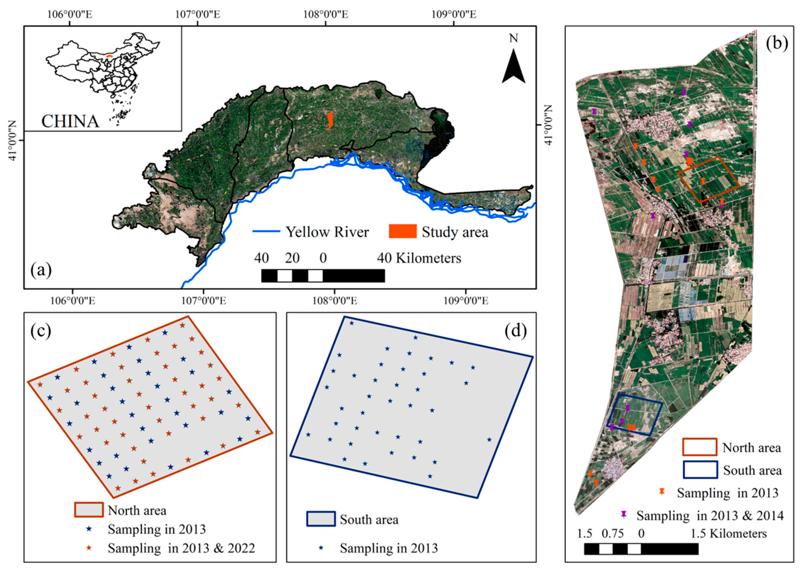
2.1. Study Area

The study area is located in the Hetao Irrigation District, China’s Inner Mongolia Autonomous Region (41°0′40″N–41°8′2″N, 107°59′33″E–108°2′5″E), as shown in Figure 1. This region is classified as an arid or semi-arid area with a typical temperate continental climate [41]. The annual precipitation ranges from 139 to 222 mm, while the annual evaporation ranges from 2200 to 2400 mm [42]. The region exhibits low rainfall and high evaporation intensity. The ground elevation ranges from 1028.6 to 1025.6 m, with flat terrain, low drainage system efficiency, and a shallow groundwater depth (with an average annual depth of 1.96 m) [43]. Combined with the implementation of long-term unreasonable irrigation practices, this has led to severe seasonal salt return and accumulation phenomena in the soil, with widespread regional salinization. The main crops in the area are oilseeds, maize, wheat, sugar beets, and forage grasses. Irrigation water mainly originates from the Yellow River (total dissolved salt (TDS) content: 0.6 g/L) [44]. The soil textures include silty loam, clay, silty clay, silty clay loam, loam, silty soil, and clay loam [45].

2.2. Materials

2.2.1. Field Sampling and Soil Salinity Measurement

This study involved multiple soil sampling campaigns in the study area in different phases during 2013, 2014, and 2022. Specifically, in 2013, six sampling events were carried out on 26 April, 7 July, 28 July, 8 August, 28 August, and 22 September. The sampling on 26 April covered regions Figure 1c,d, with a total of 115 soil samples collected. The samplings on 7 July, 28 July, 8 August, 28 August, and 22 September were concentrated in region Figure 1b, with 22 samples collected during each event. In 2014, soil sampling was conducted on 30 June, 1 August, 9 August, and 16 August. All sampling events that year were carried out at nine fixed sampling points in region Figure 1b, where repeated sampling was performed. On 26 October 2022, another round of soil salinity sampling was conducted in region Figure 1c, with a total of 44 samples collected. Based on the vegetation growth characteristics during the sampling periods, this study categorized the sampling periods into two phases: the bare soil period and the vegetation cover period. Detailed descriptions of the sampling points are provided in

Table 1. A detailed description of soil salinity sampling.

Period	Sampling Time	Sampling Number	Sampling Area
Bare soil period	26 April 2013	115	(c,d)
	22 September 2013	22	(b)
	26 October 2022	44	(c)
Vegetation cover period	7 July 2013	22	(b)
	28 July 2013	22	(b)
	8 August 2013	22	(b)
	28 August 2013	22	(b)
	30 June 2014	9	(b)
	1 August 2014	9	(b)
	9 August 2014	9	(b)
	16 August 2014	9	(b)

.

The soil samples were collected using the five-point sampling method, and the sampling point locations were recorded using a handheld GPS device. The collected soil samples were sealed and marked with a sample number and sent to the laboratory for electrical conductivity (EC, μs/cm) determination. This procedure included grinding the oven-dried soil samples and preparing a 1:5 soil–water mixture, followed by stirring, standing, settling, and filtration. Electrical conductivity of the solution was measured using a conductivity meter, and the average conductivity of five measurements was calculated. Equation (1) was used to calculate the SSC [45]:

$$\mathrm{S}\mathrm{S}\mathrm{C}=\mathrm{E}{\mathrm{C}}_{1:5}\times 0.32$$

(1)

where SSC is soil salt content, %, and EC_1:5 is electrical conductivity, μs/cm.

2.2.2. Acquisition of Remote Sensing Data

(1)

Satellite imagery

Landsat 8 and Landsat 9 satellite imagery was acquired as closely as possible to the soil sample collection dates. Image selection was based on high imaging quality and minimal cloud cover over the study area. All satellite imagery was obtained from the United States Geological Survey (USGS) (https://glovis.usgs.gov/, accessed on 31 March 2025), and the specific acquisition dates are provided in

Table 2. Dates of soil sampling and satellite imagery acquisitions.

Period	Soil Sampling Time	Image Acquisition	Row/Column	Image Source
Bare soil period	26 April 2013	20 April 2013	129/31	Landsat 8
	22 September 2013	27 September 2013	129/31
	26 October 2022	22 October 2022	129/31	Landsat 9
Vegetation cover period	7 July 2013	23 July 2013	129/31	Landsat 8
	28 July 2013	25 July 2013	129/31
	8 August 2013	10 August 2013	129/31
	28 August 2013	26 August 2013	129/31
	30 June 2014	26 June 2014	129/31
	1 August 2014	28 August 2014	129/31
	9 August 2014	13 August 2014	129/31
	16 August 2014	13 August 2014	129/31

.

(2)

In situ hyperspectral data

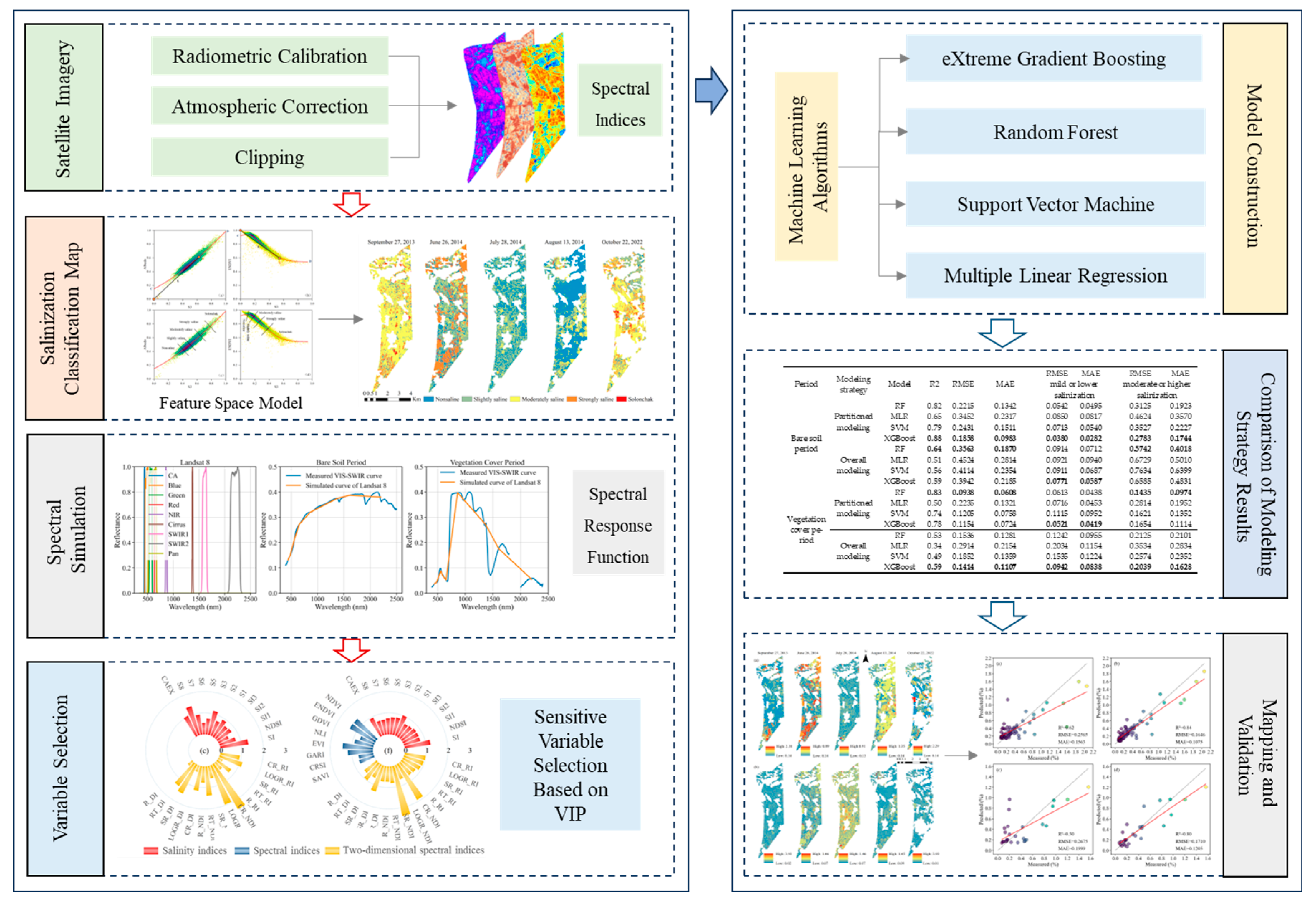
In this study, near-surface hyperspectral data were measured using an ASD AgriSpec spectrometer (Analytical Spectral Devices, Inc., Malvern Panalytical, Boulder, CO, USA) with a spectral range of 350–2500 nm and a resolution of 1 nm. The spectral data acquisition and analysis were conducted using Indico Pro software version 5.6 (ASD, Inc., Boulder, CO, USA). To reduce high-frequency noise, analysis was conducted within the spectral range of 400~2400 nm. Notably, in situ soil hyperspectral data were collected on 26 April 2013, under the conditions of low wind speed and clear, cloudless weather, with data acquisition times between 10:00 AM and 2:00 PM. Prior to measurement, the instrument was preheated for 30 min, and a built-in halogen lamp was used as the light source. The probe was positioned close to the soil surface, and calibration was performed using a white spectral panel. Each sampling point was measured 25 times, and the average value was recorded. In situ crop hyperspectral data were collected on 7 July 2013, 28 July 2013, 8 August 2013, and 28 August 2013. The measurement method was the same as that employed for the soil data, but sunlight was adopted as the light source, and the probe was positioned 1.5 m above the ground.

The in situ hyperspectral data collection at each time point was conducted simultaneously with the corresponding soil sample collection. The specific numbers of in situ soil hyperspectral and in situ crop hyperspectral data collected are detailed in Table 1.

2.3. Methods

The research process is shown in Figure 2 and includes the following key steps: (1) the acquisition and preprocessing of satellite imagery and in situ hyperspectral data; (2) the establishment of a remote sensing model for monitoring soil salinization on the basis of the spectral feature space and extraction of soil salinization classification information; (3) the conversion of satellite multispectral and in situ hyperspectral data on the basis of spectral response functions; (4) the construction of spectral indices and variable selection; (5) the comparison and analysis of the model accuracy between overall modeling and partitioned modeling approaches to determine the optimal modeling strategy for regional soil salinity remote sensing estimation; and (6) model application, mapping, and validation.

2.3.1. Soil Salinization Classification

In this study, developing a partitioned model based on the relationship between soil salinization and spectral characteristics was identified to be key to improving soil salinity prediction accuracy. Therefore, obtaining salinization classification data for the study period was essential. To achieve this, we employed remote sensing models for monitoring soil salinization based on the spectral index feature space to classify salinization degrees across the study area. In these models, selecting the appropriate spectral response parameters for saline soils is crucial for accurately extracting salinization information.

Previous studies have shown that, during both bare soil and vegetation cover periods, the soil surface spectral reflectance characteristics are influenced by salt and moisture distribution. As salinization intensifies, surface albedo (Albedo) undergoes significant changes, typically showing an increasing reflectance trend [46]. During the vegetation cover period, soil salinization has a significant impact on vegetation growth and the surface spectral properties. Higher salinity leads to greater suppression of vegetation growth, resulting in a decline in vegetation cover. Therefore, vegetation indices serve as important indirect indicators of soil salinization. The Enhanced Normalized Difference Vegetation Index (ENDVI) is an improved vegetation index used to assess vegetation cover, health, and growth dynamics [47]. Thus, in this study, Albedo and ENDVI were selected as core variables for constructing the spectral feature space. Additionally, Abbas and Khan found that the S3 index, derived from the red, green, and blue bands of remote sensing images, effectively represents soil salinization levels [48]. Therefore, we selected the S3 index as another key indicator of soil salinization. Albedo, ENDVI, and S3 are derived from Equations (2) [49], (3) [47], and (4) [48], respectively.

$$\mathrm{Albedo}=0.356\mathrm{B}2+0.13\mathrm{B}4+0.373\mathrm{B}5+0.085\mathrm{B}6+0.072\mathrm{B}7-0.0018$$

(2)

$$\mathrm{ENDVI}={\displaystyle \frac{\mathrm{B}5-\mathrm{B}4+\mathrm{B}7}{\mathrm{B}5+\mathrm{B}4+\mathrm{B}7}}$$

(3)

$$\mathrm{S}3={\displaystyle \frac{\mathrm{B}3\times \mathrm{B}4}{\mathrm{B}2}}$$

(4)

Here, B2, B3, B4, B5, B6, and B7 represent the spectral reflectance in the blue (B), green (G), red (R), near-infrared (NIR), shortwave infrared 1 (SWIR1), and shortwave infrared 2 (SWIR2) bands, respectively.

Using these spectral parameters, we developed two salinization monitoring models: the S3-Albedo spectral feature space model (denoted as SAI) for bare soil conditions and the S3-ENDVI spectral feature space model (denoted as VENS) for vegetation cover conditions. A detailed illustration of the construction of the feature space model, graphical representations, and the resulting salinization classification distribution and accuracy assessment can be found in Appendix A.

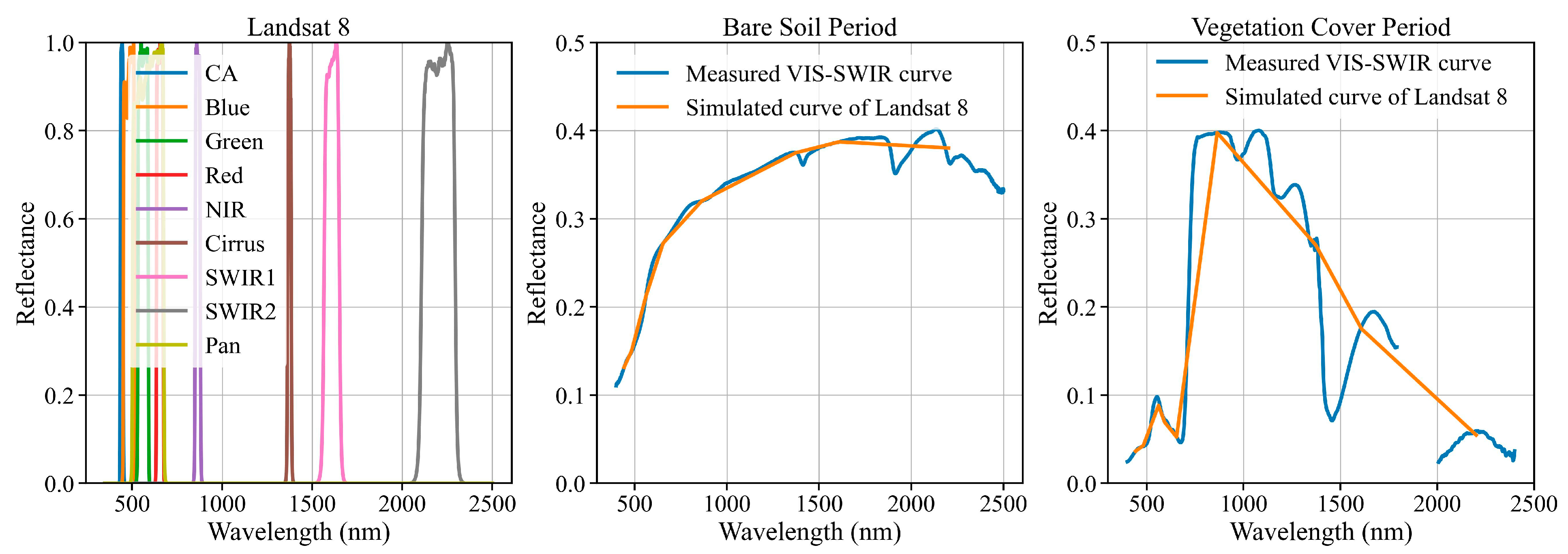
2.3.2. Spectral Simulations

The in situ hyperspectral data were converted into simulated satellite multispectral data using Equation (5) [50]:

$$R={\displaystyle \frac{{\displaystyle {\sum }_{{\lambda }_{min}}^{{\lambda }_{max}}S\left(\lambda \right)R\left(\lambda \right)}}{{\displaystyle {\sum }_{{\lambda }_{min}}^{{\lambda }_{max}}S\left(\lambda \right)}}}$$

(5)

where R is the reflectance of the simulated satellite broad band; λ_min and λ_max are the starting and ending wavelengths, respectively, of the spectrum of the satellite sensor (nm); S(λ) is the spectral response coefficient of the satellite sensor at wavelength λ; and R(λ) is the reflectance of the in situ hyperspectral data at wavelength λ.

Figure 3 shows the Landsat 8 OLI spectral response function and the simulated reflectance curves for the bare soil and vegetation cover periods, which provides the theoretical basis for converting the hyperspectral data into broad-band data. During the bare soil period, the broad-band simulated values (orange curve) closely match the in situ hyperspectral measurements (blue curve). This is especially the case within the visible to near-infrared range, where the simulated and measured values almost overlap, thus demonstrating that broad-band simulation can accurately capture the spectral characteristics of bare soil. During the vegetation cover period, the broad-band simulations still effectively reflect the spectral characteristics of the vegetation. The smooth transition feature of the Landsat 8 spectral response function renders it an effective alternative when hyperspectral data are difficult to obtain, as it can accurately capture spectral variations under different surface conditions, thereby providing a more robust estimation model.

2.3.3. Spectral Index Construction

Spectral indices can be derived by combining multiple spectral bands and are widely employed for identifying features of interest [51,52]. In soil areas with bare land or low vegetation cover, SIs are often applied as indirect indicators for monitoring salinized areas. On the basis of existing studies, 13 candidate SIs were selected. In addition, studies have shown that during the vegetation cover period, certain VIs are more sensitive to the SSC [33,34]. Therefore, 8 VIs were introduced. The spectral indices and their equations are provided in

Table 3. Spectral index calculation.

Spectral Indices		Formula	Reference
Salinity indices	SI	(B4 × B2)0.5	[53]
	NDSI	(B4 − B5)/(B4 + B5)
	SI1	(B4 × B3)0.5	[51]
	SI2	[(B5)2 + (B4)2 + (B3)2]0.5
	SI3	[(B4)2 + (B3)2]0.5
	S1	B2/B4	[48]
	S2	(B2 − B4)/(B2 + B4)
	S3	B3 × B4/B2
	S5	B2 × B4/B3
	S6	B4 × B5/B3
	S7	B6/B7	[54]
	S8	(B6 − B7)/(B6 + B7)
	CAEX	B4/B3
Vegetation indices	NDVI	(B5 − B4)/(B5 + B4)	[47]
	ENDVI	(B5 − B4 + B7)/(B5 + B4 + B7)
	GDVI	(B52 − B42)/(B52 + B42)	[55]
	NLI	(B52 − B4)/(B52 + B4)	[56]
	EVI	g × (B5 − B4)/(B5 + C1 × B4 − C2 × B2 + L)	[57]
	GARI	{B5 − [B3 + γ × (B2 − B4)]}/{B5 + [B3 + γ × (B2 − B4)]}	[58]
	CRSI	{[(B5 × B4) − (B3 × B2)]/[(B5 × B4) + (B3 × B2)]}0.5	[59]
	SAVI	[(B5 − B4) × (1 + L)]/(B5 + B4 + L)	[60]

Note: B2, B3, B4, B5, B6, and B7 represent the spectral reflectance in the blue (B), green (G), red (R), near-infrared (NIR), shortwave infrared 1 (SWIR1), and shortwave infrared 2 (SWIR2) bands, respectively. In the equations, the parameters are assigned the following values: g = 2.5, C1 = 6, C2 = −7.5, L = 1, and γ = 0.9.

.

To increase adaptability, the difference index (DI, as expressed in Equation (6)), normalized difference index (NDI, as expressed in Equation (7)), and ratio index (RI, as expressed in Equation (8)) were selected. To establish the indices, mathematical transformations such as the reciprocal transformation (1/R, RT), square root transformation (SqrtR, S), logarithmic transformation (LOG), and cosine residual transformation (CR) were applied.

$$DI(R_{\lambda i},R_{\lambda j})=R_{\lambda i}-R_{\lambda j}$$

(6)

$$NDI(R_{\lambda i},R_{\lambda j})={\displaystyle \frac{R_{\lambda i}-R_{\lambda j}}{R_{\lambda i}+R_{\lambda j}}}$$

(7)

$$RI(R_{\lambda i},R_{\lambda j})={\displaystyle \frac{R_{\lambda i}}{R_{\lambda j}}}$$

(8)

Here, R_λi and R_λj are the spectral reflectances of any two bands, with R_λi ≠ R_λj.

2.3.4. Sensitive Spectral Index Selection Method

In this study, variable importance projection (VIP) was employed to select sensitive spectral indices for the soil salinity estimation, thereby increasing the efficiency and accuracy of its construction. The VIP method is based on partial least-squares (PLS) regression, which aims to project high-dimensional data into a low-dimensional space while maximizing the correlation with target variables. The contribution of each feature is represented by its weight, W_jk, and the explained variance R_k² reflects its relevance. The VIP score (Equation (9)) combines these factors to assess feature importance. Features with VIP scores above 1 are typically considered significant, whereas those with scores below 1 may be removed on the basis of research needs [61].

$$VI{P}_j=\sqrt{{\displaystyle \frac{p\cdot {\displaystyle {\sum }_{k=1}^K{W}_{jk}^2\cdot R_k^2}}{{\displaystyle {\sum }_{k=1}^K{R}_k^2}}}}$$

(9)

Here, p represents the total number of features, W_jk² denotes the contribution weight of feature j to latent variable k, R_k² represents the explanatory power of latent variable k to the target variable, and k is the number of latent variables.

2.3.5. Soil Salinity Estimation Model Construction and Model Performance Evaluation

(1)

Soil salinity estimation model construction

Soil salinity content (SSC) estimation models were constructed using random forest (RF), extreme gradient boosting (XGBoost), support vector machine (SVM), and multiple linear regression (MLR) methods, all models were implemented in Python 3.12. The model input variables were selected based on the VIP values, retaining only variables with a VIP > 1 to reduce the impact of redundant features on modeling. Soil salinity (SSC) was used as the target variable. The models were evaluated using five-fold cross-validation, where the dataset was randomly divided into five subsets. Each subset was used as a validation set in turn, while the remaining data served as the training set, thereby enhancing the model’s generalization ability and reducing the risk of overfitting. During the bare soil period, the models were constructed using data collected on 26 April 2013, while during the vegetation cover period, data collected between 7 July and 28 August 2013, were used for model development.

The RF algorithm aims to build multiple decision trees for classification, regression, or anomaly detection. Sample subsets are generated by introducing randomness in the data and features, while features are randomly selected at each node split, thereby constructing diverse models. The trees fully grow without pruning during training, and predictions are aggregated by voting or averaging. The RF model exhibits robustness and notable generalizability, making it suitable for high-dimensional data and complex relationships, with automatic feature selection [41].

The XGBoost is an efficient gradient boosting algorithm that aims to build multiple weak learners (regression trees) in a stepwise manner, thereby employing the gradient descent method to optimize the objective function for enhanced performance. In each iteration, a new decision tree is fitted on the basis of the residuals of previous predictions; moreover, a greedy algorithm is used to obtain the optimal feature split, and a gain model is adopted to assess effectiveness. The XGBoost model introduces regularization parameters (such as tree depth, leaf count, and weight penalty) and pruning mechanisms to increase model generalizability [62].

The SVM algorithm is an ML method based on statistical learning theory that aims to construct an optimal hyperplane to maximize the classification margin. For linearly nonseparable problems, kernel methods are used to map the data into a high-dimensional space, and a linear hyperplane is constructed for nonlinear classification. Its strengths include high geometric interpretability, favorable generalization ability, and suitability for high-dimensional and small-sample problems [63].

The MLR method is a classical statistical method for analyzing the linear relationship between multiple independent variables and the dependent variable. By constructing a linear equation, the MLR method aims to quantify the effect of the independent variables on the dependent variable. It commonly uses the least-squares method to estimate model parameters, aiming to minimize the sum of squared errors between the predicted and observed values [64].

(2)

Model evaluation metrics

The model fitting performance was evaluated using the coefficient of determination (R²), root mean square error (RMSE), and mean absolute error (MAE). Generally, a higher R² value (closer to 1) and lower RMSE and MAE values indicate higher prediction accuracy.

3. Results and Analysis

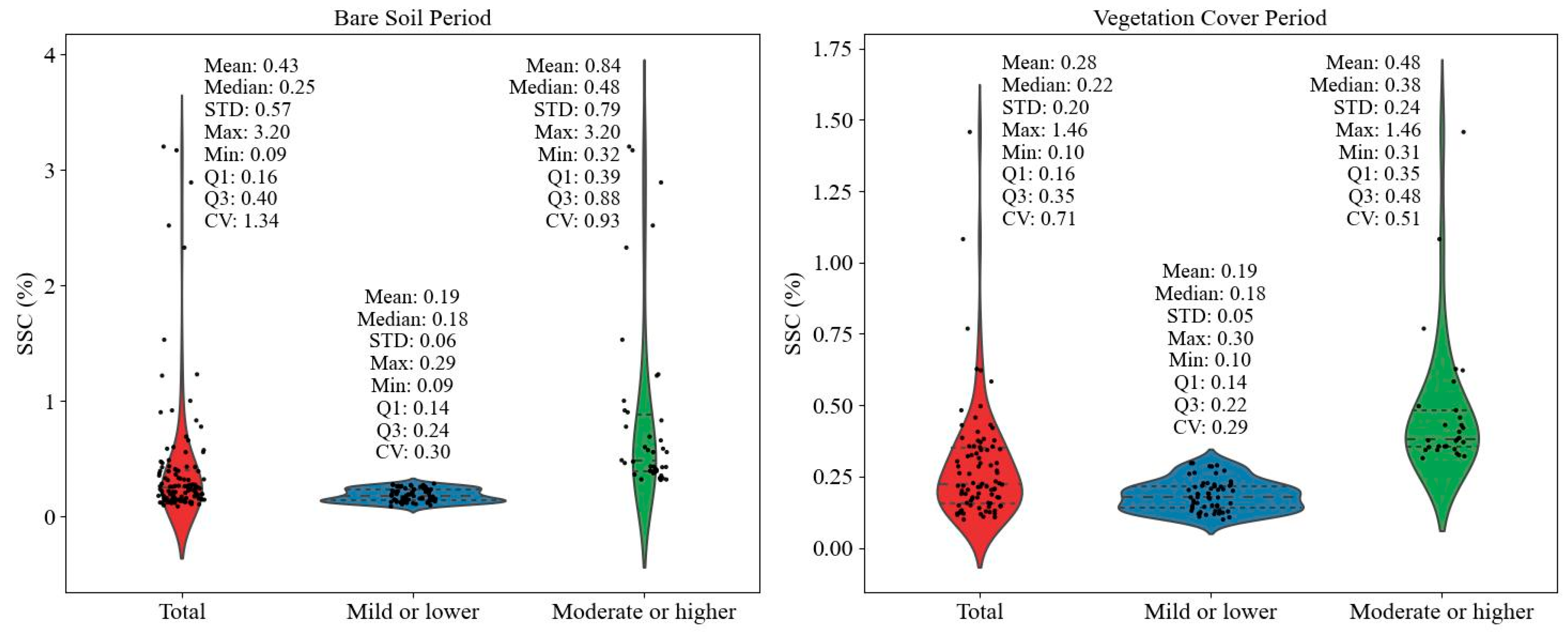
3.1. Statistical Characteristics of the Measured Soil Salinity Data

Figure 4 shows the distribution characteristics of the SSC during both the bare soil and vegetation cover periods, showing the entire dataset and different salinity degrees. During the bare soil period, the mean SSC of the total samples was 0.43%, the median was 0.25%, the standard deviation was 0.57%, and the maximum value reached 3.2%. The CV value was 1.34, indicating significant spatial heterogeneity in the salinity distribution across the sampling locations. For regions with mild or lower salinization, the mean SSC was 0.19%, with low variability (CV = 0.30), and the distribution was relatively concentrated. In contrast, for regions with moderate or higher salinization, the mean SSC was 0.84%, with a standard deviation of 0.79 and a CV value of 0.93, indicating high salinity variability. During the vegetation cover period, the mean SSC of the total samples was 0.28%, the median was 0.22%, the standard deviation was 0.20%, the maximum value was 1.46%, and the CV value was 0.71. For regions with mild or lower salinization, the mean SSC was 0.19%, with low variability (CV = 0.29), and the distribution remained relatively stable. For regions with moderate or higher salinization, the mean SSC was 0.48%, with a CV value of 0.51. The SSC clearly exhibited distinct distributions across the different salinization degrees (mild or lower salinization; moderate or higher salinization). This indicates that the dataset covers a wide range of salinity degrees (from low to high), thus providing a solid foundation of data for constructing reliable soil salinity estimation models.

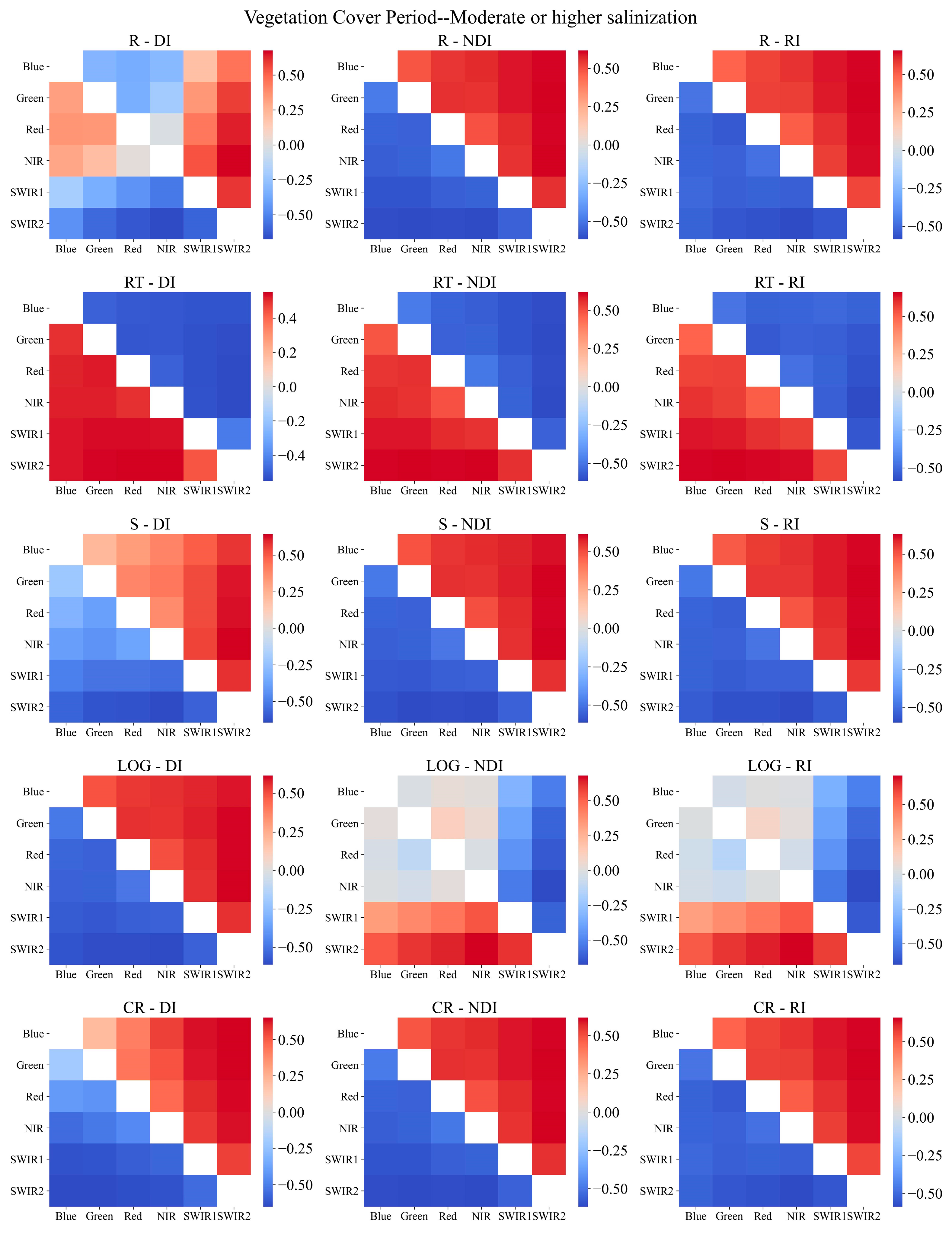
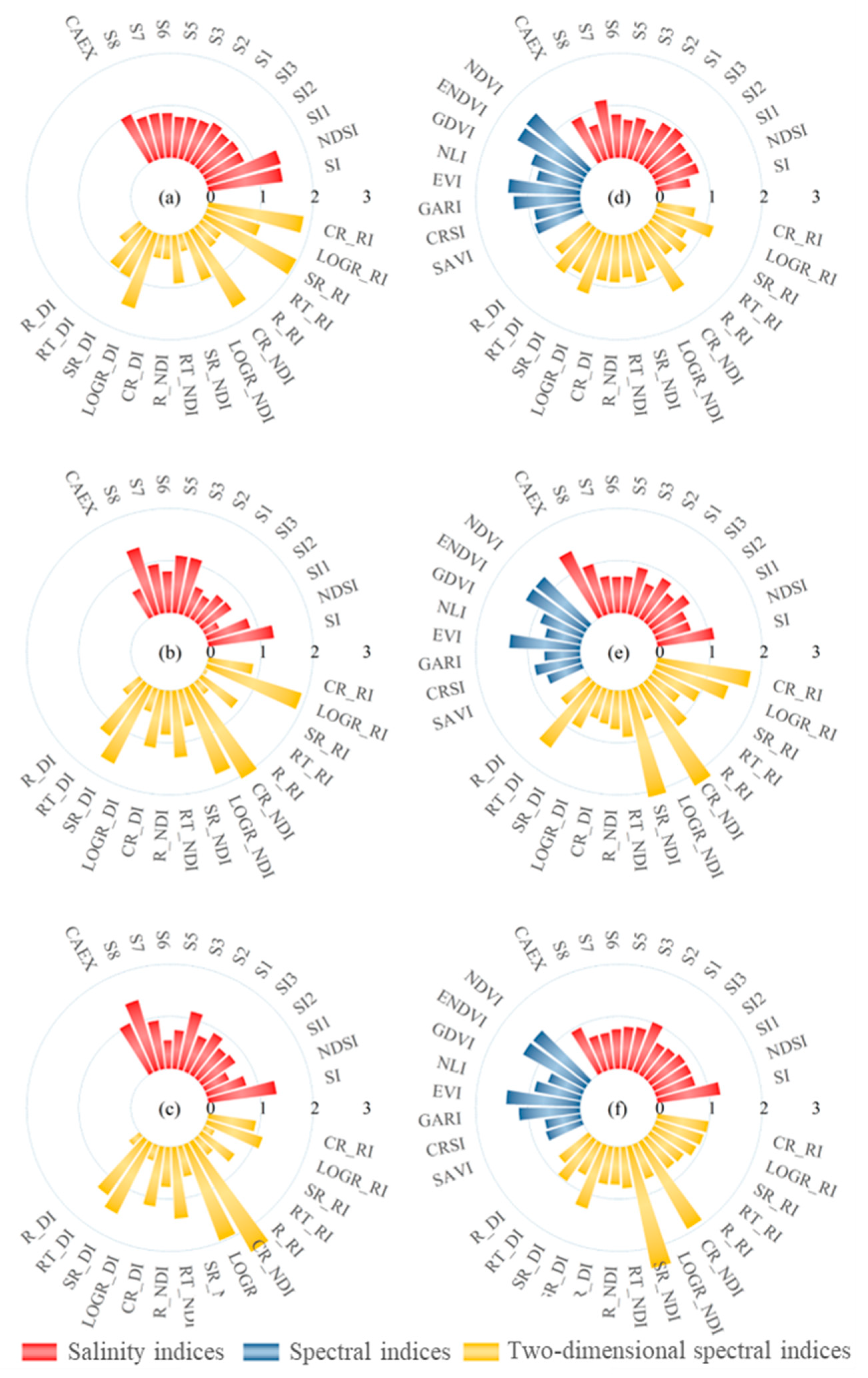
3.2. Sensitive Spectral Index Selection

To comprehensively extract spectral information, this study selected the optimal two-dimensional spectral indices under different transformation forms based on Pearson correlation coefficients (Appendix A) and combined them with traditional spectral indices as feature variables for model construction. To reduce variable redundancy, the VIP method was further employed for selection, and the VIP scores were used to visually display the importance of different spectral indices across various datasets (Figure 5). As shown in the figure, regardless of the period analyzed (vegetation cover or bare soil), two-dimensional spectral indices (e.g., NDI, DI, RI) and their transformation forms (e.g., RT, S, LOGR) exhibited consistently high VIP values across multiple datasets, significantly surpassing traditional spectral indices (e.g., SI, S8, NDVI, EVI). This indicates that transformed spectral indices can more effectively capture the spectral characteristics of soil salinization. Their construction method fully leverages the specific spectral response to soil salinization, while transformations further enhance the sensitivity of spectral feature expression, providing a reliable variable foundation for soil salinity monitoring in complex environments.

Although two-dimensional spectral indices demonstrated strong advantages, the traditional spectral indices still showed significant results. For instance, NDVI and EVI, during the vegetation cover period, as well as SI and S8, during the bare soil period, could still effectively characterize soil salinization to some extent. Furthermore, regardless of the period analyzed (bare soil or vegetation cover), the sensitivity of the spectral variables varied significantly across different datasets. Specifically, during the bare soil period, the sensitive spectral variables selected for the moderate- or higher-salinization dataset were highly consistent with those selected for the overall dataset, whereas the sensitive spectral indices for the mild- or lower-salinization dataset differed. During the vegetation cover period, no clear consistency was observed in variable selection across datasets. This suggests that directly modeling with mixed datasets containing multiple salinization degrees may obscure the differences in spectral characteristics among different salinization degrees, thereby reducing model accuracy.

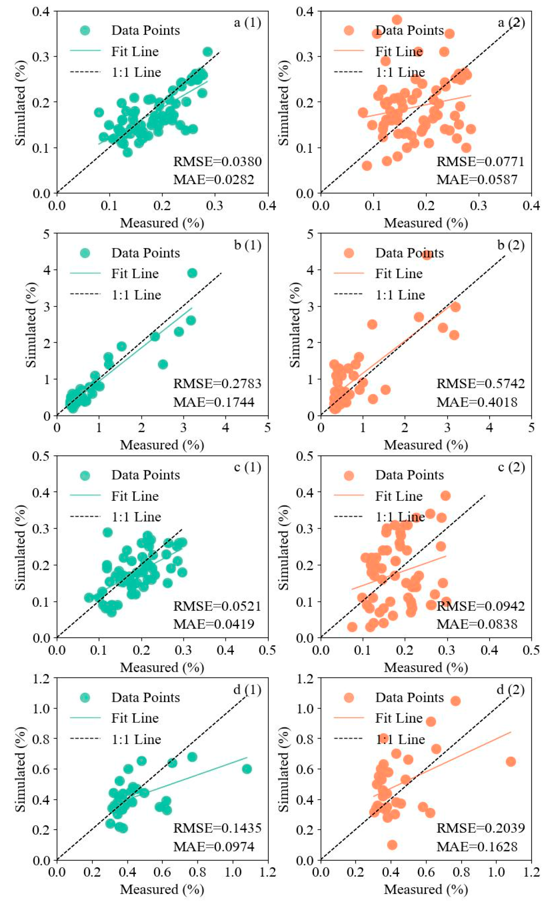
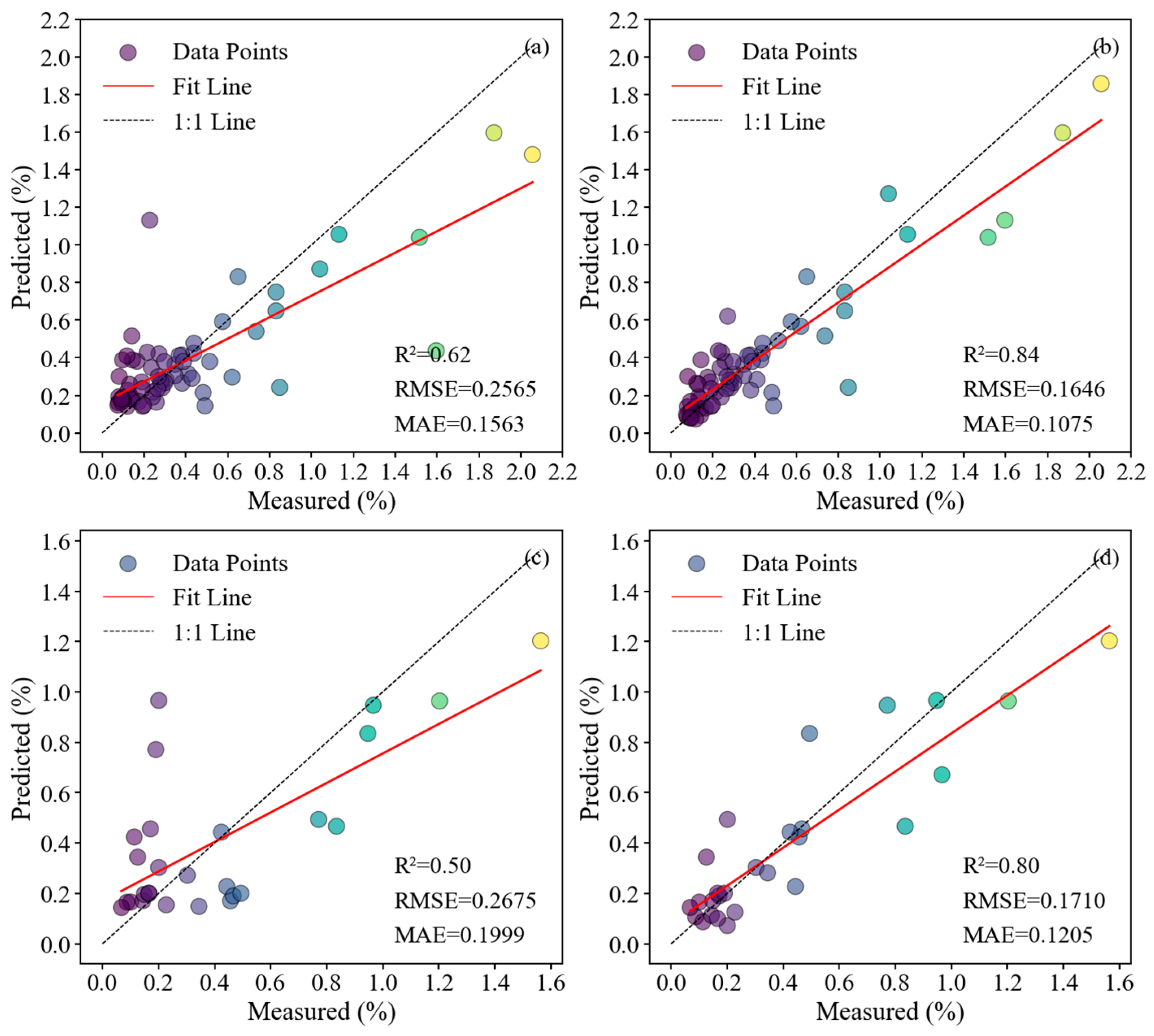
3.3. Evaluation of Soil Salinity Estimation Models with Different Modeling Approaches

To better compare the prediction performance of the partitioned and overall modeling methods, the partitioned modeling prediction results were merged, and the overall R², RMSE, and MAE values were calculated. In addition, to verify whether the use of a single model in overall modeling is suitable for the entire dataset, the overall modeling prediction results were obtained separately for different salinization degrees, with the RMSE and MAE evaluated for each salinization range. To clarify the differences in simulation effects between the partitioned and overall modeling methods during the bare soil and vegetation cover periods, the performance of partitioned modeling and overall modeling are shown in

Table 4. Performance of partitioned modeling and overall modeling.

Period	Modeling Strategy	Model	R2	RMSE	MAE	RMSE	MAE	RMSE	MAE
						Mild or Lower Salinization		Moderate or Higher Salinization
Bare soil period	Partitioned modeling	RF	0.82	0.2215	0.1342	0.0542	0.0495	0.3125	0.1923
		MLR	0.65	0.3452	0.2317	0.0850	0.0817	0.4624	0.3570
		SVM	0.79	0.2431	0.1511	0.0713	0.0540	0.3527	0.2227
		XGBoost	0.88	0.1858	0.0983	0.0380	0.0282	0.2783	0.1744
	Overall modeling	RF	0.64	0.3563	0.1870	0.0914	0.0712	0.5742	0.4018
		MLR	0.51	0.4524	0.2814	0.0921	0.0940	0.6729	0.5010
		SVM	0.56	0.4114	0.2354	0.0911	0.0687	0.7634	0.6399
		XGBoost	0.59	0.3942	0.2185	0.0771	0.0587	0.6585	0.4831
Vegetation cover period	Partitioned modeling	RF	0.83	0.0938	0.0608	0.0613	0.0438	0.1435	0.0974
		MLR	0.50	0.2235	0.1321	0.0716	0.0453	0.2814	0.1952
		SVM	0.74	0.1205	0.0758	0.1115	0.0952	0.1621	0.1352
		XGBoost	0.78	0.1154	0.0724	0.0521	0.0419	0.1654	0.1114
	Overall modeling	RF	0.53	0.1536	0.1281	0.1242	0.0955	0.2125	0.2101
		MLR	0.34	0.2914	0.2154	0.2034	0.1154	0.3534	0.2834
		SVM	0.49	0.1852	0.1359	0.1535	0.1224	0.2574	0.2352
		XGBoost	0.59	0.1414	0.1107	0.0942	0.0838	0.2039	0.1628

, respectively. As shown in the table, in most cases, the overall R² of partitioned modeling was higher than that of overall modeling, while RMSE and MAE were significantly lower, regardless of the period analyzed (bare soil or vegetation cover). For example, in the XGBoost model, during the bare soil period, the overall R² and RMSE of partitioned modeling were 0.88 and 0.1858%, respectively, whereas those of overall modeling were 0.59 and 0.3942%, respectively. These results validate the effectiveness of partitioned modeling in addressing the spatial heterogeneity in soil salinity distribution. This mainly occurs because the partitioned modeling method targets data from different salinization degrees, whereas the overall modeling method cannot accurately represent the nonlinear features of the salinity distribution, leading to greater prediction biases.

In addition, from the perspective of overall modeling, a single model cannot adequately provide optimal prediction for all salinization ranges. For example, during the bare soil period in the mild- or lower-salinization regions, the salinity prediction accuracy of the various models tested decreased in the following order: XGBoost, SVM, RF, and MLR. Moreover, in the moderate- or higher-salinization regions, the prediction accuracy of methods followed the order of RF, XGBoost, MLR, and SVM. Similarly, under partitioned modeling, the different models showed significant adaptability differences in the mild- or lower-salinization regions versus the moderate- or higher-salinization regions. For example, during the vegetation cover period, in the mild- or lower-salinization regions, the prediction accuracy of models was in the order of XGBoost, RF, MLR, and SVM (from high to low), whereas in the moderate- or higher-salinization regions, method accuracy followed the order of RF, SVM, XGBoost, and MLR. Overall, the XGBoost model outperformed the other models in most scenarios, whether in partitioned or overall modeling, with the RMSE and MAE values typically much lower than those of the other methods. For example, during the bare soil period in mild- or lower-salinization regions with partitioned modeling, the RMSE of the XGBoost model was 0.0380% and the MAE was 0.0282%, which is significantly better than the RF (RMSE = 0.0542%; MAE = 0.0495%), SVM (RMSE = 0.0713%; MAE = 0.0540%), and MLR methods (RMSE = 0.0850%; MAE = 0.0817%). However, in some scenarios (such as in moderate- or higher-salinization regions during the vegetation cover period with partitioned modeling), the RMSE and MAE of the RF model were slightly better than those of the XGBoost model. This result indicates that while the XGBoost model performs well under most conditions, the other models may be competitive in specific scenarios. This phenomenon can be attributed to the differences in model characteristics. The XGBoost model, as a decision tree-based ensemble learning method, excels at resolving nonlinear features and highly heterogeneous data, giving it a significant advantage in the mild- or lower-salinization regions. However, for datasets with lower complexity (such as that for the low-salinization region), the RF and SVM models could provide accurate predictions. In contrast, the MLR method performed significantly worse than the other models, with the highest RMSE and MAE values under most conditions, as it failed to capture the nonlinear features of the salinity distribution. This suggests that linear models (such as the MLR method) are not suitable for complex soil salinization prediction tasks, whereas nonlinear models (such as the XGBoost and RF models) are more suitable and better equipped to manage the complexity and heterogeneity of soil salinity distribution.

Scatter plots of the best prediction results under the partitioned and overall modeling approaches are shown in Figure 6. Notably, the results validate the effectiveness of partitioned modeling. For both the bare soil and vegetation cover periods, the distribution of the partitioned modeling prediction values was closer to the observed values, indicating that the model better captured the relationship between soil salinity and spectral response.

Although the overall RMSE and MAE values of partitioned modeling were lower than those of overall modeling, the former is based on predefined salinization degrees and does not account for potential errors in salinization classification that may occur in practical applications. Therefore, to ensure more accurate and practical study results, it is essential to verify the effectiveness of partitioned modeling in real-world applications.

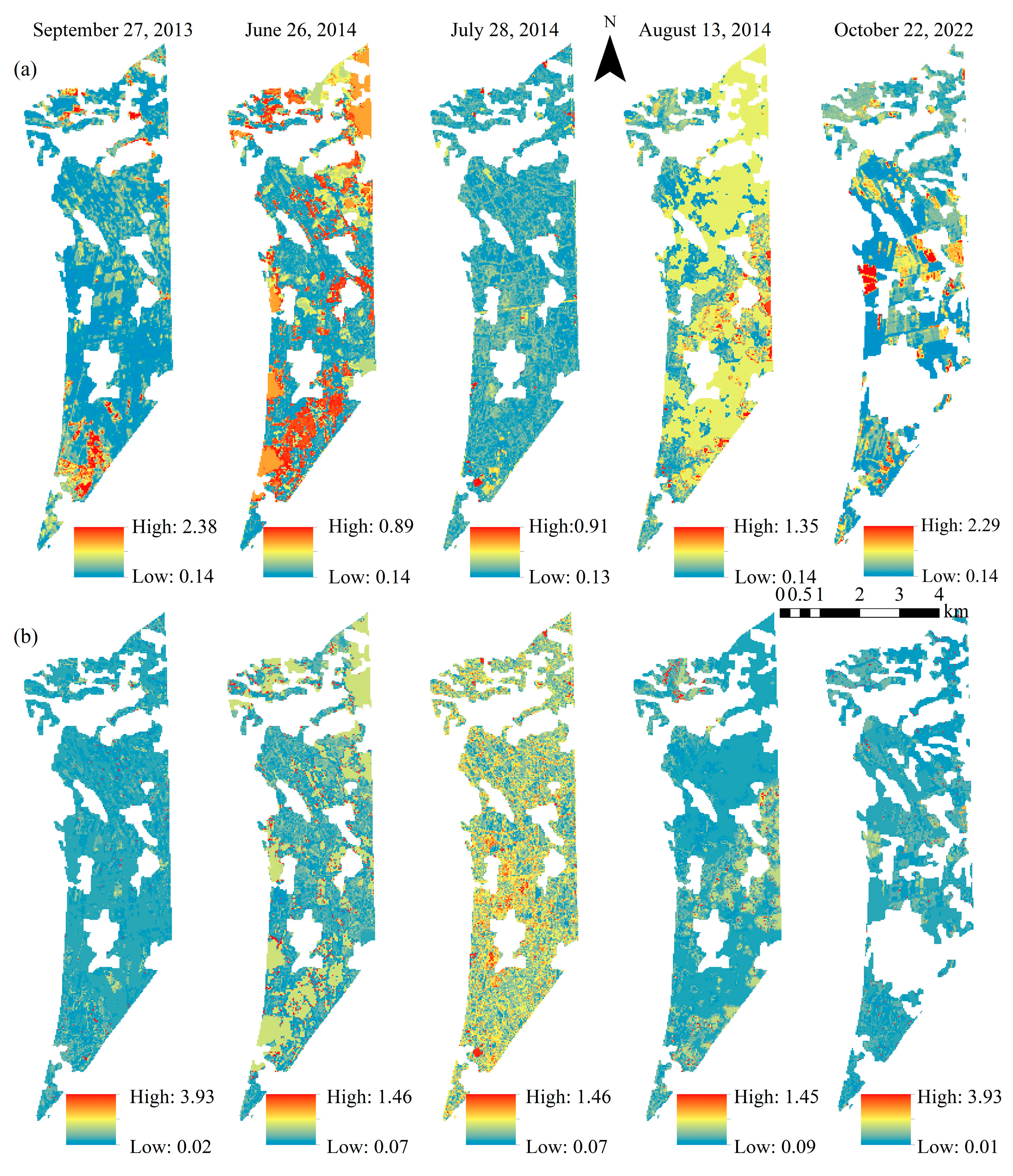
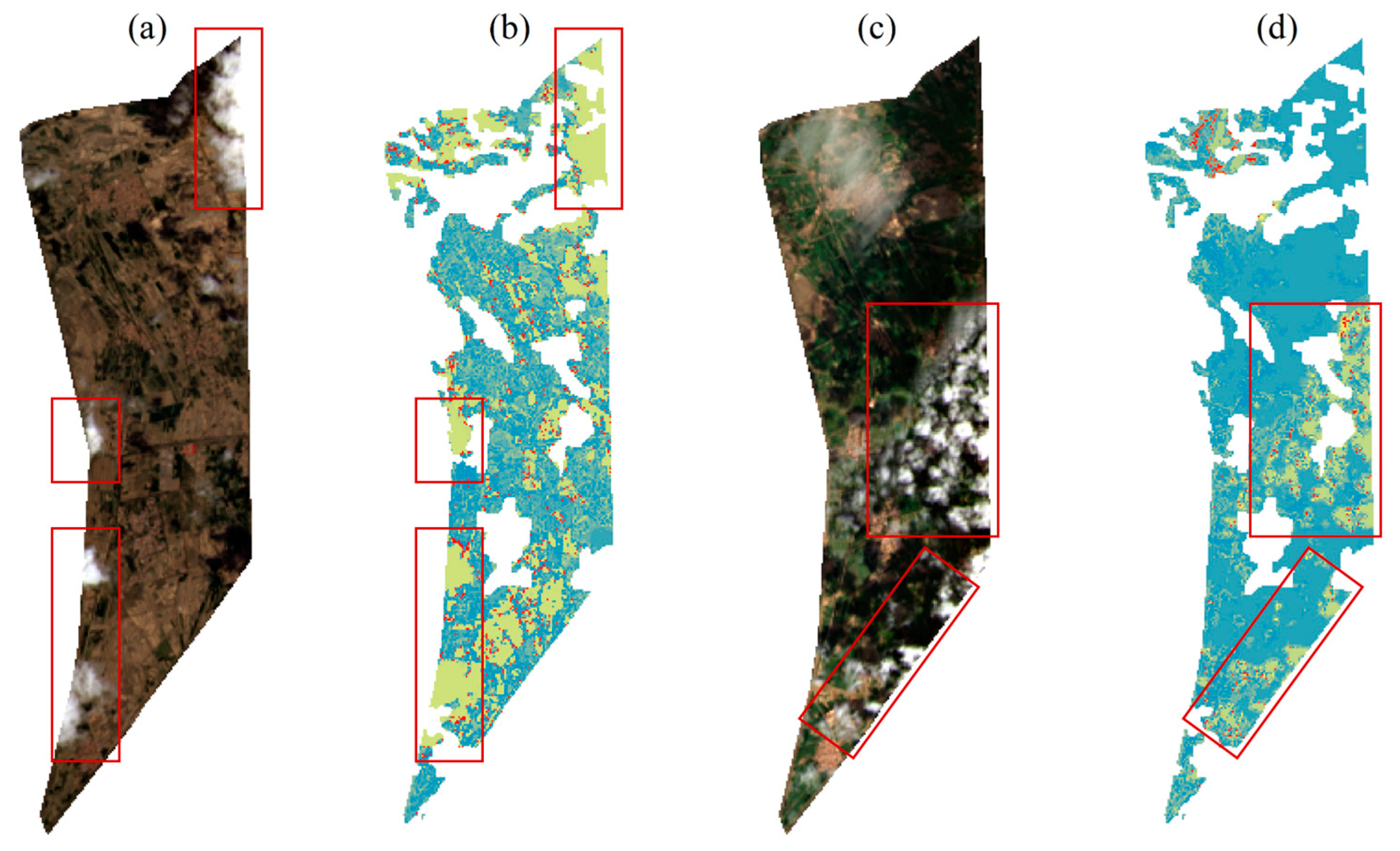
3.4. Application and Validation of Partitioned Model Based on Different Salinization Degrees

To verify the practical applicability of the proposed partitioned modeling strategy, the soil salinity distribution in the study area was predicted using the best estimation model and the corresponding salinization degree information for the given period. A comparative analysis was conducted between the estimation results obtained from partitioned modeling and those from overall modeling. Figure 7 illustrates the spatial distribution of soil salinity derived from both the overall modeling and partitioned modeling approaches in the actual application scenario. Notably, there were significant differences between the overall and partitioned modeling approaches in predicting the spatial distribution of the soil salinity, particularly in high- and low-salinity areas. In high-salinity areas, the overall modeling results clearly underestimated salinity. For example, during the bare soil periods of 27 September 2013, and 22 October 2022, the predicted salinity in high-salinity areas was clearly too low. Moreover, in low-salinity areas, the overall modeling results clearly overestimated salinity. For example, during the vegetation cover periods of 26 June 2014, and 28 July 2014, the prediction results in low-salinity areas exhibited widespread high-value saturation, indicating that the overall modeling approach lacked sensitivity to low-salinity areas and that the overall salinity values were average. Similar findings have also been reported in the study by Cui et al. [34].

In contrast, the partitioned modeling approach better predicted both high- and low-salinity areas. For example, during the bare soil periods of 27 September 2013, and 22 October 2022, the partitioned modeling method avoided the underestimation observed in the overall modeling results. Similarly, during the vegetation cover periods of 26 June 2014, and 28 July 2014, the partitioned modeling method better avoided the high-value saturation phenomenon observed in the overall modeling results. This improvement is mainly due to the consideration of differences in spectral response across varying salinization degrees in the partitioned modeling method and its targeted optimization of modeling strategies, thus effectively enhancing the preservation of intensity in high-salinity areas and increasing detail recovery in low-salinity areas.

Based on the measured sampling points, the estimation performance of overall modeling and partitioned modeling in Figure 7 was validated, and Figure 8 was further plotted to visually present the comparison results. The results indicate that even though there may be some classification errors in salinization degrees in practical applications, partitioned modeling still significantly outperformed overall modeling. For example, during the bare soil period, R² of partitioned modeling reached 0.84, with an RMSE of 0.1646% and an MAE of 0.1075%. In contrast, under the overall modeling approach, R², RMSE, and MAE were 0.62, 0.2565%, and 0.1563%, respectively, with notably higher prediction errors. This further validates the advantage of partitioned modeling in improving the accuracy of soil salinity prediction.

This result indicates that partitioned modeling can more effectively capture spectral characteristics at different degrees of salinization, significantly increasing the consistency between the model predictions and the measured values. Via modeling on the basis of the data characteristics under different salinization degrees, the partitioned modeling method reduces the prediction bias caused by neglecting salinity heterogeneity in the overall modeling method, showing greater applicability and reliability. Therefore, partitioned modeling is a more suitable strategy for salinity prediction in complex regions and provides a sound basis and practical support for accurate salinity monitoring and salinization control.

4. Discussion

(1)

Necessity of soil salinization classification during the bare soil and vegetation cover periods

Spectral characteristics provide an accurate reflection of surface material composition and micro-scale variations. In the process of soil salinization, spectral reflectance and absorption features undergo significant changes due to salt accumulation, mineral composition shifts, and variations in surface cover [1,65]. However, these effects are not uniform; instead, they systematically vary with different salinization degrees. To better understand this impact, we analyzed a selection of sensitive spectral indices across different salinization degrees. The results reveal that, in both the bare soil and vegetation cover periods, there are distinct differences in the spectral indices selected for mild- or lower-salinization degrees compared to those selected for moderate- or higher-salinization degrees. A similar conclusion was drawn by Wang et al. [66], who highlighted that soil salinity exhibits different spectral responses depending on the salinization degree. During the bare soil period, Farifteh et al. [67] and Dehaan et al. [68] found that soil spectral characteristics are primarily influenced by the composition of salt ions and mineral content. Different salinization degrees correspond to variations in dominant ion types, mineral phases, and concentrations. These compositional differences lead to distinct spectral reflectance and absorption patterns at key wavelengths. During the vegetation cover period, Cui et al. [34] also noted that soil salinity stress impacts vegetation by altering leaf pigment content, water status, and structural properties, consequently affecting vegetation spectral characteristics. As a result, vegetation in areas with different salinization degrees exhibits significantly different spectral responses. Optimizing spectral variable selection based on salinization degrees helps minimize uncertainty in overall modeling and provides a solid foundation for improving model prediction accuracy. Furthermore, the estimation results from different modeling strategies further validate the importance of classifying salinization degrees during model development. For instance, during the bare soil period, R² for the overall modeling and partitioned modeling approaches were 0.62 and 0.84, respectively. This suggests that an appropriate classification of salinization degrees allows for the identification of spectral variable combinations that are more sensitive for SSC model construction, enabling the development of estimation models that more accurately capture the unique spectral responses associated with soil salinity.

(2)

Potential of multi-source data fusion

From the perspective of remote sensing salt estimation, ground-based hyperspectral data provide significant advantages in fine-scale monitoring. With high spectral resolution, hyperspectral data can capture subtle changes in the spectral features of salinized areas, especially differences in salt crystallization formation and soil reflectance characteristics [69]. However, multispectral data, at high spatial resolution, enable coverage over large areas [70,71,72]. This complementarity provides a theoretical foundation for fine-scale and regionalized salt estimation monitoring. In this study, the advantages of both types of data were leveraged by using a spectral response function to convert ground-based hyperspectral data into wide-band features that are consistent with the multispectral satellite data, thereby enhancing the compatibility and consistency between the two datasets. It is undeniable that conversion using a spectral response function reduces the spectral resolution and information richness of the hyperspectral data, limiting their ability to capture subtle features (such as specific band responses to salt crystallization). However, hyperspectral data still retain significant advantages after simulation as multispectral data. First, hyperspectral data exhibit high pixel purity. Since each pixel contains fewer land cover types, its spectral characteristics more accurately reflect the true surface salt distribution, thus avoiding the interference of mixed-pixel effects on the modeling results and enhancing the consistency of the spectral features with the salt distribution. Second, hyperspectral data collection is highly synchronized with ground sampling. This temporal consistency is preserved after spectral-response-function-based conversion, enabling the dynamic spectral characteristics of salinized areas to be accurately captured and avoiding the uncertainty caused by a temporal lag. Although this study did not compare its results with those obtained from directly using satellite remote sensing for soil salinity estimation, previous studies have revealed that this fusion strategy not only maintains the precision of hyperspectral data but also fully utilizes the spatial coverage advantages of multispectral data. This approach significantly increases the accuracy and reliability of salt estimation models over large regional areas [13].

(3)

Prediction models and digital mapping

In this study, the performance of four models (RF, XGBoost, SVM, and MLR) in estimating soil salinity was evaluated, revealing significant differences in their predictive abilities across various salinity degrees. Overall, the SVM and MLR methods suffer limitations in managing high-dimensional data and nonlinear features, with significantly lower accuracies and applicability than the RF and XGBoost methods. This may occur because the RF and XGBoost models, as ensemble learning algorithms, can better resolve outliers, especially when analyzing the complex nonlinear spectral patterns of salinized areas. The regularization techniques in the XGBoost model in particular help minimize the impact of outliers and overfitting. In most scenarios, the XGBoost model outperformed the other models, especially in predicting samples with low salinity degrees. The XGBoost model exhibited greater prediction accuracy and stability than the RF, SVM, and MLR methods, which has also been reported previously [69]. This advantage is likely due to the ability of the XGBoost model to effectively learn and leverage the complex nonlinear relationships in low-salinity-soil data, thereby capturing low-salinity content changes through enhanced and optimized decision tree ensemble strategies. This capability is particularly beneficial in identifying slight spectral differences in low-salinity-soil environments [73,74,75,76]. However, in certain scenarios (involving moderate- or higher-salinization datasets in partitioned modeling during the vegetation cover period), the RMSE and MAE of the RF algorithm were close to or slightly better than those of the XGBoost model. This result demonstrates the adaptability differences of the different ML models in specific application scenarios, highlighting the importance of choosing the right model to increase prediction accuracy and reliability [77,78].

The core role of artificial intelligence methods is to increase estimation accuracy by fitting the complex relationship between salinity and spectral features. Nevertheless, model selection is not the sole factor determining estimation performance—the quality of the remote sensing data is also crucial. For example, on 26 June 2014, and 13 August 2014, due to persistent cloudy weather, the quality of the Landsat satellite images significantly decreased. Cloud cover caused anomalous reflectance values in the images, leading to significant overestimation of the SSC in some areas (Figure 9). This mainly occurred because the high reflectance characteristics of the clouds were similar to those of salt crystallization, and the model mistakenly interpreted the reflectance values in cloudy areas as high salinity values. This phenomenon not only affects the prediction accuracy for localized areas but also imposes a cascading effect on the estimation results for the entire region. The cloud cover issue indicates that the quality of remote sensing data cannot be ignored in estimation modeling. Therefore, increasing salt estimation accuracy requires attention to both model optimization and data quality enhancement.

(4)

Limitations and future perspectives

In large-scale soil salinity estimation, dynamic changes in environmental factors significantly affect the prediction accuracy of models. Although the salinity estimation accuracy significantly increased due to the introduction of salinization categories as prior knowledge, other key environmental factors (such as soil moisture, vegetation cover, and soil texture) can substantially affect the stability and accuracy of the estimation results [6,33,34]. For example, variations in soil moisture can alter the reflectance properties of the soil surface, vegetation cover can obscure salinity signals, and differences in soil texture affect the spectral characteristics of salt migration and accumulation. These changes in environmental factors interfere with the spectral response of salinity at different spatial and temporal scales, thus significantly increasing model uncertainty. Moreover, the interactions between environmental factors can further amplify error propagation. For example, the interaction between soil moisture and texture may alter salinity distribution characteristics [32], whereas the coupling effect of vegetation cover and salinization degrees may lead to nonlinear changes in spectral features [34]. Therefore, future research on soil salinity estimation should aim to investigate the impact of these environmental factors on monitoring accuracy and explore the applicability of these factors or features at various monitoring resolutions. However, when generating prediction distribution maps, environmental features must be visualized within the same range and resolution as the soil salinity, in addition to the spectral characteristics. This not only increases the difficulty of data collection but may also introduce cumulative errors in the distribution maps of different factors, thus affecting the accuracy of soil salinity mapping. Therefore, future research must address the issue of how to quickly and efficiently acquire high-precision spatial distribution data for other environmental factors.

5. Conclusions

In this study, a multi-source remote sensing soil salinity estimation method based on salinization-degree partitioned optimization modeling was proposed and validated. The results indicate that classifying salinization degrees can be used to identify spectral variable combinations that are more sensitive to SSC model construction, thereby positively impacting soil salinity estimation. Among spectral indices, two-dimensional spectral indices constructed through band transformations generally exhibited higher sensitivity and made more substantial contributions to predictive models compared to traditional spectral indices (VIs and SIs). Compared with overall modeling, partitioned modeling more accurately captures the specificity of spectral responses and their relationship with soil salinity, making it the preferred strategy for salinity prediction in complex regions. Specifically, during the bare soil period, the partitioned modeling approach achieved an R² of 0.84, with an RMSE of 0.1646% and an MAE of 0.1075%, significantly outperforming the overall modeling results of 0.62, 0.2565%, and 0.1563%, respectively. During the vegetation cover period, the partitioned modeling approach also demonstrated a superior performance, with R², RMSE, and MAE values of 0.80, 0.1710%, and 0.1205%, respectively, compared to the overall modeling results of 0.50, 0.2675%, and 0.1999%. These findings demonstrate that partitioned modeling more accurately reflects the spatial distribution characteristics of soil salinity, providing reliable technical support for salinization monitoring and management.

References

1. Metternicht, G.I.; Zinck, J.A. Remote sensing of soil salinity: Potentials and constraints. Remote Sens. Environ. 2003, 85, 1–20. [Google Scholar]
2. Xin, P.; Wilson, A.; Shen, C.; Ge, Z.; Moffett, K.B.; Santos, I.R.; Chen, X.; Xu, X.; Yau, Y.Y.Y.; Moore, W.; et al. Surface water and groundwater interactions in salt marshes and their impact on plant ecology and coastal biogeochemistry. Rev. Geophys. 2022, 60, e2021RG000740. [Google Scholar]
3. Chen, H.; Wu, J.; Xu, C. Monitoring Soil Salinity Classes through Remote Sensing-Based Ensemble Learning Con-cept: Considering Scale Effects. Remote Sens. 2024, 16, 642. [Google Scholar] [CrossRef]
4. Taylor, G.R.; Mah, A.H.; Kruse, F.A.; Kierein-Young, K.S.; Hewson, R.D.; Bennett, B.A. Characterization of saline soils using airborne radar imagery. Remote Sens. Environ. 1996, 57, 127–142. [Google Scholar]
5. Abbas, A.; Khan, S.; Hussain, N.; Hanjra, M.; Akbar, S. Characterizing soil salinity in irrigated agriculture using a remote sensing approach. Phys. Chem. Earth A/B/C 2013, 55–57, 43–52. [Google Scholar]
6. Scudiero, E.; Skaggs, T.; Corwin, D. Regional-scale soil salinity assessment using Landsat ETM+ canopy reflectance. Remote Sens. Environ. 2015, 169, 335–343. [Google Scholar]
7. Abuelgasim, A.; Ammad, R. Mapping soil salinity in arid and semi-arid regions using Landsat 8 OLI satellite data. Remote Sens. Appl. Soc. Environ. 2019, 13, 415–425. [Google Scholar]
8. Periasamy, S.; Ravi, K. A novel approach to quantify soil salinity by simulating the dielectric loss of SAR in three-dimensional density space. Remote Sens. Environ. 2020, 251, 112059. [Google Scholar] [CrossRef]
9. Zhang, T.; Qi, J.; Gao, Y.; Ouyang, Z.; Zeng, S.; Zhao, B. Detecting soil salinity with MODIS time series VI data. Ecol. Indic. 2015, 52, 480–489. [Google Scholar] [CrossRef]
10. Jia, J.; Chen, C.; Liu, Q.; Ding, B.; Ren, Z.; Jia, Y.; Bai, X.; Du, R.; Chen, Q.; Wang, S.; et al. Soil salinity monitoring model based on the synergistic construction of ground-UAV-satellite data. Soil Use Manag. 2024, 40, e12980. [Google Scholar] [CrossRef]
11. Fan, X.; Liu, Y.; Tao, J.; Weng, Y. Soil salinity retrieval from advanced multi-spectral sensor with partial least square regression. Remote Sens. 2015, 7, 488–511. [Google Scholar] [CrossRef]
12. Wu, S.; Wang, C.; Liu, Y.; Li, Y.; Liu, J.; Xu, A.; Pan, K.; Li, Y.; Pan, X. Mapping the salt content in soil profiles using Vis-NIR hyperspectral imaging. Soil Sci. Soc. Am. J. 2018, 82, 1259–1269. [Google Scholar] [CrossRef]
13. Cao, X.; Chen, W.; Ge, X.; Chen, X.; Wang, J.; Ding, J. Multidimensional soil salinity data mining and evaluation from different satellites. Sci. Total Environ. 2022, 846, 157416. [Google Scholar] [CrossRef] [PubMed]
14. Allbed, A.; Kumar, L.; Aldakheel, Y. Assessing soil salinity using soil salinity and vegetation indices derived from IKONOS high-spatial resolution imageries: Applications in a date palm dominated region. Geoderma 2014, 230–231, 1–8. [Google Scholar] [CrossRef]
15. Ding, J.; Yu, D. Monitoring and evaluating spatial variability of soil salinity in dry and wet seasons in the Werigan-Kuqa Oasis, China, using remote sensing and electromagnetic induction instruments. Geoderma 2014, 235–236, 316–322. [Google Scholar] [CrossRef]
16. Rahmati, M.; Hamzehpour, N. Quantitative remote sensing of soil electrical conductivity using ETM+ and ground measured data. Int. J. Remote Sens. 2017, 38, 123–140. [Google Scholar] [CrossRef]
17. Tilley, D.R.; Ahmed, M.; Son, J.H.; Badrinarayanan, H. Hyperspectral reflectance response of freshwater macrophytes to salinity in a brackish subtropical marsh. J. Environ. Qual. 2007, 36, 780–789. [Google Scholar] [CrossRef]
18. Chi, Y.; Sun, J.; Liu, W.; Wang, J.; Zhao, M. Mapping coastal wetland soil salinity in different seasons using an improved comprehensive land surface factor system. Ecol. Indic. 2019, 107, 105517. [Google Scholar] [CrossRef]
19. Peng, J.; Biswas, A.; Jiang, Q.; Zhao, R.; Hu, J.; Hu, B.; Shi, Z. Estimating soil salinity from remote sensing and terrain data in southern Xinjiang Province, China. Geoderma 2019, 337, 1309–1319. [Google Scholar] [CrossRef]
20. Geng, J.; Lv, J.; Pei, J.; Liao, C.; Tan, Q.; Wang, T.; Fang, H.; Wang, L. Prediction of soil organic carbon in black soil based on a synergistic scheme from hyperspectral data: Combining fractional-order derivatives and three-dimensional spectral indices. Comput. Electron. Agric. 2024, 220, 108905. [Google Scholar] [CrossRef]
21. Wu, W.; Zucca, C.; Muhaimeed, A.S.; Al Shafie, W.M.; Fadhil Al Quraishi, A.M.; Nangia, V.; Zhu, M.; Liu, G. Soil salinity prediction and mapping by machine learning regression in Central Mesopotamia, Iraq. Land Degrad. Dev. 2018, 29, 4005–4014. [Google Scholar] [CrossRef]
22. Fathizad, H.; Hakimzadeh Ardakani, M.A.; Sodaiezadeh, H.; Kerry, R.; Taghizadeh-Mehrjardi, R. Investigation of the spatial and temporal variation of soil salinity using random forests in the central desert of Iran. Geoderma 2020, 365, 114233. [Google Scholar] [CrossRef]
23. Peng, Y.; Liu, Z.; Lin, C.; Hu, Y.; Zhao, L.; Zou, R.; Wen, Y.; Mao, X. A new method for estimating soil fertility using extreme gradient boosting and a backpropagation neural network. Remote Sens. 2022, 14, 3311. [Google Scholar] [CrossRef]
24. Farifteh, J.; Van der Meer, F.; Atzberger, C.; Carranza, E.J.M. Quantitative analysis of salt-affected soil reflectance spectra: A comparison of two adaptive methods (PLSR and ANN). Remote Sens. Environ. 2007, 110, 59–78. [Google Scholar] [CrossRef]
25. Zhang, H.; Fu, X.; Zhang, Y.; Qi, Z.; Zhang, H.; Xu, Z. Mapping multi-depth soil salinity using remote sensing-enabled machine learning in the Yellow River Delta, China. Remote Sens. 2023, 15, 5640. [Google Scholar] [CrossRef]
26. Wang, F.; Yang, S.; Wei, Y.; Shi, Q.; Ding, J. Characterizing soil salinity at multiple depths using electromagnetic induction and remote sensing data with random forests: A case study in Tarim River Basin of southern Xinjiang, China. Sci. Total Environ. 2021, 754, 142030. [Google Scholar] [CrossRef]
27. Vermeulen, D.; Van Niekerk, A. Machine learning performance for predicting soil salinity using different combinations of geomorphometric covariates. Geoderma 2017, 299, 1–12. [Google Scholar] [CrossRef]
28. Zeraatpisheh, M.; Ayoubi, S.; Jafari, A.; Tajik, S.; Finke, P. Digital mapping of soil properties using multiple machine learning in a semi-arid region, central Iran. Geoderma 2019, 338, 445–452. [Google Scholar] [CrossRef]
29. Zeraatpisheh, M.; Ayoubi, S.; Mirbagheri, Z.; Mosaddeghi, M.; Xu, M. Spatial prediction of soil aggregate stability and soil organic carbon in aggregate fractions using machine learning algorithms and environmental variables. Geoderma Reg. 2021, 27, e00440. [Google Scholar]
30. Wang, F.; Shi, Z.; Biswas, A.; Yang, S.; Ding, J. Multi-algorithm comparison for predicting soil salinity. Geoderma 2020, 365, 114211. [Google Scholar] [CrossRef]
31. Naimi, S.; Ayoubi, S.; Di Raimo, L.A.D.L.; Demattê, J.A.M. Quantification of some intrinsic soil properties using proximal sensing in arid lands: Application of Vis-NIR, MIR, and pXRF spectroscopy. Geoderma Reg. 2022, 28, e00484. [Google Scholar] [CrossRef]
32. Xu, C.; Zeng, W.; Huang, J.; Wu, J.; van Leeuwen, W. Prediction of soil moisture content and soil salt concentration from hyperspectral laboratory and field data. Remote Sens. 2016, 8, 42. [Google Scholar] [CrossRef]
33. Zhang, J.; Zhang, Z.; Chen, J.; Chen, H.; Jin, J.; Han, J.; Wang, X.; Song, Z.; Wei, G. Estimating soil salinity with different fractional vegetation cover using remote sensing. Land Degrad. Dev. 2021, 32, 597–612. [Google Scholar] [CrossRef]
34. Cui, X.; Han, W.; Zhang, H.; Dong, Y.; Ma, W.; Zhai, X.; Zhang, L.; Li, G. Estimating and mapping the dynamics of soil salinity under different crop types using Sentinel-2 satellite imagery. Geoderma 2023, 440, 116738. [Google Scholar] [CrossRef]
35. Domínguez-Beisiegel, M.; Castañeda, C.; Mougenot, B.; Herrero, J. Analysis and map ping of the spectral characteristics of fractional green cover in saline wetlands (NE Spain) using field and remote sensing data. Remote Sens. 2016, 8, 590. [Google Scholar] [CrossRef]
36. Wang, L.; Hu, P.; Zheng, H.; Liu, Y.; Cao, X.; Hellwich, O.; Liu, T.; Luo, G.; Bao, A.; Chen, X. Integrative modeling of heterogeneous soil salinity using sparse ground samples and remote sensing images. Geoderma 2023, 430, 116321. [Google Scholar] [CrossRef]
37. Bannari, A.; El-Battay, A.; Bannari, R.; Rhinane, H. Sentinel-MSI VNIR and SWIR Bands Sensitivity Analysis for Soil Salinity Discrimination in an Arid Landscape. Remote Sens. 2018, 10, 855. [Google Scholar] [CrossRef]
38. Lv, Q.; Jiang, L.; Ma, B.; Zhao, B.; Huo, Z. A study on the effect of the salt content on the solidification of sulfate saline soil solidified with an alkali-activated geopolymer. Constr. Build. Mater. 2018, 176, 68–74. [Google Scholar] [CrossRef]
39. Ge, X.; Ding, J.; Teng, D.; Xie, B.; Zhang, X.; Wang, J.; Han, L.; Bao, Q.; Wang, J. Exploring the capability of Gaofen-5 hyperspectral data for assessing soil salinity risks. Int. J. Appl. Earth Obs. Geoinf. 2022, 112, 102969. [Google Scholar] [CrossRef]
40. Lao, C.; Yu, X.; Zhan, L.; Xin, P. Monitoring soil salinity in coastal wetlands with sentinel-2 msi data: Combining fractional-order derivatives and stacked machine learning models. Agric. Water Manag. 2024, 306, 109147. [Google Scholar] [CrossRef]
41. Wei, G.; Li, Y.; Zhang, Z.; Chen, Y.; Chen, J.; Yao, Z.; Lao, C.; Chen, H. Estimation of soil salt content by combining UAV-borne multispectral sensor and machine learning algorithms. PeerJ 2020, 8, e9087. [Google Scholar] [CrossRef] [PubMed]
42. Xiong, L.; Xu, X.; Engel, B.; Huang, Q.; Huo, Z.; Xiong, Y.; Han, W.; Huang, G. Modeling agro-hydrological processes and analyzing water use in a super-large irrigation district (Hetao) of arid upper Yellow River basin. J. Hydrol. 2021, 603, 127014. [Google Scholar] [CrossRef]
43. Du, R.; Xiang, Y.; Chen, J.; Lu, X.; Zhang, F.; Zhang, Z.; Yang, B.; Tang, Z.; Wang, X.; Qian, L. The daily soil water content monitoring of cropland in irrigation area using Sentinel-2/3 spatio-temporal fusion and machine learning. Int. J. Appl. Earth Obs. Geoinf. 2024, 132, 104081. [Google Scholar] [CrossRef]
44. Wang, G.; Shi, H.; Li, X.; Guo, J.; Wang, W.; Wu, D. Estimation of salt transport and relationship with groundwater depth in different land types in Hetao irrigation area. Trans. Chin. Soc. Agric. Mach. 2020, 51, 252–261. [Google Scholar]
45. Xu, C. Information Retrieval of Four-Dimensional Soil Moisture Content and Salt Concentration in Salted Farmland Based on Remote Sensing Data. Ph.D. Thesis, Wuhan University, Wuhan, China, 2016. [Google Scholar]
46. Liu, J.; Zhang, L.; Dong, T.; Wang, J.; Fan, Y.; Wu, H.; Geng, Q.; Yang, Q.; Zhang, Z. The applicability of remote sensing models of soil salinization based on feature space. Sustainability 2021, 13, 13711. [Google Scholar] [CrossRef]
47. Rouse, J.; Haas, R.; Schell, J.; Deering, D. Monitoring vegetation systems in the great plains with ERTS. NASA Spec. Publ. 1973, 351, 309. [Google Scholar]
48. Abbas, A.; Khan, S. Using remote sensing techniques for appraisal of irrigated soil salinity. In Advances and Applications for Management and Decision Making Land, Water and Environmental Management, Subtitle of host publication, Integrated Systems for Sustainability MODSIM07, Proceedings of the International Congress on Modelling and Simulation (MODSIM), Christchurch, New Zealand, 10–13 December 2007; Modelling and Simulation Society of Australia and New Zealand: Christchurch, New Zealand, 2007. [Google Scholar]
49. Liang, S. Narrowband to broadband conversions of land surface albedo I: Algorithms. Remote Sens. Environ. 2001, 76, 213–238. [Google Scholar] [CrossRef]
50. Trigg, S.; Flasse, S. Characterizing the spectral-temporal response of burned savannah using in situ spectroradiometry and infrared thermometry. Int. J. Remote Sens. 2000, 21, 3161–3168. [Google Scholar] [CrossRef]
51. Douaoui, A.; Nicolas, H.; Walter, C. Detecting salinity hazards within a semiarid context by means of combining soil and remote-sensing data. Geoderma 2006, 134, 217–230. [Google Scholar] [CrossRef]
52. Wang, J.; Ding, J.; Yu, D.; Ma, X.; Zhang, Z.; Ge, X.; Teng, D.; Li, X.; Liang, J.; Lizaga, I.; et al. Capability of Sentinel-2 MSI data for monitoring and mapping of soil salinity in dry and wet seasons in the Ebinur Lake region, Xinjiang, China. Geoderma 2019, 353, 172–187. [Google Scholar] [CrossRef]
53. Khan, N.; Rastoskuev, V.; Sato, Y.; Shiozawa, S. Assessment of hydrosaline land degradation by using a simple approach of remote sensing indicators. Agric. Water Manag. 2005, 77, 96–109. [Google Scholar]
54. Bannari, A.; Guedon, A.; El-Harti, A.; Cherkaoui, F.; El-Ghmari, A. Characterization of slightly and moderately saline and sodic soils in irrigated agricultural land using simulated data of advanced land imaging (EO-1) sensor. Commun. Soil Sci. Plant Anal. 2008, 39, 2795–2811. [Google Scholar]
55. Wu, W.; Al-Shafie, W.; Mhaimeed, A.; Ziadat, F.; Nangia, V.; Payne, W. Soil salinity mapping by multiscale remote sensing in Mesopotamia, Iraq. IEEE J. Sel. Top. Appl. Earth Obs. Remote Sens. 2014, 7, 4442–4452. [Google Scholar]
56. Goel, N.; Qin, W. Influences of canopy architecture on relationships between various vegetation indices and LAI and FPAR. Remote Sens. Rev. 1994, 10, 309–347. [Google Scholar]
57. Huete, A.; Didan, K.; Miura, T.; Rodriguez, E.; Gao, X.; Ferreira, L. Overview of the radiometric and biophysical performance of the MODIS vegetation indices. Remote Sens. Environ. 2002, 83, 195–213. [Google Scholar]
58. Gitelson, A.; Kaufman, Y.; Merzlyak, M. Use of a green channel in remote sensing of global vegetation from EOS-MODIS. Remote Sens. Environ. 1996, 58, 289–298. [Google Scholar]
59. Scudiero, E.; Skaggs, T.; Corwin, D. Regional scale soil salinity evaluation using Landsat 7, western San Joaquin Valley, California, USA. Geoderma Reg. 2014, 2–3, 82–90. [Google Scholar]
60. Huete, A. A soil-adjusted vegetation index (SAVI). Remote Sens. Environ. 1988, 25, 295–309. [Google Scholar]
61. Yang, N.; Yang, S.; Cui, W.; Zhang, Z.; Zhang, J.; Chen, J. Effect of spring irrigation on soil salinity monitoring with UAV-borne multispectral sensor. Int. J. Remote Sens. 2021, 42, 8952–8978. [Google Scholar] [CrossRef]
62. Chen, Z.; Jin, J.; Zhang, R.; Zhang, T.; Chen, J.; Yang, J.; Ou, C.; Guo, Y. Comparison of different missing-imputation methods for MAIAC (Multiangle Implementation of Atmospheric Correction) AOD in estimating daily PM2.5 levels. Remote Sens. 2020, 12, 3008. [Google Scholar] [CrossRef]
63. Gao, H.; Wang, C.; Wang, G.; Fu, H.; Zhu, J. A novel crop classification method based on ppfSVM classifier with time-series alignment kernel from dual-polarization SAR datasets. Remote Sens. Environ. 2021, 264, 112580. [Google Scholar]
64. Zhang, Z.; Wei, G.; Miao, H.; Wang, S.; Yang, X.; Han, J. Soil salinity inversion model based on UAV multispectral remote sensing. Trans. Chin. Soc. Agric. Mach. 2019, 50, 101–110. [Google Scholar]
65. Sun, Y.; Li, X.; Shi, H.; Ma, H.; Wang, W.; Cui, J.; Chen, C. Optimizing the inversion of soil salt in salinized wasteland using hyperspectral data from remote sensing. Trans. Chin. Soc. Agric. Eng. 2022, 38, 101–111. [Google Scholar]
66. Wang, D.; Chen, H.; Wang, Z.; Ma, Y. Inversion of soil salinity according to different salinization grades using multi-source remote sensing. Geocarto Int. 2022, 37, 1274–1293. [Google Scholar]
67. Farifteh, J.; Farshad, A.; George, R.J. Assessing salt-affected soils using remote sensing, solute modelling, and geophysics. Geoderma 2006, 130, 191–206. [Google Scholar] [CrossRef]
68. Dehaan, R.L.; Taylor, G.R. Field-derived spectra of salinized soils and vegetation as indicators of irrigation-induced soil salinization. Remote Sens. Environ. 2002, 80, 406–417. [Google Scholar]
69. Sun, M.; Liu, H.; Li, P.; Gong, P.; Yu, X.; Ye, F.; Guo, Y.; Wu, Z. Effects of salt content and particle size on spectral reflectance and model accuracy: Estimating soil salt content in arid, saline-alkali lands. Microchem. J. 2024, 207, 111666. [Google Scholar] [CrossRef]
70. Allbed, A.; Kumar, L.; Sinha, P. Soil salinity and vegetation cover change detection from multi-temporal remotely sensed imagery in Al Hassa Oasis in Saudi Arabia. Geocarto Int. 2018, 33, 830–846. [Google Scholar]
71. Guo, Y.; Zhou, Y.; Zhou, L.; Liu, T.; Wang, L.; Cheng, Y.; He, J.; Zheng, G. Using proximal sensor data for soil salinity management and mapping. J. Integr. Agric. 2019, 18, 340–349. [Google Scholar]
72. Wang, J.; Ding, J.; Yu, D.; Teng, D.; He, B.; Chen, X.; Ge, X.; Zhang, Z.; Wang, Y.; Yang, X.; et al. Machine learning-based detection of soil salinity in an arid desert region, Northwest China: A comparison between Landsat-8 OLI and Sentinel-2 MSI. Sci. Total Environ. 2020, 707, 136092. [Google Scholar] [CrossRef]
73. Ge, J.; Zhao, L.; Yu, Z.; Liu, H.; Zhang, L.; Gong, X.; Sun, H. Prediction of greenhouse tomato crop evapotranspiration using XGBoost machine learning model. Plants 2022, 11, 1923. [Google Scholar] [CrossRef] [PubMed]
74. Asselman, A.; Khaldi, M.; Aammou, S. Enhancing the prediction of student performance based on the machine learning XGBoost algorithm. Interact. Learn. Environ. 2023, 31, 3360–3379. [Google Scholar] [CrossRef]
75. Jas, K.; Dodagoudar, G. Explainable machine learning model for liquefaction potential assessment of soils using XGBoost-SHAP. Soil Dyn. Earthq. Eng. 2023, 165, 107662. [Google Scholar] [CrossRef]
76. Sun, J.; Dang, W.; Wang, F.; Nie, H.; Wei, X.; Zhang, S.; Feng, Y.; Li, P. Prediction of TOC content in organic-rich shale using machine learning algorithms: Comparative study of random forest, support vector machine, and XGBoost. Energies 2023, 16, 4159. [Google Scholar] [CrossRef]
77. Song, J.; Wang, Y.; Fang, Z.; Peng, L.; Hong, H. Potential of ensemble learning to improve tree-based classifiers for landslide susceptibility mapping. IEEE J. Sel. Top. Appl. Earth Obs. Remote Sens. 2020, 13, 4642–4662. [Google Scholar]
78. Liang, T.; Liang, S.; Zou, L.; Sun, L.; Li, B.; Lin, H.; He, T.; Tian, F. Estimation of aerosol optical depth at 30 m resolution using Landsat imagery and machine learning. Remote Sens. 2022, 14, 1053. [Google Scholar] [CrossRef]
Figure 1. Map of the study area and sampling location distribution: (a) Hetao Irrigation District; (b) study area; (c) north area; and (d) south area.
Remotesensing 17 01315 g001
Figure 2. Study flowchart.
Remotesensing 17 01315 g002
Figure 3. Landsat 8 OLI spectral response functions and simulated in situ hyperspectral broad bands.
Remotesensing 17 01315 g003
Figure 4. Descriptive statistics of soil salinity for each dataset: mean (Mean), median (Median), standard deviation (STD), extreme values (Max and Min), quartiles (Q1 and Q3), and coefficient of variation (CV).
Remotesensing 17 01315 g004
Figure 5. Feature variable selection based on the VIP feature selection method: (a), (b), and (c) represent mild or lower salinization, moderate or higher salinization, and overall dataset during the bare soil period, respectively; (d), (e), and (f) represent mild or lower salinization, moderate or higher salinization, and overall dataset during the vegetation cover period, respectively. Note: spectral indices with a VIP value greater than 1 were selected as sensitive spectral indices [61].
Remotesensing 17 01315 g005
Figure 6. Scatter plots of the soil salinity predictions based on the optimal estimation models for each salinization degree: (a), (b), (c), and (d) denote mild or lower salinization during the bare soil period, moderate or higher salinization during the bare soil period, mild or lower salinization during the vegetation cover period, and moderate or higher salinization during the vegetation cover period, respectively; (1) and (2) denote the partitioned and overall modeling approaches, respectively.
Remotesensing 17 01315 g006
Figure 7. Soil salinity spatial distribution map: (a) overall modeling approach; (b) partitioned modeling approach.
Remotesensing 17 01315 g007
Figure 8. Comparison between regional salt prediction results and measured values. (a) and (b) represent the overall and partitioned modeling approaches during the bare soil period, respectively. (c) and (d) represent the overall and partitioned modeling approaches during the vegetation cover period, respectively.
Remotesensing 17 01315 g008
Figure 9. Comparison of colored remote sensing images and estimation maps: (a) and (b) show the remote sensing image and estimation map, respectively, for 26 June 2014; (c) and (d) show the remote sensing image and estimation map, respectively, for 13 August 2014.
Remotesensing 17 01315 g009