Decadal Trends and Drivers of Dust Emissions in East Asia: Integrating Statistical and SHAP-Based Interpretability Approaches

Abstract

Dust emissions significantly impact the radiation balance, ecosystems, human health, and global climate change through long-range transport. However, their spatiotemporal characteristics and driving mechanisms in East Asia remain poorly understood. This study integrates multi-source reanalysis and remote sensing data (1980–2023) to analyze dust emissions across East Asian source regions using statistical methods and SHapley Additive exPlanations (SHAP) interpretability. The results show significant spatial and seasonal variations, with peak emissions occurring in spring (March–May). The Taklamakan Desert (S4) accounts for 38.1% of total emissions and is the largest source region. Meteorological factors are the main drivers (49.4–68.8% contribution), while climate indices contribute the least (2.9–8.0%). Wind speed is the most critical factor driving dust emissions, showing a significant positive correlation and interacting with 850 hPa geopotential height and boundary layer height. The driving factors of dust emissions vary across regions. In Mongolia (S1), dust emissions are mainly influenced by wind speed and atmospheric circulation, while in S4, near-surface meteorological conditions play a dominant role. In the Tsaidam Basin and Kumutage Desert (S5), as well as the Badain Jaran, Tengger, and Ulan Buh Deserts (S6), dust emissions are primarily driven by wind speed and boundary layer height, with atmospheric circulation also playing a certain role. Relative humidity shows a significant negative correlation with dust emissions in S5 and S6, while snowmelt and soil temperature have significant impacts on S4 and S5. The negative phases of the Arctic Oscillation and North Atlantic Oscillation enhance cold air activity and wind speed, significantly promoting dust emissions in S1 and S6. This study quantifies the mechanisms of dust emissions in East Asia and offers scientific support for improving climate models and developing disaster mitigation strategies.

1. Introduction

Dust aerosols mainly originate from arid and semi-arid regions and are one of the most important components of the atmosphere. They play a key role in the interactions and feedback processes among the environment, weather, and climate [1,2,3]. Dust aerosols account for 30% of atmospheric aerosols [4]. They significantly affect the Earth’s radiation budget through direct, indirect, and semi-direct radiative effects. By absorbing and scattering shortwave and longwave solar radiation, they alter the global radiation and heat budgets [5,6,7]. Dust aerosols can also act as cloud condensation nuclei, affecting cloud cover, cloud lifetime, and precipitation processes. Their deposition, which carries essential trace nutrients, influences biogeochemical cycles on land and in oceans [8,9].

East Asia is the second largest source of dust in the world, following the Sahara Desert, contributing approximately 10% to 25% of global dust emissions annually [10,11]. The Gobi Desert, Taklamakan Desert, and Loess Plateau are the primary dust source regions in East Asia, releasing significant amounts of dust aerosols into the atmosphere each year [12]. Research has shown that dust events in East Asia demonstrate significant seasonal variation, with over 70% of dusty weather occurring in spring and April being the most frequent month [13,14]. Meanwhile, dust storm activities in East Asia also exhibit significant long-term change characteristics. Studies have found that dust storm activities in East Asia have shown a significant weakening trend over the past few decades, which is closely related to increased precipitation and improved vegetation cover under global warming [15,16]. Other research has pointed out that the frequency and intensity of dust storms in major global dust source regions have shown decadal variations over the past few decades, and these variation patterns have complex connections with regional climate change and human activities [17,18]. Regarding climate impacts, research suggests that atmospheric dust significantly affects regional and global climate systems through direct and indirect radiative forcing [19,20]. Further studies have indicated that East Asian dust not only alters regional radiation balance and precipitation distribution but also has important impacts on the North Pacific ecosystem through long-distance transport [10].

The driving mechanisms of dust emission and transport are highly complex and influenced by meteorological conditions, surface characteristics, large-scale atmospheric circulation, and climate teleconnection factors. Among meteorological conditions, wind speed is the most direct driving factor, providing the energy to lift dust from the surface into the atmosphere [21,22]. Precipitation suppresses dust emissions by increasing soil moisture, while dry weather enhances dust activity [23,24]. Temperature changes indirectly affect dust emissions by accelerating soil moisture evaporation, while snowmelt and freeze–thaw processes during winter and spring alter surface roughness, further influencing dust emission potential [25,26]. Surface conditions, such as soil moisture, vegetation cover, and snowmelt processes, significantly regulate dust emissions by affecting material availability and surface stability in dust source regions [27,28]. Moreover, there are complex interactions between meteorological conditions and surface characteristics. For instance, precipitation not only increases soil moisture but also indirectly suppresses dust emissions by promoting vegetation growth [29]. Large-scale atmospheric circulation and climate teleconnection factors are also critical in regulating dust activity. Features such as the 500 hPa geopotential height field, the westerly jet, and the mean sea level pressure (MSLP) indirectly control dust activity in East Asia by influencing regional weather conditions [30,31]. Mao et al. [32] found that the negative phase of the Arctic Oscillation (AO) enhances cold air activity over the Mongolian Plateau, leading to an increase in the frequency of dust storms in East Asia. Gong et al. [33] indicated that the positive phase of the North Atlantic Oscillation (NAO) strengthens the westerly jet stream, facilitating long-range dust transport, while the positive phase of the Antarctic Oscillation (AAO) alters the Southern Hemisphere circulation pattern, indirectly affecting cold air activity in the Northern Hemisphere [34]. Additionally, ENSO events modulate the East Asian monsoon and precipitation patterns, influencing dust emission and transport pathways [35,36].

Although numerous studies have explored the impacts of various meteorological factors and surface conditions on dust emissions, several critical limitations remain in current research. First, most studies tend to focus on the role of individual factors, lacking a systematic analysis of the combined effects of multiple factors. Second, the relative contributions of different factors to dust emissions have not been fully quantified, and the combined contributions of different categories of driving factors remain significantly uncertain. In terms of research methods, previous studies on dust emissions have primarily relied on numerical simulation tools, such as DREAM, RegCM4, and WRF-Chem [37,38,39], combined with satellite remote sensing data from MODIS, CALIPSO [18,40], and ground-based observations. However, these approaches face limitations in addressing parameter heterogeneity, dynamic source changes, and transboundary dust transport [41,42]. Traditional dust emission models often treat potential dust sources as static distributions, overlooking the dynamic changes in dust sources caused by climate change and human activities. Moreover, the quantitative evaluation of contributions from foreign source regions, such as Mongolia, to East Asian dust emissions remains insufficient. Although satellite remote sensing technology has supported dust monitoring, limitations in spatial and temporal resolution, as well as challenges such as cloud interference, constrain the accuracy of dust identification and tracking.

To address the aforementioned issues, this study utilizes the Modern-Era Retrospective Analysis for Research and Applications, version 2 (MERRA-2) reanalysis dataset as the core data source [43,44]. This dataset integrates multi-satellite observation systems and AERONET ground-based monitoring network data to provide more continuous, consistent, and comprehensive dust emission information, establishing a solid foundation for systematic analysis in this research. Furthermore, this study introduces the SHAP method as a core analytical tool that is based on game theory principles and can effectively handle complex non-linear relationships and multi-level interactions between variables, allocating precise contribution values to each predictor, thereby revealing the quantitative impact of various driving factors on dust emissions [45,46,47]. The SHAP method demonstrates exceptional performance when dealing with highly correlated predictor variables capable of distinguishing between the independent contributions and synergistic effects of various factors, which is crucial for deciphering the complex driving mechanisms of dust emissions. This paper analyzes the spatiotemporal variations of dust emissions in East Asian dust source regions using the MERRA-2 dataset, systematically revealing long-term trends and regional differences. It then evaluates the contributions of key influencing factors to East Asian dust emissions and their interaction mechanisms across various dust source regions based on the SHAP method combined with traditional statistical analysis. This comprehensive analytical approach not only enables in-depth exploration of the complex interactions between different factors and their regulatory mechanisms on dust emissions but will also provide solid scientific evidence and theoretical support for accurately predicting and effectively controlling future dust activities in the East Asian region.

The remainder of the paper is organized as follows: Section 2 presents the basic characteristics of the study area, the data sources, and the specific research methods. Section 3 describes the spatiotemporal distribution characteristics of dust emissions in East Asia from 1980 to 2023, quantifies the relative contributions of various factors, and provides a detailed analysis of the spatiotemporal correlations between key factors and dust emissions. Section 4 includes a discussion covering the strengths, limitations, and future research directions of the study. Finally, Section 5 summarizes the conclusions of the study.

2. Materials and Methods

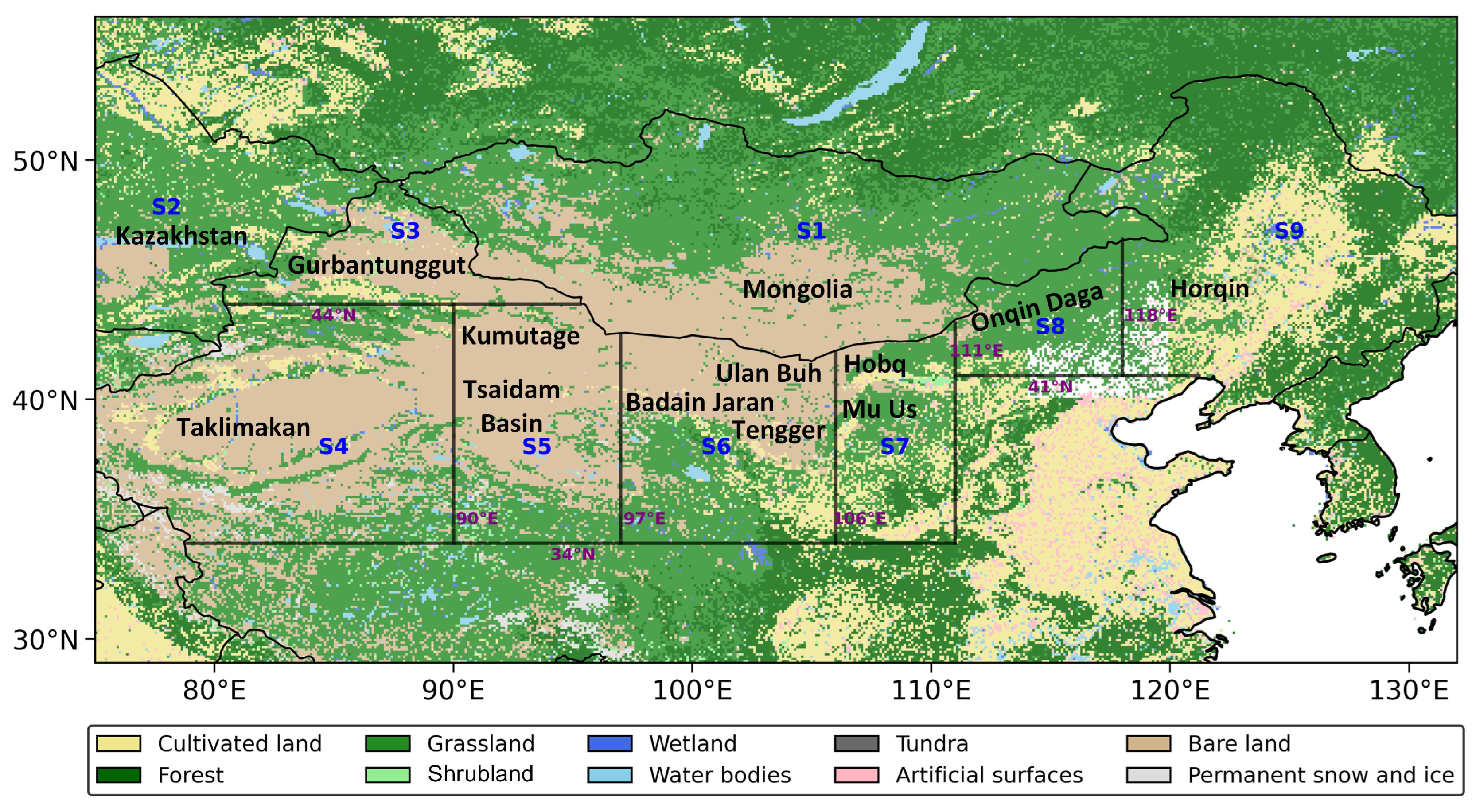
2.1. Study Area

Figure 1 presents the land cover types in the major dust source regions of East Asia (26°N–56°N, 74°E–132°E) based on the GlobeLand30 dataset, a 30 m resolution global land cover product developed by the National Geomatics Center of China (see Section 2.2.1). The GlobeLand30 dataset classifies land cover into 10 categories: cultivated land, forest, grassland, shrubland, wetland, water bodies, tundra, artificial surfaces, bare land, and permanent snow and ice. In Northeast China, forests and croplands dominate the landscape, while grasslands and croplands are prevalent in North China. In the inland regions of Northwest China, the terrain primarily consists of grasslands, bare land, and shrublands characterized by low vegetation cover. Deserts and gobi areas in East Asia are mainly distributed in bare land regions, which not only serve as the principal dust sources in East Asia but are also significant dust sources on a global scale. According to the classification by Zhang et al. [10], the East Asian dust source regions are divided into nine sub-regions (Figure 1). Some of these dust source regions are located outside China, including Mongolia (S1) and eastern Kazakhstan (S2), while S3–S9 encompass the major desert and sandy land areas within China. The contribution of dust emissions from each sub-region varies significantly. The Taklimakan Desert (S4), China’s largest mobile desert (covering an area of approximately 33.7 × 10⁴ km²), has high-intensity dust emissions mainly driven by frequent cold air fronts in spring and the loose sandy surface of the desert. The Gobi Desert in southern Mongolia (S1) is the most significant dust source outside China, with dust emissions primarily affected by low vegetation coverage caused by overgrazing and climate change. Regions S5 and S6 experience fewer dust events, but these events have severe impacts, and large amounts of dust particles are easily transported to the troposphere and downwind regions, making them major dust source regions in East Asia as well. The remaining regions, such as S3, S7, S8, and S9, contribute relatively less, mainly due to their surface characteristics, vegetation coverage conditions, and human activities.

2.2. Remote Sensing Data

2.2.1. GlobeLand30

GlobeLand30 is an open-access global land cover dataset with a 30 m spatial resolution, developed by the National Geomatics Center of China. This dataset was extracted from more than 20,000 Landsat, China HJ-1 satellite, and GF-1 satellite images. The dataset contains 10 major land cover types: cultivated land, forest, grassland, shrubland, wetland, water bodies, tundra, artificial surfaces, bare land, and permanent snow and ice. GlobeLand30 is an important outcome of the Global Land Cover Mapping and Key Techniques Research Project under China’s National High-tech R&D Program (863 Program). These datasets are highly valuable for monitoring environmental changes and resource management at global, regional, and local scales [48,49].

2.2.2. NDVI

The normalized difference vegetation index (NDVI) data used in this study are derived from NOAA’s Climate Data Record (CDR) and are calculated from surface reflectance products generated by AVHRR and VIIRS sensors. The calculation formula for NDVI is as follows:

$$NDVI={\displaystyle \frac{NIR-RED}{NIR+RED}}$$

where NIR represents the reflectance in the near-infrared band, and RED represents the reflectance in the red band. The NDVI value ranges from −1 to 1, and it is commonly used to measure vegetation coverage. Higher NDVI values typically indicate denser and healthier vegetation, while lower but still positive NDVI values may indicate vegetation in a drier state or with reduced leaf moisture content, rather than merely sparse vegetation. Values near zero or negative typically represent areas with no vegetation coverage. Specifically, NDVI data before 2014 (1981–2013) are based on surface reflectance from Channels 1 and 2 of the Advanced Very High-Resolution Radiometer (AVHRR) onboard NOAA polar-orbiting satellites, with wavelengths of 630 nm and 865 nm, respectively. NDVI data from 2014 onwards (2014 to 10 days prior to the current date) are based on surface reflectance from Channels I1, I2, and I3 of the Visible Infrared Imaging Radiometer Suite (VIIRS), with wavelengths of 640 nm, 865 nm, and 1610 nm, respectively. Both datasets are gridded with a spatial resolution of 0.05° × 0.05° and provide globally covered daily averages. This dataset is jointly produced by NASA’s Goddard Space Flight Center (GSFC) and the University of Maryland (UMD) and is delivered in netCDF-4 file format compliant with ACDD and CF conventions [50,51].

2.3. Reanalysis Data

2.3.1. MERRA-2

MERRA-2 (The Modern-Era Retrospective Analysis for Research and Applications, version 2), developed by NASA’s Global Modeling and Assimilation Office (GMAO), is a high-resolution global atmospheric reanalysis product designed for the satellite era. Based on the Goddard Earth Observing System Data Assimilation System (GEOS-DAS), MERRA-2 integrates the GEOS-5 climate model and the GSI analysis scheme. Its aerosol model employs a coupled version of the GOCART model to simulate the sources, sinks, and chemical properties of 15 aerosols, including dust, sea salt, and black carbon [43]. MERRA-2 significantly enhances the accuracy and reliability of aerosol reanalysis by integrating multiple data sources (such as MISR, MODIS, and AERONET) [52]. MISR provides precise aerosol optical depth (AOD) data with high spatial resolution, though it is limited by shorter temporal coverage [53]. AERONET, through high-precision ground-based observations, provides crucial validation data for MERRA-2, playing an important role, particularly in dust classification and transport pathway studies [54].

Dust emissions in MERRA-2 are parameterized based on a climatological map of potential dust source regions, linking dust-emitting areas to topographic depressions. Dust emissions are divided into five size bins (bin001 to bin005, with particle radii ranging from 0.1 to 10 μm), all of which are wind-driven [55,56]. MERRA-2 data span from 1980 to the present, with a spatial resolution of 0.625° × 0.5°and a temporal resolution ranging from hourly to monthly. This study utilizes the monthly dust emissions data from the dataset “tavgM_2d_adg_Nx”. Dust emissions are calculated as shown in Equation (1):

Dust Emissions (DUEM) = Dust Emission Bin001 + Dust Emission Bin002 +
Dust Emission Bin003 + Dust Emission Bin004 + Dust Emission Bin005

(1)

Multiple studies have validated the reliability and advantages of the MERRA-2 dust emission dataset. Jing et al. [57] demonstrated that MERRA-2 can quantitatively estimate the dust budget of extreme dust events by comparing it with the AeroCom multi-model ensemble. Yao et al. [58] found that MERRA-2 performs exceptionally well in estimating dust emissions and deposition and is effective in quantifying the dust balance. Shi et al. [59] showed that the interannual variability of MERRA-2 dust emissions is consistent with research findings from 1980 to 2018 across global dust source regions, highlighting its accuracy in reflecting long-term trends. Wang et al. [12] observed a significant positive correlation between MERRA-2 dust emissions and lower atmospheric dust concentrations obtained from CALIPSO, with both exhibiting consistent long-term trends. These studies collectively confirm that the MERRA-2 dataset is reliable and suitable for quantitatively estimating global or regional dust emissions and analyzing their long-term variations.

2.3.2. GLDAS

The monthly soil moisture (MSoil), soil temperature (TSoil), bare soil evaporation (ESoil), and snow melt (SM) data from 1980 to 2023 are sourced from the NASA Global Land Data Assimilation System (GLDAS), with a spatial resolution of 0.25° × 0.25° [60,61]. GLDAS employs advanced land surface models and data assimilation techniques to generate optimal land surface states and flux fields based on satellite and ground-based observation data [62]. GLDAS supports multiple offline land surface models, integrates a large volume of observational data, and operates globally at high resolution with the assistance of the Land Information System (LIS).

2.3.3. ERA5

ERA5, the fifth-generation global reanalysis dataset developed by the European Centre for Medium-Range Weather Forecasts (ECMWF), has effectively superseded its predecessor ERA-Interim and has become the most widely used dataset in weather and air quality simulation research [63]. This study employs monthly ERA5 reanalysis data from 1980 to 2023 with a high spatial resolution 0.25° × 0.25° grid structure. The key meteorological variables analyzed include 10 m wind speed (WS), relative humidity (RH), 2 m air temperature (T), total precipitation (TP), 500 hPa geopotential height (GH_500), 850 hPa geopotential height (GH_850), boundary layer height (BLH) and sea level pressure (SLP) [64,65]. The ERA5 dataset offers high spatiotemporal resolution, multi-variable support, and long-term continuity [66]. It accurately captures wind fields, humidity, precipitation and atmospheric circulation, temperature, surface pressure, and other meteorological variables in dust source regions [67,68,69,70]. It effectively represents the key meteorological factors driving dust emission and long-range transport, providing strong data support for building efficient dust emission models and assessing their climate effects.

2.4. Climate Indices

The datasets for the Arctic Oscillation (AO), Antarctic Oscillation (AAO), North Atlantic Oscillation (NAO), and El Niño–Southern Oscillation (ENSO, represented by the Niño 3.4 index) were obtained from the Climate Prediction Center of the National Oceanic and Atmospheric Administration (NOAA/CPC) and can be accessed at https://origin.cpc.ncep.noaa.gov (accessed on 1 February 2025).

2.5. Methods

2.5.1. Theil–Sen Median Trend Analysis and the Mann–Kendall Test

The Mann–Kendall test is commonly used to detect the presence of trends in time series data [71,72], especially in environmental studies. This test can be considered a non-parametric alternative to testing the null hypothesis of zero slope in a linear regression between the time series data and time. Regarding the results, a negative Z-value indicates a decreasing trend, while a positive Z-value indicates an increasing trend. At a significance level of 0.05 (or 0.01, 0.001), Z >1.96 (or 2.58) and Z < − 1.96 (or −2.58) represent significant increasing and decreasing trends, respectively (

Table 1. Categories of trends based on Theil–Sen median and Mann-Kendall test.

Label	Z Value	Trend Categories
β > 0	Z > 2.58	Extremely significant increase
	1.96 ≤ Z ≤ 2.58	Significant increase
	1.65 ≤ Z ≤ 1.96	Slightly significant increase
	Z ≤ 1.65	No significant increase
β = 0	Z	No change
β < 0	Z ≤ 1.65	No significant decrease
	1.65 < Z ≤ 1.96	Slightly significant decrease
	1.96 < Z ≤ 2.58	Significant decrease
	Z > 2.58	Extremely significant decrease

). The Theil–Sen method is a non-parametric alternative to ordinary least squares regression. Compared to linear regression, the advantage of the Sen slope lies in its robustness against outliers and data errors [73,74]. The formula for the Sen slope is as follows:

$$\beta =Median\left({\displaystyle \frac{x_j-x_i}{i-j}}\right)$$

where $x_i$ and $x_j$ are the data values at times $j$ and $i$ ($j$ > $i$), respectively, and β represents the Theil–Sen median slope. When β > 0, it indicates an increasing trend; conversely, when β < 0, it indicates a decreasing trend. Below is the table of trend categories based on Theil–Sen median analysis and the Mann–Kendall test, detailing the significance of trends according to different Z-value ranges and the sign of the slope (β):

2.5.2. XGBoost Regression and SHAP Values

XGBoost (Extreme Gradient Boosting) is an efficient ensemble learning algorithm based on Gradient Boosting Decision Trees (GBDT) [75]. Due to its high predictive accuracy and computational efficiency, it has been widely applied to large-scale datasets and complex nonlinear problems. Compared to traditional GBDT, XGBoost introduces several key improvements [76,77]. First, a regularization term is added to the objective function, effectively reducing overfitting and improving generalization performance. Second, the process of searching for feature split points is optimized using parallel computing, significantly accelerating training. Furthermore, XGBoost includes built-in mechanisms to handle missing values and supports user-defined objective functions, making it highly flexible for tasks such as classification and regression. In pollutant emission modeling and prediction, where the spatiotemporal distribution of pollutants is often influenced by complex nonlinear factors, XGBoost captures intricate relationships between variables by iteratively fitting residuals.

The analyzed near-surface meteorological factors include WS, RH, T, BLH, and TP. Surface conditions cover the NDVI, Esoil, Msoil, Tsoil, and SM. Atmospheric circulation factors include MSLP, GH_500, and GH_850. Additionally, climate indices such as the AO, NAO, AAO, and ENSO are also included.

In this study, to ensure the generalization ability of the model and effectively address the temporal dependency of time series data, we adopted the Expanding Window validation method for model evaluation. During the Expanding Window process, the initial training set contains 15% of the data, and the training set gradually expands over time, adding one data point at a time while using the most recent data for testing. This method ensures that the model does not use future data for training, thereby preventing data leakage and allowing for a more realistic simulation of actual forecasting scenarios. It is particularly suitable for long-term trend prediction. The model performance is evaluated using multiple metrics, including the coefficient of determination (R²), Root Mean Square Error (RMSE), and Mean Absolute Error (MAE). The final model performance is assessed based on a comprehensive evaluation of all predictions made throughout the Expanding Window process.

Although XGBoost performs exceptionally well in handling high-dimensional data and complex nonlinear relationships, its intricate structure often leads to it being regarded as a “black box”, making it challenging to interpret the specific contributions of individual features to predictions. To address this issue, SHAP (SHapley Additive exPlanations) is introduced in this study. SHAP is based on Shapley value theory from game theory [45], originally proposed by Lloyd Shapley in the early 1950s, which provides a theoretical foundation for quantifying the relative contributions of various factors in multivariate systems. The core idea of SHAP is to treat the model output as the result of all features working together and to construct an additive explanation model that fairly distributes the contribution of each feature to the predicted value, thereby quantifying feature importance and its relationship to the target variable [78,79]. Although the computation of Shapley values presents challenges in terms of computational complexity, SHAP significantly reduces the computational cost through innovative algorithms (such as Tree SHAP), making it applicable to large-scale datasets and complex models [46]. To further analyze the relative importance of different features to the target variable, the relative contribution of each feature is calculated based on SHAP values. The calculation formula is as follows:

$${\mathrm{S}\mathrm{H}\mathrm{A}\mathrm{P}}_r={\displaystyle \frac{{SHAP}_i}{{SHAP}_{total}}}$$

where ${\mathrm{S}\mathrm{H}\mathrm{A}\mathrm{P}}_r$ represents the relative contribution of an input feature, ${SHAP}_i$ is the sum of absolute SHAP values for a given input feature, and ${SHAP}_{total}$ is the sum of absolute SHAP values for all input features. The introduction of relative contribution aims to provide a more intuitive comparison of the impact of different features on the prediction results, especially in high-dimensional data [80].

3. Results

3.1. Spatiotemporal Variation of Dust Emissions

From 1980 to 2023, the spatial contribution of dust emissions in East Asian dust source regions (Figure 2a–e) shows that S4 is the most significant dust source in the region, with an average contribution rate of 38.0%. Its contribution rate peaked at 40.7% during 1991–2001 but declined to a minimum of 36.2% during 2002–2012. The S5 and S6 regions followed, contributing 17.0% and 18.8%, respectively. Outside of China, S1 is the most important dust source, with an average contribution rate of 13.8%. During 1980–1990, the dust emissions from S1 accounted for the highest proportion at 16.3%, indicating the significant role of dust emissions from Mongolia during this period. However, its contribution rate declined to a minimum of 13.4% during 1991–2001 and subsequently stabilized between 13.3% and 13.7% from 2002 to 2023.

In terms of overall trends (Figure 2f–j), dust emissions in most dust source regions showed a declining trend from 1980 to 2023, especially in S7, the southern part of S1, and the central part of S4, while significant increases were observed in parts of S3 and S2. From 1980 to 2001, the major dust source regions experienced a general decline in dust emissions, with S1 showing the most significant decrease. This decline may be associated with rapid warming during this period, which weakened temperature gradients, reduced the strength of westerly jet streams, and decreased the intensity and frequency of cyclones in northern China and Mongolia, collectively suppressing dust activity [81,82]. During the warming hiatus period (2001–2012), although the declining trend in dust emissions slowed and some regions even experienced significant increases, the overall levels did not reach the significant rise observed in recent years. Notably, in 2021 and 2023, dust emissions in the S1 region increased significantly, driven by multiple factors. The melting of Arctic sea ice and anomalies in atmospheric circulation greatly enhanced the intensity and frequency of Mongolian cyclones. At the same time, the frequent occurrence of extreme weather events (such as super dust storms) and the deterioration of dust source conditions in Mongolia created favorable conditions for dust emissions. Additionally, changes in local meteorological conditions in the S1 region further intensified dust emissions. Meanwhile, the complex changes in the global climate system, particularly the Arctic Oscillation (AO) and anomalies in the Siberian High, indirectly influenced fluctuations in dust emissions by regulating cold air activity and the intensity of Mongolian cyclones [26,83].

Dust emissions in S1 are higher from April to June, with a peak in May, while remaining at a low level during winter (Figure 3). Interannual variations indicate that S1 experienced strong dust emissions from the 1980s to the early 1990s, followed by a period of decline, but emissions have significantly increased since 2020. In contrast, S3 shows its peak emissions during spring, with April being the most prominent month. Interannual trends reveal that S3 had higher emissions between the mid-1990s and 2000, after which the levels stabilized. Similarly, S4 exhibits its highest emissions from April to June, with a peak in May, while emissions remain low during winter. Over time, S4 emissions were relatively strong during the 1980s and early 1990s but have shown a steady decline since then. For S5 and S6, dust emissions also increase during spring and early summer (March to June), with April and May standing out as the months with the highest levels. These two regions have consistently maintained high emission levels throughout the study period (1980–2023), underscoring their stability and importance as major dust sources. To simplify the analysis, subsequent discussions will focus on regions with higher dust emissions (S1, S4, S5, and S6).

3.2. SHAP-Based Attribution Analysis of Dust Emissions

In the previous section, the spatiotemporal variations of dust emissions were analyzed, providing insights into their temporal trends and spatial distribution patterns. Building on this foundation, it is necessary to further investigate the factors driving these variations. While traditional statistical methods are useful for identifying relationships between variables, they may struggle to fully capture complex nonlinear interactions and the combined effects of multiple factors. To achieve a more comprehensive understanding of the driving mechanisms behind dust emissions, this section introduces the SHAP (Shapley Additive Explanations) method based on the XGBoost model.

Figure 4 illustrates the fitting results of DUEM (dust emission) test data using the XGBoost model with the Expanding Window validation method, comparing the interannual variations between observations and predictions across four regions (S1, S4, S5, and S6). Overall, the fitting results in the S6 region show the best performance, with R² reaching 0.813 and MAE and RMSE values of 1.111 and 1.485, respectively, demonstrating high consistency between the predicted curve and actual observations. The S5 region follows with an R² of 0.797, indicating good fitting accuracy despite some fluctuations during certain periods, such as 2002–2007. Although the S4 region achieved an R² of 0.788, its notably higher MAE and RMSE values reflect the complexity of DUEM variations in this region and the challenges in the fitting process, particularly during the significant fluctuations between 1992 and 1997. The S1 region shows relatively weaker fitting results with an R² of only 0.614; however, considering the rapid decline and subsequent stabilization of DUEM after 1987 in this region, the fitting results still capture the main trend effectively. In general, the XGBoost model combined with the Expanding Window validation method demonstrates strong adaptability across long-term datasets, particularly in capturing the long-term trends of DUEM variations across different regions.

Figure 5 illustrates the ${\mathrm{S}\mathrm{H}\mathrm{A}\mathrm{P}}_r$ of dust emission (DUEM) driving factors in four regions, categorized into surface conditions, near-surface meteorological factors, atmospheric circulation, and climate indices. The primary driving factors behind the varying trends of dust emissions across different regions are meteorological factors, with their contribution ranging from 49.4% to 68.8%, while the contribution of climate indices is the smallest, accounting for only 2.9% to 8.0%. Among all the driving factors, WS is the most critical feature, dominating in all regions, and a decrease in WS can significantly suppress dust emissions. The BLH has a particularly significant impact on dust emissions in the S4 and S5 regions. Changes in the BLH directly affect the vertical dispersion capacity and deposition efficiency of dust. When the BLH is higher, dust is more likely to disperse into higher atmospheric layers, thereby reducing its concentration near the surface. Conversely, when the boundary layer is lower, dust tends to accumulate in the near-surface region, leading to higher concentrations. The contributions of other factors vary significantly across regions: for surface conditions, SM and Tsoil have a more prominent impact in the S1 and S5 regions, while Tsoil and Esoil contribute more in the S4 region; for atmospheric circulation factors, MSLP, GH_850, and GH_500 have a particularly significant influence in the S1 and S5 regions; for climate indices, AO and NAO play a more notable role in the S1 and S6 regions. Overall, near-surface meteorological factors are the core driving forces affecting dust emissions in the four regions, while the roles of surface conditions, atmospheric circulation, and climate indices exhibit significant regional differences. Specific factors within each category also demonstrate regional characteristics in their contributions to dust emissions.

The analysis of seasonal regional factor contributions (Figures S1–S4) shows that near-surface meteorological factors dominate across all seasons and regions, while climate factors consistently contribute the least. The seasonal variation of dust emissions in the S1 region is primarily characterized by significant seasonal fluctuations in atmospheric circulation factors: atmospheric circulation dominates in summer, while near-surface meteorological factors prevail in winter and spring. This characteristic is likely closely related to the seasonal transitions of regional monsoon systems and large-scale weather patterns. In contrast, the S4 region exhibits a more stable pattern dominated by near-surface meteorological factors, with relatively minor variations between seasons. This stability may stem from the region’s specific geographical location and climate characteristics, causing dust emission processes to be mainly controlled by local meteorological conditions, while the influence of large-scale circulation and climate modes remains relatively weak. Dust emissions in the S5 region are primarily regulated by near-surface meteorological conditions, particularly WS and BLH; however, seasonal variation analysis indicates that the importance of atmospheric circulation significantly increases in summer. Similarly, dust emissions in the S6 region are mainly influenced by near-surface meteorological conditions, especially WS and BLH, with this feature being most prominent in winter, while summer shows an increasing trend in the influence of atmospheric circulation factors. These regional differences are closely linked to the seasonal variations of monsoon circulation systems and large-scale weather patterns.

Based on the SHAP value distribution in Figure 6, it can be observed that WS and BLH are the most important factors across all regions, with WS mainly showing positive contributions, while BLH’s influence is more complex, exhibiting both positive and negative effects. The influence of other factors varies by region. In the S1 region, GH_850 and TP have significant impacts on dust emissions, primarily showing negative contributions. In the S4 region, MSLP, RH, and T have higher importance, with MSLP mainly contributing negatively, while RH and T primarily show positive contributions. In the S5 region, MSLP and T have significant influences on dust emissions, exhibiting negative and positive contributions, respectively. In the S6 region, RH and MSLP have a certain importance, with RH mainly contributing positively and MSLP primarily negatively. Overall, WS and BLH are the core factors driving dust emissions, while the influence of other factors demonstrates obvious regional differences.

Figure 7 illustrates the interaction characteristics between DUEM and two key factors across four regions (S1, S4, S5, and S6), focusing on the relationship between the two factors with the highest contributions to the SHAP values of DUEM. To ensure data consistency, all variables were normalized to a range between 0 and 1. The color gradient represents the variation in SHAP values from low to high, providing a clear visualization of how different variables influence DUEM. In the S1 region, the SHAP value of WS increases significantly with the rise of WS, but this relationship is significantly modulated by GH_850. Specifically, under low GH_850 conditions, the contribution of WS to the SHAP value is more pronounced, indicating that enhanced atmospheric dynamics are conducive to the occurrence of dust emissions. However, as GH_850 increases, the influence of WS gradually weakens, suggesting that higher GH_850 has an inhibitory effect on the role of WS in driving DUEM. Further analysis reveals a potential negative correlation between GH_850 and WS: under low WS conditions, GH_850 values are generally higher, indicating more stable weather and weaker pressure gradients. Conversely, under high WS conditions, GH_850 values are lower, reflecting stronger pressure gradients driving higher WS. This variation may be associated with the intensification of the Mongolian cyclone or other large-scale circulation adjustments, which directly impact surface WS and its contribution to dust emissions.

In the S4, S5, and S6 regions, the interaction between BLH and WS exhibits a significant and regular pattern in its impact on SHAP values. As WS increases, its contribution to SHAP values generally shows an upward trend, but this relationship is strongly modulated by BLH. Under low BLH conditions, the increase in SHAP values driven by WS is more pronounced, indicating that a lower BLH may limit the vertical dispersion of dust, thereby enhancing the role of surface WS in driving dust emissions. In contrast, under high BLH conditions, the influence of WS on SHAP values gradually weakens, possibly because a higher BLH facilitates the vertical dispersion of dust, reducing the direct contribution of WS to surface dust emissions.

3.3. The Spatiotemporal Correlations Between Key Factors and Dust Emissions

To further analyze the key driving factors and the spatiotemporal variations of dust emissions in major dust source regions, we calculated the spatiotemporal Spearman correlation coefficients between the key factors and dust emissions after conducting the SHAP analysis. This analysis aims to reveal the relationships between dust emissions and various driving factors while identifying temporal and spatial differences across regions. By integrating the results of SHAP analysis and Spearman correlation coefficients (

Table 2. Correlation coefficients between dust emissions from different dust sources and factors from 1980 to 2023.

Driving Factor	Variables	S1	S4	S5	S6
Land surface conditions	Esoil	0.232 ***	0.615 ***	0.498 ***	0.213 ***
	Tsoil	0.216 ***	0.663 ***	0.655 ***	0.289 ***
	Msoil	−0.012	0.252 ***	0.113	−0.062
	SM	0.527 ***	0.719 ***	0.508 ***	0.211 ***
	NDVI	−0.112 ***	−0.393 ***	−0.271 ***	−0.064
	BLH	0.521 ***	0.799 ***	0.782 ***	0.560 ***
Near-surface meteorological factors	WS	0.794 ***	0.855 ***	0.857 ***	0.922 ***
	RH	−0.513 ***	−0.539 ***	−0.573 ***	−0.553 ***
	T	0.229 ***	0.681 ***	0.666 ***	0.297 ***
	TP	0.316 **	0.695 ***	0.646 ***	0.178 ***
Atmospheric circulation	MSLP	−0.352 ***	−0.727 ***	−0.714 ***	−0.382 ***
	GH_500	−0.522 ***	−0.264 *	−0.188	−0.253 ***
	GH_850	−0.470 ***	−0.604 ***	−0.629 ***	−0.380 ***

Note: *, **, and *** represent the significance test at the 90%, 95%, and 99% levels, respectively.

), we can not only quantify the contribution of each factor to dust emissions through SHAP but also validate the strength and direction of these relationships using correlation analysis. The key factors identified by SHAP, such as WS, BLH, and TP, also exhibit high correlation coefficients in the Spearman analysis, further reinforcing the robustness of the SHAP results. The inclusion of correlation analysis is essential, as it provides an additional perspective to evaluate the linear or monotonic relationships between variables and dust emissions, complementing the SHAP findings and enhancing the reliability of the conclusions. By combining these two methods, we achieve a more comprehensive understanding of the primary driving mechanisms and regional characteristics of dust emissions. Furthermore, considering the lagged effects of climate teleconnections, the underlying mechanisms will be elaborated in detail in Section 3.3.4.

3.3.1. Land Surface Conditions

NDVI, Esoil, Msoil, Tsoil, and SM play a critical role in influencing dust emissions by altering surface energy balance, soil moisture status, and vegetation cover. As shown in Table 2, the impact of these factors on dust emissions varies across different dust source regions. Among them, SM (Text S1, Figure S5) and Tsoil show strong correlations with dust emissions in key regions such as S1, S4, S5, and S6, indicating their crucial role in driving dust activity. The following section will analyze the mechanisms and differences in the influence of Tsoil and SM on these major dust source regions.

Figure 8 presents the correlation analysis results between soil temperature and dust emissions from 1980 to 2023. Figure 8a shows the spatial distribution of correlation coefficients between soil temperature and dust emissions. Figure 8b–e illustrate the interannual variation trends of dust emission (red lines) and soil temperature (blue lines) in regions S1, S4, S5, and S6, respectively, where the solid lines represent trend lines based on the Locally Weighted Scatterplot Smoothing (LOWESS) method. LOWESS can flexibly capture nonlinear trends in the data without requiring a predefined functional form, effectively smoothing out noise and thus providing a more accurate representation of the overall data trends [84,85]. An increase in soil temperature is usually closely related to an increase in evaporation rates, which significantly reduces surface soil moisture. This makes soil particles looser and more susceptible to wind transport, thereby increasing dust emissions. The rise in soil temperature shows a strong positive correlation with dust emissions (S4 = 0.663, S5 = 0.655). This positive correlation may also be related to the indirect effects of soil temperature on vegetation growth. Higher soil temperatures may inhibit vegetation growth, further weakening the soil’s ability to resist erosion. However, in regions such as S1 and S6, the correlation between soil temperature and dust emissions is relatively weak or moderate. This phenomenon may reflect the complex regulatory effects of soil temperature on dust emissions. In these regions, the rise in soil temperature may not significantly reduce soil moisture, or other environmental conditions may partially offset the negative effects of increased soil temperature. Additionally, changes in soil temperature may indirectly affect dust emissions by altering soil structure or organic matter content.

Table 2 shows a significant negative correlation between NDVI and dust emissions overall, but the strength of this relationship varies across dust source regions. In S1 and S5, the correlation is relatively weak, while in S4 and S6, it is stronger, indicating spatial differences in how vegetation cover affects dust emissions. Figure 9a illustrates that vegetation is sparse in S1 and S4, where average NDVI values are below 0.1, reflecting minimal vegetation cover. In contrast, S5 and S6 show higher NDVI values, with parts of S6 exceeding 0.3, indicating denser vegetation. The long-term NDVI changes also show (Figure 9b) that parts of regions S1 and S4 still experience insignificant declines in NDVI, suggesting that these regions remain key areas for dust emissions with a continuing risk of increased emissions in the future. Conversely, significant increases in NDVI are observed in the southern parts of regions S5 and S6, indicating a potential reduction in future dust emissions. These spatial patterns and trends highlight the importance of implementing targeted ecological management and vegetation protection strategies to mitigate dust activity and land degradation.

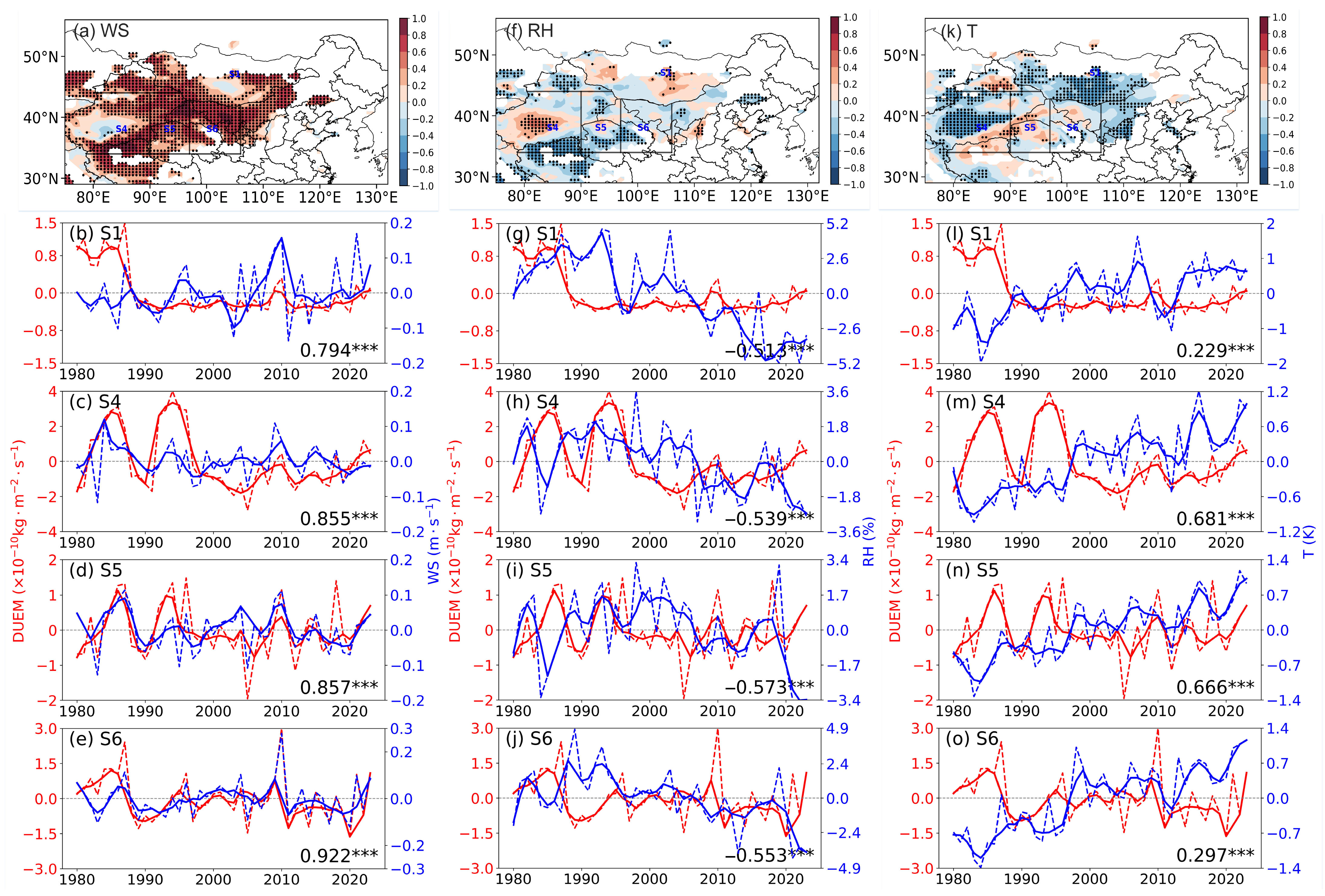
3.3.2. Near-Surface Meteorological Factors

This section provides a detailed analysis of the meteorological factors that significantly impact dust emissions, including WS, RH, and T, in four representative regions: S1, S4, S5, and S6. From the distribution of spatial correlation coefficients, WS shows a strong positive correlation with dust emissions in the primary dust source regions of East Asia (Figure 10a), indicating that WS serves as a key driver of dust emissions in these areas. In contrast, RH in regions such as S5 and S6 exhibits a significant negative correlation with dust emissions (Figure 10f). Lower RH levels reduce soil moisture content and weaken surface soil cohesion, thereby intensifying wind erosion and increasing dust emissions. Temperature, on the other hand, demonstrates a notable negative correlation with dust emissions in S1 and S4 (Figure 10k). This negative relationship may result from higher temperatures promoting vegetation growth or enhancing local evaporation, both of which increase surface moisture and suppress dust emissions. However, in S5, temperature is positively correlated with dust emissions, suggesting that rising temperatures accelerate soil moisture evaporation, reduce surface humidity, and indirectly amplify wind erosion, leading to increased dust emissions. Unlike these regions, S6 shows a weaker correlation between temperature and dust emissions, likely due to the dominant influence of other environmental factors on dust emissions in this region.

Time series analysis provides further evidence for the driving roles of WS, RH, and T in dust emissions, as well as their regional variability. The interannual trends of WS and dust emissions are closely aligned (Figure 10b–e). A consistent decline in WS since the 1980s has contributed to reduced dust emissions, while a rebound in WS after 2020 has coincided with a marked increase in dust emissions. These findings highlight the critical role of WS as a major meteorological factor influencing the dynamics of dust emissions. However, the impact of declining WS on dust emissions has not been consistent across all regions. In some areas, such as the primary dust source regions (e.g., S1 and S4 in East Asia), dust emissions are highly sensitive to changes in WS, with the decline in WS significantly suppressing dust emissions. In other regions (e.g., S5 and S6), although WS also shows a downward trend, the reduction in dust emissions is less pronounced, and fluctuations or even increases were observed during certain periods. This may be attributed to differences in regional environmental conditions, such as soil moisture, vegetation cover, and human activities, which might partially offset the suppressive effect of declining WS on dust emissions. Similarly, RH exhibits a clear negative correlation with dust emissions over time (Figure 10g–j). Lower humidity levels facilitate the release of dust by reducing soil moisture, thereby intensifying dust emissions. This relationship is particularly pronounced in S5 (R = −0.573) and S6 (R = −0.553), where high aridity makes these regions more vulnerable to wind erosion. Temperature also shows significant positive correlations with dust emissions over time, particularly in S4 and S5, with correlation coefficients of 0.681 and 0.666, respectively (Figure 10l–o). These results suggest that rising temperatures enhance dust emissions by accelerating soil moisture evaporation, thereby indirectly promoting wind erosion.

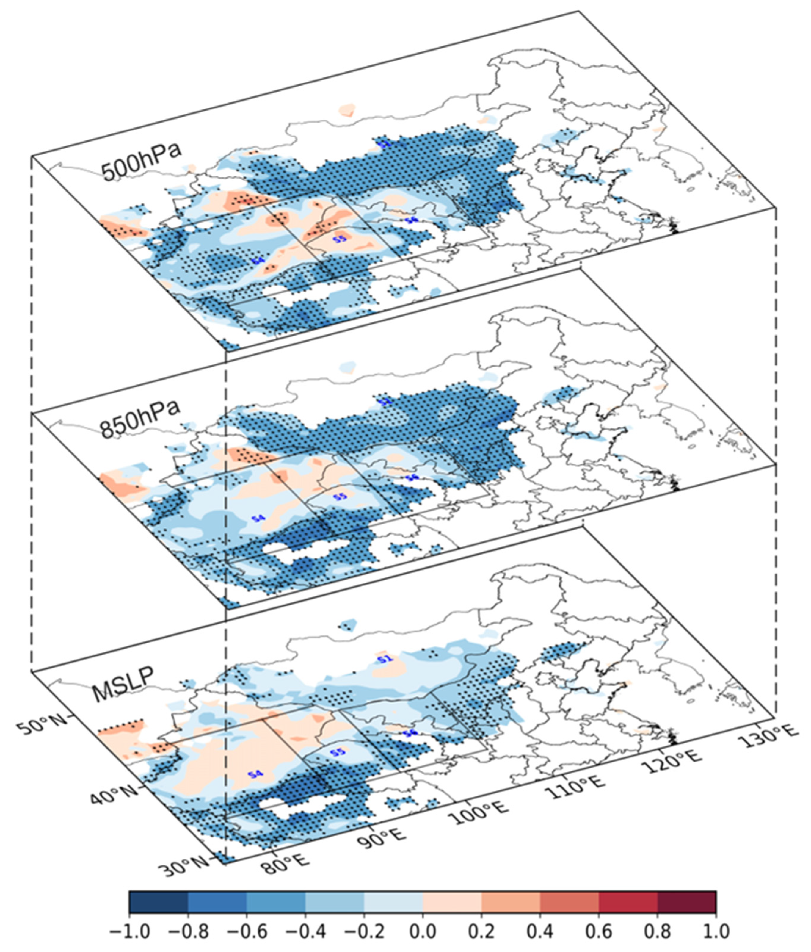
3.3.3. Atmospheric Circulation Patterns

The surface conditions determine the potential dust emission capacity of source areas, while atmospheric circulation factors directly influence dust emissions and long-distance transport by regulating WS, cold air activities, and transport pathways. There is a significant spatial and temporal correlation between DUEM and atmospheric circulation factors, with atmospheric circulation at different levels showing distinct regulatory effects on dust emissions and regional variations (Figure 11). At the 500 hPa level, dust emissions in S1 and parts of northwestern China exhibit a significant negative correlation with GH_500. Lower GH_500 values are often associated with enhanced mid-level cold air activity, which facilitates increased dust emissions. However, in the S4 and S6 regions, the correlation between GH_500 and DUEM is weak, indicating a limited influence of mid-level circulation on dust emissions in these areas. At the 850 hPa level, the correlation is stronger and more widespread, particularly in S4 and S5, where lower-level circulation directly drives dust emissions through increased WS and turbulence. The negative correlation between MSLP and DUEM is most prominent in S4 and S5, suggesting that surface low-pressure systems, such as cyclones, play a critical role in dust emissions in these regions. Detailed time series analysis results are shown in Figure S6, which illustrates the interannual variations between atmospheric circulation factors at different heights (GH_500, GH_850, and MSLP) and dust emission anomalies.

3.3.4. Climate Indices

Table 3. Correlation between dust emissions from different dust sources and climate indices from 1980 to 2023.

Climate Index	S1	S4	S5	S6
AO	−0.576 *** (JFM)	−0.109 (NDJ)	−0.163 (JFM)	−0.567 *** (JFM)
NAO	−0.467 *** (JFM)	0.252 (MAM)	−0.273 * (MAM)	−0.578 *** (JFM)
AAO	−0.419 ** (JFM)	0.268 * (OND)	−0.221 (OND)	−0.344 ** (JFM)
ENSO	0.080 (JFM)	0.244 (MAM)	0.201 (NDJ)	−0.144 (MAM)

Note: *, **, and *** represent the significance test at the 90%, 95%, and 99% levels, respectively.

highlights the periods of maximum correlation between winter-to-spring climate index anomalies and spring dust emission anomalies during 1980–2023. The results show that JFM (January–March) is the most significant period influencing dust emissions. During this time, the AO and NAO exhibit a significant negative correlation with dust emissions in the S1 and S6 regions, with correlation coefficients of −0.576 and −0.567 (AO) and −0.467 and −0.578 (NAO), all reaching the 99% significance level. Similarly, the AAO during JFM also shows a significant negative correlation with dust emissions in S1 and S6, with correlation coefficients of −0.419 and −0.344, respectively, both significant at the 95% level. In contrast, the ENSO shows a generally weaker correlation, only displaying a positive correlation with dust emissions in S4 during MAM (March–May), with a correlation coefficient of 0.244, but this does not reach statistical significance. Therefore, this study primarily focuses on the impact of the AO and NAO on the frequency of dust events during the JFM period.

Figure 12a,d show the spatial correlations between the AO and NAO indices and dust emissions, respectively. Overall, dust emissions in the S1 and S6 regions exhibit significant negative correlations with both the AO and NAO, indicating that their negative phases significantly enhance dust emissions over East Asia. Figure 12b,c present the time series of the AO index and DUEM in the S1 and S6 regions. The correlation coefficients between the AO and DUEM are −0.576 and −0.567, respectively, both passing the 99% significance level. During the negative phase of the AO, polar cold air more easily penetrates southward, leading to frequent strong wind events and dry conditions, which significantly enhance dust emissions. The intensified wind field during the negative phase is one of the primary drivers of dust release and transport. Figure 12e,f display the time series of the NAO index and DUEM in the S1 and S6 regions. Similar to the AO, the NAO also shows significant negative correlations with DUEM, with correlation coefficients of −0.467 and −0.578, respectively. During the negative phase of the NAO, the Siberian High strengthens, and the East Asian trough deepens, leading to more frequent cold air activities and higher surface wind speed, significantly increasing the intensity and frequency of dust emissions. Since the 1980s, dust emissions in S1 and S6 have shown a decreasing trend, while the frequency of positive AO and NAO phases has gradually increased. This suggests that phase variations of the AO and NAO play a crucial role in regulating the intensity and frequency of dust emissions.

4. Discussion

This research systematically analyzes the spatiotemporal variations and driving mechanisms of dust emissions in East Asia from 1980 to 2023. By integrating multi-source data, statistical methods, and SHAP analysis from machine learning, the study reveals significant spatial distribution characteristics and seasonal patterns of dust emissions from major dust source regions in East Asia and identifies key environmental and atmospheric factors affecting dust emissions. Results indicate that dust emissions are primarily driven by meteorological factors, with WS being the most critical influencing factor, while BLH, RH, precipitation, and sea level pressure also significantly impact dust emissions [68,86]. Additionally, regional dust emissions are modulated by the negative phases of the AO and NAO [12,36,87]. Unlike traditional research that mainly relies on statistical analysis and single data sources, this study introduces the SHAP method to quantify complex interactions among various driving factors, providing a new perspective for understanding dust emission mechanisms in East Asia. The research shows that near-surface meteorological factors are the main drivers of dust emissions (contributing 49.4–68.8%), while large-scale climate indices make smaller contributions (2.9–8.0%). Dust emissions typically occur under dry conditions with low pressure, higher BLH, and strong winds, which not only promote dust emissions but also facilitate long-distance transport.

Although this study primarily focuses on dust emissions, regions with high dust emissions do not necessarily experience severe large-scale dust storm events, as dust transport and deposition processes also play critical roles [40,88]. In recent years, dust emissions in Mongolia have increased, although the total emissions remain lower than those of the Taklamakan Desert. However, due to the relatively flat terrain of the Gobi Desert in Mongolia and the increased frequency of southward cold air intrusions induced by climate change, most of the dust is transported downstream along northward and northwestward pathways and achieves long-distance transport under the influence of westerly winds, even reaching more distant regions [40,89,90]. In contrast, the Taklamakan Desert, surrounded by mountains on three sides, has geographic features that are less conducive to the long-range transport of dust particles. Additionally, the region is dominated by easterly winds, which result in less dust being transported downstream. Only when dust is lifted to a certain height and carried by upper-level westerlies can it potentially affect southeastern China. Relevant studies indicate that during dust events in 2023, Mongolia contributed 42% of the dust emissions, while the Taklamakan Desert contributed 26% [83]. The increase in dust emissions in Mongolia and northwestern China is closely related to regional desertification trends. On the one hand, climate change (e.g., reduced precipitation and rising temperatures) may exacerbate surface drying and vegetation degradation, making dust more susceptible to wind transport [91]. On the other hand, land-use changes (e.g., overgrazing, agricultural expansion, and improper water resource management) have also contributed to desertification. Due to the limited implementation of ecological restoration projects in these regions, the effectiveness of such efforts has been relatively weak, resulting in insufficient improvement in vegetation cover and further intensifying desertification in the Mongolian Plateau and western Inner Mongolia [92]. Additionally, in recent years, cold waves and cold air activities have played a significant role in dust emissions in Mongolia and northern China. Extreme cold wave events are often accompanied by intense Mongolian cyclones and cold front activities, which significantly enhance surface WS, facilitating dust transport to northern China and East Asia [93]. Furthermore, anomalous Arctic sea ice changes may also alter the climatic conditions of the Mongolian Plateau and Inner Mongolia by influencing the intensity of the Siberian High and the East Asian winter monsoon [83].

In the early 21st century, China implemented a series of major ecological restoration projects, including the Grain to Green Program (GTGP, 1999), the Beijing–Tianjin Sand Source Control Project (TNSDP, 2001), and the Returning Grazing Land to Grassland Project (RGLGP, 2003) [87]. These policies significantly improved vegetation coverage and reduced the area of bare ground in dust source regions, thereby playing an important role in the downward trend of dust emissions. Based on data analysis from 270 meteorological stations during 1978–2018, Bao et al. [94] found that dust events generally showed a decreasing trend, especially in desert margin areas where significant increases in NDVI indicated improved vegetation coverage [95]. Furthermore, the vegetation improvement trend during 2000–2018 was more pronounced than that during 1982–1999, coinciding with the implementation of ecological restoration policies [96]. These studies suggest that ecological engineering has had significant effects in reducing local dust emissions, improving vegetation cover, and reducing wind erosion [97]. However, due to the complexity of geographical and climatic conditions, spatial distribution differences in dust events remain evident. In regions such as the Taklimakan Desert, NDVI changes were minimal, indicating that ecological engineering has limited impact on long-distance transported dust. Additionally, evaporation and RH remain the main factors affecting dust events [98], suggesting that climatic factors still have important influences on dust emissions. Overall, ecological restoration policies have achieved some success in reducing local dust emissions, particularly with significant vegetation recovery in desert margin areas leading to decreased frequency of dust events. However, due to the influence of cross-regional dust transport and climate change, future research needs to incorporate trajectory analysis and other methods to more accurately assess the long-term effects of ecological engineering.

Although this study did not separately quantify the contribution of human activities to dust emissions, human activities have indirectly influenced dust emissions by altering vegetation coverage, soil moisture, and other factors, which have been incorporated into the analysis of driving factors [99]. It should be clearly pointed out that the correlation analysis between variables and the SHAP method applied in this study are primarily used to explore data patterns and feature importance, but these analyses should not be interpreted as direct evidence of causal relationships. Although the SHAP method can quantify the contribution of features to model predictions, similar to correlation analysis, it reflects statistical associations rather than causal mechanisms. As Pearl [100] emphasized, whether correlations or feature importance indicators in machine learning, they merely indicate statistical associations between variables, while causal inference requires more rigorous theoretical frameworks and methodological support. In complex meteorological and surface conditions, the observed feature importance may be influenced by multiple potential factors, including unmeasured confounding variables, common external driving factors, or reverse causality.

Future research could adopt various methods, such as analyzing the variation characteristics of regional PM_2.5/PM₁₀ ratios, determining the thresholds of background PM₁₀ and PM₁₀ during dust events, and applying source apportionment models to more accurately distinguish the contributions of natural and anthropogenic dust sources [101,102,103,104], as well as implementing causal inference methods such as structural equation modeling, natural experimental designs, or causal graph analysis to more rigorously test hypothesized causal relationships [105,106], which would transcend the limitations of correlation and SHAP analyses presented in this study and more accurately distinguish between feature importance and true causal effects. Additionally, studies could integrate ground-based observations, CALIPSO satellite data, and the HYSPLIT model to further analyze the height and trajectory of dust transport following emissions, thereby elucidating the long-range transport processes of typical recent strong dust events and their impacts on downstream regions [107,108,109]. Furthermore, research should focus on the interaction between natural and anthropogenic factors, particularly regarding regional differences in dust emission mechanisms under the context of climate warming. In regions where human activities have a significant impact, such distinctions and insights would support governments and relevant agencies in formulating more targeted measures to address dust storm disasters, enhance disaster prevention and mitigation capabilities, and provide scientific evidence for ecological and environmental protection.

5. Conclusions

This study systematically analyzed the spatiotemporal characteristics and driving factors of dust emissions in East Asia from 1980 to 2023 using multi-source data. The main conclusions are as follows:

(1)

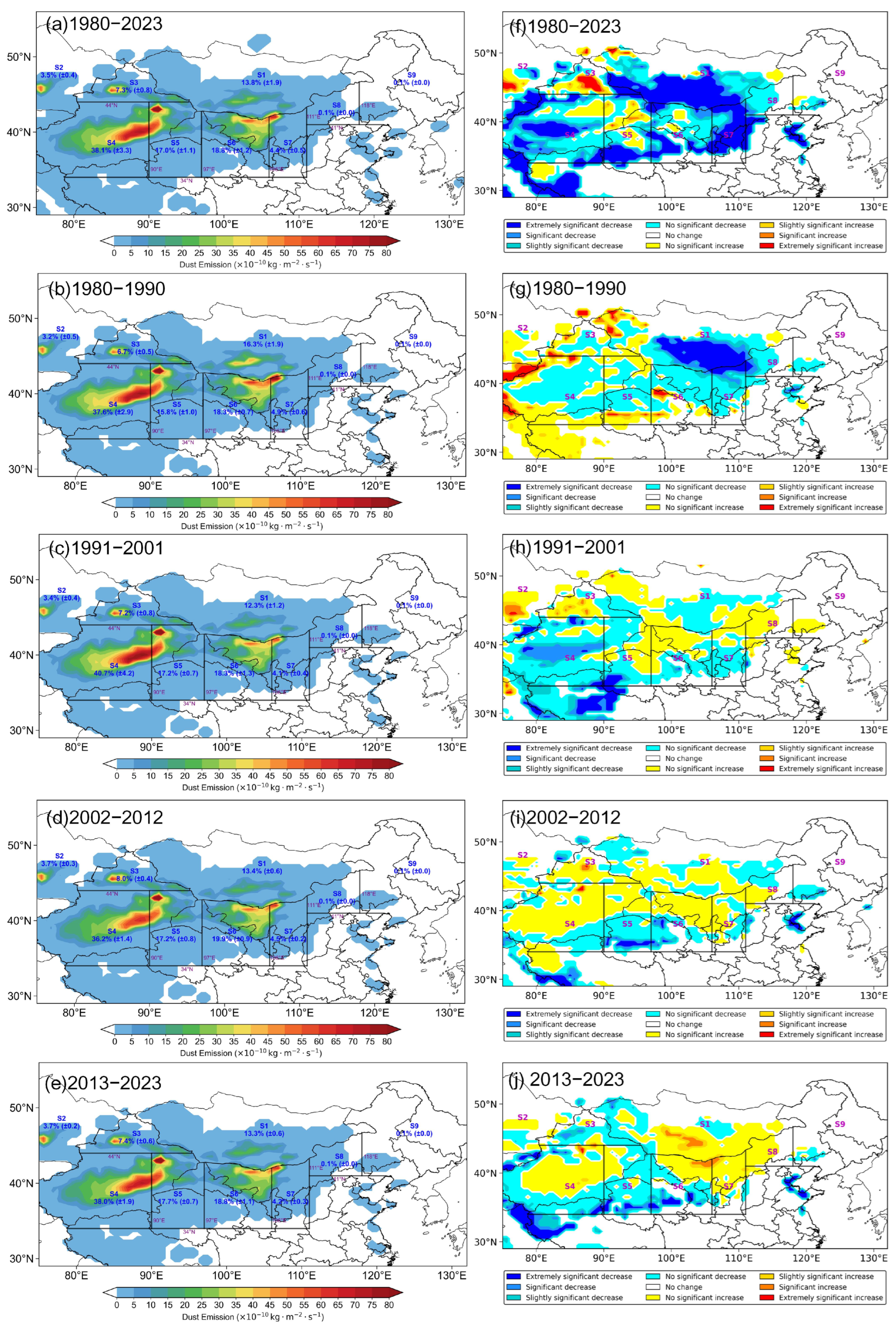
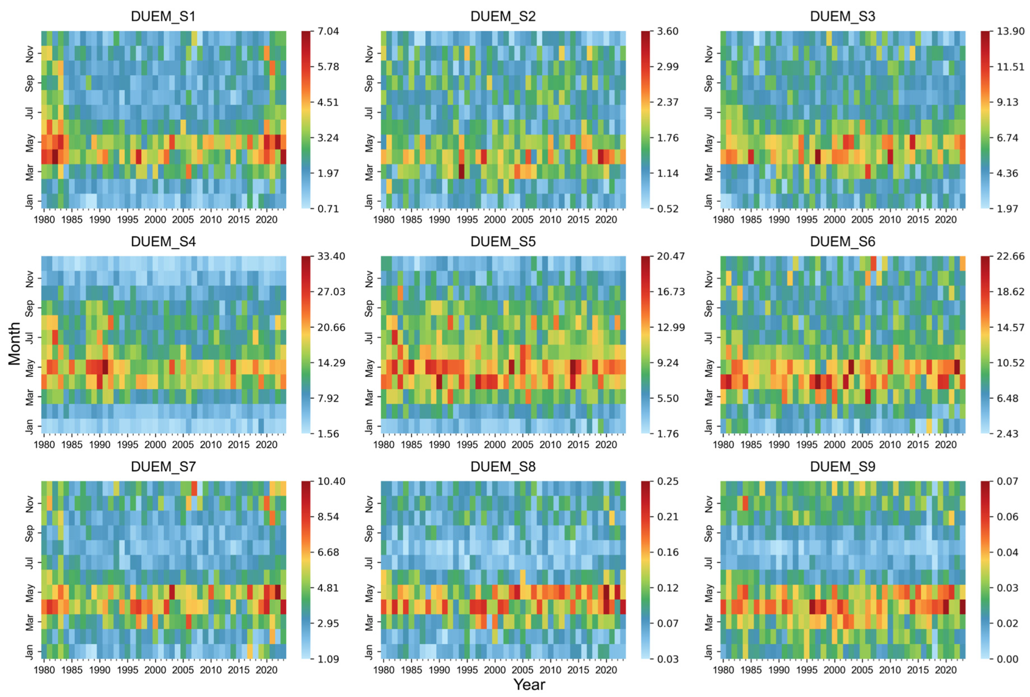
From 1980 to 2023, dust emissions in East Asia exhibited significant spatial and seasonal variations, primarily concentrated in the S1, S4, S5, and S6 regions. Among these, S4 was the strongest dust source, with an average contribution rate of 38.1%, peaking at 40.7% during 1991–2001. S5 and S6 followed, contributing 17.0% and 18.8%, respectively. Outside of China, Mongolia (S1) was the most important dust source, with an average contribution rate of 13.8%. Seasonally, dust emissions in East Asia increased significantly in spring, peaking in April, while remaining at lower levels during winter. In terms of trends, dust emissions generally showed a declining trend from 1980 to 2001. Between 2001 and 2012, the decline slowed, and emissions increased in some areas. From 2012 to 2023, dust emissions in the S1 region rose significantly.

(2)

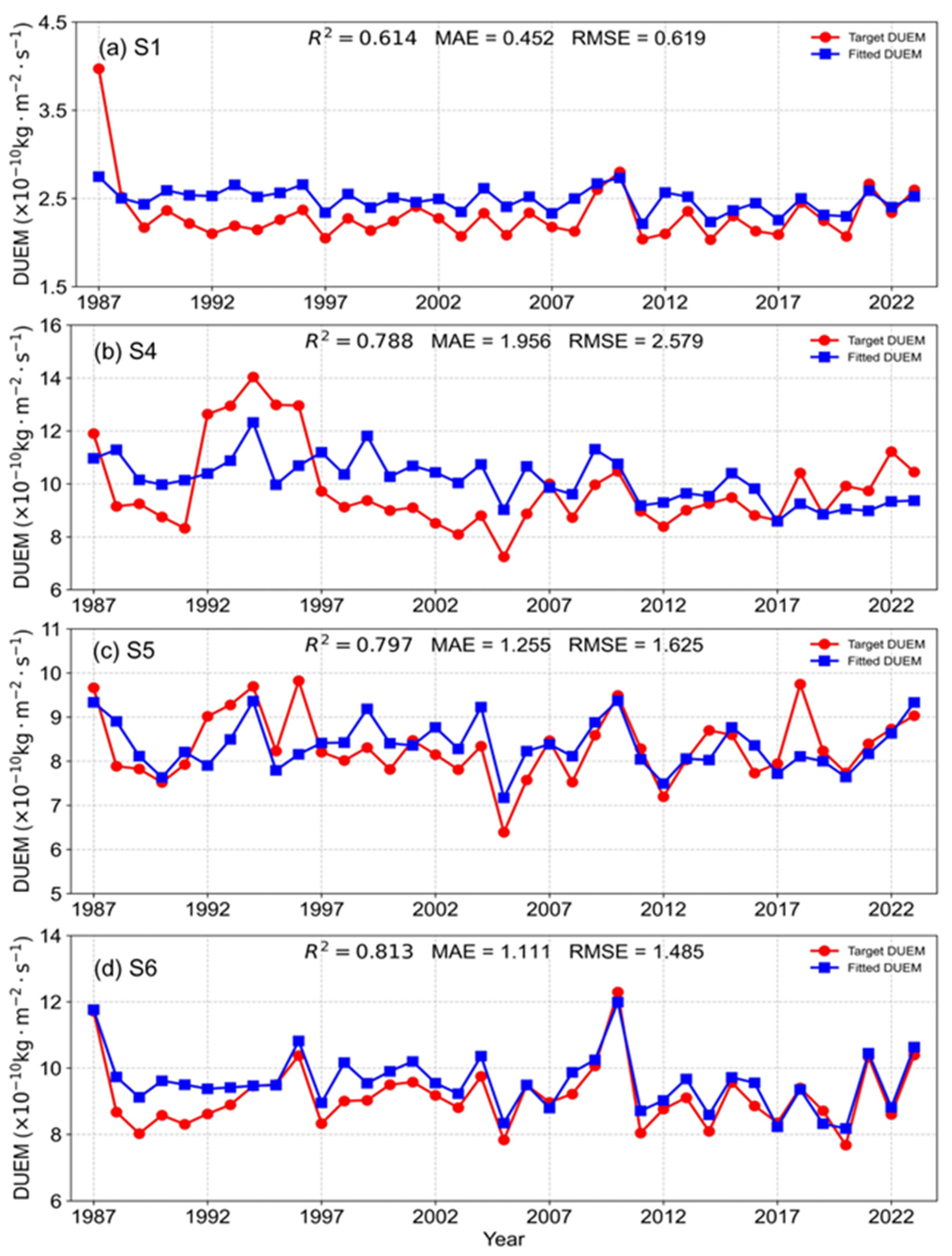
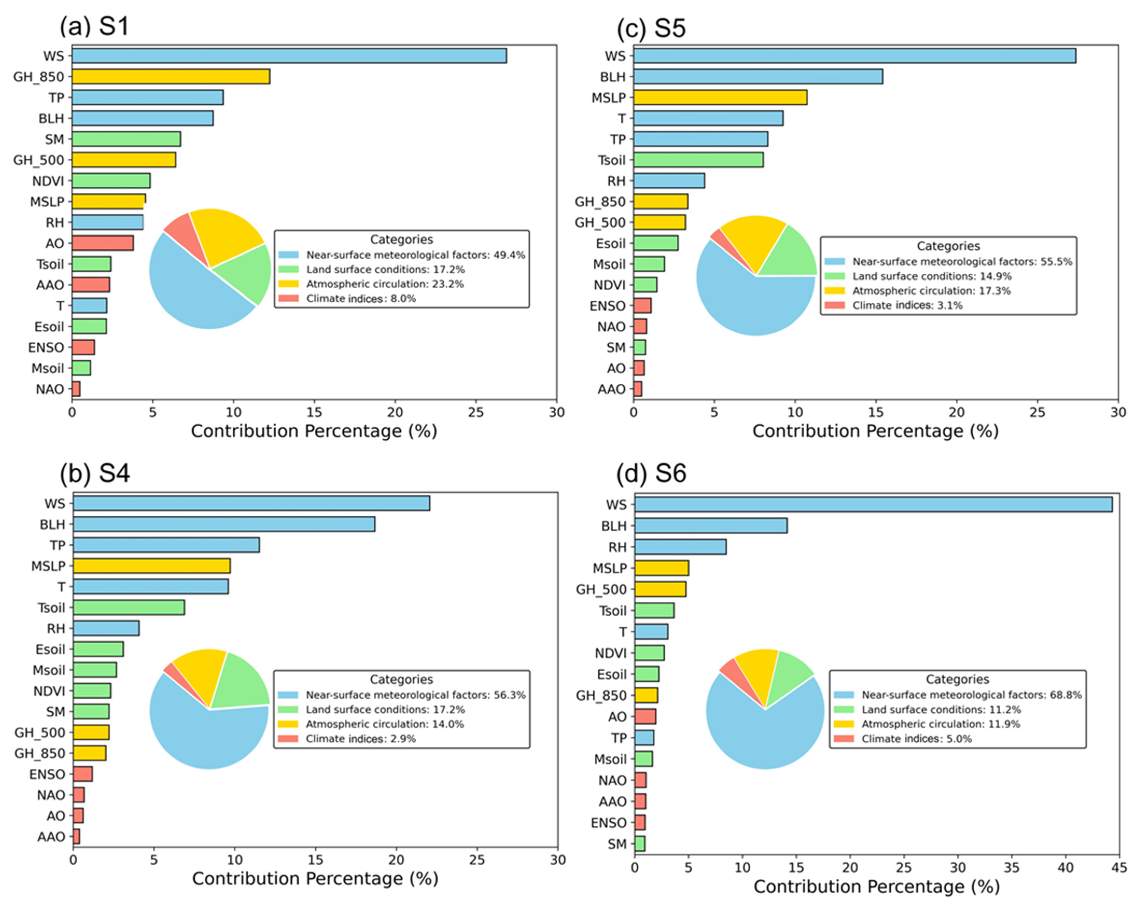
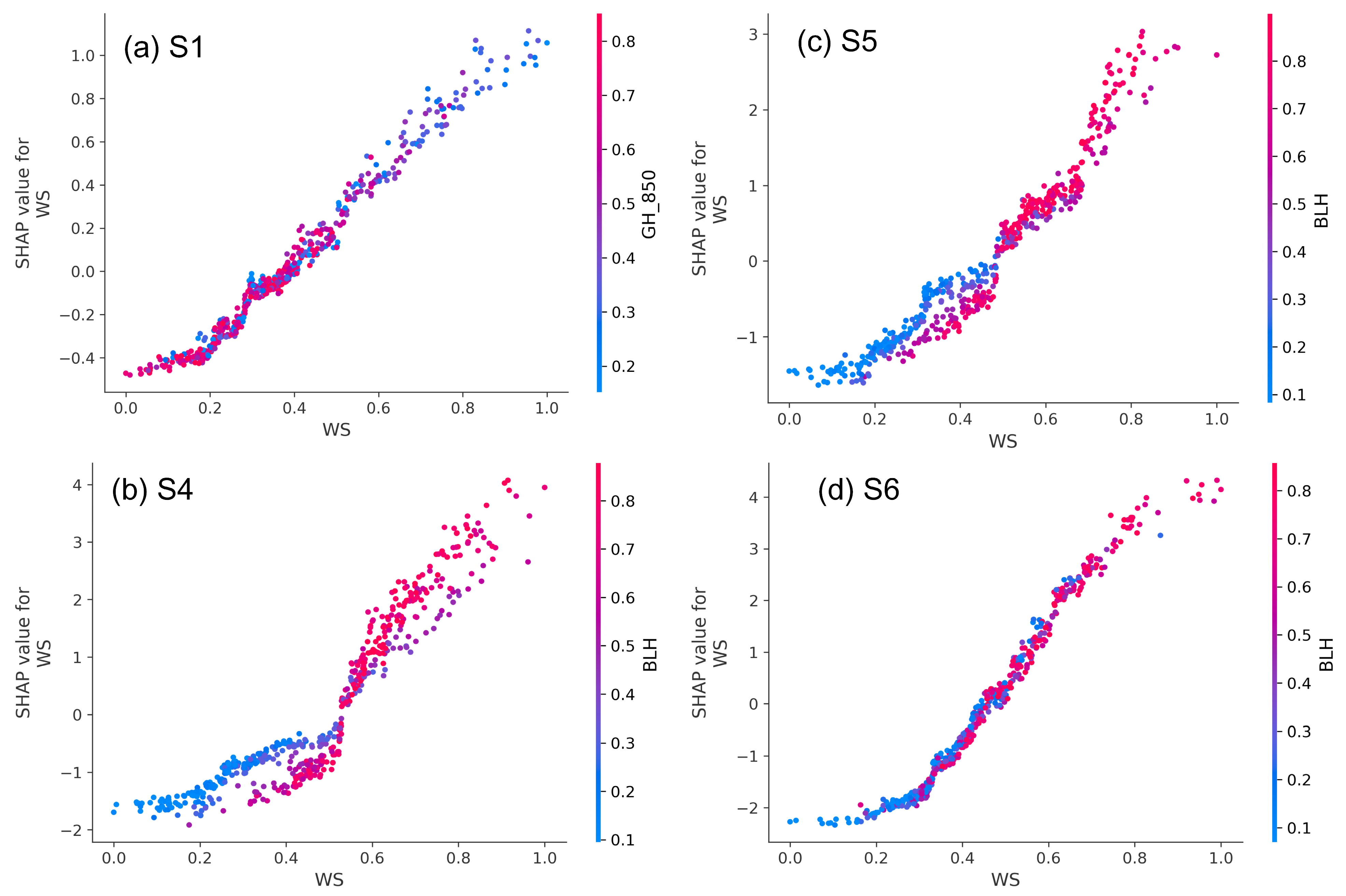
SHAP analysis indicates that near-surface meteorological factors are the primary drivers of dust emissions (contributing 49.4–68.8%), with WS and BLH being the most critical factors. The impact of WS is significant across all regions but is modulated by other factors; low BLH enhances the driving effect of WS, while high BLH weakens it. There are notable regional and seasonal differences in driving factors: in the S1 region, atmospheric circulation (e.g., GH_850) dominates in summer, while near-surface meteorological factors prevail in winter and spring; in the S4 region, local meteorological conditions dominate year-round with minimal seasonal variation; in the S5 and S6 regions, WS and BLH are the main drivers, but the influence of atmospheric circulation increases during summer. These findings reveal the regional, seasonal, and complex mechanisms driving dust emissions.

(3)

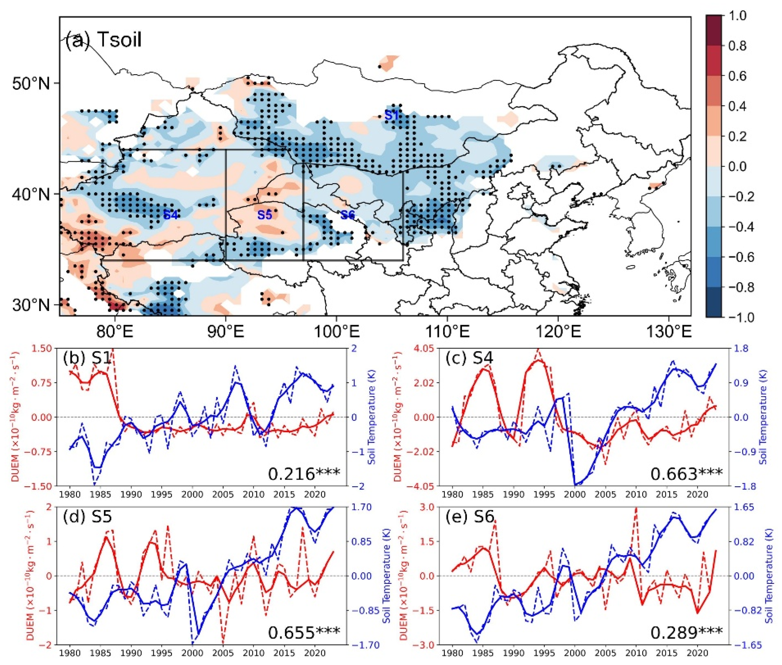
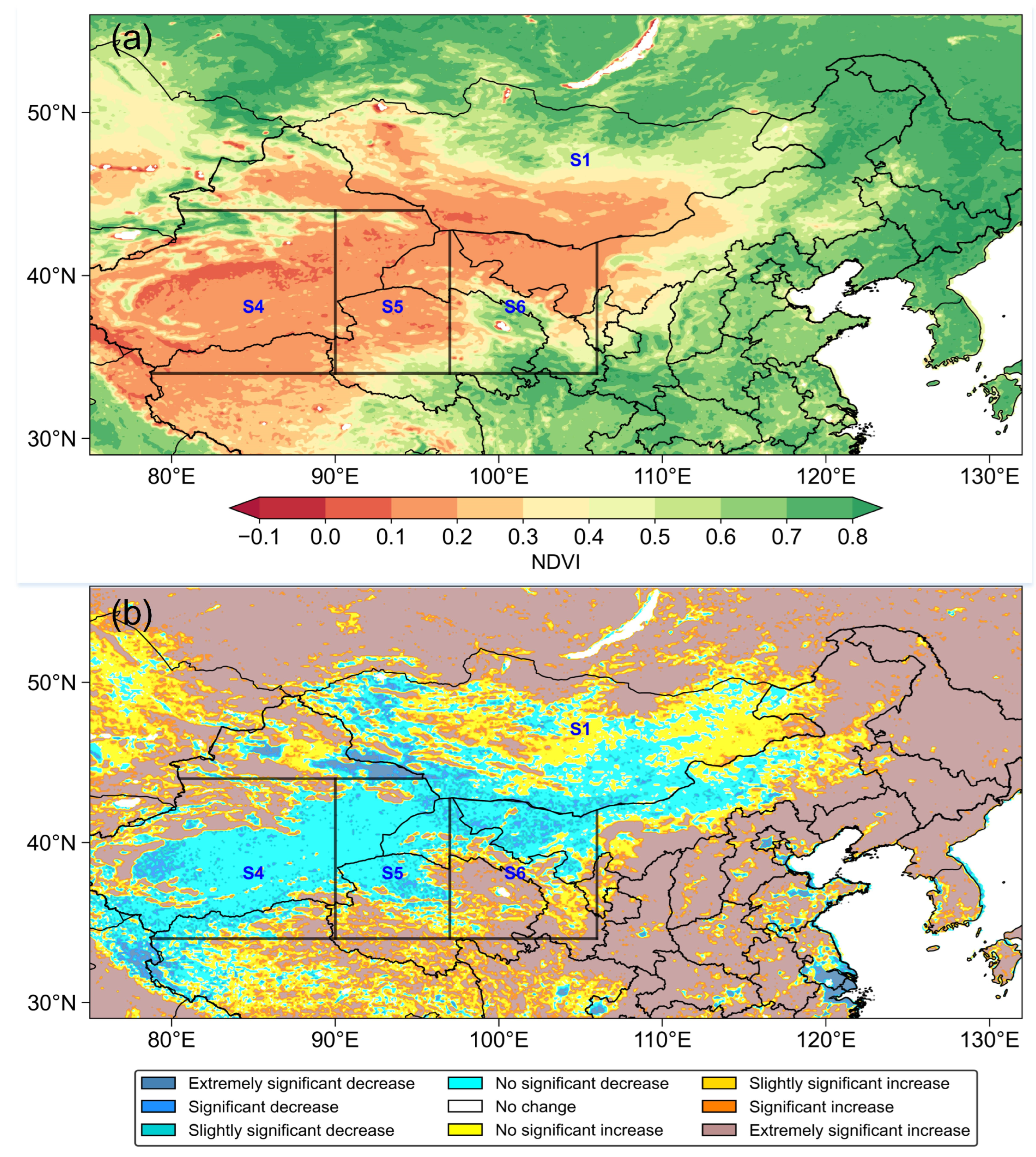
Based on interannual variations and correlation analysis, WS is identified as the primary influencing factor for dust emissions across all regions. RH shows a significant negative correlation with dust emissions in the S5 and S6 regions, indicating that lower humidity conditions are more conducive to dust activity. Among surface conditions, SM has the most significant impact in the S4 and S5 regions, with correlation coefficients of 0.719 and 0.508, respectively. Tsoil also exerts a notable influence in the S4 region (R = 0.663) but has a weaker effect in the S6 region (R = 0.289). Regarding atmospheric circulation, MSLP exhibits the strongest negative correlation with dust emissions in the S4 and S5 regions (R = −0.727 and R = −0.714), suggesting that cyclonic activity significantly enhances wind erosion. Additionally, the negative phases of the AO and NAO significantly promote dust emissions in the S1 and S6 regions by intensifying cold air activity and wind speed, with correlation coefficients of −0.576 and −0.578, respectively.

This study highlights the innovation and practicality of SHAP analysis in interpreting the driving factors of dust emissions. Combined with traditional statistical methods, it provides a more detailed and interpretable approach to understanding the spatiotemporal variations and interactions of key factors. Furthermore, these insights can inform climate mitigation strategies by identifying key regions and periods for targeted interventions, such as afforestation, soil stabilization, and water resource management, to reduce dust emissions and their adverse impacts on regional and global climates.

References

1. Song, H.; Wang, K.; Zhang, Y.; Hong, C.; Zhou, S. Simulation and Evaluation of Dust Emissions with WRF-Chem (v3.7.1) and Its Relationship to the Changing Climate over East Asia from 1980 to 2015. Atmos. Environ. 2017, 167, 511–522. [Google Scholar] [CrossRef]
2. Shao, Y.; Wyrwoll, K.-H.; Chappell, A.; Huang, J.; Lin, Z.; McTainsh, G.H.; Mikami, M.; Tanaka, T.Y.; Wang, X.; Yoon, S. Dust Cycle: An Emerging Core Theme in Earth System Science. Aeolian Res. 2011, 2, 181–204. [Google Scholar] [CrossRef]
3. Liu, X.; Song, H.; Lei, T.; Liu, P.; Xu, C.; Wang, D.; Yang, Z.; Xia, H.; Wang, T.; Zhao, H. Effects of Natural and Anthropogenic Factors and Their Interactions on Dust Events in Northern China. CATENA 2021, 196, 104919. [Google Scholar] [CrossRef]
4. Perlwitz, J.; Tegen, I.; Miller, R.L. Interactive Soil Dust Aerosol Model in the GISS GCM: 1. Sensitivity of the Soil Dust Cycle to Radiative Properties of Soil Dust Aerosols. J. Geophys. Res. Atmos. 2001, 106, 18167–18192. [Google Scholar] [CrossRef]
5. Sokolik, I.N.; Toon, O.B.; Bergstrom, R.W. Modeling the Radiative Characteristics of Airborne Mineral Aerosols at Infrared Wavelengths. J. Geophys. Res. Atmos. 1998, 103, 8813–8826. [Google Scholar] [CrossRef]
6. Miller, R.L.; Tegen, I. Climate Response to Soil Dust Aerosols. J. Clim. 1998, 11, 3247–3267. [Google Scholar] [CrossRef]
7. Liao, H.; Seinfeld, J.H. Radiative Forcing by Mineral Dust Aerosols: Sensitivity to Key Variables. J. Geophys. Res. Atmos. 1998, 103, 31637–31645. [Google Scholar] [CrossRef]
8. Creamean, J.M.; Suski, K.J.; Rosenfeld, D.; Cazorla, A.; DeMott, P.J.; Sullivan, R.C.; White, A.B.; Ralph, F.M.; Minnis, P.; Comstock, J.M.; et al. Dust and Biological Aerosols from the Sahara and Asia Influence Precipitation in the Western U.S. Science 2013, 339, 1572–1578. [Google Scholar] [CrossRef]
9. Singh, R.P.; Prasad, A.K.; Kayetha, V.K.; Kafatos, M. Enhancement of Oceanic Parameters Associated with Dust Storms Using Satellite Data. J. Geophys. Res. Oceans 2008, 113, 2008JC004815. [Google Scholar] [CrossRef]
10. Zhang, X.Y.; Gong, S.L.; Zhao, T.L.; Arimoto, R.; Wang, Y.Q.; Zhou, Z.J. Sources of Asian Dust and Role of Climate Change versus Desertification in Asian Dust Emission. Geophys. Res. Lett. 2003, 30, 2003GL018206. [Google Scholar] [CrossRef]
11. Middleton, N.J. Desert Dust Hazards: A Global Review. Aeolian Res. 2017, 24, 53–63. [Google Scholar] [CrossRef]
12. Wang, N.; Chen, J.; Zhang, Y.; Xu, Y.; Yu, W. The Spatiotemporal Characteristics and Driving Factors of Dust Emissions in East Asia (2000–2021). Remote Sens. 2023, 15, 410. [Google Scholar] [CrossRef]
13. Filonchyk, M.; Peterson, M.P.; Zhang, L.; Yan, H. An Analysis of Air Pollution Associated with the 2023 Sand and Dust Storms over China: Aerosol Properties and PM10 Variability. Geosci. Front. 2024, 15, 101762. [Google Scholar] [CrossRef]
14. Aili, A.; Xu, H.; Kasim, T.; Abulikemu, A. Origin and Transport Pathway of Dust Storm and Its Contribution to Particulate Air Pollution in Northeast Edge of Taklimakan Desert, China. Atmosphere 2021, 12, 113. [Google Scholar] [CrossRef]
15. Wang, X.; Liu, J.; Che, H.; Ji, F.; Liu, J. Spatial and Temporal Evolution of Natural and Anthropogenic Dust Events over Northern China. Sci. Rep. 2018, 8, 2141. [Google Scholar] [CrossRef]
16. Wu, C.; Lin, Z.; Liu, X.; Li, Y.; Lu, Z.; Wu, M. Can Climate Models Reproduce the Decadal Change of Dust Aerosol in East Asia? Geophys. Res. Lett. 2018, 45, 9953–9962. [Google Scholar] [CrossRef]
17. Shao, Y.; Klose, M.; Wyrwoll, K. Recent Global Dust Trend and Connections to Climate Forcing. J. Geophys. Res. Atmos. 2013, 118, 11107–11118. [Google Scholar] [CrossRef]
18. Ginoux, P.; Prospero, J.M.; Gill, T.E.; Hsu, N.C.; Zhao, M. Global-scale Attribution of Anthropogenic and Natural Dust Sources and Their Emission Rates Based on MODIS Deep Blue Aerosol Products. Rev. Geophys. 2012, 50, 2012RG000388. [Google Scholar] [CrossRef]
19. Huang, J.; Wang, T.; Wang, W.; Li, Z.; Yan, H. Climate Effects of Dust Aerosols over East Asian Arid and Semiarid Regions. J. Geophys. Res. Atmos. 2014, 119, 11398–11416. [Google Scholar] [CrossRef]
20. Kok, J.F.; Ridley, D.A.; Zhou, Q.; Miller, R.L.; Zhao, C.; Heald, C.L.; Ward, D.S.; Albani, S.; Haustein, K. Smaller Desert Dust Cooling Effect Estimated from Analysis of Dust Size and Abundance. Nat. Geosci. 2017, 10, 274–278. [Google Scholar] [CrossRef]
21. An, L.; Che, H.; Xue, M.; Zhang, T.; Wang, H.; Wang, Y.; Zhou, C.; Zhao, H.; Gui, K.; Zheng, Y.; et al. Temporal and Spatial Variations in Sand and Dust Storm Events in East Asia from 2007 to 2016: Relationships with Surface Conditions and Climate Change. Sci. Total Environ. 2018, 633, 452–462. [Google Scholar] [CrossRef]
22. Pu, W.; Wang, X.; Zhang, X.; Ren, Y.; Shi, J.-S.; Bi, J.-R.; Zhang, B.-D. Size Distribution and Optical Properties of Particulate Matter (PM10) and Black Carbon (BC) during Dust Storms and Local Air Pollution Events across a Loess Plateau Site. Aerosol Air Qual. Res. 2015, 15, 2212–2224. [Google Scholar] [CrossRef]
23. Yang, Y.; Russell, L.M.; Lou, S.; Liao, H.; Guo, J.; Liu, Y.; Singh, B.; Ghan, S.J. Dust-Wind Interactions Can Intensify Aerosol Pollution over Eastern China. Nat. Commun. 2017, 8, 15333. [Google Scholar] [CrossRef] [PubMed]
24. Liu, X.; Yin, Z.; Zhang, X.; Yang, X. Analyses of the Spring Dust Storm Frequency of Northern China in Relation to Antecedent and Concurrent Wind, Precipitation, Vegetation, and Soil Moisture Conditions. J. Geophys. Res. Atmos. 2004, 109, 2004JD004615. [Google Scholar] [CrossRef]
25. Munkhtsetseg, E.; Shinoda, M.; Gillies, J.A.; Kimura, R.; King, J.; Nikolich, G. Relationships between Soil Moisture and Dust Emissions in a Bare Sandy Soil of Mongolia. Particuology 2016, 28, 131–137. [Google Scholar] [CrossRef]
26. Yin, Z.; Wan, Y.; Zhang, Y.; Wang, H. Why Super Sandstorm 2021 in North China? Natl. Sci. Rev. 2022, 9, nwab165. [Google Scholar] [CrossRef] [PubMed]
27. Zou, X.K.; Zhai, P.M. Relationship between Vegetation Coverage and Spring Dust Storms over Northern China. J. Geophys. Res. Atmos. 2004, 109, 2003JD003913. [Google Scholar] [CrossRef]
28. Abulaiti, A.; Kimura, R.; Shinoda, M.; Kurosaki, Y.; Mikami, M.; Ishizuka, M.; Yamada, Y.; Nishihara, E.; Gantsetseg, B. An Observational Study of Saltation and Dust Emission in a Hotspot of Mongolia. Aeolian Res. 2014, 15, 169–176. [Google Scholar] [CrossRef]
29. Xu, C. Spatiotemporal Variations and Driving Factors of Dust Storm Events in Northern China Based on High-Temporal-Resolution Analysis of Meteorological Data (1960-2007). Environ. Pollut. 2020, 260, 114084. [Google Scholar] [CrossRef]
30. Guo, J.; Lou, M.; Miao, Y.; Wang, Y.; Zeng, Z.; Liu, H.; He, J.; Xu, H.; Wang, F.; Min, M.; et al. Trans-Pacific Transport of Dust Aerosols from East Asia: Insights Gained from Multiple Observations and Modeling. Environ. Pollut. 2017, 230, 1030–1039. [Google Scholar] [CrossRef]
31. Kaskaoutis, D.G.; Houssos, E.E.; Solmon, F.; Legrand, M.; Rashki, A.; Dumka, U.C.; Francois, P.; Gautam, R.; Singh, R.P. Impact of Atmospheric Circulation Types on Southwest Asian Dust and Indian Summer Monsoon Rainfall. Atmos. Res. 2018, 201, 189–205. [Google Scholar] [CrossRef]
32. Mao, R.; Gong, D.; Bao, J.; Fan, Y. Possible Influence of Arctic Oscillation on Dust Storm Frequency in North China. J. Geogr. Sci. 2011, 21, 207–218. [Google Scholar] [CrossRef]
33. Gong, S.L.; Zhang, X.Y.; Zhao, T.L.; Zhang, X.B.; Barrie, L.A.; McKendry, I.G.; Zhao, C.S. A Simulated Climatology of Asian Dust Aerosol and Its Trans-Pacific Transport. Part II: Interannual Variability and Climate Connections. J. Clim. 2006, 19, 104–122. [Google Scholar] [CrossRef]
34. Fan, K.; Wang, H. Dust Storms in North China in 2002: A Case Study of the Low Frequency Oscillation. Adv. Atmos. Sci. 2007, 24, 15–23. [Google Scholar] [CrossRef]
35. Yang, Y.; Zeng, L.; Wang, H.; Wang, P.; Liao, H. Dust Pollution in China Affected by Different Spatial and Temporal Types of El Niño. Atmos. Chem. Phys. 2022, 22, 14489–14502. [Google Scholar] [CrossRef]
36. Xu, F.; Wang, S.; Li, Y.; Feng, J. Synergistic Effects of the Winter North Atlantic Oscillation (NAO) and El Niño–Southern Oscillation (ENSO) on Dust Activities in North China during the Following Spring. Atmos. Chem. Phys. 2024, 24, 10689–10705. [Google Scholar] [CrossRef]
37. Grell, G.A.; Peckham, S.E.; Schmitz, R.; McKeen, S.A.; Frost, G.; Skamarock, W.C.; Eder, B. Fully Coupled “Online” Chemistry within the WRF Model. Atmos. Environ. 2005, 39, 6957–6975. [Google Scholar] [CrossRef]
38. Giorgi, F.; Coppola, E.; Solmon, F.; Mariotti, L.; Sylla, M.; Bi, X.; Elguindi, N.; Diro, G.; Nair, V.; Giuliani, G.; et al. RegCM4: Model Description and Preliminary Tests over Multiple CORDEX Domains. Clim. Res. 2012, 52, 7–29. [Google Scholar] [CrossRef]
39. Nickovic, S.; Kallos, G.; Papadopoulos, A.; Kakaliagou, O. A Model for Prediction of Desert Dust Cycle in the Atmosphere. J. Geophys. Res. Atmos. 2001, 106, 18113–18129. [Google Scholar] [CrossRef]
40. Huang, J.; Minnis, P.; Chen, B.; Huang, Z.; Liu, Z.; Zhao, Q.; Yi, Y.; Ayers, J.K. Long-range Transport and Vertical Structure of Asian Dust from CALIPSO and Surface Measurements during PACDEX. J. Geophys. Res. Atmos. 2008, 113, 2008JD010620. [Google Scholar] [CrossRef]
41. Kok, J.F.; Mahowald, N.M.; Fratini, G.; Gillies, J.A.; Ishizuka, M.; Leys, J.F.; Mikami, M.; Park, M.-S.; Park, S.-U.; Van Pelt, R.S.; et al. An Improved Dust Emission Model—Part 1: Model Description and Comparison against Measurements. Atmos. Chem. Phys. 2014, 14, 13023–13041. [Google Scholar] [CrossRef]
42. Shao, Y.; Ishizuka, M.; Mikami, M.; Leys, J.F. Parameterization of Size-resolved Dust Emission and Validation with Measurements. J. Geophys. Res. 2011, 116, D08203. [Google Scholar] [CrossRef]
43. Randles, C.A.; Da Silva, A.M.; Buchard, V.; Colarco, P.R.; Darmenov, A.; Govindaraju, R.; Smirnov, A.; Holben, B.; Ferrare, R.; Hair, J.; et al. The MERRA-2 Aerosol Reanalysis, 1980 Onward. Part I: System Description and Data Assimilation Evaluation. J. Clim. 2017, 30, 6823–6850. [Google Scholar] [CrossRef] [PubMed]
44. Gelaro, R.; McCarty, W.; Suárez, M.J.; Todling, R.; Molod, A.; Takacs, L.; Randles, C.A.; Darmenov, A.; Bosilovich, M.G.; Reichle, R.; et al. The Modern-Era Retrospective Analysis for Research and Applications, Version 2 (MERRA-2). J. Clim. 2017, 30, 5419–5454. [Google Scholar] [CrossRef]
45. Shapley, L.S. 17. A Value for n-Person Games. In Contributions to the Theory of Games (AM-28), Volume II; Kuhn, H.W., Tucker, A.W., Eds.; Princeton University Press: Princeton, NJ, USA, 1953; pp. 307–318. ISBN 978-1-4008-8197-0. [Google Scholar]
46. Lundberg, S.M.; Erion, G.; Chen, H.; DeGrave, A.; Prutkin, J.M.; Nair, B.; Katz, R.; Himmelfarb, J.; Bansal, N.; Lee, S.-I. From Local Explanations to Global Understanding with Explainable AI for Trees. Nat. Mach. Intell. 2020, 2, 56–67. [Google Scholar] [CrossRef]
47. Gholami, H.; Jalali, M.; Rezaei, M.; Mohamadifar, A.; Song, Y.; Li, Y.; Wang, Y.; Niu, B.; Omidvar, E.; Kaskaoutis, D.G. An Explainable Integrated Machine Learning Model for Mapping Soil Erosion by Wind and Water in a Catchment with Three Desiccated Lakes. Aeolian Res. 2024, 67–69, 100924. [Google Scholar] [CrossRef]
48. Chen, J.; Cao, X.; Peng, S.; Ren, H. Analysis and Applications of GlobeLand30: A Review. ISPRS Int. J. Geo-Inf. 2017, 6, 230. [Google Scholar] [CrossRef]
49. Chen, J.; Ban, Y.; Li, S. Open Access to Earth Land-Cover Map. Nature 2014, 514, 434. [Google Scholar] [CrossRef]
50. Franch, B.; Vermote, E.; Roger, J.-C.; Murphy, E.; Becker-Reshef, I.; Justice, C.; Claverie, M.; Nagol, J.; Csiszar, I.; Meyer, D.; et al. A 30+ Year AVHRR Land Surface Reflectance Climate Data Record and Its Application to Wheat Yield Monitoring. Remote Sens. 2017, 9, 296. [Google Scholar] [CrossRef]
51. Huang, S.; Tang, L.; Hupy, J.P.; Wang, Y.; Shao, G. A Commentary Review on the Use of Normalized Difference Vegetation Index (NDVI) in the Era of Popular Remote Sensing. J. For. Res. 2021, 32, 1–6. [Google Scholar] [CrossRef]
52. Buchard, V.; Randles, C.A.; Da Silva, A.M.; Darmenov, A.; Colarco, P.R.; Govindaraju, R.; Ferrare, R.; Hair, J.; Beyersdorf, A.J.; Ziemba, L.D.; et al. The MERRA-2 Aerosol Reanalysis, 1980 Onward. Part II: Evaluation and Case Studies. J. Clim. 2017, 30, 6851–6872. [Google Scholar] [CrossRef] [PubMed]
53. Diner, D.J.; Bruegge, C.J.; Martonchik, J.V.; Ackerman, T.P.; Davies, R.; Gerstl, S.A.W.; Gordon, H.R.; Sellers, P.J.; Clark, J.; Daniels, J.A.; et al. MISR: A Multiangle Imaging Spectroradiometer for Geophysical and Climatological Research from Eos. IEEE Trans. Geosci. Remote Sens. 1989, 27, 200–214. [Google Scholar] [CrossRef]
54. Dubovik, O.; Smirnov, A.; Holben, B.N.; King, M.D.; Kaufman, Y.J.; Eck, T.F.; Slutsker, I. Accuracy Assessments of Aerosol Optical Properties Retrieved from Aerosol Robotic Network (AERONET) Sun and Sky Radiance Measurements. J. Geophys. Res. Atmos. 2000, 105, 9791–9806. [Google Scholar] [CrossRef]
55. Shi, L.; Zhang, J.; Yao, F.; Zhang, D.; Guo, H. Temporal Variation of Dust Emissions in Dust Sources over Central Asia in Recent Decades and the Climate Linkages. Atmos. Environ. 2020, 222, 117176. [Google Scholar] [CrossRef]
56. Ginoux, P.; Chin, M.; Tegen, I.; Prospero, J.M.; Holben, B.; Dubovik, O.; Lin, S. Sources and Distributions of Dust Aerosols Simulated with the GOCART Model. J. Geophys. Res. Atmos. 2001, 106, 20255–20273. [Google Scholar] [CrossRef]
57. Jing, Y.; Zhang, P.; Chen, L.; Xu, N. Integrated Analysis of Dust Transport and Budget in a Severe Asian Dust Event. Aerosol Air Qual. Res. 2017, 17, 2390–2400. [Google Scholar] [CrossRef]
58. Yao, W.; Che, H.; Gui, K.; Wang, Y.; Zhang, X. Can MERRA-2 Reanalysis Data Reproduce the Three-Dimensional Evolution Characteristics of a Typical Dust Process in East Asia? A Case Study of the Dust Event in May 2017. Remote Sens. 2020, 12, 902. [Google Scholar] [CrossRef]
59. Shi, L.; Zhang, J.; Yao, F.; Zhang, D.; Guo, H. Drivers to Dust Emissions over Dust Belt from 1980 to 2018 and Their Variation in Two Global Warming Phases. Sci. Total Environ. 2021, 767, 144860. [Google Scholar] [CrossRef]
60. Chen, Y.; Yang, K.; Qin, J.; Zhao, L.; Tang, W.; Han, M. Evaluation of AMSR-E Retrievals and GLDAS Simulations against Observations of a Soil Moisture Network on the Central Tibetan Plateau. J. Geophys. Res. Atmos. 2013, 118, 4466–4475. [Google Scholar] [CrossRef]
61. Rodell, M.; Houser, P.R.; Jambor, U.; Gottschalck, J.; Mitchell, K.; Meng, C.-J.; Arsenault, K.; Cosgrove, B.; Radakovich, J.; Bosilovich, M.; et al. The Global Land Data Assimilation System. Bull. Am. Meteorol. Soc. 2004, 85, 381–394. [Google Scholar] [CrossRef]
62. Wang, W.; Cui, W.; Wang, X.; Chen, X. Evaluation of GLDAS-1 and GLDAS-2 Forcing Data and Noah Model Simulations over China at the Monthly Scale. J. Hydrometeorol. 2016, 17, 2815–2833. [Google Scholar] [CrossRef]
63. Hoffmann, L.; Günther, G.; Li, D.; Stein, O.; Wu, X.; Griessbach, S.; Heng, Y.; Konopka, P.; Müller, R.; Vogel, B.; et al. From ERA-Interim to ERA5: The Considerable Impact of ECMWF’s next-Generation Reanalysis on Lagrangian Transport Simulations. Atmos. Chem. Phys. 2019, 19, 3097–3124. [Google Scholar] [CrossRef]
64. Tarek, M.; Brissette, F.P.; Arsenault, R. Evaluation of the ERA5 Reanalysis as a Potential Reference Dataset for Hydrological Modelling over North America. Hydrol. Earth Syst. Sci. 2020, 24, 2527–2544. [Google Scholar] [CrossRef]
65. Hersbach, H.; Bell, B.; Berrisford, P.; Hirahara, S.; Horányi, A.; Muñoz-Sabater, J.; Nicolas, J.; Peubey, C.; Radu, R.; Schepers, D.; et al. The ERA5 Global Reanalysis. Q. J. R. Meteorol. Soc. 2020, 146, 1999–2049. [Google Scholar] [CrossRef]
66. Wang, Y.; Tang, J.; Wang, W.; Wang, Z.; Wang, J.; Liang, S.; Chu, B. Long-Term Spatiotemporal Characteristics and Influencing Factors of Dust Aerosols in East Asia (2000–2022). Remote Sens. 2024, 16, 318. [Google Scholar] [CrossRef]
67. Bai, C.; Cai, Z.; Yin, X.; Zhang, J. LSDSSIMR: Large-Scale Dust Storm Database Based on Satellite Images and Meteorological Reanalysis Data. IEEE J. Sel. Top. Appl. Earth Obs. Remote Sens. 2023, 16, 10121–10131. [Google Scholar] [CrossRef]
68. Gui, K.; Yao, W.; Che, H.; An, L.; Zheng, Y.; Li, L.; Zhao, H.; Zhang, L.; Zhong, J.; Wang, Y.; et al. Record-Breaking Dust Loading during Two Mega Dust Storm Events over Northern China in March 2021: Aerosol Optical and Radiative Properties and Meteorological Drivers. Atmos. Chem. Phys. 2022, 22, 7905–7932. [Google Scholar] [CrossRef]
69. Jiang, Q.; Li, W.; Fan, Z.; He, X.; Sun, W.; Chen, S.; Wen, J.; Gao, J.; Wang, J. Evaluation of the ERA5 Reanalysis Precipitation Dataset over Chinese Mainland. J. Hydrol. 2021, 595, 125660. [Google Scholar] [CrossRef]
70. Dullaart, J.C.M.; Muis, S.; Bloemendaal, N.; Aerts, J.C.J.H. Advancing Global Storm Surge Modelling Using the New ERA5 Climate Reanalysis. Clim. Dyn. 2020, 54, 1007–1021. [Google Scholar] [CrossRef]
71. Kendall, M.G. Rank and Product-Moment Correlation. Biometrika 1949, 36, 177–193. [Google Scholar] [CrossRef]
72. Mann, H.B. Nonparametric Tests against Trend. Econometrica 1945, 13, 245. [Google Scholar] [CrossRef]
73. Gowthaman, T.; Kumar, S.; Bhattacharyya, B. Detecting Air Pollutants Trends Using Mann-Kendall Tests and Sen’s Slope Estimates. Environ. Conserv. J. 2023, 24, 157–166. [Google Scholar] [CrossRef]
74. Li, Y.; Yang, X.; Wang, S.; Cui, S. Insight into Municipal Reactive Nitrogen Emissions and Their Influencing Factors: A Case Study of Xiamen City, China. Atmosphere 2023, 14, 1549. [Google Scholar] [CrossRef]
75. Chen, T.; Guestrin, C. XGBoost: A Scalable Tree Boosting System. In Proceedings of the 22nd ACM SIGKDD International Conference on Knowledge Discovery and Data Mining, San Francisco, CA, USA, 13–17 August 2016; pp. 785–794. [Google Scholar]
76. Toharudin, T.; Caraka, R.E.; Pratiwi, I.R.; Kim, Y.; Gio, P.U.; Sakti, A.D.; Noh, M.; Nugraha, F.A.L.; Pontoh, R.S.; Putri, T.H.; et al. Boosting Algorithm to Handle Unbalanced Classification of PM2.5 Concentration Levels by Observing Meteorological Parameters in Jakarta-Indonesia Using AdaBoost, XGBoost, CatBoost, and LightGBM. IEEE Access 2023, 11, 35680–35696. [Google Scholar] [CrossRef]
77. Mienye, I.D.; Sun, Y. A Survey of Ensemble Learning: Concepts, Algorithms, Applications, and Prospects. IEEE Access 2022, 10, 99129–99149. [Google Scholar] [CrossRef]
78. Štrumbelj, E.; Kononenko, I. Explaining Prediction Models and Individual Predictions with Feature Contributions. Knowl. Inf. Syst. 2014, 41, 647–665. [Google Scholar] [CrossRef]
79. Barredo Arrieta, A.; Díaz-Rodríguez, N.; Del Ser, J.; Bennetot, A.; Tabik, S.; Barbado, A.; Garcia, S.; Gil-Lopez, S.; Molina, D.; Benjamins, R.; et al. Explainable Artificial Intelligence (XAI): Concepts, Taxonomies, Opportunities and Challenges toward Responsible AI. Inf. Fusion 2020, 58, 82–115. [Google Scholar] [CrossRef]
80. Hu, Q.; Moon, J.; Kim, H. Understanding the Driving Forces of Summer PM1 Composition in Seoul, Korea, with Explainable Machine Learning. ACS EST Air 2024, 1, 960–972. [Google Scholar] [CrossRef]
81. Kosaka, Y.; Xie, S.-P. Recent Global-Warming Hiatus Tied to Equatorial Pacific Surface Cooling. Nature 2013, 501, 403–407. [Google Scholar] [CrossRef]
82. Fyfe, J.C.; Gillett, N.P.; Zwiers, F.W. Overestimated Global Warming over the Past 20 Years. Nat. Clim. Change 2013, 3, 767–769. [Google Scholar] [CrossRef]
83. Chen, S.; Zhao, D.; Huang, J.; He, J.; Chen, Y.; Chen, J.; Bi, H.; Lou, G.; Du, S.; Zhang, Y.; et al. Mongolia Contributed More than 42% of the Dust Concentrations in Northern China in March and April 2023. Adv. Atmos. Sci. 2023, 40, 1549–1557. [Google Scholar] [CrossRef]
84. Cleveland, W.S. Robust Locally Weighted Regression and Smoothing Scatterplots. J. Am. Stat. Assoc. 1979, 74, 829–836. [Google Scholar] [CrossRef]
85. Dodig, A.; Ricci, E.; Kvascev, G.; Stojkovic, M. A Novel Machine Learning-Based Framework for the Water Quality Parameters Prediction Using Hybrid Long Short-Term Memory and Locally Weighted Scatterplot Smoothing Methods. J. Hydroinform. 2024, 26, 1059–1079. [Google Scholar] [CrossRef]
86. Yao, W.; Gui, K.; Wang, Y.; Che, H.; Zhang, X. Identifying the Dominant Local Factors of 2000–2019 Changes in Dust Loading over East Asia. Sci. Total Environ. 2021, 777, 146064. [Google Scholar] [CrossRef]
87. Wu, C.; Lin, Z.; Shao, Y.; Liu, X.; Li, Y. Drivers of Recent Decline in Dust Activity over East Asia. Nat. Commun. 2022, 13, 7105. [Google Scholar] [CrossRef]
88. Sun, J.; Zhang, M.; Liu, T. Spatial and Temporal Characteristics of Dust Storms in China and Its Surrounding Regions, 1960–1999: Relations to Source Area and Climate. J. Geophys. Res. Atmos. 2001, 106, 10325–10333. [Google Scholar] [CrossRef]
89. Uno, I.; Eguchi, K.; Yumimoto, K.; Takemura, T.; Shimizu, A.; Uematsu, M.; Liu, Z.; Wang, Z.; Hara, Y.; Sugimoto, N. Asian Dust Transported One Full Circuit around the Globe. Nat. Geosci. 2009, 2, 557–560. [Google Scholar] [CrossRef]
90. Yang, M.; Zhu, X.; Pan, H.; Ai, W.; Song, W.; Pan, Y. Changes of the Relationship between Spring Sand Dust Frequency and Large-Scale Atmospheric Circulation. Atmos. Res. 2019, 226, 102–109. [Google Scholar] [CrossRef]
91. Kimura, R. Factors Contributing to Dust Storms in Source Regions Producing the Yellow-Sand Phenomena Observed in Japan from 1993 to 2002. J. Arid Environ. 2012, 80, 40–44. [Google Scholar] [CrossRef]
92. Han, J.; Dai, H.; Gu, Z. Sandstorms and Desertification in Mongolia, an Example of Future Climate Events: A Review. Environ. Chem. Lett. 2021, 19, 4063–4073. [Google Scholar] [CrossRef]
93. Kim, J. Transport Routes and Source Regions of Asian Dust Observed in Korea during the Past 40 Years (1965–2004). Atmos. Environ. 2008, 42, 4778–4789. [Google Scholar] [CrossRef]
94. Bao, T.; Li, J.; Chang, I.-S.; Jin, E.; Wu, J.; Burenjargal; Bao, Y. The Influence of Ecological Engineering Projects on Dust Events: A Case Study in the Northern China. Environ. Impact Assess. Rev. 2022, 96, 106847. [Google Scholar] [CrossRef]
95. Piao, S.; Wang, X.; Ciais, P.; Zhu, B.; Wang, T.; Liu, J. Changes in Satellite-derived Vegetation Growth Trend in Temperate and Boreal Eurasia from 1982 to 2006. Glob. Change Biol. 2011, 17, 3228–3239. [Google Scholar] [CrossRef]
96. Ren, G.; Young, S.S.; Wang, L.; Wang, W.; Long, Y.; Wu, R.; Li, J.; Zhu, J.; Yu, D.W. Effectiveness of China’s National Forest Protection Program and Nature Reserves: Deforestation and Protected Areas in China. Conserv. Biol. 2015, 29, 1368–1377. [Google Scholar] [CrossRef]
97. Fan, B.; Guo, L.; Li, N.; Chen, J.; Lin, H.; Zhang, X.; Shen, M.; Rao, Y.; Wang, C.; Ma, L. Earlier Vegetation Green-up Has Reduced Spring Dust Storms. Sci. Rep. 2014, 4, 6749. [Google Scholar] [CrossRef]
98. Guan, Q.; Sun, X.; Yang, J.; Pan, B.; Zhao, S.; Wang, L. Dust Storms in Northern China: Long-Term Spatiotemporal Characteristics and Climate Controls. J. Clim. 2017, 30, 6683–6700. [Google Scholar] [CrossRef]
99. Huang, J.P.; Liu, J.J.; Chen, B.; Nasiri, S.L. Detection of Anthropogenic Dust Using CALIPSO Lidar Measurements. Atmos. Chem. Phys. 2015, 15, 11653–11665. [Google Scholar] [CrossRef]
100. Pearl, J. Causality: Models, Reasoning, and Inference; Cambridge University Press: Cambridge, UK, 2009. [Google Scholar] [CrossRef]
101. Sugimoto, N.; Shimizu, A.; Matsui, I.; Nishikawa, M. A Method for Estimating the Fraction of Mineral Dust in Particulate Matter Using PM2.5-to-PM10 Ratios. Particuology 2016, 28, 114–120. [Google Scholar] [CrossRef]
102. Guan, Q.; Li, F.; Yang, L.; Zhao, R.; Yang, Y.; Luo, H. Spatial-Temporal Variations and Mineral Dust Fractions in Particulate Matter Mass Concentrations in an Urban Area of Northwestern China. J. Environ. Manage. 2018, 222, 95–103. [Google Scholar] [CrossRef]
103. Fan, H.; Zhao, C.; Yang, Y.; Yang, X. Spatio-Temporal Variations of the PM2.5/PM10 Ratios and Its Application to Air Pollution Type Classification in China. Front. Environ. Sci. 2021, 9, 692440. [Google Scholar] [CrossRef]
104. Bao, T.; Xi, G.; Hao, Y.; Chang, I.-S.; Wu, J.; Xue, Z.; Jin, E.; Zhang, W.; Bao, Y. The Transport Path and Vertical Structure of Dust Storms in East Asia and the Impacts on Cities in Northern China. Remote Sens. 2023, 15, 3183. [Google Scholar] [CrossRef]
105. Kaufman, J.S. Commentary: Causal Inference for Social Exposures. Annu. Rev. Public Health 2019, 40, 7–21. [Google Scholar] [CrossRef] [PubMed]
106. Hill, A.B. The Environment and Disease: Association or Causation? Proc. R. Soc. Med. 1965, 58, 295–300. [Google Scholar] [CrossRef]
107. Yao, W.; Gui, K.; Zheng, Y.; Li, L.; Wang, Y.; Che, H.; Zhang, X. Seasonal Cycles and Long-Term Trends of Arctic Tropospheric Aerosols Based on CALIPSO Lidar Observations. Environ. Res. 2023, 216, 114613. [Google Scholar] [CrossRef] [PubMed]
108. Xu, X.; Yang, Y.; Xiong, Z.; Gong, J.; Luo, T. Three-Dimensional Distribution and Transport Features of Dust and Polluted Dust over China and Surrounding Areas from CALIPSO. Remote Sens. 2023, 15, 5734. [Google Scholar] [CrossRef]
109. Huang, L.; Jiang, J.H.; Tackett, J.L.; Su, H.; Fu, R. Seasonal and Diurnal Variations of Aerosol Extinction Profile and Type Distribution from CALIPSO 5-year Observations. J. Geophys. Res. Atmos. 2013, 118, 4572–4596. [Google Scholar] [CrossRef]
Figure 1. Spatial distribution of major dust source regions (S1–S9) and land cover types in East Asia. The dust source regions are labeled as follows: S1 (Mongolia), S2 (deserts and sands in Kazakhstan), S3 (Gurbantunggut Desert), S4 (Taklimakan Desert), S5 (Tsaidam Basin Desert, Kumutage Desert), S6 (Badain Jaran Desert, Tengger Desert, Ulan Buh Desert), S7 (Mu Us Sandy Land, Hobq Desert), S8 (Onqin Daga Sandy Land), S9 (Horqin Sandy Land).
Remotesensing 17 01313 g001
Figure 2. The spatial distribution of mean dust emissions over East Asia during the entire period of 1980–2023 (a) and the interannual variation trends for the same period (f). The subsequent panels show the spatial distribution of dust emissions for the decadal periods 1980–1990 (b), 1991–2001 (c), 2002–2012 (d), and 2013–2023 (e). Typical dust source regions (S1–S9) are labeled with their average contributions to total emissions (%), with the standard deviation in parentheses indicating the variability of these contributions over the study period. The interannual variation trends for the decadal periods are shown in panels (g), (h), (i), and (j), respectively.
Remotesensing 17 01313 g002
Figure 3. Interannual and annual variations in monthly dust emissions from different dust sources around the world from 1980 to 2023 (unit: 10−10 kg m−2⋅s−1).
Remotesensing 17 01313 g003
Figure 4. Interannual variations of the target and fitted DUEM values from 1987 to 2023 in (a) S1, (b) S4, (c) S5, and (d) S6.
Remotesensing 17 01313 g004
Figure 5. Feature importance and category contribution proportions based on SHAP relative contributions in dust emissions across regions: (a) S1, (b) S4, (c) S5, and (d) S6.
Remotesensing 17 01313 g005
Figure 6. SHAP value distribution of feature importance for model predictions across different regions: (a) S1, (b) S4, (c) S5, and (d) S6.
Remotesensing 17 01313 g006
Figure 7. Interaction effects of the top two meteorological variables contributing to dust emission (DUEM) in each region: (a) S1, (b) S4, (c) S5, and (d) S6.
Remotesensing 17 01313 g007
Figure 8. (a) Spatial distribution of correlation coefficients between soil temperature and dust emissions from 1980 to 2023. (be) Interannual variations in dust emissions (red lines) and soil temperature (blue lines) in regions S1, S4, S5, and S6, respectively. The solid lines represent LOWESS trends. Correlation coefficients are shown in the upper right corners of panels (be); *** indicates significance at the 99% confidence level. Dotted regions in (a) represent correlations significant at the 95% confidence level.
Remotesensing 17 01313 g008
Figure 9. Average NDVI of dust sources (a) and its interannual variation trend (b) from 1981 to 2023.
Remotesensing 17 01313 g009
Figure 10. Spatiotemporal correlation between dust emissions and wind speed (ae), relative humidity (fj), and 2 m temperature (ko) in China from 1980 to 2023. The red lines represent dust emissions (DUEM), while the blue lines represent wind speed, relative humidity, or temperature depending on the panel. The data points of dashed lines are the annual means, and the solid lines represent LOWESS trends. Correlation coefficients are shown in the upper right corners of panels; *** indicates significance at the 99% confidence level. Dotted regions in (a,f,k) represent correlations significant at the 95% confidence level.
Remotesensing 17 01313 g010
Figure 11. Three-dimensional distribution of the correlation between atmospheric circulation factors (GH_500, GH_850, and MSLP) and dust emissions. Dotted regions in the figure represent correlations significant at the 95% confidence level.
Remotesensing 17 01313 g011
Figure 12. Mapped correlation coefficients of dust emissions and AO/NAO indices, 1980–2023 (a,d). Interannual variation of (b) dust emissions in the S1 and the AO index; (c) dust emissions in the S6 and the AO index; (e) dust emissions in the S1 and the NAO index; (f) dust emissions in the S6 and the NAO index. The red lines represent dust emissions (DUEM), while the blue lines represent AO or NAO indices. The data points of dashed lines are the annual means, and the solid lines represent LOWESS trends. Correlation coefficients are given in the bottom right corners of (b,c,e,f) (*** indicates significance at the 99% confidence level.). The dotted regions in (a,d) represent correlations required for significance at the 95% level.
Remotesensing 17 01313 g012