Direction-of-Arrival Estimation Based on Variational Bayesian Inference Under Model Errors

Abstract

The current self-calibration approaches based on sparse Bayesian learning (SBL) demonstrate robust performance under uniform white noise conditions. However, their efficacy degrades significantly in non-uniform noise environments due to acute sensitivity to noise power estimation inaccuracies. To address this limitation, this paper proposes an orientation estimation method based on variational Bayesian inference to combat non-uniform noise and gain/phase error. The gain and phase errors of the array are modeled separately for calibration purposes, with the objective of improving the accuracy of the fit during the iterative process. Subsequently, the noise of each element of the array is characterized via independent Gaussian distributions, and the correlation between the array gain deviation and the noise power is incorporated to enhance the robustness of this method when operating in non-uniform noise environments. Furthermore, the Cramér–Rao Lower Bound (CRLB) under non-uniform noise and gain-phase deviation is presented. Numerical simulations and experimental results are provided to validate the superiority of this proposed method.

1. Introduction

Direction-of-arrival (DOA) estimation is widely employed in engineering applications [1], where high-resolution algorithms such as the minimum variance distortionless response (MVDR) [2] and multiple signal classification (MUSIC) [3] leverage the array’s spatial gain to achieve superior angular resolution. These algorithms fundamentally assume precise knowledge of the array manifold and adherence of ambient noise to a Gaussian distribution. However, these assumptions may restrict the effectiveness of the algorithms when encountering issues with the array, such as inconsistent gains and phase mismatches [4]. It is inevitable for long-term monitoring of underwater array systems and difficult to circumvent through system design [5,6]. Furthermore, large-aperture underwater arrays may be affected by non-uniform noise [7], introducing additional complexity into DOA estimator design.

In order to enhance the estimation accuracy under array model errors, various methods for array calibration have been proposed. These methods can be broadly classified as either active calibration or self-calibration. BC Ng et al. have elaborated on active calibration methods, which require the addition of a set of emitting sources [8,9]. These methods estimate array model errors by leveraging prior knowledge of reference source locations. However, the implementation of active calibration methods often introduces prohibitive costs in practical deployments. Weiss took gain-phase errors into account as unknown parameters on the basis of the maximum likelihood criterion and proposed a self-calibration method (WF-MUSIC) [10]. To mitigate iterative optimization challenges and suboptimal convergence in calibration, a 2D-MUSIC method based on disjoint sources is used to calibrate gain-phase errors without iteration [11]. Additionally, Liu proposed a joint estimation method based on the eigenvalue decomposition to avoid the suboptimal convergence [12]. Subsequently, self-calibration methods have been extended to the scenarios of mutual coupling [13] and position error [14]. Most of these methods are based on eigen-subspace analysis, which may not be effective in the case of low signal-to-noise ratios (SNR), coherent sources, and limited snapshots.

Recently, the sparse signal recovery method has attracted extensive attention and research [15,16], as it holds significant application prospects in DOA estimation via the space sparsity property. Zhao et al. proposed an auto-calibration technique using sparse Bayesian learning (ASBL) to simultaneously estimate both the gain-phase error and orientation. However, this method requires prior knowledge of the noise variance [17]. Ref. [18] combines eigenstructure analysis and sparse Bayesian learning (EG-SBL). The former is employed for array calibration, with the calibration results imported into the sparse Bayesian model to obtain highly precise estimation results, which rely heavily on eigenstructure principles. Liu et al. developed a comprehensive array calibration model based on sparse Bayesian learning (SBAC), which unifies the characterization of the gain-phase error, mutual coupling, and array perturbation with a unified model  [19]. This model enables the estimation of DOA with greater accuracy than traditional methods. Inspired by this model, a new array calibration method based on a coarray is proposed in [20]. Chen et al. successfully applied this model to calibrate the phase deviation generated in MIMO radar with successful results [21]. Zhou et al. integrated the concept of array perturbation calibration into radar coincidence imaging, enhancing the imaging accuracy [22]. Subsequently, an off-grid sparse Bayesian framework based on array calibration was proposed, expanding the range of applications for this model [23]. Despite these advancements, the model has two key limitations: (1) It is sensitive to noise variance estimation and fails to address non-uniform noise caused by gain deviations, leading to performance degradation in non-uniform noise environments; (2) Representing gain and phase errors with the same unknown parameter in the SBL framework may cause ambiguity between gain and phase, thereby reducing calibration accuracy.

Furthermore, DOA estimation methods in non-uniform noise environments have also gained attention. Liao et al. leveraged the concept of matrix completion to eliminate the impact of non-uniform noise by reconstructing the noise-free signal covariance matrix [24]. Guo et al. independently modeled each array channel and exploited the inconsistency of noise variances across channels to fit non-uniform noise [25]. Song et al. extended non-uniform noise processing to coprime arrays and integrated off-grid techniques for dimensionality reduction, significantly improving computational efficiency [26]. However, the current literature rarely explores amplitude-phase calibration techniques under non-uniform noise conditions.

Additionally, deep learning (DL) [27,28] has gained significant attention in the field of DOA estimation. By designing neural network architectures and constructing training datasets tailored to diverse application scenarios, DL methods learn the nonlinear relationship between array-received signals and target directions through iterative adjustments of network parameters. This optimization is guided by minimizing the error between network outputs and labeled ground truth values, ultimately yielding DOA estimates. Wu et al. developed a sparse-prior convolutional neural network (CNN) that leverages the spatial sparsity of targets to improve angular resolution [29]. Islam et al. introduced a dual-stage attention generative adversarial network (GAN) to refine DOA estimation by post-processing pseudo-spectrum images generated by classical methods [30]. Mylonakis et al. introduced a novel CNN architecture that combines spatial attention mechanisms with a transfer learning framework to enhance both accuracy and versatility in DOA estimation [31]. Fu et al. proposed a self-attention mechanism-based neural network that enhances directional information extraction from covariance matrices; the method achieves DOA estimation accuracy comparable to SBL-based approaches while demonstrating adaptability to non-uniform noise [32]. However, DL techniques require the generation of sufficiently diverse training datasets to enhance their generalization capability, and the high computational complexity arising from multi-target estimation scenarios significantly limits their practical engineering applications.

In underwater acoustic detection, the use of large-aperture arrays commonly leads to variations in ambient noise levels across different array positions. Such variations not only create non-uniform noise environments but may also exacerbate non-uniformity due to intra-array gain deviations. To address this, this paper proposes a DOA estimation method based on variational Bayesian inference (VBI). The proposed method is designed to simultaneously estimate array gain-phase errors and target orientations in non-uniform noise environments. The following are our contributions:

(1) The proposed method models the array gain and phase as two distinct unknown parameters, enabling precise error fitting during iterative processing to improve calibration performance.

(2) The proposed method models the noise at each array element with independent Gaussian distributions, thereby enhancing the accuracy of noise variance estimation for individual elements and ultimately improving overall processing performance.

(3) The proposed method derives the Cramér–Rao Lower Bound (CRLB) under gain-phase deviation and non-uniform noise conditions to provide theoretical validation for simulation analysis.

The following is an outline of this paper: Section 2 provides a review of the array calibration model based on SBL. A detailed explanation of the proposed calibration model and formula derivation is provided in Section 3. In Section 4, the paper presents and analyzes the numerical and experimental results. Section 5 introduces the discussion of the method. Finally, Section 6 provides a brief summary of the paper.

Notation 1. 

In this paper, regular letters, bolded small letters and bolded capital letters denote scalar, vector and matrices, respectively. The matrices are denoted by ${\left(•\right)}^T$, ${\left(•\right)}^H$, and ${\left(•\right)}^{-1}$ to illustrate the transpose, conjugate transpose and inverse operations. $〈•〉$ indicates the expectations while $diag(•)$ is a diagonal matrix, and the real and imaginary components of the complex numbers are denoted as $Re\left\{•\right\}$ and $Im\left\{•\right\}$. ${\mathit{a}}_n$ is denoted as the row vector, while $\mathit{a}\left(i\right)$ is denoted as the column vector.

2. Signal Model

Consider a uniform linear array (ULA) with N independent elements, where the inter-element spacing is set to be half of the wavelength of the received narrowband signal. Z ($Z<N$) far-field signals impinge on the ULA from the $\mathit{\vartheta }=\left\{{\vartheta }_0,{\vartheta }_1,\cdots ,{\vartheta }_{Z-1}\right\}$ directions. The output signal of the ULA at the ith snapshot is

$$\mathit{v}\left(i\right)=\mathit{As}\left(i\right)+\mathit{u}\left(i\right)=\sum _{z=0}^{Z-1}\mathit{a}\left({\vartheta }_z\right)s_z\left(i\right)+\mathit{u}\left(i\right),$$

(1)

where the received signal is denoted as $\mathit{v}\left(i\right)={\left[v_0\left(i\right),v_1\left(i\right),\cdots ,v_{N-1}\left(i\right)\right]}^T\in {\mathbb{C}}^{N\times 1}$, the acoustic source signal is represented by $\mathit{s}\left(i\right)={\left[s_0\left(i\right),s_1\left(i\right),\cdots ,s_{Z-1}\left(i\right)\right]}^T\in {\mathbb{C}}^{Z\times 1}$, and the Gaussian noise is represented by $\mathit{u}\left(i\right)={\left[u_0\left(i\right),u_1\left(i\right),\cdots ,u_{N-1}\left(i\right)\right]}^T\in {\mathbb{C}}^{N\times 1}$. $\mathit{A}=\left[\mathit{a}\left({\vartheta }_0\right),\mathit{a}\left({\vartheta }_1\right),\cdots ,\mathit{a}\left({\vartheta }_{Z-1}\right)\right]\in {\mathbb{C}}^{N\times Z}$ is the manifold matrix with the steering vector $\mathit{a}\left({\vartheta }_z\right)={\left[1,e^{-j\pi \cos {\vartheta }_z},e^{j2\pi \cos {\vartheta }_z},\cdots ,e^{j\left(N-1\right)\pi \cos {\vartheta }_z}\right]}^T$.

Assuming that the snapshot number of the received signal is I, the model of (1) can be extended with

$$\mathit{V}=\mathit{AS}+\mathit{U},$$

(2)

where $\mathit{V}=\left[\mathit{v}\left(1\right),\mathit{v}\left(2\right),\cdots ,\mathit{v}\left(I\right)\right]$, $\mathit{S}=\left[\mathit{s}\left(1\right),\mathit{s}\left(2\right),\cdots ,\mathit{s}\left(I\right)\right]$, $\mathit{U}=\left[\mathit{u}\left(1\right),\mathit{u}\left(2\right),\cdots ,\mathit{u}\left(I\right)\right]$.

In the DOA estimation model, all possible incident directions of the signal source are spatially discretized into K grid points, i.e., $\overline{\mathit{\vartheta }}={\left\{{\overline{\vartheta }}_k\right\}}_{k=0}^{K-1}\in \left[0,\pi \right]$. Supposing that the Z signals are aligned with the grid points, (2) can be expressed in a sparse form as

$$\mathit{V}=\overline{\mathit{A}}\mathit{W}+\mathit{U},$$

(3)

where $\overline{\mathit{A}}\in {\mathbb{C}}^{N\times K}$ represents an over-complete observation matrix, $\mathit{W}\in {\mathbb{C}}^{K\times I}$ is the sparsification matrix of $\mathit{S}$ and its column vector $\mathit{w}\left(i\right)={\left[w_0\left(i\right),w_1\left(i\right),\cdots ,w_{(K-1)}\left(i\right)\right]}^T$, where

$$w_k\left(i\right)=\left\{\begin{array}{cc}{s}_z\left(i\right),\hfill & {\overline{\vartheta }}_k={\vartheta }_z\hfill \\ 0,\hfill & {\overline{\vartheta }}_k\ne {\vartheta }_z\hfill \end{array}\right..$$

(4)

In the presence of gain-phase errors, (3) is extended as

$$\mathit{V}=\mathit{E}\overline{\mathit{A}}\mathit{W}+\mathit{U},$$

(5)

where $\mathit{E}$ is the error manifold matrix [13].

3. Variational Bayesian Formulation

3.1. Sparse Recovery Model

In the paper, gain-phase errors and non-uniform noise are treated as model errors. Since the gain-phase deviation originates from the array, it also affects the non-uniformity of the received ambient noise. Consequently, (5) is reformulated as

$$\mathit{V}=\mathit{E}\overline{\mathit{A}}\mathit{W}+{\mathit{B}}^{-1}\mathit{U},$$

(6)

where $\mathit{E}={\mathit{B}}^{-1}\mathit{P}$ is the error manifold matrix that contains the gain and phase errors. The gain and phase deviations are only related to the array elements; both the gain matrix $\mathit{B}$ and the phase matrix $\mathit{P}$ can be described by diagonal matrices

$$\left\{\begin{array}{c}\mathit{B}=diag\left(\left[B_0,B_1,\cdots ,B_{N-1}\right]\right)\hfill \\ \mathit{P}=diag\left(\left[e^{j{\theta }_0},e^{j{\theta }_1},\cdots ,e^{j{\theta }_{N-1}}\right]\right)\hfill \end{array}\right.,$$

(7)

where B and $\theta$ represent the gain and phase parameters, respectively. In this manner, the gain-phase errors can be incorporated into the variational Bayesian framework as hyperparameters for calibration. The utilization of distinct parameter representations enables the differentiation between gain and phase deviations, thereby enhancing the precision of iterative operations.

In order to detect low-frequency line spectra, underwater shore-based arrays are generally characterized by a large aperture. The background noise in which each array element is located may obey a Gaussian distribution with different parameters. As a result, this paper models Gaussian noise as non-uniform noise and represents it mathematically as

$$p\left(\mathit{U}|\mathit{\gamma };\mathit{B}\right)=\prod _{n=0}^{N-1}\mathcal{C}\mathcal{N}\left({\mathit{u}}_n|0,{\left(B_n^2{\gamma }_n\right)}^{-1}\right),$$

(8)

the noise precision vector, denoted as $\mathit{\gamma }={\left[{\gamma }_0,{\gamma }_1,\cdots ,{\gamma }_{N-1}\right]}^T\in {\mathbb{C}}^{N\times 1}$, represents the inverse of the noise variance. Consequently, the conditional probability of $\mathit{U}$ is written as

$$p\left(\mathit{V}|\mathit{W},\mathit{\gamma };\mathit{B},\mathit{P}\right)=\prod _{n=0}^{N-1}\mathcal{C}\mathcal{N}\left({\mathit{v}}_n|{\mathbf{\Phi }}_n\mathit{W},{\left(B_n^2{\gamma }_n\right)}^{-1}\right),$$

(9)

where ${\mathbf{\Phi }}_n=B_n^{-1}{P}_n{\overline{\mathit{A}}}_n$.

To solve the over-parameterized model, a Gaussian-inverse Gamma hierarchical prior is employed to characterize the statistical distribution of the incident signal $\mathit{W}$. The signal $\mathit{W}$ follows a zero-mean Gaussian distribution with variance determined by the precision vector $\mathit{\eta }$

$$p\left(\mathit{W}|\mathit{\eta }\right)=\prod _{k=0}^{K-1}\mathcal{C}\mathcal{N}\left({\mathit{w}}_k|0,{{\eta }_k}^{-1}\right),$$

(10)

where $\mathit{\eta }={\left[{\eta }_0,{\eta }_1,\cdots ,{\eta }_{K-1}\right]}^T\in {\mathbb{C}}^{K\times 1}$ is the precision of the sparse matrix $\mathit{W}$ on the K spatial grids, and the sparsity of $\mathit{W}$ is determined by $\mathit{\eta }$. On the grid of irrelevant signal incidence, ${\eta }_k$ will progressively increase with each iteration, and the corresponding values of $\mathit{W}$ tend to approach 0. At this point, the grids that correspond to the non-zero values of $\mathit{W}$ indicate the orientations of signal incidence. Consistent with the conjugate distribution of the Gaussian prior, a Gamma distribution is employed for $\mathit{\eta }$

$$p\left(\mathit{\eta }\right)=\prod _{k=0}^{K-1}G\left({\eta }_k|a_k,b_k\right),$$

(11)

where $a_k$ and $b_k$ denote the shape and scale parameters of the gamma distribution, respectively.

Similarly, the noise precision vector $\mathit{\gamma }$ can also be modeled as a Gamma distribution

$$p\left(\mathit{\gamma }\right)=\prod _{n=0}^{N-1}p\left({\gamma }_n\right)=\prod _{n=0}^{N-1}G\left({\gamma }_n|c_n,d_n\right).$$

(12)

In conclusion, this paper provides a comprehensive analysis of the sparse recovery model and presents the algorithmic graphical model in Figure 1. The graphical model uses double circles to denote the output signal V, while a single circle denotes the latent variable. Small boxes with matrix symbols indicate the gain and phase associated with the output signal. The parameters associated with the Gamma distribution are denoted by small boxes containing scalar symbols. The initial values of these parameters are initialized to low values, typically around ${10}^{-4}$ [33].

3.2. VBI Algorithm

To quickly solve the sparse recovery model, VBI is applied to calibrate the gain-phase errors and estimate DOAs. In the proposed framework, the set of all hidden variables is represented by $\mathbf{\Xi }=\left\{\mathit{W},\mathit{\eta },\mathit{\gamma }\right\}$, and the set of all parameters to be estimated is represented by $\mathbf{\Omega }=\left\{\widehat{\mathit{\vartheta }},\widehat{\mathit{B}},\widehat{\mathit{P}}\right\}$ and can be solved via maximizing the marginal probability of $\mathit{V}$

$$\begin{array}{cc}\mathbf{\Omega }\hfill & =\arg \max \ln p\left(\mathit{V};\mathbf{\Omega }\right)\hfill \\ \hfill & =\arg \max \left[\int q\left(\mathbf{\Xi }\right)\ln \left({\displaystyle \frac{p\left(\mathit{V},\mathbf{\Xi };\mathbf{\Omega }\right)}{q\left(\mathbf{\Xi }\right)}}\right)d\mathbf{\Xi }\right.\hfill \\ \hfill & -\left.\int q\left(\mathbf{\Xi }\right)\ln \left({\displaystyle \frac{p\left(\mathbf{\Xi }|\mathit{Y};\mathbf{\Omega }\right)}{q\left(\mathbf{\Xi }\right)}}\right)d\mathbf{\Xi }\right]\hfill \\ \hfill & =\arg \max \left[Q\left(q\right)+KL\left(q\left|\right|p\right)\right]\hfill \end{array},$$

(13)

where $q\left(\mathbf{\Xi }\right)$ denotes the probability density function (PDF), and the Kullback–Leibler (KL) divergence $KL\left(q\left|\right|p\right)$ is utilized for assessing the disparity between $p\left(\mathbf{\Xi }|\mathit{V};\mathbf{\Omega }\right)$ and $q\left(\mathbf{\Xi }\right)$. The inequality $KL\left(q\left|\right|p\right)\ge 0$ holds universally [34], and the equal sign works under the condition of $q\left(\mathbf{\Xi }\right)=p\left(\mathbf{\Xi }|\mathit{V};\mathbf{\Omega }\right)$. Nevertheless, obtaining $p\left(\mathbf{\Xi }|\mathit{V};\mathbf{\Omega }\right)$ directly is a challenging task. To address this, the VBI method can provide an approximate estimation by assuming that the hidden variables are independent of each other, which leads to the factorization of $q\left(\mathbf{\Xi }\right)$ as

$$q\left(\mathbf{\Xi }\right)=q\left(\mathit{W}\right)q\left(\mathit{\eta }\right)q\left(\mathit{\gamma }\right).$$

(14)

Maximizing $Q\left(q\right)$, we can obtain that

$$\ln q\left({\mathbf{\Xi }}_m\right)={〈\ln p\left(\mathit{V},\mathbf{\Xi }\right)〉}_{q\left(\mathbf{\Xi }\setminus {\mathbf{\Xi }}_m\right)}+const,$$

(15)

where $\left(\mathbf{\Xi }\setminus {\mathbf{\Xi }}_m\right)$ denotes the set of $\mathbf{\Xi }$ expecting the mth variable ${\mathbf{\Xi }}_m$, and then we have

$$p\left(\mathit{V},\mathbf{\Xi };\mathbf{\Omega }\right)=p\left(\mathit{V}|\mathit{W},\mathit{\gamma };\mathbf{\Omega }\right)p\left(\mathit{W}|\mathit{\eta }\right)p\left(\mathit{\eta }\right)p\left(\mathit{\gamma }\right).$$

(16)

By utilizing the VBI method, it is achievable to derive an approximation of the relevant hidden variables and parameters by combining (15) and (16). The specific procedures for this process are outlined below.

(1) Update $\mathit{W}$: The posterior $q\left(\mathit{W}\right)$ is derived by processing the terms associated with $\mathit{W}$:

$$\begin{array}{c}\ln q\left(\mathit{W}\right)\hfill \\ ={〈\ln p\left(\mathit{V}|\mathit{W},\mathit{\gamma };\mathit{B},\mathit{P}\right)+\ln p\left(\mathit{W}|\mathit{\eta }\right)〉}_{q\left(\mathbf{\Xi }\setminus \mathit{W}\right)}+const\hfill \\ \propto {\displaystyle \frac{1}{2}}{\displaystyle \sum _{i=1}^I}{\mathit{v}}^H\left(i\right)〈{\mathit{D}}_{\mathit{\gamma }}〉\mathbf{\Phi }\mathit{w}\left(i\right)+{\mathit{w}}^H\left(i\right){\mathbf{\Phi }}^H〈{\mathit{D}}_{\mathit{\gamma }}〉\mathit{v}\left(i\right)\hfill \\ -{\displaystyle \frac{1}{2}}{\displaystyle \sum _{i=1}^I}\left[{\mathit{w}}^H\left(i\right)\left({\mathbf{\Phi }}^H〈{\mathit{D}}_{\mathit{\gamma }}〉\mathbf{\Phi }+〈{\mathit{D}}_{\mathit{\eta }}〉\right)\mathit{w}\left(i\right)\right]\hfill \\ \propto {\displaystyle \frac{1}{2}}{\displaystyle \sum _{i=1}^I}\left({\mathit{\mu }}_{\mathit{w}\left(i\right)}^H{\mathbf{\Sigma }}_{\mathit{w}\left(i\right)}^{-1}\mathit{w}\left(i\right)+{\mathit{w}}^H\left(i\right){\mathbf{\Sigma }}_{\mathit{w}\left(i\right)}^{-1}{\mathit{\mu }}_{\mathit{w}\left(i\right)}\right)\hfill \\ -{\displaystyle \frac{1}{2}}{\displaystyle \sum _{i=1}^I}\left({\mathit{w}}^H\left(i\right){\mathbf{\Sigma }}_{\mathit{w}\left(i\right)}^{-1}\mathit{w}\left(i\right)\right)\hfill \end{array},$$

(17)

where ${\mathit{D}}_{\mathit{\gamma }}=\mathit{BB}diag\left(\mathit{\gamma }\right)$, ${\mathit{D}}_{\mathit{\eta }}=diag\left(\mathit{\eta }\right)$. Based on (17), it is evident that $q\left(\mathit{W}\right)$ follows a multidimensional Gaussian distribution

$$q\left(\mathit{W}\right)=\prod _{i=1}^I\mathcal{C}\mathcal{N}\left(\mathit{w}\left(i\right)|{\mathit{\mu }}_{\mathit{w}\left(i\right)},{\mathbf{\Sigma }}_{\mathit{w}\left(i\right)}\right),$$

(18)

$${\mathit{\mu }}_{\mathit{w}\left(i\right)}={\mathbf{\Sigma }}_{\mathit{w}\left(i\right)}{\mathbf{\Phi }}^H〈{\mathit{D}}_{\mathit{\gamma }}〉\mathit{v}\left(i\right),$$

(19)

$${\mathbf{\Sigma }}_{\mathit{w}\left(i\right)}={\left({\mathbf{\Phi }}^H〈{\mathit{D}}_{\mathit{\gamma }}〉\mathbf{\Phi }+〈{\mathit{D}}_{\mathit{\eta }}〉\right)}^{-1}.$$

(20)

(2) Update $\mathit{\eta }$: Ignoring the irrelevant terms, we have:

$$\begin{array}{c}\ln q\left(\mathit{\eta }\right)\hfill \\ ={〈\ln p\left(\mathit{W}|\mathit{\eta }\right)+\ln p\left(\mathit{\eta }\right)〉}_{q\left(\mathbf{\Xi }\setminus \mathit{\eta }\right)}+const\hfill \\ \propto {\displaystyle \sum _{k=0}^{K-1}}\left[\left(a+{\displaystyle \frac{I}{2}}-1\right)\ln {\eta }_k-\left(b+{\displaystyle \frac{1}{2}}〈{\mathit{w}}_k{\mathit{w}}_k^H〉\right){\eta }_k\right]\hfill \\ \propto {\displaystyle \sum _{k=0}^{K-1}}\left[\left(a_k-1\right)\ln {\eta }_k-b_k{\eta }_k\right]\hfill \end{array}.$$

(21)

From (10) and (21), we can observe that $q\left(\mathit{\eta }\right)$ follows a multidimensional Gamma distribution

$$q\left(\mathit{\eta }\right)=\prod _{k=0}^{K-1}G\left({\eta }_k|a_k,b_k\right),$$

(22)

$$a_k=a_0+{\displaystyle \frac{I}{2}},$$

(23)

$$b_k=b_0+{\displaystyle \frac{1}{2}}〈{\mathit{w}}_k{\mathit{w}}_k^H〉.$$

(24)

(3) Update $\mathit{\gamma }$: Keeping the terms with the $\mathit{\gamma }$, we have:

$$\begin{array}{c}\ln q\left(\mathit{\gamma }\right)\hfill \\ ={〈\ln p\left(\mathit{V}|\mathit{W},\mathit{\gamma }\right)+\ln p\left(\mathit{\gamma }\right)〉}_{q\left(\mathbf{\Xi }\setminus \mathit{\gamma }\right)}+const\hfill \\ \propto {\displaystyle \sum _{n=0}^{N-1}}\left(c+{\displaystyle \frac{I}{2}}-1\right)\ln {\gamma }_n\hfill \\ \propto -{\displaystyle \sum _{n=0}^{N-1}}\left(d+{\displaystyle \frac{〈B_n^2〉〈\left({\mathit{v}}_n-{\mathbf{\Phi }}_n\mathit{W}\right){\left({\mathit{v}}_n-{\mathbf{\Phi }}_n\mathit{W}\right)}^H〉}{2}}\right){\gamma }_n\hfill \\ \propto {\displaystyle \sum _{n=0}^{N-1}}\left[\left(c_n-1\right)\ln {\gamma }_n-d_n{\gamma }_n\right]\hfill \end{array}.$$

(25)

Consequently, the distribution of $q\left(\mathit{\gamma }\right)$ conforms to a Gamma distribution

$$q\left(\mathit{\gamma }\right)=\prod _{n=0}^{N-1}G\left({\gamma }_n|c_n,d_n\right),$$

(26)

$$c_n=c_0+{\displaystyle \frac{I}{2}},$$

(27)

$$d_n=d_0+{\displaystyle \frac{〈B_n^2〉〈\left({\mathit{v}}_n-{\mathbf{\Phi }}_n\mathit{W}\right){\left({\mathit{v}}_n-{\mathbf{\Phi }}_n\mathit{W}\right)}^H〉}{2}}.$$

(28)

The expectation expressions implicated in the update are summarized as follows:

$$〈{\eta }_n〉=a_n/\phantom{a_n{b}_n}{b}_n;〈{\gamma }_n〉=c_n/\phantom{c_n{d}_n}{d}_n.$$

(29)

The gain parameter matrix $\mathit{B}$ can be acquired by the joint estimation of VBI and expectation maximization (EM) [35], and then (13) can be written as

$$\begin{array}{c}F\left(\widehat{\mathit{B}}\right)\hfill \\ =\underset{\mathit{B}}{argmin}{〈-\ln \mathrm{p}\left(\mathit{V}|\mathit{W},\mathit{\gamma };\mathit{B},\mathit{P}\right)〉}_{\mathrm{q}\left(\mathbf{\Xi }\right)}\hfill \\ =\underset{\mathit{B}}{argmin}〈-{\displaystyle \sum _{n=0}^{N-1}}\ln \left[{\left(2\pi \right)}^{-I/2}{\left(B_n^2{\gamma }_n\right)}^{I/2}exp\left(-{\displaystyle \frac{B_n^2{\gamma }_n\left({\mathit{v}}_n-{\mathbf{\Phi }}_n\mathit{W}\right){\left({\mathit{v}}_n-{\mathbf{\Phi }}_n\mathit{W}\right)}^H}{2}}\right)\right]〉\hfill \\ =\underset{\mathit{B}}{argmin}-{\displaystyle \frac{1}{2}}{\displaystyle \sum _{n=0}^{N-1}}〈\left[I\ln B_n^2-B_n^2{\gamma }_n\left({\mathit{v}}_n{\mathit{v}}_n^H-{\mathit{v}}_n{\mathit{W}}^H{\overline{\mathit{A}}}_n^H{\displaystyle \frac{e^{-j{\theta }_n}}{B_n}}-{\displaystyle \frac{e^{j{\theta }_n}}{B_n}}{\overline{\mathit{A}}}_n\mathit{W}{\mathit{v}}_n^H+{\displaystyle \frac{1}{B_n^2}}{\overline{\mathit{A}}}_n〈\mathit{W}{\mathit{W}}^H〉{\overline{\mathit{A}}}_n^H\right)\right]〉\hfill \\ =\underset{\mathit{B}}{argmin}-{\displaystyle \frac{1}{2}}{\displaystyle \sum _{n=0}^{N-1}}\left(2I\ln B_n-B_n^2〈{\gamma }_n〉{\mathit{v}}_n{\mathit{v}}_n^H+B_n{e}^{-j{\theta }_n}〈{\gamma }_n〉{\mathit{v}}_n〈{\mathit{W}}^H〉{\overline{\mathit{A}}}_n^H+B_n{e}^{j{\theta }_n}〈{\gamma }_n〉{\overline{\mathit{A}}}_n〈\mathit{W}〉{\mathit{v}}_n^H\right)\hfill \end{array}.$$

(30)

By solving the partial differential of (30), the closed-form solution with respect to $B_n$ can be obtained by

$${\displaystyle \frac{\partial F}{\partial B_n}}={\displaystyle \frac{2I}{B_n}}-2B_n〈{\gamma }_n〉{\mathit{v}}_n{\mathit{v}}_n^H+〈{\gamma }_n〉e^{-j{\theta }_n}{\mathit{v}}_n〈{\mathit{W}}^H〉{\overline{\mathit{A}}}_n^H+e^{j{\theta }_n}〈{\gamma }_n〉{\overline{\mathit{A}}}_n〈\mathit{W}〉{\mathit{v}}_n^H.$$

(31)

Setting (31) equal to zero, we obtain

$$B_n^2〈{\gamma }_n〉{\mathit{v}}_n{\mathit{v}}_n^H-B_n〈{\gamma }_n〉Re\left\{e^{j{\theta }_n}〈{\gamma }_n〉{\overline{\mathit{A}}}_n〈\mathit{W}〉{\mathit{v}}_n^H\right\}-I=0.$$

(32)

By further simplifying the (32), the closed-form solution for $B_n$ is obtained as

$$\begin{array}{c}{\widehat{B}}_n={\displaystyle \frac{Re\left\{e^{j{\theta }_n}{\overline{\mathit{A}}}_n〈\mathit{W}〉{\mathit{v}}_n^H\right\}}{2{∥{\mathit{v}}_n∥}_2^2}}\hfill \\ +\sqrt{{\displaystyle \frac{I}{〈{\gamma }_n〉{∥{\mathit{v}}_n∥}_2^2}}+{\displaystyle \frac{Re{\left\{e^{j{\theta }_n}{\overline{\mathit{A}}}_n〈\mathit{W}〉{\mathit{v}}_n^H\right\}}^2}{4{∥{\mathit{v}}_n∥}_2^4}}}.\hfill \end{array}$$

(33)

Similarly, the estimation of the phase parameter matrix $\mathit{P}$ is

$$\begin{array}{c}\mathrm{F}\left(\widehat{\mathit{P}}\right)\hfill \\ =\underset{\mathit{P}}{argmin}{〈-\ln \mathrm{p}\left(\mathit{V}|\mathit{W},\mathit{\gamma };\mathit{B},\mathit{P}\right)〉}_{\mathrm{q}\left(\mathbf{\Xi }\right)}\hfill \\ =\underset{\mathit{P}}{argmin}〈-{\displaystyle \sum _{n=0}^{N-1}}\ln \left[{\left(2\pi \right)}^{-I/2}{\left(B_n^2{\gamma }_n\right)}^{I/2}exp\left(-{\displaystyle \frac{B_n^2{\gamma }_n\left({\mathit{v}}_n-{\mathbf{\Phi }}_n\mathit{W}\right){\left({\mathit{v}}_n-{\mathbf{\Phi }}_n\mathit{W}\right)}^{\mathrm{H}}}{2}}\right)\right]〉\hfill \\ =\underset{\mathit{P}}{argmin}-{\displaystyle \frac{1}{2}}{\displaystyle \sum _{n=0}^{N-1}}\left(B_n{e}^{-j{\theta }_n}〈{\gamma }_n〉{\mathit{v}}_m〈{\mathit{W}}^H〉{\overline{\mathit{A}}}_n^H+B_n{e}^{j{\theta }_n}〈{\gamma }_n〉{\overline{\mathit{A}}}_n〈\mathit{W}〉{\mathit{v}}_n^H\right)\hfill \end{array}.$$

(34)

From (34), the partial differential equation with respect to ${\theta }_n$ can be written as

$${\displaystyle \frac{\partial F}{\partial {\theta }_n}}=j{B}_n〈{\gamma }_n〉e^{-j{\theta }_n}{\mathit{v}}_m〈{\mathit{W}}^H〉{\overline{\mathit{A}}}_n^H-j{B}_n〈{\gamma }_n〉e^{j{\theta }_n}{\overline{\mathit{A}}}_n〈\mathit{W}〉{\mathit{v}}_n^H.$$

(35)

Setting (35) equal to zero, we obtain

$$e^{-j{\theta }_n}{\mathit{v}}_n〈{\mathit{W}}^H〉{\overline{\mathit{A}}}_n^H=e^{j{\theta }_n}{\overline{\mathit{A}}}_n〈\mathit{W}〉{\mathit{v}}_n^H.$$

(36)

By further simplifying the (36), the closed-form solution for ${\theta }_n$ is obtained as

$${\widehat{\theta }}_n={\displaystyle \frac{1}{2}}arctan{\displaystyle \frac{Im\left\{{\mathbf{\Psi }}_n\right\}}{Re\left\{{\mathbf{\Psi }}_n\right\}}},$$

(37)

$${\mathbf{\Psi }}_n={\displaystyle \frac{{\mathit{v}}_n〈{\mathit{W}}^H〉{\overline{\mathit{A}}}_n^H}{{\overline{\mathit{A}}}_n〈\mathit{W}〉{\mathit{v}}_n^H}}.$$

(38)

In summary, the DOAs and gain-phase parameters can be estimated by the VBI framework. Specifically, the gain-phase deviation of the array is defined relative to the reference array sensor, where the first array element is designated as the reference and its corresponding parameters set as $B_0=1$ and ${\theta }_0=0$. The detailed iteration process of the above proposed method is outlined in Algorithm 1, with $\epsilon$ denoting the threshold for convergence and $maxiter$ indicating the maximum number of iterations.

Algorithm 1 Proposed algorithm for DOA estimation under model errors

Require: $\mathit{V},\overline{\mathit{A}}.$   Initialize: ${\mathit{\mu }}_{\mathit{w}\left(l\right)}^0,{\mathbf{\Sigma }}_{\mathit{w}\left(i\right)}^0,{\widehat{\mathit{B}}}^0,{\widehat{\mathit{P}}}^0,a_k^0,b_k^0,c_n^0,d_n^0,\epsilon ,maxiter$   for $iter=1,2,\cdots ,maxiter.$  do      (1) Update ${{\mathit{\mu }}_{\mathit{w}\left(i\right)}}^{iter}$ and ${{\mathbf{\Sigma }}_{\mathit{w}\left(i\right)}}^{iter}$ by (19) and (20), respectively.      (2) Update ${〈{\eta }_k〉}^{iter},{〈{\gamma }_n〉}^{iter},{\widehat{B}}_n^{iter}$ and ${\widehat{\vartheta }}_n^{iter}$ via (29), (33) and (37), respectively.      (3) Determine convergence:            if ${∥{{\mathit{\mu }}_{\mathit{w}\left(i\right)}}^{iter}-{{\mathit{\mu }}_{\mathit{w}\left(i\right)}}^{iter-1}∥}_2\le \epsilon$             break;            else             update ${a_k}^{iter+1},{b_k}^{iter+1},{c_n}^{iter+1},{d_n}^{iter+1}$                       according to (23), (24), (27) and (28).            end if   end for Ensure: ${{\mathit{\mu }}_{\mathbf{x}\left(l\right)}}^{iter}$.

3.3. Cramér–Rao Lower Bound Under Model Errors

The Cramér–Rao lower bound was established in the presence of non-uniform noise in [36]. Building on this concept, this paper extends it to the Cramér–Rao lower bound under multiple model errors.

The likelihood function for the received signal V is

$$\begin{array}{c}p\left(\mathit{V}|\widehat{\mathbf{\Omega }}\right)\hfill \\ ={\displaystyle \prod _{i=1}^I}{\widehat{\mathit{D}}}_{\mathit{\gamma }}exp\left(-{\left[\mathit{v}\left(i\right)-\mathit{E}\overline{\mathit{A}}\mathit{w}\left(i\right)\right]}^H{\widehat{\mathit{D}}}_{\mathit{\gamma }}\left[\mathit{v}\left(i\right)-\mathit{E}\overline{\mathit{A}}\mathit{w}\left(i\right)\right]\right)\hfill \end{array}$$

(39)

where $\widehat{\mathbf{\Omega }}={\left[{\mathit{\vartheta }}^T,{\mathit{E}}^T,{\mathit{\gamma }}^T,{\mathit{w}}^T\left(1\right),{\mathit{w}}^T\left(2\right),\cdots ,{\mathit{w}}^T\left(I\right)\right]}^T$, ${\widehat{\mathit{D}}}_{\mathit{\gamma }}=diag\left(\mathit{\gamma }\right)$.

The log-likelihood function for $\widehat{\mathbf{\Omega }}$ can be written as

$$\begin{array}{c}\Im \left(\widehat{\mathbf{\Omega }}\right)\hfill \\ ={\displaystyle \sum _{i=1}^I}\ln {\widehat{\mathit{D}}}_{\mathit{\gamma }}-{\displaystyle \sum _{i=1}^I}{\left[\mathit{v}\left(i\right)-\mathit{E}\overline{\mathit{A}}\mathit{w}\left(i\right)\right]}^H{\widehat{\mathit{D}}}_{\mathit{\gamma }}\left[\mathit{v}\left(i\right)-\mathit{E}\overline{\mathit{A}}\mathit{w}\left(i\right)\right]\hfill \\ =I{\displaystyle \sum _{n=1}^N}\ln {\mathit{\gamma }}_n-{\displaystyle \sum _{i=1}^I}{∥\tilde{\mathit{v}}\left(i\right)-\tilde{\mathbf{\Phi }}\mathit{w}\left(i\right)∥}^2\hfill \end{array},$$

(40)

where $\tilde{\mathit{v}}\left(i\right)={\widehat{\mathit{D}}}_{\mathit{\gamma }}^{1/2}\mathit{v}\left(i\right)$, $\tilde{\mathbf{\Phi }}={\widehat{\mathit{D}}}_{\mathit{\gamma }}^{1/2}\mathit{E}\overline{\mathit{A}}$.

In the process of analyzing the CRLB of the corresponding parameter, the partial derivative of the likelihood function is involved, so it is necessary to distinguish the complex number and real number. For convenience of subsequent derivation, the complex parameters $\Delta E_n$ and $\mathit{w}\left(i\right)$ are decomposed into $\Delta E_n=Re\left\{\Delta E_n\right\}+jIm\left\{\Delta E_n\right\}$ and $\mathit{w}\left(i\right)=Re\left\{\mathit{w}\left(i\right)\right\}+jIm\left\{\mathit{w}\left(i\right)\right\}$, respectively.

Using (40), the partial derivatives of each element in $\widehat{\mathbf{\Omega }}$ with respect to the likelihood function $\Im \left(\widehat{\mathbf{\Omega }}\right)$ can be calculated straightforwardly; then, by analyzing the correlation between the concerned parameters, the Fisher information matrix (FIM) can be obtained, mathematically represented as

$$\mathit{F}\left(\widehat{\mathbf{\Omega }}\right)=E\left\{{\displaystyle \frac{\partial \Im }{\partial \widehat{\mathbf{\Omega }}}}{\left({\displaystyle \frac{\partial \Im }{\partial \widehat{\mathbf{\Omega }}}}\right)}^T\right\}.$$

(41)

Ref. [37] provides quick formulas for the elements in $\mathit{F}\left(\widehat{\mathbf{\Omega }}\right)$ (abbreviated as $\mathit{F}$)

$${\mathit{F}}_{p,q}=Itr\left\{{\widehat{\mathit{D}}}_{\mathit{\gamma }}{\displaystyle \frac{\partial {\widehat{\mathit{D}}}_{\mathit{\gamma }}}{\partial {\widehat{\mathrm{\Omega }}}_p}}{\widehat{\mathit{D}}}_{\mathit{\gamma }}{\displaystyle \frac{\partial {\widehat{\mathit{D}}}_{\mathit{\gamma }}}{\partial {\widehat{\mathrm{\Omega }}}_q}}\right\}+2Re\left\{{\displaystyle \frac{\partial {\mathit{v}}_c^H}{\partial {\widehat{\mathrm{\Omega }}}_p}}\left({\mathit{I}}_M\otimes {\widehat{\mathit{D}}}_{\mathit{\gamma }}\right){\displaystyle \frac{\partial {\mathit{v}}_c}{\partial {\widehat{\mathrm{\Omega }}}_q}}\right\}$$

(42)

where ${\widehat{\mathrm{\Omega }}}_p$ denotes the pth element in $\widehat{\mathbf{\Omega }}$. ${\mathit{v}}_c^H$ denotes the $NI\times 1$-dimensional clean output data of the array

$${\mathit{v}}_c^H={\left[{\mathit{w}}^T\left(1\right){\overline{\mathit{A}}}^T{\mathit{E}}^T,{\mathit{w}}^T\left(2\right){\overline{\mathit{A}}}^T{\mathit{E}}^T,\cdots ,{\mathit{w}}^T\left(I\right){\overline{\mathit{A}}}^T{\mathit{E}}^T\right]}^T.$$

(43)

Combining (42) and (43), the CRLB of $\widehat{\mathbf{\Omega }}$ can be obtained as

$$\begin{array}{c}CRL{B}_{\mathbf{\Omega }}={\mathit{F}}_{\mathbf{\Omega },\mathbf{\Omega }}^{-1}\hfill \\ ={\displaystyle \frac{1}{2}}\left[\begin{array}{c}Re\left\{{\displaystyle \sum _{i=1}^I}{\mathbf{\Gamma }}^H\left(i\right){\tilde{\mathit{D}}}^H{\mathit{E}}^H{\mathit{P}}_{\tilde{\mathbf{\Phi }}}^{\perp }\mathit{E}\tilde{\mathit{D}}\mathbf{\Gamma }\left(i\right)\right\}\hfill \\ Re\left\{{\displaystyle \sum _{i=1}^I}{\mathbf{\Gamma }}^H\left(i\right){\tilde{\mathit{A}}}^H{\mathit{P}}_{\tilde{\mathbf{\Phi }}}^{\perp }\mathit{E}\tilde{\mathit{D}}\mathbf{\Gamma }\left(i\right)\right\}\hfill \\ -Im\left\{{\displaystyle \sum _{i=1}^I}{\mathbf{\Gamma }}^H\left(i\right){\tilde{\mathit{A}}}^H{\mathit{P}}_{\tilde{\mathbf{\Phi }}}^{\perp }\mathit{E}\tilde{\mathit{D}}\mathbf{\Gamma }\left(i\right)\right\}\hfill \end{array}\right.\hfill \\ \begin{array}{c}Re\left\{{\displaystyle \sum _{i=1}^I}{\mathbf{\Gamma }}^H\left(i\right){\tilde{\mathit{D}}}^H{\mathit{E}}^H{\mathit{P}}_{\tilde{\mathbf{\Phi }}}^{\perp }\widetilde{\mathit{A}\mathrm{\Gamma }}\left(i\right)\right\}\\ Re\left\{{\displaystyle \sum _{i=1}^I}{\mathbf{\Gamma }}^H\left(i\right){\tilde{\mathit{A}}}^H{\mathit{P}}_{\tilde{\mathbf{\Phi }}}^{\perp }\widetilde{\mathit{A}\mathrm{\Gamma }}\left(i\right)\right\}\\ -Im\left\{{\displaystyle \sum _{i=1}^I}{\mathbf{\Gamma }}^H\left(i\right){\tilde{\mathit{A}}}^H{\mathit{P}}_{\tilde{\mathbf{\Phi }}}^{\perp }\widetilde{\mathit{A}\mathrm{\Gamma }}\left(i\right)\right\}\end{array}\hfill \\ {\left.\begin{array}{c}Im\left\{{\displaystyle \sum _{i=1}^I}{\mathbf{\Gamma }}^H\left(i\right){\tilde{\mathit{D}}}^H{\mathit{E}}^H{\mathit{P}}_{\tilde{\mathbf{\Phi }}}^{\perp }\widetilde{\mathit{A}\mathrm{\Gamma }}\left(i\right)\right\}\hfill \\ Im\left\{{\displaystyle \sum _{i=1}^I}{\mathbf{\Gamma }}^H\left(i\right){\tilde{\mathit{A}}}^H{\mathit{P}}_{\tilde{\mathbf{\Phi }}}^{\perp }\widetilde{\mathit{A}\mathrm{\Gamma }}\left(i\right)\right\}\hfill \\ Re\left\{{\displaystyle \sum _{i=1}^I}{\mathbf{\Gamma }}^H\left(i\right){\tilde{\mathit{A}}}^H{\mathit{P}}_{\tilde{\mathbf{\Phi }}}^{\perp }\widetilde{\mathit{A}\mathrm{\Gamma }}\left(i\right)\right\}\hfill \end{array}\right]}^{-1}\hfill \end{array}$$

(44)

where $\mathbf{\Gamma }\left(i\right)=diag\left[w_1\left(i\right),w_2\left(i\right),\cdots ,w_Z\left(i\right)\right]$, $\mathit{D}=\left[\partial \mathit{a}\left({\vartheta }_1\right)/\phantom{\partial \mathit{a}\left({\vartheta }_1\right)\partial {\theta }_1}\partial {\vartheta }_1,\cdots ,\partial \mathit{a}\left({\vartheta }_Z\right)/\phantom{\partial \mathit{a}\left({\vartheta }_Z\right)\partial {\vartheta }_Z}\partial {\vartheta }_Z\right]$, ${\mathit{P}}_{\tilde{\mathbf{\Phi }}}=\tilde{\mathbf{\Phi }}{\left({\tilde{\mathbf{\Phi }}}^H\tilde{\mathbf{\Phi }}\right)}^{-1}{\tilde{\mathbf{\Phi }}}^H$, $\tilde{\mathit{D}}={\widehat{\mathit{D}}}_{\mathit{\gamma }}^{1/2}\mathit{D}$, $\tilde{\mathit{A}}={\widehat{\mathit{D}}}_{\mathit{\gamma }}^{1/2}\overline{\mathit{A}}$, ${\mathit{P}}_{\tilde{\mathbf{\Phi }}}^{\perp }={\mathit{I}}_N-{\mathit{P}}_{\tilde{\mathbf{\Phi }}}$. To further simplify the expression, let ${\mathit{Z}}_{\mathbf{\Omega }}={\displaystyle \sum _{i=1}^I}{\mathbf{\Gamma }}^H\left(i\right){\tilde{\mathit{D}}}^H{\mathit{E}}^H{\mathit{P}}_{\tilde{\mathbf{\Phi }}}^{\perp }\mathit{E}\tilde{\mathit{D}}\mathbf{\Gamma }\left(i\right)$, ${\mathit{R}}_{\mathbf{\Omega }}={\displaystyle \sum _{i=1}^I}{\mathbf{\Gamma }}^H\left(i\right){\tilde{\mathit{D}}}^H{\mathit{E}}^H{\mathit{P}}_{\tilde{\mathbf{\Phi }}}^{\perp }\widetilde{\mathit{A}\mathrm{\Gamma }}\left(i\right)$, ${\mathit{Y}}_{\mathbf{\Omega }}={\displaystyle \sum _{i=1}^I}{\mathbf{\Gamma }}^H\left(i\right){\tilde{\mathit{A}}}^H{\mathit{P}}_{\tilde{\mathbf{\Phi }}}^{\perp }\widetilde{\mathit{A}\mathrm{\Gamma }}\left(i\right)$.

According to (44), the CRLBs for DOA estimation and gain-phase error estimation can be calculated via the matrix inversion lemma [38]:

$$\begin{array}{c}{CRLB}_{\mathit{\vartheta }}^{-1}\hfill \\ =2Re\left({\mathit{Z}}_{\mathbf{\Omega }}\right)-2\left[Re\left({\mathit{R}}_{\mathbf{\Omega }}\right)Im\left({\mathit{Y}}_{\mathbf{\Omega }}\right)\right]\hfill \\ \times {\left[\begin{array}{c}Re\left({\mathit{Y}}_{\mathbf{\Omega }}\right)Im\left({\mathit{Y}}_{\mathbf{\Omega }}\right)\hfill \\ -Im\left({\mathit{Y}}_{\mathbf{\Omega }}\right)Re\left({\mathit{Y}}_{\mathbf{\Omega }}\right)\hfill \end{array}\right]}^{-1}{\left[Re\left({\mathit{R}}_{\mathbf{\Omega }}^H\right)-Im\left({\mathit{R}}_{\mathbf{\Omega }}^H\right)\right]}^T\hfill \\ =2Re\left({\mathit{Z}}_{\mathbf{\Omega }}-{\mathit{R}}_{\mathbf{\Omega }}{\mathit{Y}}_{\mathbf{\Omega }}^{-1}{\mathit{R}}_{\mathbf{\Omega }}^H\right)\hfill \end{array}$$

(45)

$$\begin{array}{c}{CRLB}_{{\left[Re\left(\Delta {\mathit{E}}^T\right)Im\left(\Delta {\mathit{E}}^T\right)\right]}^T}^{-1}\hfill \\ =2\left\{\left[\begin{array}{c}Re\left({\mathit{Y}}_{\mathbf{\Omega }}\right)Im\left({\mathit{Y}}_{\mathbf{\Omega }}\right)\hfill \\ -Im\left({\mathit{Y}}_{\mathbf{\Omega }}\right)Re\left({\mathit{Y}}_{\mathbf{\Omega }}\right)\hfill \end{array}\right]-{\left[Re\left({\mathit{R}}_{\mathbf{\Omega }}^H\right)-Im\left({\mathit{R}}_{\mathbf{\Omega }}^H\right)\right]}^T\right.\hfill \\ \left.\times Re\left({\mathit{Z}}_{\mathbf{\Omega }}^{-1}\right)\left[Re\left({\mathit{R}}_{\mathbf{\Omega }}\right)Im\left({\mathit{R}}_{\mathbf{\Omega }}\right)\right]\right\}\hfill \end{array}$$

(46)

From [39], it is feasible to better describe the estimation accuracy of the gain-phase matrix $\Delta \mathit{E}$ by transforming the CRLB of ${\left[Re\left(\Delta {\mathit{E}}^T\right)Im\left(\Delta {\mathit{E}}^T\right)\right]}^T$ into the result corresponding to ${\left[\Delta {\mathit{E}}^T\Delta {\mathit{E}}^H\right]}^T$. Then, the CRLB of $\Delta \mathit{E}$ can be represented as

$$\begin{array}{c}E\left\{{\left(\Delta \widehat{\mathit{E}}-\Delta \mathit{E}\right)}^H\left(\Delta \widehat{\mathit{E}}-\Delta \mathit{E}\right)\right\}\hfill \\ \ge tr\left\{{CRLB}_{{\left[Re\left(\Delta {\mathit{E}}^T\right)Im\left(\Delta {\mathit{E}}^T\right)\right]}^T}\right\}\hfill \end{array}.$$

(47)

4. Results

In this section, we validate the performance of the proposed algorithm through both numerical simulations and sea trial data processing, comparing it with existing methods including WF-MUSIC [10], SBL [15], ASBL [17], EG-SBL [18] and SBAC [19]. The accuracy and robustness of these algorithms are evaluated using two metrics: (1) spatial spectrum analysis and (2) the root mean square error (RMSE) of the estimated DOAs and gain-phase parameters under varying signal-to-noise ratios (SNRs) and snapshot counts. Additionally, the bearing-time history maps (BTMs) derived from sea trial data are presented to demonstrate the practical engineering utility of the proposed method.

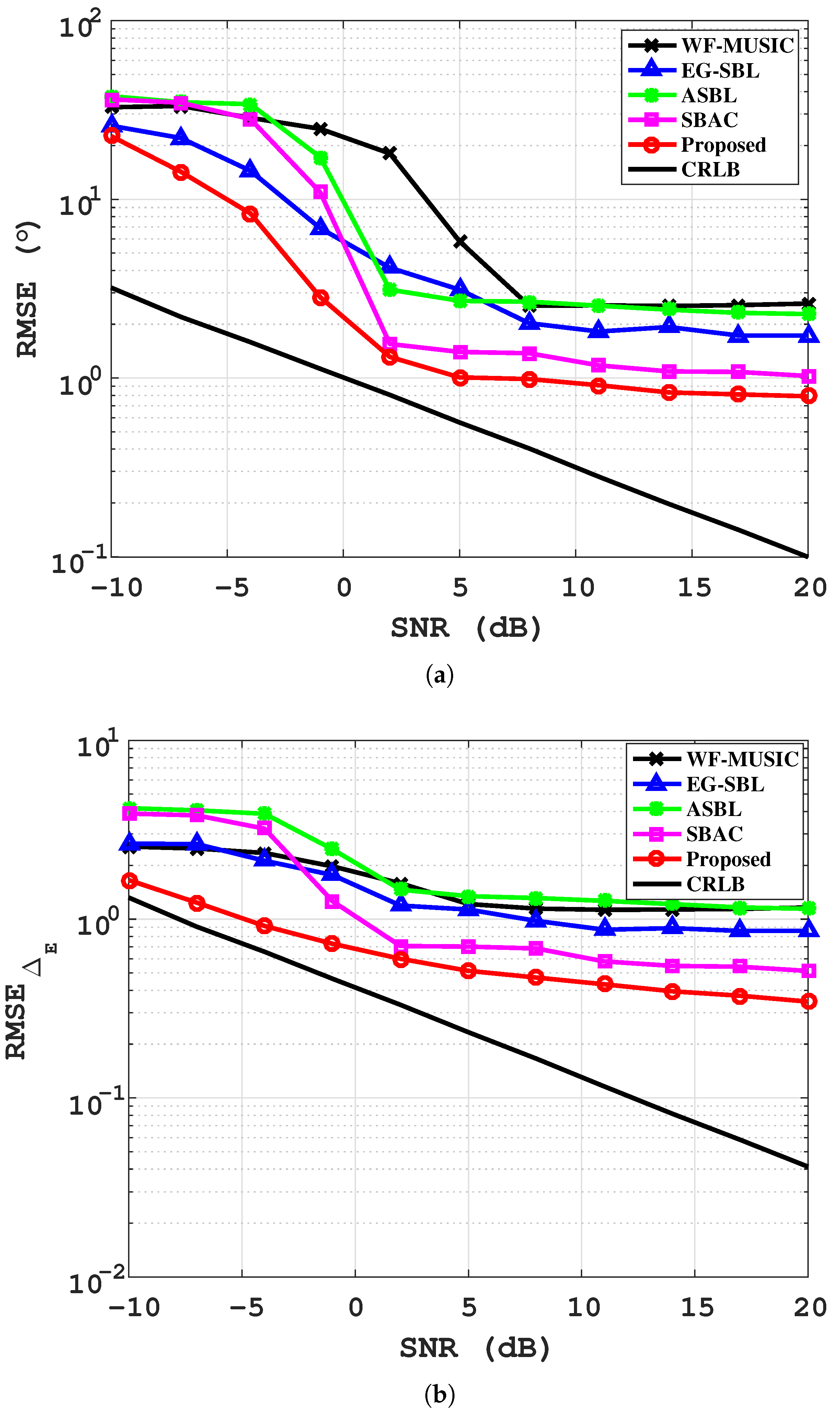
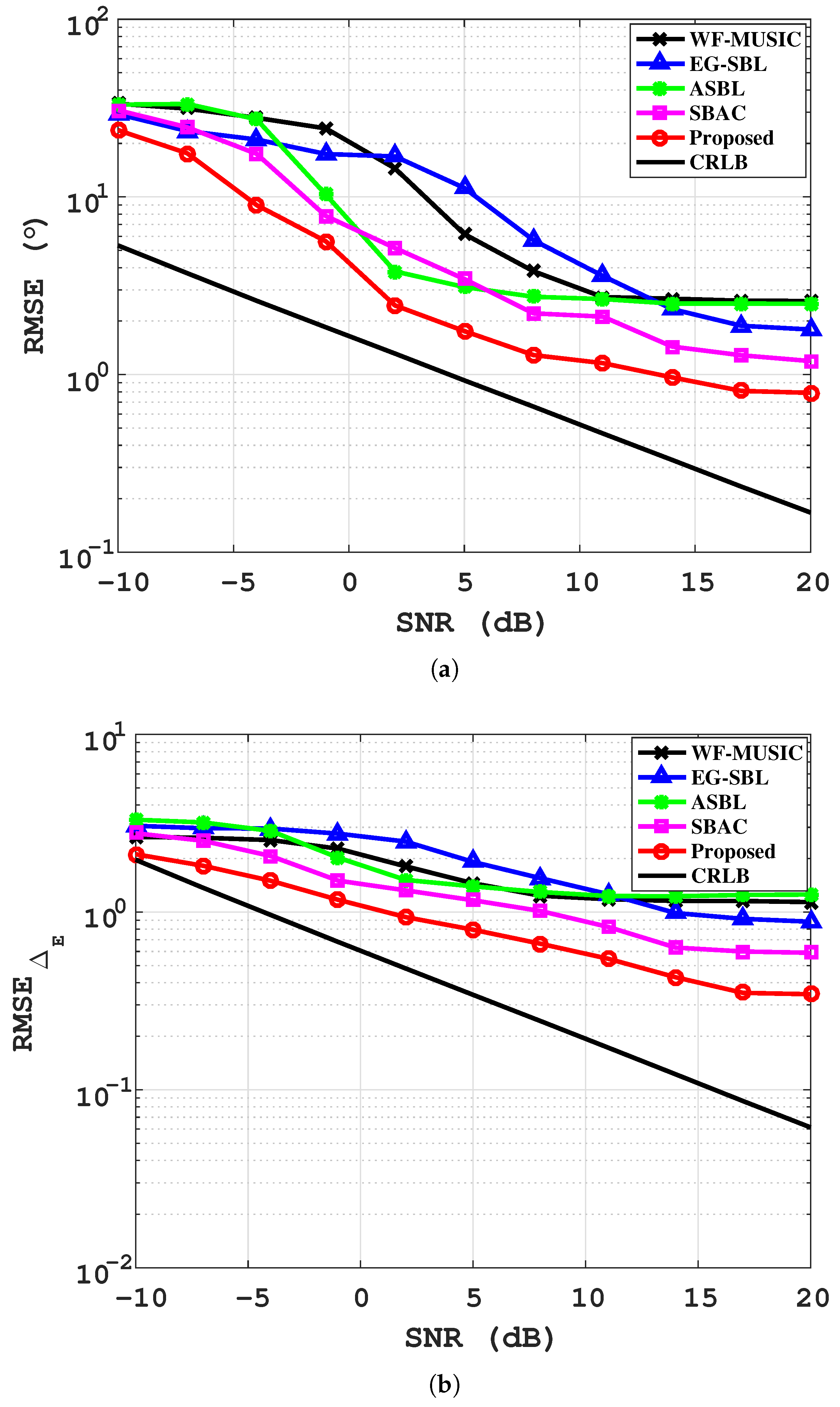
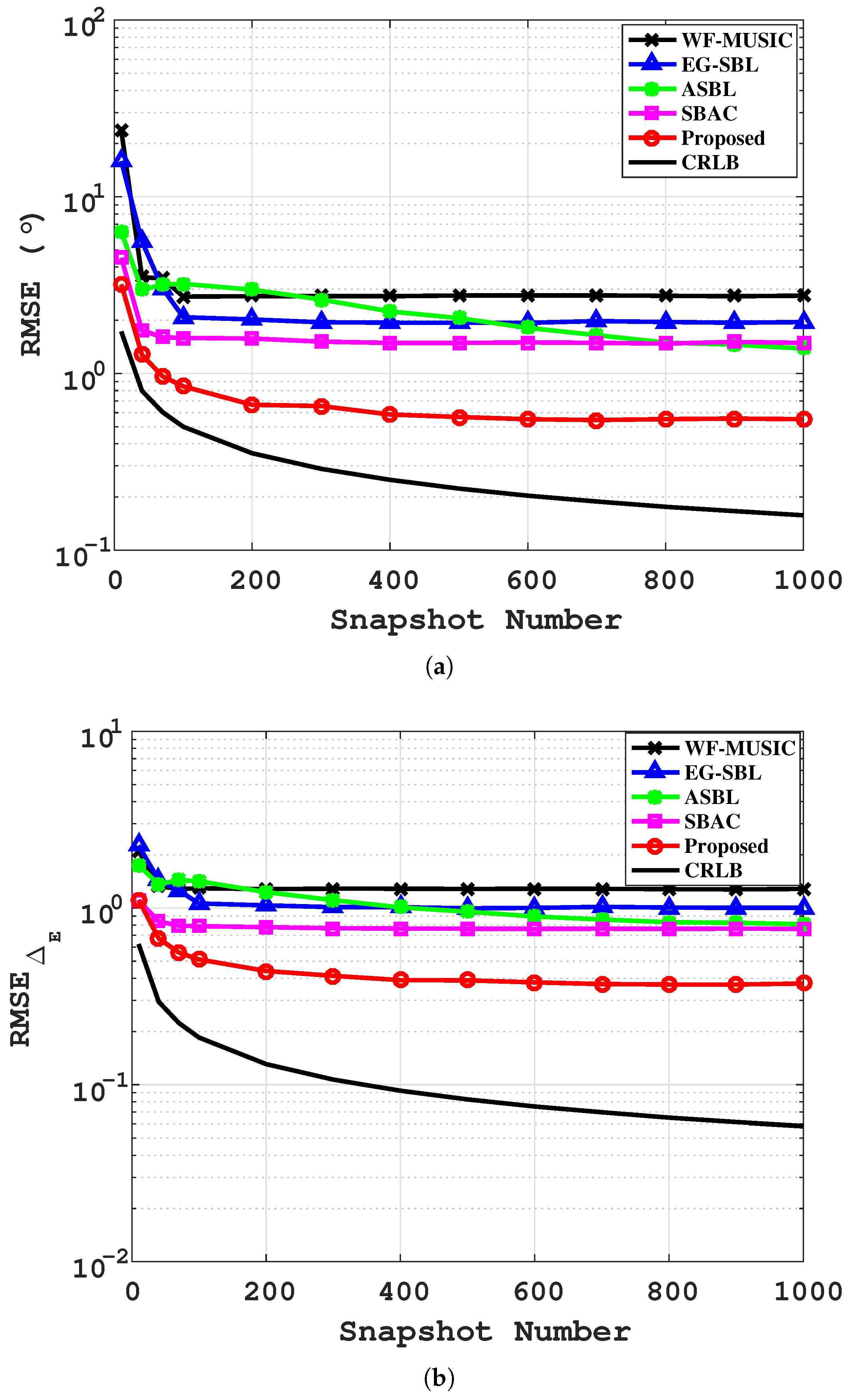
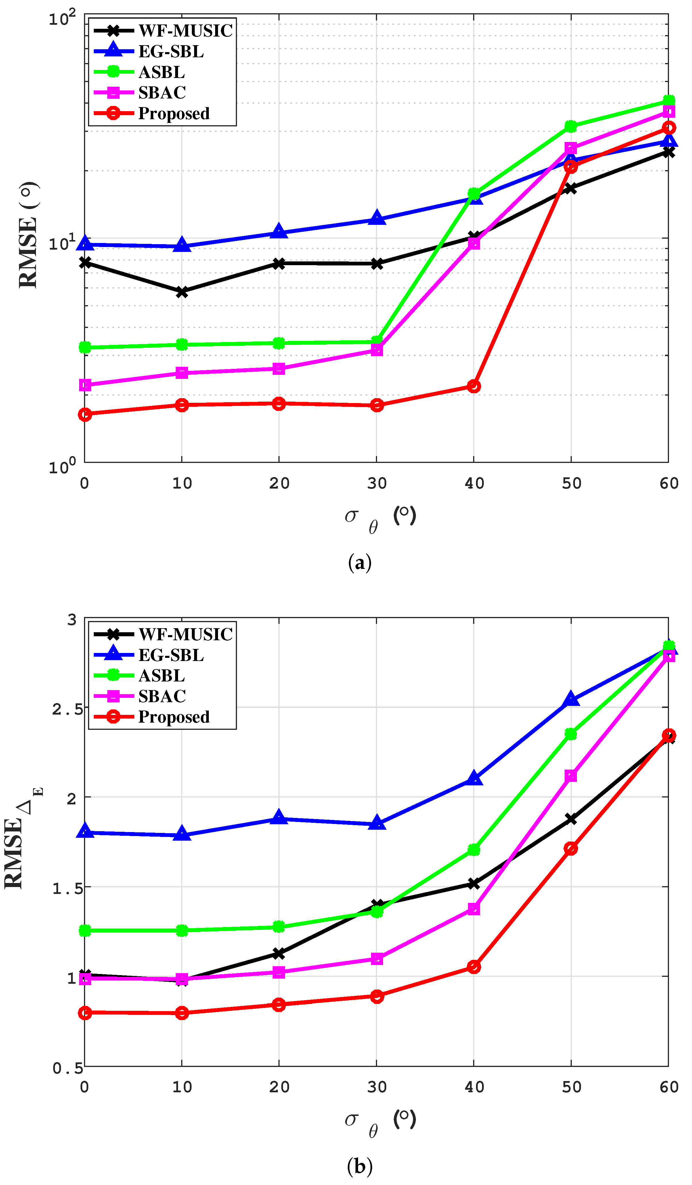
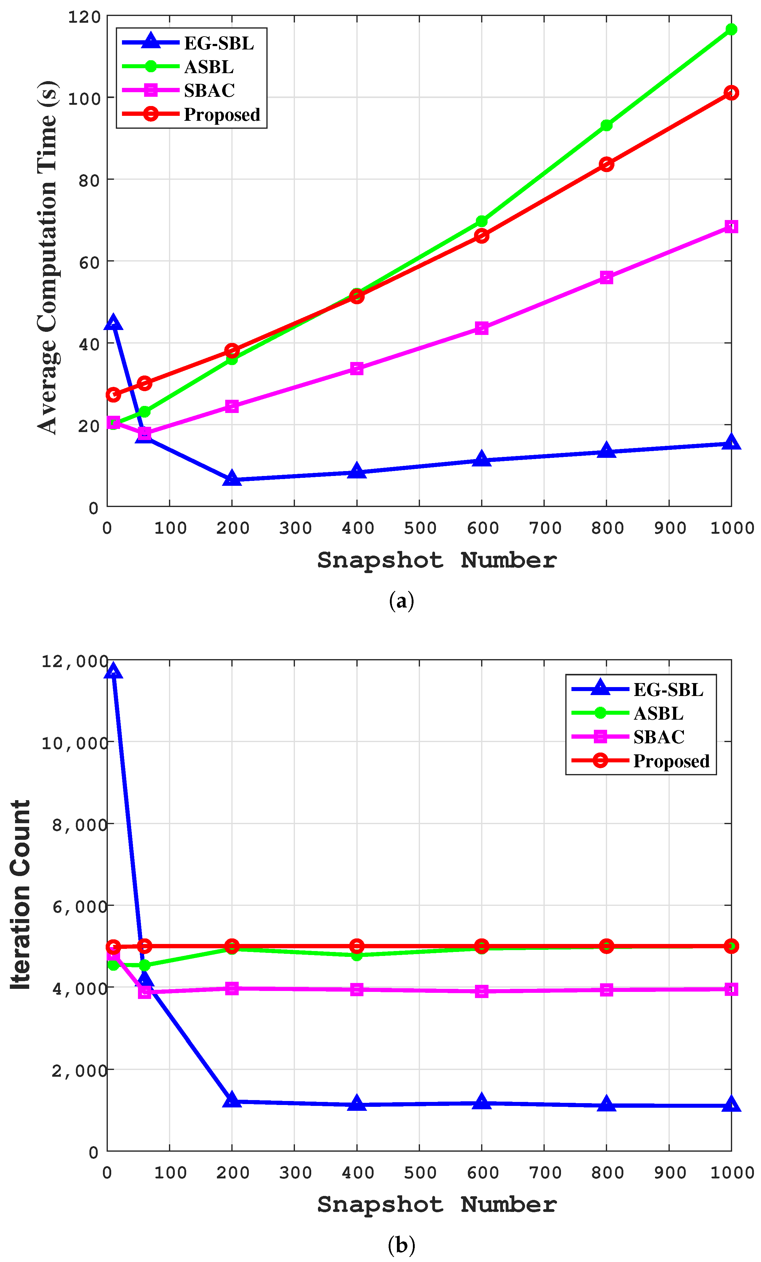
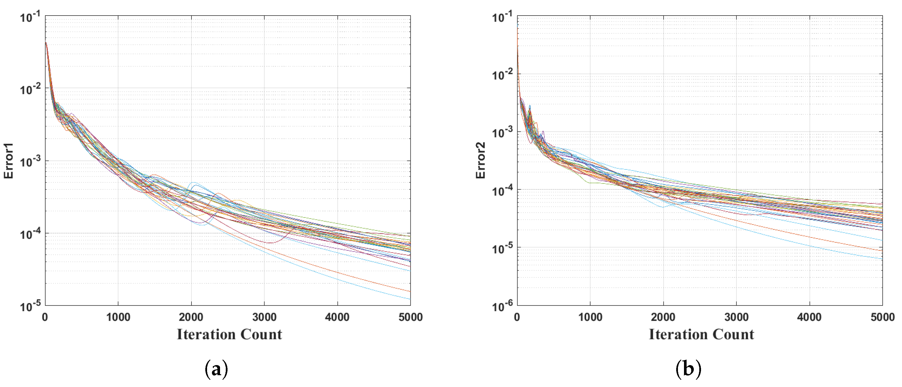
4.1. Simulation Results

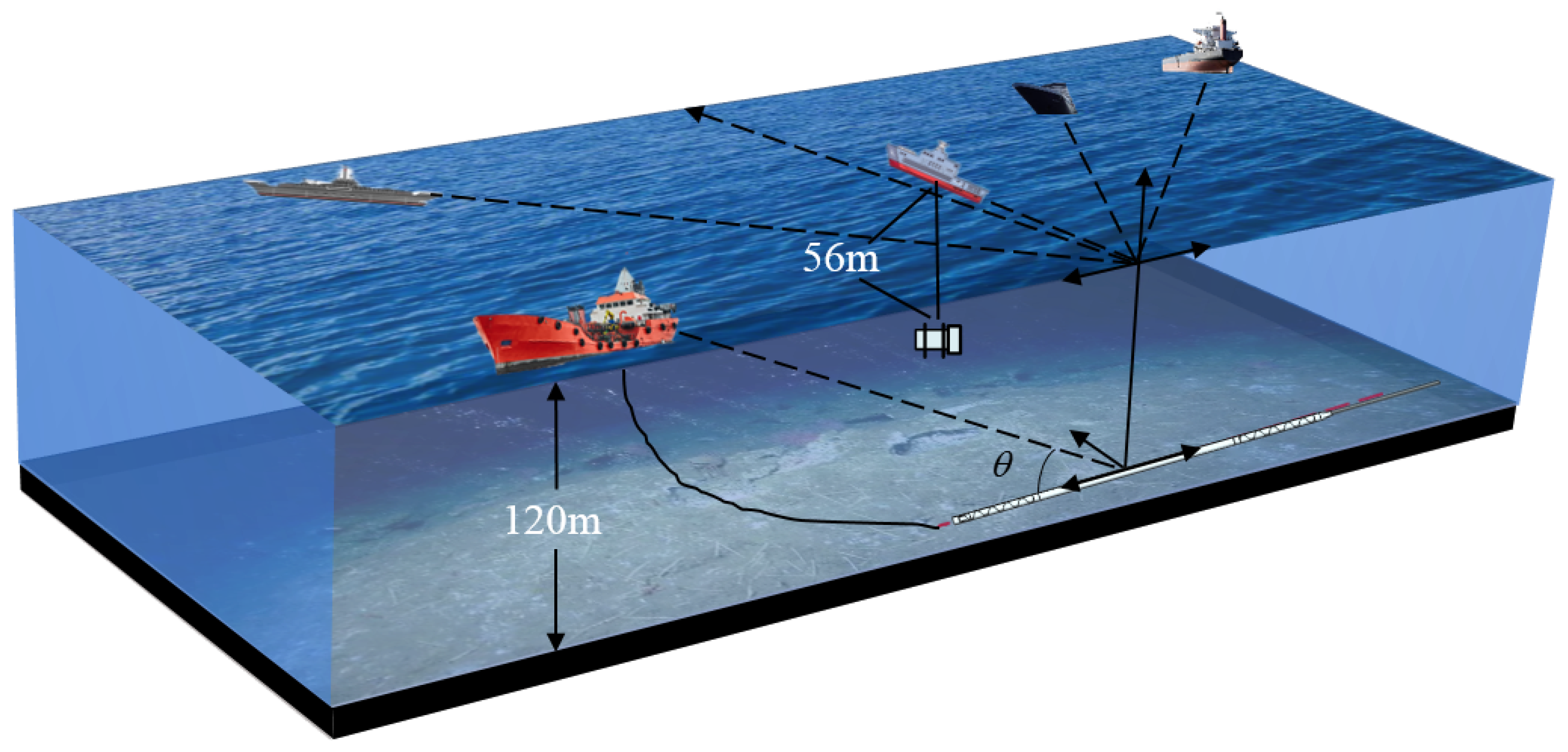
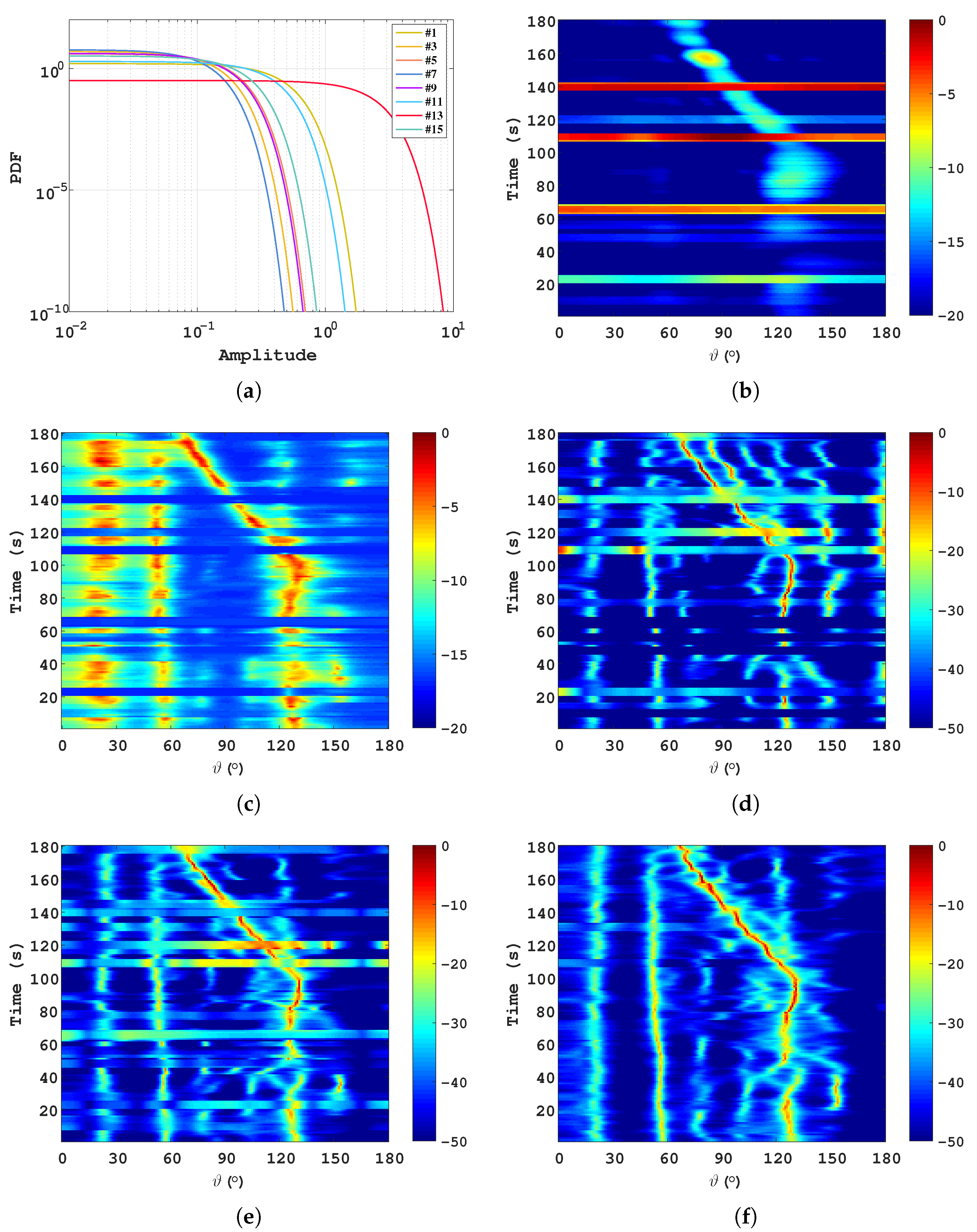
In this paper, the model errors considered include the gain error, phase error, and non-uniform ambient noise. It is assumed that two far-field signals are incident on the 10-element ULA from the ${110}^{\circ }$ and ${120}^{\circ }$ directions. The array gain and phase deviations settings in this subsection are referenced from [18]; the detailed settings are as follows: the gain errors are denoted by ${\Delta }_{\mathit{B}}=diag{\left\{0,0.15,0.3,0.2,0.25,-0.2,-0.2,-0.3,0.3,-0.15\right\}}^T$ and the phase errors are ${\Delta }_{\theta }={\left[0^{\circ },-{20}^{\circ },-{30}^{\circ },-{40}^{\circ },-{15}^{\circ },{35}^{\circ },{25}^{\circ },{20}^{\circ },{40}^{\circ },{15}^{\circ }\right]}^T$. The gain-phase error matrix ${\Delta }_{\mathit{E}}$ can be obtained from ${\Delta }_{\mathit{E}}={\Delta }_{\mathit{B}}{\Delta }_{\theta }$. The non-uniformity of the ambient noise is characterized by a Gaussian distribution, with different variances ${\sigma }_n^2\in {\left\{6,2,0.5,2.5,3,1,5.5,10,4,8\right\}}^T$.

For the non-uniform noise [23], the SNR is denoted as

$$\mathrm{SNR}=10lo{g}_{10}\left\{\sum _{n=1}^N{\displaystyle \frac{{\sigma }_s^2}{N{\sigma }_n^2}}\right\},$$

(48)

where ${\sigma }_s^2$ is the signal power. When the values of ${\sigma }_n^2$ are equal, the ambient noise is converted into uniform Gaussian noise.

The parameters involved in this subsection are defined as follows: the grid interval is $r=1^{\circ }$, the convergence threshold is $\epsilon ={10}^{-4}$, the maximum iterations is $maxiter=5000$, and the corresponding initial distribution parameters are indicated as ${10}^{-4}$. For the WF-MUSIC and EG-SBL methods, the criterion for distinguishing the signal subspace and the noise subspace is whether the eigenvalue percentage (summed up in descending order) exceeds $90\%$ of the sum. This criterion is employed to reduce the requirement for a priori information.

First, the spatial spectra of the proposed method and benchmark algorithms under different scenarios are illustrated in Figure 2, where two red pentagrams mark the predetermined target bearings. As shown in Figure 2a, all algorithms achieve accurate direction-of-arrival (DOA) estimations under ideal array geometry and uniform Gaussian noise conditions. In contrast, Figure 2b demonstrates the results in the presence of model errors, where all compared methods exhibit varying degrees of systematic estimation bias. The SBL algorithm fails to compensate for model errors, leading to significant performance degradation. Both WF-MUSIC and EG-SBL, rooted in eigenstructure-based frameworks, struggle to extract target features effectively in non-uniform noise environments. Additionally, ASBL and SBAC show high sensitivity to noise variance estimates, further degrading their robustness. Remarkably, the proposed method maintains estimation errors within 2° for both targets, demonstrating superior multi-target estimation capability under adverse conditions.

For the purpose of comparing the robustness and the joint estimation accuracy of these methods, the RMSEs are used to statistically analyse the bearing and gain-phase estimation results through 200 Monte Carlo experiments

$$\left\{\begin{array}{c}RMS{E}_{\Delta \vartheta }=\sqrt{{\displaystyle \frac{1}{ZT}}{\displaystyle \sum _{z=0}^{Z-1}}{\displaystyle \sum _{t=1}^T}{\left|{\vartheta }_z-{\tilde{\vartheta }}_{z,t}\right|}^2}\hfill \\ RMS{E}_{{\Delta }_{\mathit{E}}}=\sqrt{{\displaystyle \frac{1}{T}}{\displaystyle \sum _{t=1}^T}{∥{\Delta }_{\mathit{E}}-{\tilde{\Delta }}_{{\mathit{E}}_t}∥}_2^2}\hfill \end{array}\right..$$

(49)

where T and Z represent the number of Monte Carlo trails and incident signals, respectively. ${\vartheta }_z$ is the real direction for the zth signal, ${\Delta }_{\mathit{E}}$ expresses the pre-set gain-phase error matrix, and the superscript ∼ indicates the estimation of the corresponding parameter in each Monte Carlo experiment. In the simulation of statistical performance, the directions of these two targets are set as $\mathit{\vartheta }=\left\{{110}^{\circ }+\Delta ,{120}^{\circ }+\Delta \right\}$, where $\Delta$ represents the random bearings and is uniformly distributed with $\Delta \sim U\left(-0.5^{\circ },0.5^{\circ }\right)$ to eliminate a priori orientation that may be contained in the grid set $\overline{\mathit{\vartheta }}$.

Figure 3 presents the RMSE of DOA estimation and gain-phase calibration for WF-MUSIC, ASBL, EG-SBL, SBAC, and the proposed method under Gaussian noise conditions. The number of snapshots I is fixed at 30, with the SNR of both targets ranging from −10 dB to 20 dB. As shown in Figure 3b, the gain-phase estimation errors of all calibration algorithms decrease monotonically as SNR increases. However, WF-MUSIC, EG-SBL, and ASBL exhibit limited capability in mitigating large gain-phase biases, as evidenced by their persistent DOA estimation deviations of approximately $2^{\circ }$ in Figure 3a. This limitation stems from the eigenstructure-based calibration kernels of WF-MUSIC and EG-SBL, which fail to robustly separate signal and noise subspaces at low SNR regimes ($[-10,0]$ dB). Consequently, substantial gain-phase estimation errors propagate into their DOA results, degrading overall performance. In contrast, SBAC and the proposed method leverage the spatial sparsity of signals to jointly optimize amplitude-phase calibration and DOA estimation. The proposed method further outperforms SBAC by decoupling the magnitude and phase responses, enabling adaptive weighting of DOA precision constraints during optimization.

The SNR is fixed at 5 dB, and the number of receiving snapshots is increased from 10 to 1000. The RMSE comparison curves under different snapshot numbers are presented in Figure 4a,b. It can be observed that the WF-MUSIC and EG-SBL methods have a higher demand for the number of snapshots, leading to poor performance at small snapshots ($I\le 2N$). All algorithms perform smoothly as the number of snapshots increases. The SBAC and the proposed method can achieve stable and high-precision DOA estimation and gain-phase calibration with fewer snapshot numbers. This advantage is of great significance for increasing the realizability of engineering applications.

Then, the RMSEs in non-uniform noise for DOA estimation and gain-phase calibration are simulated in Figure 5 and Figure 6. The estimation curves of all compared methods are elevated relative to Figure 3 and Figure 4. The method proposed in this paper can still effectively estimate the gain-phase deviation in the non-uniform noise and obtain a higher accuracy of DOA estimation. The corresponding estimation results are quite similar to the results in the Gaussian noise, indicating that the proposed method can alleviate the performance degradation caused by the non-uniform noise.

It is worth noting that the performance degradation under low SNR conditions is a common challenge for all DOA estimation methods, particularly with limited array elements. For sparse Bayesian learning (SBL)-based approaches, which rely on the strict sparsity assumption (i.e., signals exist only at sparse angular directions), low SNR exacerbates the risk of noise being misidentified as weak signals. This violates the sparsity prior, leading to false peaks in DOA estimates. Additionally, the performance of all methods tends to stabilize without significant improvement when the SNR and snapshot numbers increase. The reason is that the target directions in each Monte Carlo simulation are deviated from the grid points, leading to inherent errors. During the joint iterative process, these inherent errors reduce the convergence accuracy of gain-phase calibration and hinder it from achieving better estimation results. Fortunately, the off-grid algorithm, which is discussed in [40,41], can help reduce the inherent error caused by grid partitioning. In our future exploration, we will also conduct further research on off-grid algorithms.

The aforementioned simulations are all implemented under a set of fixed amplitude and phase deviation. In order to further explore the tolerance range of the proposed method to amplitude and phase deviation, the effectiveness of each method under different amplitude and phase deviation is verified through the following simulations.

Considering that the array phase deviation is the primary factor affecting the performance of DOA estimation, the degree of phase deviation is adjusted. The phase deviation [36] of the n-th array element in each Monte Carlo experiment is

$${\theta }_n=\sqrt{12}{\sigma }_{\theta }{\varphi }_n,$$

(50)

where ${\varphi }_n$ denotes the random perturbation coefficient of the phase, which obeys a uniform distribution of ${\varphi }_n\sim U\left(-0.5,0.5\right)$. ${\sigma }_{\theta }$ denotes the standard deviation of the phase deviation fluctuation, and the larger ${\sigma }_{\theta }$ is, the greater is the inconsistency of the phase of each array element.

With a fixed SNR of 5 dB and a fast beat number of 30, ${\sigma }_{\theta }$ was changed from $0^{\circ }$ to ${50}^{\circ }$ and the other simulation conditions remained unchanged. The RMSE results of each method under different phase deviations are depicted in Figure 7. It is evident that the estimation performance of all the amplitude-phase calibration methods deteriorates to varying degrees as the phase deviation increases.

From Figure 7, we can observe that both the WF-MUSIC and EG-SBL methods are calibrated based on the feature structure, which requires a high number of snapshots and performs poorly in this condition. The ASBL and SBAC methods can calibrate the amplitude-phase deviation and obtain bearing estimation results more stably when the phase perturbation standard deviation is less than ${30}^{\circ }$. However, when the phase perturbation standard deviation is more than ${30}^{\circ }$, the performance of the two methods degrades seriously, and the deviation of the RMSE of the target bearing is more than ${10}^{\circ }$, which implies that the methods are invalid. Compared with other methods, the proposed method has better DOA estimation accuracy and amplitude-phase deviation estimation accuracy, and the standard deviation of phase disturbance tolerance is ${40}^{\circ }$. When the standard deviation of the phase disturbance is less than ${40}^{\circ }$, the estimated deviation of the target orientation is less than $3^{\circ }$, which indicates that the proposed method has better tolerance of phase deviation than other comparison methods.

Next, we analyze the computational complexity and runtime of all the sparse direction-finding methods. The high computational complexity of these methods primarily stems from matrix inversion operations. Using Big O notation for analysis, the classic SBL method exhibits a computational complexity of $O\left(N^3\right)$ per iteration, where N denotes the number of grid points. The EG-SBL method, which combines eigen-subspace techniques with SBL, iteratively estimates amplitude-phase deviations using SBL for DOA correction and then updates these deviations. Consequently, its complexity escalates to $O\left(K{N}^3\right)$, where K represents the iteration count of the eigen-subspace process. In contrast, ASBL, SBAC, and the proposed method focus primarily on amplitude-phase deviation estimation without introducing additional complexity beyond $O\left(N^3\right)$, resulting in computational costs comparable to SBL.

While this comparison neglects minor complexity accumulations, we further evaluate practical runtime performance by measuring the execution times and iteration counts across varying snapshot counts under the simulation setup of Figure 2.All experiments were conducted on an Intel^® Core™ i5-7500 CPU (Lenovo, Beijing, China) @3.40 GHz with 8 GB RAM, with the results summarized in Figure 8.

Figure 8a reveals that the average runtime of all methods grows linearly with the snapshot counts. This trend arises because matrix multiplication operations in sparse Bayesian frameworks depend on the snapshot numbers, thereby increasing overall complexity. However, significant runtime disparities emerge among methods, attributable to their divergent iteration requirements. As evidenced by Figure 8b, EG-SBL requires the fewest iterations, resulting in the shortest average runtime. In contrast, the SBAC method converges approximately 1000 iterations faster than both ASBL and the proposed method when reaching the convergence threshold, leading to a notable runtime advantage. This implies that the proposed method struggles to achieve real-time processing in practical engineering applications. A potential solution is to incorporate off-grid techniques to reduce the overall computational complexity, thereby enhancing feasibility for real-time implementation. Notably, EG-SBL exhibits excessive runtime and iterations at low snapshot counts (Figure 8b), as insufficient snapshots degrade eigen-subspace separation, impairing amplitude-phase estimation. This issue alleviates as the snapshots increase.

To further validate the convergence behavior of the proposed method, we define the following error metrics to assess its convergence characteristics

$$Error1={\displaystyle \frac{{∥{\mathit{\eta }}^{\mathrm{new}}-{\mathit{\eta }}^{old}∥}_2}{{∥{\mathit{\eta }}^{old}∥}_2}},$$

(51)

$$Error2={\displaystyle \frac{{∥diag\left({\Delta \mathit{E}}^{\mathrm{new}}\right)-diag\left({\Delta \mathit{E}}^{old}\right)∥}_2}{{∥diag\left({\Delta \mathit{E}}^{old}\right)∥}_2}},$$

(52)

$$Error3={∥diag\left({\Delta \mathit{E}}^{\mathrm{new}}\right)-diag\left(\Delta {\mathit{E}}_r\right)∥}_2,$$

(53)

Here, $Error1$ quantifies the fluctuation between the latest iteration ${\mathit{\eta }}^{\mathrm{new}}$ and the previous iteration ${\mathit{\eta }}^{\mathrm{old}}$ of the signal variance precision vector $\mathit{\eta }$, while $Error2$ measures the fluctuation between the latest iteration ${\Delta \mathit{E}}^{\mathrm{new}}$ and the previous iteration ${\Delta \mathit{E}}^{\mathrm{old}}$ of the amplitude-phase deviation matrix $\Delta \mathit{E}$. These two metrics serve as convergence criteria to evaluate whether the proposed method has converged. Additionally, $Error3$ represents the discrepancy between the estimated results at each iteration and the ground truth $\Delta {\mathit{E}}_r$. By analyzing $Error3$ alongside the DOA estimates from each iteration, we can assess the convergence validity of the algorithm.

Thirty independent Monte Carlo trials were conducted to ensure intuitive and reliable results, as depicted in Figure 9. Each curve represents a single Monte Carlo iteration process, with the solid red line in Figure 9d indicating the ground truth bearings. The results demonstrate that the initial parameter settings, which significantly deviate from the true values, induce pronounced fluctuations across all metrics during early iterations. These fluctuations gradually stabilize as the algorithm progresses, exhibiting a clear convergence trend where the estimated bearings approach the ground truth. Furthermore, the alternating updates between the amplitude-phase parameters and the signal variance introduce intermittent oscillations due to their mutual coupling effects. However, such oscillations diminish rapidly without compromising the convergence validity, as evidenced by the monotonic convergence of metric $Error3$. Overall, all parameter estimates converge stably despite transient perturbations.

4.2. Experiment

In this section, all comparison methods are utilized to process the sea trial data to validate the calibration ability and robustness for model errors.

The first set of experimental data were recorded via a 20-element submarine optical-fiber array, with each array being uniformly distributed at 8 m intervals on the shallow seabed. The distance between the sound source vessel and the receiving vessel is approximately 15 km. The transmitting transducer was hoisted and sonar signals of varying intensities were emitted intermittently. The test diagram is shown in Figure 10.

In the data processing, the observation interval $(0^{\circ },{180}^{\circ })$ is uniformly divided into 181 grid points. The convergence threshold is set to $\epsilon ={10}^{-3}$, and the maximum number of iterations is set at 1000. Each processing time takes approximately 6 s with 23 snapshots, resulting in a total processing time of 990 s. The processing results of all the algorithms are given in Figure 11.

Figure 11a presents the statistical characteristics of the 7-channel received data for the array, which are fitted with a Gaussian distribution. The results indicate that the noise in each channel follows an identical Gaussian distribution with approximately equal variance across channels. To benchmark the calibration performance, we employ the conventional beamforming (CBF) algorithm [42]—a widely adopted engineering reference method. Figure 11b shows the results of the CBF method, the strong target near ${30}^{\circ }$ is the array-connected vessel, while the target near ${92}^{\circ }$ is an acoustic source vessel that is transmitting signals intermittently during the processing time. The black dotted line in the figure indicates the GPS recording track. The CBF method observes fewer targets and shows distortions at certain processing moments, such as 620 s, 760 s, 850 s, and 880 s. Figure 11c,d gives the BTMs of all the compared self-calibration algorithms. It can be observed that all methods demonstrate good estimation performance under Gaussian noise. In particular, the ASBL, SBAC and the proposed method are more capable of discriminating multiple targets. However, ASBL is less robust and shows more transverse spikes in the BTM, which affects the clarity of the trajectory. On the other hand, the SBAC and proposed method obtain better estimation results than the other methods. Nevertheless, as shown in Figure 11e, SBAC also experiences varying degrees of performance loss near the 620 s, 760 s, and 880 s moments. This negatively impacts the quality of the trajectory observation. The proposed method effectively overcomes such distortion and provides clearer trajectories.

In order to verify the accuracy of each method for calibrating the model errors, the estimation results of each method are compared with the GPS recording track, and the RMSE results are calculated to assess the calibration performance through the DOA estimation accuracy. The results in

Table 1. RMSE results of various methods for acoustic vessel track observation.

Algorithm	CBF	WF-MUSIC	ASBL	SBAC	Proposed
RMSE (°)	1.533	1.159	0.949	0.509	0.483

demonstrate that the proposed method has the better DOA estimation accuracy and that the estimated bearing is closest to the GPS track. These findings indicate that the method has superior calibration performance.

The second set of experimental data was recorded via a 16-element submarine optical-fiber array, distributed uniformly at a distance of 8m on the shallow seabed. The water depth of the experimental area was 20 m. Prior to deployment, the channel was debugged to ensure good gain-phase consistency, i.e., ${\Delta }_{\mathit{E}}=\mathbf{0}$. The main shipping lanes surrounded the experimental sea area, and the other vessels traveling on the lanes were used as targets for passive detection. In data processing, the observation interval $[0^{\circ },{180}^{\circ }]$ is uniformly divided into 181 grid points. The convergence threshold is $\epsilon ={10}^{-3}$, and the maximum number of iterations is 1000. Each processing time is 5 s with 19 snapshots, and the total processing time is 180 s. The processing results of all the algorithms are given in Figure 12.

Figure 12a presents the statistical characteristics of the 8-channel received data for the array, which are fitted with a Gaussian distribution. It can be seen that the noise received by each channel contains apparent non-uniformity, indicating the necessity for researching the gain-phase calibration under non-uniform noise. Figure 12b–f provides the BTMs of all the compared algorithms. In Figure 12b, the CBF method only observes a clear target trajectory; it produces a lot of cluttered spikes under the influence of non-uniform noise, which seriously degrades the estimation performance. Figure 12c demonstrates the results of the WF-MUSIC algorithm. As a high-precision algorithm, it can distinguish the target trajectories near ${30}^{\circ }$ and ${60}^{\circ }$. However, the motion trajectories appear blurred due to the eigenstructure being corrupted by non-uniform noise. The ASBL, SBAC and the proposed method are based on the sparse Bayesian framework. As depicted in Figure 12d–f, they provide higher accuracy and more evident target trajectories. However, both the ASBL and SBAC results produce varying degrees of cluttered spikes due to their inability to combat non-uniform noise. These spikes affect the coherence of the motion trajectory and may mask the trajectory of weak targets. Notably, the DOA estimation of Figure 12d produces a shift relative to Figure 12e,f during the observation epochs of 20–70 s. It indicates that the ASBL does not perform gain-phase calibration well at fewer snapshots, which is also consistent with the simulation analysis in Figure 6. It is predictable that more snapshots can effectively improve the performance of ASBL. However, the inclusion of a substantial cumulative duration may have an adverse effect on the estimation performance of moving targets. As shown in Figure 12f, the target trajectory obtained by the proposed method is more explicit and more coherent, and there are almost no clutter spikes, which indicates the superiority of the proposed method in combating non-uniform noise.

In order to facilitate a more explicit comparison of the performance of these algorithms, the spatial spectrum results at t = 24 s and t = 25 s are given in Figure 13. It can be observed that CBF and WF-MUSIC have high noise levels and broader peaks relative to the other algorithms, which is not conducive to discriminating between weak and nearby targets. ASBL and SBAC are unable to estimate the target efficiently at t = 24 s. However, the proposed algorithm is still capable of estimating multiple target orientations, indicating that it has greater robustness than other approaches. Furthermore, the gain-phase calibration deviation of each method can be calculated by (49), and the corresponding results are displayed in

Table 2. The gain-phase calibration deviations of all comparison algorithms.

Algorithm	WF-MUSIC	ASBL	SBAC	Proposed
Error	4.163	1.585	0.292	0.194

. It can be observed that the gain-phase calibration result of the proposed method is superior to that of the other methods.

5. Discussion

While the proposed method demonstrates advantages over conventional subspace-based approaches, it inherently exhibits higher computational complexity. Additionally, the grid-based framework cannot inherently correct the bias in DOA estimation caused by grid discretization, resulting in sensitivity to grid resolution. Finer grids can improve accuracy but significantly escalate computational demands. A promising solution lies in integrating off-grid techniques to extend the proposed method into an off-grid signal processing framework. This adaptation not only enhances the estimation accuracy for targets located off the predefined grid but also reduces computational complexity through sparse reconstruction. Further exploration of this direction will constitute a key focus of our future research efforts.

6. Conclusions

A self-calibration method based on VBI under model errors has been proposed and verified. This method has been shown to yield superior calibration results for gain and phase errors and to provide an excellent DOA estimation performance in the presence of non-uniform noise. The proposed sparse recovery model constructs the gain, phase and noise power of each element as independent parameters, and VBI is used to derive iterative solutions for the above parameters. The comparisons and analyses of the proposed method and the existing approaches are given and discussed. Simulations and experimental results verify that the proposed method can yield superior performance in DOA estimations and gain-phase calibrations.

References

1. Wang, S.; Wang, H.; Bian, Z.; Chen, S.; Song, P.; Su, B.; Gao, W. A Robust Direction-of-Arrival (DOA) Estimator for Weak Targets Based on a Dimension-Reduced Matrix Filter with Deep Nulling and Multiple-Measurement-Vector Orthogonal Matching Pursuit. Remote Sens. 2025, 17, 477. [Google Scholar] [CrossRef]
2. Yazdi, N.; Todros, K. Measure-Transformed MVDR Beamforming. IEEE Signal Process. Lett. 2020, 27, 1959–1963. [Google Scholar] [CrossRef]
3. Huang, L.; So, H.C. Source Enumeration via MDL Criterion Based on Linear Shrinkage Estimation of Noise Subspace Covariance Matrix. IEEE Trans. Signal Process. 2013, 61, 4806–4821. [Google Scholar] [CrossRef]
4. Blasone, G.P.; Colone, F.; Lombardo, P.; Wojaczek, P.; Cristallini, D. Passive Radar STAP Detection and DoA Estimation Under Antenna Calibration Errors. IEEE Trans. Aerosp. Electron. Syst. 2021, 57, 2725–2742. [Google Scholar] [CrossRef]
5. Li, C.; Liang, G.; Qiu, L.; Shen, T.; Zhao, L. An efficient sparse method for direction-of-arrival estimation in the presence of strong interference. J. Acoust. Soc. Am. 2023, 153, 1257–1271. [Google Scholar]
6. Wang, X.; Sun, H.; Zhang, L.; Dong, C.-P.; Guo, L.-X. Unambiguous broadband direction of arrival estimation based on improved extended frequency-difference method. J. Acoust. Soc. Am. 2022, 152, 3281–3293. [Google Scholar]
7. Liao, B.; Wen, J.; Huang, L.; Guo, C.; Chan, S.C. Direction Finding With Partly Calibrated Uniform Linear Arrays in Nonuniform Noise. IEEE Sens. J. 2016, 16, 4882–4890. [Google Scholar] [CrossRef]
8. Barry, N.; Hazelton, B.; Sullivan, I.; Morales, M.; Pober, J. Calibration requirements for detecting the 21 cm epoch of reionization power spectrum and implications for the SKA. Mon. Not. R. Astron. Soc. 2016, 461, 3135–3144. [Google Scholar]
9. Long, R.; Ouyang, J.; Yang, F.; Han, W.; Zhou, L. Multi-Element Phased Array Calibration Method by Solving Linear Equations. IEEE Trans. Antennas Propag. 2017, 65, 2931–2939. [Google Scholar] [CrossRef]
10. Weiss, A.J.; Friedlander, B. Eigenstructure methods for direction finding with sensor gain and phase uncertainties. Circuits Syst. Signal Process. 1990, 9, 271–300. [Google Scholar]
11. Dai, Z.; Su, W.; Gu, H.; Li, W. Sensor Gain-Phase Errors Estimation Using Disjoint Sources in Unknown Directions. IEEE Sens. J. 2016, 16, 3724–3730. [Google Scholar] [CrossRef]
12. Liu, A.; Liao, G.; Zeng, C.; Yang, Z.; Xu, Q. An Eigenstructure Method for Estimating DOA and Sensor Gain-Phase Errors. IEEE Trans. Signal Process. 2011, 59, 5944–5956. [Google Scholar] [CrossRef]
13. Mohsen, N.; Hawbani, A.; Wang, X.; Bairrington, B.; Zhao, L.; Alsamhi, S. New Array Designs for DoA Estimation of Non-Circular Signals with Reduced Mutual Coupling. IEEE Trans. Veh. Technol. 2023, 72, 8313–8328. [Google Scholar] [CrossRef]
14. Liu, H.; Zhao, L.; Li, Y.; Jing, X.; Truong, T.K. A Sparse-Based Approach for DOA Estimation and Array Calibration in Uniform Linear Array. IEEE Sens. J. 2016, 16, 6018–6027. [Google Scholar] [CrossRef]
15. Badiu, M.A.; Hansen, T.L.; Fleury, B.H. Variational Bayesian Inference of Line Spectra. IEEE Trans. Signal Process. 2017, 65, 2247–2261. [Google Scholar] [CrossRef]
16. Sun, D.; Fu, X.; Teng, T. A Deep Learning Localization Method for Acoustic Source via Improved Input Features and Network Structure. Remote Sens. 2024, 16, 1391. [Google Scholar] [CrossRef]
17. Zhao, L.; Bi, G.; Wang, L.; Zhang, H. An Improved Auto-Calibration Algorithm Based on Sparse Bayesian Learning Framework. IEEE Signal Process. Lett. 2013, 20, 889–892. [Google Scholar] [CrossRef]
18. Li, Z.; Huang, Z. Sparse Bayesian learning based DOA estimation and array gain-phase error self-calibration. Prog. Electromagn. Res. M 2022, 108, 65–77. [Google Scholar] [CrossRef]
19. Liu, Z.M.; Zhou, Y.Y. A Unified Framework and Sparse Bayesian Perspective for Direction-of-Arrival Estimation in the Presence of Array Imperfections. IEEE Trans. Signal Process. 2013, 61, 3786–3798. [Google Scholar] [CrossRef]
20. Lu, R.; Zhang, M.; Liu, X.; Chen, X.; Zhang, A. Direction-of-Arrival Estimation via Coarray with Model Errors. IEEE Access 2018, 6, 56514–56525. [Google Scholar] [CrossRef]
21. Chen, Z.; Ma, W.; Chen, P.; Cao, Z. A Robust Sparse Bayesian Learning-Based DOA Estimation Method with Phase Calibration. IEEE Access 2020, 8, 141511–141522. [Google Scholar] [CrossRef]
22. Zhou, X.; Fan, B.; Wang, H.; Cheng, Y.; Qin, Y. Sparse Bayesian Perspective for Radar Coincidence Imaging with Array Position Error. IEEE Sens. J. 2017, 17, 5209–5219. [Google Scholar] [CrossRef]
23. Yu, D.; Wang, X.; Fang, W.; Ma, Z.; Lan, B.; Song, C.; Xu, Z. DOA Estimation Based on Root Sparse Bayesian Learning Under Gain and Phase Error. J. Commun. Inf. Netw. 2022, 7, 202–213. [Google Scholar] [CrossRef]
24. Liao, B.; Chan, S.C.; Huang, L.; Guo, C. Iterative Methods for Subspace and DOA Estimation in Nonuniform Noise. IEEE Trans. Signal Process. 2016, 64, 3008–3020. [Google Scholar] [CrossRef]
25. Guo, K.; Zhang, L.; Li, Y.; Zhou, T.; Yin, J. Variational Bayesian Inference for DOA Estimation Under Impulsive Noise and Nonuniform Noise. IEEE Trans. Aerosp. Electron. Syst. 2023, 59, 5778–5790. [Google Scholar] [CrossRef]
26. Song, J.; Cao, L.; Zhao, Z.; Yang, K.; Wang, D.; Fu, C. Robust Gridless DOA Estimation Using Coprime Array Under Nonuniform Noise. IEEE Trans. Instrum. Meas. 2025, 74, 6502017. [Google Scholar] [CrossRef]
27. Liu, Z.M.; Zhang, C.; Philip, S.Y. Direction-of-arrival estimation based on deep neural networks with robustness to array imperfections. IEEE Trans. Antennas Propag. 2018, 66, 7315–7327. [Google Scholar] [CrossRef]
28. Abdullah, M.; Li, M.S.; He, J.; Wang, K.; Fumeaux, C.; Withayachumnankul, W. Direction of Arrival Estimation in Terahertz Communications using Convolutional Neural Networks. In Proceedings of the 2024 49th International Conference on Infrared, Millimeter, and Terahertz Waves (IRMMW-THz), Perth, Australia, 1–6 September 2024. [Google Scholar]
29. Wu, L.; Liu, Z.M.; Huang, Z.T. Deep convolution network for direction of arrival estimation with sparse prior. IEEE Signal Process. Lett. 2019, 26, 1688–1692. [Google Scholar] [CrossRef]
30. Islam, A.; Long, C.; Basharat, A.; Hoogs, A. DOA-GAN: Dual-order attentive generative adversarial network for image copy-move forgery detection and localization. In Proceedings of the 2020 IEEE/CVF Conference on Computer Vision and Pattern Recognition (CVPR), Seattle, WA, USA, 13–19 June 2020; pp. 4676–4685. [Google Scholar]
31. Mylonakis, C.M.; Velanas, P.; Lazaridis, P.I.; Sarigiannidis, P.; Goudos, S.K.; Zaharis, Z.D. Deep Learning Framework Using Spatial Attention Mechanisms for Adaptable Angle Estimation Across Diverse Array Configurations. Technologies 2025, 13, 46. [Google Scholar] [CrossRef]
32. Fu, X.; Sun, D.; Teng, T. A high-resolution method for direction of arrival estimation based on an improved self-attention module. J. Acoust. Soc. Am. 2024, 156, 2743–2758. [Google Scholar] [CrossRef]
33. Tzikas, D.G.; Likas, A.C.; Galatsanos, N.P. The variational approximation for Bayesian inference. IEEE Signal Process. Mag. 2008, 25, 131–146. [Google Scholar]
34. Kvalseth, T. Generalized divergence and Gibbs’ inequality. In Proceedings of the 1997 IEEE International Conference on Systems, Man, and Cybernetics. Computational Cybernetics and Simulation, Orlando, FL, USA, 12–15 October 1997; Volume 2, pp. 1797–1801. [Google Scholar] [CrossRef]
35. Chen, G.; Su, X.; He, L.; Guan, D.; Liu, Z. Coherent Signal DOA Estimation Method Based on Space–Time–Coding Metasurface. Remote Sens. 2025, 17, 218. [Google Scholar] [CrossRef]
36. Pesavento, M.; Gershman, A. Maximum-likelihood direction-of-arrival estimation in the presence of unknown nonuniform noise. IEEE Trans. Signal Process. 2001, 49, 1310–1324. [Google Scholar] [CrossRef]
37. Dai, E.; Su, L.; Ge, Y. Cramer-Rao lower bound for frequency estimation of sinusoidal signals. IEEE Trans. Instrum. Meas. 2024, 73, 6503507. [Google Scholar]
38. Tian, J.; Yang, M.; Ni, S.; Chao, T. The CRLB for target localization using Gaussian process regression with distance-dependent noise. Measurement 2024, 226, 114127. [Google Scholar] [CrossRef]
39. Sang, Y.; Ji, X.; Wei, D.; You, Y.; Zhang, W. Cramer-Rao Lower Bound for Geomagnetic Matching and Its Approximation Method. IEEE Trans. Aerosp. Electron. Syst. 2025. early access. [Google Scholar]
40. Guo, Q.; Xin, Z.; Zhou, T.; Xu, S. Off-Grid Space Alternating Sparse Bayesian Learning. IEEE Trans. Instrum. Meas. 2023, 72, 1002310. [Google Scholar] [CrossRef]
41. Zhu, J.; Zhang, Q.; Gerstoft, P.; Badiu, M.A.; Xu, Z. Grid-less variational Bayesian line spectral estimation with multiple measurement vectors. Signal Process. 2019, 161, 155–164. [Google Scholar]
42. González-Coma, J.P.; Nocelo López, R.; Núñez-Ortuño, J.M.; Troncoso-Pastoriza, F. Beacon-Based Phased Array Antenna Calibration for Passive Radar. Remote Sens. 2025, 17, 490. [Google Scholar] [CrossRef]
Figure 1. Algorithmic graphical model.
Remotesensing 17 01319 g001
Figure 2. The spatial spectrum of the proposed method and the compared methods in different circumstances, where SNR = 5 dB, N = 10 and I = 30 . (a) Array condition is perfect; (b) Array has gain and phase deviations and exists in non-uniform noise environments.
Remotesensing 17 01319 g002
Figure 3. The effects comparison of WF-MUSIC, ASBL, EG-SBL, SBAC and proposed method in Gaussian noise versus SNR, where N = 10 and I = 30 . (a) RMSE comparisons of the DOA estimation results; (b) RMSE comparisons of the gain-phase calibration results.
Remotesensing 17 01319 g003
Figure 4. The effects comparison of WF-MUSIC, ASBL, EG-SBL, SBAC and the proposed method in Gaussian noise versus snapshots, where N = 10 and SNR = 5 dB. (a) RMSE comparisons of the DOA estimation results; (b) RMSE comparisons of the gain-phase calibration results.
Remotesensing 17 01319 g004
Figure 5. The effects comparison of WF-MUSIC, ASBL, EG-SBL, SBAC and the proposed method in non-uniform noise versus SNR, where N = 10 and I = 30 . (a) RMSE comparisons of the DOA estimation results; (b) RMSE comparisons of the gain-phase calibration results.
Remotesensing 17 01319 g005
Figure 6. The effects comparison of WF-MUSIC, ASBL, EG-SBL, SBAC and the proposed method in non-uniform noise versus snapshots, where N = 10 and SNR = 5 dB. (a) RMSE comparisons of the DOA estimation results; (b) RMSE comparisons of the gain-phase calibration results.
Remotesensing 17 01319 g006
Figure 7. The effects comparison of WF-MUSIC, ASBL, EG-SBL, SBAC and the proposed method in different phase deviations. (a) RMSE comparisons of the DOA estimation results; (b) RMSE comparisons of the gain-phase calibration results.
Remotesensing 17 01319 g007
Figure 8. Quantitative analysis of computational complexity across methods under varying snapshot counts. (a) Average runtime comparison; (b) Iteration count comparison.
Remotesensing 17 01319 g008
Figure 9. Convergence analysis of iterative parameter estimation in the proposed method. (a) Self-convergence of parameter η ; (b) Self-convergence of parameter Δ E ; (c) Deviation of parameter Δ E from ground truth Δ E r ; (d) DOA estimation results.
Remotesensing 17 01319 g009aRemotesensing 17 01319 g009b
Figure 10. Diagram of test arrangement.
Remotesensing 17 01319 g010
Figure 11. The statistical characteristics of the received signal and the BTMs of the different algorithms, where N = 20 and I = 23 . (a) The statistical characteristics of received signal; (b) BTM of CBF algorithm; (c) BTM of WF-MUSIC algorithm; (d) BTM of ASBL algorithm; (e) BTM of SBAC algorithm; (f) BTM of proposed algorithm.
Remotesensing 17 01319 g011
Figure 12. The statistical characteristics of the received signal and the BTMs of the different algorithms, where N = 16 and I = 19 . (a) The statistical characteristics of the received signal; (b) BTM of CBF algorithm; (c) BTM of WF-MUSIC algorithm; (d) BTM of ASBL algorithm; (e) BTM of SBAC algorithm; (f) BTM of proposed algorithm.
Remotesensing 17 01319 g012
Figure 13. The spatial spectrum of the experimental data processing at different times. (a) t = 24 s; (b) t = 25 s.
Remotesensing 17 01319 g013