Multi-Directional Dual-Window Method Using Fractional Optimal-Order Fourier Transform for Hyperspectral Anomaly Detection

Abstract

Anomaly detection plays a vital role in the processing of hyperspectral images and has garnered significant attention recently. Hyperspectral images are characterized by their “integration of spatial and spectral information” as well as their rich spectral content. Therefore, effectively combining the spatial and spectral information of images and thoroughly mining the latent structural features of the data to achieve high-precision detection are significant challenges in hyperspectral anomaly detection. Traditional detection methods, which rely solely on raw spectral features, often face limitations in enhancing target signals and suppressing background noise. To address these issues, we propose an innovative hyperspectral anomaly detection approach based on the fractional optimal-order Fourier transform combined with a multi-directional dual-window detector. First, a new criterion for determining the optimal order of the fractional Fourier transform is introduced. By applying the optimal fractional Fourier transform, prominent features are extracted from the hyperspectral data. Subsequently, band selection is applied to the transformed data to remove redundant information and retain critical features. Additionally, a multi-directional sliding dual-window RAD detector is designed. This detector fully utilizes the spectral information of the pixel under test along with its neighboring information in eight directions to enhance detection accuracy. Furthermore, a spatial–spectral combined saliency-weighted strategy is developed to fuse the detection results from various directions using weighted contributions, further improving the distinction between anomalies and the background. The proposed method’s experimental results on six classic datasets demonstrate that it outperforms existing detectors, achieving superior detection performance.

1. Introduction

As remote sensing imaging technology continues to advance at a breakneck pace, hyperspectral imagers have gained the remarkable ability to accurately record the reflection spectra of electromagnetic waves over hundreds of continuous narrow bands [1,2]. Hyperspectral image (HSI), renowned for its rich spectral information and fine spatial resolution, exhibits remarkable potential not only in distinguishing objects with subtle spectral differences but also in accurately locating targets of interest through detailed spectral analysis [3]. Due to its distinctive advantages, HSI has been extensively applied in diverse fields, including agricultural practices, environmental monitoring, and military defense [4]. As an unsupervised process, the uniqueness of hyperspectral anomaly detection (AD) lies in its independence from any prior information about the targets to be detected [5]. This characteristic significantly broadens its applicability in real-world scenarios and enhances its practical value. However, unlike target detection methods that rely on prior information, hyperspectral AD faces greater challenges [6].

Hyperspectral AD has emerged as a key focus in remote sensing image analysis recently. Many scholars have carried out comprehensive research on this issue, achieving many significant advancements. Based on the principles of algorithms, the current hyperspectral AD algorithms can be lumped into four main categories: those relying on statistics, those centered around data representation, those hinging on data decomposition, and those leveraging deep learning. Statistics-based hyperspectral AD methods presume that the background pixels in hyperspectral images follow a specific statistical model. Detection is performed by comparing the statistical differences between background components and anomalous pixels. Among these, the distance-based Reed–Xiaoli detector (RXD) is considered the standard reference algorithm for hyperspectral AD. RXD utilizes a multivariate Gaussian distribution to model background, and it measures the discrepancy between the spectral vector intended for measurement and the background spectral vector through the Mahalanobis distance metric formula, thereby identifying anomalies [7]. However, with higher spatial and spectral resolution in HSI, the background grows increasingly intricate and diverse, often deviating from a Gaussian distribution. To solve these problems, researchers have proposed numerous advanced algorithms. For instance, the AD approach utilizing optimal kernels and high-order moment correlations highlights the benefits of Gaussian kernels in signal uncertainty analysis [8]. Zhao et al. introduced a spectral–spatial stacking self-encoder that utilizes bilateral filters to separate abnormal and background components and employs RXD for spectral spatial features detection [9]. Kayabol et al. proposed a multivariate biased $\tau$-fit noise distribution to improve the performance of AD using an autoencoder [10]. Compared to the statistics-based method, the representation-based method has a significant advantage, that is, it does not rely on assumptions regarding the statistical distribution of the background. Representation-based methods utilize local spectral distribution patterns or impose constraints to design optimization criteria. For instance, Zhang et al. introduced a strategy based on low-rank dictionary learning with spectral difference to update the background dictionary and capture adjacent band spectral differences [11]. Wu et al. used a non-global dictionary to model individual feature dimensions of test pixels for the first time and cooperated with the spectral differences and similarities among features, which has strong practicability [12]. Hou et al. utilized the least square method to initialize the weight coefficients and designed an automated outlier elimination strategy based on the initial coefficients to refine the background [13]. Ren et al. designed a nonconvex low-rank representation method, effectively minimizing it through generalized contraction mapping [14]. Additionally, the generalized nonconvex low-rank tensor representation (GNLTR) method for hyperspectral AD incorporates mainstream nonconvex penalty functions to constrain the background’s low rank [15]. Data decomposition-based methods utilize fast matrix processing strategies to reconstruct data into multiple components. For example, Zhang et al. introduced an advanced hyperspectral AD algorithm that leverages the Go decomposition model, which removes the first two statistics through data spheroidization, generating pure low-rank background and sparse anomaly components [16]. Cheng et al. improved the low-rank representation model by incorporating total variations and graph constraints and proposed an AD approach utilizing graph-based and total variation-regularized low-rank representation [17]. Wang et al. adopted an adaptive alternating iterative optimization strategy to enhance the sparsity of low-dimensional data, improving the separation between background and anomalies [18]. Li et al. introduced an AD algorithm utilizing prior tensor estimation, separating hyperspectral data into background and anomaly tensors [19]. However, these algorithms often suffer from high computational complexity and an over-reliance on the anomaly type. In contrast to traditional approaches, deep learning-based approaches offer substantial benefits in the field of image processing. However, due to the complexity and diversity of hyperspectral data, deep learning-based hyperspectral AD algorithms still face substantial challenges. Li et al. proposed an edge-preserving dimensionality reduction module. This module combines spectral and spatial information through spatial texture-weighted fusion of the initial hyperspectral data [20]. Li et al. introduced a generative network and graph-based representation learning for detecting small targets in hyperspectral imagery. The model employs a frequency-based fusion network, integrating irregular topological data and spatial–spectral features to enhance detection performance [21]. Yang et al. proposed a multi-scale convolutional network designed for hyperspectral anomaly detection, leveraging a multi-scale masked convolution module to effectively address anomalies of differing sizes. They also included a dynamic fusion module to combine the superiority of masked convolutions at various scales [22]. Although using the powerful feature ability of convolutional neural networks to extract HSI features can enhance the distinction between background and anomalies, further exploration is needed to solve the limitations of unsupervised learning, for example, the lack of proper constraints, which leads to a limited ability to recognize subpixels.

The fractional Fourier transform (FrFT) is increasingly applied in remote sensing image processing, demonstrating its effectiveness in improving AD accuracy. In [23], an AD algorithm based on FrFT was proposed, showing that AD in the transform domain can enhance the separation between background and anomalies. However, this algorithm has notable limitations in selecting the FrFT order. Specifically, it determines the optimal order based solely on the entropy of a single band, neglecting the overall information contained in the image. This localized optimization strategy may hinder the full utilization of FrFT’s capabilities, particularly when dealing with complex and dynamic remote sensing images, as it fails to fully capture the comprehensive features of the images. In this paper, we leverage the advantages of FrFT and propose a novel multi-directional local autocorrelation matrix R-based anomaly detector (MDLRAD). The primary contributions are as follows:

(1)

To more effectively address non-stationary signals in HSI and improve the separation between the background and anomalous pixels, a new criterion is proposed to automatically identify the optimal FrFT order. This criterion integrates entropy, standard deviation, and signal-to-noise ratio (SNR) across all bands, enabling a more global and comprehensive optimization strategy.

(2)

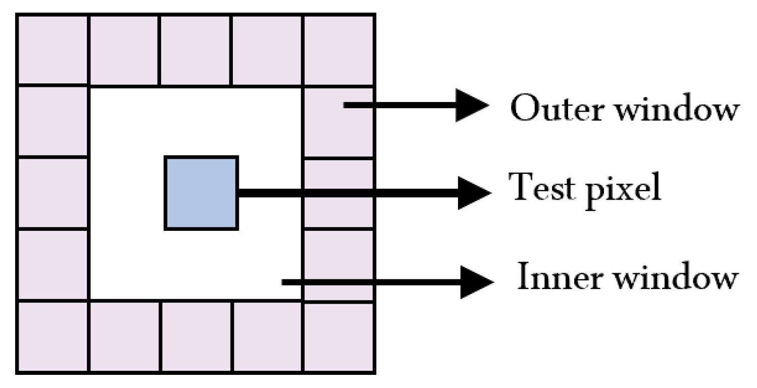
To improve AD accuracy, a multi-directional dual-window RAD detector is designed. This detector fully exploits neighborhood and local background information, significantly improving detection performance by providing a more nuanced analysis of spatial relationships.

(3)

To effectively integrate the spatial and spectral data of HSI and improve the robustness and precision of detection, a saliency weighting strategy is proposed. This strategy is based on the spatial–spectral union, combining the Euclidean distance, spectral gradient, and Spearman correlation coefficient to achieve more precise anomaly discrimination.

2. Materials and Methods

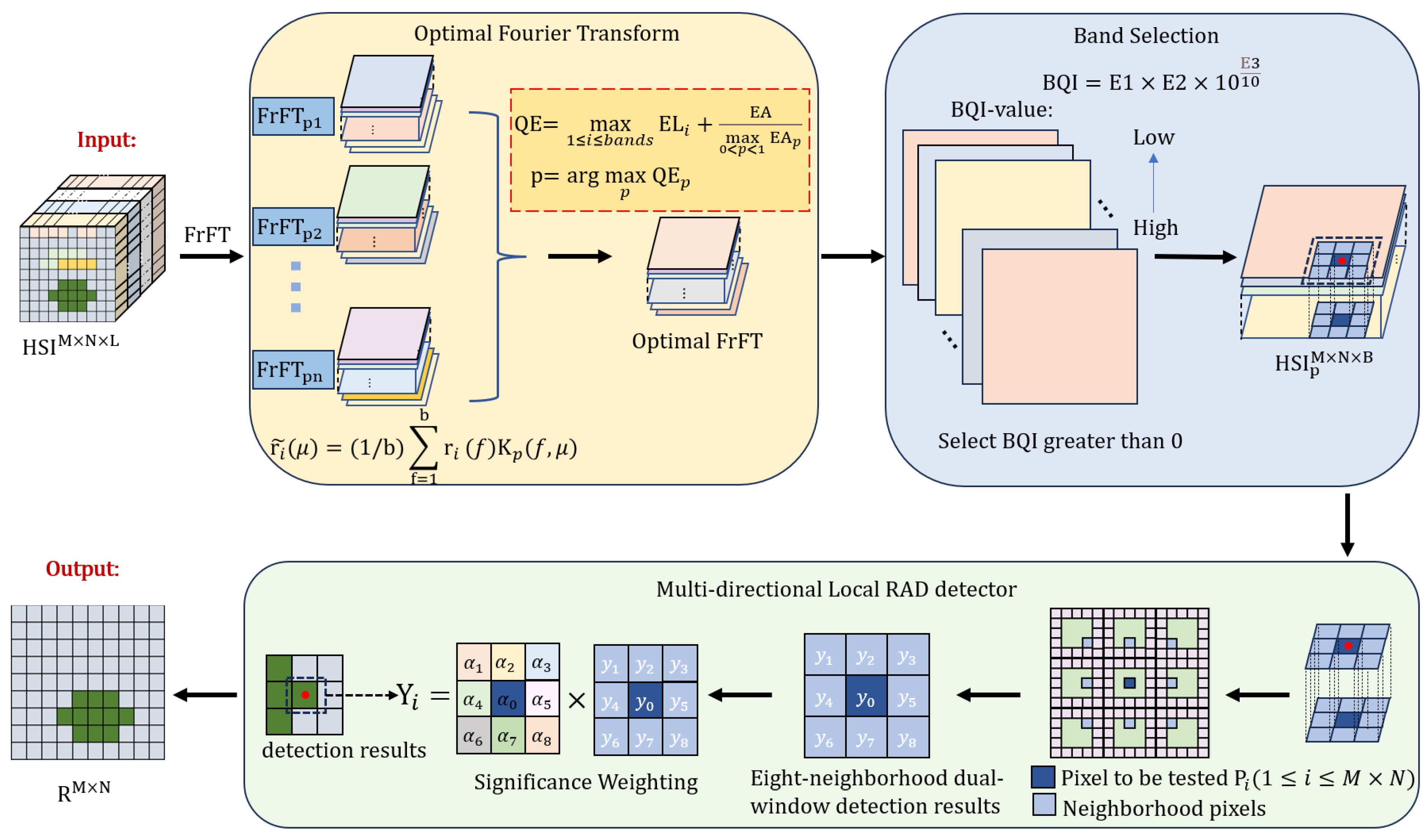
2.1. Overall Framework

The method proposed in this paper comprises three main steps, and the framework diagram of the proposed method is presented in Figure 1. Firstly, the input hyperspectral image ${HSI}^{M\times N\times L}$ undergoes FrFT based on the optimal criterion. By comprehensively considering factors such as entropy, standard deviation, and SNR for both individual bands and the entire image, this paper introduces a new global quality evaluation standard (quality evaluation, QE) to accurately determine the optimal FrFT order $p$. After the optimal FrFT, the HSI retains the maximum amount of information from both the original and Fourier domains, thereby enhancing the separability between anomalies and the background. After the optimal fractional-order Fourier transform, there are significant differences in the amount of information contained in each band. To reduce the computational burden and enhance the detection efficiency, this paper designs a band selection mechanism (entropy-enhanced band selection, EEBS). By evaluating the comprehensive quality (band quality index, BQI) of all bands to rank them, high-quality bands are selected, and bands with lower information content or even redundancy are eliminated, thereby providing an optimized input dataset ${HSI}_p^{M\times N\times B}(0<B<L)$ for subsequent processing. In the AD stage, this paper designs a multi-directional local RAD detector. This detector fully leverages the local background and neighborhood information of the hyperspectral image to construct a multi-directional dual-window structure, enabling more refined detection for each pixel. The pixel to be tested and its eight neighborhood directions (up, down, left, right, up-left, down-left, up-right, down-right) are subjected to local RAD detection. The detection result of each pixel depends not only on its own detection result but also on the detection results of its neighbors. To further optimize the reliability and robustness of the detection results, we also propose a weighted strategy based on the joint spatial–spectral information. Through the significantly weighted summation of the detection results, the in-depth fusion of spatial and spectral information is realized, which remarkably improves the overall detection performance.

2.2. Optimal Fourier Transform

Currently, FrFT is extensively applied in remote sensing. FrFT can be understood as the representation of a signal rotated counterclockwise by any angle on the time axis to the $\mathit{s}$-axis, where the angle is determined by the fractional order $p$ of the transform, and the s-axis is referred to as the fractional Fourier domain. By applying fractional Fourier transforms of various orders, all the characteristics of the signal as it gradually transitions from the time domain to the frequency domain can be obtained, allowing for the inversion of detailed time-frequency characteristics of the signal. Specifically, a test pixel $r_i\in {HSI}^{b\times 1}$ is projected into the fractional domain, and the pixel after FrFT can be expressed as:

$$\widetilde{r_i}\left(\mu \right)=(1/b){\sum }_{f=1}^b{r}_i\left(f\right)K_p\left(f,\mu \right)$$

(1)

$$K_p\left(f,\mu \right)=\left\{\begin{array}{c}{A}_{\mathrm{\varnothing }}\exp \left[j\pi \left(f^2\cot \mathrm{\varnothing }-2fu\csc \mathrm{\varnothing }+{\mu }^2\cot \mathrm{\varnothing }\right)\right],\varnothing \ne n\pi \\ \delta \left(f-\mu \right), \varnothing =2n\pi \\ \delta \left(f+\mu \right), \varnothing =2\left(n+1\right)\pi \end{array}\right.$$

(2)

$$A_{\mathrm{\varnothing }}={\displaystyle \frac{exp [-j\pi \mathrm{sgn}\left(\mathit{sin}\mathrm{\varnothing }\right)/4+j\mathrm{\varnothing }/2]}{{|\mathit{sin}\mathrm{\varnothing }|}^{1/2}}}$$

(3)

where $f$ and $\mu$ represent indexes, $n$ is an arbitrary integer, $p$ is the fractional order of the FrFT, and $\mathbf{\varnothing }=p\times \pi /2$ represents the rotation angle. When $p=0$, $\widetilde{r_i}$ denotes the original spectrum and when $p=1$, $\widetilde{r_i}$ denotes the Fourier transform of the original spectrum. After different fractional order Fourier transforms, the signal contains different time domain information and frequency domain information.

Fractional Fourier entropy was used in the reference [23] to choose the optimal transform order. We select the fractional order $p$, corresponding to the maximum entropy value, by calculating the entropy value for each band of the transformed domain HSI. A higher entropy value indicates better image quality, meaning it is sharper and carries more information. However, a higher entropy value may also suggest excessive noise in the band. Therefore, we consider three indicators—entropy value, standard deviation, and SNR—to measure the quality of the bands. Bands with excessively low standard deviations may contain less information, while bands with high SNR typically contain less noise.

Considering the fact that the optimal fractional order in the reference [23] was chosen to be the order of the band with the highest entropy value, but the bands used for subsequent detection are not just the one with the highest entropy value. Therefore, while we select the single band with the highest quality, we also consider the overall quality of all the bands corresponding to each fractional order. For the FrFT of any order, we calculate the quality of the individual bands at that order (energy level, EL) as well as the quality of the overall bands (energy aggregation, EA):

$$EL={\displaystyle \frac{\left(E2+1\right)E1}{1+e^{-{10}^{\frac{E3}{10}}}}}$$

(4)

$$EA={\sum }_{i=1}^{bands}E1\times E2\times {10}^{{\displaystyle \frac{E3}{10}}}$$

(5)

where $bands$ represent the overall count of bands in the HSI, $E1$ is the entropy value of each band, $E2$ is the standard deviation of each band, and $E3$ is the SNR of each band. The computation of $E1$, $E2$, and $E3$ is shown below:

$$E1=-{\sum }_{i=0}^{L-1}{q}_i\log \left(q_i\right)$$

(6)

$$E2=\sqrt{{\displaystyle \frac{1}{N}}{\sum }_{i=1}^N{(x_i-\mu )}^2}$$

(7)

$$E3=10{\mathit{log}}_{10}\left({\displaystyle \frac{{\mu }^2}{{\sigma }^2}}\right)$$

(8)

where $L$ represents the gray level of the image, $q_i$ is the probability of the ith gray level, $N$ is the total number of pixels in the image, $x_i$ is the value of each pixel, $\mu$ is the mean value of the pixels, and ${\sigma }^2$ is the variance of the noise.

To find the optimal FrFT order, this paper proposes a new image quality evaluation metric (quality evaluation, QE) that comprehensively considers both the single-band quality EL and the overall quality of all bands EA. Based on the balance between local band representativeness and global band performance, this metric is normalized to achieve a fair comparison of image quality at different fractional orders, thus providing a comprehensive assessment of the image quality at various orders. The QE is defined as:

$$QE=\underset{1\le i\le \mathit{bands}}{\mathit{max}}{EL}_i+{\displaystyle \frac{EA}{\underset{0<p<1}{\mathit{max}}{EA}_p}}$$

(9)

Our proposed optimal criterion formula for the FrFT order is as follows:

$$bp=arg \underset{p}{\mathit{max}}{ QE}_p$$

(10)

The $bp$ is the optimal FrFT order we choose, and the hyperspectral image ${HSI}^{M\times N\times L}$ after $bp$ order FrFT is denoted by ${HSI}_p^{M\times N\times L}$.

2.3. Entropy-Enhanced Band Selection

After applying the optimal FrFT, not all bands of the HSI contain rich information. The entropy of an image reflects the average amount of information in the image, the standard deviation of the image can help assess its contrast, and an image with a high SNR typically contains less noise. Therefore, to better evaluate the overall quality of the bands, we multiply these three metrics to ensure the selection of bands that are rich in information, high in contrast, and low in noise, and we redefine a new metric (band quality index, BQI) as follows:

$$BQI=E1\times E2\times {10}^{{\displaystyle \frac{E3}{10}}}$$

(11)

The value of BQI is positive, and a higher BQI indicates better performance in terms of complexity, contrast, and signal clarity, which represents better quality. We calculate the BQI for each band and rank the bands based on their BQI values. Bands with an entropy value of 0 indicate that the image is uniform and does not contain any information. Therefore, we perform band selection on the hyperspectral image to remove these bands with an entropy of 0. The hyperspectral image ${HSI}_p^{M\times N\times B}(0<B<L)$ after band selection will be used for subsequent AD.

HSI often has hundreds of bands, resulting in a massive amount of data, and processing all these bands may require significant computational power. Moreover, some bands may be affected by noise or contain useless information. Compared to traditional band selection techniques, the proposed band selection mechanism operates in the transform domain, enabling more effective retention of key features of both the background and anomalies, thereby significantly improving detection performance. Additionally, this mechanism is not only computationally simple and low in complexity but also efficiently selects high-quality bands and effectively eliminates redundant bands. Selecting a subset of useful bands can reduce computational load and storage requirements, thereby improving the efficiency of image processing [24,25].

2.4. Multi-Directional Local RAD Detector

The scenes in HSI are complex and diverse, with different regions possibly exhibiting distinct spectral characteristics for both background and target pixels. The sliding dual-window anomaly detector [26] can adjust background statistics dynamically, allowing the detection method to adapt to the local characteristics of the image. Figure 2 shows the schematic diagram of the sliding dual window. The sliding dual window comprises an inner window and an outer window, where the inner window contains the pixel to be detected, and the outer window is used to estimate the background information.

Specifically, let $\tilde{X}=[{\tilde{r}}_{i1},{\tilde{r}}_{i2},\dots {\tilde{r}}_{il}]$ denote the surrounding pixels between the outer and inner window, and the algorithm based on the sliding double window can be described as:

$$y_i={{\tilde{r}}_i}^T{R_l}^{-1}{\tilde{r}}_i$$

(12)

$$R_l=({\displaystyle \frac{1}{N}})\tilde{X}{\tilde{X}}^T$$

(13)

$$l=w_{out}\times w_{out}-w_{in}\times w_{in}$$

(14)

where $y_i$ is the detection result of the $i$th pixel, $R_l$ represents the autocorrelation matrix of the local pixel, $l$ represents the number of local background pixels, $w_{out}$ represents the size of the outer window, and $w_{in}$ represents the size of the inner window. Mining local spatial features with two windows of different sizes centered on the test pixel, the region between the outer and inner windows is considered as a pure background pixel, which allows a better estimation of the background information.

However, anomalies usually do not exist in the form of individual pixels but appear as irregular regions. Using a dual-window detector centered only on the pixel to be measured may contain some anomalous information, leading to errors in judgment. Considering the spatial structure of the anomalous pixel, its neighborhood information should also be taken into account when detecting the pixel to be tested. It is generally believed that two spatially close pixels are closer to the same substance. In reference [27], a dispersion-direction CEM target detector is designed, which utilizes spatial information from eight adjacent neighborhoods surrounding each pixel to boost the accuracy of target identification.

Motivated by this, we introduce eight-neighborhood information on the traditional sliding double-window AD algorithm, which enables the new detector to synthesize more spatial information in the local space. The model of the multi-directional local RAD detector is shown in Figure 3. The eight-neighborhood method can capture the spatial correlation between the pixels and has better adaptability to regions with large local variations. Moreover, by combining the neighborhood information, some isolated noise pixels are comprehensively analyzed together with the surrounding pixels, which helps to suppress the false alarms of single-point noise.

The eight-neighborhood dual-window anomaly detector not only detects individual pixels but also takes into account the eight adjacent points of each pixel (namely, top, bottom, left, right, top-right, bottom-right, top-left, and bottom-left). The double-window RAD detection results centered on the pixel ${{\tilde{\mathit{r}}}_{\mathit{i}}}_{(\mathit{x},\mathit{y})}$ to be measured, as well as those centered on ${{\tilde{r}}_i}_{(x-1,y)}$, ${{\tilde{r}}_i}_{(x,y-1)}$, ${{\tilde{r}}_i}_{(x-1,y-1)}$, ${{\tilde{r}}_i}_{(x+1,y)}$, ${{\tilde{r}}_i}_{(x,y+1)}$, ${{\tilde{r}}_i}_{(x+1,y+1)}$, ${{\tilde{r}}_i}_{(x-1,y+1)}$, ${{\tilde{r}}_i}_{(x+1,y-1)}$, respectively, are computed. Multi-directional detection can also reduce the misjudgment caused by the mixed information of a single direction and thus can better describe the pixel to be detected. Therefore, when we detect the pixel to be measured, in addition to the local detection results of the pixel to be measured, we also get the detection results of eight directions, as shown in the following equation:

$$\mathit{R}=\left[\begin{array}{ccc}{y}_{\left(i-1,j-1\right)}& y_{\left(i-1,j\right)}& y_{\left(i-1,j+1\right)}\\ y_{\left(i,j-1\right)}& y_{\left(i,j\right)}& y_{\left(i,j+1\right)}\\ y_{\left(i+1,j-1\right)}& y_{\left(i+1,j\right)}& y_{\left(i+1,j+1\right)}\end{array}\right]$$

(15)

where $\mathit{R}$ denotes the initial detection result of the to-be-tested center pixel after multi-directional dual-window detection, $y_{(i,j)}$ denotes the result of the to-be-tested pixel after the sliding dual-window anomaly detector, $y_{\left(i-1,j-1\right)}$, $y_{\left(i-1,j\right)}$, $y_{\left(i-1,j+1\right)}$, $y_{(i,j-1)}$, $y_{\left(i,j+1\right)}$, $y_{\left(i+1,j-1\right)}$, $y_{\left(i+1,j\right)}$ and $y_{\left(i+1,j+1\right)}$ are the results of the neighboring pixels of the pixel to be measured after the sliding double window anomaly detector.

To fully consider the individual influence of each direction on the central pixel, we give different weights to the detection results of each direction according to the combination of Euclidean distance, Spearman correlation coefficient, and cosine of spectral gradient. Combining these three similarity measures can make the detection results more robust and accurate. In the spectral dimension, we consider the Spearman correlation coefficient and the cosine of the spectral gradient between the pixel that needs to be measured and the neighboring pixels. The Spearman correlation coefficient [28] measures the rank correlation of two spectral vectors and is suitable for comparing the shape changes of spectral curves. The Spearman correlation coefficient $\rho$ is calculated as follows:

$$\rho ={\displaystyle \frac{cov\left(x_p,x_q\right)}{\sqrt{var\left(x_p\right)var\left(x_q\right)}}}$$

(16)

where $cov$ denotes covariance and $var$ denotes standard deviation, $x_p$ and $x_q$ represent the spectral vectors of two pixels, respectively. If the spectral curve shapes of two pixels are similar, the Spearman correlation coefficient approaches 1; if the shapes are opposite, it approaches −1. Spectral gradient has the advantage of highlighting changes in local spectral features and can sensitively capture the slope change of the spectral curve [29]. In practice, the spectral gradient can avoid misjudgments due to light intensity differences. For any two pixels $p$ and $q$, the spectral gradient is calculated as:

$$SG\left(p\right)=(x_{p2}-x_{p1},x_{p3}-x_{p2},\dots ,x_{pbands}-x_{pbands-1})$$

(17)

$$SG\left(q\right)=(x_{q2}-x_{q1},x_{q3}-x_{q2},\dots ,x_{qbands}-x_{qbands-1})$$

(18)

where $x_{pi}$ denotes the value of pixel $p$ in the i-th band. The spectral gradient reflects the rate of spectral change between adjacent bands. Areas with a large spectral gradient may correspond to abrupt change points on the spectral curve, which could potentially indicate anomalous features. The cosine value of the spectral gradient (SGA) is used to measure the similarity between the spectral gradients of two pixels. When the directions of the spectral gradient vectors of two pixels are closer, their cosine value is larger, indicating a higher degree of similarity. According to the spectral gradient of two pixels, the cosine value of their spectral gradient can be calculated by the following formula:

$$SGA\left(p,q\right)=\mathit{cos}{\displaystyle \frac{SG\left(p\right)·SG\left(q\right)}{\parallel SG\left(p\right)\parallel \parallel SG\left(q\right)\parallel }}$$

(19)

where $SG$ is the gradient vector of spectrum, $·$ is the dot product of two vectors and $\parallel SG\left(q\right)\parallel$ is the module of $SG\left(q\right)$. The cosine value of spectral gradient is normalized to obtain the following formula:

$$S\left(p,q\right)={\displaystyle \frac{SGA\left(p,q\right)}{\sum _{q\in Q}SGA\left(p,q\right)}}$$

(20)

where $Q$ is the set of eight neighboring pixels of the central pixel $p$.

In space, the closer a neighboring pixel is to the pixel under test, the greater its contribution to the detection result in that direction should be. In eight-neighborhood detection, different weights are assigned to different directions, with a weight of $1$ for horizontal and vertical directions and a weight of $\sqrt{2}$ for diagonal directions. This paper fully integrates the spatial and spectral information of HSI, combining Euclidean distance, spectral gradient, and Spearman correlation coefficient, to propose a saliency-weighted strategy based on the joint use of spatial and spectral information. For the pixel under test located at a specific position $(i,j)$, the corresponding weight matrix $\mathit{W}$ is defined as:

$$\mathit{W}=\left[\begin{array}{ccc}{\displaystyle \frac{{\rho }_{(i-1,j-1)}}{\sqrt{2}}}{S}_{(i-1,j-1)}& {\rho }_{(i-1,j)}{S}_{(i-1,j)}& {\displaystyle \frac{{\rho }_{(i-1,j+1)}}{\sqrt{2}}}{S}_{(i-1,j+1)}\\ {\rho }_{(i,j-1)}{S}_{(i,j-1)}& 1& {\rho }_{(i,j+1)}{S}_{(i,j+1)}\\ {\displaystyle \frac{{\rho }_{(i+1,j-1)}}{\sqrt{2}}}{S}_{(i+1,j-1)}& {\rho }_{(i+1,j)}{S}_{(i+1,j)}& {\displaystyle \frac{{\rho }_{(i+1,j+1)}}{\sqrt{2}}}{S}_{(i+1,j+1)}\end{array}\right]$$

(21)

When the weight matrix is applied to the initial detection results, the detection results $\mathit{Y}$ of the pixel to be tested will be presented in the form of a $3\times 3$ size matrix:

$$\mathit{Y}=\mathit{R}⨀\mathit{W}=\left[\begin{array}{ccc}{y}_{\left(i-1,j-1\right)}{\displaystyle \frac{{\rho }_{(i-1,j-1)}}{\sqrt{2}}}{S}_{(i-1,j-1)}& {y_{\left(i-1,j\right)}\rho }_{(i-1,j)}{S}_{(i-1,j)}& y_{\left(i-1,j+1\right)}{\displaystyle \frac{{\rho }_{(i-1,j+1)}}{\sqrt{2}}}{S}_{(i-1,j+1)}\\ {y_{\left(i,j-1\right)}\rho }_{(i,j-1)}{S}_{(i,j-1)}& y_{\left(i,j\right)}& y_{\left(i,j+1\right)}{\rho }_{(i,j+1)}{S}_{(i,j+1)}\\ y_{\left(i+1,j-1\right)}{\displaystyle \frac{{\rho }_{(i+1,j-1)}}{\sqrt{2}}}{S}_{(i+1,j-1)}& {y_{\left(i+1,j\right)}\rho }_{(i+1,j)}{S}_{(i+1,j)}& y_{\left(i+1,j+1\right)}{\displaystyle \frac{{\rho }_{(i+1,j+1)}}{\sqrt{2}}}{S}_{(i+1,j+1)}\end{array}\right]$$

(22)

where $⨀$ means Hadma product. To effectively extract spatial data within the local area, the detection result of the central pixel to be measured and the detection results of its neighborhood pixels are summed and averaged. Therefore, for the pixel to be tested at position $(i,j)$, the final detection result of its multi-direction dual-window anomaly detector is as follows:

$$\begin{gathered} Y_{final}{ = y}_{\left(i,j\right)}+{\rho }_{\left(i,j-1\right)}{S}_{\left(i,j-1\right)}{y}_{\left(i,j-1\right)}+{\rho }_{\left(i,j+1\right)}{S}_{\left(i,j+1\right)}{y}_{\left(i,j+1\right)}+{\rho }_{(i-1,j)}{S}_{(i-1,j)}{y}_{(i-1,j)}+ \\ {\rho }_{(i+1,j)}{S}_{(i+1,j)}{y}_{(i+1,j)}+{\displaystyle \frac{{\rho }_{(i-1,j-1)}}{\sqrt{2}}}{S}_{(i-1,j-1)}{y}_{(i-1,j-1)}+{\displaystyle \frac{{\rho }_{(i-1,j+1)}}{\sqrt{2}}}{S}_{(i-1,j+1)}{y}_{(i-1,j+1)}+ \\ {\displaystyle \frac{{\rho }_{(i+1,j-1)}}{\sqrt{2}}}{S}_{(i+1,j-1)}{y}_{(i+1,j-1)}+{\displaystyle \frac{{\rho }_{(i+1,j+1)}}{\sqrt{2}}}{S}_{(i+1,j+1)}{y}_{(i+1,j+1)} \end{gathered}$$

(23)

3. Experimental Analysis

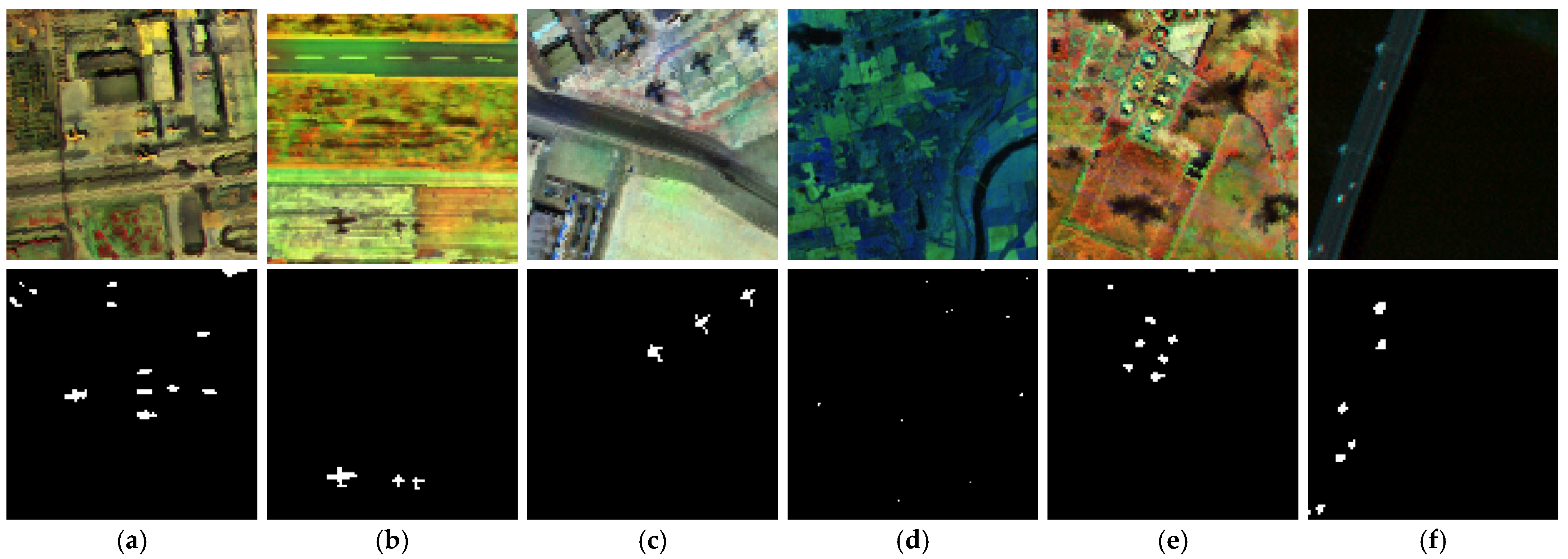
3.1. Hyperspectral Datasets

The datasets utilized in this study represent classic and publicly available resources within the field of hyperspectral target analysis [30,31]. Figure 4 presents the false-color imagery alongside the ground truth maps for the six datasets. The Los Angeles dataset was gathered using AVIRIS sensors over the downtown area of Los Angeles. It features 205 bands at a 7.1 m spatial resolution. Choose a 100 × 100 pixel sub-scene for AD. The Gulfport dataset, gathered using the Airborne Visible/Infrared Imaging Spectrometer (AVIRIS), covers the Gulfport Airport region in Mississippi, USA. It comprises 191 spectral bands spanning wavelengths from 550 to 1850 nm, with a spatial resolution of 3.4 m. For AD, a 100 × 100 pixel subset was extracted, featuring a mix of airport runways, highways, and sparse vegetation. Similarly, the San Diego dataset, also captured by AVIRIS, focuses on San Diego Airport in California. This dataset consists of 189 bands and a spatial resolution of 3.5 m, with a 100 × 100 pixel subset designated for AD analysis. The Hyperion dataset, acquired via the Hyperion imaging sensor, was refined by eliminating bands with low signal-to-noise ratios (SNRs) and those lacking calibration, leaving 155 usable bands. A 150 × 150 pixel sub-image, accompanied by a ground truth map, was employed to scrutinize anomalous points. Meanwhile, the Texas Coast dataset, collected by AVIRIS in 2010 along the Texas coastline, includes 204 bands but has a coarser spatial resolution of 17.2 m. A 100 × 100 pixel subset was chosen for AD, presenting a relatively straightforward background despite its lower resolution. Lastly, the Pavia dataset originates from the ROSIS airborne imaging spectrometer, deployed during flights over northern Italy. It features 102 bands with a sharp geometric resolution of 1.3 m. A 100 × 100 pixel subset was selected for AD, showcasing a backdrop of water and bridges, interspersed with anomalies such as vehicles.

3.2. Experimental Design

To assess the efficacy and advantage of the proposed method, we conduct experiments on six classical HSI datasets. We compared the proposed method with various classical and state-of-the-art algorithms, including RAD [32], FrFE-RX, FEBPAD [33], SFBA-AD [34], and SSFAD [35]. RAD is an AD algorithm based on a correlation matrix, which simplifies the RXD operations without compromising detection performance. The FrFE-RX algorithm based on FrFT enhances the separation between anomalies and the background. FEBPAD combines FrFT and low-rank sparse matrix decomposition to separate anomalies from background and noise. SFBA-AD proposes a spatial–spectral anomaly scoring strategy through sub-feature grouping and binary accumulation, which further improves the algorithm’s robustness. SSFAD is an AD algorithm based on FrFT and weighted cooperative representation. In all experiments, the area under the receiver operating characteristic curve (AUC) [36] was used as a quantitative metric to evaluate detection performance. To emphasize the advantages of each method, the optimal AUC values obtained by each method are marked in bold in the table. All experiments were conducted on a PC equipped with a 12th Gen Intel(R) Core(TM) i7-12700 CPU running at a base speed of 2.10 GHz, with 16 GB of RAM. The experimental platform used was MATLAB R2022b 1.8.0_202.

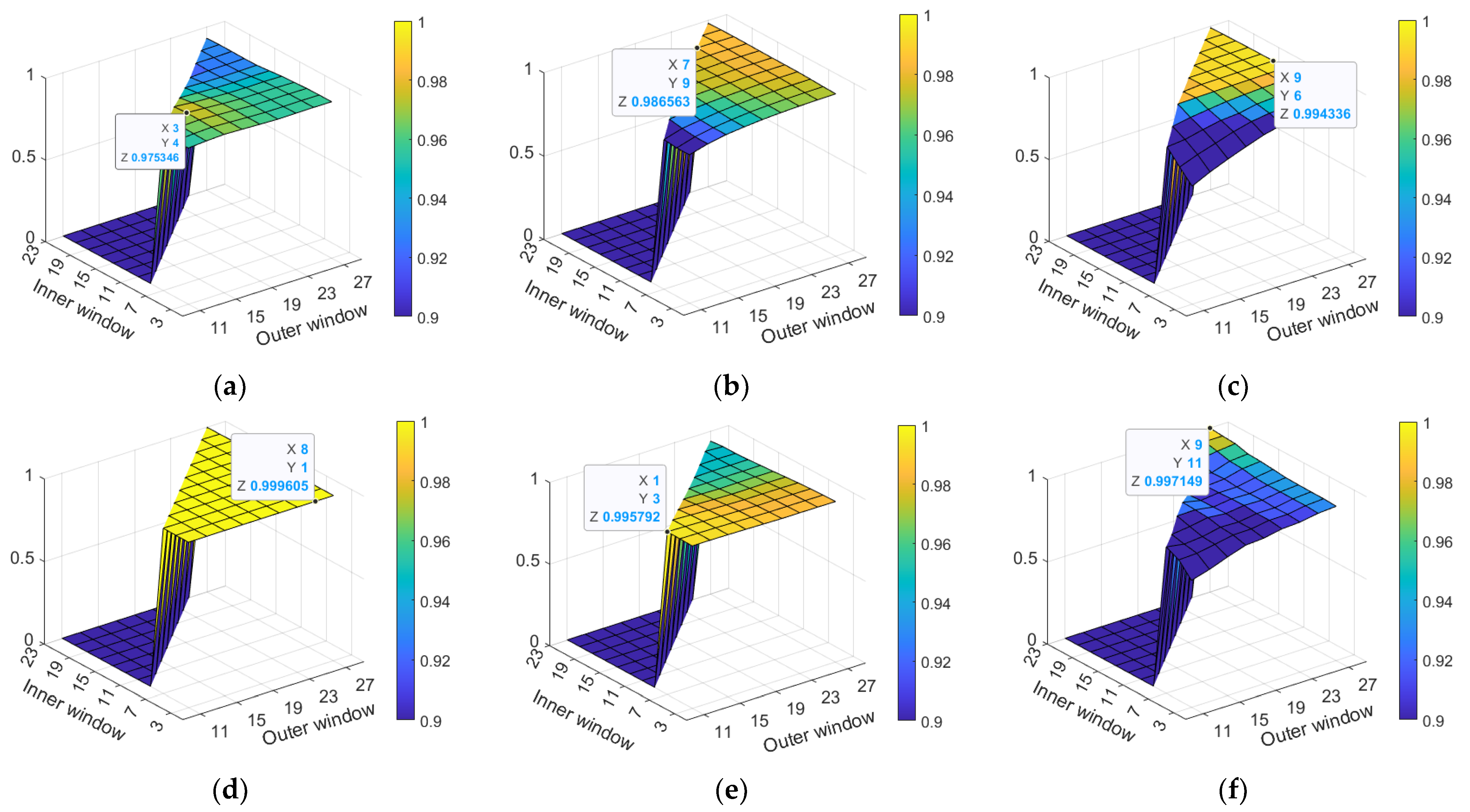
3.3. Parameter Analysis

The detection performance (measured by AUC value) of the proposed approach varies with the selection of the inner and outer window sizes. The larger outer window $w_{out}$ helps to capture the background information, so the $w_{out}$ size range is set to $11\le w_{out}\le 27$ for the parametric analysis. The proper size of the inner window can accurately locate the anomaly pixel, so the size range is set to $3\le w_{in}\le w_{out}-4$. Figure 5 shows the effect of different combinations of inner and outer window sizes on model detection performance. Experimental results show that the optimal window size combinations of different datasets are different, but they all reflect the efficiency and robustness of the proposed method. In the Los Angeles dataset, the detection performance is the best with an AUC value of 0.9753 when the outer and inner window size is (15, 9). In the Gulfport dataset, the detection performance is the best with an AUC value of 0.9866 when the outer and inner window size is (23, 19). In the San Diego dataset, when the outer and inner window size is (27, 13), the detection accuracy reaches the peak, and its AUC value is 0.9943. In the Hyperion dataset, when the outer and inner window size is (25, 3), the detection accuracy is the best, and its AUC score is as high as 0.9996. In the Texas Coast dataset, when the outer and inner window size is (11, 7), the detection accuracy is the highest, and its AUC value is 0.9957. In the Pavia dataset, when the size of the outer and inner window is (27, 23), the detection accuracy is the highest, and the AUC value is 0.9971. Experimental results show that the size of the window affects the separation of anomaly and background. Specifically, the range for the outer window size $11\le w_{out}\le 27$ is designed to strike a balance between capturing sufficient background information and avoiding excessive computational overhead. Meanwhile, the range for the inner window size $3\le w_{in}\le w_{out}-4$ is chosen to achieve an optimal trade-off between accurately localizing anomaly pixels and preventing background contamination. These parameter ranges were determined through extensive experimental validation to ensure their effectiveness and robustness across various scenarios. To further improve the detection performance, the inter and outer window sizes can be optimized in practical applications according to the proportion of anomaly pixels and the characteristics of the dataset. This parameter adjustment strategy can effectively enhance the adaptability and detection precision of the proposed approach so as to meet the application requirements of different scenarios.

3.4. Detection Performance

To achieve the best detection performance, we adjust the size of double window according to the characteristics of different datasets: for the Los Angeles dataset, the double window size is configured as (15, 9); for the Gulfport dataset, the double window size is configured as (23, 19); for the San Diego dataset, the double window size is configured as (27, 13); for the Hyperion dataset, the double window size is configured as (25, 3); for the Texas Coast dataset, the double window size is configured as (11, 7); for the Pavia dataset, the double window size is configured as (27, 23).

To visually contrast the detection performances of the six methods, Figure 6 displays the detection results of the six methods on six datasets. From the visual effect, the proposed method detects anomalies on all six datasets and significantly improves the ability to separate anomalies from the background. However, RAD, FrFE-RX, and FEBPAD are not prominent enough to detect anomalies in the Los Angeles dataset, Gulfport dataset, San Diego dataset, Hyperion dataset, and it is difficult to effectively distinguish anomalies from the background. In the Texas Coast dataset, some background pixels, except for abnormal pixels, are detected by the three algorithms, so the background and anomaly cannot be separated effectively. Although SFBA-AD can detect abnormal pixels in six datasets, its ability to suppress background is weak, and the separability between background and anomaly is insufficient. Its detection results contain numerous background pixels other than the anomalies, showing low background suppression ability. SSFAD can basically detect the abnormal pixels, but the background suppression capability falls short of the proposed method, and the background or noise other than anomalies still is mistakenly detected. For the Pavia dataset, SFBA-AD has poor background suppression ability. Moreover, the visual effect shows that SSFAD can not completely detect all abnormal pixels, and the detection performance is not significant enough. The proposed method shows excellent detection performance on all datasets, which can not only clearly separate anomalies from the background, but also effectively suppress the background. In the case of the Pavia dataset and others with complex backgrounds, this method successfully identifies all anomalies, significantly suppresses the background and noise, and the detection results are visually clearer. The proposed methods, FrFE-RX and FEBPAD, are all detected in the fractional Fourier domain, so the background and anomaly are effectively separated. In addition, this method further combines multi-directional neighborhood information and makes full use of the spatial and spectral characteristics of HSI. This fusion not only enhances the separation degree between anomaly and background but also improves the overall detection accuracy.

For better quantitative analysis, we calculate the AUC values of the detection results of different methods on six different datasets, as shown in

Table 1. AUC of detection results on Los Angeles dataset (Bold data in the table are optimal auc values).

Method	AUC(D,F)	AUC(D,τ)	AUC(F,τ)	AUCTD	AUCBS	AUCTDBS	AUCODP	AUCSNPR
RAD	0.8180	0.0998	0.0442	0.9178	0.7738	0.0556	1.0556	2.2579
FrFE-RX	0.8836	0.0439	0.0164	0.9275	0.8672	0.0275	1.0275	2.6768
FEBPAD	0.9092	0.0181	0.0079	0.9273	0.9013	0.0102	1.0102	2.2911
SFBA-AD	0.7639	0.3002	0.0983	1.0641	0.6656	0.2019	1.2019	3.0539
SSFAD	0.9518	0.2852	0.0524	1.2370	0.8994	0.2328	1.2328	5.4427
proposed	0.9753	0.1299	0.0149	1.1052	0.9604	0.1150	1.1150	8.7181

,

Table 2. AUC of detection results on Gulfport dataset (Bold data in the table are optimal auc values).

Method	AUC(D,F)	AUC(D,τ)	AUC(F,τ)	AUCTD	AUCBS	AUCTDBS	AUCODP	AUCSNPR
RAD	0.9519	0.0707	0.0250	1.0226	0.9269	0.0457	1.0457	2.8280
FrFE-RX	0.9790	0.1319	0.0209	1.1109	0.9581	0.1110	1.1110	6.3110
FEBPAD	0.9631	0.0953	0.0226	1.0584	0.9405	0.0727	1.0727	4.2168
SFBA-AD	0.9758	0.7917	0.1019	1.7675	0.8739	0.6898	1.6898	7.7694
SSFAD	0.9781	0.4584	0.0388	1.4365	0.9393	0.4196	1.4196	11.8144
proposed	0.9866	0.2927	0.0165	1.2793	0.9701	0.2762	1.2762	17.7394

,

Table 3. AUC of detection results on San Diego dataset (Bold data in the table are optimal auc values).

Method	AUC(D,F)	AUC(D,τ)	AUC(F,τ)	AUCTD	AUCBS	AUCTDBS	AUCODP	AUCSNPR
RAD	0.8632	0.0655	0.0381	0.9287	0.8251	0.0274	1.0274	1.7192
FrFE-RX	0.9660	0.0880	0.0196	1.0540	0.9464	0.0684	1.0684	4.4898
FEBPAD	0.9766	0.1327	0.0266	1.1093	0.9500	0.1061	1.1061	4.9887
SFBA-AD	0.9837	0.7506	0.0827	1.7343	0.9010	0.6679	1.6679	9.0762
SSFAD	0.9829	0.3345	0.0358	1.3174	0.9471	0.2987	1.2987	9.3436
proposed	0.9943	0.3737	0.0487	1.3680	0.9456	0.3250	1.3250	7.6735

,

Table 4. AUC of detection results on Hyperion dataset (Bold data in the table are optimal auc values).

Method	AUC(D,F)	AUC(D,τ)	AUC(F,τ)	AUCTD	AUCBS	AUCTDBS	AUCODP	AUCSNPR
RAD	0.9969	0.2165	0.0404	1.2134	0.9565	0.1761	1.1761	5.3589
FrFE-RX	0.9953	0.2331	0.0327	1.2284	0.9626	0.2004	1.2004	7.1284
FEBPAD	0.9927	0.1624	0.0197	1.1551	0.9730	0.1427	1.1427	8.2437
SFBA-AD	0.9362	0.5882	0.1260	1.5244	0.8102	0.4622	1.4622	4.6683
SSFAD	0.9790	0.2322	0.0241	1.2112	0.9549	0.2081	1.2081	9.6349
proposed	0.9996	0.1896	0.0037	1.1892	0.9959	0.1859	1.1859	51.2432

,

Table 5. AUC of detection results on Texas Coast dataset (Bold data in the table are optimal auc values).

Method	AUC(D,F)	AUC(D,τ)	AUC(F,τ)	AUCTD	AUCBS	AUCTDBS	AUCODP	AUCSNPR
RAD	0.9904	0.3240	0.0587	1.3144	0.9317	0.2653	1.2653	5.5196
FrFE-RX	0.9891	0.3001	0.0426	1.2892	0.9465	0.2575	1.2575	7.0446
FEBPAD	0.9820	0.3356	0.0106	1.3176	0.9714	0.3250	1.3250	31.6604
SFBA-AD	0.9591	0.8547	0.1463	1.8138	0.8128	0.7084	1.7084	5.8421
SSFAD	0.9951	0.4341	0.0352	1.4292	0.9599	0.3989	1.3989	12.3324
proposed	0.9957	0.1972	0.0600	1.1929	0.9357	0.1372	1.1372	3.2867

and

Table 6. AUC of detection results on Pavia dataset (Bold data in the table are optimal auc values).

Method	AUC(D,F)	AUC(D,τ)	AUC(F,τ)	AUCTD	AUCBS	AUCTDBS	AUCODP	AUCSNPR
RAD	0.9934	0.1604	0.0297	1.1538	0.9637	0.1307	1.1307	5.4007
FrFE-RX	0.9868	0.1812	0.0264	1.1680	0.9604	0.1548	1.1548	6.8636
FEBPAD	0.9840	0.1090	0.0025	1.0930	0.9815	0.1065	1.1065	43.6000
SFBA-AD	0.9921	0.9211	0.0872	1.9132	0.9049	0.8339	1.8339	10.5631
SSFAD	0.9960	0.1793	0.0041	1.1753	0.9819	0.1652	1.1652	12.7168
proposed	0.9971	0.2395	0.0141	1.2366	0.9930	0.2354	1.2354	58.4146

. Table 1 shows that the AUC(D,F) of the proposed approach is the highest among the six methods, and its value reaches 0.9753, which is 9.4% higher than FrFE-RX. The AUC_BS and AUC_SNPR values of our proposed approach are also the highest, which shows that the method has better background suppression. Table 2 reveals that the suggested method reaches the highest AUC(D,F) of 0.9866 when compared to the other five methods. The AUC(D,τ) of SFBA-AD is the highest, reaching 0.7917, but its AUC(F,τ) value is also the highest. SFBA-AD exhibits the poorest background noise reduction compared to the other five approaches. It is not difficult to find that the AUC(F,τ), AUC_BS and AUC_SNPR values of the proposed method are the highest, which indicates that the performance of this method in background suppression is excellent. Table 3 shows the AUC values on the San Diego dataset. The AUC(D,F) value of the method we propose is 0.9943, which is the highest among the six methods. Compared with the traditional RAD method, the AUC(D,F) increased by 15.19%. The AUC(D,τ) of SFBA-AD is the highest; however, its capacity for background suppression is the lowest. The detection results of different methods on the Hyperion dataset are given in Table 4, which shows that the proposed method exhibits the optimal detection performance. The proposed method demonstrates superior background suppression efficacy, and its AUC_SNPR value reaches 51.2432. Compared with SFBA-AD, the AUC(D,F) of the proposed method is increased by nearly 6.8%. Table 5 illustrates that our proposed method maintains outstanding detection performance on the Texas Coast dataset. The AUC(D,F) of the proposed method is the highest, reaching 0.9957, which is nearly 3.8% higher than that of SFBA-AD. However, FEBPAD has the best performance in background suppression. Table 6 shows the detection results on the Pavia dataset, and we can see that the AUC(D,F) value of the proposed method is the highest, reaching 0.9971. And the background suppression performance is also the best. FEBPAD has the worst detection performance, which may be due to its insufficient integration of spectral and spatial information, and its detection performance is limited in complex background scenes. From the six tables, we can see that our proposed method shows superior detection performance on six datasets, and all of them are higher than other comparison algorithms.

3.5. Ablation Experiment

To verify the effectiveness of selecting the FrFT order using the optimal criterion proposed in this paper, we conduct a comparative experiment with FrFE-RX. To eliminate the influence of other factors, we maintain the same experimental setup except for the different methods in selecting the transform order. FrFEBP-RX utilizes the optimal criterion proposed in this paper to select the optimal FrFT order $p_1$, and then carries out RXD detection on HSI passing through $p_1$ order Fourier transform. FrFE-RX utilizes the fractional Fourier entropy proposed in reference [29] to select the optimal FrFT order $p_2$, and then carries out RXD detection on HSI passing through $p_2$ order Fourier transform. Figure 7 intuitively compares the results of both methods on six datasets.

As seen from Figure 7, FrFEBP-RX is more accurate in detecting anomalies than FrFE-RX. On the Los Angeles dataset, FrFE-RX can hardly see the shape and location of anomalies, while FrFEBP-RX can clearly distinguish background from anomalies. On the other five datasets, although FrFE-RX detects anomalies to some extent, it is not as prominent as FrFEBP-RX, which shows that FrFEBP-RX has better AD performance. As illustrated in

Table 7. AUC of detection results of two methods on six datasets.

Dataset	Method	AUC(D,F)	AUC(D,τ)	AUC(F,τ)	AUCTD	AUCBS	AUCTDBS	AUCODP	AUCSNPR
Los Angeles	FrFE-RX	0.8836	0.0439	0.0164	0.9275	0.8672	0.0275	1.0275	2.6768
	FrFEBP-RX	0.8960	0.0406	0.0130	0.9366	0.8830	0.0276	1.0276	3.1231
Gulfport	FrFE-RX	0.9790	0.1319	0.0209	1.1109	0.9581	0.1110	1.1110	6.3110
	FrFEBP-RX	0.9671	0.0796	0.0185	1.0467	0.9486	0.0611	1.0611	4.3027
San Diego	FrFE-RX	0.9660	0.0880	0.0196	1.0540	0.9464	0.0684	1.0684	4.4898
	FrFEBP-RX	0.9678	0.0597	0.0219	1.0275	0.9459	0.0378	1.0378	2.7260
Hyperion	FrFE-RX	0.9953	0.2331	0.0327	1.2284	0.9626	0.2004	1.2004	7.1284
	FrFEBP-RX	0.9976	0.2084	0.0258	1.2060	0.9718	0.1826	1.1826	8.0775
Texas Coast	FrFE-RX	0.9891	0.3001	0.0426	1.2892	0.9465	0.2575	1.2575	7.0446
	FrFEBP-RX	0.9903	0.2903	0.0442	1.2806	0.9461	0.2461	1.2461	6.5679
Pavia	FrFE-RX	0.9868	0.1812	0.0264	1.1680	0.9604	0.1548	1.1548	6.8636
	FrFEBP-RX	0.9893	0.2520	0.0257	1.2413	0.9636	0.2263	1.2263	9.8054

, to evaluate the detection capability of the two methods more accurately, we compare the AUC scores for the detection outcomes of FrFE-RX and FrFEBP-RX on six datasets. We find that the AD performance of FrFEBP-RX is better than that of FrFE-RX. On the Los Angeles dataset, the AUC(D,F) of FrFEBP-RX is 0.8960, which is 1.4% higher than that of FrFEBP-RX, and the values of AUC_TD, AUC_BS, AUC_TDBS, AUC_ODP, and AUC_SNPR of FrFEBP-RX are higher than those of FrFE-RX, which indicates that FrFEBP-RX has better target identification and background suppression ability. On the Gulfport dataset, while the AUC(D,F) of FrFEBP-RX is inferior to that of FrFE-RX, the AUC(F,τ) of FrFEBP-RX is lower than that of FrFE-RX. On the San Diego and Texas Coast datasets, the AUC(D,F) of FrFEBP-RX is 0.9678 and 0.9903, respectively, which are higher than those of FrFE-RX. For the Hyperion and Pavia datasets, the AUC(D,F) and AUC_SNPR of FrFEBP-RX are higher than those of FrFE-RX, and the AUC_SNPR of FrFEBP-RX in Pavia is 9.8054, which is 42.86% higher than that of FrFE-RX. To sum up, the optimal criterion proposed in this paper to select the optimal FrFT is effective and can improve the accuracy of AD.

For the HSI processed by the optimal FrFT, not all bands contain abundant information. Figure 8 shows the entropy values of each band in the Hyperion dataset after applying the 0.1-order FrFT. The dataset consists of 155 bands, and the entropy values of bands beyond the 120th are significantly lower. This phenomenon may be related to the energy redistribution characteristics of the FrFT: FrFT redistributes the energy of the signal between the time and frequency domains, and the 0.1-order transform may reduce the energy concentration of certain bands, thereby decreasing their entropy values. Additionally, these bands may inherently contain less information or be affected by noise and sensor errors, further contributing to the reduction in entropy values. As seen from Figure 8, many bands have an entropy value of 0, indicating that all pixels in these bands have identical values and therefore contain no useful information. Since HSI often consists of hundreds of bands, issues such as high band redundancy and poor band quality arise. In this experiment, an entropy-enhanced band selection mechanism (EEBS) is applied to the transformed images to select bands with higher quality and eliminate those with low or redundant information. This process not only improves detection efficiency but also significantly reduces the computational burden.

4. Discussion

Based on the above analysis, it can be concluded that the algorithm we propose exhibits outstanding performance in hyperspectral anomaly detection. The optimality of the proposed FrFT is validated through the following two aspects: First, we introduced a new global quality evaluation criterion, QE, which comprehensively considers the entropy, standard deviation, and SNR of each band. By maximizing the QE metric, the optimal fractional order can be selected, thereby best preserving the information from both the original data and the Fourier domain. Second, we conducted experimental validation on multiple classic hyperspectral datasets. The results demonstrate that the selected fractional order significantly enhances the separability between anomalies and the background, thereby improving detection performance. By taking a close look at the data in the experimental result table, we can further conduct a comparative analysis of the advantages and disadvantages of each algorithm. FrFE-RX is an anomaly detection method utilizing the fractional Fourier transform. Compared with the traditional RAD anomaly detector, it shows significantly better detection results on the Los Angeles, Gulfport, and San Diego datasets. This suggests that the fractional Fourier transform significantly improves the differentiation of anomalies from the background in these datasets. However, on the Hyperion, Texas Coast, and Pavia datasets, the detection performance of FrFE-RX is inferior to that of RAD. This might be related to its insufficient utilization of spatial information and lack of adaptability to the characteristics of specific datasets. RAD is an anomaly detection algorithm based on the correlation matrix. While it is computationally simple, it exhibits poor adaptability to complex backgrounds, and its performance on the Los Angeles, Gulfport, and San Diego datasets is inferior to that of other comparative algorithms. Although the FrFE-RX method performs detection in the transform domain, its performance on certain datasets is even worse than that of RAD. This indicates that the fractional order selected by FrFE-RX is not optimal, and the method suffers from significant robustness issues. FrFE-RX prioritizes fractional Fourier transform orders by assessing Fourier entropy within a single band, ignoring the overall information of the image. This locally optimized strategy may lead to the failure to fully utilize all the advantages of the FrFT. Especially when dealing with complex and changeable remote-sensing images, it fails to comprehensively capture the overall features of the image, thus limiting the further improvement of anomaly detection performance. Consequently, the detection capability of FrFE-RX is inferior to that of the algorithm introduced in this paper. The SFBA-AD method has the lowest detection effect among all methods on the Los Angeles, Hyperion, and Texas Coast datasets. Its detection results contain a large number of background pixels other than the targets. This may be due to its insufficient ability to suppress the background during the detection process, resulting in a limited contrast between anomalies and the background. SSFAD conducts anomaly detection in the original domain, and the distinction between the background and anomalies is poor. Although its detection effect is improved compared with SFBA-AD, its detection accuracy is still lower than that of the algorithm proposed in this paper. The results of SSFAD indicate that there are still deficiencies in its background suppression ability and accurate positioning of anomalies. The algorithm we propose effectively enhances the ability to describe the spatial information of target pixels by comprehensively integrating the information of the eight-direction neighboring pixels of the detected pixel. By combining the spatial–spectral joint saliency weighting strategy, it fully utilizes the synergistic effect of spectral information and spatial information, significantly improving the ability to distinguish anomalies from the background. As a result, it achieves higher detection effects and better adaptability on different datasets. The findings demonstrate that the algorithm proposed has demonstrated outstanding robustness and detection accuracy in all six datasets, outperforming other comparison algorithms and showing significant advantages in hyperspectral anomaly detection. Although the proposed algorithm in this paper significantly outperforms other comparative algorithms in terms of robustness and detection accuracy, it is undeniable that the algorithm does not hold an advantage in computational complexity. This limitation primarily stems from two key components: the FrFT and the multi-directional sliding dual-window detection. In the FrFT stage, it is necessary to calculate the entropy, standard deviation, and SNR for each band to select the fractional order corresponding to high-quality bands. In the multi-directional sliding dual-window detection stage, the local RAD results for eight neighboring pixels need to be computed. To reduce computational complexity, a band selection module is introduced after the FrFT, which reduces the computational burden by performing dimensionality reduction on the hyperspectral data. Although these two steps—FrFT and multi-directional sliding dual-window detection—increase computational costs, they are crucial for achieving superior detection performance, especially in complex scenarios. For instance, on the Hyperion dataset, the proposed method achieves an AUC value of 0.9996, which is nearly 6.8% higher than that of SFBA-AD. This significant performance improvement justifies the additional computational cost in many practical applications, particularly in scenarios where detection accuracy is of paramount importance. We fully recognize the importance of reducing computational complexity for practical applications. In future work, we plan to explore various optimization strategies, such as parallel computing, hardware acceleration (e.g., GPU implementation), and algorithmic improvements (e.g., efficient band selection mechanisms), to further alleviate the computational burden. These optimization measures will make the proposed method more suitable for real-time processing or large-scale application scenarios.

5. Conclusions

This paper proposes a novel hyperspectral AD algorithm. We introduce a new optimality criterion to identify the optimal order of FrFT. By comprehensively considering the entropy, standard deviation, and SNR of each band, we effectively extract the salient features of HSI, enhancing the separation between background and anomalies. Furthermore, through the EEBS, we select bands from the transformed data, effectively removing redundant information while preserving key features, thus improving the efficiency of AD. Additionally, a multi-directional sliding dual-window RAD detector designed in this paper fully leverages the spectral information of the pixel under test as well as its neighboring information from eight directions, further enhancing the accuracy of AD. Finally, a spatial–spectral joint saliency weighting strategy is devised to weight the detection results from different directions, further increasing the distinction between anomalous and background pixels. Experimental results on six different datasets reveal that the method not only achieves high-accuracy AD in complex backgrounds but also exhibits stronger adaptability and robustness across a wide range of hyperspectral datasets.

References

1. Liu, Z.; Ma, L.; Du, Q. Class-Wise Distribution Adaptation for Unsupervised Classification of Hyperspectral Remote Sensing Images. IEEE Trans. Geosci. Remote Sens. 2021, 59, 508–521. [Google Scholar] [CrossRef]
2. Li, F.; Song, M. Sequential Band Fusion for Hyperspectral Target Detection. IEEE Trans. Geosci. Remote Sens. 2022, 60, 5516324. [Google Scholar]
3. Wang, Y.; Chen, X.; Zhao, E.; Zhao, C.; Song, M.; Yu, C. An Unsupervised Momentum Contrastive Learning Based Transformer Network for Hyperspectral Target Detection. IEEE J. Sel. Top. Appl. Earth Obs. Remote Sens. 2024, 17, 9053–9068. [Google Scholar]
4. Khonina, S.N.; Kazanskiy, N.L.; Oseledets, I.V.; Nikonorov, A.V.; Butt, M.A. Synergy between Artificial Intelligence and Hyperspectral Imagining—A Review. Technologies 2024, 12, 163. [Google Scholar] [CrossRef]
5. Li, F.; Song, M.; Yu, C.; Wang, Y.; Chang, C.-I. Progressive Band Subset Fusion for Hyperspectral Anomaly Detection. IEEE Trans. Geosci. Remote Sens. 2022, 60, 5532724. [Google Scholar]
6. Ji, L.; Geng, X. Hyperspectral Target Detection Methods Based on Statistical Information: The Key Problems and the Corresponding Strategies. Remote Sens. 2023, 15, 3835. [Google Scholar] [CrossRef]
7. Reed, I.S.; Yu, X. Adaptive multiple-band CFAR detection of an optical pattern with unknown spectral distribution. IEEE Trans. Acoust. Speech Signal Process. 1990, 38, 1760–1770. [Google Scholar]
8. Li, Z.; Zhang, Y.; Zhang, J. Hyperspectral Anomaly Detection via Optimal Kernel and High-Order Moment Correlation Representation. IEEE J. Sel. Top. Appl. Earth Obs. Remote Sens. 2022, 15, 3925–3937. [Google Scholar]
9. Zhao, C.; Li, C.; Feng, S.; Su, N. Spectral-Spatial Stacked Autoencoders Based on the Bilateral Filter for Hyperspectral Anomaly Detection. In Proceedings of the IGARSS 2020—2020 IEEE International Geoscience and Remote Sensing Symposium, Waikoloa, HI, USA, 26 September–2 October 2020; pp. 2209–2212. [Google Scholar]
10. Kayabol, K.; Aytekin, E.B.; Arisoy, S.; Kuruoglu, E.E. Skewed t-Distribution for Hyperspectral Anomaly Detection Based on Autoencoder. IEEE Geosci. Remote Sens. Lett. 2022, 19, 5510705. [Google Scholar]
11. Zhang, X.; Ma, X.; Huyan, N.; Gu, J.; Tang, X.; Jiao, L. Spectral-Difference Low-Rank Representation Learning for Hyperspectral Anomaly Detection. IEEE Trans. Geosci. Remote Sens. 2021, 59, 10364–10377. [Google Scholar]
12. Wu, Z.; Su, H.; Tao, X.; Han, L.; Paoletti, M.E.; Haut, J.M.; Plaza, J.; Plaza, A. Hyperspectral Anomaly Detection with Relaxed Collaborative Representation. IEEE Trans. Geosci. Remote Sens. 2022, 60, 5533417. [Google Scholar] [CrossRef]
13. Hou, Z.; Li, W.; Tao, R.; Ma, P.; Shi, W. Collaborative representation with background purification and saliency weight for hyperspectral anomaly detection. Sci. China Inf. Sci. 2022, 65, 112305. [Google Scholar] [CrossRef]
14. Ren, L.; Wang, M.; Sun, X.; Gao, L.; Huang, M. Hyperspectral Anomaly Detection Via Nonconvex Low-Rank Representation. In Proceedings of the 2023 13th Workshop on Hyperspectral Imaging and Signal Processing: Evolution in Remote Sensing (WHISPERS), Athens, Greece, 31 October–2 November 2023; pp. 1–5. [Google Scholar]
15. Qin, H.; Shen, Q.; Zeng, H.; Chen, Y.; Lu, G. Generalized Nonconvex Low-Rank Tensor Representation for Hyperspectral Anomaly Detection. IEEE Trans. Geosci. Remote Sens. 2023, 61, 5526612. [Google Scholar] [CrossRef]
16. Zhang, X.; Song, M. Go Decomposition-Based Model with Independent Component Analysis for Hyperspectral Anomaly Detection. In Proceedings of the IGARSS 2024—2024 IEEE International Geoscience and Remote Sensing Symposium, Athens, Greece, 7–12 July 2024; pp. 8303–8306. [Google Scholar]
17. Cheng, T.; Wang, B. Graph and Total Variation Regularized Low-Rank Representation for Hyperspectral Anomaly Detection. IEEE Trans. Geosci. Remote Sens. 2020, 58, 391–406. [Google Scholar] [CrossRef]
18. Wang, Q.; Zeng, J.; Wu, H.; Wang, J.; Sun, K. Self-Adaptive Low-Rank and Sparse Decomposition for Hyperspectral Anomaly Detection. IEEE J. Sel. Top. Appl. Earth Obs. Remote Sens. 2022, 15, 3672–3685. [Google Scholar] [CrossRef]
19. Li, L.; Li, W.; Qu, Y.; Zhao, C.; Tao, R.; Du, Q. Prior-Based Tensor Approximation for Anomaly Detection in Hyperspectral Imagery. IEEE Trans. Neural Netw. Learn. Syst. 2022, 33, 1037–1050. [Google Scholar] [CrossRef]
20. Li, W.; Yuan, F.; Zhang, H.; Lv, Z.; Wu, B. Hyperspectral Object Detection Based on Spatial–Spectral Fusion and Visual Mamba. Remote Sens. 2024, 16, 4482. [Google Scholar] [CrossRef]
21. Li, Y.; Zhong, J.; Xie, W.; Gamba, P. Representation-Learning-Based Graph and Generative Network for Hyperspectral Small Target Detection. Remote Sens. 2024, 16, 3638. [Google Scholar] [CrossRef]
22. Yang, Z.; Zhao, R.; Meng, X.; Yang, G.; Sun, W.; Zhang, S.; Li, J. A Multi-Scale Mask Convolution-Based Blind-Spot Network for Hyperspectral Anomaly Detection. Remote Sens. 2024, 16, 3036. [Google Scholar] [CrossRef]
23. Tao, R.; Zhao, X.; Li, W.; Li, H.-C.; Du, Q. Hyperspectral Anomaly Detection by Fractional Fourier Entropy. IEEE J. Sel. Top. Appl. Earth Obs. Remote Sens. 2019, 12, 4920–4929. [Google Scholar] [CrossRef]
24. Li, F.; Song, M.; Xue, B.; Yu, C. Abundance Estimation Based on Band Fusion and Prioritization Mechanism. IEEE Trans. Geosci. Remote Sens. 2022, 60, 5532621. [Google Scholar]
25. Song, M.; Li, F.; Yu, C.; Chang, C.-I. Sequential Band Fusion for Hyperspectral Anomaly Detection. IEEE Trans. Geosci. Remote Sens. 2022, 60, 5504916. [Google Scholar] [CrossRef]
26. Molero, J.M.; Garzón, E.M.; García, I.; Plaza, A. Analysis and Optimizations of Global and Local Versions of the RX Algorithm for Anomaly Detection in Hyperspectral Data. IEEE J. Sel. Top. Appl. Earth Obs. Remote Sens. 2013, 6, 801–814. [Google Scholar]
27. Chen, Z.; Lu, Z.; Gao, H.; Zhang, Y.; Zhao, J.; Hong, D.; Zhang, B. Global to Local: A Hierarchical Detection Algorithm for Hyperspectral Image Target Detection. IEEE Trans. Geosci. Remote Sens. 2022, 60, 5544915. [Google Scholar]
28. Liu, H. Description Methods of Spatial Wind Along Railways. In Wind Forecasting in Railway Engineering; Elsevier: Amsterdam, The Netherlands, 2021. [Google Scholar]
29. Lei, W.; Ren, X.; Sun, Y.; Wang, D. Spectral-spatial Joint Method for Hyperspectral Anomaly Detection. Electro-Opt. Technol. Appl. 2016, 31, 36. [Google Scholar]
30. Wang, S.; Feng, W.; Quan, Y.; Bao, W.; Dauphin, G.; Gao, L.; Zhong, X.; Xing, M. Subfeature Ensemble-Based Hyperspectral Anomaly Detection Algorithm. IEEE J. Sel. Top. Appl. Earth Obs. Remote Sens. 2022, 15, 5943–5952. [Google Scholar] [CrossRef]
31. Li, L.; Wu, Z.; Wang, B. Hyperspectral Anomaly Detection via Merging Total Variation into Low-Rank Representation. IEEE J. Sel. Top. Appl. Earth Obs. Remote Sens. 2024, 17, 14894–14907. [Google Scholar] [CrossRef]
32. Chang, C.-I.; Chiang, S.-S. Anomaly detection and classification for hyperspectral imagery. IEEE Trans. Geosci. Remote Sens. 2002, 40, 1314–1325. [Google Scholar]
33. Ma, Y.; Fan, G.; Jin, Q.; Huang, J.; Mei, X.; Ma, J. Hyperspectral Anomaly Detection via Integration of Feature Extraction and Background Purification. IEEE Geosci. Remote Sens. Lett. 2021, 18, 1436–1440. [Google Scholar] [CrossRef]
34. Yuan, S.; Shi, L.; Yao, B.; Li, F.; Du, Y. A Hyperspectral Anomaly Detection Algorithm Using Sub-Features Grouping and Binary Accumulation. IEEE Geosci. Remote Sens. Lett. 2022, 19, 6007505. [Google Scholar] [CrossRef]
35. Zhao, C.; Li, C.; Feng, S.; Su, N.; Li, W. A Spectral–Spatial Anomaly Target Detection Method Based on Fractional Fourier Transform and Saliency Weighted Collaborative Representation for Hyperspectral Images. IEEE J. Sel. Top. Appl. Earth Obs. Remote Sens. 2020, 13, 5982–5997. [Google Scholar] [CrossRef]
36. Chang, C.-I. An Effective Evaluation Tool for Hyperspectral Target Detection: 3D Receiver Operating Characteristic Curve Analysis. IEEE Trans. Geosci. Remote Sens. 2021, 59, 5131–5153. [Google Scholar]
Figure 1. Framework diagram of the proposed method.
Remotesensing 17 01321 g001
Figure 2. Schematic diagram of the sliding dual window.
Remotesensing 17 01321 g002
Figure 3. Model of the multi-directional local RAD detector.
Remotesensing 17 01321 g003
Figure 4. Six classical hyperspectral datasets. (a) Los Angeles dataset. (b) Gulfport dataset. (c) San Diego dataset. (d) Hyperion dataset. (e) Texas Coast dataset. (f) Pavia dataset.
Remotesensing 17 01321 g004
Figure 5. Different AUC values produced by different inner and outer window sizes. (a) Los Angeles dataset. (b) Gulfport dataset. (c) San Diego dataset. (d) Hyperion dataset. (e) Texas Coast dataset. (f) Pavia dataset.
Remotesensing 17 01321 g005
Figure 6. Detection results of different methods on six datasets. (a) RAD. (b) FrFE-RX. (c) FEBPAD. (d) SFBA-AD. (e) SSFAD. (f) Proposed.
Remotesensing 17 01321 g006
Figure 7. Detection results of FrFE-RX and FrFEBP-RX on six datasets. (a) Los Angeles dataset. (b) Gulfport dataset. (c) San Diego dataset. (d) Hyperion dataset. (e) Texas Coast dataset. (f) Pavia dataset.
Remotesensing 17 01321 g007
Figure 8. Entropy values of various bands.
Remotesensing 17 01321 g008