Analysis of Grassland Vegetation Coverage Changes and Driving Factors in China–Mongolia–Russia Economic Corridor from 2000 to 2023 Based on RF and BFAST Algorithm

Abstract

Changes in grassland vegetation coverage (GVC) and their causes in the China–Mongolia–Russia Economic Corridor (CMREC) region have been a hot button issue regarding the ecological environment and sustainable development. In this paper, multi-source remote sensing (RS) data were used to obtain GVC from 2000 to 2023 based on random forest (RF) regression inversion. The nonlinear characteristics such as the number of mutations, magnitude of mutations, and time of mutations were detected and analyzed using the BFAST model. Driving factors such as climatic factors were introduced to quantitatively explain the driving mechanism of GVC changes. The results showed that: (1) RF model is the optimal model for the inversion of GVC in this region. The R² of the RF training set reached 0.94, the RMSE of the test set was 12.86%, the correlation coefficient between the predicted and actual values was 0.76, and the CVRMSE was 18.07%. (2) During the period of 2000–2023, the number of mutations in GVC ranged from 0 to 5, and there were at least 1 mutation in 58.83% of the study area. The years with the largest proportion of mutations was 2010, followed by 2016, accounting for 14.57% and 11.60% of all mutations, respectively. The month with the highest percentage of mutations was October, and followed by June, accounting for 31.73% and 22.19% of all mutations, respectively. (3) The sustained and stable positive effect was shown by precipitation on GVC before and after the maximum mutation. Wind speed was a negative effect on GVC in areas with more severe desertification, such as Inner Mongolia, China and parts of Mongolia. On the other hand, GVC was reduced by the wind speed before and after the maximum mutations. Therefore, to guarantee the ecological security of the CMREC, governments should formulate new countermeasures to prevent desertification in the region according to the laws of nature and strengthen international cooperation.

1. Introduction

Grassland ecosystems are one of the most globally important terrestrial ecosystems, with natural grasslands covering 25% of the Earth’s land area [1]. Grasslands not only serve as vital habitats for a diverse range of species, but also contribute significantly to soil and water conservation [2], carbon sequestration [3], and climate regulation [4]. GVC is the percentage of ground surface covered by herbaceous plants in a given area [5]. Accurate assessment and monitoring of GVC and its changes are essential for understanding grassland ecosystem functions and for effective conservation and management of grassland resources. The CMREC region is located in the east–central part of the Asia–Europe continent, which is one of the six economic corridors proposed by the Belt and Road Initiative [6,7]. However, due to unfavorable meteorological conditions such as high temperatures, drought, and strong winds, CMREC has been suffering from severe dust storms and sandstorms [8]. In grassland ecosystems, the spatial and temporal distribution of precipitation has a significant effect on the interannual fluctuation of vegetation cover, especially in more moisture-limited areas, and its variation often determines the growth cycle and biomass accumulation of vegetation [9]. Meanwhile, temperature, as another key climatic factor, directly affects plant physiological and metabolic processes, including photosynthesis, transpiration, and respiration rates [10]. However, considering the profound effects of severe desertification and dust storm hazards on the growth of GVC in CMREC, the wind speed factor was added in this paper. Therefore, in this paper, the spatial and temporal changes of grassland cover in CMREC from 2000 to 2023 were investigated, while three climatic drivers were analyzed, namely precipitation, average temperature, and wind speed.

Field measurements and remote sensing (RS) inversion are used to obtain GVC [11,12]. Among these, field measurement is the conventional method for obtaining vegetation cover, which includes visual estimation, field sampling, and methods using optical instruments [13]. Field measurement methods are based on approaches such as sampling estimation at deployment points, which are time-consuming, time-sensitive [14], and are suitable for studying smaller areas. With the development of RS technology, it has become possible to monitor GVC on a large or even global scale. Therefore, RS inversion has become the mainstream method for acquiring GVC. The main methods include regression modeling [15], hybrid image element decomposition modeling [16], and machine learning approaches [17]. Traditional regression methods include linear regression, generalized linear models, and nonlinear regression techniques. For example, A. Psomas [18] used multiple linear regression analysis to estimate the above-ground biomass (AGB) of grasslands in the central Swiss plateau. However, for such algorithms, there are several limitations: they are only applicable to specific regions and vegetation types and require substantial ground-truthing data, making the method difficult to generalize their application. Mixed pixel decomposition is a commonly used inversion method for RS vegetation coverage, assuming that each end-member component contributes to the information observed by the sensor and establishes a linear or nonlinear mixed pixel decomposition model. However, due to the limited resolution of remotely sensed images, the pixel size often differs significantly from the actual feature size. It becomes difficult to accurately classify a particular feature type, which affects the accuracy of GVC estimation. For instance, Jing Ge [19] evaluated the stability and accuracy of methods including linear and nonlinear empirical regression algorithms, image element dichotomy, and machine learning approaches to estimate GVC in the source area of the Yellow River, using grassland coverage data from UAVs and MODIS VI products. The results indicate that the machine learning model is the most optimal, while the pixel dichotomy model performs the worst. Compared to traditional regression methods and hybrid pixel–division modeling, machine learning regression methods are better suited for handling complex nonlinear relationships and large-scale data. Machine learning regression methods mainly consist of multi-parameter, non-parametric models, including techniques such as support vector machines (SVMs), classification regression trees and RF [20]. These methods can automatically learn patterns and features in the data to improve prediction accuracy and robustness, which have been widely used in GVC inversion [21,22]. For instance, Dong Yang [23] used RF, combined with extensive ground data, to construct a grassland AGB model to estimate grassland AGB in Inner Mongolia Autonomous Region (IMAR), China, over the 23 years. RF effectively solves the problem of multiple covariance among variables by using multiple decision trees generated by bootstrap sampling [24]. Currently, RF has been widely applied to GVC monitoring [25,26]. The study area of this paper is large and mainly focuses on the time-series changes of GVC, so the advantages of RS technology in large-scale monitoring and long-term time-series analysis are especially prominent. Meanwhile, considering the complex nonlinear relationship between GVC and multiple environmental factors, this paper adopts machine learning method for GVC inversion. The machine learning method is not only able to fully exploit the features of multi-source data and improve the estimation accuracy but also reduces the uncertainty of human-set parameters through feature selection.

Several methods have been proposed to detect changes in vegetation cover over multi-year time-series analyses, including Landsat-based disturbance and recovery trend detection (LandTrendr) [27], Vegetation Change Tracker (VCT) [28], Detecting Breakpoints and Estimating Segments in Trend (DBEST) [29], and the Breaks For Additive Seasonal and Trend (BFAST) method [30]. BFAST is a method used to monitor structural changes in time-series data. The structural changes could be detected in time-series data with BFAST due to natural disasters, human intervention, environmental changes, and other factors. The BFAST method combines the concepts of time-series decomposition and change point detection. Firstly, seasonal and trend decomposition of the time-series data were performed, which split the raw data into trend, seasonal, and residual components. Then, by analyzing the residual component, structural changes are detected. It has been applied in areas such as vegetation [31,32], temperature change [33,34], and aerosol change, demonstrating its better applicability [35,36]. The BFAST method has more significant advantages than other common time-series analysis methods, such as LandTrendr and DBEST, in the application of this study. LandTrendr is mainly based on segmented linear regression to detect annual-scale trends, and although it is suitable for long-term change monitoring, its change detection is limited to the inter-annual scale. On the other hand, the DBEST method can identify mutation points within time-series and segment trend changes. However, its limited capacity to detect seasonal components hampers its ability to effectively separate cyclical fluctuations in vegetation cover changes, which may compromise the accuracy of mutation detection. Therefore, based on the objectives of this study, the BFAST method is adopted in this paper to ensure the temporal accuracy of mutation detection, the seasonal effects are effectively striped off, making the detection results more reliable.

In the study of the drivers of GVC changes, climate change is the primary factor influencing the physiology and growth of vegetation [37]. Suitable climatic conditions are essential for ensuring the normal physiological activities of plants, and variations in temperature and precipitation influence the growth and development of vegetation [38]. Based on the impact of these natural factors on vegetation cover, biased correlation analysis [39], Geodetector [40], and stepwise multiple regression analysis [41] have been used both domestically and internationally to analyze the influence of driving factors on vegetation cover and its response. However, with all of these methods, the coefficient changes over long time series could only be explored, but the causal relationship between the driving factors and mutations could not be resolved. Therefore, in this paper, after detecting the maximum mutation with the BFAST method, driving analysis was conducted before and after the maximum mutation to examine the changes in coefficients and their effects on GVC.

Through the above summarization and analysis, this paper focuses on (1) calculating GVC in the CMREC using machine learning regression with MOD13A3 and MOD09A1 RS data, (2) analyzing mutations in GVC in CMREC from 2000–2023 to explore trends in GVC, and (3) quantitatively analyzing the driving forces of natural factors before and after the maximum mutation of GVC in CMREC.

2. Materials and Methods

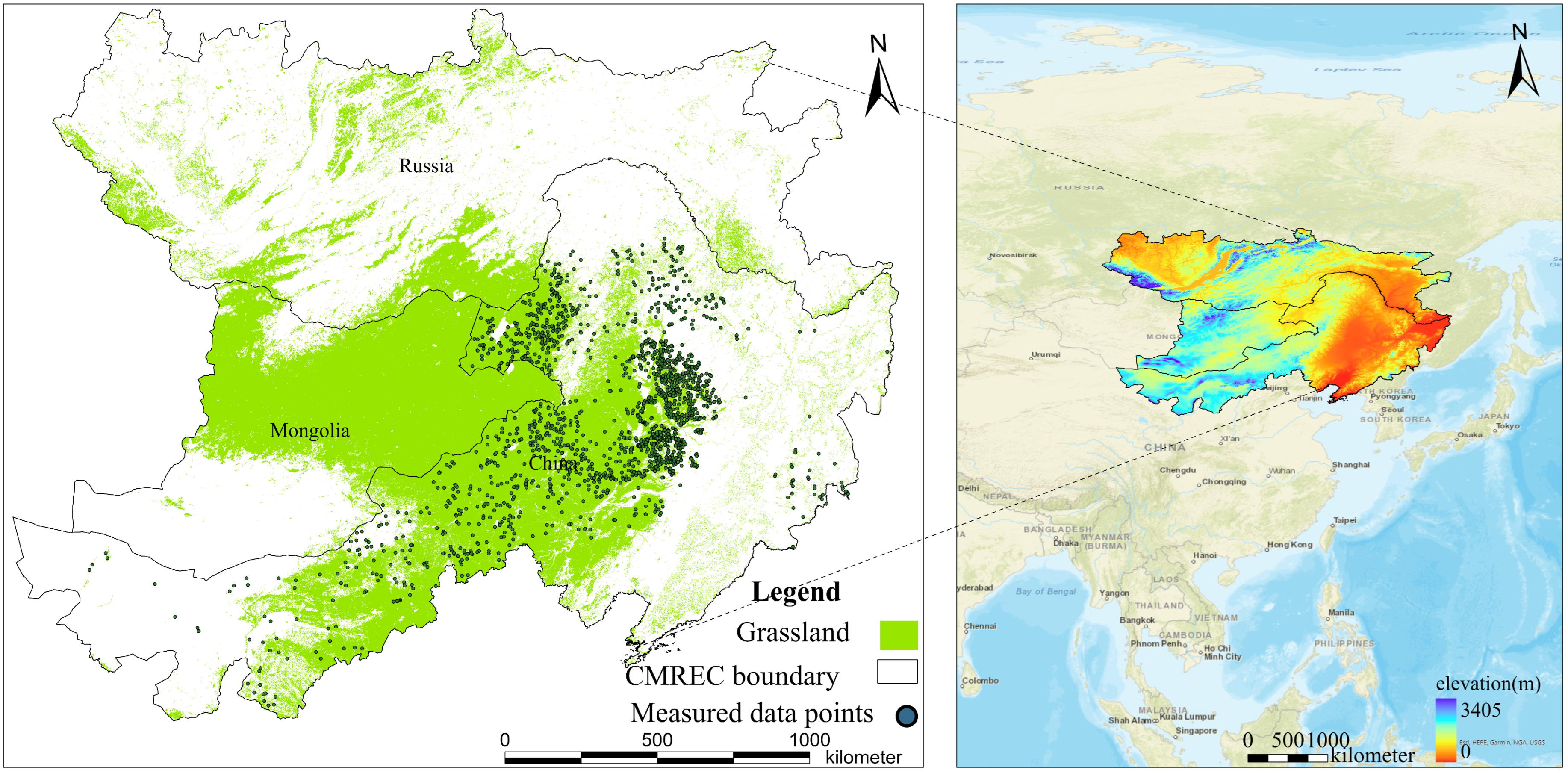
2.1. Study Area

The CMREC is situated in the northernmost region of the six economic corridors (37°24′–58°34′N and 97°7′–135°7′E) within the Belt and Road Initiative [42], which spans approximately 63.26 million km² and administratively encompasses four provinces in northern China, twelve provinces in eastern Mongolia, and five provinces in eastern Russia. The topographic structure of the study area is complex with elevation differences of more than 3000 m. In the east, the elevation gradually rises from the northeastern plains to the Mongolian Plateau, while in the west, it increases from the Central Siberian Plateau to the Yablonov Mountains. Climatic factors, including temperature and precipitation, vary significantly across the study area, ranging from arid to subpolar climates. The dominant climate is continental, characterized by long, cold, and dry winters, with rainfall concentrated during the warm summer months [43,44]. The landscapes of the three countries vary significantly due to differences in terrain, temperature, and precipitation. The main land cover types include grassland, cropland, barren land, and woodland [45]. Grasslands cover more than half of the landscape in Inner Mongolia, China and northwestern Mongolia, with the primary types being meadow grassland, typical grassland, and desert grassland. The grassland coverage in the study area is shown in Figure 1. Due to the influence of unique climatic and topographic conditions, the study area faces ecological and environmental challenges, such as soil erosion and dust storms. The northeast plain of China and Russia’s Far East region are marked by concentrated summer precipitation and significant freezing and thawing during winter and spring, which often leads to soil erosion and land degradation. The southern part of the Mongolian Plateau features expansive Gobi deserts, characterized by strong evaporation and frequent sand and dust storms. There are significant geographic disparities in economic development within the study area, with economic density generally higher in the south and lower in the north. Additionally, the economic totals of China and Russia are much higher than those of Mongolia. The Chinese northern plantation industry is relatively well-developed, while aquaculture plays a prominent role in Mongolia’s economy. In contrast, forestry production is the dominant sector in Russia.

2.2. Research Data

2.2.1. Time-Series Remote Sensing Data Products

The MOD13A3 dataset is a moderate-resolution imaging spectroradiometer (MODIS) product available on the Google Earth Engine (GEE) platform “https://earthengine.google.com/ (accessed on 11 April 2024)”, offering global vegetation indices, including NDVI and EVI, from February 2000 to the present. The spatial resolution of data is 1 km and the temporal resolution of is 1 month, offering monthly average values for NDVI and EVI. The RS data from April to October each year were used in this paper, spanning from 2000 to 2023. The MOD09A1 dataset, surface reflectance data from February 2000 to the present, was provided on the GEE platform. The surface reflectance dataset includes 7 bands, with a spatial resolution of 500 m and a temporal resolution of 8 days. The data of the red and near-infrared bands from April to October each year, from 2000 to 2023, were used to calculate the Soil-Adjusted Vegetation Index (SAVI). The monthly synthetic data is derived from the average SAVI values, where L is set to 0.5.

NDVI = (ρNir − ρRed)/(ρNir + ρRed)

(1)

EVI = 2.5 × (ρNir − ρRed)/(ρNir + 6 × ρRed − 7.5 × ρBlue + L)

(2)

SAVI = (1 + L) × (ρNir − ρRed)/(ρNir + ρRed + L)

(3)

2.2.2. Land Cover Data

MCD12Q1 is a global land cover classification dataset provided by the U.S. Geological Survey (USGS). The dataset is based on MODIS data, which includes land cover classification data globally from 2000 to 2022. The spatial resolution is 500 m, with 17 land cover classes, including forest, grassland, farmland, urban areas, and water bodies, etc. Among these, there are 16 land cover types of CMREC. In this paper, the data were resampled to a 1 km resolution and the grassland cover areas were extracted within the study area.

2.2.3. Topographic Data

Shuttle Radar Topography Mission (SRTM) Version 4 is a digital elevation model (DEM) dataset published by the National Aeronautics and Space Administration (NASA) in collaboration with the National Geospatial Intelligence Agency (NGA). The elevation data in this dataset could be used for applications such as terrain analysis, geological studies, and hydrological modeling. The resolution of this dataset is 1 arc second (about 30 m). In this paper, the data were resampled to a 1 km resolution to calculate topographic feature variables.

2.2.4. Meteorological Data

ERA5Land is a global land surface reanalysis meteorological dataset provided by the European Centre for Medium-Range Weather Forecasts (ECMWF). The spatial resolution of the dataset is approximately 9 km and the temporal resolution is 1 h, providing rich land surface meteorological data globally. In this study, the air pressure data from the ’ERA5-Land Monthly Aggregated-ECMWF Climate Reanalysis were downloaded on the GEE platform and resampled to a 1 km resolution for feature variable selection.

TerraClimate is a global climate dataset developed by the University of California, Irvine. The TerraClimate dataset consists of monthly data with a spatial resolution of approximately 4.6 km. The TerraClimate data used in this study were obtained from the GEE platform, including precipitation, maximum temperature, minimum temperature, and wind speed data for April to October each year from 2000 to 2023. The data were resampled to a 1 km resolution for feature variable selection.

2.2.5. The Field Measurement Data

The field investigation data in this study cover Heilongjiang Province, Jilin Province, Liaoning Province, and the Inner Mongolia Autonomous Region in China, ranging from 2019 to 2021, with focus on the summer months of July, August, and September. A sample plot was established within the sampling area with a resolution of 1 km. This plot contained 3 to 5 sample squares, with which the vegetation cover was measured. The average value of the vegetation cover from all sample squares within the plot was calculated to obtain the overall vegetation cover of the sample plot. Finally, data from 2362 sample points were collected.

2.3. Research Methodology

2.3.1. Machine Learning Regression

In constructing the GVC inversion model, in this paper, the RF regression model, XGBoost, and SVM regression were compared, and the model with the highest accuracy were adopted for inversion. In RF regression, multiple decision trees are constructed, with each tree trained on different randomly sampled datasets and feature sets. The robustness and generalization ability of the model were improved with the randomness of the sampled datasets, helping to avoid overfitting. GVC is primarily influenced by climatic and topographic conditions. Some researchers have included precipitation, elevation, slope, and aspect factors in their models [46]. As there are severe desertification and dust storm hazards in CMREC, the GVC in the region were also impacted significantly by factors such as wind speed and air pressure. Therefore, for the constructed inversion model, 16 feature variables were selected in this study, including vegetation index variables, spectral variables, geographic variables, and meteorological variables, as shown in

Table 1. Characterization variables for inversion of GVC.

Type of Data	Secondary Data Type	Spatial Resolution	Years	Data Sources
Vegetation Index Data	NDVI	1 km	2000–2023 April–October	MOD13A3
	EVI
	SAVI	500 m → 1 km		MOD09A1
Topography Data	DEM	30 m → 1 km	/	SRTM Version 4
Meteorological Data	Tmmx	4.6 km → 1 km	2000–2023 April–October	TerraClimate
	Tmmn
	Precipitation
	Wind speed
	Soil moisture
	Air pressure	11.1 km → 1 km		ERA5Land

.

R² and root mean square error (RMSE) were selected for the training set, while RMSE, the correlation coefficient r between predicted and measured values, and cross-validation root mean square error (CVRMSE) were selected for the test set to evaluate model accuracy. CVRMSE indicates the model’s fitting effect. The smaller the value is, the better the model fit. A CVRMSE of 0–10% is excellent, 10–20% is good, and 20–30% is fair.

$${\mathrm{R}}^2={\displaystyle \frac{{\sum }_{\mathrm{i}=1}^{\mathrm{n}}({\mathrm{y}}_{\mathrm{i}}-{\widehat{\mathrm{y}}}_{\mathrm{i}}{)}^2}{{\sum }_{\mathrm{i}=1}^{\mathrm{n}}({\mathrm{y}}_{\mathrm{i}}-{\overline{\mathrm{y}}}_{\mathrm{i}}{)}^2}}$$

(4)

$$\mathrm{RMSE}=\sqrt{{{\sum }_{\mathrm{i}=1}^{\mathrm{n}}({\mathrm{y}}_{\mathrm{i}}-{\widehat{\mathrm{y}}}_{\mathrm{i}})}^2/\mathrm{n}},$$

(5)

$$\mathrm{CVRMSE}={\displaystyle \frac{\mathrm{RMSE}}{\overline{\mathrm{y}}}\times 100\%,}$$

(6)

$$\mathrm{r}={\displaystyle \frac{\mathrm{n}(\sum \mathrm{xy})-(\sum \mathrm{x}\left)\right(\sum \mathrm{y})}{\sqrt{[\mathrm{n}\sum {\mathrm{x}}^2-\left(\sum \mathrm{x}{)}^2\left]\right[\mathrm{n}\sum {\mathrm{y}}^2-(\sum \mathrm{y}{)}^2\right]}}}$$

(7)

where, n represents the number of test samples, ${\widehat{\mathrm{y}}}_{\mathrm{i}}$ and y_i are the predicted and measured values of GVC of the test samples, respectively, indicating the average value of the test samples. x is the measured value of GVC. y is the predicted value of GVC.

In constructing the RF regression model, in this paper, 2362 data points were divided into training and test sets with a 7:3 ratio. Then, the features are ranked by importance and the least important ones are removed. The accuracy is re-evaluated after each removal, and the process continues until the model achieves the highest accuracy, leading to the optimal set of feature variables. In this study, 10 feature variables were selected, including NDVI, EVI, SAVI, DEM, maximum temperature (Tmmx), minimum temperature (Tmmn), precipitation, soil moisture, wind speed, and air pressure.

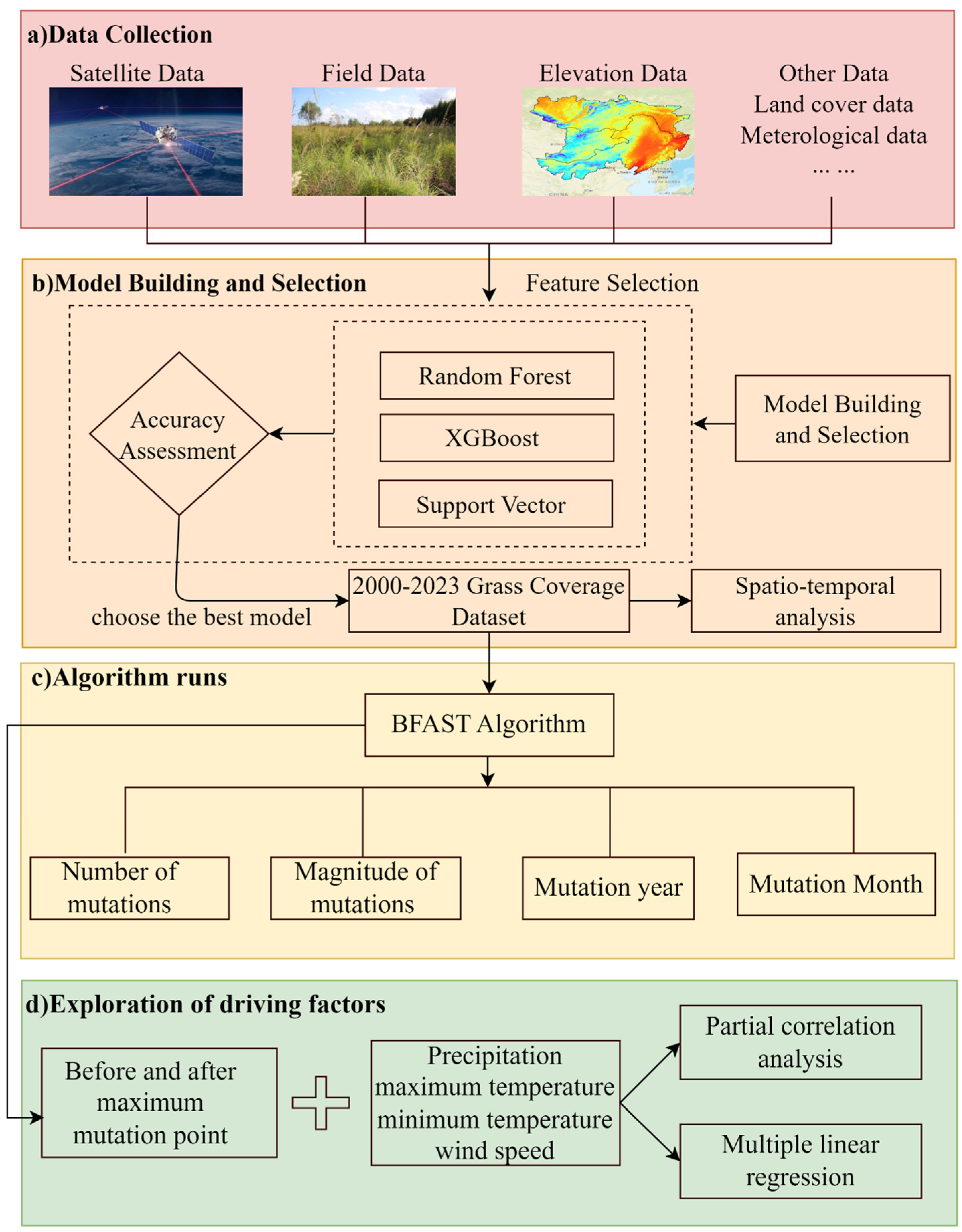
2.3.2. Technology Roadmap

Figure 2 is the technical roadmap of this study.

First, the feature selection process is introduced. The RS satellite data were used, and the field measured data and elevation data were selected as the original dataset for feature selection. The feature variables were ranked by their importance.

In the second part, model building and selection were focused on. The model’s fitting accuracy is evaluated using performance metrics, and the RF regression model with the highest accuracy is chosen to estimate GVC, producing the CMREC time series dataset for GVC from April to October 2000 to 2023.

The third part involves mutation monitoring, where the BFAST algorithm is applied to extract information on the number, magnitude, year, and month of mutations, providing data support for subsequent driver analysis.

Finally, partial correlation analysis and multiple linear regression were conducted on the driving factors before and after the maximum mutation point to analyze their influence on GVC and the degree of this influence, providing support for regional grassland ecological protection.

2.3.3. BFAST Mutation Detection

The BFAST algorithm, proposed by J. Verbesselt et al. in 2010 [33], which decomposes the original time series into seasonal, trend, and residual components using iterative time series, is effective at detecting seasonal and trend changes in RS imagery time series in semi-arid regions. The BFAST algorithm is an additive decomposition model using segmented linear trend fitting and a seasonal trend model, with a wide range of applications in meteorology, hydrology, and economics. The BFAST formula for long time-series is as follows:

Y_t′ = T_t′ + S_t′ + e_t′ (t′ = 1, 2, …, n)

(8)

where Y_t′ represents the observed data, T_t′ is the trend component, S_t′ is the seasonal component, e_t′ is the residual component, and t′ is the observation time.

The trend component T_t′ is fitted to each segment using a linear model, where for each segment t^′*_i < t^′ ≤ t′^*_i+1, with t′₀ defined as 0. The linear model fitted is:

T_t′ = α_i + β_it′,

(9)

where i = 1, …, m, with m being the total number of mutations; α_i and β_i represent the intercept and slope of the linear model, respectively.

The seasonal component S_t′ is fitted using a segmented linear model for each segment, where t′^*_j < t′ ≤ t′^*_j+1, with t′₀ defined as 0. The linear model fitted is:

$${\mathrm{s}}_{\mathrm{t}\prime }=\sum _{\mathrm{k}=1}^{\mathrm{j}}{\mathsf{\delta }}_{\mathrm{j},\mathrm{k}}\sin ({\displaystyle \frac{2\mathsf{\pi }\mathrm{k}\mathrm{t}\prime }{\mathrm{f}}}+{\mathsf{\delta }}_{\mathrm{j},\mathrm{k}})$$

(10)

where j represents the location of mutations, taking values from 1 to q, with q being the total number of mutations; k denotes the number of reconciliation terms; ${\mathsf{\delta }}_{\mathrm{j},\mathrm{k}}$ is the amplitude; ${\mathsf{\delta }}_{\mathrm{j},\mathrm{k}}$ is the phase; f is the frequency.

This paper focuses on the mutations of GVC from April to October in the CMREC dataset from 2000 to 2023. The information about mutations includes their number, timing, and magnitude. Among them, the mutation timing includes both the year and month scales of the mutations. The BFAST algorithm in this paper is implemented by the BFAST package for the R language “https://cran.r-project.org/web/packages/bfast/index.html (accessed on 23 May 2024)”.

2.3.4. Partial Correlation Analysis

Partial correlation analysis is a statistical method used to measure the correlation between two variables, characterized by calculating the net correlation between variables after controlling for the effects of other variables. In environmental and ecological studies, vegetation changes are often influenced by a combination of factors, such as climatic conditions, soil properties, and human activities. Therefore, simple correlation analysis may be disturbed by confounding variables and cannot accurately reveal the independent contribution of climatic factors to vegetation change.

In this paper, precipitation (prec), average temperature (tmean), and wind speed (vs) were selected for bias correlation analysis. Where the maximum and minimum temperatures are averaged to obtain the average temperature. The higher-order partial correlation coefficients are calculated as follows:

$${\mathrm{R}}_{\mathrm{ij},{\mathrm{l}}_1.{\mathrm{l}}_2\dots {\mathrm{l}}_{\mathrm{g}}}={\displaystyle \frac{{\mathrm{R}}_{\mathrm{ij},{\mathrm{l}}_1.{\mathrm{l}}_2\dots {\mathrm{l}}_{\mathrm{g}-1}}-{\mathrm{R}}_{\mathrm{i}{\mathrm{l}}_{\mathrm{g}},{\mathrm{l}}_1.{\mathrm{l}}_2\dots {\mathrm{l}}_{\mathrm{g}-1}}{\mathrm{R}}_{\mathrm{j}{\mathrm{l}}_{\mathrm{g}},{\mathrm{l}}_1.{\mathrm{l}}_2\dots {\mathrm{l}}_{\mathrm{g}-1}}}{\sqrt{(1-{{\mathrm{R}}^2}_{\mathrm{i}{\mathrm{l}}_{\mathrm{g}},{\mathrm{l}}_1.{\mathrm{l}}_2\dots {\mathrm{l}}_{\mathrm{g}-1}}\left)\right(1-{{\mathrm{R}}^2}_{\mathrm{j}{\mathrm{l}}_{\mathrm{g}},{\mathrm{l}}_1.{\mathrm{l}}_2\dots {\mathrm{l}}_{\mathrm{g}-1}})}}}$$

(11)

where ${\mathrm{R}}_{\mathrm{ij},{\mathrm{l}}_1.{\mathrm{l}}_2\dots {\mathrm{l}}_{\mathrm{g}}}$ is the g-th order partial correlation coefficient, and the right-hand side of the equation represents the (g − 1)-th order partial correlation coefficient.

In this paper, the variables such as prec (P), tmean (T), vs (V), and GVC (G) were considered, where k = 4. For example, for two variables, GVC and prec, the sample partial correlation coefficient of order g = 2 (where g ≤ k − 2) is calculated as follows:

$${\mathrm{R}}_{\mathrm{G}\mathrm{P},\mathrm{T}\mathrm{V}}={\displaystyle \frac{{\mathrm{R}}_{\mathrm{G}\mathrm{P}}-{\mathrm{R}}_{\mathrm{G}\mathrm{V},T}{\mathrm{R}}_{\mathrm{PV},T}}{\sqrt{(1-{{\mathrm{R}}^2}_{\mathrm{G}\mathrm{P},T}\left)\right(1-{{\mathrm{R}}^2}_{\mathrm{PV},T})}}}$$

(12)

2.3.5. Multiple Linear Regression

Additionally, to quantify the overall impact of climate change on vegetation changes, in this paper, a multiple linear regression model was developed to identify the drivers of change affecting CMREC grasslands, where the maximum and minimum temperatures are averaged to obtain the average temperature. The equations for the regression model and predictor variables are shown below:

Grassland Coverage = a * prec + b * tmean + c * vs

(13)

where a, b, c, are the multiple linear regression coefficients.

In multiple linear regression analysis, there may be a high degree of correlation between independent variables, which can lead to inaccurate estimation of regression coefficients and reduce the explanatory power of the model. In order to ensure the reliability of the model, this paper uses Variance Inflation Factor (VIF) to test the multicollinearity between independent variables, and the formula of VIF is as follows:

$${\mathrm{VIF}}_{\mathrm{i}}={\displaystyle \frac{1}{1-{\mathrm{R}}_{\mathrm{i}}^2}}$$

where ${\mathrm{R}}_{\mathrm{i}}^2$ is the coefficient of determination obtained by regressing the ith independent variable on the other independent variables.

The larger the VIF value is, the stronger the covariance is between the independent variables. Usually, a VIF value of less than 5 indicates a weak covariance, which is acceptable; a VIF value of more than 10 indicates the existence of serious multiple covariance, which needs further treatment. In this paper, the VIF values of each climate factor are calculated, and the results show that the VIF values of the independent variables are all less than 5, indicating that there is no serious multicollinearity problem between the independent variables in the model, and the results of the regression model are reliable.

3. Results

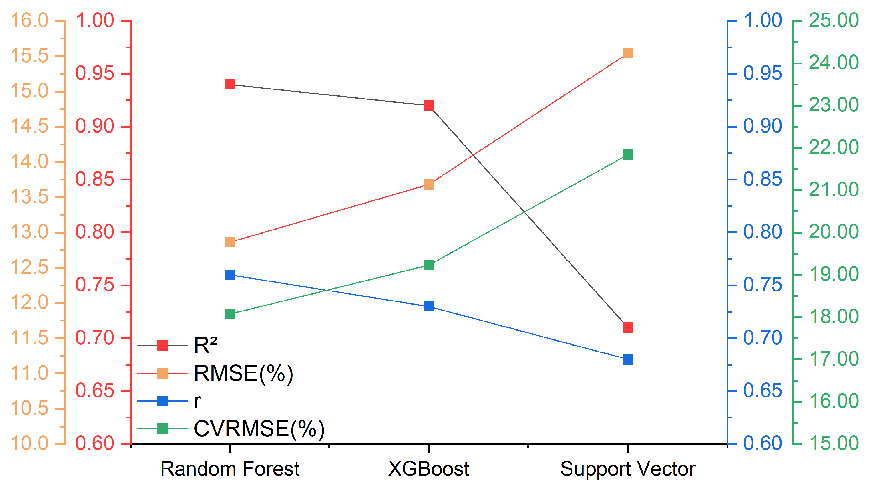
3.1. Evaluation of the Accuracy of the Regression Model

The accuracies of different models are presented in Figure 3. RF achieves the highest accuracy, with an R² of 0.94 for the training set, an RMSE of 12.86% for the test set, a correlation coefficient of 0.76 between predicted and actual values, and a CVRMSE of 18.07%. This is followed by XGBoost with a training set R² of 0.92, a test set RMSE of 13.68%, a correlation coefficient of 0.73 between predicted and actual values, and a CVRMSE of 19.23%. The model with the lowest accuracy was SVM Regression, where R² was 0.71 for the training set, RMSE was 15.54% for the test set, the correlation coefficient was 0.68 between predicted and actual values, and CVRMSE was 21.84%. Each accuracy metric of RF outperformed the other two models, so the RF regression model was selected for inverting GVC from April to October during the period 2000–2023 in CMREC. Compared to RF and XGBoost, SVM may be limited by the ability to express complex nonlinear relationships during the training process, as well as being more sensitive to data size and outliers, resulting in the lowest prediction accuracy.

3.2. Spatial Distribution of Grassland Vegetation Cover

Based on the characteristic variables of April–October during the grassland growing season from 2000 to 2023, the monthly GVC of each image element was estimated using RF regression. As shown in Figure 4, using the inversion results of GVC for 2022 as an example, the spatial distribution reveals relatively low GVC in Inner Mongolia, China and parts of Mongolia in the southwest, due to extensive wasteland and serious desertification. In contrast, the northeastern regions are dominated by forests and grasslands, resulting in higher grassland coverage. Regarding temporal distribution, the overall GVC exhibited an increasing and then decreasing trend from April to October, following the growth patterns of grassland vegetation, with a peak in July–August.

3.3. BFAST Mutation Information Extraction

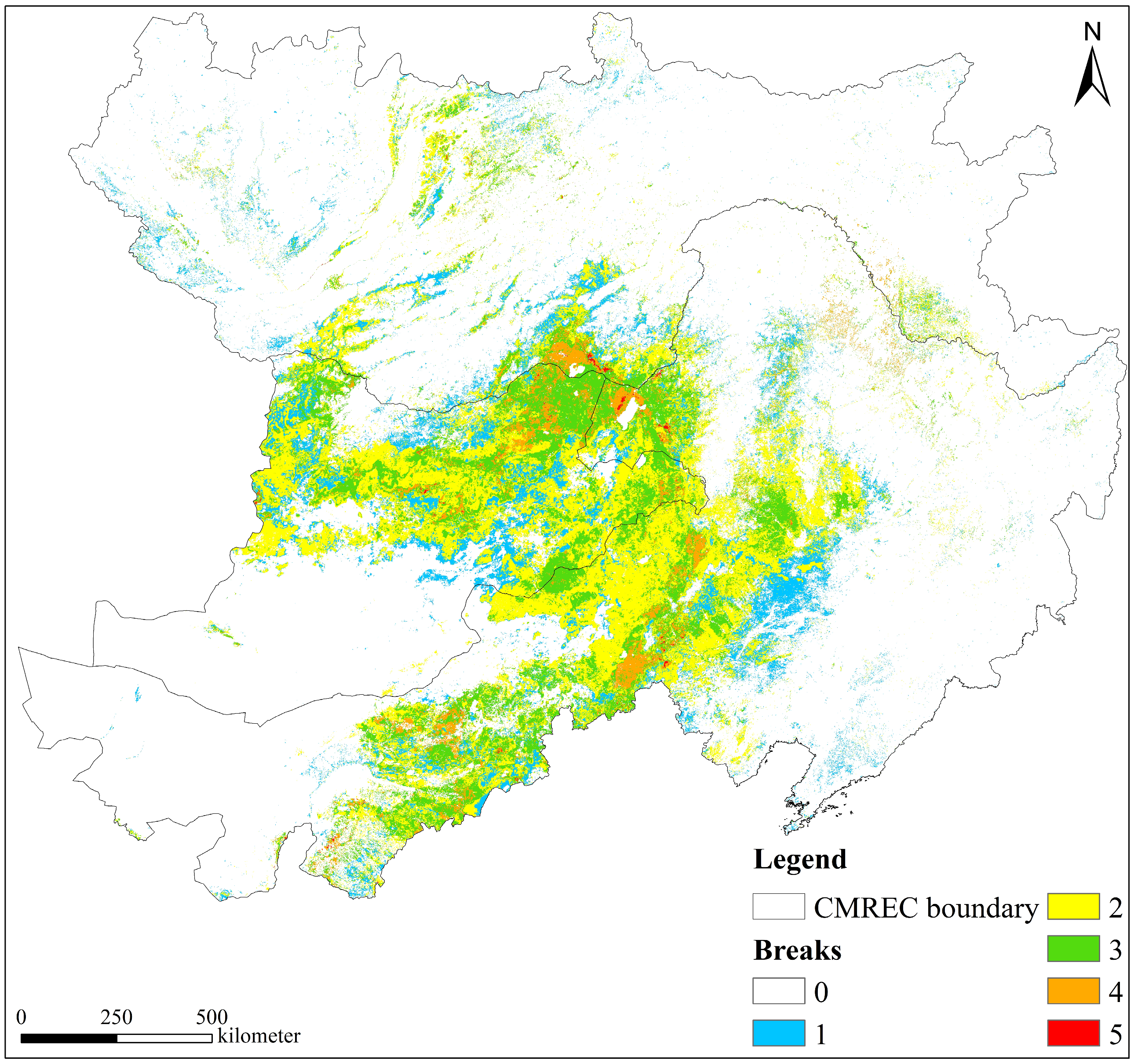
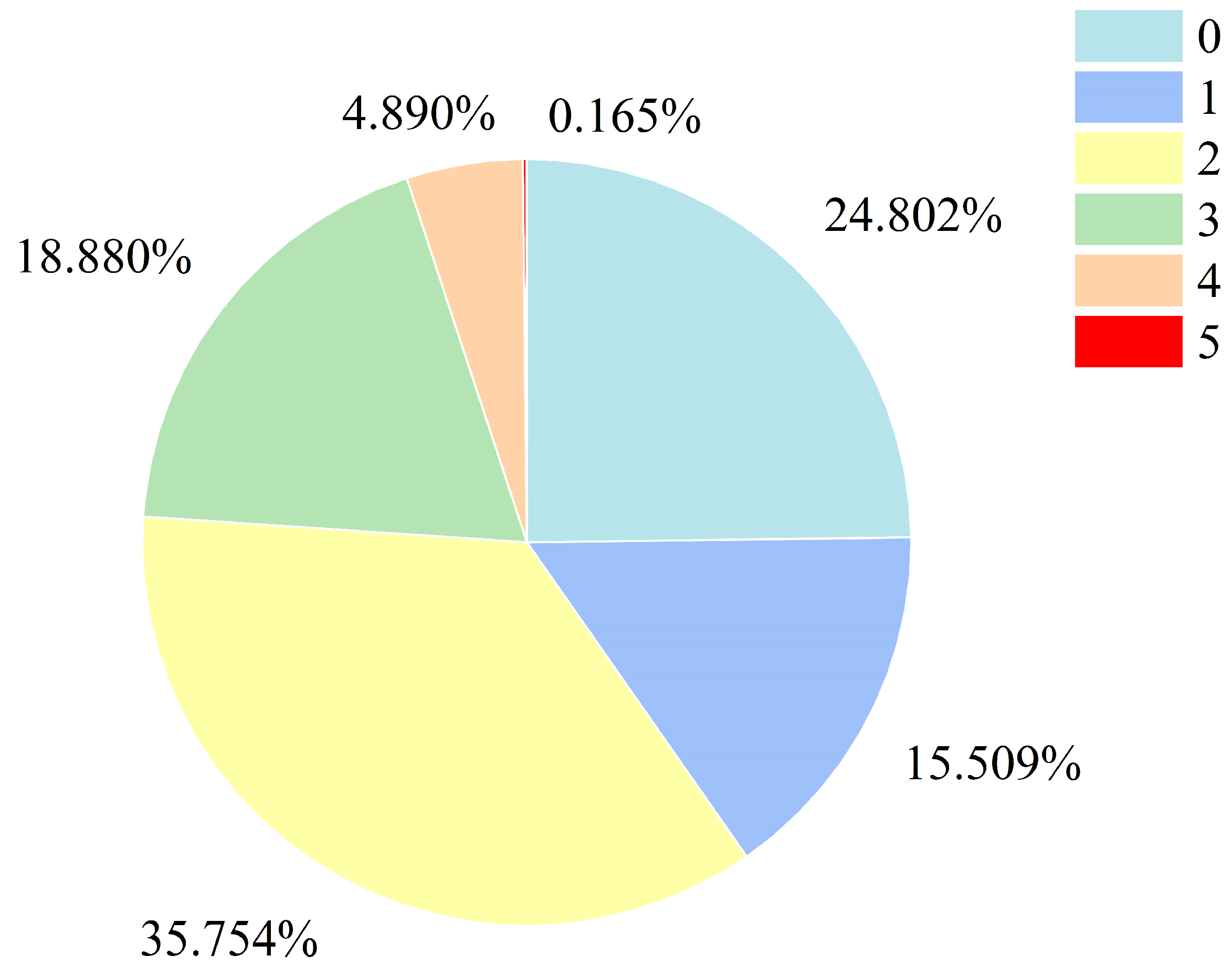
3.3.1. Number of Mutations

As shown in Figure 5 and Figure 6, the number of GVC mutations from April to October between 2000 and 2023 in CMREC and their proportions are presented. The figures reveal that mutations are mainly concentrated in the Inner Mongolia region of China, parts of Mongolia, and the tri-border area between China, Mongolia, and Russia, with most mutations occurring 1–2 times. Mutations occurring more than 3 times account for a relatively small proportion, primarily located in Inner Mongolia, China and the tri-border region.

The grasslands in the study area were influenced by various factors, with the number of mutations in vegetation coverage ranging from 0 to 5. Then, 75.198% of the grasslands experienced at least one mutation. The highest proportion was for 2 mutations, 35.754%, followed by 3 mutations, 18.880%, and 1 mutation, 15.509%. The least number of mutations were 4 and 5 mutations, which accounted for only 4.890% and 0.165% of all mutations.

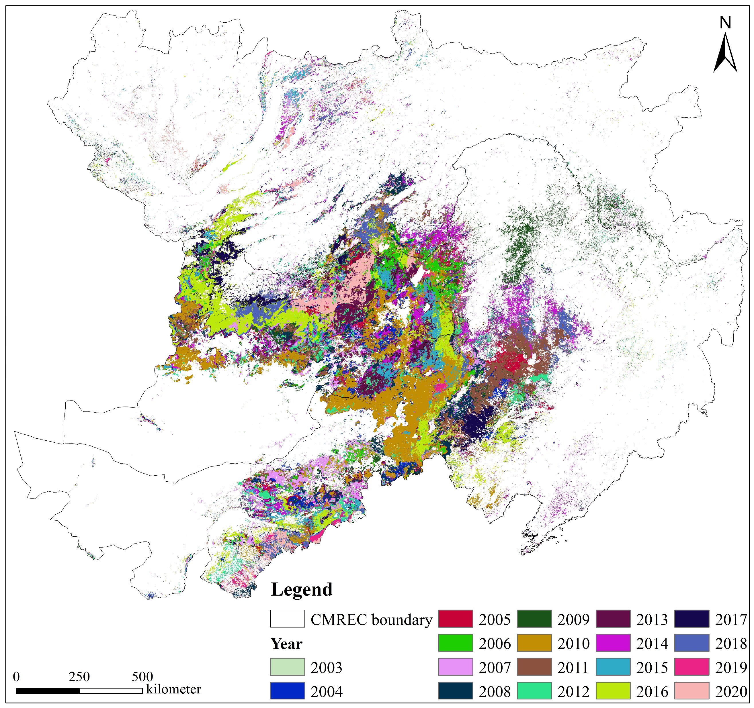
3.3.2. Year of Maximum Mutations

Figure 7 shows the years with the maximum mutations for the April–October grassland in CMREC from 2000 to 2023. As shown in the figure, mutations occurred nearly every year within the study period. In 2010 and 2017, large areas of grassland mutations occurred in the Inner Mongolia region of China, followed by 2016 and 2020, when contiguous grassland mutations were also observed in parts of Mongolia.

The percentage of years in which maximum mutations occurred is shown in Figure 8. The fewest mutations occurred in 2003 and followed by 2019, with no significant mutations observed, accounting for only 1.189% and 1.769% of all years, respectively. The years with the highest percentage of mutations were 2010 followed by 2016, accounting for 14.573% and 11.604% of all mutations, respectively, and marking the only two years when the percentage of mutations reached 10% or more. The remaining mutation years were more balanced, mostly between 2% and 7%.

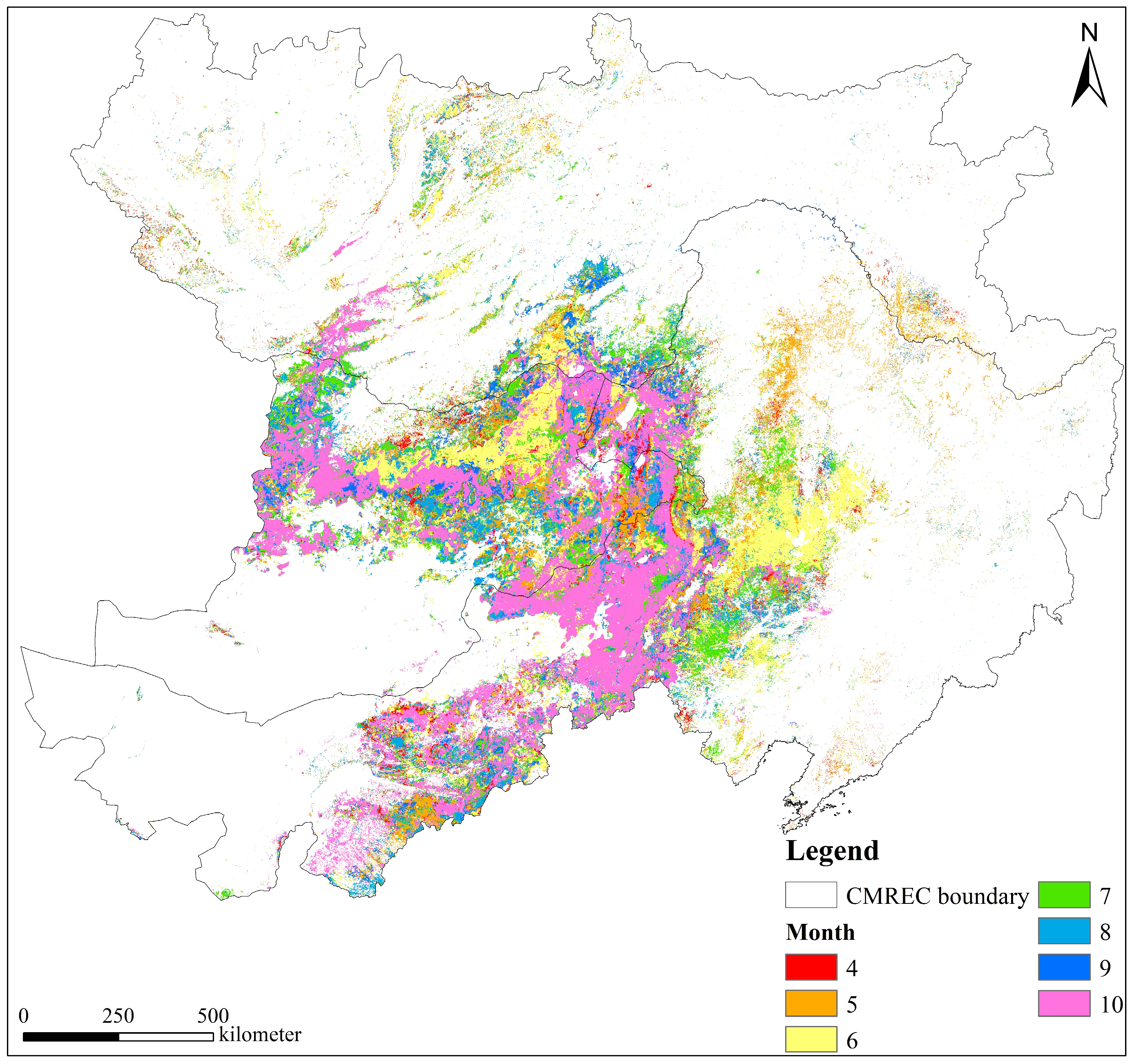
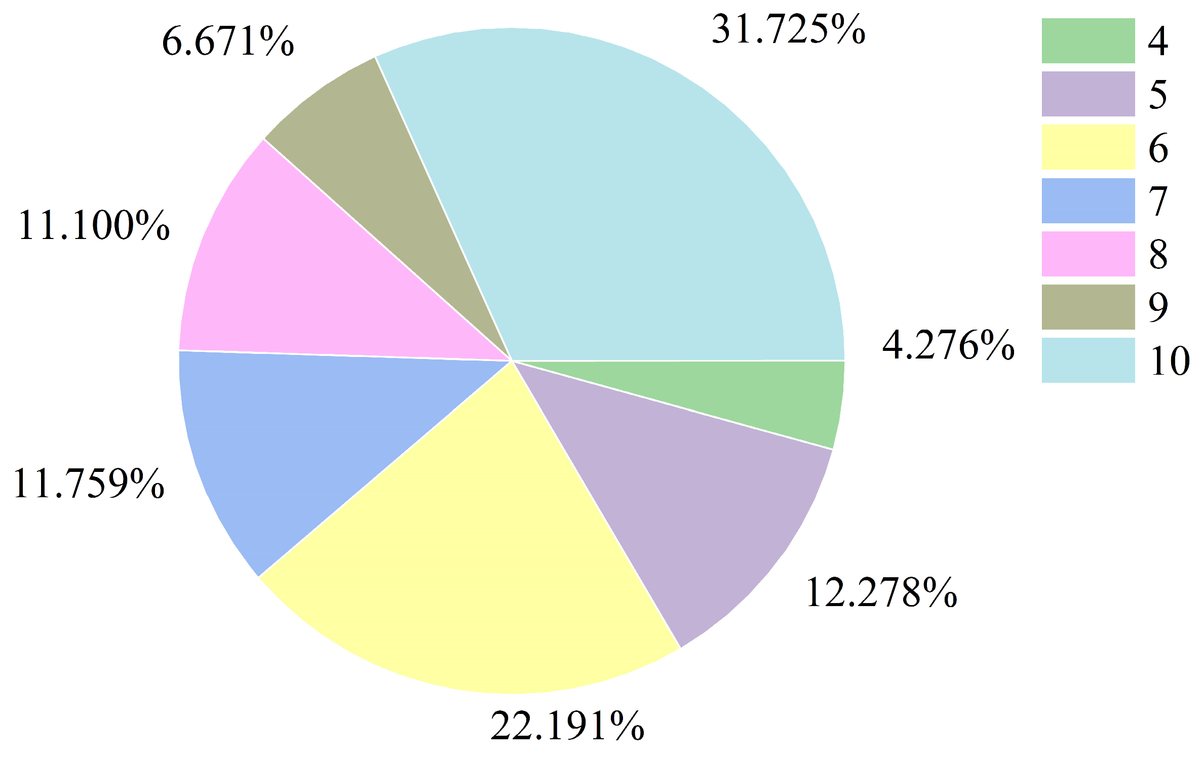
3.3.3. Month of Maximum Mutations

As shown in Figure 9, the months with the maximum mutations in GVC occurred from April to October. Mutations in June and October mainly occurred in Inner Mongolia, China and parts of Mongolia. There were few grassland mutations in Russia, and no specific month showed maximum mutations.

Figure 10 shows the percentage of months with maximum mutations. The greatest number of mutations occurred in October followed by June, accounting for 31.725% and 22.191% of all mutations, respectively. They were followed by May, July, and August, each contributing about 11% to 12% of the total grassland mutations. April was the lowest percentage of mutations, accounting for only 4.276% of all monthly mutations.

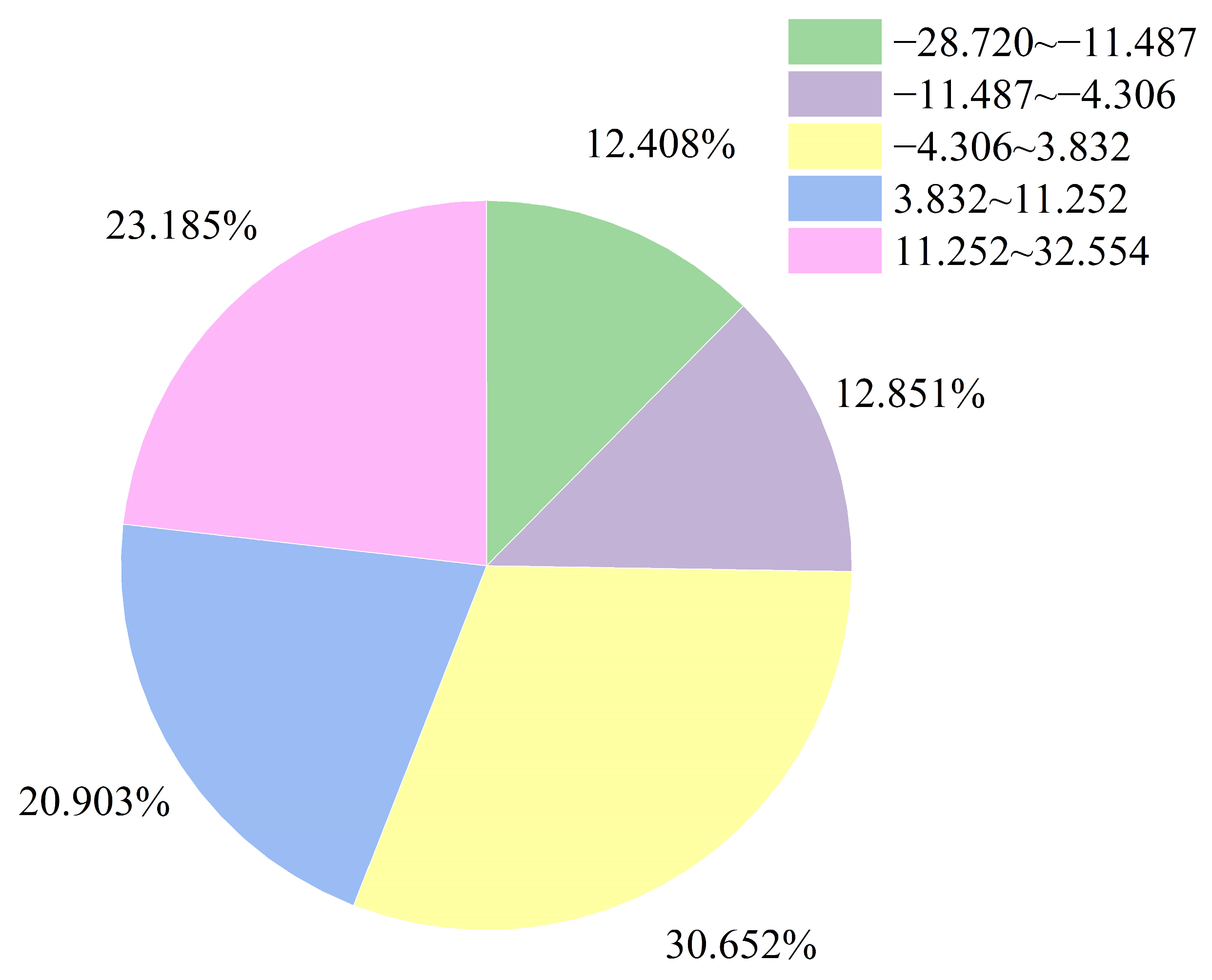
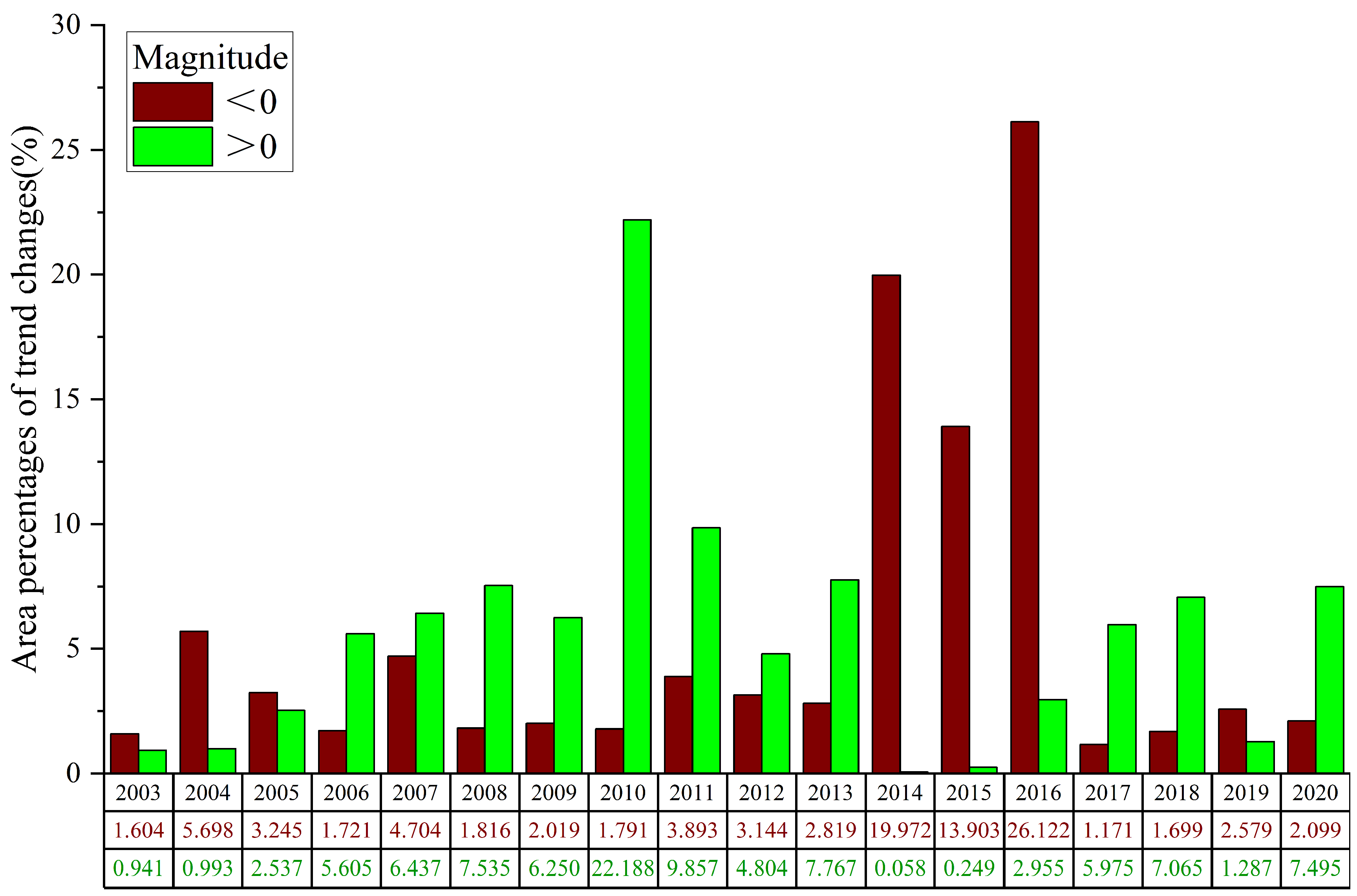
3.3.4. Magnitude of Mutations

Figure 11 shows the magnitude of mutations in GVC. Negative mutations reflected a reduction in vegetation coverage due to external factors, primarily concentrated in Inner Mongolia, China and parts of Mongolia. Positive mutations indicated an increase in vegetation coverage, mainly concentrated in parts of Inner Mongolia, China and the border area of the three countries.

In this paper, the magnitude of mutations is categorized into five ranges by the natural breakpoint method, such as a large decrease, a slight decrease, essentially unchanged, a slight increase, and a large increase. The magnitude of mutations is shown in Figure 12. The magnitude of mutations in grassland was −4.306 to 3.832, accounting for 30.652% of the total; 23.185% of the grassland had positive mutations of at least 11%, indicating that the grassland was elevated by external influences. The mutations with a decrease of 11.487% and above accounted for the smallest proportion at 12.408% of all mutations, indicating that the proportion of mutations with a large decrease in the study area was relatively small.

As shown in

Table 2. Percentage of mutation magnitude at each breakpoint.

Breakpoints	−28.720~−11.487	−11.487~−4.306	−4.306~3.832	3.832~11.252	11.252~32.554
1	7.108%	13.151%	29.279%	46.051%	4.411%
2	18.524%	23.165%	3.093%	28.200%	27.018%
3	18.763%	11.940%	1.036%	17.427%	50.834%
4	22.383%	5.531%	0.158%	7.712%	64.215%
5	27.765%	2.866%	0.029%	6.630%	62.710%

, the percentage of mutation magnitudes for each breakpoint was presented. For regions with fewer mutations, such as those with only 1 mutation, the magnitude of mutations was minimal, being primarily distributed in the 3.832~11.252 interval, followed by the −4.306~3.832 and −11.487~−4.306 intervals. This suggests that regions with fewer mutations exhibit only slight changes in vegetation. Two mutations are primarily concentrated in the 3.832~11.252 interval. As the number of mutations increases, a higher proportion of mutations fall within the 11.252~32.554 interval, indicating that grasslands in regions with more mutations are developing in a more positive direction.

Figure 13 shows the brown and green mutations in the grassland across different years. Brown mutations in grasslands typically indicate ecosystem stress or degradation, while green mutations reflect a healthy and stable ecological state. The grassland exhibited the highest green mutations in 2010 and the highest brown mutations in 2016. Significant differences were observed between brown and green mutations in the grassland during each year of the study period. The brown mutations in GVC were greater than the green mutations until 2005, while the overall green mutations exceeded the brown mutations from 2017 to 2019, showing a positive trend. In 2019, brown mutations were greater than green mutations, whereas in 2020, green mutations surpassed brown mutations. Hence, the grassland shifted from brown to green mutations between 2019 and 2020, suggesting that GVC has been improving in recent years.

Figure 14 shows the brown and green mutations in GVC across different months. The grassland exhibited the highest green and brown mutations in October. Throughout the study period, there were differences between brown and green mutations in grasslands, with brown mutations exceeding green mutations during all July–August months. Initially, brown mutations were greater than green mutations in July, while green mutations surpassed brown mutations in October. The results indicate that GVC was shifting toward green mutations, with an overall trend towards improvement during the grass growing season.

3.4. Driving Factor Analysis

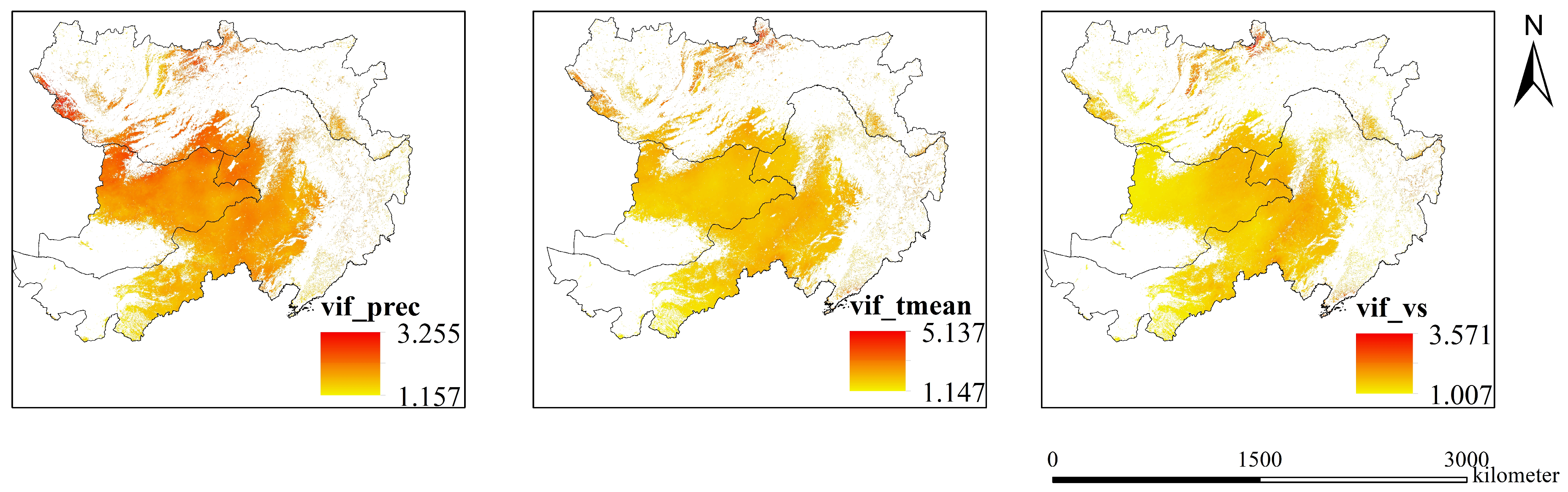
3.4.1. Multicollinearity Test

The spatial distribution of the VIF values of the three driving factors is demonstrated as shown in Figure 15. The VIF values of precipitation and wind speed are significantly lower than 5, indicating that there is no significant multicollinearity problem in the model for these two variables. Although a small number of VIF values of mean temperature exceeded 5 in the fringe zone of the study area, their proportion was low and their spatial distribution was more limited, which did not significantly affect the stability of the model as a whole. Therefore, the multiple linear regression model in this study has high reliability and is suitable for exploring the coefficient changes of each climate factor before and after the maximum mutations.

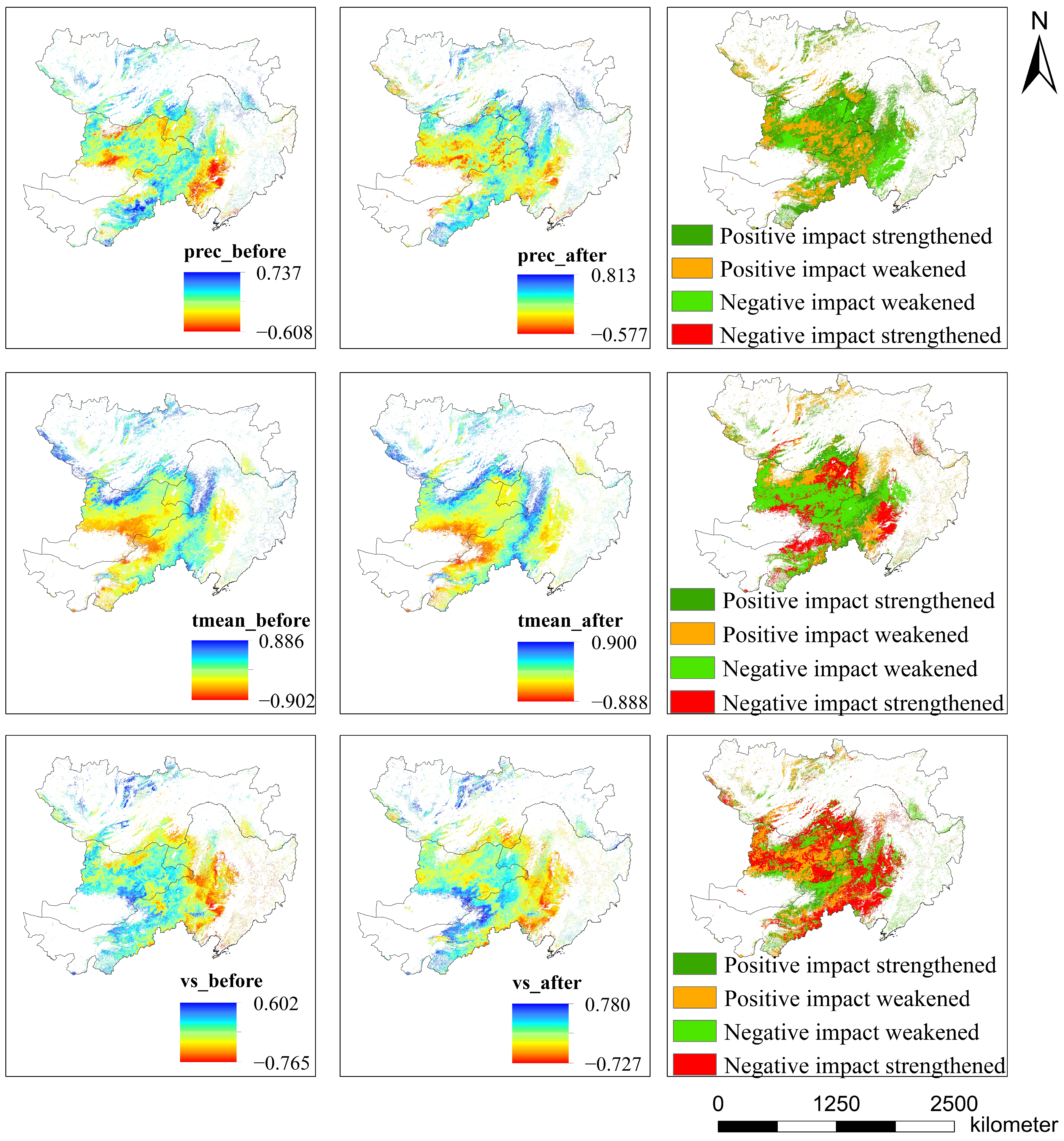
3.4.2. Partial Correlation Analysis Results Analysis

As shown in Figure 16, the results of the bias correlation analysis coefficients of the three driving factors, including precipitation, mean temperature, and wind speed, as well as their positive and negative impacts before and after the maximum mutations are demonstrated. Specifically, the negative impact of mean temperature on grassland was enhanced in the central and southern parts of the study area, especially in parts of Mongolia, parts of Inner Mongolia in China, and the tri-border area, where the enhancement of the negative impact accounted for 23% of all the changes, and the rest of the changes accounted for a small difference in the percentage. In these regions, GVC decreased significantly with increasing mean temperature and the magnitude of the decrease increased. As for precipitation, there was a 49% enhancement of positive effects as well as only 1% enhancement of negative effects, indicating that the bias correlation coefficients of precipitation were enhanced after maximum mutations in nearly half of the regions, which is a positive effect on GVC. The opposite of precipitation was wind speed, which had a 42% negative effect enhancement after the maximum mutations occurred, indicating that wind speed had a mainly negative effect on GVC. Among the three drivers, it was precipitation, followed by mean temperature, and finally wind speed, that had more positive effects after mutations. The most enhanced negative effect was wind speed, followed by mean temperature, whereas precipitation had the least negative effect.

3.4.3. Multiple Linear Regression Results Analysis

As shown in Figure 17, the results of the multiple linear regression coefficients of the various driving factors and their positive and negative impacts before and after the maximum mutations are demonstrated. As with the partial correlation analysis, the multiple linear regression coefficients of the three driving factors showed different degrees of expansion after the maximum mutation occurred, which indicated that both positive and negative impacts of the maximum mutations caused the overall impact to be further strengthened. Specifically, the negative effect of mean temperature on grasslands was enhanced in the southern part of the study area, especially in parts of Inner Mongolia, China. In these regions, GVC decreased significantly with increasing mean temperature, and the magnitude of this decrease increased. Precipitation had 43% of its positive impacts enhanced and 36% of its positive impacts weakened before and after the maximum mutations, with only 1% of negative impacts enhanced. The multiple linear regression coefficients of precipitation before and after the maximum mutations did not change much, suggesting that the impacts of precipitation on grasslands were relatively robust and basically focused only on positive impacts. The opposite of precipitation was wind speed, which had a 45% increase in negative effect after the maximum mutation occurred, indicating that wind speed had an enhanced negative effect on nearly half of the grasslands after the mutations. This effect was most pronounced in the Inner Mongolia region of China, the Mongolian steppe, and the border between China, Mongolia, and Russia. Among the three driving factors, wind speed was the most affected by mutations, followed by mean temperature and precipitation, suggesting that the effect of precipitation on GVC was relatively stable, which might be related to water management or vegetation adaptation in the region.

3.4.4. Policy Implications

In this study, the driving effects of precipitation, mean temperature, and wind speed on GVC were investigated through partial correlation analysis and multiple linear regression before and after the maximum mutation. The results showed that the positive effect of precipitation on GVC was relatively stable before and after mutations. However, the effect of wind speed varied significantly, and the negative effect of wind speed on vegetation cover increased in nearly half of the area. This phenomenon is particularly prominent in the Inner Mongolia region of China, Mongolia, and the tri-border area between China, Mongolia, and Russia.

Grassland ecosystems in these regions are fragile and are highly affected by wind erosion, sanding, and desertification. In response to the increasing negative impacts of wind speed, policymakers should prioritize the implementation of wind and sand control measures, such as vegetation restoration, grassland fence protection, and windbreak construction. At the same time, grassland degradation monitoring can be strengthened, grassland management policies can be optimized, and cross-border cooperation can be promoted to jointly address grassland ecological degradation. Such comprehensive and regional policy measures will help to improve the stability and resilience of grassland ecosystems.

4. Discussion

Using the GEE cloud platform and R language, multi-source RS datasets from the study area were easily collected and integrated with vegetation, soil, topography, and climate data to monitor the long-term dynamics of GVC over large-scale regions [47,48]. When GVC in CMREC were extracted, the RF model outperformed XGBoost and SVM methods which could be used to detect changes in GVC within the CMREC region. The spatial and temporal changes in GVC within CMREC follow the general pattern of the growing season, which increases from April to July, peaks in July and August, and then decreases until October [49]. However, the accuracy of identifying changes in GVC patterns may be impacted by the current downscaling of vegetation, soil, topography, and climate metrics at varying resolutions within the CMREC region [50]. Additionally, a deep learning approach for extracting GVC could further help distinguish differences between land cover types [51,52].

In this paper, the insights were offered into the spatial and temporal variations in GVC and the causes of mutations in CMREC. Temporally, mutations occurred throughout most of the study period. Spatially, nearly 60% of the area similarly experienced at least 1 mutation. The application of the BFAST method to CMREC areas with high GVC supports the work of Verbesselt et al., who demonstrated the suitability of BFAST for global-scale disturbance monitoring [35]. Meanwhile, the overlay analysis of mutation information from various aspects, such as the magnitude of mutations in different numbers of mutations, could assist local governments in targeting effective protection and management of grassland ecological resources. In this paper, the accurate timing of mutations down to the month was also provided, offering the possibility of studying mutation occurrence on a finer temporal scale in the future. In addition, the mutation data showed that brown mutations outnumbered green mutations in July and August, which deviates from the peak grass growth period predicted by seasonal climate models. Under the influence of climatic factors, summer is typically the most vigorous period for grass growth, particularly when the moisture and temperature conditions are favorable. Thus, the increase in brown mutations may indicate anomalies in grass growth conditions. However, this phenomenon may also result from anthropogenic disturbances such as land-use changes, agricultural activities, or other human activities, particularly during these months of high grass growth, which may involve increased grassland management or utilization activities such as grazing and farming [53,54].

In this paper, since the anthropogenic data such as population and GDP data are only on an annual scale, BFAST is unable to detect temporal seasonal variations in them. These potential factors cannot be considered during the driving analysis. As a result, the mutation analysis focuses only on the impact of climatic factors, without further consideration of anthropogenic influences. To explore the potential influence of anthropogenic factors on grassland mutations more comprehensively, future studies could incorporate more detailed time-series data. For instance, monthly or quarterly data on factors such as population density, land use changes, and agricultural activity frequency could help clarify the role of these variables in grassland mutation processes. Since anthropogenic factors could not be included in the driving analysis, the hypothesis in this paper is that the decline in mutations during July and August may be linked to the timing of anthropogenic disturbances, particularly during summer droughts or extreme climatic events, which could exacerbate the overutilization of grassland resources and drive mutations in grassland ecosystems. Therefore, future research should focus on the interactions between climate and anthropogenic activities, particularly during periods when grassland ecosystems are most vulnerable to disturbances.

Regarding the causes of mutations, in this paper, three climatic drivers were selected and examined the regions where each driver influenced GVC before and after the maximum mutation, as well as the extent of their effects. Climatic factors, such as precipitation and average temperatures, had a greater influence in the three northeast provinces of China, parts of the Inner Mongolia region of China, and parts of Mongolia. Wind speed negatively affects GVC in regions with more severe desertification, such as Inner Mongolia, China and parts of Mongolia. These results align with recent studies conducted in China [55,56], Mongolia [57,58], and Russia [59,60]. However, the time lag and cumulative effects of climate factors are also of concern. For example, the seasonal distribution of precipitation and changes in temperature may have a lagged effect on vegetation growth, while the cumulative effect of extreme climate events may also have a long-term impact on grassland ecosystems. Future studies can combine time-series analysis methods, such as lag correlation analysis, to further explore the time-lag and cumulative effects of climate factors on GVC changes in order to more comprehensively reveal the complex relationship between climate and vegetation dynamics. This will provide a more in-depth scientific basis for the management and restoration of grassland ecosystems.

5. Conclusions

CMREC is an ecologically fragile region, and studying the multi-year changes in GVC is of great significance for the development of agriculture, animal husbandry, and ecological protection in the region. In this paper, an inversion model of GVC was constructed for CMREC using data from 2362 measured grassland growing season sample plots, RS data, meteorological data, and topographic data. In this paper, the spatial and temporal dynamics of GVC was also analyzed in the study area from 2000 to 2023 and the mutation information and drivers of GVC were explored. The results of this study can provide valuable references for governments at different levels and relevant departments in China, Mongolia, and Russia to formulate grassland protection policies. The main conclusions are summarized as follows:

(1)

The RF model is the optimal model for GVC inversion in this region. Compared to other machine learning regression models, such as XGBoost and SVM, the correlation coefficients (r) of the RF model improved by 3.94% and 11.76%, respectively, while the RMSE values decreased by 0.82% and 2.68%, respectively.

(2)

There was significant spatial heterogeneity in the distribution of GVC in CMREC. The overall trend of GVC in the study area showed a gradual decrease from northeast to southwest, as indicated by the constructed RF model, with only small differences in coverage between years.

(3)

The mutation information obtained from BFAST was analyzed, revealing that the most mutations occurred in 2010 and 2016, with area percentages of 14.573% and 11.604%, respectively. The majority of mutations occurred in October and June, accounting for 31.725% and 22.191% of all mutations, respectively. Spatially, positive mutations were mostly observed in the central region of Inner Mongolia, China, while negative mutations were primarily found in more desertified areas, particularly in Mongolia and the border region of China, Mongolia, and Russia. As the number of mutations increased, the proportion of intervals with mutations of magnitude 11.252 or more also increased, indicating that the overall GVC in the study area was trending positively.

(4)

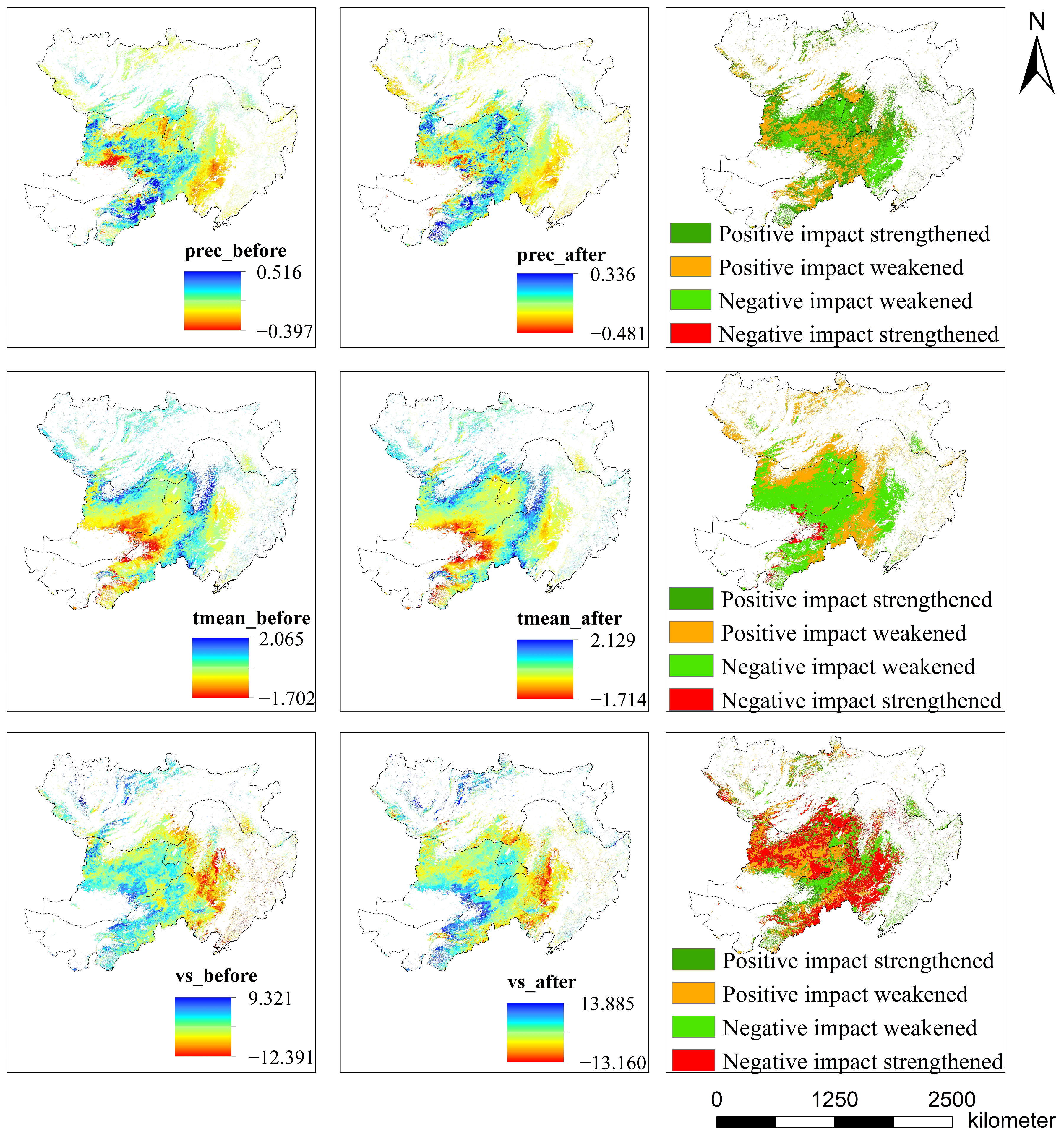
Partial correlation and multiple linear regression analyses were conducted on precipitation, average temperature, and wind speed before and after the maximum mutations. The results concluded that precipitation is the most important factor influencing GVC mutations in CMREC, with a 43% positive impact enhancement, and it is relatively continuous and stable. Wind speed, on the other hand, had a 45% negative impact, primarily in the Mongolian region and the China–Mongolia–Russia tri-border area, which was unfavorable to grassland growth. Understanding the causes of mutations in GVC will help predict future changes and impacts on vegetation ecosystems, promoting grassland ecological conservation and sustainable development in the CMREC region.

References

1. Zhao, Y.; Liu, Z.; Wu, J. Grassland ecosystem services: A systematic review of research advances and future directions. Landsc. Ecol. 2020, 35, 793–814. [Google Scholar] [CrossRef]
2. Shi, P.; Li, P.; Li, Z.; Sun, J.; Wang, D.; Min, Z. Effects of grass vegetation coverage and position on runoff and sediment yields on the slope of Loess Plateau, China. Agric. Water Manag. 2022, 259, 107231. [Google Scholar] [CrossRef]
3. Li, M.; Bai, L.; Yang, L.; Wang, Q.; Zhu, J. Amount, distribution and controls of the soil organic carbon storage loss in the degraded China’s grasslands. Sci. Total Environ. 2024, 944, 173848. [Google Scholar] [CrossRef] [PubMed]
4. Li, P.; Zhu, W.; He, B. Regional differences in the impact paths of climate on aboveground biomass in alpine grasslands across the Qinghai-Tibet Plateau. Sci. Total Environ. 2024, 947, 174421. [Google Scholar] [CrossRef]
5. Fu, L.; Bo, T.; Du, G.; Zheng, X. Modeling the responses of grassland vegetation coverage to grazing disturbance in an alpine meadow. Ecol. Model. 2012, 247, 221–232. [Google Scholar] [CrossRef]
6. Fan, Z.; Bai, R.; Yue, T.-X. Scenarios of land cover in Eurasia under climate change. J. Geogr. Sci. 2020, 30, 3–17. [Google Scholar] [CrossRef]
7. Fan, Z.; Fan, B.; Yue, T.-X. Terrestrial ecosystem scenarios and their response to climate change in Eurasia. Sci. China Earth Sci. 2019, 62, 1607–1618. [Google Scholar] [CrossRef]
8. Sternberg, T.; Rueff, H.; Middleton, N. Contraction of the Gobi Desert, 2000–2012. Remote Sens. 2015, 7, 1346–1358. [Google Scholar] [CrossRef]
9. Cleland, E.; Collins, S.; Dickson, T.; Farrer, E.; Gherardi, L.; Hallett, L.; Hobbs, R.; Hsu, J.; Turnbull, L.; Suding, K. Sensitivity of grassland plant community composition to spatial vs. temporal variation in precipitation. Ecology 2013, 94, 1687–1696. [Google Scholar] [CrossRef]
10. Gang, C.; Zhaoqi, W.; Yang, Y.; Chen, Y.Z.; Zhang, Y.; Li, J.L.; Cheng, J.M. The NPP spatiotemporal variation of global grassland ecosystems in response to climate change over the past 100 years. Acta Pratacult. Sin. 2016, 25, 1–14. [Google Scholar] [CrossRef]
11. Mu, X.; Hu, M.; Song, W.; Ruan, G.; Ge, Y.; Wang, J.; Huang, S.; Yan, G. Evaluation of Sampling Methods for Validation of Remotely Sensed Fractional Vegetation Cover. Remote Sens. 2015, 7, 16164–16182. [Google Scholar] [CrossRef]
12. Ding, Y.; Ge, Y.; Hu, M.; Zhang, H. Comparison of different spatial sampling methods for validation of GEOV1 FVC product over heterogeneous and homogeneous surfaces. In Proceedings of the Remote Sensing for Agriculture, Ecosystems, and Hydrology XVIII, Edinburgh, UK, 25 October 2016; pp. 134–143. [Google Scholar]
13. Weltz, M.; Ritchie, J.; Fox, H. Comparison of laser and field measurements of vegetation height and canopy cover. Water Resour. Res. 1994, 30, 1311–1320. [Google Scholar] [CrossRef]
14. Gao, X.; Dong, S.; Li, S.; Xu, Y.; Liu, S.; Zhao, H.; Yeomans, J.; Li, Y.; Shen, H.; Wu, S.; et al. Using the random forest model and validated MODIS with the field spectrometer measurement promote the accuracy of estimating aboveground biomass and coverage of alpine grasslands on the Qinghai-Tibetan Plateau. Ecol. Indic. 2020, 112, 106114. [Google Scholar] [CrossRef]
15. Tang, L.; He, M.; Li, X. Verification of Fractional Vegetation Coverage and NDVI of Desert Vegetation via UAVRS Technology. Remote Sens. 2020, 12, 1742. [Google Scholar] [CrossRef]
16. Du, M.; Li, M.; Noguchi, N.; Ji, J.; Ye, M. Retrieval of Fractional Vegetation Cover from Remote Sensing Image of Unmanned Aerial Vehicle Based on Mixed Pixel Decomposition Method. Drones 2023, 7, 43. [Google Scholar] [CrossRef]
17. Guo, Z.; Liu, S.; Feng, K.; Kang, W.; Chen, X. Machine Learning-Based Remote Sensing Inversion of Non-Photosynthetic/Photosynthetic Vegetation Coverage in Desertified Areas and Its Response to Drought Analysis. Remote Sens. 2024, 16, 3226. [Google Scholar] [CrossRef]
18. Weber, D.; Schwieder, M.; Ritter, L.; Koch, T.; Psomas, A.; Huber, N.; Ginzler, C.; Boch, S. Grassland-use intensity maps for Switzerland based on satellite time series: Challenges and opportunities for ecological applications. Remote Sens. Ecol. Conserv. 2023, 10, 312–327. [Google Scholar] [CrossRef]
19. Ge, J.; Meng, B.; Liang, T.; Feng, Q.; Gao, J.; Yang, S.; Huang, X.; Xie, H. Modeling alpine grassland cover based on MODIS data and support vector machine regression in the headwater region of the Huanghe River, China. Remote Sens. Environ. 2018, 218, 162–173. [Google Scholar] [CrossRef]
20. Wu, H.; An, S.; Meng, B.; Chen, X.; Li, F.; Ren, S. Retrieval of grassland aboveground biomass across three ecoregions in China during the past two decades using satellite remote sensing technology and machine learning algorithms. Int. J. Appl. Earth Obs. Geoinf. 2024, 130, 103925. [Google Scholar] [CrossRef]
21. Chen, X.; Sun, Y.; Qin, X.; Cai, J.; Cai, M.; Hou, X.; Yang, K.; Zhang, H. Assessing the Potential of UAV for Large-Scale Fractional Vegetation Cover Mapping with Satellite Data and Machine Learning. Remote Sens. 2024, 16, 3587. [Google Scholar] [CrossRef]
22. Zhang, Y.; Liu, T.; Tong, X.; Duan, L.; Jia, T.; Ji, Y. Inversion of vegetation coverage based on multi-source remote sensing data and machine learning method in the Horqin Sandy Land, China. J. Desert Res. 2022, 42, 187. [Google Scholar]
23. Yang, D.; Yang, Z.; Wen, Q.; Ma, L.; Guo, J.; Chen, A.; Zhang, M.; Xing, X.; Yuan, Y.; Lan, X.; et al. Dynamic monitoring of aboveground biomass in inner Mongolia grasslands over the past 23 Years using GEE and analysis of its driving forces. J. Environ. Manag. 2024, 354, 120415. [Google Scholar] [CrossRef] [PubMed]
24. Breiman, L. Random Forests. Mach. Learn. 2001, 45, 5–32. [Google Scholar] [CrossRef]
25. Zeng, N.; Ren, X.; He, H.; Zhang, L.; Zhao, D.; Ge, R.; Li, P.; Niu, Z. Estimating grassland aboveground biomass on the Tibetan Plateau using a random forest algorithm. Ecol. Indic. 2019, 102, 479–487. [Google Scholar] [CrossRef]
26. Wang, J.; Xiao, X.; Bajgain, R.; Starks, P.; Steiner, J.; Doughty, R.; Chang, Q. Estimating leaf area index and aboveground biomass of grazing pastures using Sentinel-1, Sentinel-2 and Landsat images. ISPRS J. Photogramm. Remote Sens. 2019, 154, 189–201. [Google Scholar] [CrossRef]
27. Kennedy, R.; Yang, Z.; Cohen, W. Detecting trends in forest disturbance and recovery using yearly Landsat time series: 1. LandTrendr—Temporal segmentation algorithms. Remote Sens. Environ. 2010, 114, 2897–2910. [Google Scholar] [CrossRef]
28. Li, M.; Huang, C.; Zhu, Z.; Shi, H.; Lu, H.; Peng, S. Assessing rates of forest change and fragmentation in Alabama, USA, using the vegetation change tracker model. For. Ecol. Manag. 2009, 257, 1480–1488. [Google Scholar] [CrossRef]
29. Jamali, S.; Jönsson, P.; Eklundh, L.; Ardö, J.; Seaquist, J. Detecting changes in vegetation trends using time series segmentation. Remote Sens. Environ. 2015, 156, 182–195. [Google Scholar] [CrossRef]
30. Verbesselt, J.; Hyndman, R.; Newnham, G.; Culvenor, D. Detecting trend and seasonal changes in satellite image time series. Remote Sens. Environ. 2010, 114, 106–115. [Google Scholar] [CrossRef]
31. Zhong, X.; Li, J.; Wang, J.; Zhang, J.; Liu, L.; Ma, J. Linear and Nonlinear Characteristics of Long-Term NDVI Using Trend Analysis: A Case Study of Lancang-Mekong River Basin. Remote Sens. 2022, 14, 6271. [Google Scholar] [CrossRef]
32. Luo, S.; Liu, H.; Gong, H. Nonlinear trends and spatial pattern analysis of vegetation cover change in China from 1982 to 2018. Acta Ecol. Sin. 2022, 42, 8331–8342. [Google Scholar] [CrossRef]
33. Schultz, M.; Clevers, J.G.P.W.; Carter, S.; Verbesselt, J.; Avitabile, V.; Quang, H.; Herold, M. Performance of vegetation indices from Landsat time series in deforestation monitoring. Int. J. Appl. Earth Obs. Geoinf. 2016, 52, 318–327. [Google Scholar] [CrossRef]
34. Li, L.; Zhang, Y.; Liu, Q.; Ding, M.; Mondal, P. Regional differences in shifts of temperature trends across China between 1980 and 2017. Int. J. Climatol. 2018, 39, 1157–1165. [Google Scholar] [CrossRef]
35. Dupas, R.; Minaudo, C.; Gruau, G.; Ruiz, L.; Gascuel-Odoux, C. Multidecadal Trajectory of Riverine Nitrogen and Phosphorus Dynamics in Rural Catchments. Water Resour. Res. 2018, 54, 5327–5340. [Google Scholar] [CrossRef]
36. Horion, S.; Ivits, E.; Keersmaecker, W.; Tagesson, T.; Vogt, J.; Fensholt, R. Mapping European ecosystem change types in response to land-use change, extreme climate events and land degradation. Land Degrad. Dev. 2019, 30, 951–963. [Google Scholar] [CrossRef]
37. Ersi, C.; Bayaer, T.; Bao, Y.; Bao, Y.; Yong, M.; Zhang, X. Temporal and Spatial Changes in Evapotranspiration and Its Potential Driving Factors in Mongolia over the Past 20 Years. Remote Sens. 2022, 14, 1856. [Google Scholar] [CrossRef]
38. Guo, E.; Wang, Y.; Wang, C.; Bao, Y.; Mandula, N.; Jirigala, B.; Bao, Y.; Li, H. NDVI Indicates Long-Term Dynamics of Vegetation and Its Driving Forces from Climatic and Anthropogenic Factors in Mongolian Plateau. Remote Sens. 2021, 13, 688. [Google Scholar] [CrossRef]
39. Wu, D.; Zhao, X.; Liang, S.; Zhou, T.; Huang, K.; Tang, B.; Zhao, W. Time-lag Effects of Global Vegetation Responses to Climate Change. Glob. Change Biol. 2015, 21, 3520–3531. [Google Scholar] [CrossRef]
40. Yiming, W.; Zhang, Z.; Chen, X. Quantifying Influences of Natural and Anthropogenic Factors on Vegetation Changes Based on Geodetector: A Case Study in the Poyang Lake Basin, China. Remote Sens. 2021, 13, 5081. [Google Scholar] [CrossRef]
41. Offiong, R.; Iwara, A. Quantifying the Stock of Soil Organic Carbon using Multiple Regression Model in a Fallow Vegetation, Southern Nigeria. Ethiop. J. Environ. Stud. Manag. 2012, 5, 166–172. [Google Scholar] [CrossRef]
42. Li, X.; Zhang, X.; Xu, X. Precipitation and Anthropogenic Activities Jointly Green the China–Mongolia–Russia Economic Corridor. Remote Sens. 2022, 14, 187. [Google Scholar] [CrossRef]
43. Shi, H.; Gao, Q.; Qi, Y.; Liu, J.; Hu, Y. Wind erosion hazard assessment of the Mongolian Plateau using FCM and GIS techniques. Environ. Earth Sci. 2009, 61, 689–697. [Google Scholar] [CrossRef]
44. Fang, J.; Bai, Y.; Wu, J. Towards a better understanding of landscape patterns and ecosystem processes of the Mongolian Plateau. Landsc. Ecol. 2015, 30, 1573–1578. [Google Scholar] [CrossRef]
45. Fan, Z.; Li, S.; Fang, H. Explicitly Identifying the Desertification Change in CMREC Area Based on Multisource Remote Data. Remote Sens. 2020, 12, 3170. [Google Scholar] [CrossRef]
46. Meng, B.; Jinlong, G.; Liang, T.; Cui, X.; Ge, J.; Yin, J.; Feng, Q.; Xie, H. Modeling of Alpine Grassland Cover Based on Unmanned Aerial Vehicle Technology and Multi-Factor Methods: A Case Study in the East of Tibetan Plateau, China. Remote Sens. 2018, 10, 320. [Google Scholar] [CrossRef]
47. Liu, Z.; Chen, Y.; Chen, C. Analysis of the Spatiotemporal Characteristics and Influencing Factors of the NDVI Based on the GEE Cloud Platform and Landsat Images. Remote Sens. 2023, 15, 4980. [Google Scholar] [CrossRef]
48. Fu, B.; Yang, W.; Yao, H.; He, H.; Lan, G.; Gao, E.; Qin, J.; Donglin, F.; Chen, Z. Evaluation of spatio-temporal variations of FVC and its relationship with climate change using GEE and Landsat images in Ganjiang River Basin. Geocarto Int. 2022, 37, 13658–13688. [Google Scholar] [CrossRef]
49. Wang, J.; Meng, S.; Zhu, W.; Xu, Z. Phenological Changes and Their Influencing Factors under the Joint Action of Water and Temperature in Northeast Asia. Remote Sens. 2023, 15, 5298. [Google Scholar] [CrossRef]
50. De Cáceres, M.; Martin-StPaul, N.; Turco, M.; Cabon, A.; Granda, V. Estimating daily meteorological data and downscaling climate models over landscapes. Environ. Model. Softw. 2018, 108, 186–196. [Google Scholar] [CrossRef]
51. Castro, W.; Junior, J.; Polidoro, C.; Osco, L.; Gonçalves, W.; Rodrigues, L.; Santos, M.; Jank, L.; Barrios, S.; Borges do Valle, C.; et al. Deep Learning Applied to Phenotyping of Biomass in Forages with UAV-Based RGB Imagery. Sensors 2020, 20, 4802. [Google Scholar] [CrossRef]
52. Karila, K.; Alves de Oliveira, R.; Ek, J.; Kaivosoja, J.; Koivumäki, N.; Korhonen, P.; Niemeläinen, O.; Nyholm, L.; Näsi, R.; Pölönen, I.; et al. Estimating Grass Sward Quality and Quantity Parameters Using Drone Remote Sensing with Deep Neural Networks. Remote Sens. 2022, 14, 2692. [Google Scholar] [CrossRef]
53. Yan, Y.; Liu, X.; Wen, Y.; Ou, J. Quantitative analysis of the contributions of climatic and human factors to grassland productivity in northern China. Ecol. Indic. 2019, 103, 542–553. [Google Scholar] [CrossRef]
54. Yang, Y.; Zhaoqi, W.; Li, J.; Gang, C.; Zhang, Y.; Zhang, Y.; Odeh, I.; Qi, J. Comparative assessment of grassland degradation dynamics in response to climate variation and human activities in China, Mongolia, Pakistan and Uzbekistan from 2000 to 2013. J. Arid Environ. 2016, 135, 164–172. [Google Scholar] [CrossRef]
55. Yan, X.; Li, J.; Shao, Y.; Hu, Z.; Yang, Q.; Shouqiang, Y.; Cui, L. Driving forces of grassland vegetation changes in Chen Barag Banner, Inner Mongolia. GISci. Remote Sens. 2020, 57, 753–769. [Google Scholar] [CrossRef]
56. Chen, L.; Li, H.; Zhang, P.; Zhao, X.; Zhou, L.; Liu, T.; Hu, H.; Bai, Y.; Shen, H.; Fang, J. Climate and native grassland vegetation as drivers of the community structures of shrub-encroached grasslands in Inner Mongolia, China. Landsc. Ecol. 2014, 30, 1627–1641. [Google Scholar] [CrossRef]
57. Zemmrich, A.; Manthey, M.; Zerbe, S.; Oyunchimeg, D. Driving environmental factors and the role of grazing in grassland communities: A comparative study along an altitudinal gradient in Western Mongolia. J. Arid Environ. 2010, 74, 1271–1280. [Google Scholar] [CrossRef]
58. Yang, H.; Auerswald, K.; Gong, X.; Schnyder, H.; Bai, Y. Climate and anthropogenic drivers of changes in abundance of C4 annuals and perennials in grasslands on the Mongolian Plateau. Grassl. Res. 2022, 1, 131–141. [Google Scholar] [CrossRef]
59. Pazur, R.; Prishchepov, A.; Mjachina, K.; Verburg, P.; Levykin, S.; Ponkina, E.; Kazachkov, G.; Yakovlev, I.; Akhmetov, R.; Rogova, N.; et al. Restoring steppe landscapes: Patterns, drivers and implications in Russia’s steppes. Landsc. Ecol. 2021, 36, 407–425. [Google Scholar] [CrossRef]
60. Matasov, V.; Prishchepov, A.; Jepsen, M.; Müller, D. Spatial determinants and underlying drivers of land-use transitions in European Russia from 1770 to 2010. J. Land Use Sci. 2019, 14, 362–377. [Google Scholar] [CrossRef]
Figure 1. Map of grassland coverage in the China–Mongolia–Russia Economic Corridor.
Remotesensing 17 01334 g001
Figure 2. Technology roadmap.
Remotesensing 17 01334 g002
Figure 3. Comparison of machine learning inversion accuracy.
Remotesensing 17 01334 g003
Figure 4. RF inversion of CMREC for GVC in 2022.
Remotesensing 17 01334 g004
Figure 5. Number of mutations of GVC.
Remotesensing 17 01334 g005
Figure 6. Percentage of number of mutations.
Remotesensing 17 01334 g006
Figure 7. Year of maximum mutations.
Remotesensing 17 01334 g007
Figure 8. Percentage of years with maximum mutations.
Remotesensing 17 01334 g008
Figure 9. Month of maximum mutations.
Remotesensing 17 01334 g009
Figure 10. Percentage of months with maximum mutation.
Remotesensing 17 01334 g010
Figure 11. Magnitude of mutations.
Remotesensing 17 01334 g011
Figure 12. Percentage of mutation magnitude.
Remotesensing 17 01334 g012
Figure 13. Percentage of mutation magnitude in different years.
Remotesensing 17 01334 g013
Figure 14. Percentage of mutations magnitude in different months.
Remotesensing 17 01334 g014
Figure 15. Spatial distribution of VIF values for the three climate factors.
Remotesensing 17 01334 g015
Figure 16. Partial correlation coefficients of drivers before and after the maximum mutations and their trends.
Remotesensing 17 01334 g016
Figure 17. Multiple linear regression coefficients of drivers before and after the maximum mutations and their trends.
Remotesensing 17 01334 g017