Enhancing Urban Flood Susceptibility Assessment by Capturing the Features of the Urban Environment

Abstract

The frequent occurrence of urban floods (UFs) poses significant threats to public safety and the national economy. Accurate estimation of urban flood susceptibility (UFS) and the identification of potential hotspots are critical for effective UF management. However, existing UFS studies often fall short due to a limited understanding of UFs’ nature, frequently relying on disaster factors analogous to those used for natural floods while neglecting key urban characteristics, limiting the accuracy of UFS estimates. To address these challenges, we propose a novel framework for UFS assessment. Unlike those studies that focus primarily on topographic and surface characteristics, our approach integrates urban-specific factors that capture the distinctive attributes of the urban environment, including Urban Heat Island Intensity, Urban Rain Island Intensity, Urban Resilience Index, and Impervious Surface Percentage. Guangzhou was selected as the study area, where machine learning methods were employed to calculate UFS, and Shapley Additive Explanation was utilized to quantify the contributions of employed factors. We evaluated the significance of urban factors from three perspectives: classifier performance, map accuracy, and factor importance. The results indicate that (1) urban factors hold significantly greater importance compared to other factors, and (2) the incorporation of urban factors markedly enhances both the performance of the trained classifier and the accuracy of the UFS map. These findings underscore the value of integrating urban factors into UFS assessments, thereby contributing to more precise UF management and supporting sustainable urban development.

1. Introduction

Urban floods (UFs) occur due to the insufficient capacity of urban drainage systems combined with heavy rainfall, leading to significant water accumulation in urban areas [1]. With the accelerating impacts of climate change and rapid urbanization, UFs have become increasingly severe in developing countries over recent decades, resulting in substantial casualties and economic losses. Since 2010, over 180 cities in China have been affected by UFs annually, causing direct economic losses exceeding USD 14 billion [2]. For instance, an extreme rainstorm struck the Beijing-Tianjin-Hebei region on 23 July 2023, impacting more than five million people and leading to direct economic losses of over USD 13 billion. Therefore, addressing UF challenges and mitigating associated losses remains a critical and urgent issue.

Among the various UF management tasks, effective UF prediction is paramount; susceptibility assessment, which identifies potential UF hotspots, is a key component of prediction works [3]. The methodology used for evaluating urban flood susceptibility (UFS) is crucial, as it directly influences the spatial pattern and precision of the results [4]. Current studies evaluate the UFS are predominantly derived from hydrological and geographical approaches [5]. Hydrological approaches utilize physical models to simulate the spatial distribution of inundated areas based on the principles of water movement, with representative models including the Storm Water Management Model [6] and the Stormwater Investment Planning and Selection Optimization Network [7]. Although physical models can accurately depict the spatial distribution of UFS in localized areas [8], the required driving data for such methods are often difficult to obtain [9], making these models challenging to generalize to large-scale study areas [10,11].

Geographical approaches, on the other hand, infer UFS hotspots based on the influence of disaster-causing factors, as exemplified by indicator-based and machine learning (ML) methods. The indicator-based method, represented by the Analytic Hierarchy Process [12] and Principal Component Analysis [13], evaluates UFS through the calculation of a weighted sum based on identified disaster factors [14]. While indicator methods can efficiently assess UFS using readily available data, they lack the ability to optimize and refine the estimated values against actual observed data, often resulting in lower accuracy [15]. In contrast, ML methods leverage observed flooded locations and environmental variables to accurately model the nonlinear relationships between disaster factors and UFs, leading to more objective and precise UFS assessments [16]. Due to these advantages, ML models, such as Extreme Gradient Boosting (XGBoost) [17], Support Vector Machine (SVM) [18], and Random Forest (RF) [19], have become increasingly prevalent in large-scale UFS studies.

Currently, most ML-based UFS studies focus on enhancing assessment accuracy by improving model performance [20,21] and optimizing training samples [22,23]. However, this emphasis on methodological improvements often overlooks a deeper understanding of the inherent nature of UFs. Specifically, there is a frequent conflation between UFs and natural floods (NFs), despite their fundamental differences. NFs are typically triggered by river breaches or coastal dam failures, with water sources primarily originating from natural waters, leading to passive inundations [24]. In NFs, natural factors like topography significantly influence the NFs’ spatial spread, while human factors play a relatively minor role [25]. In contrast, UFs are primarily caused by heavy rainfall and the failure of drainage systems, leading to active inundation. The spatial heterogeneity of UFS is mainly influenced by the urban environment [26]. Thus, unlike NFs, UFs occur within urban environments and exhibit more pronounced anthropogenic characteristics. Despite this, many current UFS studies utilize indicators like those in NF research [27,28]. For example, Tehrany et al. only added LULC to describe human activities in addition to natural factors [29]. Rahmati et al. only chooses elevation, distance from the river, and other natural factors for UFS [30]. Consequently, the factors used in these studies often fail to fully capture the distinct nature of UFs. While recent studies have incorporated the impervious surface (a critical parameter characterizing urban morphology) into UFS evaluations [31,32], the singular dependence on this metric inadequately captures the comprehensive response mechanisms of urban systems to UFs.

Collectively, previous ML-based UFS studies lacked a mature understanding of the anthropogenic attributes of UFs, leading to deficiencies in the constructed spatial databases and, consequently, limiting the accuracy and objectivity of UFS simulations. To address that challenge, this study enhances the disaster factors in the spatial database by introducing indicators that capture the multidimensional attributes of urban environments. Guangzhou, China, was selected as the study area. UFS was assessed using ML methods, and the contribution of driving factors was quantified using Shapley Additive Explanation (SHAP). The research objectives were to (1) enhance the UF spatial database, (2) simulate the UFS distribution, and (3) underscore the significance of urban factors. We believe the proposed framework offers a novel perspective for improving the precision of UFS assessments, thereby providing effective decision-making support for UF prevention and promoting sustainable development in developing countries.

2. Study Area and Data

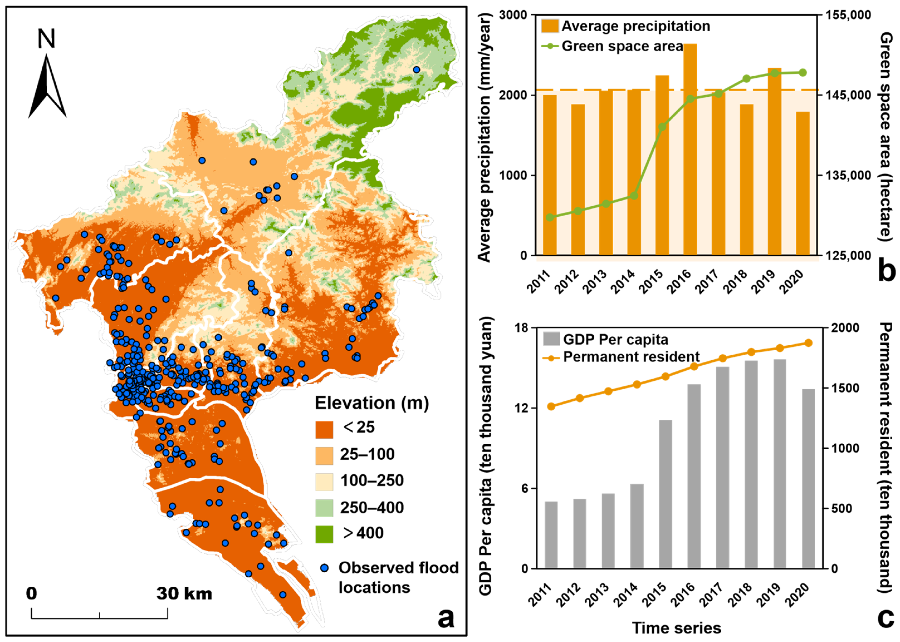
2.1. Study Area

Guangzhou is situated between 112°6′ and 114°3′E and between 22°26′ and 23°56′N, covering an area of over 7430 km² (see Figure 1). Guangzhou experiences a subtropical monsoon climate, with an average annual temperature ranging from 20 to 22 °C. Statistical documents from 2011 to 2020 indicate that the average annual precipitation in Guangzhou is approximately 2090 mm, with heavy rainfall occurring from April to September. The city is endowed with substantial vegetation resources, encompassing more than 100,000 hectares of green space; the total green area increased by 13.9% from 2011 to 2020. Over the past two decades, Guangzhou has undergone rapid urbanization, with the urbanization rate rising from 71.6% in 2000 to 80.5% in 2020. This swift urban expansion has introduced extensive impervious surfaces, exacerbating the city’s vulnerability to UF due to the combination of its natural high temperatures and rainy climate. Recent rainstorm and flood events on 7 May 2017 and 22 May 2020 have had a significant impact on residents and resulted in substantial economic losses. For the above reasons, Guangzhou was an outstanding representative which we selected as the study region.

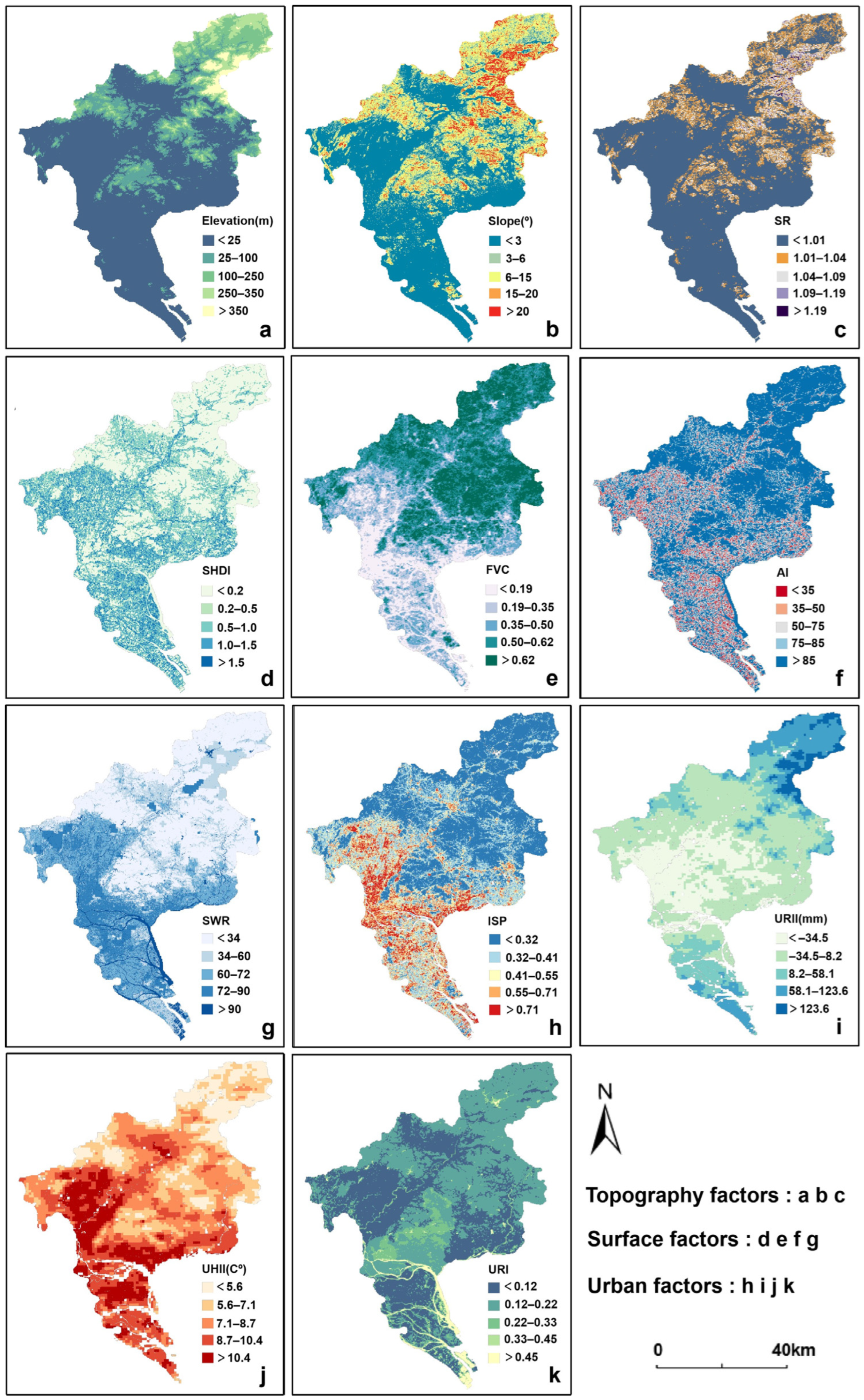
2.2. UF Spatial Database

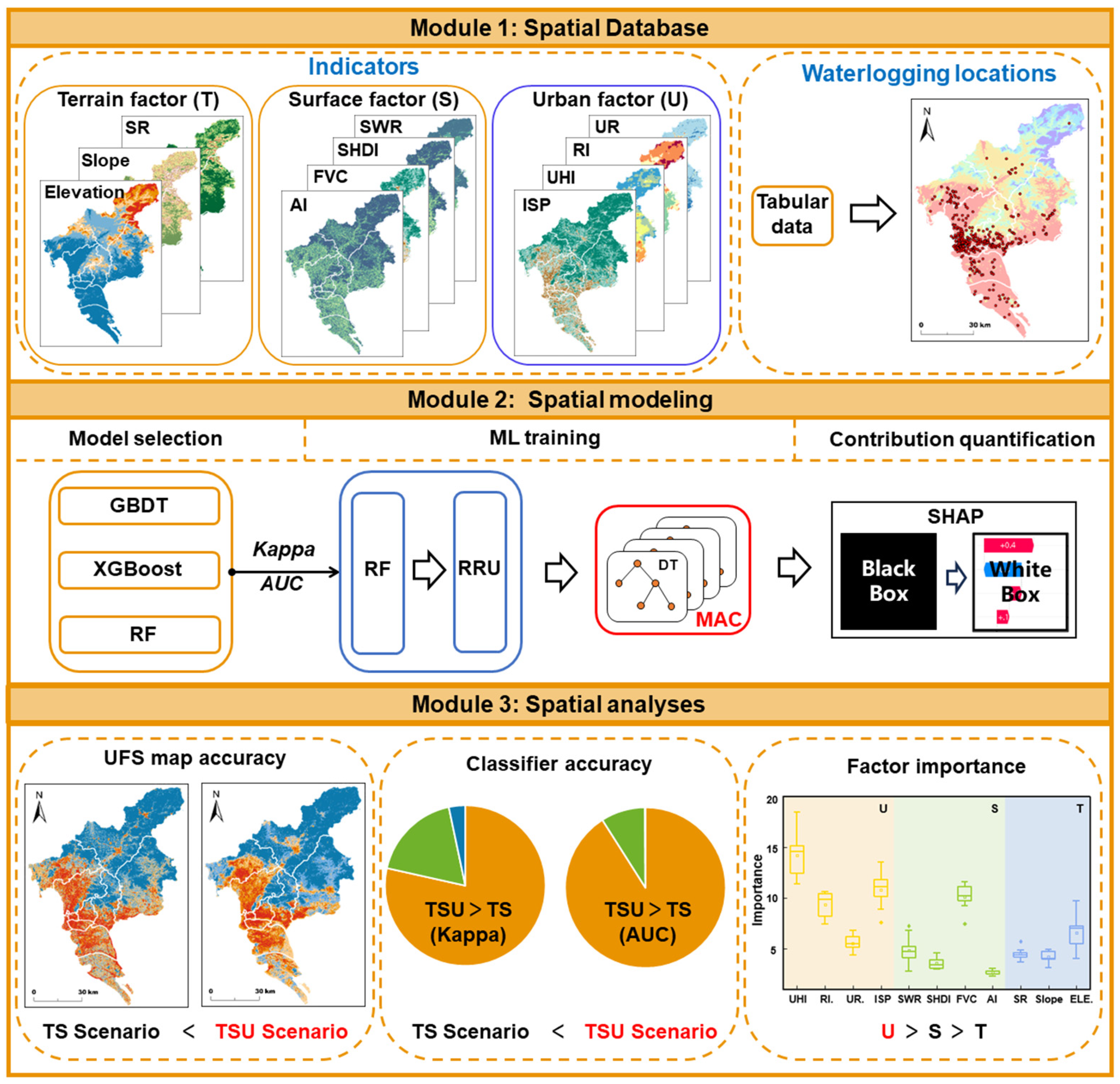
The UF spatial database in this study comprises observed flood locations and disaster factors, all derived from open sources (see Table S1). Observed flood locations are obtained from the Guangzhou Water Affairs Bureau’s 2020 report on flood-prone areas, which has been converted into shapefile data representing the spatial distribution of these locations, 488 in total. To account for both natural and anthropogenic influences on UFs, and based on recommendations from relevant studies [33,34,35], we selected 11 factors for UFS evaluation; these factors are categorized into three major groups: topographic, surface, and urban factors.

Topographic and surface factors are widely utilized indicators in current UFS studies. Topographic factors encompass elevation, slope, and Surface Roughness (SR) (see Figure 2a–c); they generally influence the direction and velocity of water flow, thereby significantly impacting the formation of inundated areas [36]. For more detailed definitions and calculation methodologies of the above indicators, refer to the Supplementary Materials.

Surface factors include the Shannon Diversity Index (SHDI), Fractional Vegetation Coverage (FVC), Aggregation Index (AI), and Soil Water Retention (SWR) (see Figure 2d–g); they affect UF by modulating surface water infiltration and runoff generation [37]. For more detailed definitions and calculation methodologies of the above indicators, refer to the Supplementary Materials.

Urban factors are novelly introduced in this study to capture urban characteristics, including Impervious Surface Percentage (ISP), Urban Rain Island Intensity (URII), Urban Heat Island Intensity (UHII), and the Urban Resilience Index (URI) (see Figure 2h–k). These factors collectively reflect the impact of human activities on urban environments, demonstrating significant relevance to UFS [38]. ISP has been extensively validated in numerous studies as a critical determinant of surface water infiltration capacity, directly influencing UFS [39]. Both UHII and URII alter microclimates across different urban areas, thereby affecting rainfall distribution between central and peripheral regions, which in turn influences the spatial distribution of UFS [40]. The URI quantifies the vulnerability and resilience of the urban environment to flood events, thereby enhancing the comprehensiveness of UFS assessments [41]. For more detailed definitions and calculation methodologies of the above indicators, refer to the Supplementary Materials.

The factors influencing UFS interact through complex, multidimensional mechanisms. Topographic factors directly regulate flow direction, velocity, and water accumulation, while surface factors modulate runoff and infiltration. Urban factors reflect human activities’ impact on flood dynamics. Additionally, the combined influence of topography, surface characteristics, and urbanization can amplify UFS in specific areas. Understanding these interactions is critical for developing robust flood mitigation strategies and informed urban planning, as they collectively shape the spatial distribution and severity of UFs.

3. Methodology

To address the issue of incomplete disaster factors in current UFS studies, we introduce a novel UF spatial database that integrates both natural and anthropologic attributes of UF, aiming to enhance UFS evaluation by incorporating muti-dimensional indicators. The spatial framework is organized into the following three modules: Spatial Database, Spatial Modeling, and Spatial Analyses (see Figure 3).

Spatial Database Module: The database comprises 11 factors representing topography, surface, and urban domains, along with 488 observed flood locations. Through preprocessing, all factors were standardized to the same spatial extent, coordinate system, and spatial resolution (30 m × 30 m).

Spatial Modeling Module: Three widely used ML models—Gradient Boosting Decision Tree (GBDT), XGBoost, and RF—were selected for comparison, with the model demonstrating the highest accuracy chosen as the basis for UFS evaluation. The Repeated Random Undersampling (RRU) technique was employed to select high-quality negative samples, which were then used to train the Most Accurate Classifier (MAC) for generating UFS Maps (UFSMs). The SHAP method was utilized to quantify the contribution of each factor from both global and local perspectives.

Spatial Analysis Module: The importance of urban factors was assessed by comparing two scenarios: (1) the TSU scenario: including topographic, surface, and urban factors, and (2) the TS scenario: including only topographic and surface factors. This comparison was conducted across multiple dimensions, including factor contributions, the UFSM precision, and classifier performance. The following sections provide a detailed explanation of the methods used and the rationale behind their selection.

3.1. UFS Evaluation

Tree-based models offer several advantages, including the ability to handle nonlinear relationships [42], robust performance in the presence of missing and outlier data [43], and the capacity to provide feature importance evaluations [33]. Consequently, these models have been widely applied in flood-related studies [44,45,46]. In this study, GBDT, XGBoost, and RF are employed to estimate UFS.

• GBDT

GBDT is an ensemble learning algorithm in ML that integrates Decision Trees (DTs) with Gradient Boosting techniques. The GBDT algorithm is distinguished by its high predictive accuracy, its effectiveness in managing both continuous and discrete data, and its ability to mitigate the impact of noisy data [31]. The GBDT model can be represented as follows:

$$F_M(x)=\sum _{m=1}^{M}T(x;{\mathit{\Theta }}_m)$$

(1)

where $T(x;{\mathit{\Theta }}_m)$ represents a Decision Tree, ${\mathit{\Theta }}_m$ denotes the parameters of the Tree, and $M$ stands for the number of DTs. The model parameters are shown in

Table 1. Machine learning model parameters.

Model	Parameter Name	Parameter Value
RF	n_estimators: Number of trees	500
	max_depth: Maximum depth of trees	default value
	max_features: Maximum number of features to consider when finding optimal split	3
GBDT	n_estimators: Number of trees	500
	max_depth: Maximum depth of trees	default value
	max_features: Maximum number of features to consider when finding optimal split	3
XGBoost	n_estimators: Number of trees	500
	max_depth: Maximum depth of trees	default value
	max_features: Maximum number of features to consider when finding optimal split	3
	colsample_bytree: Proportion of features used in each tree	0.33

.

2.

XGBoost

XGBoost, an advancement of Gradient Boosting Machine, enhances the Gradient Boosting algorithm by automating the optimization of Decision Tree (DT) sequences to minimize errors. It incorporates distributed computing methods to improve computational efficiency, applies regularization techniques to prevent overfitting and enhance model generalization, and demonstrates robustness against nonlinearity. Additionally, XGBoost features intrinsic feature selection and interpretability [31,32]. The XGBoost model can be represented as

$$\widehat{y}=\mathit{Ø}(x_i)=\sum _{k=1}^k{f}_k\left(x_i\right)$$

(2)

where $x_i$ denotes the ith sample, ${\widehat{y}}_i$ denotes the prediction value of the ith sample $x_i$, $f_k$ denotes the Kth regression tree, and K denotes the number of regression trees. The model parameters are shown in Table 1.

3.

RF

RF is an ensemble ML model comprising multiple DTs, applicable to both classification and regression tasks. It evaluates the importance of individual susceptibility indicators. Both empirical and theoretical research demonstrate that RF offers high predictive accuracy, robustness against outliers and noise, and effective overfitting prevention [47]. During the prediction phase for classification problems, each Decision Tree provides a class prediction according to the following formula:

$$\stackrel{̑}{y}={\mathit{argmax}}_c\sum _{i=1}^N{\mathit{\Omega }}_i\cdot I\left(y_i=c\right)$$

(3)

where $\stackrel{̑}{y}$ represents the final prediction result, $N$ is the number of DTs, ${\mathit{\Omega }}_i$ is the weight of the $i^{th}$ DT, $y_i$ is the prediction result of the $i^{th}$ DT, $c$ is the class, and $I(\cdot )$ is the indicator function. According to the formula above, each DT produces a voting result. The final predicted outcome is determined by the majority vote, representing the most frequent class among all the DTs’ predictions. The model parameters are shown in Table 1.

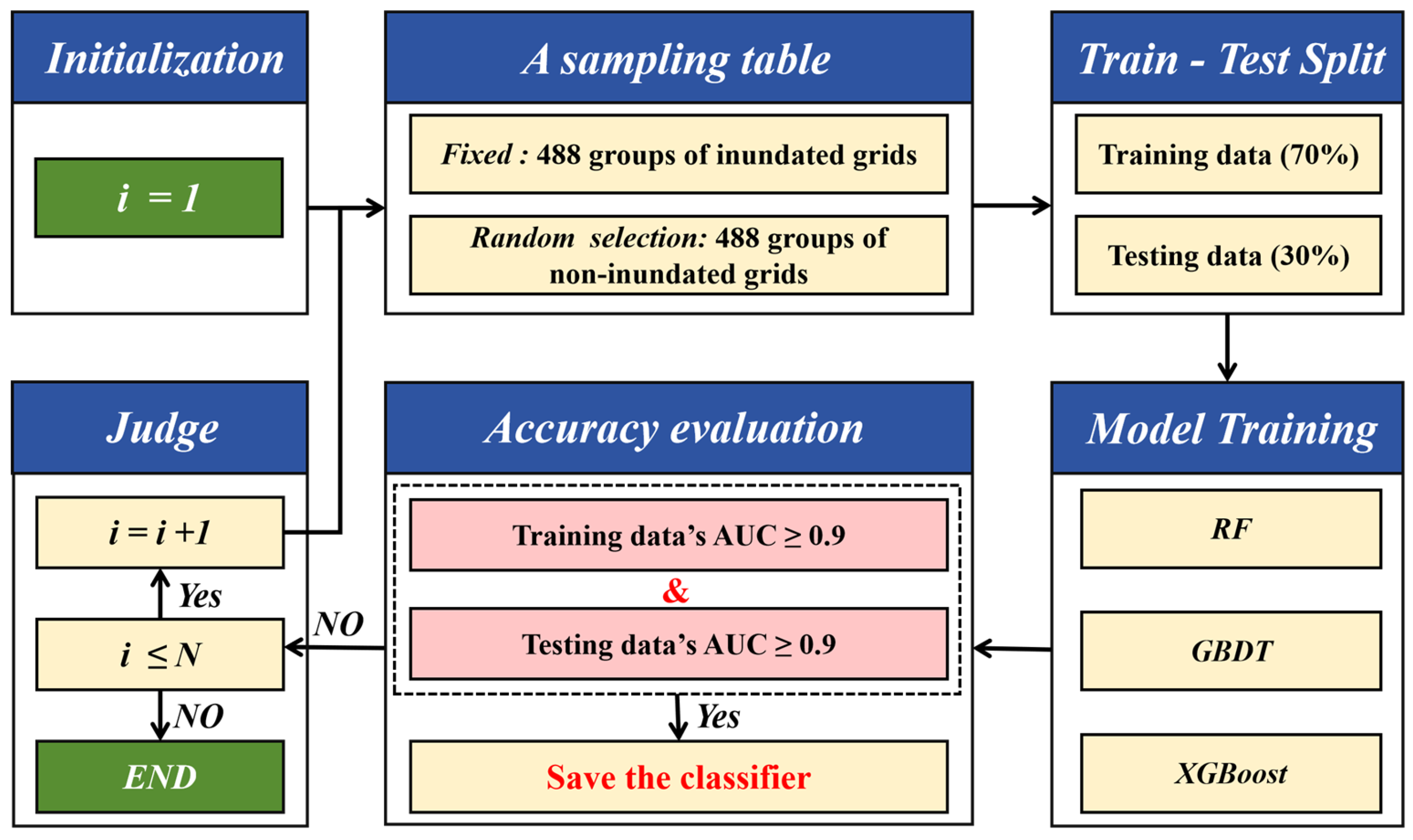
3.2. Negative Sample Screening

Balancing positive and negative samples is crucial for training the MAC. In flood datasets, negative samples are typically obtained by undersampling regions without UF reports. To ensure the quality of these samples, the RRU method was used for negative sample selection [48]. The method works for selecting the negative samples with high quality, thus obtaining a MAC for mapping the UFS distribution.

Figure 4 shows the flowchart of the sampling and verifying model used to output a MAC. In the model, N represents the number of iterations. In each sampling table, the sampling and verifying model randomly selected 488 groups of non-inundated (negative) samples to form a sampling table with 488 groups of inundated (positive) samples, and we set that 70% samples in a sampling table were randomly selected to compose the training data used to train the SVM classifier; the remaining 30% of the table formed the testing data used to verify the classification accuracy of the trained SVM classifier. To guarantee the classification accuracy of the trained classifier, the AUC coefficient was selected as the evaluation indicator and was assigned a value of 0.9 as a threshold for verifying the classifiers. Meanwhile, to guarantee the generalization capacity of the classifier, we set another rule that a classifier can be output only when the AUC values of the training data and testing data are both >0.9. In this study, N was set to 1000. After N iterations, the sampling and verifying model exported some classifiers that met the evaluation of requirements. In general, the MAC is usually selected according to the principle of both the highest AUC values of training data and testing data.

3.3. Quantification of Factors’ Contributions

ML is often regarded as a “black box” approach [49]. To better understand the relationship between factors and UFS, SHAP values are used to quantify the contributions of these factors within ML. The SHAP method is a technique for interpreting the contributions of features in ML models. It allows for the quantification of both global and local contributions [50,51], facilitating further quantitative analysis and deeper insights into how these factors impact UFS. Specifically, a larger absolute SHAP value indicates a greater contribution of the factor, while the sign of the SHAP value (positive or negative) reflects whether the factor promotes or inhibits UFS. Based on SHAP for explaining the prediction value ${\widehat{y}}_i=g\left(x_i\right)$ of the $i^{th}$ sample in the model, the calculation formula is as follows:

$${\widehat{y}}_i=y_{base}+f(x_i^{\left(1\right)})+\cdots +f(x_i^{\left(j\right)})+\cdots +f(x_i^{\left(K\right)})$$

(4)

where $x_i^{\left(j\right)}$ represents the ${ j}^{th}$ feature of the $i^{th}$ sample, $y_{base}$ is the SHAP base value, and $f(x_i^{\left(j\right)})$ denotes the Shapley value of the $j^{th}$ feature of the $i^{th}$ sample.

4. Results and Analyses

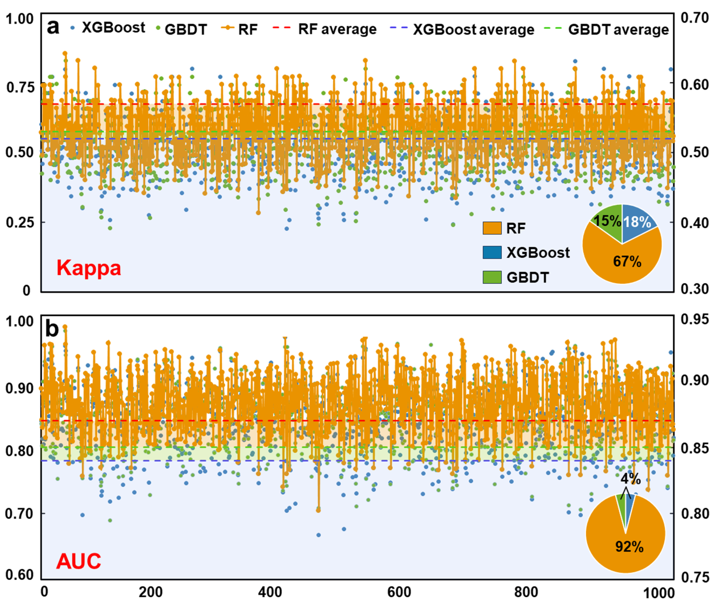
4.1. Comparisons of ML Results

Prior to model construction, a multicollinearity diagnostic was conducted for all selected factors to ensure the robustness and reliability of the model. By calculating the Tolerance and Variance Inflation Factor (VIF), the multicollinearity among the factors was comprehensively assessed. The results indicated that the Tolerance values for all factors exceeded the threshold of 0.1, and the VIF values were below 10 (see

Table 2. Multicollinearity analysis.

Variables	DEM	Slope	SR	FVC	AI	SHDI	SWR	ISP	UHI	RI	UR
Tolerance	0.370	0.112	0.138	0.205	0.257	0.222	0.421	0.352	0.238	0.368	0.740
VIF	2.702	8.929	7.269	4.870	3.897	4.505	2.376	2.840	4.195	2.714	1.351

), both metrics consistently confirming the absence of severe multicollinearity. Additionally, the correlation coefficient matrix revealed no high correlations (e.g., |r| > 0.8) among the factors. These findings collectively suggest that the selected factors are statistically independent and suitable for subsequent UFS evaluation modeling. This step helps to mitigate model bias caused by multicollinearity, thereby enhancing the accuracy and interpretability of the predictive outcomes. This rigorous diagnostic process lays the foundation for unbiased model training, allowing us to proceed with confidence to the next critical step: selecting the optimal ML for UFS evaluation.

Subsequently, we compared the performance of RF, XGBoost, and GBDT. To ensure a robust comparison, we conducted 1000 iterative samplings; in each iteration, 488 negative samples were randomly selected along with positive samples to form the dataset. We used 70% of the data for training the ML classifiers, while the remaining 30% were used for evaluating classifier performance. Kappa and AUC were employed as evaluation metrics. Figure 5a illustrates the Kappa values across the 1000 iterations: (1) The average Kappa value for RF was 0.645, exceeding the 0.612 and 0.611 averages for XGBoost and GBDT, respectively. (2) RF achieved higher Kappa values in over 67% of the iterations. Figure 5b displays the AUC values across the 1000 iterations: (1) The average AUC value for RF was 0.901, which was substantially higher than XGBoost’s 0.882 and GBDT’s 0.881. (2) RF’s AUC values surpassed those of the other methods in more than 92% of the iterations. These results demonstrate RF outperforms both XGBoost and GBDT, leading us to select RF as the foundation for UFS mapping in this study.

With RF established as the optimal algorithm, we systematically compared the classification performance between the MAC optimized by RRU and the MAC generated by Single Random Undersampling (SRU). In 1000 identical sample tests, the average Kappa value of the optimal MAC selected by RRU was 0.72, whereas SRU achieved 0.66 (see Figure 6). Moreover, the RRU-selected MAC outperformed the SRU-selected MAC in 82.1% of cases for Kappa values and 69.7% for AUC values. This demonstrates RRU’s significant advantages in both classification consistency and discriminative ability, particularly in addressing class imbalance and enhancing model reliability. Together with the preceding multicollinearity diagnostics and algorithm selection, this comprehensive approach ensures our final UFS model delivers both accuracy and interpretability.

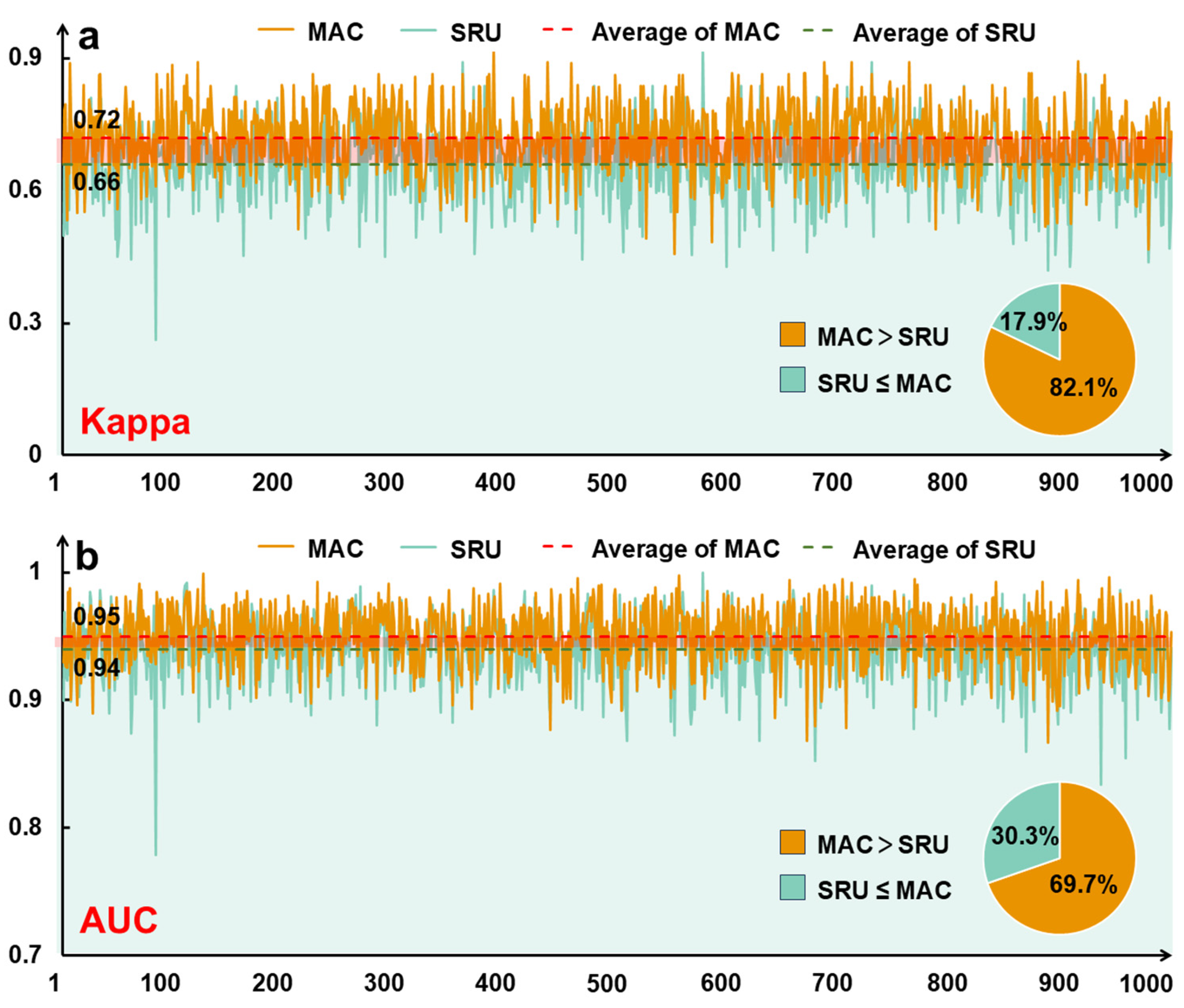
4.2. Comparisons of the TS and TSU Scenarios

First, we compared the classification performance of the generated classifiers under two scenarios. We performed 1000 iterative samplings; in each iteration, 488 negative samples were randomly selected along with positive samples to construct the dataset; 70% of the data were used to train the RF classifier, while the remaining 30% were used to evaluate classifier performance. Kappa and AUC were employed as evaluation metrics. Clearly, the Kappa values for the TSU scenario are generally higher than those for the TS scenario, with the TSU scenario surpassing the TS scenario in 81.8% of the iterations (see Figure 7a). The AUC values for the TSU scenario are significantly higher than those for the TS scenario, with the TSU scenario exceeding the TS scenario in 91.0% of the iterations (see Figure 7b). These results indicate that the classifiers generated under the TSU scenario demonstrate a markedly superior classification performance compared to the those under the TS scenario.

Next, we examined the quantification of the factors’ contributions. Using the SHAP method, we calculated both the global and local contributions (see Figure 7c,d) of the factors according to the “game rule” provided by the RF model. It is evident that, compared to topographic and surface factors, urban factors exhibit a significantly higher overall influence on UFS. Specifically, three of the top five factors with the greatest influence are urban factors. Consequently, these results underscore the superior importance of urban factors in UFS modeling. Meanwhile, SHAP, as an interpretable model, can help explain how the features of individual samples influence the model’s prediction outcomes, enhancing the transparency of model decision-making. In the waterfall plot, features with positive contributions increase the predicted value, typically represented in red, while features with negative contributions decrease the predicted value, usually shown in blue.

As shown in Figure 7, this study compares the influencing factors between high- and low-susceptibility urban flooding areas using SHAP values. In high-susceptibility areas (Figure 7e), urban factors dominate the top contributors, with UHII exhibiting the strongest positive impact, followed by FVC and ISP. Conversely, in low-susceptibility areas (Figure 7f), urban factors remain significant, but UHII, FVC, and ISP reduce flooding susceptibility. Notably, both regions reveal a synergistic interaction among UHII, ISP, and FVC, suggesting their combined role in exacerbating or mitigating flood susceptibility. These findings highlight the need to optimize urban thermal environments, enhance vegetation cover, and regulate impervious surfaces to effectively manage UFS.

Finally, we compared the generated UFSMs from the two scenarios. The RRU was employed to generate corresponding factors based on these scenarios, leading to the creation of respective MACs used to produce the UFSMs (see

Table 3. Precision of UFSMs of the TSU and TS scenarios.

Abbreviation	Kappa	AUC
TSU Scenario	0.868	0.864
TS Scenario	0.807	0.829

). The Natural Breaks method was applied to categorize the UFSMs into five levels, ranging from Very Low to Very High susceptibility. While the overall UFS patterns in both scenarios exhibit similar macro trends, local variations are evident; notably, the salt-and-pepper effect is more pronounced in the TS scenario compared to the TSU scenario (see Figure 8a,b). To quantify this, we calculated the fragmentation index for the five susceptibility levels (see Figure 8c) and observed that the average UFSM fragmentation in the TSU scenario was 0.22, lower than the 0.24 observed in the TS scenario. Generally, a lower fragmentation index indicates better spatial connectivity, suggesting a more cohesive spatial trend, which is advantageous for decision support formulation [52]. The proportion of positive samples in the UFSMs serves as a proxy for map accuracy [53]; a higher proportion implies greater accuracy. Following this logic, we found, compared with the TS scenario, that although the area percentage of the Very High susceptibility level in the UFSMs is smaller in the TSU scenario (~15% vs. ~8%) (see Figure 8c), the percentage of positive samples within these regions is notably higher (~45% vs. ~64%) (see Figure 8d). These results collectively indicate that the UFSM generated under the TSU scenario exhibits a significantly higher accuracy compared to that from the TS scenario.

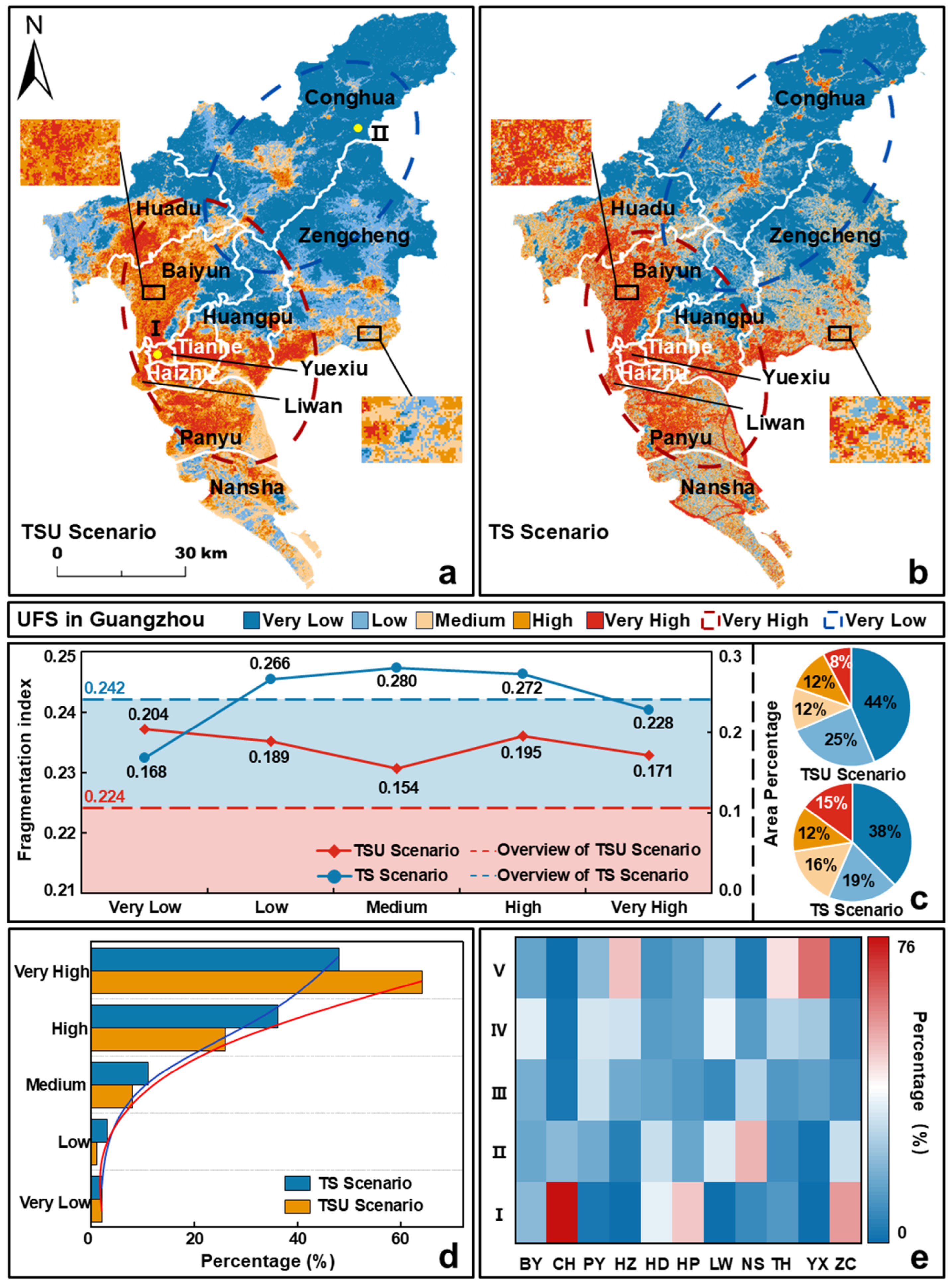
4.3. Spatial Analyses

We then analyzed the UF severity in Guangzhou based on the UFSMs and factor contribution results from the TSU scenario. The overall UFS in Guangzhou is high in the west and south while it is low in the east and north; hotspots are predominantly concentrated in the central regions, while low-susceptibility areas are mainly situated in the northern parts (see Figure 8b). Based on the area percentage of each susceptibility level, we categorize Guangzhou’s counties as follows (see Figure 8e): High-susceptibility counties (area percentage of the High and Very High susceptibility regions (s) > 60%): Yuexiu (~85%), Haizhu (~79%), and Tianhe (~70%). These counties are in the central Guangzhou, characterized by flat terrain, dense development, and sparse vegetation, which heightens their vulnerability to UF. Medium-susceptibility counties (30% < s < 60%): Liwan (~59%), Panyu (~51%), and Baiyun (~48%). These counties, which are near the central urban area, feature flat terrain and have experienced rapid urbanization in recent years, resulting in a moderate UF susceptibility. Low-susceptibility counties (s < 30%): Zengcheng (~8%), Conghua (~15%), Nansha (~16%), Huadu (~22%), and Huangpu (~26%). These areas, located on the edge of Guangzhou, have rugged terrain, lower building density, and abundant blue–green structures, contributing to a lower UF susceptibility.

Based on the SHAP values of the factors presented in Figure 7d, we found the following: Surface and Terrain Factors: Elevation (4th) and FVC (2nd) have significant impacts on UFS; elevation influences the movement of surface water bodies, while FVC reflects the density of vegetation. Urban Factors: UHII (1st) and ISP (3rd) exert the greatest influence; UHII is associated with the primary trigger of UF—precipitation—while ISP directly affects surface water infiltration. Overall, urban factors have the most pronounced impact on UFS modeling, with terrain and surface factors showing a comparable but lesser influence. Among urban factors, UHII, URII, and ISP all show positive correlations with UFS (see Figure 7d), indicating that increases in Heat Island Effects, Rain Island Effects, and Impervious Surface Coverage exacerbate UF severity. Conversely, urban resilience exhibits a negative correlation with UFS (see Figure 7d), suggesting that enhanced resilience mitigates UF susceptibility. These findings align with the expected mechanisms of these factors on UF.

5. Discussion

5.1. Implications of This Study

Accurately assessing UFS is crucial for the effective prevention of UF and the promotion of sustainable urban development. Previous research has primarily focused on enhancing the UFS precision through technical approaches like ML model selection and sample optimization [21,22]. However, many current studies tend to conflate UFs with NFs, relying heavily on disaster factors traditionally associated with NFs, i.e., topographic and surface factors, to calculate UFS. Unlike NFs, UFs are urban disasters that occur within human settlements, making the absence of indicators reflecting urban-specific characteristics a significant limitation in accurately modeling UFS.

Facing the above challenges, we introduced innovative urban factors—ISP, UHII, URII, and URI—that reflect the unique characteristics of the urban environment into the UF spatial database. To demonstrate the advantages of incorporating these urban factors, we conducted a comparative analysis between the TSU scenario (with urban factors) and the TU scenario (without urban factors). The significance of including urban factors was evaluated through classifier performance, factor importance, and map precision (see Section 4.2 for more details). The results indicated that integrating urban factors can significantly improve the UF spatial database, offering a novel perspective in enhancing UFS studies.

The UFSMs generated under the TSU scenario revealed a spatial distribution pattern of UFS in Guangzhou characterized by higher susceptibility in the west and south and lower susceptibility in the east and north. The hotspots were predominantly concentrated within the central zones; this distribution pattern aligns with the findings of previous UF susceptibility assessments in Guangzhou by [54,55]. The analysis of factor contributions highlighted the significant impact of urban factors on UF, with UHI exerting the strongest influence, consistent with the strong correlation between UHI and UF observed in [56]. These findings suggest that the simulated UFS results are reliable; thus, the identified areas of Very High susceptibility, along with the main driving factors, can provide valuable insights for effective UF management in Guangzhou.

5.2. Policy Implications for Urban Flood Management

In this study, UFS assessment successfully identified high-susceptibility areas of UFs in Guangzhou, providing a scientific basis for government departments to optimize resource allocation and implement targeted flood prevention measures in key regions. The waterfall plot of the SHAP model can determine the contribution of each factor in each local area and the main influencing factors in each local area (see Figure 7e,f), which provides decision support for effectively alleviating urban floods.

When terrain factors constitute the dominant influencing factor in a given region, the following measures should be prioritized: drainage pipe networks can be upgraded to improve rainwater drainage efficiency in areas with low terrain, where it is easy to collect rainwater [57]; in areas with steep slopes, soil and water conservation measures, like vegetation cover and terracing, should be strengthened to slow surface runoff rates [58].

When surface factors emerge as the primary determinant, implementation strategies should include increasing vegetation coverage, expanding urban green infrastructure [59], promoting rooftop greening [60], and optimizing surfaces using permeable materials [61].

When urban factors constitute the dominant influencing factor in a given region, the following measures should be prioritized: To address urban flooding caused by excessively high ISP, we need to reduce the proportion of impervious surfaces, optimize building and road layouts, and construct sponge cities through measures such as increasing permeable paving [61]. Government departments need to scientifically plan urban layouts and construct ventilation corridors to promote air circulation and disperse rainfall clouds, thereby mitigating the Urban Heat Island Effect and reducing Rain Island phenomena [62,63]. Additionally, we can leverage remote-sensing technology and meteorological monitoring networks to dynamically track changes in Urban Heat Islands and Rain Islands. By establishing early warning systems, timely response measures can be implemented [64].

5.3. Limitations and Prospects

Although the proposed urban factor set offers a novel perspective for the precise assessment of UFS, several issues remain that require attention in future research.

First, while most of the data we used had a resolution of 30 m, the data sources for calculating UHII and URII were limited to a resolution of only 1 km. This discrepancy in resolution constrains the further refinement and accuracy of UHII and URII distribution. To overcome this limitation, future research should consider use higher-resolution data sources for UHII and URII, thereby enabling the construction of a more precise UF spatial database.

Second, while we focused on enhancing UFS precision through the addition of urban factors from a spatial perspective, the impact of this framework on temporal aspects has yet to be thoroughly explored. To address this gap, future research should prioritize the collection and analysis of long-term observational data to elucidate the temporal trends of UFS, enabling more precise identification of UF hotspots.

6. Conclusions

This study presents a new perspective enhancing the accuracy of UFS assessment. Taking Guangzhou as the study case, 11 factors that capture the natural and human features of UF were selected, including the topographic, surface, and urban factors. Three ML methods, RF, XGBoost, and GBDT, were used to estimate the UFS. RRU was used to select high-quality negative samples to train a MAC for obtaining UFSM. The SHAP method was used to calculate the local and global contributions of disaster factors. The main results include the following: (1) The RF’ performance is significantly higher than the other two models; thus, it was selected for the UFS mapping. (2) The introduction of urban factors significantly improves the classifier performance and UFSM accuracy. (3) Compared with surface and topographic factors, urban factors have a greater impact on UFS, among which UHII and ISP exhibit the most significant influence. (4) The UFS in Guangzhou shows a distribution trend of high in the west and south while low in the east and north, among which the UF hotspots are concentrated in the central urban regions.

To address the gaps in understanding the nature of UF in previous studies, we have integrated factors reflecting urban characteristics into the UFS assessment framework, thereby enhancing accuracy. This study is reproducible due to the use of open-source data and publicly available code for the employed methods. We believe that the proposed framework offers valuable decision-making support for UF prevention and control, as well as for sustainable development, particularly in developing countries with limited human and material resources.

References

1. Rafiei-Sardooi, E.; Azareh, A.; Choubin, B.; Mosavi, A.H.; Clague, J.J. Evaluating urban flood risk using hybrid method of TOPSIS and machine learning. Int. J. Disaster Risk Reduct. 2021, 66, 102614. [Google Scholar] [CrossRef]
2. Tong, J.; Gao, F.; Liu, H.; Huang, J.; Liu, G.; Zhang, H.; Duan, Q. A study on identification of urban waterlogging risk factors based on satellite image semantic segmentation and XGBoost. Sustainability 2023, 15, 6434. [Google Scholar] [CrossRef]
3. Tehrany, M.S.; Biswajeet, P.; Mustafa Neamah, J. Spatial prediction of flood susceptible areas using rule based decision tree (DT) and a novel ensemble bivariate and multivariate statistical models in GIS. J. Hydrol. 2013, 504, 69–79. [Google Scholar] [CrossRef]
4. Zhou, H.; Liu, J.; Gao, C.; Zhou, Y.; Hu, Z.; Xu, X.; Song, K. Development of an urban stormwater model considering effective impervious surface: I: Theory and development of model. Adv. Water Sci. 2022, 33, 474–484. [Google Scholar]
5. Lin, L.; Tang, C.; Liang, Q.; Wu, Z.; Wang, X.; Zhao, S. Rapid urban flood risk mapping for data-scarce environments using social sensing and region-stable deep neural network. J. Hydrol. 2023, 617, 128758. [Google Scholar] [CrossRef]
6. Randall, M.; Sun, F.; Zhang, Y.; Jensen, M.B. Evaluating Sponge City volume capture ratio at the catchment scale using SWMM. J. Environ. Manag. 2019, 246, 745–757. [Google Scholar] [CrossRef]
7. Djordjević, S.; Prodanović, D.; Maksimović, Č.; Ivetić, M.; Savić, D. SIPSON–simulation of interaction between pipe flow and surface overland flow in networks. Water Sci. Technol. 2005, 52, 275–283. [Google Scholar] [CrossRef] [PubMed]
8. Araya-Muñoz, D.; Metzger, M.J.; Stuart, N.; Wilson, A.M.W.; Carvajal, D. A spatial fuzzy logic approach to urban multi-hazard impact assessment in Concepción, Chile. Sci. Total Environ. 2017, 576, 508–519. [Google Scholar] [CrossRef]
9. Chen, A.S.; Evans, B.; Djordjević, S.; Savić, D.A. Multi-layered coarse grid modelling in 2D urban flood simulations. J. Hydrol. 2012, 470, 1–11. [Google Scholar] [CrossRef]
10. Zhang, S.; Pan, B. An urban storm-inundation simulation method based on GIS. J. Hydrol. 2014, 517, 260–268. [Google Scholar] [CrossRef]
11. Zhang, W.; Hu, B.; Liu, Y.; Zhang, X.; Li, Z. Urban Flood Risk Assessment through the Integration of Natural and Human Resilience Based on Machine Learning Models. Remote Sens. 2023, 15, 3678. [Google Scholar] [CrossRef]
12. Jianfeng SU, N.; Chao, M.A.; Jinshu, H.U.; Tiesheng, Y.; Jiajun, G.; Hui, X. Susceptibility evaluation of geological hazard by coupling grey relational degree and analytic hierarchy process: A case of Chongtou Town, Yunhe County, Zhejiang Province. J. Engin. Geo. 2023, 31, 538–551. [Google Scholar]
13. Yang, Y.; Ji, J. An Earthquake Auxiliary Decision Making System Integrating Microblog Data. North China Earthq. Sci. 2024, 42, 30–37. [Google Scholar]
14. Lyu, H.-M.; Yin, Z.-Y. Flood susceptibility prediction using tree-based machine learning models in the GBA. Sustain. Cities Soc. 2023, 97, 104744. [Google Scholar] [CrossRef]
15. Bera, S.; Arup, D.; Taraknath, M. Evaluation of machine learning, information theory and multi-criteria decision analysis methods for flood susceptibility mapping under varying spatial scale of analyses. Remote Sens. Appl. Soc. Environ. 2022, 25, 100686. [Google Scholar]
16. Zhang, G.; Wang, M.; Kai, L. Forest fire susceptibility modeling using a convolutional neural network for Yunnan province of China. Int. J. Disaster Risk Sci. 2019, 10, 386–403. [Google Scholar] [CrossRef]
17. Zhou, Y.; Wu, Z.; Jiang, M.; Xu, H.; Yan, D.; Wang, H.; He, C.; Zhang, X. Real-time prediction and ponding process early warning method at urban flood points based on different deep learning methods. J. Flood Risk Manag. 2024, 17, e12964. [Google Scholar] [CrossRef]
18. Youssef, A.M.; Pourghasemi, H.R.; Mahdi, A.M.; Matar, S.S. Flood vulnerability mapping and urban sprawl suitability using FR, LR, and SVM models. Environ. Sci. Pollut. Res. 2023, 30, 16081–16105. [Google Scholar] [CrossRef]
19. Norallahi, M.; Hesam Seyed, K. Urban flood hazard mapping using machine learning models: GARP, RF, MaxEnt and NB. Nat. Hazards 2021, 106, 119–137. [Google Scholar] [CrossRef]
20. Darabi, H.; Rahmati, O.; Naghibi, S.A.; Mohammadi, F.; Ahmadisharaf, E.; Kalantari, Z.; Haghighia, A.T.; Soleimanpour, S.M.; Tiefenbacheri, J.P.; Bui, D.T. Development of a novel hybrid multi-boosting neural network model for spatial prediction of urban flood. Geocarto Int. 2022, 37, 5716–5741. [Google Scholar] [CrossRef]
21. Taromideh, F.; Fazloula, R.; Choubin, B.; Emadi, A.; Berndtsson, R. Urban flood-risk assessment: Integration of decision-making and machine learning. Sustainability 2022, 14, 4483. [Google Scholar] [CrossRef]
22. Motta, M.; Miguel de Castro, N.; Pedro, S. A mixed approach for urban flood prediction using Machine Learning and GIS. Int. J. Disaster Risk Reduct. 2021, 56, 102154. [Google Scholar] [CrossRef]
23. Tang, X.; Li, J.; Liu, W.; Yu, H.; Wang, F. A method to increase the number of positive samples for machine learning-based urban waterlogging susceptibility assessments. In Stochastic Environmental Research and Risk Assessment; Springer: Berlin/Heidelberg, Germany, 2021; pp. 1–18. [Google Scholar]
24. Rousseau, A.N.; Stéphane, S.; Marie-Laurence, B. Flood water storage using active and passive approaches-Assessing flood control attributes of wetlands and riparian agricultural land in the Lake Champlain-Richelieu River watershed. 2020. Available online: https://espace.inrs.ca/id/eprint/11334/1/R2000.pdf (accessed on 7 April 2025).
25. Fang, J.; Xu, W.; Kong, F.; Shi, P. Advances in the study of climate change impacts on flood disaster. Adv. Earth Sci. 2014, 29, 1085–1093. [Google Scholar]
26. Parvin, F.; Ali, S.A.; Calka, B.; Bielecka, E.; Linh NT, T.; Pham, Q.B. Urban flood vulnerability assessment in a densely urbanized city using multi-factor analysis and machine learning algorithms. Theor. Appl. Climatol. 2022, 149, 639–659. [Google Scholar] [CrossRef]
27. Zhao, G.; Pang, B.; Xu, Z.; Peng, D.; Xu, L. Assessment of urban flood susceptibility using semi-supervised machine learning model. Sci. Total Environ. 2019, 659, 940–949. [Google Scholar] [CrossRef]
28. Bui, D.T.; Hoang, N.D.; Martínez-Álvarez, F.; Ngo, P.T.T.; Hoa, P.V.; Pham, T.D.; Samui, P.; Costache, R. A novel deep learning neural network approach for predicting flash flood susceptibility: A case study at a high frequency tropical storm area. Sci. Total Environ. 2020, 701, 134413. [Google Scholar]
29. Tehrany, M.S.; Pradhan, B.; Mansor, S.; Ahmad, N. Flood susceptibility assessment using GIS-based support vector machine model with different kernel types. Catena 2015, 125, 91–101. [Google Scholar] [CrossRef]
30. Rahmati, O.; Darabi, H.; Panahi, M.; Kalantari, Z.; Naghibi, S.A.; Ferreira, C.S.S.; Kornejady, A.; Karimidastenaei, Z.; Mohammadi, F.; Stefanidis, S.; et al. Development of novel hybridized models for urban flood susceptibility mapping. Sci. Rep. 2020, 10, 12937. [Google Scholar] [CrossRef]
31. Zhao, J.; Wang, J.; Abbas, Z.; Yang, Y.; Zhao, Y. Ensemble learning analysis of influencing factors on the distribution of urban flood risk points: A case study of Guangzhou, China. Front. Earth Sci. 2023, 11, 1042088. [Google Scholar] [CrossRef]
32. Wang, M.; Li, Y.; Yuan, H.; Zhou, S.; Wang, Y.; Ikram, R.M.A.; Li, J. An XGBoost-SHAP approach to quantifying morphological impact on urban flooding susceptibility. Ecol. Indic. 2023, 156, 111137. [Google Scholar] [CrossRef]
33. Li, Y.; Osei, F.B.; Hu, T.; Stein, A. Urban flood susceptibility mapping based on social media data in Chengdu city, China. Sustain. Cities Soc. 2023, 88, 104307. [Google Scholar] [CrossRef]
34. Sun, N.; Li, C.; Guo, B.; Sun, X.; Yao, Y.; Wang, Y. Urban flooding risk assessment based on FAHP–EWM combination weighting: A case study of Beijing. Geomat. Nat. Hazards Risk 2023, 14, 2240943. [Google Scholar] [CrossRef]
35. Haghbin, S.; Najmeh, M. Quantifying and improving flood resilience of urban drainage systems based on socio-ecological criteria. J. Environ. Manag. 2023, 339, 117799. [Google Scholar] [CrossRef]
36. Chen, W.; Dong, J.; Yan, C.; Dong, H.; Liu, P. What causes waterlogging?—Explore the urban waterlogging control scheme through system dynamics simulation. Sustainability 2021, 13, 8546. [Google Scholar] [CrossRef]
37. Hu, C.; Xia, J.; She, D.; Song, Z.; Zhang, Y.; Hong, S. A new urban hydrological model considering various land covers for flood simulation. J. Hydrol. 2021, 603, 126833. [Google Scholar] [CrossRef]
38. Zhou, M.; Feng, X.; Liu, K.; Zhang, C.; Xie, L.; Wu, X. An alternative risk assessment model of urban waterlogging: A case study of Ningbo City. Sustainability 2021, 13, 826. [Google Scholar] [CrossRef]
39. Zhang, H.; Cheng, J.; Wu, Z.; Li, C.; Qin, J.; Liu, T. Effects of impervious surface on the spatial distribution of urban waterlogging risk spots at multiple scales in Guangzhou, South China. Sustainability 2018, 10, 1589. [Google Scholar] [CrossRef]
40. Ding, X.; Liao, W.; Lei, X.; Wang, H.; Yang, J.; Wang, H. Assessment of the impact of climate change on urban flooding: A case study of Beijing, China. J. Water Clim. Change 2022, 13, 3692–3715. [Google Scholar] [CrossRef]
41. Cui, P.; Ju, X.; Liu, Y.; Li, D. Predicting and improving the waterlogging resilience of urban communities in China—A case study of Nanjing. Buildings 2022, 12, 901. [Google Scholar] [CrossRef]
42. Saha, A.; Sumanta, B.; Abhirup, D. Random forests for spatially dependent data. J. Am. Stat. Assoc. 2023, 118, 665–683. [Google Scholar] [CrossRef]
43. Demir, S.; Emrehan Kutlug, S. An investigation of feature selection methods for soil liquefaction prediction based on tree-based ensemble algorithms using AdaBoost, gradient boosting, and XGBoost. Neural Comput. Appl. 2023, 35, 3173–3190. [Google Scholar] [CrossRef]
44. Abedi, R.; Costache, R.; Shafizadeh-Moghadam, H.; Pham, Q.B. Flash-flood susceptibility mapping based on XGBoost, random forest and boosted regression trees. Geocarto Int. 2022, 37, 5479–5496. [Google Scholar] [CrossRef]
45. Saber, M.; Boulmaiz, T.; Guermoui, M.; Abdrabo, K.; Kantoush, S.A.; Sumi, T.; Boutaghane, H.; Hori, T.; Binh, D.V.; Nguyen, B.Q.; et al. Enhancing flood risk assessment through integration of ensemble learning approaches and physical-based hydrological modeling. Geomat. Nat. Hazards Risk 2023, 14, 2203798. [Google Scholar] [CrossRef]
46. Xu, K.; Han, Z.; Xu, H.; Bin, L. Rapid prediction model for urban floods based on a light gradient boosting machine approach and hydrological–hydraulic model. Int. J. Disaster Risk Sci. 2023, 14, 79–97. [Google Scholar] [CrossRef]
47. Wang, Z.; Lai, C.; Chen, X.; Yang, B.; Zhao, S.; Bai, X. Flood hazard risk assessment model based on random forest. J. Hydrol. 2015, 527, 1130–1141. [Google Scholar] [CrossRef]
48. Tang, X.; Machimura, T.; Li, J.; Liu, W.; Hong, H. A novel optimized repeatedly random undersampling for selecting negative samples: A case study in an SVM-based forest fire susceptibility assessment. J. Environ. Manag. 2020, 271, 111014. [Google Scholar] [CrossRef] [PubMed]
49. Rudin, C. Stop explaining black box machine learning models for high stakes decisions and use interpretable models instead. Nat. Mach. Intell. 2019, 1, 206–215. [Google Scholar] [CrossRef]
50. Li, Z. Extracting spatial effects from machine learning model using local interpretation method: An example of SHAP and XGBoost. Comput. Environ. Urban Syst. 2022, 96, 101845. [Google Scholar] [CrossRef]
51. Lundberg, S.M.; Erion, G.; Chen, H.; DeGrave, A.; Prutkin, J.M.; Nair, B.; Katz, R.; Himmelfarb, J.; Bansal, N.; Lee, S.I. From local explanations to global understanding with explainable AI for trees. Nat. Mach. Intell. 2020, 2, 56–67. [Google Scholar] [CrossRef]
52. Courtial, A. Exploring the Potential of Deep Learning for Map Generalization. Ph.D. Thesis, Université Gustave Eiffel, Marne-la-Vallée, France, 2023. [Google Scholar]
53. Costache, R.; Hong, H.; Wang, Y. Identification of torrential valleys using GIS and a novel hybrid integration of artificial intelligence, machine learning and bivariate statistics. Catena 2019, 183, 104179. [Google Scholar] [CrossRef]
54. Lin, W.; Sun, Y.; Nijhuis, S.; Wang, Z. Scenario-based flood risk assessment for urbanizing deltas using future land-use simulation (FLUS): Guangzhou Metropolitan Area as a case study. Sci. Total Environ. 2020, 739, 139899. [Google Scholar] [CrossRef] [PubMed]
55. Kuang, M.; Zheng, Y.; Deng, X.; Yang, Y.; Wang, J.; Sui, X.; Peng, Y. Flood risk management in planning and construction of city: The Guangzhou experience. Proc. IAHS 2024, 386, 277–283. [Google Scholar] [CrossRef]
56. Tang, X.; Huang, X.; Tian, J.; Jiang, Y.; Ding, X.; Liu, W. A spatiotemporal framework for the joint risk assessments of urban flood and urban heat island. Int. J. Appl. Earth Obs. Geoinf. 2024, 127, 103686. [Google Scholar] [CrossRef]
57. Liu, F.; Liu, X.; Xu, T.; Yang, G.; Zhao, Y. Driving factors and risk assessment of rainstorm waterlogging in urban agglomeration areas: A case study of the Guangdong-Hong Kong-Macao greater bay area, China. Water 2021, 13, 770. [Google Scholar] [CrossRef]
58. Chen, D.; Wei, W.; Chen, L. Effects of terracing practices on water erosion control in China: A meta-analysis. Earth-Sci. Rev. 2017, 173, 109–121. [Google Scholar] [CrossRef]
59. Zhang, Q.; Wu, Z.; Paolo, T. Investigating the role of green infrastructure on urban waterlogging: Evidence from metropolitan coastal cities. Remote Sens. 2021, 13, 2341. [Google Scholar] [CrossRef]
60. Feitosa, R.C.; Sara, W. Modelling green roof stormwater response for different soil depths. Landsc. Urban Plan. 2016, 153, 170–179. [Google Scholar] [CrossRef]
61. Yu, H.; Zhao, Y.; Fu, Y. Optimization of impervious surface space layout for prevention of urban rainstorm waterlogging: A case study of Guangzhou, China. Int. J. Environ. Res. Public Health 2019, 16, 3613. [Google Scholar] [CrossRef]
62. Hsieh, C.M.; Huang, H.C. Mitigating urban heat islands: A method to identify potential wind corridor for cooling and ventilation. Comput. Environ. Urban Syst. 2016, 57, 130–143. [Google Scholar] [CrossRef]
63. He, B.-J.; Ding, L.; Deo, P. Urban ventilation and its potential for local warming mitigation: A field experiment in an open low-rise gridiron precinct. Sustain. Cities Soc. 2020, 55, 102028. [Google Scholar] [CrossRef]
64. Wang, W.; Liu, K.; Tang, R.; Wang, S. Remote sensing image-based analysis of the urban heat island effect in Shenzhen, China. Phys. Chem. Earth Parts A/B/C 2019, 110, 168–175. [Google Scholar] [CrossRef]
65. Zhang, Q.; Wu, Z.; Zhang, H.; Fontana, G.D.; Tarolli, P. Identifying dominant factors of waterlogging events in metropolitan coastal cities: The case study of Guangzhou, China. J. Environ. Manag. 2020, 271, 110951. [Google Scholar] [CrossRef]
66. Li, X.; Gao, J.; Guo, Z.; Yin, Y.; Zhang, X.; Sun, P.; Gao, Z. A study of rainfall-runoff movement process on high and steep slopes affected by double turbulence sources. Sci. Rep. 2020, 10, 9001. [Google Scholar] [CrossRef]
67. Qin, Y. Urban flooding mitigation techniques: A systematic review and future studies. Water 2020, 12, 3579. [Google Scholar] [CrossRef]
68. Blanusa, T.; Hadley, J. Impact of plant choice on rainfall runoff delay and reduction by hedge species. Landsc. Ecol. Eng. 2019, 15, 401–411. [Google Scholar] [CrossRef]
69. Wu, J.; Sha, W.; Zhang, P.; Wang, Z. The spatial non-stationary effect of urban landscape pattern on urban waterlogging: A case study of Shenzhen City. Sci. Rep. 2020, 10, 7369. [Google Scholar] [CrossRef]
70. Su, M.; Zheng, Y.; Hao, Y.; Chen, Q.; Chen, S.; Chen, Z.; Xie, H. The influence of landscape pattern on the risk of urban water-logging and flood disaster. Ecol. Indic. 2018, 92, 133–140. [Google Scholar] [CrossRef]
71. Quan, R.-S.; Liu, M.; Lu, M.; Zhang, L.-J.; Wang, J.-J.; Xu, S.-Y. Waterlogging risk assessment based on land use/cover change: A case study in Pudong New Area, Shanghai. Environ. Earth Sci. 2010, 61, 1113–1121. [Google Scholar] [CrossRef]
72. Pham, T.A.; Hashemi, A.; Sutman, M.; Medero, G.M. Effect of temperature on the soil–water retention characteristics in unsaturated soils: Analytical and experimental approaches. Soils Found. 2023, 63, 101301. [Google Scholar] [CrossRef]
73. Wang, M.; Fu, X.; Zhang, D.; Chen, F.; Su, J.; Zhou, S.; Li, J.; Zhong, Y.; Tan, S.K. Urban flooding risk assessment in the rural-urban fringe based on a Bayesian classifier. Sustainability 2023, 15, 5740. [Google Scholar] [CrossRef]
74. Ranagalage, M.; Estoque, R.C.; Murayama, Y. An urban heat island study of the Colombo metropolitan area, Sri Lanka, based on Landsat data (1997–2017). ISPRS Int. J. Geo-Inf. 2017, 6, 189. [Google Scholar] [CrossRef]
75. Yin, J.; Zhang, D.-L.; Luo, Y.; Ma, R. On the extreme rainfall event of 7 May 2017 over the coastal city of Guangzhou. Part I: Impacts of urbanization and orography. Mon. Weather Rev. 2020, 148, 955–979. [Google Scholar] [CrossRef]
76. Han, L.; Wang, L.; Chen, H.; Xu, Y.; Sun, F.; Reed, K.; Deng, X.; Li, W. Impacts of Long-Term Urbanization on Summer Rainfall Climatology in Yangtze River Delta Agglomeration of China. Geophys. Res. Lett. 2022, 49, e2021GL097546. [Google Scholar] [CrossRef]
77. Luo, Z.; Liu, J.; Zhang, S.; Shao, W.; Zhou, J.; Zhang, L.; Jia, R. Spatiotemporal evolution of urban rain islands in China under the conditions of urbanization and climate change. Remote Sens. 2022, 14, 4159. [Google Scholar] [CrossRef]
78. Wang, J.; Hu, C.; Ma, B.; Mu, X. Rapid urbanization impact on the hydrological processes in Zhengzhou, China. Water 2020, 12, 1870. [Google Scholar] [CrossRef]
Figure 1. Study area: (a) spatial distribution of observed flood locations; (b) average precipitation and green space area in Guangzhou from 2011 to 2020; (c) average GDP and permanent residents in Guangzhou from 2011 to 2020.
Remotesensing 17 01347 g001
Figure 2. Spatial distribution of factors: (a) elevation; (b) slope; (c) SR; (d) SHDI; (e) FVC; (f) AI; (g) SWR; (h) ISP (i) URII; (j) UHII; (k) URI. Notes: in (c), SR represents Surface Roughness; in (d), SHDI represents Shannon Diversity Index; in (e), FVC represents Fractional Vegetation Coverage; in (f), AI represents Aggregation Index; in (g), SWR represents Soil Water Retention; in (h), ISP represents Impervious Surface Percentage; in (i), URII represents Urban Rain Island Intensity; in (j), UHII represents Urban Heat Island Intensity; in (k), URI represents Urban Resilience Index.
Remotesensing 17 01347 g002
Figure 3. Spatial framework. Note: SR, Surface Roughness; SHDI, Shannon Diversity Index; FVC, Fractional Vegetation Coverage; AI, Aggregation Index; SWR, Soil Water Retention; ISP, Impervious Surface Percentage; URII, Urban Rain Island Intensity; UHI, Urban Heat Island Intensity; URI, Urban Resilience Index; AUC, area under the curve; RF, Random Forest; GBDT, Gradient Boosting Decision Tree; XGBoost, Extreme Gradient Boosting; MAC, Most Accurate Classifier; TSU represents Topographic, Surface, and Urban factors; TS represents Topographic and Surface factors; SHAP, Shapley Additive Explanation; RRU, Repeated Random Undersampling.
Remotesensing 17 01347 g003
Figure 4. Flowchart of sampling and verifying model. Note: AUC, area under the curve; RF, Random Forest; GBDT, Gradient Boosting Decision Tree; XGBoost, Extreme Gradient Boosting.
Remotesensing 17 01347 g004
Figure 5. Comparison among the RF, GBDT, and, XGBoost: (a) Kappa coefficient, (b) AUC coefficient. Note: AUC, area under the curve; RF, Random Forest; GBDT, Gradient Boosting Decision Tree; XGBoost, Extreme Gradient Boosting.
Remotesensing 17 01347 g005
Figure 6. Comparison among the MAC and SRU: (a) Kappa coefficient, (b) AUC coefficient. Note: AUC, area under the curve; MAC, Most Accurate Classifier; SRU, Single Random Undersampling.
Remotesensing 17 01347 g006
Figure 7. Comparison of the TSU and TS scenarios: (a) Kappa and (b) AUC values of TSU scenario subtract that of TS scenario during the 1000-iteration sampling, (c) ranking of factor importance, (d) SHAP summary plot, (e) very high susceptibility point waterfall chart, (f) very low susceptibility point waterfall chart. Note: “TSU” represents Topographic, Surface, and Urban factors. “TS” represents Topographic and Surface factors. AUC, area under the curve; ELE, elevation; SR, Surface Roughness; SHDI, Shannon Diversity Index; FVC, Fractional Vegetation Coverage; AI, Aggregation Index; SWR, Soil Water Retention; ISP, Impervious Surface Percentage; URII, Urban Rain Island Intensity; UHII, Urban Heat Island Intensity; URI Urban Resilience Index; SHAP, Shapley Additive Explanation.
Remotesensing 17 01347 g007
Figure 8. Spatial distribution of UFS in Guangzhou: (a) UFSM in the TSU scenario, (b) UFSM in the TS scenario, (c) fragmentation index and area percentage of each susceptibility level, (d) percentage of positive samples located at each susceptibility level, (e) area percentage of each susceptibility level in the counties. Note: “UFS” and “UFSM” represent Urban Flood Susceptibility and Urban Flood Susceptibility Map, respectively. “TSU” represents Topographic, Surface, and Urban factors. “TS” represents Topographic and Surface factors. “I”, “II”, “III”, “IV”, and “V” mean susceptibility levels of Very Low, Low, Medium, High, and Very High, respectively. “BY”, “CH”, “PY”, “HZ”, “HD”, “HP”, “LW”, “NS”, “TH”, “YX”, and “ZC” represent the counties of Baiyun, Conghua, Panyu, Haizhu, Huadu, Huangpu, Liwan, Nansha, Tianhe, Yuexiu, and Zengcheng, respectively.
Remotesensing 17 01347 g008