Estimating Spatiotemporal Dynamics of Carbon Storage in Roinia pseudoacacia Plantations in the Caijiachuan Watershed Using Sample Plots and Uncrewed Aerial Vehicle-Borne Laser Scanning Data

Abstract

Forest ecosystems play a pivotal role in the global carbon cycle and climate change mitigation. Forest aboveground biomass (AGB), a critical indicator of carbon storage and sequestration capacity, has garnered significant attention in ecological research. Recently, uncrewed aerial vehicle-borne laser scanning (ULS) technology has emerged as a promising tool for rapidly acquiring three-dimensional spatial information on AGB and vegetation carbon storage. This study evaluates the applicability and accuracy of UAV-LiDAR technology in estimating the spatiotemporal dynamics of AGB and vegetation carbon storage in Robinia pseudoacacia (R. pseudoacacia) plantations in the gully regions of the Loess Plateau, China. At the sample plot scale, optimal parameters for individual tree segmentation (ITS) based on the canopy height model (CHM) were determined, and segmentation accuracy was validated. The results showed root mean square error (RMSE) values of 13.17 trees (25.16%) for tree count, 0.40 m (3.57%) for average tree height (AH), and 320.88 kg (16.94%) for AGB. The regression model, which links sample plot AGB with AH and tree count, generated AGB estimates that closely matched the observed AGB values. At the watershed scale, ULS data were used to estimate the AGB and vegetation carbon storage of R. pseudoacacia plantations in the Caijiachuan watershed. The analysis revealed a total of 68,992 trees, with a total carbon storage of 2890.34 Mg and a carbon density of 62.46 Mg ha⁻¹. Low-density forest areas (<1500 trees ha⁻¹) dominated the landscape, accounting for 94.38% of the tree count, 82.62% of the area, and 92.46% of the carbon storage. Analysis of tree-ring data revealed significant variation in the onset of growth decline across different density classes of plantations aged 0–30 years, with higher-density stands exhibiting delayed growth decline compared to lower-density stands. Compared to traditional methods based on diameter at breast height (DBH), carbon storage assessments demonstrated superior accuracy and scientific validity. This study underscores the feasibility and potential of ULS technology for AGB and carbon storage estimation in regions with complex terrain, such as the Loess Plateau. It highlights the importance of accounting for topographic factors to enhance estimation accuracy. The findings provide valuable data support for density management and high-quality development of R. pseudoacacia plantations in the Caijiachuan watershed and present an efficient approach for precise forest carbon sink accounting.

1. Introduction

The accelerating trend of global warming has garnered significant global attention. Carbon storage, a critical component of ecosystem services, is widely recognized as a key indicator for evaluating terrestrial ecosystem responses to climate change [1]. Forests, as major terrestrial carbon sinks, contribute approximately 92% of the terrestrial vegetation carbon pool and store 80% of the global vegetation biomass [2], playing an essential role in maintaining the global carbon balance and mitigating climate change [3]. As a pivotal indicator for characterizing forest ecosystems [4], aboveground biomass (AGB) plays a crucial role in evaluating forest carbon storage [5]. Thus, large-scale monitoring of forest AGB and its spatiotemporal dynamics is vital for accurate carbon storage assessments. Reliable and efficient AGB estimation not only underpins research on forest ecosystem carbon cycling but also provides actionable insights for sustainable forest management and resource utilization [6], making it a central focus of current research.

Several studies have systematically summarized AGB survey methods [4]. Currently, two primary approaches are widely used: the individual tree method and the plot method. The individual tree method, a traditional approach for estimating forest AGB, is precise but time-consuming and labor-intensive [7]. It is not efficient for large-scale AGB data collection and incurs high costs, making it economically unfeasible for widespread application [8]. In contrast, the plot method involves felling a limited number of sample trees to construct allometric growth equations, which are then used to estimate individual tree AGB within the plot. The total AGB of the plot is obtained by summing the AGB of individual trees, and this is extrapolated to estimate the total AGB of the study area. Compared to the individual tree method, the plot method is less destructive and more scalable in terms of spatial extent. Nevertheless, in the face of the evolving demands of modern forestry, the spatial resolution and accuracy of AGB estimation remain inadequate to fully meet the requirements of both scientific research and practical applications [4].

With the advancement of remote sensing technology, the use of remote sensing data to obtain vegetation point clouds has provided a novel approach for large-scale estimation of plantation forest AGB [9]. Optical remote sensing has been widely applied in forest AGB estimation and has played a pivotal role in this field [10]. However, traditional optical remote sensing techniques suffer from a relatively low saturation point [11], which often leads to inaccuracies in AGB estimation [12]. In addition, weather factors such as cloud cover and precipitation can significantly affect the quality of optical remote sensing data [12,13]. There is a pressing need for efficient and convenient methods to conduct large-scale measurements of AGB, in order to enhance our understanding of the global carbon cycle.

The advent of LiDAR technology has effectively addressed the limitations of optical remote sensing, with significantly fewer saturation issues compared to optical remote sensing. Moreover, due to its relatively low operational altitude, LiDAR is less affected by clouds, thereby expanding its applicability. It is currently considered one of the most advanced remote sensing technologies for monitoring vegetation AGB [2]. LiDAR can penetrate the canopy, overcoming issues of signal saturation. By emitting and receiving laser pulses, LiDAR is capable of passing through canopy gaps, enabling precise detection of tree height (H) and vertical structural information across large-scale vegetation areas [14]. This provides essential data support for estimating parameters such as H, forest AGB, and forest carbon storage [6].

LiDAR is capable of measuring the vertical structure of forests and acquiring detailed stand parameters beneath the canopy. This capability provides the potential for high-precision three-dimensional (3D) modeling of individual trees [15]. Additionally, LiDAR can measure H and morphological characteristics, providing more accurate individual tree parameters. It can also accurately reflect the position and structure of each tree, including the stem, branches, and canopy [16]. Digital elevation models (DEM) and canopy height models (CHM) generated from LiDAR data have been widely applied in tree parameter estimation and mapping [17]. Therefore, by combining LiDAR point cloud data’s density and morphological features, precise tree segmentation algorithms can be implemented [18,19]. With its high data accuracy and operational convenience, LiDAR has gained significant attention and application in forestry, significantly improving the estimation accuracy of forest AGB and other parameters.

LiDAR systems can be classified into large-footprint and small-footprint LiDAR based on the diameter of the emitted laser beam. Large-footprint LiDAR primarily refers to space-borne laser scanners (SLSs) [20], while small-footprint LiDAR includes terrestrial laser scanners (TLSs), vehicle-borne laser scanners (VLSs), and airborne laser scanners (ALSs) [21,22]. Large-footprint LiDAR offers extensive coverage but has lower resolution, making it nearly impossible to identify individual trees in forested areas. In contrast, small-footprint LiDAR demonstrates superior tree-level recognition capability in complex terrains and dense forests, utilizing high-precision 3D point cloud data for individual tree segmentation (ITS) and providing more accurate tree parameter data. TLS LiDAR achieves extremely high precision but is constrained by its limited scanning range and terrain restrictions, which affect its applicability [23]. VLS LiDAR is susceptible to ground obstacles and faces challenges in large-scale data collection within forested areas [24]. By comparison, ALS LiDAR is not constrained by terrain, enabling rapid and precise measurement of forest resources in complex landscapes. The advent of uncrewed aerial vehicle-borne laser scanning (ULS) has further demonstrated its immense potential in forest AGB studies [25]. ULS allows for flexible flight parameter settings, significantly improving the high-precision, non-destructive acquisition of data such as H and AGB. This technology overcomes the time- and labor-intensive limitations of traditional field surveys [26,27]. Compared to conventional ALS and SLS LiDAR, ULS offers significant advantages in both cost and accuracy [28]. It facilitates rapid forest density estimation and 3D AGB mapping [29]. ULS provides robust data support for effective forest AGB estimation and the formulation of sustainable forestry management strategies. Its application not only greatly advances the study of forest parameters but also improves the accuracy of AGB estimation, driving progress in modern forestry technologies.

Current LiDAR research predominantly centers on tropical forests [30], savannas [29], and grasslands [31], ecosystems that are typically characterized by relatively flat terrain [32]. Existing studies on plantation forests have largely focused on coniferous species [33]. In contrast, research on broadleaf species, such as R. pseudoacacia, which exhibit relatively flat, irregular, and overlapping canopies, remains limited [34]. Furthermore, studies employing ITS methods for AGB estimation are particularly scarce.

Current LiDAR research primarily focuses on estimating forest AGB at specific time points or relies on single-period remote sensing imagery for AGB calculations. Most studies emphasize spatial scale analysis, while research on AGB changes across temporal scales remains limited [35]. Methods for studying AGB changes over time can be broadly categorized into direct and indirect approaches [36]. The direct approach involves predicting AGB changes by analyzing variations in LiDAR-derived metrics [37]. In contrast, the indirect approach models AGB changes based on differences observed in the same plot over multiple time periods [38]. Due to past technological limitations, obtaining continuous LiDAR point cloud data for the same forest over several decades was challenging. To address this, our study proposes an innovative method that integrates tree ring analysis with ITS to reconstruct large-scale AGB changes over time. This approach enables the generation of spatiotemporal distribution maps of R. pseudoacacia AGB, providing a theoretical foundation for precise carbon sink assessments.

Significant achievements have been made in soil and water conservation in Jixian County, Shanxi Province. Since 1993, R. pseudoacacia, known for its extensive root system, dense canopy, and strong soil and water conservation capabilities, has been widely planted in the Caijiachuan watershed. Currently, the forest coverage rate in this watershed has exceeded 80%, effectively controlling soil erosion and significantly improving the ecological environment. However, with the increase in forest age and limitations in early afforestation practices, large areas of low-quality and low-efficiency forest lands have been formed. Therefore, accurate estimation of the biomass of existing R. pseudoacacia plantations and rational management strategies are of critical importance.

To date, research on R. pseudoacacia AGB in the Caijiachuan watershed has primarily relied on manual field surveys [39], with only one ULS study [40]. However, this study focused solely on the current distribution of R. pseudoacacia AGB without considering different planting densities, thus failing to provide data support for rational density management. In this study, we combined tree-ring data with ULS data to estimate the spatiotemporal distribution of biomass in R. pseudoacacia plantations of different densities within the Caijiachuan watershed. Our results provide valuable data support for density regulation and high-quality development of R. pseudoacacia plantations in the Caijiachuan watershed. The research framework encompasses the following objectives: (1) constructing and selecting the optimal models for individual tree and sample plot scale AGB estimation; (2) determining the best parameters for ITS and identifying the most accurate sample plot scale AGB estimation method; (3) estimating the current AGB and vegetation carbon storage of R. pseudoacacia plantations across the watershed; and (4) mapping the spatiotemporal dynamics of vegetation carbon storage in the R. pseudoacacia plantations. This study combined sample plot surveys with ULS data to scale up analyses from the sample plot level to the watershed level. It quantified the current carbon storage of R. pseudoacacia plantations within the study area, examined their spatiotemporal dynamics, and reconstructed historical carbon storage based on these estimates. The findings offer critical insights into the carbon storage dynamics of R. pseudoacacia plantations in the Caijiachuan watershed over the past 30 years, delivering essential data for carbon sink evaluation and supporting local forest management and sustainable development strategies.

2. Materials and Methods

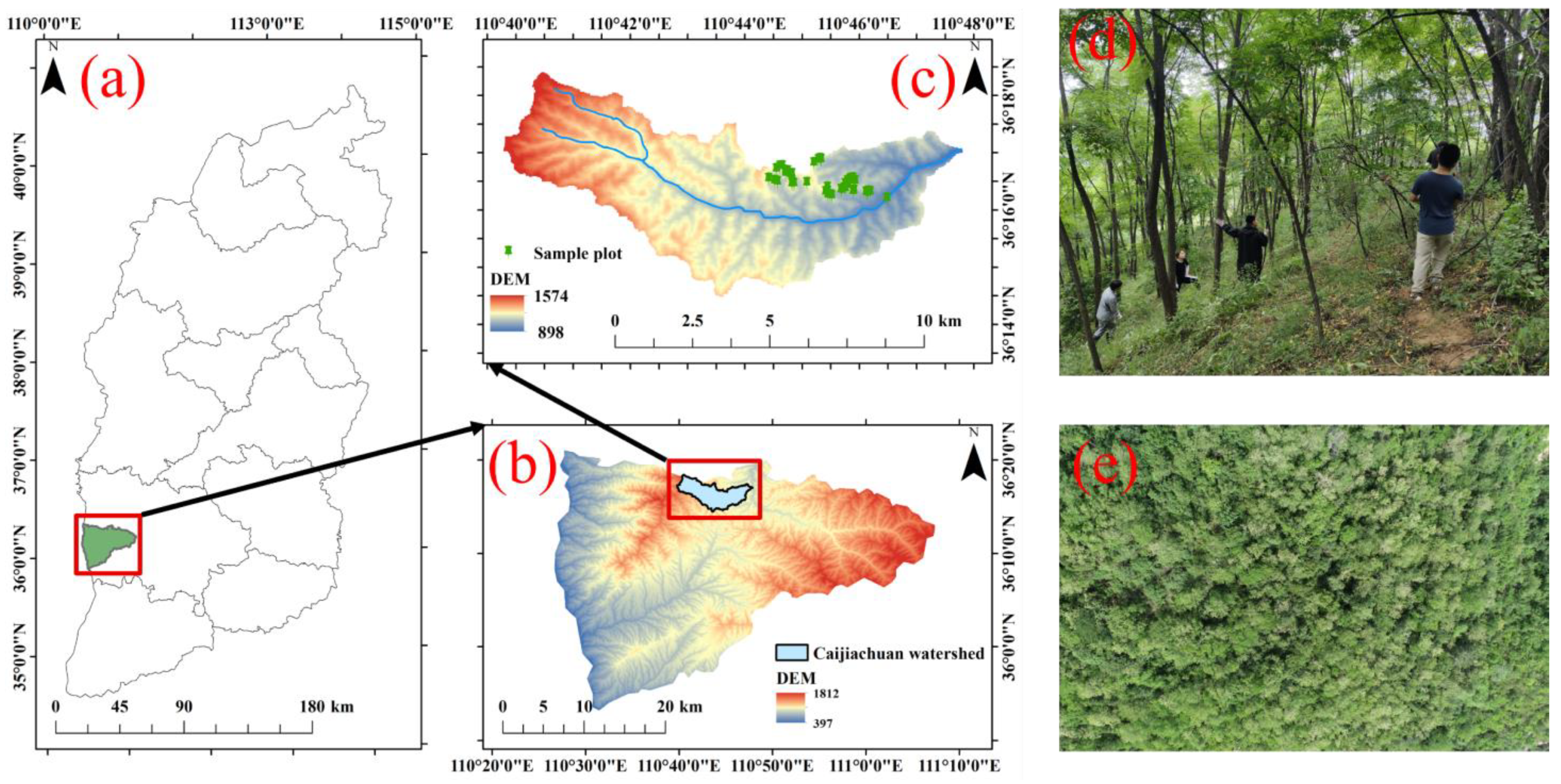
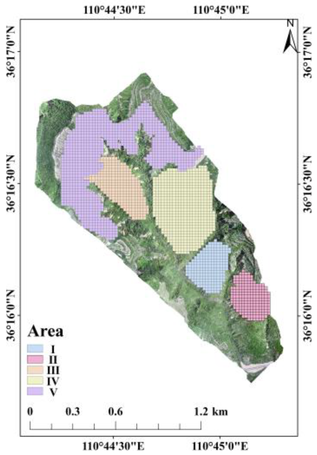
2.1. Study Area

This study was conducted at the National Forest Ecosystems Field Scientific Observatory Station in Ji County, Shanxi Province (Figure 1). The Caijiachuan watershed (36°14′27″N–36°18′23″N, 110°39′45″E–110°47′45″E) is located in the southeastern Loess Plateau, covering an area of 39.33 km² with an elevation range of 898–1574 m. The region is characterized by a loessial parent material and cinnamon soils, representing the typical hilly and gully terrain of the Loess Plateau. The watershed has a warm temperate continental climate, with an average annual temperature of 10.8 °C and an average annual precipitation of 509.0 mm, most of which occurs between July and October. The potential annual evaporation is approximately 1729 mm. The upper reaches of the Caijiachuan watershed consist of rocky and mountainous terrain dominated by natural secondary forests, while the middle and lower reaches are characterized by protective plantations, natural secondary vegetation from afforestation closures, and agricultural ecosystems. Since the 1990s, afforestation efforts have primarily introduced R. pseudoacacia, Platycladus orientalis, and Pinus tabuliformis as the dominant species. The understory vegetation predominantly includes Rosa xanthina, Artemisia gmelinii, and Carex lithophila [41].

2.2. Field Data Collection

After 30 years of restoration, the vegetation cover in the Caijiachuan watershed has significantly increased. To gain a comprehensive understanding of the growth dynamics of black locust and inform future management strategies, a detailed sampling survey was conducted (Figure S1).

To meet the accuracy requirements of forest resource sampling surveys, this study established 49 sample plots of R. pseudoacacia plantations, each measuring 20 m × 20 m, in the Caijiachuan watershed from May to September 2023. All plots consisted of R. pseudoacacia plantations established in 1994. Within each sample plot, individual trees were measured to record stand density, diameter at breast height (DBH), and H (Figure S2). The height of shrubs within the sample plots was also measured, revealing that all shrubs were below 5 m in height across the 49 sample plots. Consequently, R. pseudoacacia trees exceeding 5 m in H were reselected in each sample plot, and the density was recalculated. The sample plots were then categorized into five density gradients: 900–1200, 1201–1500, 1501–1800, 1801–2100, and 2101–2400 trees ha⁻¹. Filtering based on H was conducted to minimize the influence of shrubs on ITS and reduce potential errors. The coordinates of the four corners of each plot were measured using Real-Time Kinematic Global Navigation Satellite System (RTK-GNSS) technology, and their positions were recorded [40].

2.3. R. pseudoacacia AGB Survey

This study employed an allometric growth equation to estimate AGB, enabling nondestructive AGB measurement. To estimate the AGB of Robinia pseudoacacia, a total of 63 trees with DBH ranging from 5 to 28 cm were harvested across 49 sample plots. After harvesting, the H of the selected specimens was remeasured and recorded to validate the accuracy of the initial H measurements. Each tree was then separated into stems, branches, and leaves, with all parts collected, dried, and weighed to determine the dry AGB of each component. The total AGB of each tree was subsequently calculated using the following equation [42]:

$$W_i={\displaystyle \frac{M_{fwi}-M_{dwi}}{M_{dwi}}}$$

(1)

$$B_i=M_{tfwi}\ast \left(1-W_i\right)$$

(2)

$$B_{tb}=\sum B_i$$

(3)

where $W_i$ is the moisture content of each organ sample plot, $M_{fwi}$ is the fresh weight of each organ sample plot, $M_{dwi}$ is the dry weight of each organ sample plot, $M_{tfwi}$ is the total fresh weight of each organ sample plot, $B_i$ is the AGB of each organ sample plot, and $B_{tb}$ is the total AGB of the tree.

2.4. Disk Collection, Processing, and Analysis

Prior to harvesting standard trees, the north-facing direction was marked on the stem. A 5 cm thick disk was then extracted at DBH for tree ring analysis [35].

The tree disk used for tree ring analysis was polished using 400-grit sandpaper. It was then scanned with a scanner (Epson Perfection V600 Photo J252A, SEIKO EPSON CORP, Suwa City, Japan), with a ruler placed beside it for length calibration, resolution of 300 dpi. The resulting scanned images were analyzed using the Wanshen LA-S tree ring analysis system (LA-S, Wseen, Hangzhou, China) (Figure S3). During the analysis, tree ring widths were measured in both the north–south and east–west directions. The difference in tree ring width between the two directions represents the annual growth. The average of the tree ring widths from both directions for the same year was used to calculate the diameter for that year.

Since the chest DBH obtained from tree ring analysis may differ from the sample survey DBH, and the DBH estimated from tree rings does not account for bark thickness, this study follows the method outlined by Xu et al. [35] to correct the discrepancies between the DBH measured in different years:

$${\theta }_i={\displaystyle \frac{\left(D_{ci}-D_{ti}\right)}{N_i}}$$

(4)

where θ_i is the corrected value (cm) for each tree ring width of the ith tree, $D_{ci}$ is the DBH of the ith tree measured using a diameter tape (cm), $D_{ti}$ is the DBH (with bark thickness) calculated from the cumulative tree diameter of the $i$th tree, $N_i$ is the tree age (year) of the $i$th tree.

In this study, it is assumed that the θ_i value of each standard tree remains constant across different years. Therefore, the formula for calculating the corrected DBH of each standard tree across different years is as follows:

$$D_{cik}=D_{ik}+N_{ik}\ast {\theta }_i$$

(5)

where $D_{cik}$ represents the corrected DBH value of the $k$th age gradation of the $i$th tree, $D_{ik}$ denotes the DBH (without bark thickness) calculated from the cumulative tree diameter (m) for the $k$th age gradation of the $i$th tree, $N_{ik}$ refers to the $k$th age of the $i$th tree.

2.5. Individual Tree AGB Model and H-DBH Model Construction

To ensure accurate AGB estimation at the sample plot scale, we need to establish an H-DBH, as well as an AGB model that includes both H and DBH [43]. The H-DBH is as follows:

$$H=a\ast D^b$$

(6)

where $H$ is the tree height (m), $D$ is the DBH (cm), and $a, b$ are the regression equation parameters.

Currently, commonly used allometric growth models are typically based on indicators such as H and DBH. In this study, seven different types of allometric growth models are presented, and one optimal model is selected as the individual tree AGB model for subsequent analysis (

Table 1. The list of the AGB_IT model allometric growth equations used in this study.

Number	Equation Form	Parameters	Variate
1	${AGB}_{IT}=a{D}^b$	$a, b$	$D$$, H$
2	${AGB}_{IT}=a{H}^b$	$a, b$	$H$
3	${AGB}_{IT}=a{\left(D^{2}H\right)}^b$	$a, b$	$D$$, H$
4	${AGB}_{IT}=a{D}^b{H}^c$	$a, b, c$	$D$$, H$
5	${AGB}_{IT}=aD+b$	$a, b$	$D$
6	${AGB}_{IT}=aH+b$	$a, b$	$H$
7	${AGB}_{IT}=aD+bH+c$	$a, b, c$	$D$$, H$

Note: ${AGB}_{IT}$ is the individual tree AGB of R. pseudoacacia (kg); $H$ is the tree height (m); $D$ is the diameter at breast height (cm); $a,b,c$ are the regression equation parameters.

).

In this study, the fitting and prediction accuracy of the AGB models were evaluated by calculating the coefficient of determination ($R²$), root mean square error ($RMSE$), relative root mean square error ($\%RMSE$), as well as the absolute mean difference ($MD$) and relative mean difference ($\%MD$) between estimated and observed AGB. The relevant formulas are as follows:

$$R^2=1-{\displaystyle \frac{\left(n-1\right){\sum }_{i=1}^n{\left(B_i-\widehat{B_i}\right)}^2}{\left(n-1\right){\sum }_{i=1}^n{\left(B_i-\overline{B}\right)}^2}}$$

(7)

$$RMSE=\sqrt{{\displaystyle \frac{\sum _1^n{\left(\widehat{B_i}-B_i\right)}^2}{n}}}$$

(8)

$$\%RMSE={\displaystyle \frac{RMSE}{\overline{B}}}\times 100$$

(9)

$$MD={\displaystyle \frac{\sum _{i=1}^n\left(\widehat{B_i}-B_i\right)}{n}}$$

(10)

$$\%MD={\displaystyle \frac{MD}{\overline{B}}}\times 100$$

(11)

where $B_i$ is the observed AGB (kg); $\widehat{B_i}$ is the estimated AGB (kg); $\overline{B}$ is the sample plot mean observed AGB (kg); $n$ is the observed AGB (kg).

2.6. Sample Plot AGB of R. pseudoacacia Model Construction

To ensure accurate AGB estimation at the watershed scale, this study required the development of an AGB model based on sample plot tree density (N) and average tree height (AH). To achieve this, we reviewed seven different allometric growth models (

Table 2. The list of the AGB_SP model allometric growth equations used in this study.

Number	Equation Form	Parameters	Variate
1	${AGB}_{SP}=a{N}^b$	$a, b$	$D$$, H$
2	${AGB}_{SP}=a{\left(AH\right)}^b$	$a, b$	$H$
3	${AGB}_{SP}=a{\left(N^{2}AH\right)}^b$	$a, b$	$D$$, H$
4	${AGB}_{SP}=a{N}^b{\left(AH\right)}^c$	$a, b, c$	$D$$, H$
5	${AGB}_{SP}=aN+b$	$a, b$	$D$
6	${AGB}_{SP}=aAH+b$	$a, b$	$H$
7	${AGB}_{SP}=aN+bAH+c$	$a, b, c$	$D$$, H$

Note: ${AGB}_{SP}$ is the sample plot AGB of R. pseudoacacia (kg); $AH$ is the average tree height in the sample plot (m); $N$ is the number of R. pseudoacacia in the sample plot (tree); $a,b,c$ are the regression equation parameters.

) and selected the most optimal model for AGB estimation.

2.7. Carbon Storages Calculation

Vegetation carbon storages are calculated by multiplying vegetation AGB by the carbon content of the vegetation. The carbon content data are derived from the Shanxi Provincial Forest Resource Inventory, with a carbon content rate of 0.5 [39].

$$C=AGB\ast 0.5$$

(12)

where $C$ is the carbon storage (Mg ha⁻¹); $AGB$ is the AGB of R. pseudoacacia (Mg ha⁻¹); $0.5$ is the carbon rate of R. pseudoacacia.

2.8. Data Acquisition and Preprocessing

2.8.1. Data Acquisition

Data collection for this study was conducted from May to June 2023 using a DJI M300RTK drone equipped with the Zen L1 LiDAR. The lidar system (gAirHawk GS-130X, Wuhan Geosun Navigation Technology, Wuhan, China) was mounted on a UAV (Matrice 300, DJI, Shenzhen, China). The flight speed was 10 m/s, the flight altitude was 80 m, and the flight mode was terrain-following. The LiDAR had an overlap rate of 80%, and the average point cloud density was 147 points/m² (Figure S4).

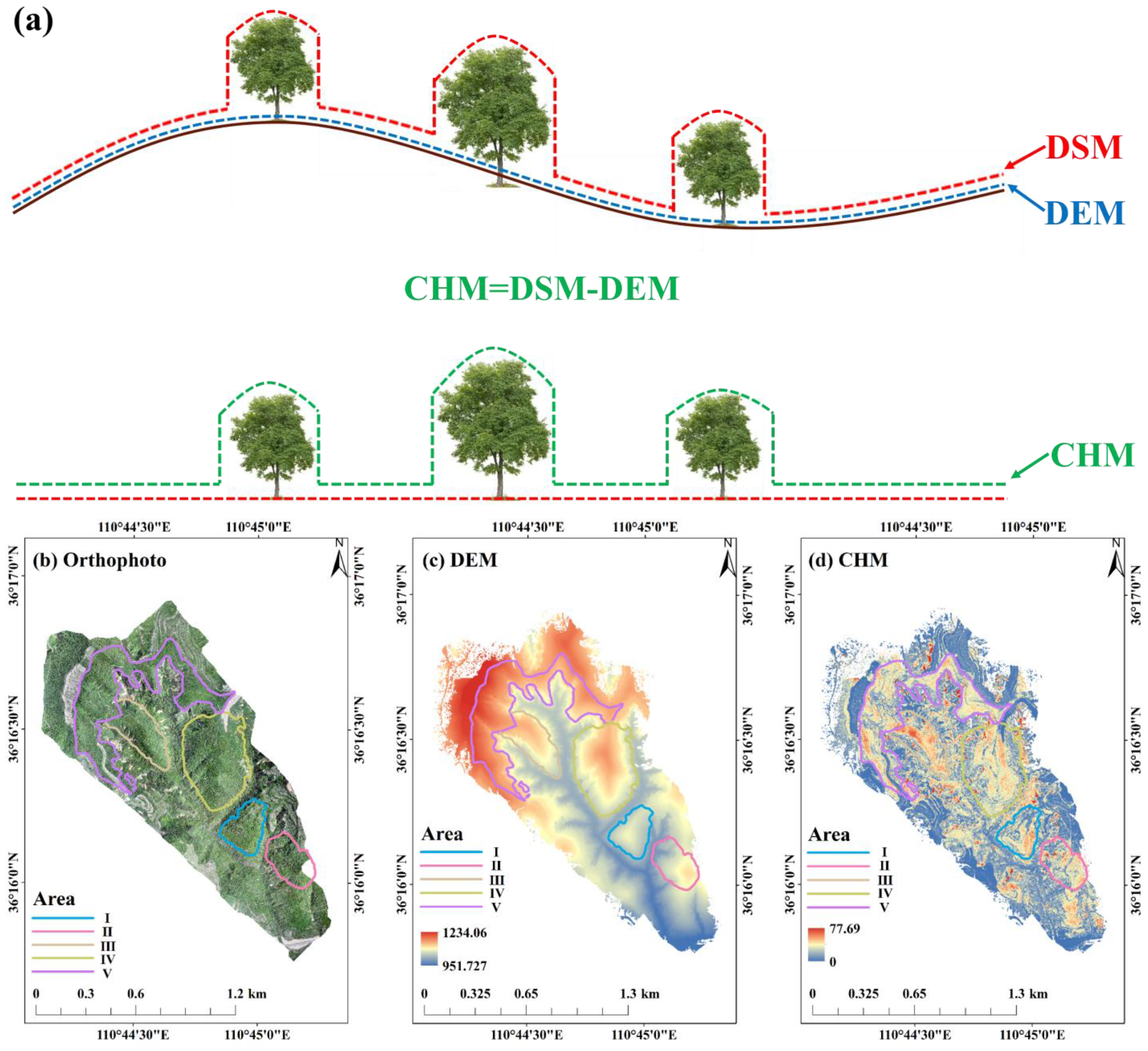
2.8.2. Data Preprocessing

After data collection, the DJI Maps software (v3.6, DJI, Shenzhen, China) was used for data stitching, resulting in a digital orthophoto map (DOM) of the study area with a spatial resolution of 1 m (Figure 2b) [44]. Using visual interpretation, five primary locations of the artificial R. pseudoacacia forests within the watershed were selected for data extraction. The data were then processed using LiDAR 360 software (v5.2, GreenValley International, Beijing, China), and ground and surface points were classified using the Improved Progressive TIN Densification [45]. Ordinary Kriging interpolation was applied to generate the digital surface model (DSM) and the digital elevation model (DEM) (Figure 2c). By subtracting the DEM from the DSM, the CHM of the study area was obtained (Figure 2a,d), with a spatial resolution of 0.5 m [17].

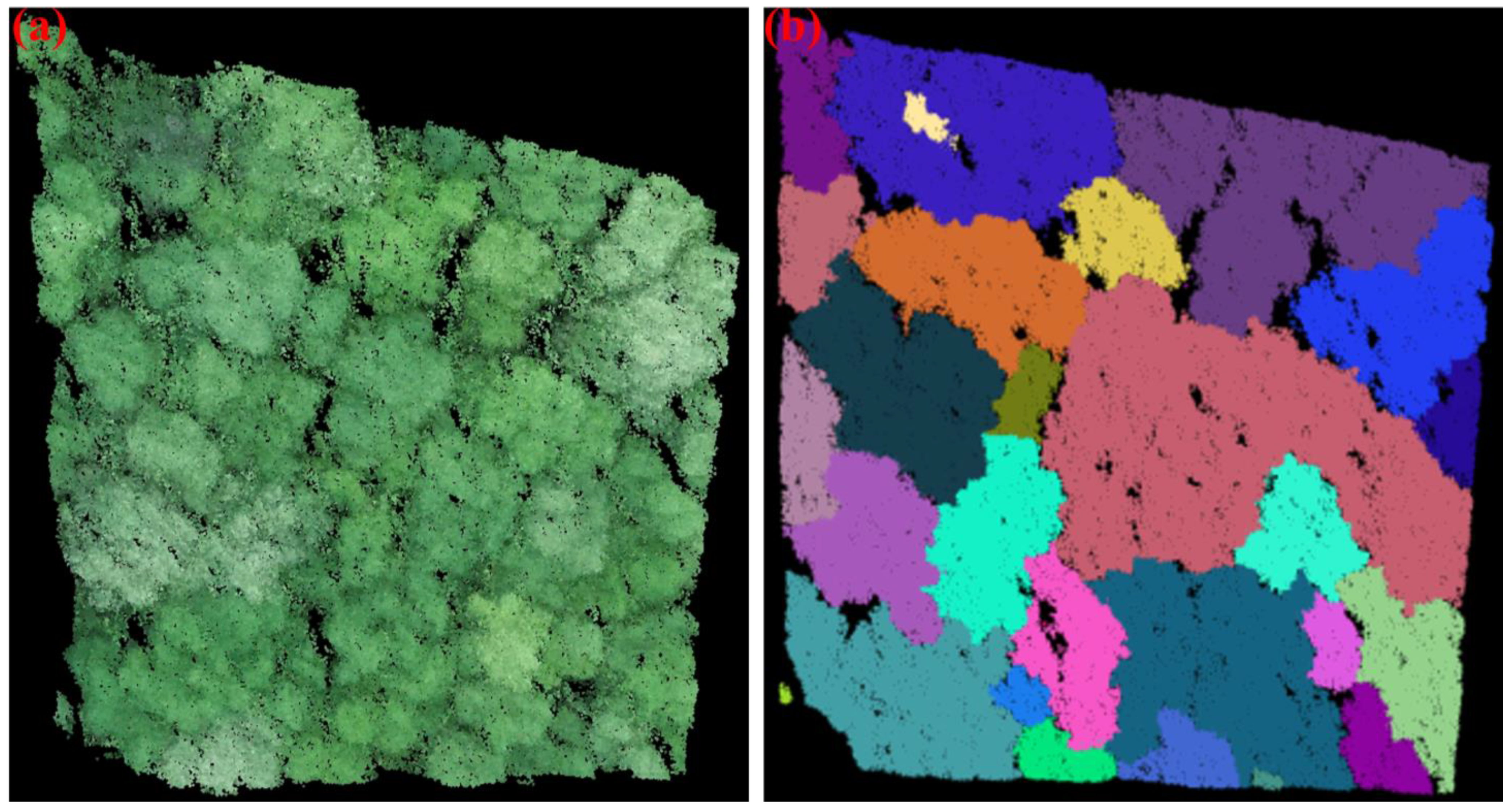
2.8.3. ITS and Forest Stand Parameter Extraction

The ITS process was primarily carried out using the point cloud toolbox in MATLAB R2023b (R2023b, MathWorks, Natick, MA, USA) (Figure 3). First, individual tree locations were detected to identify the apex of the tree crown. The extracted tree apex points were then used as seed points for crown segmentation. During the identification of tree tops, a local maxima algorithm was employed. This algorithm scanned raster data using a sliding window approach, iteratively assessing whether the center pixel of the window represented a local maximum. If identified as a maximum, the corresponding pixel was designated as the tree apex. Subsequently, a watershed segmentation algorithm was employed to accurately segment each individual tree crown using an optimal segmentation window, thus extracting H data [44].

2.8.4. Accuracy of ITS

This study evaluates the performance of the ITS method based on the CHM using three statistical parameters: tree detection rate ($r$), detection accuracy of detected trees ($p$), and overall accuracy ($F$). These parameters are defined as follows [32]:

$$r={\displaystyle \frac{TP}{TP+FN}}$$

(13)

$$p={\displaystyle \frac{TP}{TP+FP}}$$

(14)

$$F=2\times {\displaystyle \frac{r\times p}{r+p}}$$

(15)

where $TP$ is the number of detected trees in a sample plot; $FN$ is the number of trees omitted by ITS and $FP$ is the number of trees falsely detected in the sample plot.

2.8.5. Extraction Error of Forest Stand Parameters

The error rates of the number of trees, H, and AGB obtained using the ITS method based on the CHM were calculated by comparing the sample plot survey data (observed values) with the point cloud data extraction results (estimated values) [40]:

$$e={\displaystyle \frac{\left(\left|E-M\right|\right)}{M}}\times \%$$

(16)

where $e$ is the error rate; $E$ is the estimated values; $M$ is the observed values.

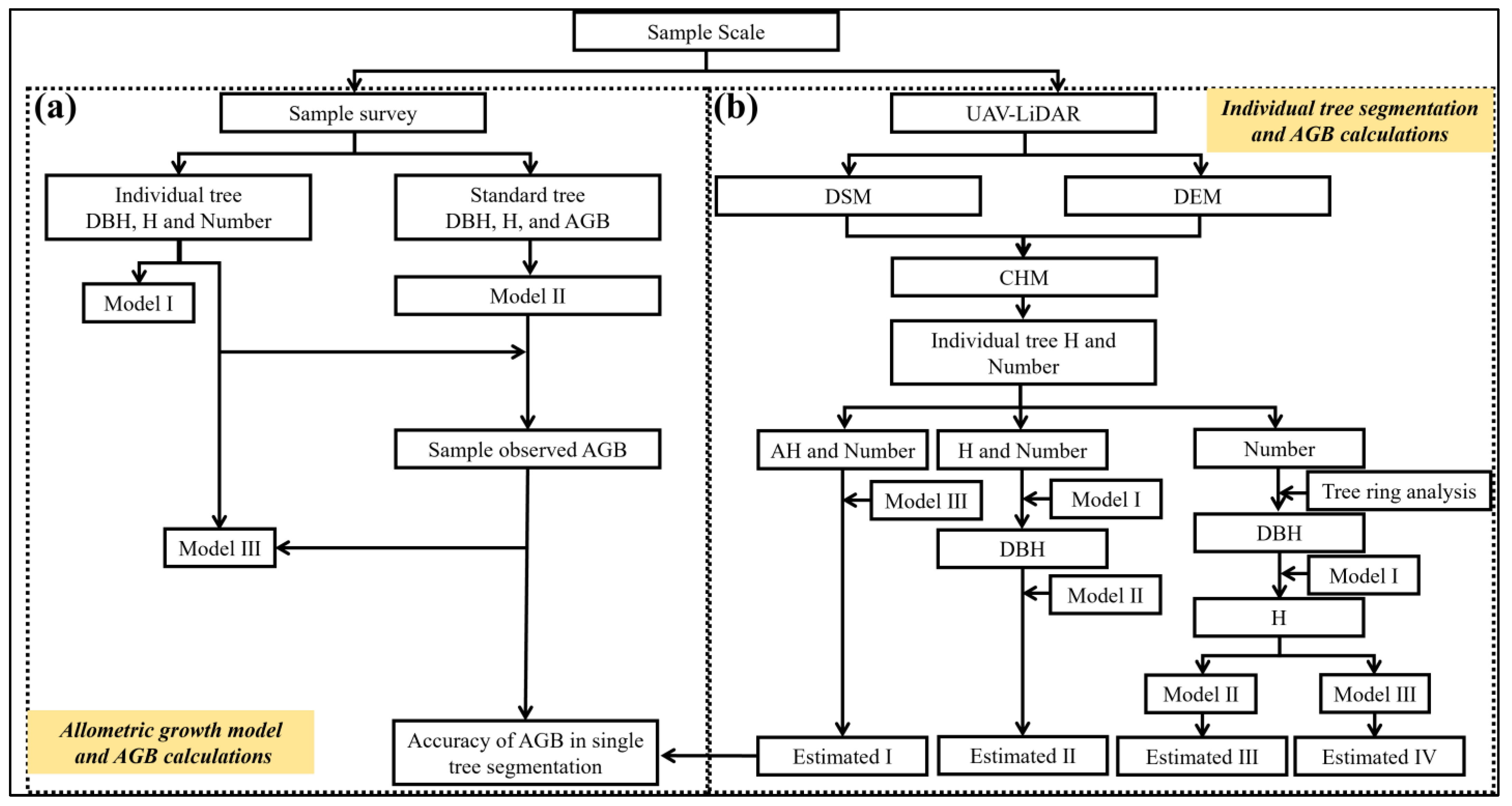
2.8.6. Biomass Estimation Methods

In this study, the observed AGB at the sample plot scale was calculated as the sum of the individual tree AGB of R. pseudoacacia within the sample plot. The estimated sample plot scale AGB was derived from the N and H from ULS, using four different calculation methods (Figure 4):

Method 1: The N and AH were input into the AGBSP model to estimate the sample plot AGB (Estimated I).

Method 2: Based on the N from ULS, the corresponding density was determined. The H was then input into the H-DBH relationship for the respective density to obtain the corresponding DBH. The individual tree AGB was calculated using the AGB_IT model with the H and DBH values for each tree. The sum of the individual tree AGB within the sample plot was taken as the estimated sample plot AGB (Estimated II).

Method 3: Based on the N from ULS, the corresponding density was determined. The appropriate tree growth curve was selected, and the known stand age was input into the curve to obtain the DBH of the standard tree for the sample plot. The H of the standard tree was calculated using the H-DBH model. The individual tree AGB was then calculated using the AGBIT model with the DBH and H values. The product of the individual tree AGB and the N was taken as the estimated sample plot AGB (Estimated III).

Method 4: The H obtained from Method III was used as the AH for the sample plot. This AH and the N were input into the AGB_SP model to estimate the sample plot AGB (Estimated IV).

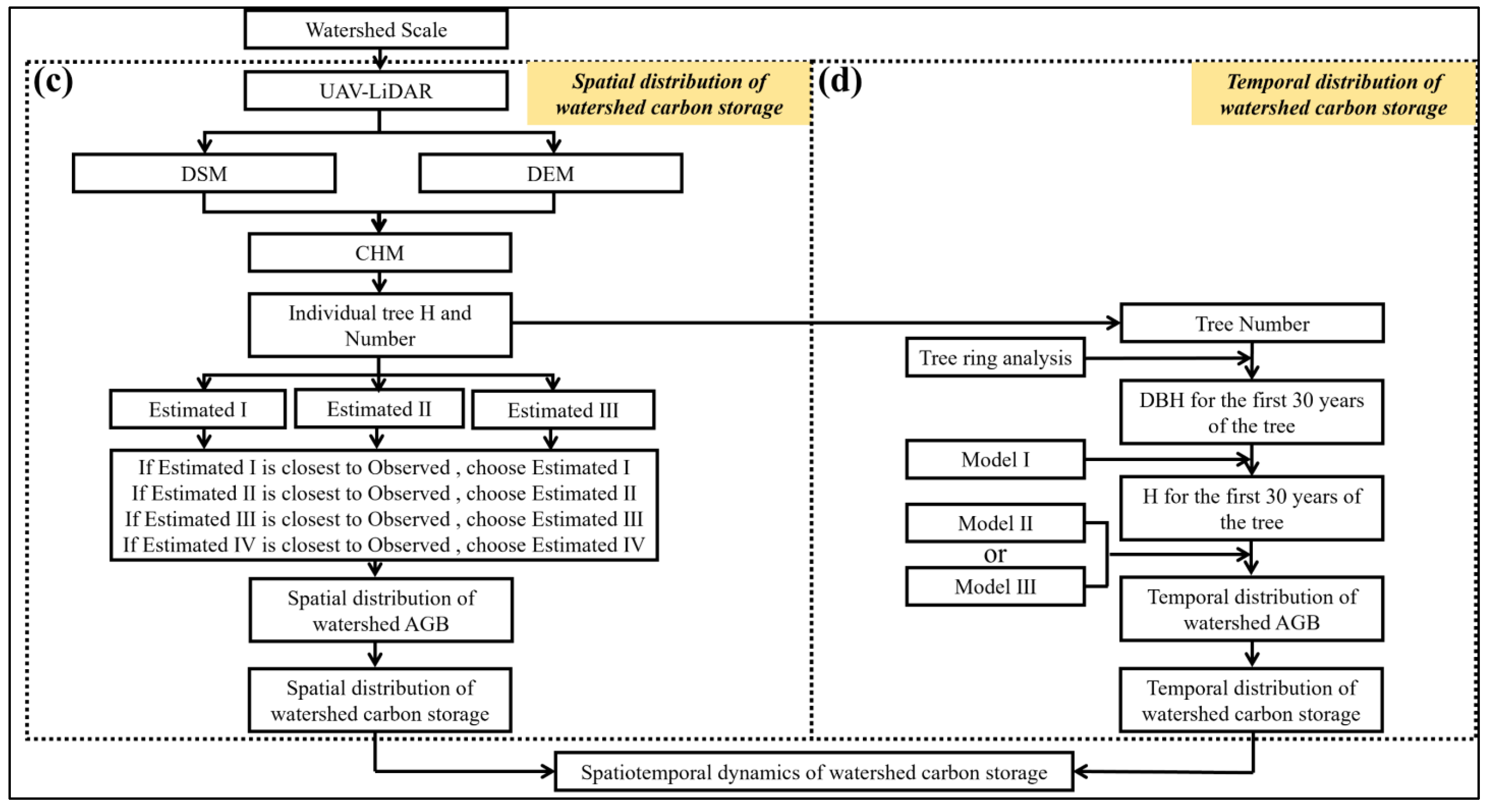
2.9. Mapping the Spatiotemporal Distribution of Carbon Sink Capacity at the Watershed Scale

In this study, remote sensing imagery of the entire watershed was obtained, and the R. pseudoacacia forest areas were delineated through visual interpretation and sample plot surveys, with five specific regions selected. These five regions were then divided into continuous 20 m × 20 m grid cells, and for grid cells with areas smaller than 20 m × 20 m at the boundaries, actual area measurements were conducted to ensure accurate density calculations (Figure 5). The grid data were processed using an ITS method based on the CHM, and after data filtering, R. pseudoacacia density and individual tree H were obtained for each grid cell. These data were used for AGB estimation. To ensure the accuracy of AGB estimates, third prediction methods closest to the sample plot observed AGB values were selected and multiplied by the corresponding carbon storage ratio to calculate the associated carbon density. The carbon storage of each grid cell was then imported into ArcGIS 10.2 (10.2, Esri, Redlands, CA, USA) to generate a spatial distribution map of the current carbon storage at the watershed scale. Furthermore, the tree ring growth curve was combined with the R. pseudoacacia density in each grid cell to calculate the temporal trend of R. pseudoacacia AGB across the watershed as it changes with forest age. The temporal and spatial distribution map of carbon storage in the watershed was then generated, integrating vegetation carbon content.

3. Results

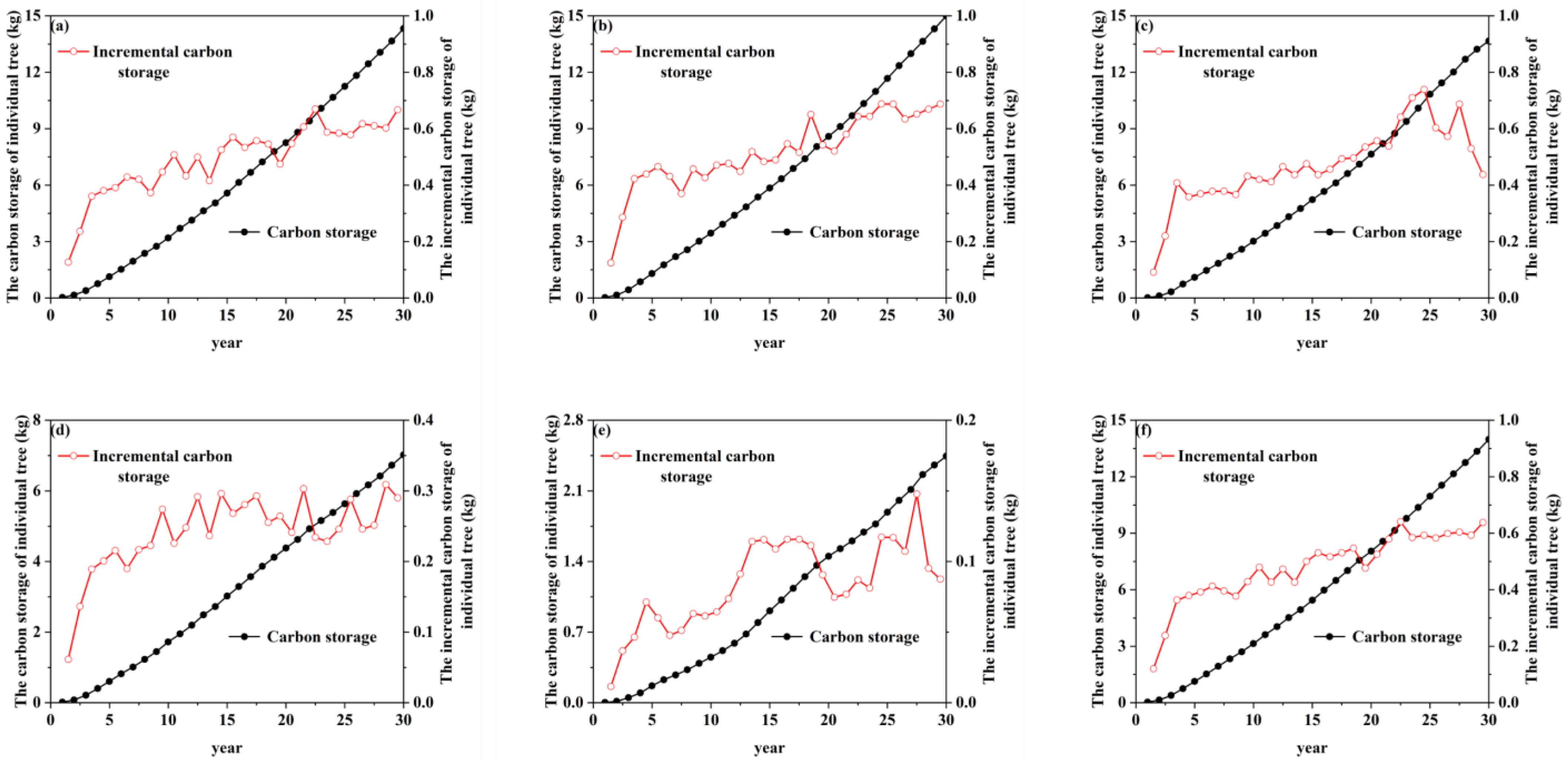
3.1. Growth Process and AGB Estimation of R. pseudoacacia

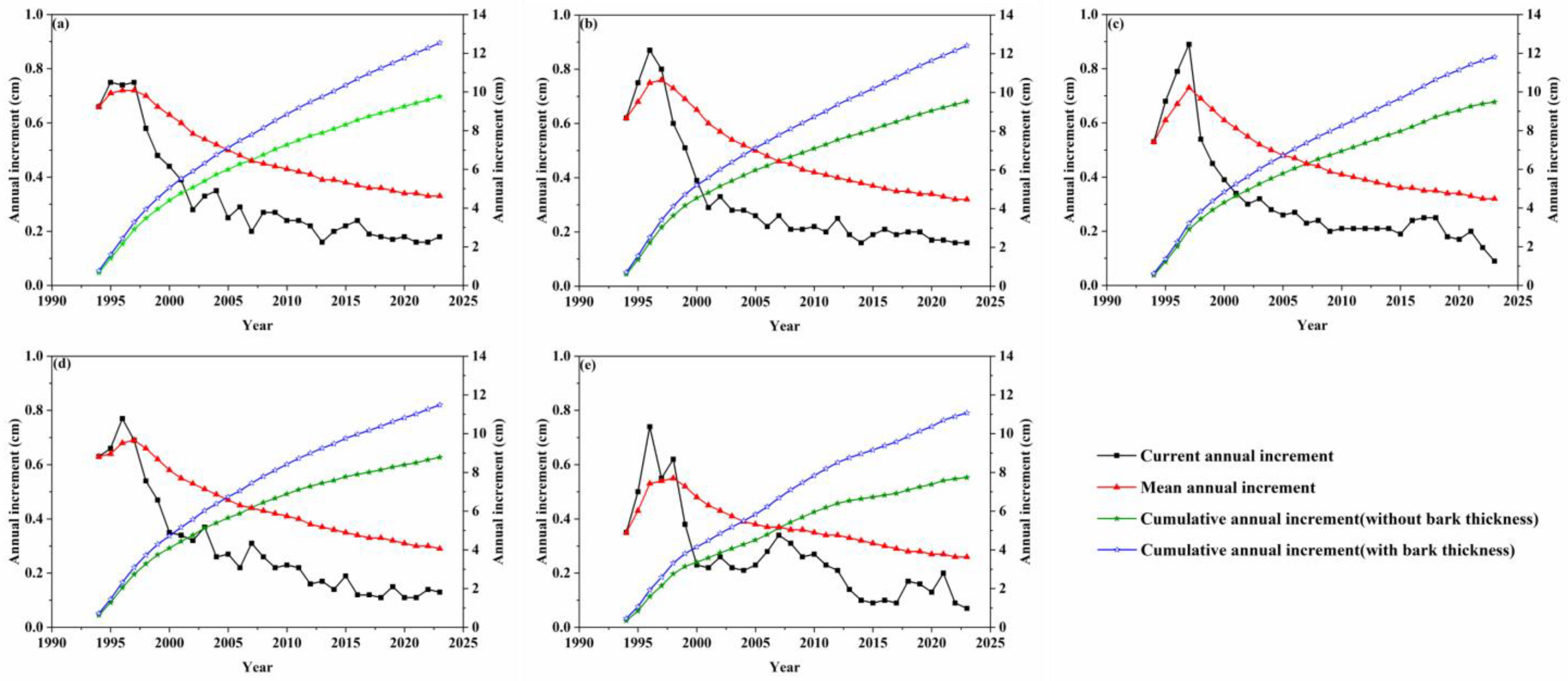
3.1.1. R. pseudoacacia Growth Curve

Analysis of the radial growth process of R. pseudoacacia across different densities revealed distinct growth patterns. During the early stages of stand development, specifically when the stand age was less than 5 years, R. pseudoacacia exhibited a rapid growth phase, with annual increments significantly exceeding the average growth rate. However, as the stand age surpassed 5 years, the growth rate of R. pseudoacacia gradually decelerated. Notably, this deceleration became more pronounced with increasing density (Figure 6).

3.1.2. H-DBH Model

The relationship between H-DBH of R. pseudoacacia was modeled, and the results showed that, under various density conditions, both H and DBH follow the power law model H = aD^b. The coefficient of determination (R²) for all cases exceeds 0.51 (

Table 3. H-DBH fitting relationship under different density conditions.

Density (Trees ha−1)	Model	R2	n
900–1200	H = 2.889D0.5043	0.5819	402
1201–1500	H = 2.741D0.5274	0.6306	745
1501–1800	H = 2.505D0.5501	0.6307	796
1801–2100	H = 2.682D0.4970	0.5107	502
2101–2400	H = 2.462D0.5337	0.6310	94

Note: n is the number of R. pseudoacacia (tree).

).

3.1.3. Individual Tree AGB of R. pseudoacacia Model Construction

Seven models were developed with DBH and H as explanatory variables, and AGB as the response variable (

Table 4. Individual tree AGB model of R. pseudoacacia.

Equation Form	Coefficients			R2	RMSE (kg)	RMSE (%)	MD (kg)	MD (%)	n
	a	b	c
${AGB}_{IT}=a{D}^b$	0.2257	2.144	—	0.9520	13.35	23.54	0.02	0.03	63
${AGB}_{IT}=a{H}^b$	0.0031	3.866	—	0.8406	24.33	42.91	−0.05	−0.09	63
${AGB}_{IT}=a{\left(D^{2}H\right)}^b$	0.0693	0.8714	—	0.9689	10.76	18.96	−0.003	−0.006	63
${AGB}_{IT}=a{D}^b{H}^c$	0.0477	1.608	1.154	0.9694	10.57	18.64	−0.01	−0.02	63
${AGB}_{IT}=aD+b$	11.18	−80.8	—	0.9210	17.14	30.21	0.002	0.003	63
${AGB}_{IT}=aH+b$	16.18	−131.9	—	0.7155	32.51	57.33	0.001	0.002	63
${AGB}_{IT}=aD+bH+c$	10.85	0.6095	−83.9	0.9199	17.11	30.17	0.001	0.001	63

Note: ${AGB}_{IT}$ is the individual tree AGB of R. pseudoacacia (kg); $H$ is the tree height (m); $D$ is the diameter at breast height (cm); $a,b,c$ are the regression equation parameters, n is the number of R. pseudoacacia (tree).

). Model selection was based on the R², root mean square error (RMSE), and the simplicity of the equation form. After comparing the R² and RMSE of the seven models, the model of the form ${AGB}_{IT}=a{D}^b{H}^c$ was found to have the highest R² (R² = 0.9694) and the lowest RMSE (RMSE = 10.57). Additionally, its absolute mean deviation (MD) was less than 1 kg (<1%), indicating strong robustness. A Wilcoxon rank sum test revealed no significant difference between the estimated and observed values of individual tree AGB (p-value = 0.909).

3.1.4. Sample Plot Observed AGB of R. pseudoacacia Observed

The influence of R. pseudoacacia density on AGB density at the stand level and individual tree AGB is illustrated in Figure 7. At the sample plot scale, AGB density significantly increased with increasing density (p < 0.05) (Figure 7a), whereas individual tree scale AGB decreased significantly as density increased (p < 0.05) (Figure 7b).

3.1.5. Sample Plot AGB of R. pseudoacacia Model

Seven different models were developed using the number of R. pseudoacacia N and AH within the stand as explanatory variables, and the total AGB of the R. pseudoacacia as the response variable (

Table 5. Sample plot AGB model of R. pseudoacacia.

Equation Form	Coefficients			R2	RMSE (kg)	RMSE (%)	MD (kg)	MD (%)	N
	a	b	c
${AGB}_{SP}=a{N}^b$	183.9	0.6333	—	0.1928	828.29	35.86	0.1152	0.0050	49
${AGB}_{SP}=a{AH}^b$	15.81	2.015	—	0.5131	643.27	27.85	−0.0538	−0.0023	49
${AGB}_{SP}=a{\left(N^{2}AH\right)}^b$	16.76	0.4797	—	0.3963	757.91	32.82	5.5429	0.2400	49
${AGB}_{SP}=a{N}^b{AH}^c$	0.1067	0.988	2.437	0.9099	273.78	11.85	0.0056	0.0002	49
${AGB}_{SP}=aN+b$	28.18	752.9	—	0.1773	836.16	36.20	0.0030	0.0001	49
${AGB}_{SP}=aAH+b$	412.5	−2538	—	0.5090	645.96	27.97	−0.0024	−0.0001	49
${AGB}_{SP}=aN+bAH+c$	38.41	478.4	−5434	0.8616	339.33	14.69	0.0063	0.0003	49

Note: ${AGB}_{SP}$ is the sample plot AGB of R. pseudoacacia (kg); $AH$ is the average tree height of Robinia pseudoacacia in the sample plots (m); $N$ is the number of R. pseudoacacia in the sample plots (tree); $a,b,c$ are the regression equation parameters; the best results for each indicator are shown in bold.

). The optimal model was selected based on the R², RMSE, and the simplicity of the equation. A comparison of the R² and RMSE values for the seven models revealed that the equation ${AGB}_{SS}=a{D}^b{AH}^c$ produced the best fit, with an R² of 0.9099 and an RMSE of 273.78. Additionally, the MD was less than 1 kg (<1%), indicating strong model stability.

3.2. The Effect of Point Cloud Data Segmentation Window Size on ITS

3.2.1. ITS Accuracy

In 31 R. pseudoacacia sample plots, the ITS method based on the CHM exhibited variations in performance across different window sizes. The r-value reached its maximum at a window size of 0.035 m × 0.035 m, with an average of 70.99%. The highest p-value occurred at a window size of 0.080 m × 0.080 m, with an average of 98.16%. The F-value was highest at a window size of 0.060 m × 0.060 m, with an average of 79.58% (

Table 6. Accuracy assessment for the ITS method based on the CHM in different window sizes.

Segmentation Windows Size	Number of Trees	Number of Segmented Trees	TP	FN	FP	r /(%)	p /(%)	F /(%)
0.035 m × 0.035 m	1623	1895	1123	500	772	70.99	66.24	64.39
0.040 m × 0.040 m	1623	1392	1093	530	299	69.56	80.84	72.09
0.045 m × 0.045 m	1623	1246	1096	527	150	69.50	88.23	75.84
0.050 m × 0.050 m	1623	1199	1093	530	106	69.37	91.50	77.25
0.055 m × 0.055 m	1623	1166	1097	526	69	69.50	94.42	78.46
0.060 m × 0.060 m	1623	1151	1107	516	44	69.84	96.10	79.52
0.065 m × 0.065 m	1623	1120	1084	539	36	68.58	96.78	79.28
0.070 m × 0.070 m	1623	1108	1078	545	30	68.41	97.41	78.93
0.075 m × 0.075 m	1623	1098	1078	545	20	68.04	98.08	78.88
0.080 m × 0.080 m	1623	1092	1071	552	21	67.56	98.16	78.67

Note: The best results for each indicator are shown in bold.

).

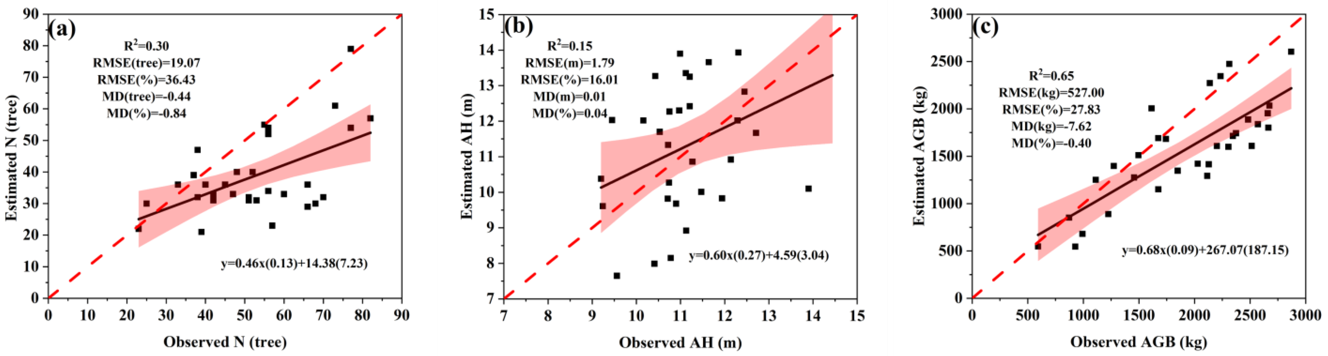
3.2.2. Error of N, AH and AGB

Table 7. Results and error rates of N and AH segmentation under 10 window sizes.

Segmentation Windows Size	N/tree	AH/m	N Error/%	AH Error/%
0.035 m × 0.035 m	1895	10.18	62.04	17.51
0.040 m × 0.040 m	1392	10.98	31.32	14.73
0.045 m × 0.045 m	1246	11.33	28.15	14.17
0.050 m × 0.050 m	1199	11.50	26.95	14.40
0.055 m × 0.055 m	1166	11.69	28.21	15.25
0.060 m × 0.060 m	1151	11.74	28.37	15.06
0.065 m × 0.065 m	1120	11.81	30.09	15.50
0.070 m × 0.070 m	1108	11.85	30.58	15.63
0.075 m × 0.075 m	1098	11.89	31.37	15.50
0.080 m × 0.080 m	1092	11.90	32.02	15.24

Note: The best results for each indicator are shown in bold.

presents the evaluation results of the ITS method based on the CHM for R. pseudoacacia, using various segmentation window sizes. As the window size increases, the N of detected R. pseudoacacia decreases, while the AH increases. The error in the N of R. pseudoacacia was smallest at a window size of 0.050 m × 0.050 m, with an error of 26.95%. The error in the stand’s AH was lowest at a window size of 0.045 m × 0.045 m, with an error of 14.17%.

Figure 8 presents the distribution of estimated versus observed values for the N of R. pseudoacacia and H using the ITS method based on the CHM. The results show that, at lower densities, the method slightly underestimates the N of R. pseudoacaci, while at higher densities, it slightly overestimates the N (Figure 8a). In contrast, H estimates are slightly overestimated at lower densities and slightly underestimated at higher densities (Figure 8b).

Table 8. Results and error rates of N, AH, and AGB_SPS segmentation under 10 window sizes.

Segmentation Windows Size	Observed/kg	Estimated I Error/%	Estimated II Error/%	Estimated III Error/%	Estimated IV Error/%
0.035 m × 0.035 m	1627.23	24.55	123.33	49.72	44.31
0.040 m × 0.040 m	1543.65	22.86	98.84	30.14	36.64
0.045 m × 0.045 m	1523.09	24.31	86.26	31.39	38.73
0.050 m × 0.050 m	1526.14	24.22	82.80	31.93	37.72
0.055 m × 0.055 m	1544.14	24.37	84.74	31.22	38.85
0.060 m × 0.060 m	1546.49	24.57	86.22	31.25	39.26
0.065 m × 0.065 m	1526.70	24.54	82.88	31.16	39.53
0.070 m × 0.070 m	1525.33	24.51	83.17	30.50	40.67
0.075 m × 0.075 m	1517.08	25.02	81.84	31.37	41.12
0.080 m × 0.080 m	1515.46	25.18	81.77	30.49	41.48

Note: The best results for each indicator are shown in bold.

presents the evaluation results of various AGB estimation methods across different segmentation window sizes. The findings indicate that the first AGB estimation method achieved the lowest error rate, 22.86%, at a window size of 0.040 m × 0.040 m. The second method exhibited the smallest error rate of 81.77% at a window size of 0.080 m × 0.080 m. The third method had the lowest error rate of 30.14% at a window size of 0.040 m × 0.040 m. Similarly, the fourth method showed its smallest error rate, 36.64%, at a window size of 0.040 m × 0.040 m. Based on the comparison of error rates between estimated and observed AGB values, the first AGB estimation method demonstrated the lowest error rate and was thus selected as the optimal method for AGB estimation at the watershed scale.

Figure 8 presents the distribution of estimated versus observed AGB values for different prediction methods (Figure 8c). The results show that the AGB estimates are slightly overestimated at lower densities and slightly underestimated at higher densities.

3.3. Spatial Distribution Characteristics of Stand Parameters at the Watershed Scale

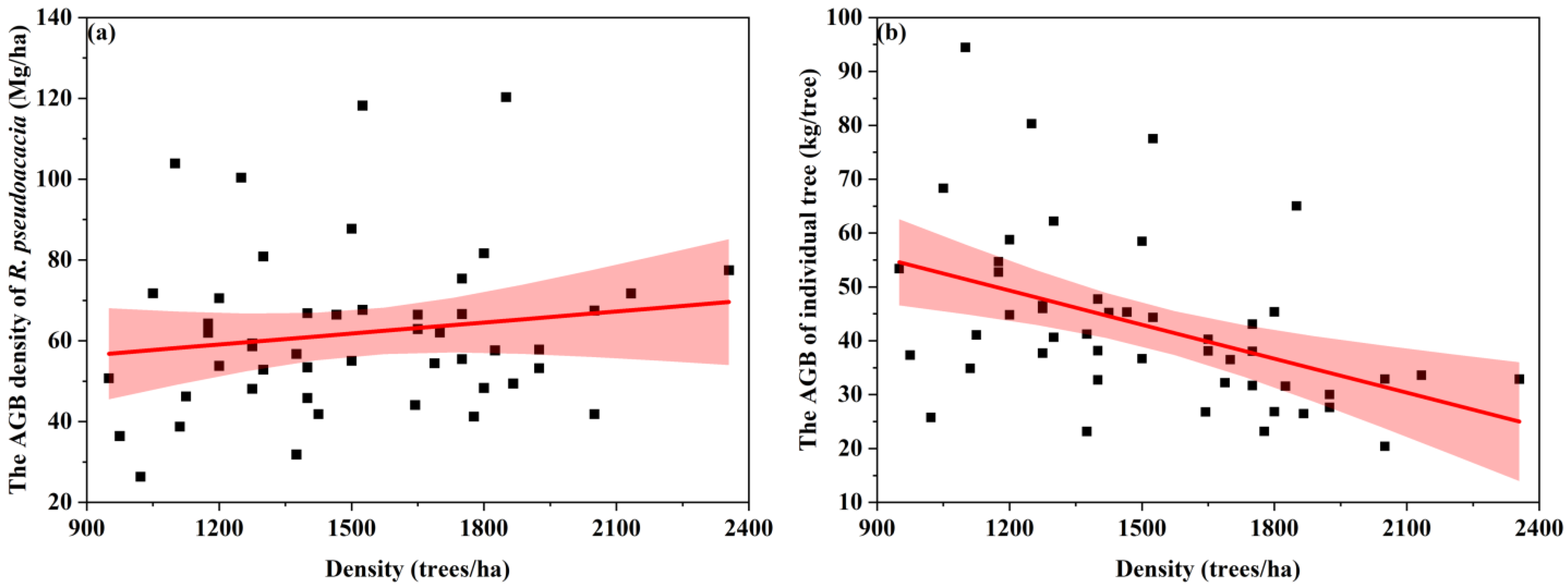
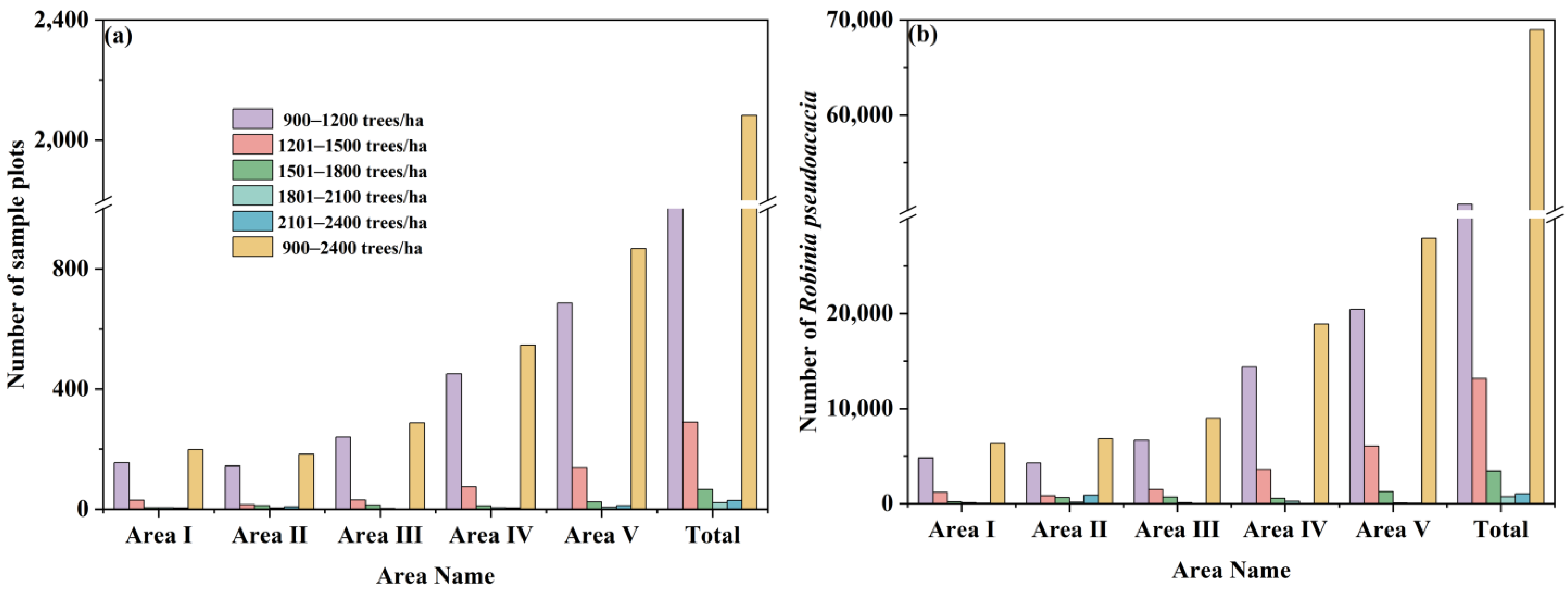
3.3.1. R. pseudoacacia Density at the Watershed Scale

The segmentation window size was set to 0.050 m × 0.050 m, and individual tree extraction was conducted across five regions. Subsequently, spatial density distribution maps for these regions were generated (Figure 9a).

The study found that a total of 2083 spatial grids, each measuring 400 m², were extracted from the R. pseudoacaci plantations within the watershed. These grids were categorized by density into five classes: D₁1676, D₂290, D₃366, D₄422, and D₅329 (Figure 10a), with 50,615, 13,173, 3436, 731, and 1037 R. pseudoacaci in each class (Figure 10b), respectively, resulting in a total of 68,992 trees. The majority of the area was occupied by R. pseudoacaci plantations with a density ranging from 900 to 1500 trees ha⁻¹.

3.3.2. The Average Tree Height at the Watershed

The segmentation window size was set to 0.045 m × 0.045 m, and individual tree extraction was performed on the spatial grids derived from the watershed point cloud data. The AH for each grid was calculated, and a spatial distribution map of the AH at the watershed scale was generated. The results indicated that the AH across the grids ranged from 5.15 to 22.69 m, with most grids showing AH between 6 and 10 m (Figure 11a). As density increased, the AH initially decreased before rising again (Figure 11b).

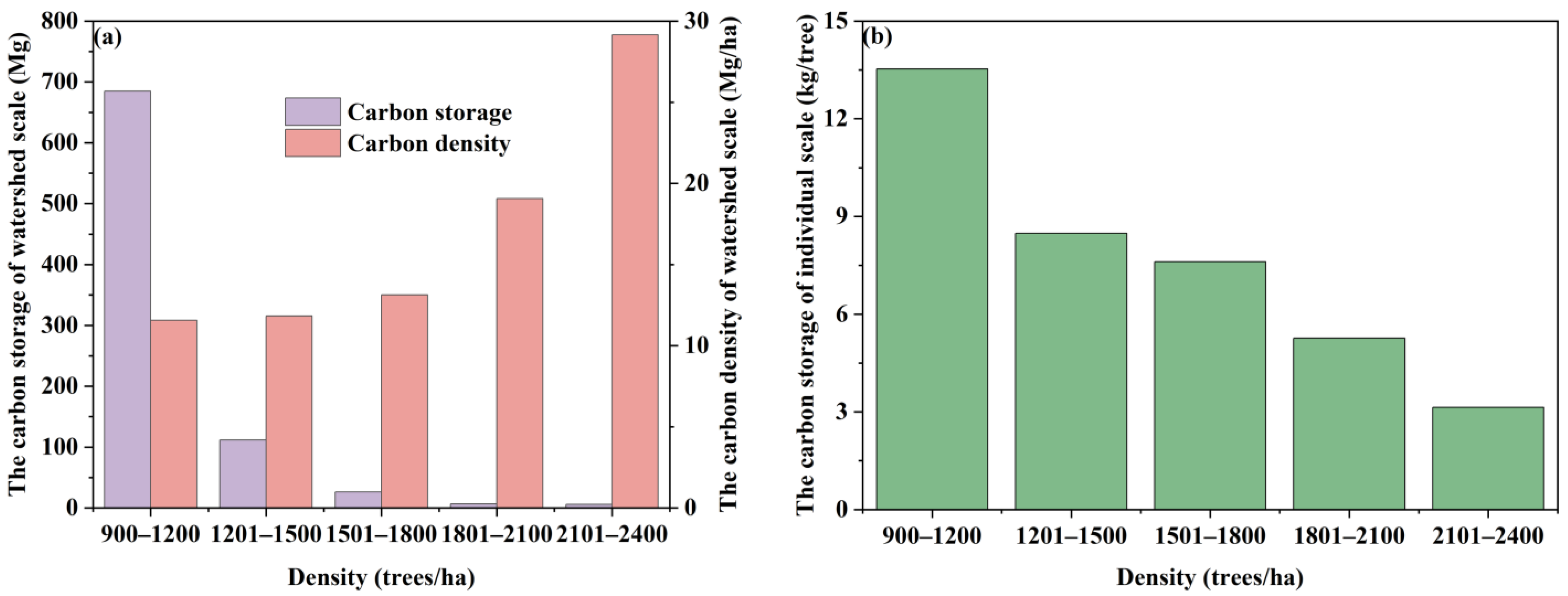
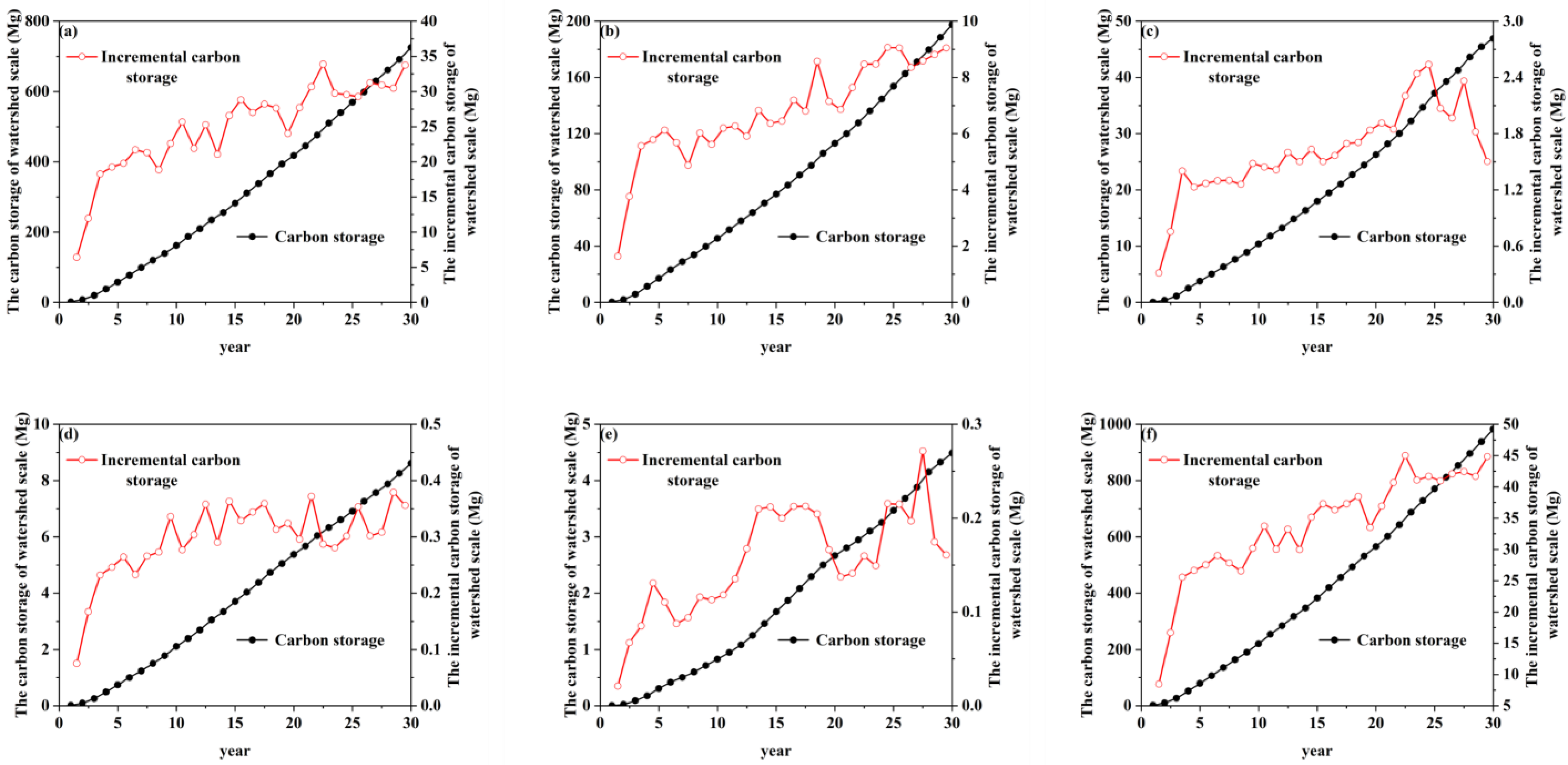
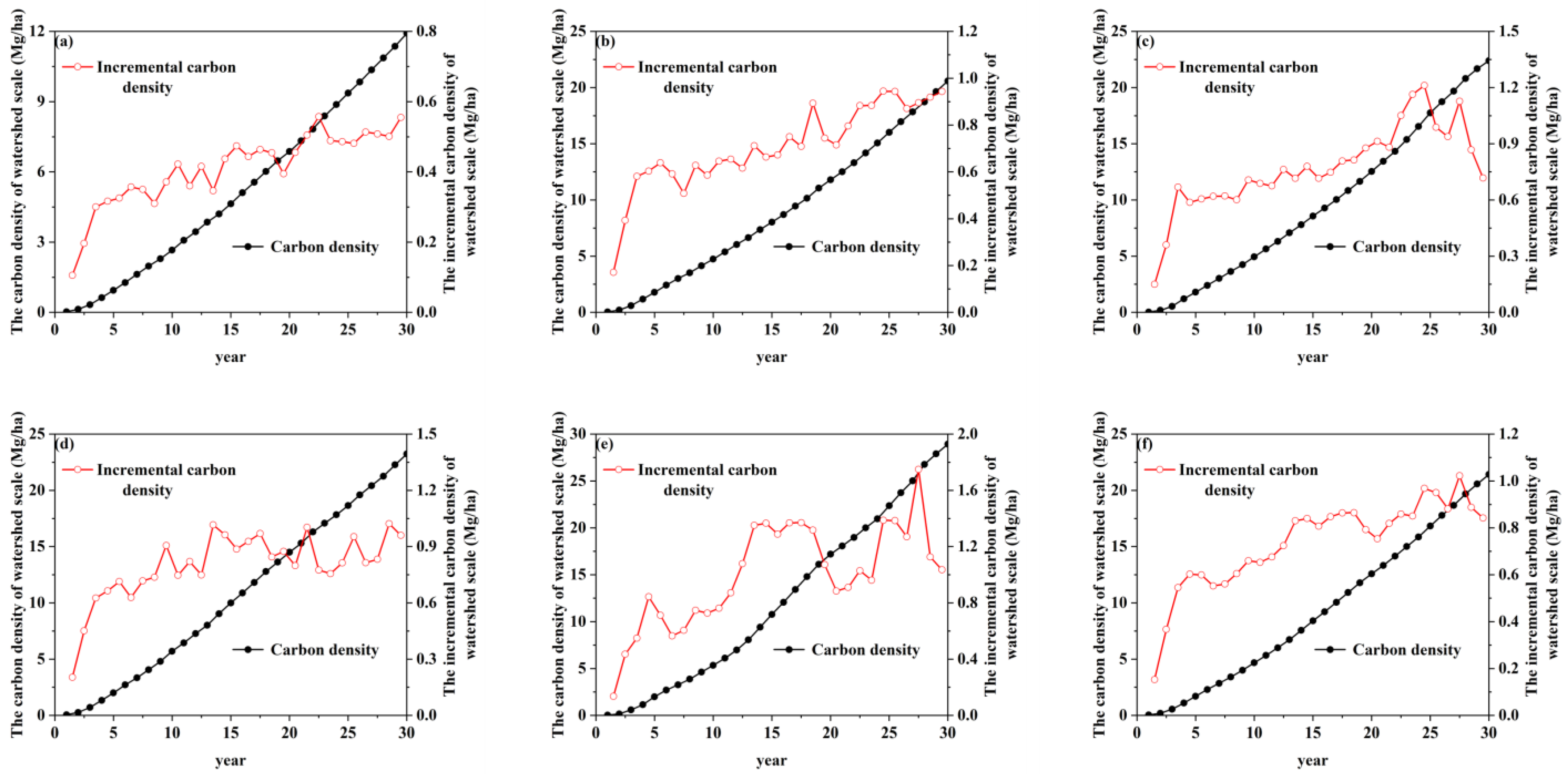
3.3.3. Estimating the Spatial Distribution of Carbon Storage and Carbon Density at the Watershed

By analyzing and calculating the N of R. pseudoacaci and the AH for each spatial grid within five regions, the AGB and AGB density for each region were estimated. These values were then used to derive the existing carbon storage and generate a spatial distribution map of carbon density at the watershed scale (Figure 9c,d).

An analysis of 2068 spatial grids revealed that the carbon storage of R. pseudoacaci at densities D₁, D₂, D₃, D₄, and D₅ were 685.03, 111.84, 26.16, 6.45, and 5.76 Mg, respectively, while the corresponding carbon densities were 11.56, 11.82, 13.13, 19.07, and 29.15 Mg ha⁻¹ (Figure 12a). The carbon storage of the R. pseudoacaci forest in the watershed was 835.24 Mg, with a carbon density of 16.95 Mg ha⁻¹. Both watershed and sample plot scale carbon densities, as well as individual tree carbon storages, exhibited similar trends: carbon density increased with density, whereas individual tree carbon storage showed the opposite trend (Figure 12a,b).

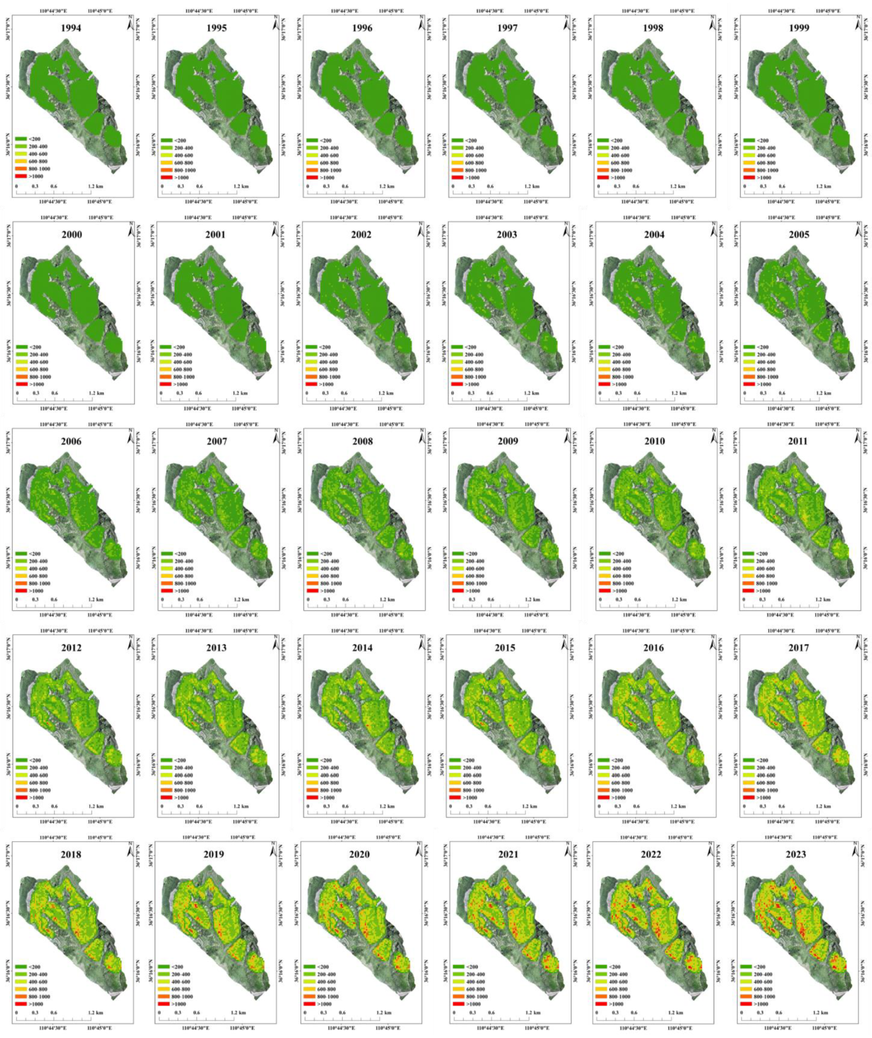
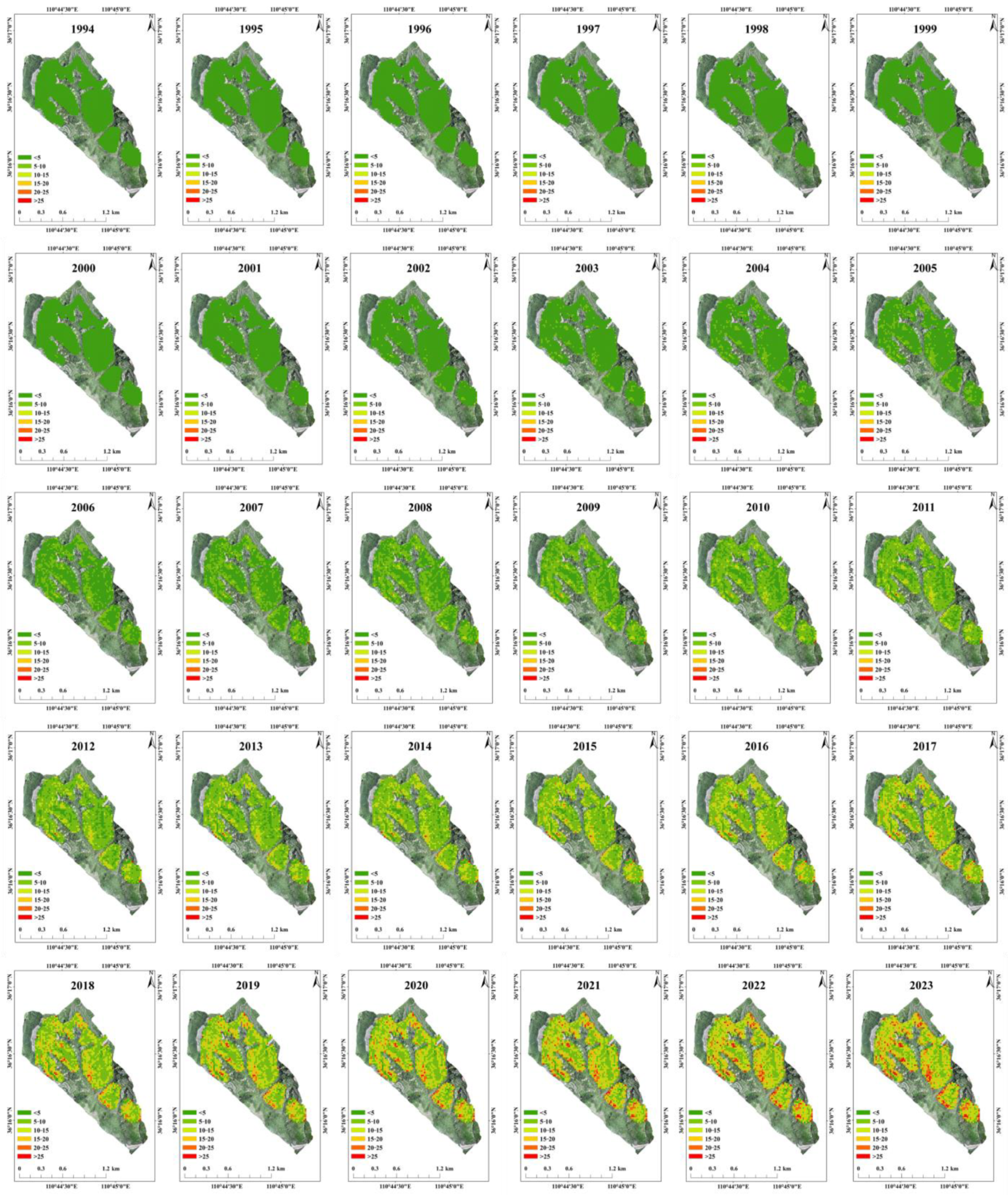
3.4. The Spatiotemporal Distribution of R. pseudoacacia Carbon Storage and Carbon Density at the Watershed Scale

The analysis reveals that Table 8, among the two methods for estimating biomass based on tree growth curves, the method with an ITS window size of 0.040 m × 0.040 m results in the smallest error. Furthermore, the error associated with the third AGB calculation method is smaller than that of the fourth method. Consequently, for estimating carbon storage and carbon density at the watershed scale over time, the third AGB estimation method is preferred.

The ITS window was set to 0.040 m × 0.040 m, and individual tree extraction was conducted for the R. pseudoacaci forest watershed to determine the density of each spatial grid. Using tree ring data, AGB and AGB density for the watershed were estimated over a 30-year period (from year 1 to year 30). Based on these estimates, the corresponding carbon storage (Figure 13) and carbon density (Figure 14) for each year were calculated.

Figure 15 presents the trends of the cumulative and current annual increment of carbon storage over a 30-year period in the Caijiachuan R. pseudoacaci forest watershed at different densities (Figure 15). Under the same density conditions, carbon storage cumulative annual increment with forest age for all five density levels, while the carbon storage current annual increment initially rises and then declines. The turning points in carbon storage’s current annual increment occur at slightly different years for each density, with the turning point shifting to later years as density increases.

Figure 16 presents the trends of the cumulative and current annual increment of carbon density over a 30-year period (Figure 16). Under consistent density conditions, carbon density cumulative annual increment follows a similar pattern to carbon density growth, and carbon density current annual increment exhibits a comparable trend. Moreover, at the same forest age, both carbon density cumulative and current annual increment increase with higher density.

Figure 17 presents the trends of cumulative and current annual increments of individual tree carbon storage over a 30-year period (Figure 17). Under consistent density conditions, as forest age increases, the patterns of cumulative annual increment of individual tree carbon storage mirror those of carbon storage and carbon density at the forest level. Similarly, the trends of the current annual increment of individual tree carbon storage with the current annual increments of carbon storage and carbon density at the forest level. At the same forest age, as density increases, both cumulative and current annual increments of individual tree carbon storage exhibit a declining trend.

4. Discussion

4.1. The Sample Plot Scale AGB of R. pseudoacacia

LiDAR technology offers significant advantages in capturing 3D forest structural information and conducting ITS. Currently, a range of algorithms, including regression trees, linear regression, and Random Forest, are utilized for estimating forest AGB from LiDAR data [22]. This study adopts ITS to estimate forest AGB, with the goal of obtaining spatial distribution information for R. pseudoacaci within the study area and estimating AGB over time by integrating tree ring data. Research has demonstrated that point cloud data obtained from LiDAR mounted on drones, combined with H data extracted through ITS, exhibits high precision [46]. However, LiDAR signals attenuate when penetrating dense canopy layers, resulting in significant errors in the extracted DBH data [47], which can negatively impact the accuracy of allometric growth models that rely on both H and DBH. To address this issue in watershed-scale AGB estimation, the study innovatively uses N and AH to construct allometric growth equations, thus avoiding the large errors in DBH data associated with ITS [48].

This study employed four methods for AGB estimation at the sample plot scale. Among these, the method utilizing N and AH (Estimated I) yielded the most accurate estimates, closely matching the sample plot observed AGB. This approach establishes a relationship between AGB, N, and AH using sample plot observed data, and directly applies the N and AH extracted from drone-based detection to estimate AGB. This method is relatively straightforward in terms of indicator selection and model computation, reducing errors in the calculation process. Additionally, the precision of N and H, derived from drone LiDAR data through ITS, is relatively high. In contrast, the other three methods rely on H-DBH models for AGB estimation, which tend to introduce larger errors. Consequently, Prediction I was selected as the reference for analysis and comparison in this study.

By comparing the ITS results at the sample plot scale with the field survey data, it was found that the number of R. pseudoacacia was underestimated in 80.65% of the sample plots, with an RMSE of 19.07 m for N. This finding contrasts with the results of previous studies. Unlike previous research that primarily focused on coniferous forests or conical tree species [49], the tree species selected in this study, R. pseudoacacia, has a relatively flat and dense canopy with overlapping crowns, making individual tree identification more challenging. Additionally, the presence of larger trees overshadowing smaller ones leads to the omission of smaller trees in the segmentation process, thereby significantly affecting the accuracy of ITS [50]. Wang et al. [51] achieved an ITS accuracy rate of over 99% for oil palm trees, which is notably higher than the results obtained in this study. The primary reason for this discrepancy is that Wang et al.’s [51] study was conducted in a plain area with low tree density and significant gaps between trees, and the oil palm tree canopies were easily identifiable, facilitating accurate ITS. In contrast, the complex terrain and higher density in this study significantly impacted the accuracy of ITS. Lin et al. [52] investigated the effects of different vegetation cover conditions on ULS and image data and found that tree identification accuracy was 0.98 when all leaves had fallen and 0.88 when some leaves had fallen, both of which are significantly higher than under full leaf cover conditions. Therefore, in future research on ITS in R. pseudoacacia plantations, ULS data can be acquired under both leaf-on and leaf-off conditions to compare differences in point cloud density at various heights and ITS accuracy.

In this study, the AH of R. pseudoacacia was overestimated in 54.84% of the sample plots, with an RMSE of 1.79 m between the estimated and observed tree heights. In contrast, Birdal et al. [53] reported an RMSE of 0.28 m for the difference between estimated and observed tree heights. The discrepancy in RMSE values may be attributed to factors such as terrain characteristics (e.g., slope, aspect, tree species, density), flight altitude, point cloud density, and data acquisition timing [54]. The accuracy of the digital elevation model (DEM) is crucial for the precise extraction of H [55]. The lower H extraction accuracy in this study compared to other research may be due to the selected plots being located in mountainous areas with significant slopes and high tree densities, which in turn led to lower DEM accuracy and consequently affected the accuracy of tree height extraction. Another possible reason for the overestimation of H in this study could be the irregular shape of R. pseudoacacia canopies. Canopy points from taller trees may have been incorrectly segmented onto adjacent smaller trees, resulting in an overestimation of the height of these smaller trees and, subsequently, an overestimation of the overall plot H [50].

The AGB RMSE in this study was 27.83%, which is higher than that reported by Costa et al. [29]. The primary reason for this difference is that the focus of this study was on deciduous broadleaf forests, where dense canopies pose significant challenges for ITS, thereby resulting in larger AGB estimation errors. Compared to studies focusing solely on R. pseudoacacia plantations, the AGB RMSE in this study is also higher than that reported by Lu et al. [32], mainly because this study was conducted in an area with more complex terrain. In contrast, previous studies were located in plains where the acquisition of DEM is more convenient and accurate, leading to higher precision in AGB estimation.

In the current context where extracting individual tree DBH is challenging, we have innovatively proposed a method based on plot AGB, N, and AH to construct an allometric growth model. This approach avoids errors associated with DBH extraction and provides a new perspective for future AGB estimation based on ULS. To estimate AGB using N and AH from a plot, it is only necessary to establish one allometric growth model. However, if one wishes to estimate AGB using DBH and H, since ULS cannot obtain DBH data, an additional H-DBH allometric growth model is required to calculate DBH, which further increases the error. Additionally, existing studies have proposed an allometric growth model based on AGB, canopy width, and H, which avoids errors associated with DBH acquisition and estimation, also providing a new method for remote sensing-based AGB estimation [44].

4.2. The Watershed Carbon Storage and Carbon Density of R. pseudoacacia

The carbon content of forest vegetation is a fundamental parameter for estimating forest carbon storage. However, obtaining accurate carbon content values under various conditions can be challenging due to practical limitations. Consequently, many researchers have adopted a uniform carbon content coefficient of 0.50 [56] or 0.45 [57] in their estimations of forest carbon storage. Wang [58], focusing on the forest ecosystem in Shanxi Province, discovered that the carbon content among different organs of R. pseudoacacia plantations exhibits minimal variability. Specifically, there were no significant differences in carbon content among organs within the same age group or across different age groups. Wang et al. [59] similarly found that carbon content variations among different organs and age groups of R. pseudoacacia were negligible. Liu et al. [60] reported that for R. pseudoacacia stands younger than 30 years, root carbon content did not significantly change with increasing stand age. Zhang et al. [61] observed no significant differences in leaf carbon content with increasing stand age. Bai et al. [62] found no significant differences in carbon content between leaves and branches. Cao et al. [63] reported no significant differences in carbon content between branches and trunks. Liu [64], investigating R. pseudoacacia in the Caijiachuan watershed, found that the average carbon content across different organs was 0.49, with values fluctuating around 0.50. Wang [65], studying R. pseudoacacia plantations in Lvliang, Shanxi, reported a carbon content of 0.497. Consequently, this study adopts 0.5 as the fixed coefficient for the carbon content of R. pseudoacacia.

A sample plot survey of the existing R. pseudoacaci plantations in the study area showed that as tree density increased, both carbon storage and carbon density exhibited an upward trend, while individual tree carbon storage declined. Despite the decrease in individual tree carbon storage, total carbon storage at the sample plot level increased. This can be attributed to the increase in tree number resulting from higher density, with the contribution of additional trees to total carbon storage outweighing the effect of the reduction in individual tree carbon storage.

In this study, carbon storage was derived from AGB, so the errors in carbon storage and carbon density correspond to those in AGB and AGB density. While there is a notable difference in AGB density between sample plot surveys and ITS, the AH of the sample plot is relatively consistent. Therefore, the primary factor influencing AGB density calculations from ITS is the number of trees identified. As tree density increases, the discrepancy between the number of trees identified through ITS and the sample plot survey results gradually enlarges. When density becomes excessively high, it compromises the accuracy of ITS [34]. Under low-density conditions, the larger gaps between trees make the number of trees identified through ITS more closely match the sample plot survey results. However, as density increases, the relatively flat canopies and dense foliage of R. pseudoacaci intensify the shading effect between trees [66], making it difficult to distinguish tree tops, thereby widening the gap between the number of trees identified through ITS and the actual count. Nevertheless, the number of trees identified through ITS continues to increase. Given that ITS tends to overestimate H, the discrepancy in AGB density diminishes as density increases.

This study uses ITS of LiDAR point cloud data at the watershed scale, combined with tree growth curves to estimate the AH of the sample plot, to reveal the trends in carbon storage and carbon density of the R. pseudoacaci plantations in the study area over the past 30 years. Tree ring analysis is a retrospective method for measuring growth, with its primary advantage being the ability to trace annual DBH growth data from the planting period with a single sample [67]. By applying allometric growth models, the growth trajectory of trees can be reconstructed, facilitating AGB estimation [68]. This method not only aids in understanding past tree growth but also provides valuable insights for predicting future forest dynamics [69].

This study demonstrates that changes in stand density influence the age at which trees reach carbon sequestration maturity. At the watershed scale, R. pseudoacacia plantations with varying densities exhibit a progressive increase in cumulative annual increment carbon storage, carbon density, and individual tree carbon storage as the stand age advances. However, the current annual increment of these indicators follows a “first increases, then decreases” pattern [70]. The age at which these three indicators reach their growth decline point varies with stand density. For densities between 900 and 1200 trees ha⁻¹, the peak current annual increment for all three indicators occurs at 22 years of stand age (2015). When the density increases to 1201–1800 trees ha⁻¹, the peak occurs at 24 years of stand age (2017). At densities of 1801–2400 trees ha⁻¹, the peak occurs at 28 years of stand age (2021). As stand density increases, the age at which growth declines is progressively delayed. This delay is primarily due to the restriction of R. pseudoacacia individual tree growth in high-density stands, which results in a delayed age for reaching the growth decline point, thereby postponing the growth decline for carbon storage and carbon density in these plantations.

Under conditions of equal stand age, both cumulative and current annual increments of individual tree carbon storage decrease with increasing density, while cumulative and current annual increments of carbon density in R. pseudoacacia plantations increase with density. This phenomenon can be primarily attributed to the combined influence of individual tree carbon storage and tree density on carbon density. Although individual tree carbon storage decreases with density, tree density increases, and the impact of changes in tree density is greater than that of changes in individual tree carbon storage. As a result, carbon density in R. pseudoacacia plantations shows an increasing trend with rising density. While this method does have certain uncertainties and limitations, it is crucial for deepening our understanding of the growth patterns of R. pseudoacacia plantations in the study area over the past 30 years. Moreover, it provides valuable insights for developing carbon sink management policies for R. pseudoacacia plantations at various densities and growth stages in this region.

In forest growth management and evaluation, the current annual increment curve of tree DBH is commonly used to assess the growth trajectory of a stand. This study compares the DBH growth curve with that of carbon storage and finds that the onset of growth decline based on DBH occurs significantly earlier than that based on carbon storage. Relying solely on the annual growth of DBH for forest management often leads to thinning and other interventions during the peak growth period to adjust stand structure. Such actions can disrupt normal tree growth and potentially diminish the forest’s ecological services. Consequently, this study employs the trend in carbon storage’s current annual increment as a more accurate indicator of forest growth, as it aligns more closely with actual tree growth. This approach helps maintain a stable stand structure and continuous growth during the vigorous growth phase, ensuring the efficient and sustainable provision of ecological services, such as soil and water conservation. Additionally, using carbon storage as a current annual increment as an evaluation criterion delays the timing of interventions, reduces the frequency of treatments, minimizes human disturbance, and conserves labor and material resources for forest management.

4.3. Overcoming the Challenges of Mapping the Spatiotemporal Changes in Carbon Storage of R. pseudoacacia Plantations Forest at the Watershed Scale

This study utilized ULS to acquire remote sensing imagery of R. pseudoacacia plantations at the watershed scale, dividing the study area into 2068 spatial grids of 20 m × 20 m. Individual tree extraction was performed for each grid to obtain data on tree density and H, which were then used in the optimal AGB model to estimate the spatial distribution of R. pseudoacacia AGB across the watershed. This AGB was subsequently converted to determine the spatial distribution of R. pseudoacacia carbon storage. However, due to the characteristics of R. pseudoacacia as a deciduous broadleaf species with relatively flat, irregular, and overlapping canopies [32], identifying tree tops during ITS proved difficult, leading to underestimation of tree density and overestimation of H. This study innovatively applied the ITS method to successfully determine R. pseudoacacia density and, in combination with growth curves for various densities, enabled the calculation of carbon storage and carbon density on both temporal and spatial scales within the watershed. This represents one of the key highlights of this paper. By analyzing AGB variations under different density and stand age conditions, this study provides valuable recommendations for density regulation of R. pseudoacacia plantations at different ages, thereby enhancing the carbon sequestration and oxygen release functions of R. pseudoacacia forests.

Although this study offers valuable insights into determining stand density through ITS, several limitations remain.

First, in estimating carbon storage and carbon density at the watershed scale, the study divided the entire watershed into 20 m × 20 m spatial grids for data extraction to minimize errors arising from differences in the extraction areas between sample plots and the watershed scale. However, the study did not adequately account for the effects of slope and aspect on LiDAR point cloud data, resulting in lower data accuracy at the watershed scale compared to the sample plot scale. Future research should give more attention to the influences of slope and aspect.

Second, the five R. pseudoacacia plantation areas in this study were delineated using visual interpretation, resulting in irregular boundaries and areas that did not conform to the 20 m × 20 m grid size. As the boundary areas were obtained through visual interpretation, they introduced some deviation, leading to lower accuracy of R. pseudoacacia density and carbon density in the boundary regions compared to the central areas, thereby overestimating the values. Future studies should aim to improve the accuracy of boundary area calculations to enhance the precision of carbon storage and carbon density estimates.

Third, the carbon storage change estimation method used in this study is applicable to undisturbed forests. However, if the forest experiences human disturbance or natural mortality, this method may not promptly reflect changes in carbon storage.

Fourth, the study was conducted in a mountainous region with complex terrain, using a terrain-following flight mode for UAV operations at an altitude of 80 m. This resulted in reduced elevation accuracy of the LiDAR point cloud data, which, in turn, affected the precision of ITS, leading to an underestimation of tree density and overestimation of H, thus impacting the accuracy of carbon storage calculations.

Fifth, due to limitations in the afforestation techniques employed in the study area, a multiple-seedling planting method was used to improve survival rates, resulting in excessively dense R. pseudoacacia canopies that posed challenges for ITS. Additionally, the black locust species exhibits a branching phenomenon, further complicating the identification of tree tops (Figure S5).

Sixth, for R. pseudoacacia, a deciduous broadleaf forest species, the presence of leaves significantly impacts ITS and the extraction of stand parameters. Dense canopies can lead to the absence of point cloud data beneath the canopy, thereby reducing the precision of the DEM. Therefore, in future research, it is advisable to compare ULS data for R. pseudoacacia in both leaf-on and leaf-off conditions and explore the potential of fusing these datasets to enhance the accuracy of ITS and stand parameter extraction.

4.4. Future Research Directions

Conducting field AGB surveys in mountainous areas is both time-consuming and labor-intensive, posing significant challenges and limiting the ability to perform large-scale carbon storage calculations. However, the advent of ULS technology has overcome the constraints of traditional sample plot surveys, ensuring greater accuracy in remote sensing monitoring. This study demonstrates that combining ULS with sample plot surveys enables precise measurement of carbon storage in R. pseudoacacia plantations of varying densities within the Caijiachuan region. The spatiotemporal distribution maps of R. pseudoacacia carbon storage generated by this study provide valuable insights into the growth patterns of R. pseudoacacia at different densities and ages. To further enhance mapping accuracy, future studies should explore improvements in ITS techniques, particularly for more precise H measurements. Moreover, the effects of slope and aspect on ITS should be more thoroughly addressed to further refine segmentation accuracy, which would lead to more reliable AGB and carbon storage estimates. Future research will shift from traditional field-based survey methods to a “ground-air” combined approach, extending the scale of carbon storage estimation from the sample plot level to the watershed level, with the potential to estimate historical carbon storage. This will provide critical data for accurate forest carbon accounting and support forest management strategies aimed at high-quality development.

5. Conclusions

This study obtained key metrics such as density and H through sample plot surveys, which facilitated the development of accurate H-DBH relationships, allometric growth models, and tree growth curves. By integrating point cloud data acquired through ULS, the study employed ITS techniques to extract R. pseudoacacia density and AGB in the small watershed of Caijiachuan. The combination of tree density and growth curves enabled the inference of the spatiotemporal distribution of carbon storage and carbon density across the watershed for different plantation densities. This research successfully extended carbon storage and density estimates from the sample plot level to the watershed scale and used existing data to estimate past carbon storage. The findings provide valuable recommendations for regulating the density of R. pseudoacacia plantations of varying densities and ages in Caijiachuan, contributing to large-scale carbon storage and carbon density estimation efforts. However, during the research process, it was found that the leaves of R. pseudoacacia have a significant impact on individual tree segmentation, resulting in lower accuracy for both ITS and stand parameter extraction. In the next step, ULS data for R. pseudoacacia in leaf-on, leaf-off, and combined conditions should be compared to study the impact of leaves on ITS. Efforts should be made to further improve the accuracy of individual tree segmentation and stand parameter extraction within the study area, thereby laying a solid foundation for the subsequent estimation of carbon storage and carbon density at the watershed scale.

References

1. Zeng, W.; Zou, W.; Chen, X.; Yang, X. A Three-Level Model System of Biomass and Carbon Storage for All Forest Types in China. Forests 2024, 15, 1305. [Google Scholar] [CrossRef]
2. Ni-Meister, W.; Rojas, A.; Lee, S. Direct Use of Large-Footprint Lidar Waveforms to Estimate Aboveground Biomass. Remote Sens. Environ. 2022, 280, 113147. [Google Scholar] [CrossRef]
3. Zhao, M.; Yang, J.; Zhao, N.; Liu, L.; Du, L.; Xiao, X.; Yue, T.; Wilson, J.P. Spatially Explicit Changes in Forest Biomass Carbon of China over the Past 4 Decades: Coupling Long-Term Inventory and Remote Sensing Data. J. Clean. Prod. 2021, 316, 128274. [Google Scholar] [CrossRef]
4. Ma, T.; Zhang, C.; Ji, L.; Zuo, Z.; Beckline, M.; Hu, Y.; Li, X.; Xiao, X. Development of Forest Aboveground Biomass Estimation, Its Problems and Future Solutions: A Review. Ecol. Indic. 2024, 159, 111653. [Google Scholar] [CrossRef]
5. Chang, J.; Huang, C. Three Decades of Spatiotemporal Dynamics in Forest Biomass Density in the Qinba Mountains. Ecol. Inform. 2024, 81, 102566. [Google Scholar] [CrossRef]
6. Jin, X.-L.; Liu, Y.; Yu, X.-B. UAV-RGB-Image-Based Aboveground Biomass Equation for Planted Forest in Semi-Arid Inner Mongolia, China. Ecol. Inform. 2024, 81, 102574. [Google Scholar] [CrossRef]
7. Viana, H.; Aranha, J.; Lopes, D.; Cohen, W.B. Estimation of Crown Biomass of Pinus Pinaster Stands and Shrubland Above-Ground Biomass Using Forest Inventory Data, Remotely Sensed Imagery and Spatial Prediction Models. Ecol. Model. 2012, 226, 22–35. [Google Scholar] [CrossRef]
8. Lu, L.; Luo, J.; Xin, Y.; Duan, H.; Sun, Z.; Qiu, Y.; Xiao, Q. How Can UAV Contribute in Satellite-Based Phragmites Australis Aboveground Biomass Estimating? Int. J. Appl. Earth Obs. Geoinf. 2022, 114, 103024. [Google Scholar] [CrossRef]
9. Wang, D.; Wan, B.; Liu, J.; Su, Y.; Guo, Q.; Qiu, P.; Wu, X. Estimating Aboveground Biomass of the Mangrove Forests on Northeast Hainan Island in China Using an Upscaling Method from Field Plots, UAV-LiDAR Data and Sentinel-2 Imagery. Int. J. Appl. Earth Obs. Geoinf. 2020, 85, 101986. [Google Scholar] [CrossRef]
10. Hu, Y.; Sun, Z. Assessing the Capacities of Different Remote Sensors in Estimating Forest Stock Volume Based on High Precision Sample Plot Positioning and Random Forest Method. Nat. Environ. Pollut. Technol. 2022, 21, 1113–1123. [Google Scholar] [CrossRef]
11. Ma, T.; Hu, Y.; Wang, J.; Beckline, M.; Pang, D.; Chen, L.; Ni, X.; Li, X. A Novel Vegetation Index Approach Using Sentinel-2 Data and Random Forest Algorithm for Estimating Forest Stock Volume in the Helan Mountains, Ningxia, China. Remote Sens. 2023, 15, 1853. [Google Scholar] [CrossRef]
12. Reichstein, M.; Carvalhais, N. Aspects of Forest Biomass in the Earth System: Its Role and Major Unknowns. Surv. Geophys. 2019, 40, 693–707. [Google Scholar] [CrossRef]
13. Avitabile, V.; Baccini, A.; Friedl, M.A.; Schmullius, C. Capabilities and Limitations of Landsat and Land Cover Data for Aboveground Woody Biomass Estimation of Uganda. Remote Sens. Environ. 2012, 117, 366–380. [Google Scholar] [CrossRef]
14. Velasco Pereira, E.A.; Varo Martínez, M.A.; Ruiz Gómez, F.J.; Navarro-Cerrillo, R.M. Temporal Changes in Mediterranean Pine Forest Biomass Using Synergy Models of ALOS PALSAR-Sentinel 1-Landsat 8 Sensors. Remote Sens. 2023, 15, 3430. [Google Scholar] [CrossRef]
15. Paris, C.; Valduga, D.; Bruzzone, L. A Hierarchical Approach to Three-Dimensional Segmentation of LiDAR Data at Single-Tree Level in a Multilayered Forest. IEEE Trans. Geosci. Remote Sens. 2016, 54, 4190–4203. [Google Scholar] [CrossRef]
16. Meng, Q.; Chen, X.; Zhang, J.; Sun, Y.; Li, J.; Jancsó, T.; Sun, Z. Canopy Structure Attributes Extraction from LiDAR Data Based on Tree Morphology and Crown Height Proportion. J. Indian Soc. Remote Sens. 2018, 46, 1433–1444. [Google Scholar] [CrossRef]
17. Salum, R.B.; Souza-Filho, P.W.M.; Simard, M.; Silva, C.A.; Fernandes, M.E.B.; Cougo, M.F.; Do Nascimento, W.; Rogers, K. Improving Mangrove Above-Ground Biomass Estimates Using LiDAR. Estuar. Coast. Shelf Sci. 2020, 236, 106585. [Google Scholar] [CrossRef]
18. Hu, Y.; Wu, F.; Sun, Z.; Lister, A.; Gao, X.; Li, W.; Peng, D. The Laser Vegetation Detecting Sensor: A Full Waveform, Large-Footprint, Airborne Laser Altimeter for Monitoring Forest Resources. Sensors 2019, 19, 1699. [Google Scholar] [CrossRef]
19. Ren, C.; Jiang, H.; Xi, Y.; Liu, P.; Li, H. Quantifying Temperate Forest Diversity by Integrating GEDI LiDAR and Multi-Temporal Sentinel-2 Imagery. Remote Sens. 2023, 15, 375. [Google Scholar] [CrossRef]
20. Huang, H.; Liu, C.; Wang, X.; Zhou, X.; Gong, P. Integration of Multi-Resource Remotely Sensed Data and Allometric Models for Forest Aboveground Biomass Estimation in China. Remote Sens. Environ. 2019, 221, 225–234. [Google Scholar] [CrossRef]
21. Chen, X.; Jiang, K.; Zhu, Y.; Wang, X.; Yun, T. Individual Tree Crown Segmentation Directly from UAV-Borne LiDAR Data Using the PointNet of Deep Learning. Forests 2021, 12, 131. [Google Scholar] [CrossRef]
22. Liu, J.; Skidmore, A.K.; Jones, S.; Wang, T.; Heurich, M.; Zhu, X.; Shi, Y. Large Off-Nadir Scan Angle of Airborne LiDAR Can Severely Affect the Estimates of Forest Structure Metrics. ISPRS J. Photogramm. Remote Sens. 2018, 136, 13–25. [Google Scholar] [CrossRef]
23. Jiang, R.; Lin, J.; Li, T. Refined Aboveground Biomass Estimation of Moso Bamboo Forest Using Culm Lengths Extracted from TLS Point Cloud. Remote Sens. 2022, 14, 5537. [Google Scholar] [CrossRef]
24. Beland, M.; Parker, G.; Sparrow, B.; Harding, D.; Chasmer, L.; Phinn, S.; Antonarakis, A.; Strahler, A. On Promoting the Use of Lidar Systems in Forest Ecosystem Research. For. Ecol. Manag. 2019, 450, 117484. [Google Scholar] [CrossRef]
25. Guo, Q.; Su, Y.; Hu, T.; Zhao, X.; Wu, F.; Li, Y.; Liu, J.; Chen, L.; Xu, G.; Lin, G.; et al. An Integrated UAV-Borne Lidar System for 3D Habitat Mapping in Three Forest Ecosystems across China. Int. J. Remote Sens. 2017, 38, 2954–2972. [Google Scholar] [CrossRef]
26. Balsi, M.; Esposito, S.; Fallavollita, P.; Nardinocchi, C. Single-Tree Detection in High-Density LiDAR Data from UAV-Based Survey. Eur. J. Remote Sens. 2018, 51, 679–692. [Google Scholar] [CrossRef]
27. Hu, T.; Sun, X.; Su, Y.; Guan, H.; Sun, Q.; Kelly, M.; Guo, Q. Development and Performance Evaluation of a Very Low-Cost UAV-Lidar System for Forestry Applications. Remote Sens. 2020, 13, 77. [Google Scholar] [CrossRef]
28. Tian, Y.; Huang, H.; Zhou, G.; Zhang, Q.; Tao, J.; Zhang, Y.; Lin, J. Aboveground Mangrove Biomass Estimation in Beibu Gulf Using Machine Learning and UAV Remote Sensing. Sci. Total Environ. 2021, 781, 146816. [Google Scholar] [CrossRef]
29. Da Costa, M.B.T.; Silva, C.A.; Broadbent, E.N.; Leite, R.V.; Mohan, M.; Liesenberg, V.; Stoddart, J.; Do Amaral, C.H.; De Almeida, D.R.A.; Da Silva, A.L.; et al. Beyond Trees: Mapping Total Aboveground Biomass Density in the Brazilian Savanna Using High-Density UAV-Lidar Data. For. Ecol. Manag. 2021, 491, 119155. [Google Scholar] [CrossRef]
30. Almeida, D.R.A.; Broadbent, E.N.; Zambrano, A.M.A.; Wilkinson, B.E.; Ferreira, M.E.; Chazdon, R.; Meli, P.; Gorgens, E.B.; Silva, C.A.; Stark, S.C.; et al. Monitoring the Structure of Forest Restoration Plantations with a Drone-Lidar System. Int. J. Appl. Earth Obs. Geoinf. 2019, 79, 192–198. [Google Scholar] [CrossRef]
31. Madsen, B.; Treier, U.A.; Zlinszky, A.; Lucieer, A.; Normand, S. Detecting Shrub Encroachment in Seminatural Grasslands Using UAS LiDAR. Ecol. Evol. 2020, 10, 4876–4902. [Google Scholar] [CrossRef] [PubMed]
32. Lu, J.; Wang, H.; Qin, S.; Cao, L.; Pu, R.; Li, G.; Sun, J. Estimation of Aboveground Biomass of Robinia Pseudoacacia Forest in the Yellow River Delta Based on UAV and Backpack LiDAR Point Clouds. Int. J. Appl. Earth Obs. Geoinf. 2020, 86, 102014. [Google Scholar] [CrossRef]
33. Li, W.; Guo, Q.; Jakubowski, M.K.; Kelly, M. A New Method for Segmenting Individual Trees from the Lidar Point Cloud. Photogramm. Eng. Remote Sens. 2012, 78, 75–84. [Google Scholar] [CrossRef]
34. Guerra-Hernández, J.; Cosenza, D.N.; Rodriguez, L.C.E.; Silva, M.; Tomé, M.; Díaz-Varela, R.A.; González-Ferreiro, E. Comparison of ALS- and UAV(SfM)-Derived High-Density Point Clouds for Individual Tree Detection in Eucalyptus Plantations. Int. J. Remote Sens. 2018, 39, 5211–5235. [Google Scholar] [CrossRef]
35. Xu, X.; Ma, F.; Lu, K.; Zhu, B.; Li, S.; Liu, K.; Chen, Q.; Li, Q.; Deng, C. Estimation of Biomass Dynamics and Allocation in Chinese Fir Trees Using Tree Ring Analysis in Hunan Province, China. Sustainability 2023, 15, 3306. [Google Scholar] [CrossRef]
36. Cao, L.; Coops, N.C.; Innes, J.L.; Sheppard, S.R.J.; Fu, L.; Ruan, H.; She, G. Estimation of Forest Biomass Dynamics in Subtropical Forests Using Multi-Temporal Airborne LiDAR Data. Remote Sens. Environ. 2016, 178, 158–171. [Google Scholar] [CrossRef]
37. Bollandsås, O.M.; Gregoire, T.G.; Næsset, E.; Øyen, B.-H. Detection of Biomass Change in a Norwegian Mountain Forest Area Using Small Footprint Airborne Laser Scanner Data. Stat. Methods Appl. 2013, 22, 113–129. [Google Scholar] [CrossRef]
38. Økseter, R.; Bollandsås, O.M.; Gobakken, T.; Næsset, E. Modeling and Predicting Aboveground Biomass Change in Young Forest Using Multi-Temporal Airborne Laser Scanner Data. Scand. J. For. Res. 2015, 30, 458–469. [Google Scholar] [CrossRef]
39. Hu, Y.; Zhao, J.; Li, Y.; Tang, P.; Yang, Z.; Zhang, J.; Sun, R. Biomass and Carbon Stock Capacity of Robinia Pseudoacacia Plantations at Different Densities on the Loess Plateau. Forests 2024, 15, 1242. [Google Scholar] [CrossRef]
40. Cheng, J.; Zhang, X.; Zhang, J.; Zhang, Y.; Hu, Y.; Zhao, J.; Li, Y. Estimating the Aboveground Biomass of Robinia Pseudoacacia Based on UAV LiDAR Data. Forests 2024, 15, 548. [Google Scholar] [CrossRef]
41. Zhao, J. Effects of Land Uses and Rainfall Regimes on Surface Runoff and Sediment Yield in a Nested Watershed of the Loess Plateau, China. J. Hydrol. 2022, 44, 101277. [Google Scholar] [CrossRef]
42. Li, X.; Ramos Aguila, L.C.; Wu, D.; Lie, Z.; Xu, W.; Tang, X.; Liu, J. Carbon Sequestration and Storage Capacity of Chinese Fir at Different Stand Ages. Sci. Total Environ. 2023, 904, 166962. [Google Scholar] [CrossRef] [PubMed]
43. Wang, C. Biomass Allometric Equations for 10 Co-Occurring Tree Species in Chinese Temperate Forests. For. Ecol. Manag. 2006, 222, 9–16. [Google Scholar] [CrossRef]
44. Lin, J.; Chen, D.; Wu, W.; Liao, X. Estimating Aboveground Biomass of Urban Forest Trees with Dual-Source UAV Acquired Point Clouds. Urban For. Urban Green. 2022, 69, 127521. [Google Scholar] [CrossRef]
45. Pan, H.-L.; Huang, C.-M.; Huang, C. Mapping Aboveground Carbon Density of Subtropical Subalpine Dwarf Bamboo (Yushania niitakayamensis) Vegetation Using UAV-Lidar. Int. J. Appl. Earth Obs. Geoinf. 2023, 123, 103487. [Google Scholar] [CrossRef]
46. Liu, K.; Shen, X.; Cao, L.; Wang, G.; Cao, F. Estimating Forest Structural Attributes Using UAV-LiDAR Data in Ginkgo Plantations. ISPRS J. Photogramm. Remote Sens. 2018, 146, 465–482. [Google Scholar] [CrossRef]
47. Brede, B.; Lau, A.; Bartholomeus, H.; Kooistra, L. Comparing RIEGL RiCOPTER UAV LiDAR Derived Canopy Height and DBH with Terrestrial LiDAR. Sensors 2017, 17, 2371. [Google Scholar] [CrossRef]
48. Brede, B.; Terryn, L.; Barbier, N.; Bartholomeus, H.M.; Bartolo, R.; Calders, K.; Derroire, G.; Krishna Moorthy, S.M.; Lau, A.; Levick, S.R.; et al. Non-Destructive Estimation of Individual Tree Biomass: Allometric Models, Terrestrial and UAV Laser Scanning. Remote Sens. Environ. 2022, 280, 113180. [Google Scholar] [CrossRef]
49. Goodbody, T.R.H.; Coops, N.C.; Hermosilla, T.; Tompalski, P.; Crawford, P. Assessing the Status of Forest Regeneration Using Digital Aerial Photogrammetry and Unmanned Aerial Systems. Int. J. Remote Sens. 2018, 39, 5246–5264. [Google Scholar] [CrossRef]
50. Chen, Q.; Gao, T.; Zhu, J.; Wu, F.; Li, X.; Lu, D.; Yu, F. Individual Tree Segmentation and Tree Height Estimation Using Leaf-Off and Leaf-On UAV-LiDAR Data in Dense Deciduous Forests. Remote Sens. 2022, 14, 2787. [Google Scholar] [CrossRef]
51. Wang, Y.; Zhu, X.; Wu, B. Automatic Detection of Individual Oil Palm Trees from UAV Images Using HOG Features and an SVM Classifier. Int. J. Remote Sens. 2019, 40, 7356–7370. [Google Scholar] [CrossRef]
52. Lin, Y.-C.; Liu, J.; Fei, S.; Habib, A. Leaf-Off and Leaf-On UAV LiDAR Surveys for Single-Tree Inventory in Forest Plantations. Drones 2021, 5, 115. [Google Scholar] [CrossRef]
53. Birdal, A.C.; Avdan, U.; Türk, T. Estimating Tree Heights with Images from an Unmanned Aerial Vehicle. Geomat. Nat. Hazards Risk 2017, 8, 1144–1156. [Google Scholar] [CrossRef]
54. Hadush, T.; Girma, A.; Zenebe, A. Tree Height Estimation from Unmanned Aerial Vehicle Imagery and Its Sensitivity on Above Ground Biomass Estimation in Dry Afromontane Forest, Northern Ethiopia. Momona Ethiop. J. Sci. 2022, 13, 256–280. [Google Scholar] [CrossRef]
55. Dalla Corte, A.P.; Rex, F.E.; Almeida, D.R.A.D.; Sanquetta, C.R.; Silva, C.A.; Moura, M.M.; Wilkinson, B.; Zambrano, A.M.A.; Cunha Neto, E.M.D.; Veras, H.F.P.; et al. Measuring Individual Tree Diameter and Height Using GatorEye High-Density UAV-Lidar in an Integrated Crop-Livestock-Forest System. Remote Sens. 2020, 12, 863. [Google Scholar] [CrossRef]
56. Zhao, M.; Zhou, G.-S. Carbon Storage of Forest Vegetation in China and Its Relationship with Climatic Factors. Clim. Change 2006, 74, 175–189. [Google Scholar] [CrossRef]
57. Hou, H.; Zhang, S.; Ding, Z.; Huang, A.; Tian, Y. Spatiotemporal Dynamics of Carbon Storage in Terrestrial Ecosystem Vegetation in the Xuzhou Coal Mining Area, China. Environ. Earth Sci. 2015, 74, 1657–1669. [Google Scholar] [CrossRef]
58. Wang, N. Study on Distribution Patterns of Carbon Density and Carbon Stock in the Forest Ecosystem of Shanxi; Beijing Forestry University: Beijing, China, 2014. [Google Scholar]
59. Wang, J.J.; Hu, C.X.; Bai, J.; Gong, C.M. Carbon Sequestration of Mature Black Locust Stands on the Loess Plateau, China. Plant Soil Environ. 2015, 61, 116–121. [Google Scholar] [CrossRef]
60. Liu, Y.; Fang, Y.; An, S. How C:N:P Stoichiometry in Soils and Plants Responds to Succession in Robinia Pseudoacacia Forests on the Loess Plateau, China. For. Ecol. Manag. 2020, 475, 118394. [Google Scholar] [CrossRef]
61. Zhang, W.; Liu, W.; Xu, M.; Deng, J.; Han, X.; Yang, G.; Feng, Y.; Ren, G. Response of Forest Growth to C:N:P Stoichiometry in Plants and Soils during Robinia Pseudoacacia Afforestation on the Loess Plateau, China. Geoderma 2019, 337, 280–289. [Google Scholar] [CrossRef]
62. Bai, X.; Wang, B.; An, S.; Zeng, Q.; Zhang, H. Response of Forest Species to C:N:P in the Plant-Litter-Soil System and Stoichiometric Homeostasis of Plant Tissues during Afforestation on the Loess Plateau, China. Catena 2019, 183, 104186. [Google Scholar] [CrossRef]
63. Cao, Y.; Zhang, P.; Chen, Y. Soil C:N:P Stoichiometry in Plantations of N-Fixing Black Locust and Indigenous Pine, and Secondary Oak Forests in Northwest China. J. Soils Sediments 2018, 18, 1478–1489. [Google Scholar] [CrossRef]
64. Liu, Z. Study on Carbon Distribution Patterns of Three Plantation Ecosystems in Western Shanxi; Beijing Forestry University: Beijing, China, 2019. [Google Scholar]
65. Wang, Y.; Wang, Q.-X.; Wang, M.-B. Similar Carbon Density of Natural and Planted Forests in the Lüliang Mountains, China. Ann. For. Sci. 2018, 75, 87. [Google Scholar] [CrossRef]
66. Lin, J.; Chen, D.; Yang, S.; Liao, X. Precise Aboveground Biomass Estimation of Plantation Forest Trees Using the Novel Allometric Model and UAV-Borne LiDAR. Front. For. Glob. Change 2023, 6, 1166349. [Google Scholar] [CrossRef]
67. Bowman, D.M.J.S.; Brienen, R.J.W.; Gloor, E.; Phillips, O.L.; Prior, L.D. Detecting Trends in Tree Growth: Not so Simple. Trends Plant Sci. 2013, 18, 11–17. [Google Scholar] [CrossRef]
68. Toro-Herrera, M.A.; Pennacchi, J.P.; Vilas Boas, L.V.; Honda Filho, C.P.; Barbosa, A.C.M.C.; Barbosa, J.P.R.A.D. On the Use of Tree-ring Area as a Predictor of Biomass Accumulation and Its Climatic Determinants of Coffee Tree Growth. Ann. Appl. Biol. 2021, 179, 60–74. [Google Scholar] [CrossRef]
69. Anderson, K.J.; Herrmann, V.; Rollinson, C.R.; Gonzalez, B.; Gonzalez, E.B.; Pederson, N.; Alexander, M.R.; Allen, C.D.; Alfaro, R.; Awada, T.; et al. Joint Effects of Climate, Tree Size, and Year on Annual Tree Growth Derived from Tree-ring Records of Ten Globally Distributed Forests. Glob. Change Biol. 2022, 28, 245–266. [Google Scholar] [CrossRef]
70. Tang, X.; Lu, Y.; Fehrmann, L.; Forrester, D.I.; Guisasola-Rodríguez, R.; Pérez-Cruzado, C.; Kleinn, C. Estimation of Stand-Level Aboveground Biomass Dynamics Using Tree Ring Analysis in a Chinese Fir Plantation in Shitai County, Anhui Province, China. New For. 2016, 47, 319–332. [Google Scholar] [CrossRef]
Figure 1. Map of the study area. (a) Map of Shanxi province; (b) DEM of Jixian county; (c) DEM of the Caijiachuan watershed and distribution of sampling sites; (d) field investigation real-scene photos of sample plots; (e) real-scene images captured by ULS.
Remotesensing 17 01365 g001
Figure 2. Canopy height model, generated orthophoto, DEM, and CHM. (a) Canopy height model; (b) orthophoto; (c) DEM; (d) CHM.
Remotesensing 17 01365 g002
Figure 3. Schematic diagram of the ITS. (a) ULS point cloud data; (b) ITS results for mobile ULS point cloud data (different colors indicate different trees).
Remotesensing 17 01365 g003
Figure 4. Workflow for the observed AGB of sample plot scale (a); the estimated AGB of sample plot scale (b); the estimated carbon storage of watershed scale (c); the estimated carbon storage of temporal scale (d). Note: Diameter at breast height (DBH); tree height (H); average tree height in the sample plot (AH); digital surface model (DSM); digital elevation model (DEM); canopy height model (CHM); allometric growth model on H and DBH (Model I); allometric growth model on H, DBH, and AGB (Model II); allometric growth model on sample AGB, number, and AH (Model III); estimated AGB of sample plots from the first method (Estimated I); estimated AGB of sample plots from the second method (Estimated II); estimated AGB of sample plots from the third method (Estimated III); estimated AGB of sample plots from the fourth method (Estimated IV).
Remotesensing 17 01365 g004aRemotesensing 17 01365 g004b
Figure 5. Diagram of the spatial grid of the five regions.
Remotesensing 17 01365 g005
Figure 6. Growth curves of R. pseudoacacia in five densities of R. pseudoacacia plantation forest. (a) 900–1200 trees ha−1; (b) 1201–1500 trees ha−1; (c) 1501–1800 trees ha−1; (d) 1801–2100 trees ha−1; (e) 2101–2400 trees ha−1.
Remotesensing 17 01365 g006
Figure 7. Changes in sample plot AGB density and individual tree AGB with R. pseudoacacia density. (a) The sample plot AGB density of R. pseudoacacia (Mg ha−1); (b) the individual tree AGB of R. pseudoacacia (kg tree−1). Lines and shades are fitted regressions with 95% confidence intervals.
Remotesensing 17 01365 g007
Figure 8. Scatter plots of observed versus and estimated values for N and AH of the sample plot. (a) N; (b) AH; (c) AGB. The dashed red line indicates the 1:1 relationship, whereas the black line indicates the best fit. Numbers in parentheses are standard errors for each coefficient.
Remotesensing 17 01365 g008
Figure 9. Spatial distribution of R. pseudoacacia stand indicators. (a) Density, trees ha−1; (b) AH (m); (c) carbon storage, kg; (d) carbon density, Mg ha−1.
Remotesensing 17 01365 g009
Figure 10. The spatial grids of different densities and the number of R. pseudoacacia in the 5 regions. (a) Spatial grids; (b) R. pseudoacacia.
Remotesensing 17 01365 g010
Figure 11. Number of spatial grids within each AH range and the AH range at different densities. (a) the number of spatial grids for AH; (b) the AH range at different densities.
Remotesensing 17 01365 g011
Figure 12. The carbon storage, carbon density, and individual trees AGB in R. pseudoacacia plantations exhibit distinct trends with varying planting densities. (a) The watershed scale; (b) the individual scale.
Remotesensing 17 01365 g012
Figure 13. Temporal trends in carbon storage over three decades.
Remotesensing 17 01365 g013
Figure 14. Temporal trends in carbon density over three decades.
Remotesensing 17 01365 g014
Figure 15. The trends of carbon storage cumulative and current annual increment of R. pseudoacaci with respect density and age. (a) 900–1200 trees ha−1; (b) 1201–1500 trees ha−1; (c) 1501–1800 trees ha−1; (d) 1801–2100 trees ha−1; (e) 2101–2400 trees ha−1; (f) 900–2400 trees ha−1.
Remotesensing 17 01365 g015
Figure 16. The trends of carbon density cumulative and current annual increment of R. pseudoacaci with respect density and age. (a) 900–1200 trees ha−1; (b) 1201–1500 trees ha−1; (c) 1501–1800 trees ha−1; (d) 1801–2100 trees ha−1; (e) 2101–2400 trees ha−1; (f) 900–2400 trees ha−1.
Remotesensing 17 01365 g016
Figure 17. The trends of individual tree carbon storage cumulative and current annual increment of R. pseudoacaci with respect to density and age. (a) 900–1200 trees ha−1; (b) 1201–1500 trees ha−1; (c) 1501–1800 trees ha−1; (d) 1801–2100 trees ha−1; (e) 2101–2400 trees ha−1; (f) 900–2400 trees ha−1.
Remotesensing 17 01365 g017