Article

Comparing Satellite-Derived and Model-Based Surface Soil Moisture for Spring Barley Yield Prediction in Central Europe

Department of Geodesy and Geoinformation, Technische Universität Wien, 1040 Vienna, Austria
*
Author to whom correspondence should be addressed.
Remote Sens. 2025, 17(8), 1394; https://doi.org/10.3390/rs17081394
Submission received: 13 February 2025 / Revised: 5 April 2025 / Accepted: 9 April 2025 / Published: 14 April 2025
(This article belongs to the Special Issue Advances in Remote Sensing for Crop Monitoring and Food Security)

Abstract

:
Surface soil moisture (SSM) has proven to be an important variable for the yield prediction of main crops like maize and wheat, but its value for spring barley, the third most cultivated crop in Europe, has not yet been evaluated. This study assesses how much of spring barley yield variability can be explained by the commonly used model and satellite-based global SSM products ERA5 SWVL1 and H SAF. A Feed Forward Neural Network, SSM time series, and reference yield data are used to predict spring barley yield at NUTS level for Austria, Czechia, and Germany. A random train-test split is used to assess the explained variability and a cross-validation at the NUTS level for the spatial evaluation. The results indicate the following: (1) ERA5 SWVL1 achieved an R2 of 0.37, H SAF an R2 of 0.33; (2) Both products achieved the lowest RMSE and MAE in Czechia, high RMSE and MAE values are observed in Eastern Germany. (3) ERA5 SWVL1 performed better in areas with low sensitivity for microwaves like the Alpine region, but both products achieved similar results in 80% of the NUTS regions. These findings contribute to better utilization of SSM and more accurate yield predictions for spring barley and similar crops.

1. Introduction

Yield prediction is a crucial tool to optimize agricultural practices by enabling precise resource allocation and maximizing crop productivity [1,2]. Accurate yield predictions also help to mitigate financial risks for farmers by informing decisions on crop selection and market timing [3,4]. Furthermore, yield prediction can contribute to environmental sustainability by promoting the efficient use of water, fertilizers, and pesticides [5,6,7]. Especially in drought years, harvest forecasts are essential for the early detection of a lack of food supply [8]. This allows countermeasures such as irrigation or the import of food. Due to global warming and the related increase in weather extremes, the importance of early and accurate yield prediction is expected to increase in the future [9,10]. One of the most common crops in terms of cultivated area and total production in Europe is spring barley [11]. Its economic value and resilience to environmental stressors contribute to its importance in global food security and agricultural systems [12]. It is used for food production, livestock feed, and the brewing industry, and therefore, plays a pivotal role in the food chain. Compared to other cereals, barley is considered a drought-tolerant crop type. It is adaptable to various climates and soils and, therefore, is less sensitive to moisture stress. Yet, proper water supply is still crucial for spring barley growth. In particular, in the reproduction stage, during the flowering and dough stage, moisture stress is harmful and leads to shorter plants and subsequent lower yield [13,14]. A key variable indicating the water supply is Soil Moisture (SM). It is a critical variable in agricultural systems as it directly influences plant physiological processes, including water uptake, nutrient absorption, and photosynthesis [15,16]. Optimal SM levels are essential for maintaining plant turgor pressure and facilitating root function, which in turn, supports crop growth and development [17]. In contrast to precipitation, SM directly reflects the water available to plants, which impacts crop health and yield. While precipitation data indicate potential water input, they do not account for evaporation, infiltration, and run-off, which influence actual soil water content. Zhao et al. [18] assessed the value of SM for maize yield in China and concluded that SM is a more suitable variable for maize yield prediction than precipitation.

1.1. Soil Moisture in the Context of Yield Prediction

There is a wide range of global SM products that differ mainly in terms of data origin, methodology, and reference soil layer. Depending on the origin of the data, a distinction can be made between two product categories. Satellite-based products are usually derived from active or passive microwave sensors. On the other hand, there are model-based products. These are calculated by a model based on different input variables and physical processes. Existing literature used either of these product categories for the yield prediction of different crop types. Bushong et al. [19] found that including satellite-derived SM in the prediction of grain yield led to an increase in R2 of 0.09. White et al. [20] observed an increase in canola yield prediction accuracy when passive microwave SM from SMOS was used as an input variable. Finally, Buecchi et al. [21] found that ESA CCI combined SM is an important predictor for maize yield, especially in drought years. Several studies also used model-based SM for yield prediction. Boas et al. [22] used, among other variables, SM from the Community Land Model to predict wheat, barley, and canola yield and concluded that the model was able to capture recorded inter-annual variations of the crop yield satisfactorily. Bojanowski et al. [23] used ERA5 SM among other variables for operational yield forecasting of various crop types and achieved high-performance metrics. Depending on the soil depth or soil layer, a distinction can also be made within the two product categories between surface, respectively, the topsoil moisture and root-zone SM. Several studies compared these two SM variables for yield prediction. Amor et al. [24] tested AMSR-E SM for maize yield prediction and suggested using near-surface SM assimilation instead of root-zone SM. In another study, Potopova et al. [25] compared the Advanced Scatterometer (ASCAT) Soil Water Index (SWI) for topsoil and root-zone to model yield losses in Moldova for three crop types and observed a higher correlation for the Surface Soil Moisture (SSM) product with yield.

1.2. Scope of This Study

The above-mentioned studies demonstrated the general value of different SM products for yield prediction and indicated that SSM has a higher value for the prediction of a variety of crop types compared to root-zone SM. However, an in-depth assessment of the value of SSM for spring barley yield prediction has not yet been carried out. Moreover, while model-based and satellite-derived have been separately used in these studies, no study has yet compared the performance of the two product categories for yield prediction. Finally, the studies are mostly limited to individual countries with homogeneous climatic and farming conditions. This study aims to overcome these research gaps by answering the following questions: (1) How much of the spring barley yield variability in Central Europe can be explained only by SSM? (2) How do yield prediction accuracies based on SSM differ spatially in the study area? And finally, (3) how does yield prediction based on modeled SSM compare to satellite-derived SSM?
To address these research issues, this study uses the EUMETSAT Satellite Application Facility on Support to Operational Hydrology and Water Management (H SAF) product [26] as a representative of a satellite-derived SM product and ERA5 Volumetric Soil Water Layer 1 (SWVL1) [27] as a model-based product. The H SAF product is selected due to the operational nature of the European Organisation for the Exploitation of Meteorological Satellites (EUMETSAT) ASCAT and SCA-Second Generation satellite series, providing SM data until at least 2040 as confirmed by EUMETSAT. This is an important aspect for possible yield prediction applications as it warrants data availability in the future. The ERA5 reanalysis dataset is provided by the European Centre for Medium-Range Weather Forecasts (ECMWF) and is used in the European State of the Climate by Copernicus. These two SM products are used as input for a Feed-Forward Neural Network (FFNN) for the prediction of spring barley yield for Nomenclature Des Unités Territoriales Statistiques (NUTS) regions in Austria (AT), Czechia (CZ), and Germany (DE) for the years 2016–2022. Subsequently, we quantify the explained variability of both SM products and evaluate the performance spatially. It is important to note that the aim of the study is not to suggest operational yield prediction based on SSM alone and neither to validate SSM products. Instead, our results allow quantifying the value of SSM for explaining yield variability in spring barley and analyzing the potential of the two product types. Furthermore, the spatial comparison of the two products allows us to investigate its potential over different climate, soil, and farming characteristics and define in which areas one product category or the other is preferable. With the findings, we are demonstrating the value of SSM and supporting the development of more accurate and robust models for spring barley yield estimation. This can subsequently help to prevent food shortages by adapting agricultural practices or the import of food. In addition, we see the findings from the SSM product comparison and the spatial evaluation of the SSM-based yield models as not only valuable for spring barley yield prediction but also transferable to other crop types.

2. Materials and Methods

2.1. Study Region

The study region, illustrated in Figure 1, comprises three countries: Germany, Czechia, and Austria. These countries were selected to cover different climate conditions, soil characteristics and farming practices as well as different land cover types. Moreover, spring barley is among the most cultivated crops in the three countries, which contributes to the availability of a comprehensive reference data basis (more detail on this is provided in Section 2.3). In Northern Germany, the temperate maritime climate is dominant. The climate here is heavily influenced by the North Sea and the Baltic Sea. The region experiences mild temperatures throughout the year, with cool summers and relatively mild winters compared to inland areas. Summers typically see average temperatures ranging from 15 °C to 20 °C, while winter temperatures vary between 0 °C and 5 °C. Rainfall is relatively evenly distributed across the year. Southern Germany and large parts of Austria are characterized by an alpine climate. The climate in the Alpine region depends highly on the altitude. Higher altitudes experience heavy snowfall and temperatures well below 0 °C, frequently ranging from −10 °C to −20 °C in the winter months. Summers are much cooler compared to lowland areas, with temperatures typically ranging from 10 °C to 20 °C. Precipitation is high throughout the year, with the summer months being wetter. Finally, a continental climate is predominant in Central Germany, large parts of Czechia, and Eastern Austria. The continental climate is characterized by warm, dry summers and cold winters. Summer temperatures often range from 25 °C to 30 °C, with relatively low humidity and abundant sunshine. Winters, on the other hand, are cold, with temperatures frequently dropping below freezing, averaging around 0 °C. Precipitation is moderate, especially in summer rain occurs irregularly, and longer dry spells are not uncommon.
Figure 1 shows the average spring barley yield for the years 2016–2022 at the NUTS level for the three countries Austria, Czechia, and Germany. As can be seen from the figure, the average yield varies greatly within the study region (mean = 4.6 t/ha, stdv = 1.06 t/ha). Low average yields can be observed in large parts of Austria and in the most extreme form, in Eastern Germany. The lowest yield of 1.61 t/ha is observed here for the region DE40G in the year 2018. High average yields, on the other hand, can be found in Eastern Czechia as well as Central and Southern Germany. The highest yield of 9.12 t/ha is observed in the north-western German region DE94C. The reasons for these spatial differences are addressed in the following section.

2.2. Cultivation of Spring Barley

In Central Europe, spring barley is typically sown in early spring, around March to early April. As spring barley is sensitive to frost, the timing highly depends on the local weather conditions. Harvesting takes place about 90 to 120 days after sowing, between July and early August. Spring barley grows best in moderate temperatures between 14 °C and 18 °C. During germination and early growth, it favors cool conditions but requires warmer temperatures during grain filling and maturation [28]. While the plant is relatively drought-resistant in the early growth stage, adequate water supply in the form of precipitation or irrigation is essential, especially during the stem elongation, flowering, and grain-filling stages. Moisture stress at flowering and the dough stage decreases seeds per head and seed weight. Excessive moisture, however, can lead to diseases [13,14,29]. The significant spatial differences in average yield values illustrated in Figure 1 and outlined in Section 2.1 can partly be explained by the different climate and soil conditions: Many areas in Austria have heavy soils or chernozems [30]. In addition, late frost leads to yield losses and a shortened growing season in the Alpine region. Furthermore, in Eastern Austria, precipitation occurs irregularly with longer dry periods [31,32]. Similar conditions apply to Eastern Germany. This region tends to experience drier conditions and higher temperatures during critical growth stages compared to high-yield regions like Southern Germany. Subsequently, the climate water balance here is significantly lower and turns negative during summer [33]. Soils in many parts of Eastern Germany are sandy, nutrient-poor, and have a low water-holding capacity, exacerbating the impact of drought conditions. In contrast, Southern Germany has more loamy soils offering a better water-holding capacity and higher nutrition content, favoring higher average yields [34]. In addition, farming conditions also differ between the countries. Austria’s agriculture is characterized by small-scale farms and impacted by the mountainous terrain [35]. It has one of the highest shares of organic farmland in the EU with 25% [36]. Compared to Czechia and Germany, agricultural production is focused more on quality and sustainability than on maximizing productivity. The importance of spring barley has been declining in recent years, with farmers moving to the cultivation of winter barley [37]. Czech agriculture is characterized by a dual structure: a small number of farms manage the majority of the agricultural land. On the other hand, there is a large number of small-scale farms that cultivate the remaining small share of the farmland [38]. Its agricultural sector has undergone a static modernization in the last decades [39]. Spring barley has a high importance and is more cultivated than winter barley [40]. Germany’s agriculture is characterized by large-scale farms and has the lowest share of organic farmland among the three countries [36,41]. Fertilizer consumption is significantly higher compared to Austria and Czechia [42]. Overall, agriculture here is more focused on productivity, which contributes to higher crop yields.

2.3. Crop Yield Data

Spring barley yield data were available for NUTS regions in Germany (NUTS 3), Austria, and Czechia (both NUTS 4) for the years 2016 to 2022. The term NUTS 4 refers here to the district level and is used for simplicity, although it is not an official level defined by the European Union. The data indicate the average yield in tonnes per hectares for the NUTS regions without providing further information on the spatial distribution of the yield within the NUTS regions. Figure 1 indicates that not all regions’ data were available; especially in Germany, numerous regions are missing. In total, data were available for 413 NUTS regions but not always for all six years. The final reference dataset consisted of a total of 2326 samples, where one sample is defined as a unique combination of an NUTS region and a year with an available yield reference. Sample 1, for instance, is the reference yield for the NUTS region DE94C and the year 2016. Sample 2 is the reference yield for the same region in the year 2017, and so on. Of the 2326 samples, 573 samples are within Austria, 482 within Czechia, and 1282 samples within Germany. The data have been provided by the national statistical offices of the individual countries in the scope of the ESA-funded project Yield Prediction and Estimation from Earth Observation and the InterReg funded Clim4Cast project (details outlined in the acknowledgements). The dataset was subjected to intensive plausibility checks. For Austria and Czechia, crop yield data at higher NUTS 3 levels were used for this. The NUTS 4 data were then aggregated to this level and compared. Furthermore, the yield of neighboring NUTS regions was compared, as well as the deviation from the long-term average to check for unreasonable outliers.

2.4. Surface Soil Moisture Data

This study compares a commonly used satellite-derived SSM product with a commonly used model-based SSM product. As a representative of the former category, we used the H SAF SSM product. This product was selected because it is widely used, provides a long-term data record, and is offered as a near-real-time product. Thus, it is suitable for retrospective crop yield analysis as well as for yield predictions within a growing season. The product is developed under the EUMETSAT’s H SAF program and uses C-band microwave satellite observations from the ASCAT satellite mission to estimate the water content in the top few centimeters of soil (0.5 cm to 2 cm) and is provided in degree of saturation (0 to 100%) [26]. The soil moisture retrieval is based on the TU Wien change detection algorithm [43,44]. In this study, the H SAF products H119 and H120 at a 12.5 km sampling are used [26]. The product is also available in near real time with a latency of around two hours.
As a model-based product, we used the latest ERA5 product version, the so-called ERA5 reanalysis dataset, the SWVL1 variable [27]. This variable represents the volumetric SM content in the topmost soil layer, ranging from 0 cm to 7 cm depth. This variable quantifies the amount of water contained within the soil matrix in the specified layer, expressed as a fraction of the total soil volume. It is provided on a 0.25° × 0.25° grid in a temporal resolution of 1 h and is globally available. ERA5 uses a land surface model, which is coupled to the atmospheric model in the ECMWF Integrated Forecast System. The model simulates the evolution of SM, among other land surface variables, using precipitation, evapotranspiration, surface run-off, and subsurface water movement between soil layers [45]. Due to its long-term data record, this product is also suitable for retrospective crop yield analysis and has already been used in several studies for yield prediction [46,47,48].
For all the available reference samples outlined in Section 2.3, SSM time series for the specific year and NUTS region were extracted from the two SSM products. This was conducted by selecting all grid points within the polygons of the NUTS regions from the two SSM datasets. For NUTS regions where no grid point was located within the region, the grid point closest to the centroid of that region was selected. Subsequently, time series for the period from April to the end of July were extracted by calculating the daily average from all selected grid points. The period was chosen to cover the vegetation period of spring barley up to harvest. Afterward, the time series was resampled to 14 daily time steps. This temporal sampling was selected as a compromise to capture SM variations over time but to avoid a too high number of input features for the Machine Learning (ML) model. During the resampling, the statistics min, max, and mean were calculated to cover both an oversupply and an undersupply of water as well as the average moisture conditions. The final SSM dataset for each product thus consisted of the three variables min, max, and mean, for nine time steps for each of the 2326 reference samples. These data were used as input variables for the ML model specified in the following Section 2.5. The use of SSM instead of root-zone SM in this study is justified as follows: Studies already mentioned in Section 1 showed higher correlations between yield and SSM compared to root-zone SM [24,25]. Moreover, in the first weeks of plant growth, SSM is a better indicator for water supply than root-zone SM due to the reduced root depth of the plants. Finally, for the used statistics min, max, mean, and the temporal sampling of 14 days, a significantly higher variability can be expected for SSM in which short dry periods are better represented.

2.5. Feed Forward Neural Network

This study uses an FFNN for the SSM-based spring barley yield prediction. In this neural network architecture, data propagate unidirectionally from the input layer through the hidden layers to the output layer without the presence of feedback loops. This distinguishes them from feedback networks like Long Short-Term Memory networks or Gated Recurrent Units. The weights of the hidden layers are adjusted during the training process using backpropagation. Backpropagation propagates the error from the output layer backward through the network, using the gradient of the error with respect to each weight to update them via gradient descent. The choice of using FFNN as a model is justified as follows. The architecture is characterized by its relatively low memory requirements and high computational efficiency [49]. This allows model training and predictions to be performed on a local machine without the need for a GPU. Nari et al. [50] compared different ML models, such as SVM, RF, ERT, and Artifical Neural Network (ANN) for yield prediction and concluded that deep ANNs have a superior performance for yield prediction compared to the other ML models. In addition, FFNN have been compared to regression models for yield prediction: Kaul et al. [51] used an FFNN for the prediction of corn and soybean yield in Maryland and achieved higher accuracies with an FFNN compared to multiple linear regression models. A similar conclusion was drawn by Sun et al. [52] who used an FFNN for the prediction of rice yield in China and concluded that they show better performance compared to a multiple linear regression model.

2.6. Model Design and Training

We used a grid search to identify the best model parameters for the yield prediction. The resulting model was an FFNN with four hidden layers, each followed by a dropout layer. Dropout was used as a regularization mechanism to prevent over-fitting. In total, the final network consisted of 478,517 trainable parameters. We trained the model from scratch using the Adam optimizer with a learning rate of 0.0005 [53]. The maximum number of training epochs was set to 150 with an early-stop monitor with patience of eight. Early stopping is a mechanism that ensures the training process is stopped if the validation loss has not decreased over several epochs. The model was implemented using the Python (version 3.6) library “Keras (version 2.7)” [54]. In total, four different models were used in this study. One model per SSM product to assess the explained variability of spring barley yield and one model per product to evaluate the spatial patterns in the prediction. These models are the H SAF model and the ERA5 model. These models were always trained with their corresponding SSM dataset serving as a predictor variable and the harvest reference data as a target variable. The dataset was always divided into two-thirds for training and validation and one-third for testing. As FFNNs do not support three-dimensional input data, the time and feature dimensions were flattened to a single dimension. A simplified representation of the model input and output parameters, as well as the model architecture, is shown in Figure 2. Further details on the experimental set-up are provided in Section 3. For all experiments, we used the same model parameters. Moreover, all experiments were repeated ten times with the same train and test split to reduce the impact of the random weight allocation on the accuracy. The final prediction for each test sample was then determined by taking the average of all ten predictions. The same train and test split was used for the H SAF data and the ERA-5 data.

2.7. Accuracy Assessment

The following metrics were used in the study to assess the accuracy of the yield prediction models:
  • Root Mean Square Error (RMSE): RMSE quantifies the average magnitude of prediction errors by taking the square root of the mean of the squared differences between predicted and actual values. RMSE gives more weight to larger errors, making it particularly useful when large deviations are undesirable or critical in a model’s performance [55].
  • Mean Absolute Error ( MAE): MAE measures the average magnitude of prediction errors by calculating the mean of the absolute differences between predicted and actual values. In contrast to RMSE, it treats all errors equally, making it less sensitive to outliers.
  • Pearson’s R (correlation coefficient): PearsonR measures the strength and direction of a linear relationship between two continuous variables. It ranges from −1 to +1, where +1 indicates a perfect positive correlation and −1 a perfect negative correlation; 0 suggests no linear correlation. PearsonR is only sensitive to linear relationships, so it does not capture non-linear associations effectively [56].
  • R2 (coefficient of determination): R2 measures the proportion of variance in the dependent variable that is explained by the independent variable(s) in a regression model. However, the exact definition and associated calculation of the coefficient of determination varies. In this study, R2 was determined using the Scikit-learn r2_score function, which defines R2 as the ratio of the explained sum of squares to the total sum of squares. An R2 value closer to 1 means that the model explains most of the variability, while values close to 0 or negative indicate a low explained variability [57].
  • Unbiased Root Mean Square Error (ubRMSE): ubRMSE provides insight into how well a model captures the dynamics or variability in the data while ignoring any consistent bias. A low ubRMSE indicates that the model predictions closely follow the pattern of the actual data, even if there is a consistent offset. It is defined as the square root of the difference of the squared RMSE and the squared bias. This metric is only used in Section 3.2 and Section 4.2.
  • F-statistic: The F-statistic in regression analysis tests whether the model explains a significant proportion of the variance in the dependent variable compared to random chance. It evaluates the null hypothesis that all regression coefficients (except the intercept) are zero, meaning that the predictors have no collective effect. A large F-statistic indicates that the model is statistically significant and at least one predictor contributes meaningfully to explaining the variance [58].

3. Results

In the following section, the results of the study are presented. First, the R2 measure is used to assess how much of the yield variability can be explained by the SSM products. Afterward, the yield prediction is spatially evaluated, and finally, differences between the results for the two SSM products are assessed in detail.

3.1. Explained Variability by Surface Soil Moisture

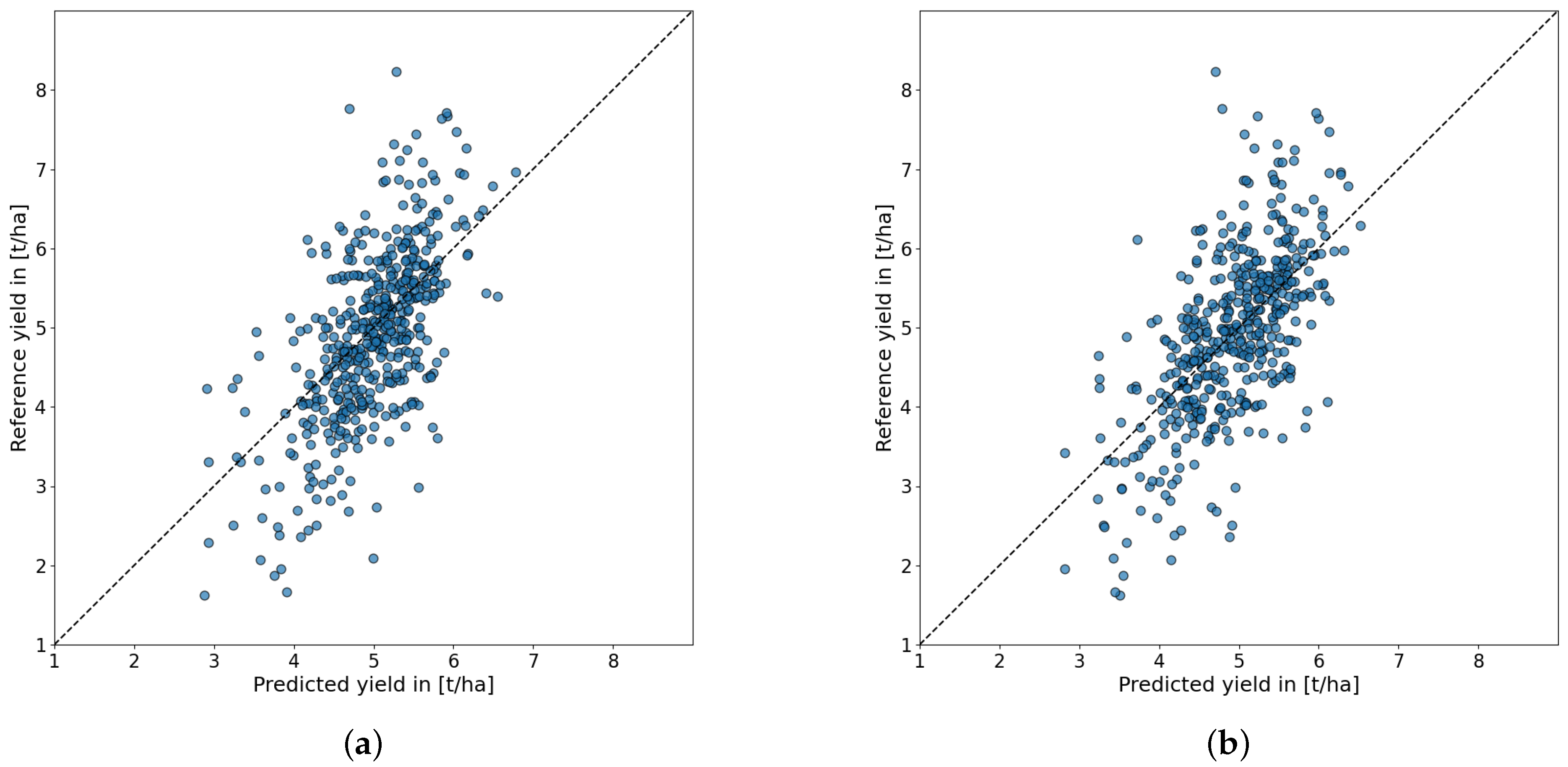
The first step was to analyze how much of the yield variability can be explained by SSM alone. For this purpose, the entire dataset was randomly divided into training and test data. One model was then trained with the H SAF product and one model with the ERA5 SWVL1 product, which were then subsequently evaluated. Table 1 shows the accuracy metrics achieved for the two models. The H SAF model achieved a PearsonR value of 0.59, an R2 value of 0.33, an RMSE of 0.89, and a MAE of 0.68. The values for the ERA5 model are slightly better for all metrics. The PearsonR for ERA5 SWVL1 is 0.61, the R2 0.37, RMSE 0.86 and MAE 0.65. The F-statistic for the ERA5 model is 9.9, and for the H SAF model 8.0. The H SAF SSM product can thus explain 33% of the variability in spring barley yield in the dataset and the ERA5 SWVL1 37% of the variability in spring barley yield. To test the significance of the achieved R2, we further calculated from the F-statistics the corresponding p-value for all model runs. The obtained p-values were all below the threshold of 0.05, indicating that the R2 value is statistically significant and unlikely to have occurred by chance. Figure 3a,b shows scatterplots for the predicted and reference yield for both models. Similar patterns can be recognized for both products: A good alignment between predicted, and reference yield can be observed especially for reference yields between 4 t/ha and 6 t/ha, whereas the models for both products tend to overestimate low yields and significantly underestimates high spring barley yields.

3.2. Spatial Evaluation of the Models

To assess the performance for the different geographic regions, a cross-validation was carried out on the NUTS level. Over three runs, samples of a different third of the 413 NUTS regions were used as a test dataset and the samples of the other two-thirds for training and validation. The experiment was repeated five times, each time using a different split to reduce the impact of the split on the accuracy metrics. To ensure comparable results, the same train-test split was used for both products. All predictions were then assigned to their corresponding NUTS region and country. For every NUTS region and the three countries, the final metrics were subsequently calculated over all assigned predictions.
Table 2 outlines the achieved metrics for the two models and the three countries. In Czechia, both models achieved very similar results, and each the lowest RMSE and MAE among the three countries. The ERA5 model achieved slightly higher values for PearsonR and R2. RMSE, ubRMSE and MAE are almost identical for both models. The metrics for Austria are significantly worse for both models. The H SAF model achieved a PearsonR of 0.50, an R2 of 0.17, and MAE of 0.70 t/ha. Here, the highest difference between the RMSE and the ubRMSE can be observed with values of 0.89 t/ha and 0.84 t/ha. The ERA5 model achieved slightly better metrics with a PearsonR of 0.53, an R2 of 0.23, and RMSE, respectively, MAE of 0.85 t/ha and 0.67 t/ha. The difference here between RMSE and ubRMSE is only 0.01 t/ha. The highest PearsonR and R2 for both products were achieved in Germany. The PearsonR for the H SAF model is 0.53 compared to 0.58 for the ERA5 model. Also, the R2 is 0.06 higher for the ERA5 model (0.34 to 0.28). The RMSE ubRMSE are both 0.05 t/ha lower and the MAE is 0.03 lower (0.69 t/ha to 0.72 t/ha) for the ERA5 model.
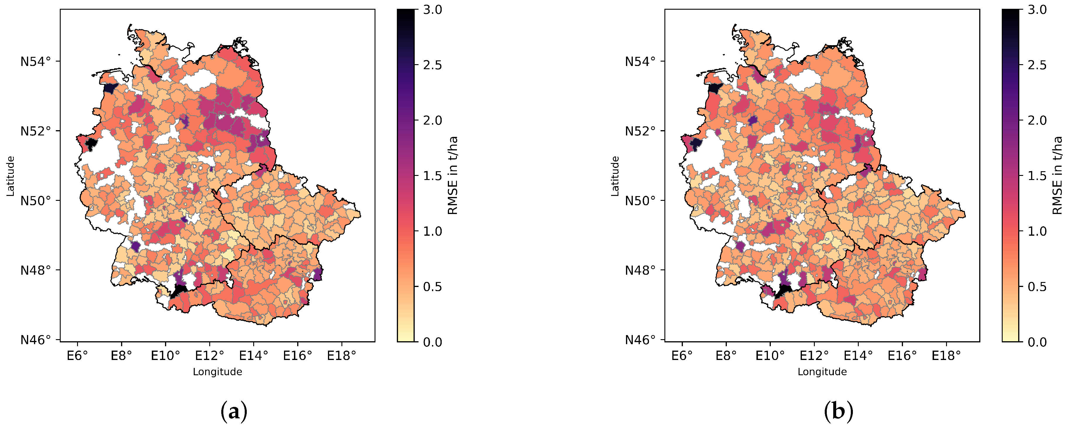
Figure 4 illustrates the RMSE on the country level for the H SAF product (a) and the ERA5 product (b). Overall, both products show similar spatial patterns. Outlier regions with very high RMSE values are located especially in Germany (NUTS regions DE94C, DEA1F, DE27B, DE258, DE298, DE12A). Moreover, both products show a cluster with high RMSE values in Eastern Germany, with slightly higher RMSE values for the H SAF product. The H SAF model shows some regions with higher values in the alpine regions in Southern Germany and Austria, which are less pronounced for the ERA5 model. In Czechia, both models show overall the lowest RMSE values with only one outlier region (CZ0421) at the border with Germany exceeding an RMSE of 1.5 t/ha.

3.3. Comparison of ERA5 SWVL1 and H SAF SSM

Figure 5 shows the differences between the predictions for the H SAF model and the ERA5 SWVL1 model per NUTS region. The figure was derived by calculating the RMSE difference between the prediction of the H SAF model and the ERA5 model, thus the difference between Figure 4a,b. Positive values in Figure 5 indicate higher errors for the H SAF-based model, whereas negative errors indicate higher errors for the ERA5-based models. To test if the differences between the RMSE values over the 50 runs of the H SAF model and ERA5 model are statistically significant, we performed a paired t-test between these values, using the p-value 0.05 as the threshold. The calculated p-value quantifies the statistical significance of the observed differences between the compared cases. Specifically, it represents the probability of obtaining the observed differences, or more extreme ones, under the null hypothesis that the means of the two groups being compared are identical. NUTS regions with significant differences are highlighted in Figure 5 with a grid pattern. Looking at the figure, two areas with high differences stand out. The first and smaller one is the alpine region in Southern Germany and Western Austria. Here, higher errors are observed for the H SAF-based product. The second cluster is in Eastern Germany. Here, again, the H SAF model shows higher RMSE values in several NUTS regions. Remarkably, in all of Czechia, both models show a very similar performance with only 13 NUTS regions showing significant differences with a p-value ≤ 0.05. All of these have an RMSE difference smaller than 0.5 t/ha. Also, in most of Western and Central Germany as well as most of Southern and Eastern Austria, only a few regions show significant differences. In total, 81 of the 413 NUTS regions, equal to 20%, show significant differences. Of these, 32 show a significantly higher average RMSE value for the ERA5 product, and 49 show a higher average RMSE value for the H SAF product.

4. Discussion

4.1. Value of SSM for Spring Barley Yield Prediction

In this section, the explained variability score will be discussed, and in a later section, the two products will be compared in detail. The relatively high explained variability scores of 33% and 37%, combined with the PearsonR values of 0.59, respectively, 0.61, stress the high importance of SSM for spring barley yield prediction. It must be taken into account here that the explained variability R2 refers to the proportion of the variance in the reference yield that is explained by the independent variable, in this case, the min, max, and mean SSM values of the model. It can thus be only a rough indicator of the real relationship between SSM and spring barley yield. The results align with a previous study from Středa et al. [14] who achieved an R2 of 27% between available water holding capacity and spring barley yield in Czechia. The remaining variability not explained by SSM can be attributed to several other factors. A big fraction can be assigned to other meteorological variables. In their study, Chmielewski and Köhn [59] could explain 60% of spring barley yield variability with meteorological variables. Yiğit et al. [60] observed an explained variability of 82% for meteorological variables (temperature, precipitation, potential evapotranspiration, global radiation, and climatic water balance) for winter and spring barley yield in Germany. Temperature and solar radiation can be seen as the largest contributing factors here [61]. Field experiments have shown that heat stress leads to a greater reduction in spring barley grain weight than water stress [62]. Besides meteorological variables, other contributing factors to be named here are soil acidity, fertility, and nutrient availability, particularly nitrogen and phosphorus are crucial [63]. Thai et al. [64] quantified the impact of fertilizer application on spring barley yield in a field experiment in Eastern Germany with 11%. The timing of sowing has been shown to impact yield, with early sowing leading to higher yields as long as young plants are not affected by frost [65]. Soil characteristics, including nitrogen content, impact yield to a certain degree [66]. Finally, effective disease control and genetic factors, such as variety adaptability and stress resistance, enhance resilience [60,67,68].
Similar studies have been carried out for maize, which is, in general, considered a more drought-sensitive crop. These studies showed a higher explained variability for SSM on the maize yield. NeSmith et al. [69] observed a yield reduction of up to 40% for water-deficit treated maize plants. In addition, Milics et al. [70] compared SM to maize yield in Hungary and obtained an R2 score of 0.5947.
The scatter plots in Section 3.1 further indicate that the yield prediction models struggle to predict low and high yield values. The estimation of extreme values is, in general, difficult for ML models. Since extreme values are typically underrepresented in the dataset, ML methods tend to learn mainly non-extreme data points [71]. This is also evident when looking at the spatial error distribution, as discussed next.

4.2. Spatial Error Distribution

Section 3.2 outlined significant differences between the countries in the study region, with the lowest RMSE value for both products observed in Czechia. This can be related to two factors: A comparison of Figure 1 and Figure 4 indicates that regions with average yield values close to the overall average (between 4 t/ha and 6 t/ha) have typically low error rates. In Czechia, all NUTS regions have average yield values between 3 t/ha and 7 t/ha. This can be seen as the main reason why this country has the lowest RMSE value among the three countries. The higher error rates for Austria and Germany can partly be attributed to regions with significantly higher RMSE values. Some of these are identical for both models and some are amplified in the predictions of only one model. The high error values (RMSE ≥ 2.5 t/ha) of the isolated NUTS regions in Western and Southern Germany (DE94C, DEA1F, DE27B, and DE258) and Austria (AT4708) are probably due to the unusually high or low crop yield in these NUTS regions. As Figure 1 illustrates, the NUTS regions DE94C, DEA1F, DE27B, and AT4708 are among those with the highest average yield in the entire study region. NUTS region DE258, on the other hand, has a below-average yield. It is striking that all these regions differ greatly from their neighboring regions in terms of yield. The low prediction accuracy of the SSM models and the isolated occurrence of these patterns lead to the conclusion that these deviations are not or only to a small extent attributable to SSM. More likely, there are causes that occur on a smaller scale, such as nutrient availability, differences in the form of cultivation, etc.
Table 2 indicates that Austria has, for both products, the lowest R2 and the highest difference between the RMSE and the ubRMSE. This indicates a significant bias in the predictions, which is also evident from Figure 4 where wide scale RMSE values around 1 t/ha) for both products are visible. On closer examination, it turns out this is caused by an overprediction of the spring barley yield. The cause of this can be seen in the unfavorable growing conditions mentioned in Section 2.1: frequent late frosts in the west and heavy soils in the east. Thus, the models struggle to predict the relatively low yield values based only on the SSM time series of the two products, leading to the low R2 values and the high RMSE. These unfavorable conditions are also reflected in a steady decrease in the production of spring barley and a transition to the cultivation of winter barley in Austria [37].
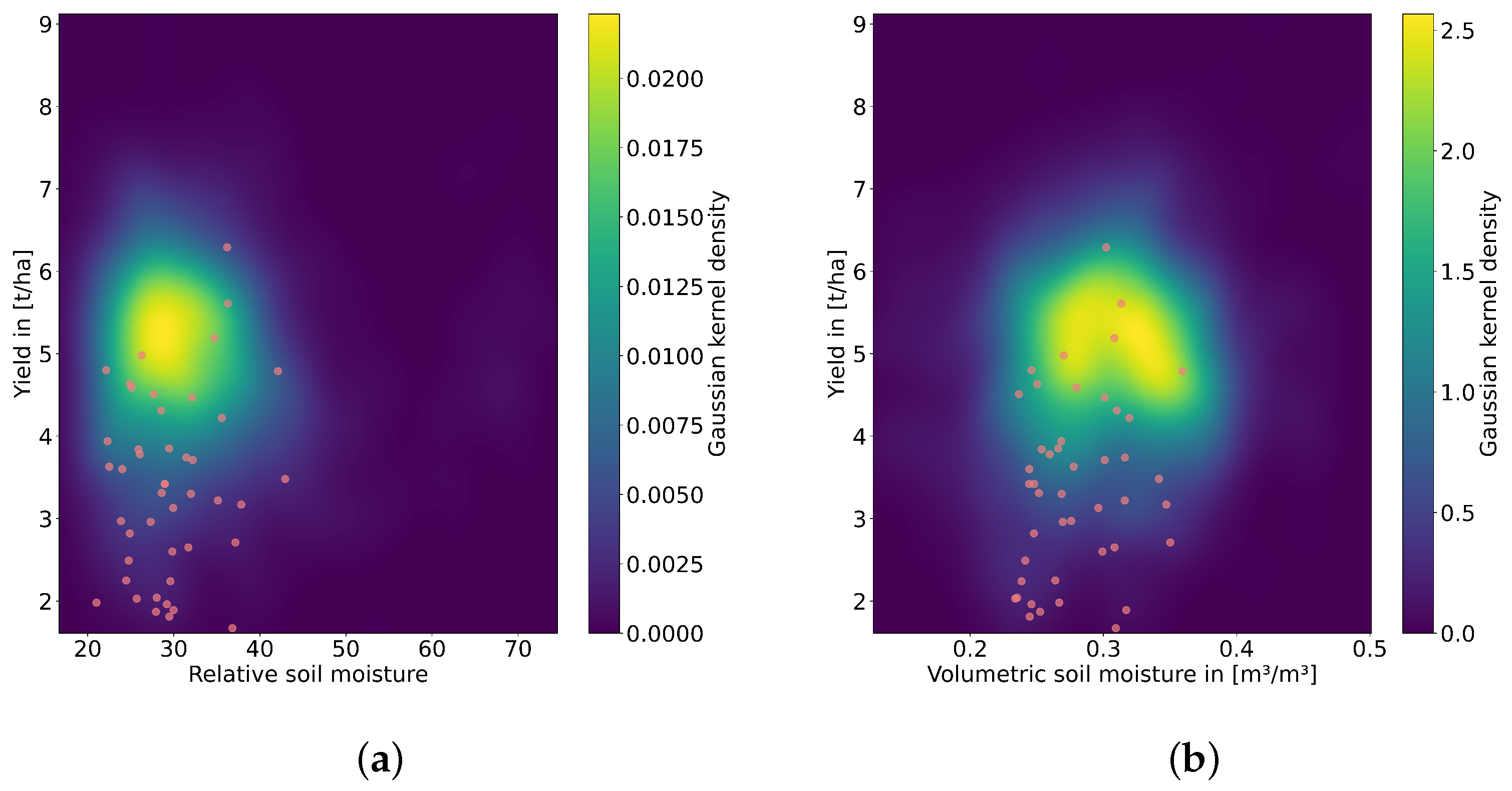
For both products, the highest RMSE errors occur in Eastern Germany, especially the NUTS regions DE405, DE40A, DE40E, DE40H, DE406, and DE40G. A closer look at the predictions for these regions reveals that they are strongly affected by a bias and a constant significant overprediction of yield. The obtained bias for these regions ranges from 1.8 t/ha to 2.9 t/ha. The ubRMSE for these NUTS regions is, thus, significantly lower and ranges from 0.4 t/ha to 1.3 t/ha. To better understand why the models for both products struggle to accurately predict spring barley yield based on SSM, we created density plots showing the yield and average SSM for the samples of the NUTS regions in Eastern Germany compared to the samples from all other NUTS regions. Figure 6 illustrates this for the two SSM products. As can be seen, the majority of the samples from the NUTS regions in Eastern Germany (displayed as red dots) have a (far) below-average yield. However, they mostly have average or only slightly below average SSM values. Based on this probability distribution, however, a significantly higher yield would be expected for the SSM values of most of these samples. It must be noted that this illustration only represents a simplified relationship between SSM and yield, as only the average SSM values for the entire growth phase are used here. We conclude from these that the relationship between SSM and yield in this region differs greatly from the rest of the study region. As a reason for this, we refer back to Section 2.1 that pointed out that this region is characterized by unfavorable cultivation conditions, with drier conditions and soils with lower water holding capacity [33]. Due to these unique conditions, both models have difficulties predicting the low yield there based on SSM. Here, the use of a root-zone SM might prove to be useful, as it would give more of an indication of how long water is available to plants. Nonetheless, reliable root-zone SM needs to be available that takes into account soil characteristics, which is currently not available from the H SAF product suite. Looking at the spatial errors, differences between the predictions of the models of the two SSM products become obvious and are discussed in the following section.

4.3. Comparison of the Two SSM Products

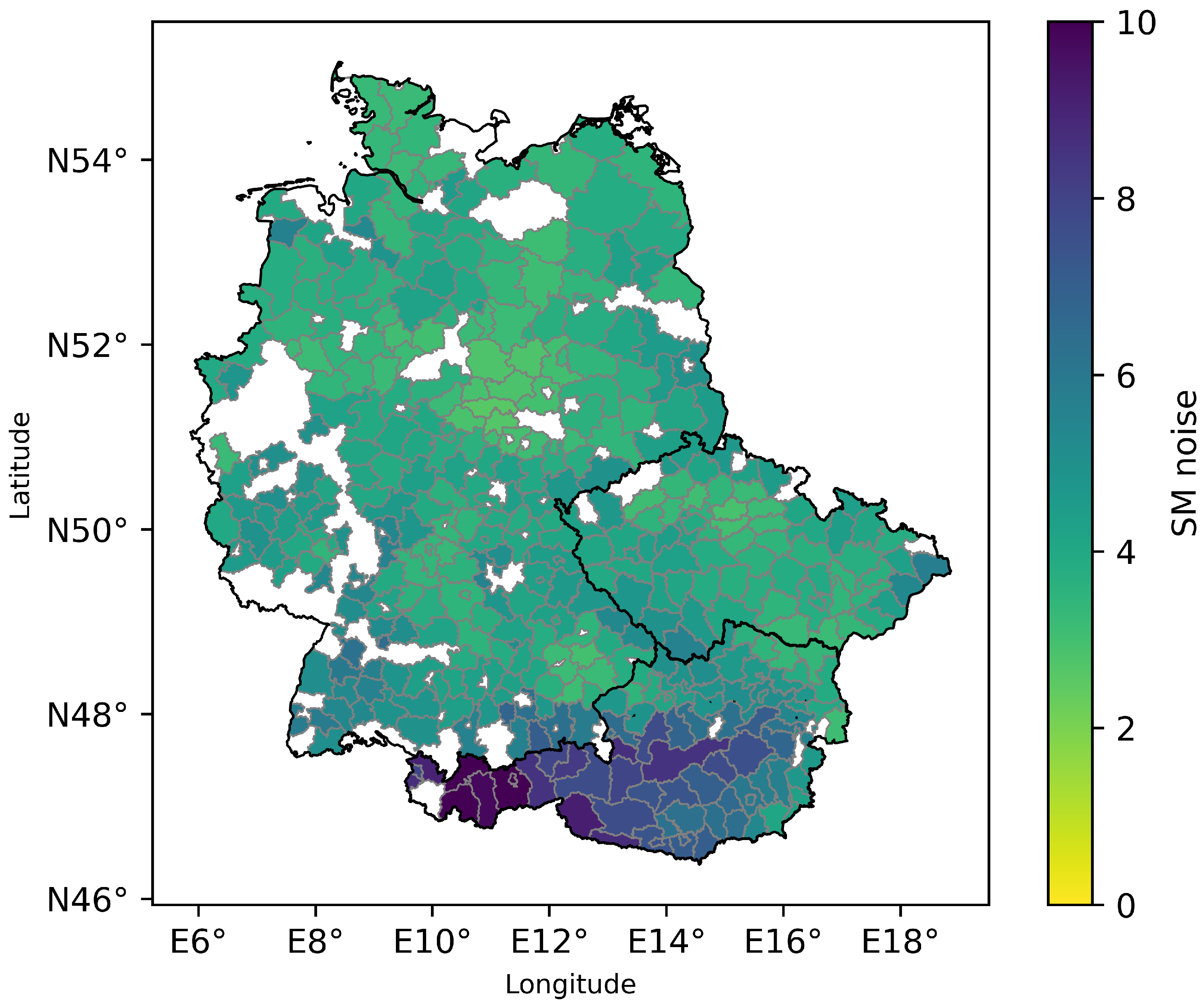
Section 3.1 and Section 3.2 have shown that the models for both products achieved very similar results for the random split as well as for the spatial split. In both cases, a (slightly) better performance was observed for the ERA5 SWVL1 product. As already mentioned in the introduction, the aim of this study was not a validation of the SM products. Studies validating the two SSM products with in-situ measurements observed a high agreement for both products in Europe with slightly lower errors for the ERA5 product [72,73]. Other studies compared the two products, respectively, the H SAF product with another model-based SSM product, for different applications: Modanesi et al. [74] found a higher correlation for satellite-derived SM products to crop losses compared to model-based SM products. Gaona et al. [75] concluded in their study that the H SAF product has a high value for drought monitoring in Europe. It must also be taken into account that the products are derived differently and depict SSM at different soil depths. While both products represent SSM, the ERA5 SWVL1 is defined to cover the depth up to 7 cm, while the H SAF product only covers the top 2 cm. Moreover, ERA5 SWVL1 is a model-derived product, whereas the H SAF product is derived from satellite data. Thus, the H SAF product captures, in contrast to the ERA5 product, irrigation. On the other hand, the ERA5 SWVL1 product is deduced using additional information like soil maps that can potentially be advantageous for yield prediction. In contrast, the derivation from satellite observations makes the H SAF product subject to influences stemming from different land covers, the satellite’s acquisition geometry, radio frequency interference, and other factors. These are mapped in the calculation of the SM noise. Figure 7 shows the average H SAF SM noise for all NUTS regions calculated for the same period as the SSM data. As the figure illustrates, the highest noise values can be found in the Alpine region. Here, the significant terrain causes uncertainties in the calculation of the SM. The higher error rates in the prediction using the H SAF product in some of the regions (AT4702, AT4701, AT4703, DE21F, DE21K, AT4506, AT4504, AT4612) in the Alpine area, illustrated in Figure 5, can thus be most likely related to high SM noise. This aligns with findings from previous studies. Hahn et al. [76] found that in mountainous terrain, the influence of ASCAT SM assimilation on precipitation forecasts was low, mainly due to forcing mechanisms specific to these regions. Paulik et al. [77] observed that the mountainous Southern part of their study area consistently showed higher topsoil moisture values compared to the northern part, indicating potential challenges in accurate SM retrieval in such terrain. Considering these partly high SM noise values in the study region and the significant differences in the retrieval and definition of the two products, it is remarkable that they achieved comparable results in 80% of the NUTS regions.
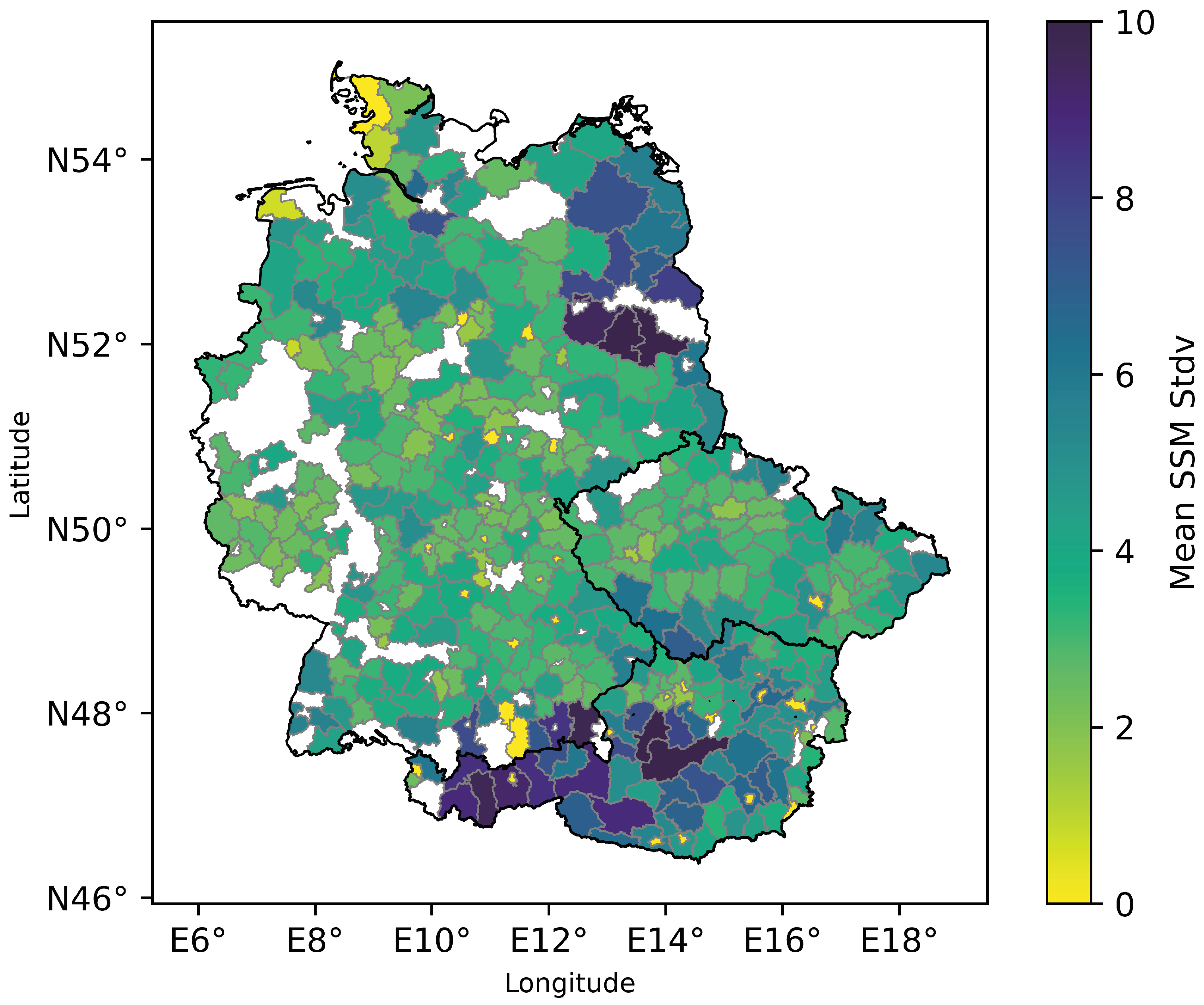
From Figure 7, we can also conclude that the significant differences in the RMSE values in Eastern Germany can not be attributed to SM noise. To inspect the reliability of the mean H SAF SSM time series of the NUTS region, we calculated the standard deviation per NUTS region. This was conducted by determining the daily standard deviation for the SSM time series of all grid points in the NUTS regions. The mean standard deviation over the entire year was then calculated for all years in which crop yield data were available for this NUTS region. The result is illustrated in Figure 8. This figure shows a strong overlap with Figure 5. Many NUTS regions in which the H SAF product has higher RMSE values also have high standard deviations. In the Alpine region, the high standard deviations can again be attributed to the high SM noise, as well as to small-scale differences in rainfall due to the effect of the mountains as a weather divide. In Eastern Germany, especially the regions DE405, DE40A, DE40E, DE40H, and DE406 show both a high standard deviation and a high RMSE value for the H SAF product. To understand what causes the high standard deviation in these regions, the deviations per grid point were determined in the regions. This revealed that grid points with a high difference from the mean SM are often located in forest areas or in the proximity of water bodies. A CORINE landcover-based calculation of forest cover per NUTS region showed that these NUTS regions have a high fraction of forest (between 40 and 50%) and a relatively low percentage of agriculture (between 30 and 50%). In addition, the two federal states Brandenburg and Mecklenburg-Vorpommern, in which these NUTS regions are located, are those with the highest number of lakes in Germany [78]. As densely vegetated areas and water bodies allow no (accurate) derivation of SM from microwave observation and, thus, no reliable SM retrieval, they contribute to the high variability within the NUTS region [79,80]. The high variability subsequently has the effect that the mean SM time series is less reliable in these NUTS regions. An improved selection of grid points based only on agriculture or filtering out grid points with a high derivation from the mean SSM would likely improve the yield prediction in the NUTS regions for the H SAF model.

4.4. Limitations of the Study

The findings of this study are subject to several limitations, which are discussed in the following. First, several factors can impact and potentially reduce the achieved explained variability for SSM: the quality of the SSM products, the quality of the yield data, the quality of the model fit, and in particular, the temporal and spatial resolution of the SSM. In addition, carrying out the analysis on the NUTS level without knowledge about the distribution of spring barley within the region introduces further uncertainties, especially with regard to the retrieval of the corresponding SSM time series. The real explained variability (as observed with in-situ measurements in a field study) of SSM can thus be even higher. Moreover, within this study, we only tested one satellite-based SM product and one model-based SM product. Other widely used active products, such as the CLMS Sentinel 1-based SSM product, passive products like ASMR2, or a combined product like SMAP, were not tested. However, based on previous studies [80,81,82], similar findings regarding performance limitations in low-sensitivity areas are expected, especially for c-band and x-band-based products. It must also be taken into account that the study region covers only a limited range of climate conditions. As the importance of individual factors is expected to be highly dependent on the climate conditions, the transferability to other regions is, therefore, limited. In regions with climate conditions similar to central Europe, for instance, parts of eastern North America, parts of East Asia or New Zealand, similar results for the explained variability can be expected. Ray et al. [83] analyzed the influence of climate variables (temperature, precipitation) on crop yield on a global scale and concluded that there are considerable spatial differences in their impact. In dry regions such as sub-Saharan Africa, SM is significantly more important. Gibon et al. [84] demonstrated this by quantifying the explained variability for SM on millet yield in the Sahel with 81%. In northern regions and regions where crops are typically irrigated, temperature has been shown to have a higher importance compared to SM [83].

5. Conclusions

In this study, we took a detailed look at the value of the two SSM products, H SAF and ERA5 SWVL1, for the prediction of spring barley yield in Central Europe. In this scope, we trained an FFNN using SSM time series and spring barley yield for NUTS3 regions in Germany and NUTS4 regions in Austria and the Czechia for the years 2016 to 2022. The results showed that SSM has a high potential to predict variability in spring barley yields. ERA5 SWVL1 can explain 37% and the H SAF product 33% of the yield variability in the crop. A spatial evaluation of the predictions of the two products revealed that they achieve similar RMSE values for Czechia and most parts of Germany and Austria. In the Alpine regions of Southern Germany and Western Austria, the H SAF product showed higher RMSE values in some NUTS regions, which can be attributed to the high SM noise in these regions. The biggest differences occurred in Eastern Germany. The H SAF product performed significantly worse here. Our analysis revealed that in these regions, the standard deviation of the SSM time series of the different grid points is higher than in the remaining study region. This can be attributed to the high fraction of dense vegetation and a high number of water bodies in these regions, which decrease the sensitivity of the radar signal to SSM. In these areas with low sensitivity of microwaves, the usage of model-based SSM such as ERA5 or improved filtering of the grid points is expected to increase the prediction accuracy. In the remaining study area, 80% of the NUTS regions, both products achieve comparable results. The H SAF product offers the advantage that it is provided in near real-time, thus allowing earlier predictions than the ERA5 reanalysis product. The usage of the latest version of the H SAF product, which includes several improvements such as a landcover-specific trend correction, could likely improve the results for this SSM product. Based on these results, adding SSM as an input to yield prediction or crop growth models for spring barley or similar crop types is recommended. In areas with low sensitivity for microwaves, model-based products are expected to allow more accurate results. Implementing these findings allows the development of more accurate yield prediction and crop growth models, subsequently contributing to more improved agricultural management and food security. These become increasingly relevant as droughts are expected to occur more frequently in Central Europe due to climate change. In this context, future work will focus on assessing in detail the performance in single years to understand the value of SSM under a variety of drought conditions.

Author Contributions

Conceptualization, F.R. and W.W.; methodology, F.R.; software, F.R.; validation, F.R.; formal analysis, F.R.; investigation, F.R.; resources, F.R.; data curation, F.R.; writing—original draft preparation, F.R.; writing—review and editing, F.R., M.V., E.B. and W.W.; visualization, F.R.; supervision, W.W.; project administration, E.B.; funding acquisition, E.B and M.V. All authors have read and agreed to the published version of the manuscript.

Funding

This study has been funded by the European Space Agency (ESA) in the framework of the project “YIPEEO: Yield prediction and estimation using Earth Observation”, contract number 4000141154/23/I-EF.

Data Availability Statement

Dataset available on request from the authors.

Acknowledgments

The authors would like to thank Sebastian Hahn for advice on the extraction of the H SAF SSM time series and for discussions on the interpretation of the results. We acknowledge CzechGlobe, ZALF, and Statistik Austria for providing the yield data. The authors also acknowledge TU Wien Bibliothek for financial support through its Open Access Funding Programme. Open Access Funding by TU Wien.

Conflicts of Interest

The authors declare no conflicts of interest.

Abbreviations

The following abbreviations are used in this manuscript:
ANNArtifical Neural Network
ASCATAdvanced Scatterometer
ATAustria
CZCzechia
DEGermany
ECMWFEuropean Centre for Medium-Range Weather Forecasts
EUMETSATEuropean Organisation for the Exploitation of Meteorological Satellites
FFNNFeed-Forward Neural Network
H SAFEUMETSAT Satellite Application Facility on Support to Operational Hydrology and Water Management
MAEMean Absolute Error
MLMachine Learning
NUTSNomenclature Des Unités Territoriales Statistiques
RMSERoot Mean Square Error
SMSoil Moisture
SSMSurface Soil Moisture
SWISoil Water Index
SWVL1Volumetric Soil Water Layer 1
ubRMSEunbiased Root Mean Square Error

References

  1. Shah, A.; Dubey, A.; Hemnani, V.; Gala, D.; Kalbande, D.R. Smart Farming System: Crop Yield Prediction Using Regression Techniques. In Proceedings of the International Conference on Wireless Communication, Mumbai, India, 19–20 January 2018; Vasudevan, H., Deshmukh, A.A., Ray, K.P., Eds.; Springer: Singapore, 2018; pp. 49–56. [Google Scholar] [CrossRef]
  2. Jang, S.J.; Kim, J.S.; Kim, T.W.; Lee, H.J.; Ko, S. A Wafer Map Yield Prediction Based on Machine Learning for Productivity Enhancement. IEEE Trans. Semicond. Manuf. 2019, 32, 400–407. [Google Scholar] [CrossRef]
  3. Kumar, R.; Singh, M.; Kumar, P.; Singh, J. Crop Selection Method to maximize crop yield rate using machine learning technique. In Proceedings of the 2015 International Conference on Smart Technologies and Management for Computing, Communication, Controls, Energy and Materials (ICSTM), Chennai, India, 6–8 May 2015; pp. 138–145. [Google Scholar] [CrossRef]
  4. Zaloom, C. How to Read the Future: The Yield Curve, Affect, and Financial Prediction. Public Cult. 2009, 21, 245–268. [Google Scholar] [CrossRef]
  5. Mahmoodi-Eshkaftaki, M.; Rafiee, M.R. Optimization of irrigation management: A multi-objective approach based on crop yield, growth, evapotranspiration, water use efficiency and soil salinity. J. Clean. Prod. 2020, 252, 119901. [Google Scholar] [CrossRef]
  6. Lukina, E.V.; Freeman, K.W.; Wynn, K.J.; Thomason, W.E.; Mullen, R.W.; Stone, M.L.; Solie, J.B.; Klatt, A.R.; Johnson, G.V.; Elliott, R.L.; et al. Nitrogen fertilization optimization algorithm based on In-Season estimates of yield and plant nitrogen uptake. J. Plant Nutr. 2001, 24, 885–898. [Google Scholar] [CrossRef]
  7. Chen, C.; Wang, X.; Chen, H.; Wu, C.; Mafarja, M.; Turabieh, H. Towards Precision Fertilization: Multi-Strategy Grey Wolf Optimizer Based Model Evaluation and Yield Estimation. Electronics 2021, 10, 2183. [Google Scholar] [CrossRef]
  8. Felix Kogan, W.G.; Yang, W. Drought and food security prediction from NOAA new generation of operational satellites. Geomat. Nat. Hazards Risk 2019, 10, 651–666. [Google Scholar] [CrossRef]
  9. Kang, Y.; Khan, S.; Ma, X. Climate change impacts on crop yield, crop water productivity and food security—A review. Prog. Nat. Sci. 2009, 19, 1665–1674. [Google Scholar] [CrossRef]
  10. Kumar, M. Impact of climate change on crop yield and role of model for achieving food security. Environ. Monit. Assess. 2016, 188, 465. [Google Scholar] [CrossRef]
  11. Eurostat. Agricultural Production—Crops. Available online: https://ec.europa.eu/eurostat/statistics-explained/index.php?title=Agricultural_production_-_crops#Cereals (accessed on 16 October 2024).
  12. Verstegen, H.; Köneke, O.; Korzun, V.; von Broock, R. The World Importance of Barley and Challenges to Further Improvements. In Biotechnological Approaches to Barley Improvement; Springer: Berlin/Heidelberg, Germany, 2014; pp. 3–19. [Google Scholar] [CrossRef]
  13. Day, A.D.; Thompson, R.K. Effects of Soil-Moisture Regimes on the Growth of Barley. Agron. J. 1975, 67, 430–433. [Google Scholar] [CrossRef]
  14. Streda, T.; Stredova, H.; Kohut, M.; Roznovsky, J.; Bougares, F.; Schwenk, H.; Bengio, Y. Yield of spring barley in dependence of soil moisture balance. In Proceedings of the 61. Tagung der Vereinigung der Pflanzenzüchter und Saatgutkaufleute Österreichs 2010, Raumberg-Gumpenstein, Austria, 23–25 November 2010; Vereinigung der Pfl anzenzüchter und Saatgutkaufleute: Vienna, Austria, 2011; pp. 171–174. [Google Scholar]
  15. Parkinson, K.J.; Day, W. The Influence of Water Stress on Photosynthesis in a Barley Crop. In Effects of Stress on Photosynthesis: Proceedings of a Conference Held at the ‘Limburgs Universitair Centrum’ Diepenbeek, Belgium, 22–27 August 1982; Marcelle, R., Clijsters, H., van Poucke, M., Eds.; Springer: Dordrecht, The Netherlands, 1983; pp. 65–74. [Google Scholar] [CrossRef]
  16. Power, J.F.; Grunes, D.L.; Reichman, G.A. The Influence of Phosphorus Fertilization and Moisture on Growth and Nutrient Absorption by Spring Wheat: I. Plant Growth, N Uptake, and Moisture Use. Soil Sci. Soc. Am. J. 1961, 25, 207–210. [Google Scholar] [CrossRef]
  17. Hargreaves, G.H. Moisture Availability and Crop Production. Trans. ASAE 2013, 18, 980–984. [Google Scholar] [CrossRef]
  18. Zhao, F.; Wang, G.; Li, S.; Hagan, D.F.T.; Ullah, W. The combined effects of VPD and soil moisture on historical maize yield and prediction in China. Front. Environ. Sci. 2023, 11, 1117184. [Google Scholar] [CrossRef]
  19. Bushong, J.T.; Mullock, J.L.; Miller, E.C.; Raun, W.R.; Klatt, A.R.; Arnall, D.B. Development of an in-season estimate of yield potential utilizing optical crop sensors and soil moisture data for winter wheat. Precis. Agric. 2016, 17, 451–469. [Google Scholar] [CrossRef]
  20. White, J.; Berg, A.A.; Champagne, C.; Zhang, Y.; Chipanshi, A.; Daneshfar, B. Improving crop yield forecasts with satellite-based soil moisture estimates: An example for township level canola yield forecasts over the Canadian Prairies. Int. J. Appl. Earth Obs. Geoinf. 2020, 89, 102092. [Google Scholar] [CrossRef]
  21. Bueechi, E.; Fischer, M.; Crocetti, L.; Trnka, M.; Grlj, A.; Zappa, L.; Dorigo, W. Crop yield anomaly forecasting in the Pannonian basin using gradient boosting and its performance in years of severe drought. Agric. For. Meteorol. 2023, 340, 109596. [Google Scholar] [CrossRef]
  22. Boas, T.; Bogena, H.R.; Ryu, D.; Vereecken, H.; Western, A.; Hendricks Franssen, H.J. Seasonal soil moisture and crop yield prediction with fifth-generation seasonal forecasting system (SEAS5) long-range meteorological forecasts in a land surface modelling approach. Hydrol. Earth Syst. Sci. 2023, 27, 3143–3167. [Google Scholar] [CrossRef]
  23. Bojanowski, J.S.; Sikora, S.; Musiał, J.P.; Woźniak, E.; Dąbrowska-Zielińska, K.; Slesiński, P.; Milewski, T.; Łączyński, A. Integration of Sentinel-3 and MODIS Vegetation Indices with ERA-5 Agro-Meteorological Indicators for Operational Crop Yield Forecasting. Remote Sens. 2022, 14, 1238. [Google Scholar] [CrossRef]
  24. Ines, A.V.; Das, N.N.; Hansen, J.W.; Njoku, E.G. Assimilation of remotely sensed soil moisture and vegetation with a crop simulation model for maize yield prediction. Remote Sens. Environ. 2013, 138, 149–164. [Google Scholar] [CrossRef]
  25. Potopová, V.; Trnka, M.; Hamouz, P.; Soukup, J.; Castraveț, T. Statistical modelling of drought-related yield losses using soil moisture-vegetation remote sensing and multiscalar indices in the south-eastern Europe. Agric. Water Manag. 2020, 236, 106168. [Google Scholar] [CrossRef]
  26. Saf, H. EUMETSAT SAF on Support to Operational Hydrology and Water Management. ASCAT Surface Soil Moisture Climate Data Record v7 12.5 km Sampling—Metop. 2021. Available online: https://user.eumetsat.int/catalogue/EO:EUM:DAT:0656 (accessed on 19 August 2024).
  27. C3S. ERA5 Hourly Data on Single Levels from 1940 to Present; C3S: Chennai, India, 2015. [Google Scholar] [CrossRef]
  28. Guitard, A.A. The Influence of Variety, Temperature, and Stage of Growth on the Response of Spring Barley to Photoperiod. Can. J. Plant Sci. 1960, 40, 65–80. [Google Scholar] [CrossRef]
  29. Svobodová, I.; Misa, P. Effect of drought stress on the formation of yield elements in spring barley and the potential of stress expression reduction by foliar application of fertilizers and growth stimulator. Plant Soil Environ. 2004, 50, 439–446. [Google Scholar] [CrossRef]
  30. Hlavinka, P.; Trnka, M.; Eitzinger, J.; Smutny, V.; Thaler, S.; Žalud, Z.; Rischbeck, P.; Kren, J. The performance of CERES-Barley and CERES-Wheat under various soil conditions and tillage practices in Central Europe. Die Bodenkult. 2010, 61, 5–17. [Google Scholar]
  31. Eitzinger, J.; Kubu, G.; Thaler, S. Climate Change Impacts And Adaptation Options for Agriculture in Complex Terrain and Small Scale Agricultural Systems—Results from Case Studies in Austria. In Proceedings of the Extended Abstracts of the International Symosium, University of Natural Resources and Applied Life Sciences (BOKU); Eitzinger, J., Kubu, G., Eds.; University of Natural Resources and Applied Life Sciences (BOKU): Vienna, Austria, 2009; Volume 6, p. 159. [Google Scholar]
  32. Eitzinger, J.; Daneu, V.; Bodner, G.; Kubu, G.; Loiskandl, W.; Macaigne, P.; Thaler, S.; Schaumberger, A.; Wittmann, C.; Weidle, F.; et al. Drought Monitoring System for Austrian Agriculture—AgroDroughtAustria (Final Scientific Report of Project “AgroDroughtAustria” of the Austrian Climate Change Research Program; Technical Report; University of Natural Resources and Applied Life Sciences (BOKU): Vienna, Austria, 2016. [Google Scholar]
  33. Grosse, M.; Hierold, W.; Ahlborn, M.C.; Piepho, H.P.; Helming, K. Long-term field experiments in Germany: Classification and spatial representation. Soil 2020, 6, 579–596. [Google Scholar] [CrossRef]
  34. Váňová, M.; Palík, S.; Hajšlová, J.; Burešová, I. Grain quality and yield of spring barley in field trials under variable growing conditions. Plant Soil Environ. 2006, 52, 211–219. [Google Scholar] [CrossRef]
  35. Gebeltová, Z. Exploitation of Agricultural Land in the Czech Republic and EU Countries. AGRIS On-Line Pap. Econ. Inform. 2017, 9, 33–44. [Google Scholar] [CrossRef]
  36. Brumer, A.; Wezel, A.; Dauber, J.; Breland, T.A.; Grard, B. Development of agroecology in Austria and Germany. Open Res. Eur. 2023, 3, 25. [Google Scholar] [CrossRef] [PubMed]
  37. Bundesministerium für Ernährung und Landwirtschaft. Cereal Production and Types of Cereals in Austria. Available online: https://info.bml.gv.at/en/topics/agriculture/agriculture-in-austria/plant-production-in-austria/cereal-production-and-types-of-cereals-in-austria.html (accessed on 22 January 2025).
  38. Janovska, V.; Simova, P.; Vlasak, J.; Sklenicka, P. Factors affecting farm size on the European level and the national level of the Czech Republic. Agric. Econ. 2017, 63, 1–12. [Google Scholar] [CrossRef]
  39. Vaishar, A.A.; Šťastná, M.A. Transformation of agriculture in Czechia in the period 1990–2020. Studia Obszarów Wiejskich 2020, 56, 103–118. [Google Scholar] [CrossRef]
  40. Office, C.S. Harvest Estimates—June 2024. Available online: https://csu.gov.cz/rychle-informace/harvest-estimates-june-2024l (accessed on 16 March 2025).
  41. Jasib, L.; Donnellan, T.; Lennon, J. The Inequality of Farmland Size in Western Europe. In Proceedings of the Agricultural Economics Society—AES > 90th Annual Conference, Dublin, Ireland, 24–26 April 2017. [Google Scholar] [CrossRef]
  42. Zakrzewska, A.; Nowak, A. Diversification of Agricultural Output Intensity across the European Union in Light of the Assumptions of Sustainable Development. Agriculture 2022, 12, 1370. [Google Scholar] [CrossRef]
  43. Wagner, W.; Lemoine, G.; Rott, H. A Method for Estimating Soil Moisture from ERS Scatterometer and Soil Data. Remote Sens. Environ. 1999, 70, 191–207. [Google Scholar] [CrossRef]
  44. Naeimi, V.; Scipal, K.; Bartalis, Z.; Hasenauer, S.; Wagner, W. An Improved Soil Moisture Retrieval Algorithm for ERS and METOP Scatterometer Observations. IEEE Trans. Geosci. Remote Sens. 2009, 47, 1999–2013. [Google Scholar] [CrossRef]
  45. Hersbach, H.; Bell, B.; Berrisford, P.; Hirahara, S.; Horányi, A.; Muñoz-Sabater, J.; Nicolas, J.; Peubey, C.; Radu, R.; Schepers, D.; et al. The ERA5 global reanalysis. Q. J. R. Meteorol. Soc. 2020, 146, 1999–2049. [Google Scholar] [CrossRef]
  46. Fan, Y.; Liu, Y.; Yue, J.; Jin, X.; Chen, R.; Bian, M.; Ma, Y.; Yang, G.; Feng, H. Estimation of potato yield using a semi-mechanistic model developed by proximal remote sensing and environmental variables. Comput. Electron. Agric. 2024, 223, 109117. [Google Scholar] [CrossRef]
  47. Gómez, D.; Salvador, P.; Sanz, J.; Casanova, J.L. Modelling wheat yield with antecedent information, satellite and climate data using machine learning methods in Mexico. Agric. For. Meteorol. 2021, 300, 108317. [Google Scholar] [CrossRef]
  48. De Clercq, D.; Mahdi, A. Feasibility of machine learning-based rice yield prediction in India at the district level using climate reanalysis and remote sensing data. Agric. Syst. 2024, 220, 104099. [Google Scholar] [CrossRef]
  49. Lawrence, J. Introduction to Neural Networks; California Scientific Software: Saratoga, CA, USA, 1993. [Google Scholar]
  50. Kim, N.; Ha, K.J.; Park, N.W.; Cho, J.; Hong, S.; Lee, Y.W. A Comparison Between Major Artificial Intelligence Models for Crop Yield Prediction: Case Study of the Midwestern United States, 2006–2015. ISPRS Int. J.-Geo-Inf. 2019, 8, 240. [Google Scholar] [CrossRef]
  51. Kaul, M.; Hill, R.L.; Walthall, C. Artificial neural networks for corn and soybean yield prediction. Agric. Syst. 2005, 85, 1–18. [Google Scholar] [CrossRef]
  52. Ji, B.; Sun, Y.; Yang, S.; Wan, J. Artificial neural networks for rice yield prediction in mountainous regions. J. Agric. Sci. 2007, 145, 249–261. [Google Scholar] [CrossRef]
  53. Kingma, D.P.; Ba, J. Adam: A Method for Stochastic Optimization. arXiv 2017, arXiv:1412.6980. [Google Scholar]
  54. Chollet, F. Keras; GitHub: San Francisco, CA, USA, 2015. [Google Scholar]
  55. Entekhabi, D.; Njoku, E.G.; O’Neill, P.E.; Kellogg, K.H.; Crow, W.T.; Edelstein, W.N.; Entin, J.K.; Goodman, S.D.; Jackson, T.J.; Johnson, J.; et al. The Soil Moisture Active Passive (SMAP) Mission. Proc. IEEE 2010, 98, 704–716. [Google Scholar] [CrossRef]
  56. Zar, J.H. Spearman rank correlation. In Encyclopedia of Biostatistics; Wiley: Hoboken, NJ, USA, 2005; Volume 7. [Google Scholar]
  57. Wright, S. Correlation and causation. J. Agric. Res. 1921, 20, 557. [Google Scholar]
  58. Olson, C.L. On choosing a test statistic in multivariate analysis of variance. Psychol. Bull. 1976, 83, 579–586. [Google Scholar] [CrossRef]
  59. Chmielewski, F.M.; Köhn, W. Impact of weather on yield components of spring cereals over 30 years. Agric. For. Meteorol. 1999, 96, 49–58. [Google Scholar] [CrossRef]
  60. Yiğit, A.; Chmielewski, F.M. A Deeper Insight into the Yield Formation of Winter and Spring Barley in Relation to Weather and Climate Variability. Agronomy 2024, 14, 1503. [Google Scholar] [CrossRef]
  61. Trnka, M.; Eitzinger, J.; Kapler, P.; Dubrovský, M.; Semerádová, D.; Žalud, Z.; Formayer, H. Effect of Estimated Daily Global Solar Radiation Data on the Results of Crop Growth Models. Sensors 2007, 7, 2330–2362. [Google Scholar] [CrossRef] [PubMed]
  62. Savin, R.; Nicolas, M.E. Effects of timing of heat stress and drought on growth and quality of barley grains. Aust. J. Agric. Res. 1999, 50, 357. [Google Scholar] [CrossRef]
  63. Groß, J.; Gentsch, N.; Boy, J.; Heuermann, D.; Schweneker, D.; Feuerstein, U.; Brunner, J.; Von Wirén, N.; Guggenberger, G.; Bauer, B. Influence of small-scale spatial variability of soil properties on yield formation of winter wheat. Plant Soil 2023, 493, 79–97. [Google Scholar] [CrossRef]
  64. Thi Huyen, T.; Sonoko, D.; Bellingrath-Kimura, C.H.; Barkusky, D. Effect of long-term fertiliser regimes and weather on spring barley yields in sandy soil in North-East Germany. Arch. Agron. Soil Sci. 2020, 66, 1812–1826. [Google Scholar] [CrossRef]
  65. Appiah, M.; Bracho-Mujica, G.; Ferreira, N.C.; Schulman, A.H.; Rötter, R.P. Projected impacts of sowing date and cultivar choice on the timing of heat and drought stress in spring barley grown along a European transect. Field Crops Res. 2023, 291, 108768. [Google Scholar] [CrossRef]
  66. Finke, P.A.; Goense, D. Differences in barley grain yields as a result of soil variability. J. Agric. Sci. 1993, 120, 171–180. [Google Scholar] [CrossRef]
  67. Bondareva, L.; Danilov, D.; Kartashova, L. Breeding spring barley for ecological plasticity and adaptability in the North-Western Region. BIO Web Conf. 2020, 27, 00067. [Google Scholar] [CrossRef]
  68. Hlisnikovský, L.; Zemanová, V.; Roman, M.; Menšík, L.; Kunzová, E. Long-Term Study of the Effects of Environment, Variety, and Fertilisation on Yield and Stability of Spring Barley Grain. Plants 2024, 13, 2745. [Google Scholar] [CrossRef] [PubMed]
  69. NeSmith, D.; Ritchie, J. Maize (Zea mays L.) response to a severe soil water-deficit during grain-filling. Field Crops Res. 1992, 29, 23–35. [Google Scholar] [CrossRef]
  70. Milics, G.; Kovács, A.J.; Pörneczi, A.; Nyéki, A.; Varga, Z.; Nagy, V.; Lichner, L.; Németh, T.; Baranyai, G.; Neményi, M. Soil moisture distribution mapping in topsoil and its effect on maize yield. Biologia 2017, 72, 847–853. [Google Scholar] [CrossRef]
  71. Ding, D.; Zhang, M.; Pan, X.; Yang, M.; He, X. Modeling extreme events in time series prediction. In Proceedings of the 25th ACM SIGKDD International Conference on Knowledge Discovery & Data Mining, Anchorage, AK, USA, 4–8 August 2019; pp. 1114–1122. [Google Scholar]
  72. Pierdicca, N.; Fascetti, F.; Pulvirenti, L.; Crapolicchio, R.; Muñoz-Sabater, J. Quadruple Collocation Analysis for Soil Moisture Product Assessment. IEEE Geosci. Remote Sens. Lett. 2015, 12, 1595–1599. [Google Scholar] [CrossRef]
  73. Pierdicca, N.; Fascetti, F.; Pulvirenti, L.; Crapolicchio, R.; Muñoz-Sabater, J. Analysis of ASCAT, SMOS, in-situ and land model soil moisture as a regionalized variable over Europe and North Africa. Remote Sens. Environ. 2015, 170, 280–289. [Google Scholar] [CrossRef]
  74. Modanesi, S.; Massari, C.; Camici, S.; Brocca, L.; Amarnath, G. Do Satellite Surface Soil Moisture Observations Better Retain Information About Crop-Yield Variability in Drought Conditions? Water Resour. Res. 2020, 56, e2019WR025855. [Google Scholar] [CrossRef]
  75. Gaona, J.; Bavera, D.; Fioravanti, G.; Hahn, S.; Stradiotti, P.; Filippucci, P.; Camici, S.; Ciabatta, L.; Mossaffa, H.; Puca, S.; et al. Soil moisture products consistency for operational drought monitoring in Europe. Hydrol. Earth Syst. Sci. Discuss. 2024, 1–36. [Google Scholar] [CrossRef]
  76. Hahn, S.; Melzer, T.; Wagner, W. Error Assessment of the Initial Near Real-Time METOP ASCAT Surface Soil Moisture Product. IEEE Trans. Geosci. Remote Sens. 2012, 50, 2556–2565. [Google Scholar] [CrossRef]
  77. Paulik, C.; Dorigo, W.; Wagner, W.; Kidd, R. Validation of the ASCAT Soil Water Index using in situ data from the International Soil Moisture Network. Int. J. Appl. Earth Obs. Geoinf. 2014, 30, 1–8. [Google Scholar] [CrossRef]
  78. Hemm, M.; Hoffmann, A.; Mischke, U.; Nixdorf, B. Natürliche Seen Deutschlands—Aktueller Stand zur Dokumentation, Typisierung und Bewertung anhand des Phytoplanktons; Technical Report; Deutsche Gesellschaft für Limnologie (DGL): Essen, Germany, 2002. [Google Scholar]
  79. Dorigo, W.; Wagner, W.; Albergel, C.; Albrecht, F.; Balsamo, G.; Brocca, L.; Chung, D.; Ertl, M.; Forkel, M.; Gruber, A.; et al. ESA CCI Soil Moisture for improved Earth system understanding: State-of-the art and future directions. Remote Sens. Environ. 2017, 203, 185–215. [Google Scholar] [CrossRef]
  80. Massart, S.; Vreugdenhil, M.; Bauer-Marschallinger, B.; Navacchi, C.; Raml, B.; Wagner, W. Mitigating the impact of dense vegetation on the Sentinel-1 surface soil moisture retrievals over Europe. Eur. J. Remote Sens. 2024, 57, 2300985. [Google Scholar] [CrossRef]
  81. Kerr, Y.; Al-Yaari, A.; Rodriguez-Fernandez, N.; Parrens, M.; Molero, B.; Leroux, D.; Bircher, S.; Mahmoodi, A.; Mialon, A.; Richaume, P.; et al. Overview of SMOS performance in terms of global soil moisture monitoring after six years in operation. Remote Sens. Environ. 2016, 180, 40–63. [Google Scholar] [CrossRef]
  82. Njoku, E.; Jackson, T.; Lakshmi, V.; Chan, T.; Nghiem, S. Soil moisture retrieval from AMSR-E. IEEE Trans. Geosci. Remote Sens. 2003, 41, 215–229. [Google Scholar] [CrossRef]
  83. Ray, D.K.; Gerber, J.S.; MacDonald, G.K.; West, P.C. Climate variation explains a third of global crop yield variability. Nat. Commun. 2015, 6, 5989. [Google Scholar] [CrossRef]
  84. Gibon, F.; Pellarin, T.; Román-Cascón, C.; Alhassane, A.; Traoré, S.; Kerr, Y.; Lo Seen, D.; Baron, C. Millet yield estimates in the Sahel using satellite derived soil moisture time series. Agric. For. Meteorol. 2018, 262, 100–109. [Google Scholar] [CrossRef]
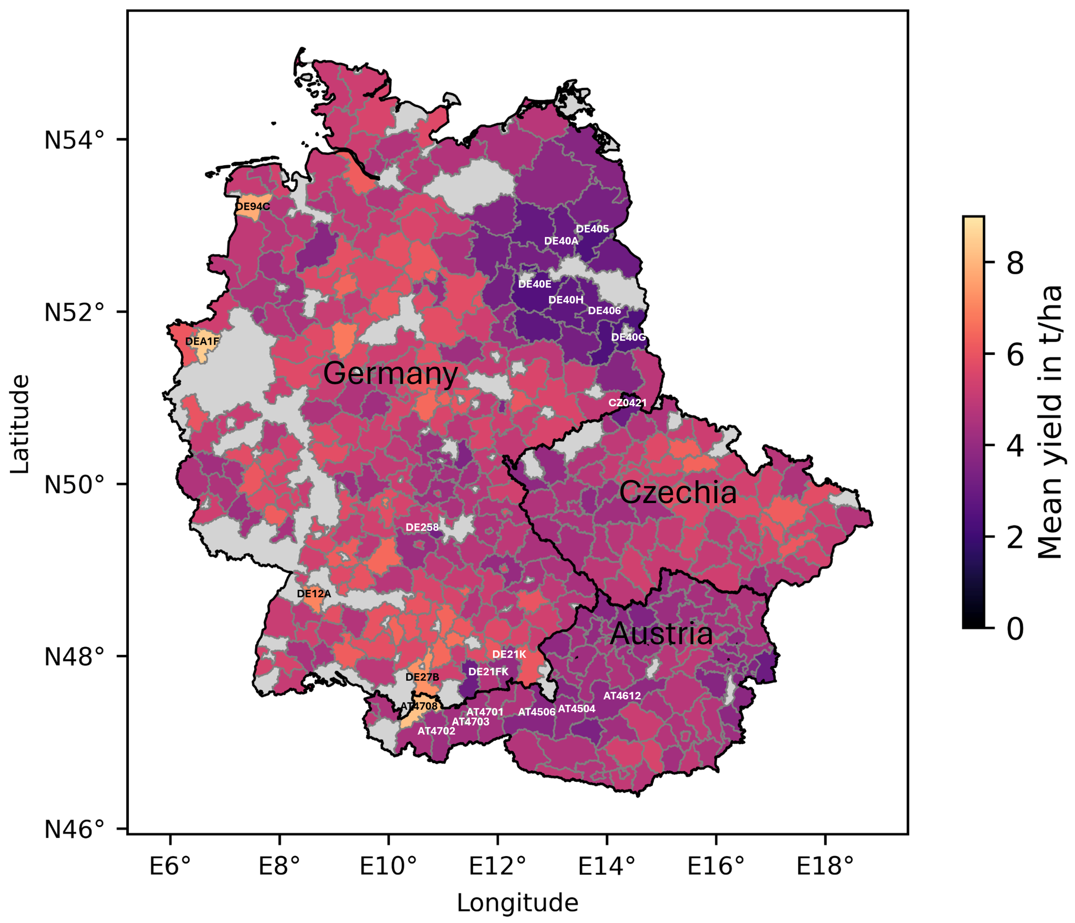
Figure 1. Illustration of the study region. The NUTS regions are shown with the average spring barley yield over the years 2016–2022 in tonnes/hectares. NUTS regions that are mentioned in the manuscript are labeled with their NUTS code. The color variations of the labels are used to enhance readability.
Remotesensing 17 01394 g001
Figure 2. The figure shows a simplified illustration of the architecture of the FFNN model. In addition, the model inputs and outputs are illustrated in their data shape. Depending on whether H SAF or ERA5 SSM is used, the models are referred to as H SAF or ERA5 model.
Remotesensing 17 01394 g002
Figure 3. Scatterplot between the predicted and the reference yield for the H SAF SSM and ERA5 SWVL1 product. The points always represent the average predicted yield over the ten runs. (a) H SAF SSM. (b) ERA5 SWVL1.
Remotesensing 17 01394 g003
Figure 4. RMSE between the predicted and reference yield for the H SAF SSM and the ERA5 SWVL1 product per NUTS unit. The RMSE values are retrieved over all available years on NUTS level. (a) H SAF SSM. (b) ERA5 SWVL1.
Remotesensing 17 01394 g004
Figure 5. Comparison of RMSE values on NUTS level between the predicted yield for the H SAF-based model and the ERA5-based model. Positive errors (white to red) indicate a higher error for the H SAF-based model, whereas negative errors (blue to white) indicate a higher error for the ERA5-based model. NUTS regions where the difference in RMSE is significant (p-values ≤ 0.05) are highlighted by the grid pattern.
Remotesensing 17 01394 g005
Figure 6. Density plots showing the relation between the mean SSM during the vegetation period and spring barley yield per sample for the two products. In addition, the samples from NUTS regions in Eastern Germany are shown as red dots. The density was calculated using a Gaussian kernel density estimation. (a) H SAF SSM. (b) ERA5 SWVL1.
Remotesensing 17 01394 g006
Figure 7. Average SM noise of the H SAF SSM product per NUTS region. The SM noise was calculated over the same period as the H SAF SSM data.
Remotesensing 17 01394 g007
Figure 8. Mean standard deviation per NUTS region. The standard deviation is derived from the H SAF SSM time series of all grid points within an NUTS region. Afterwards, the mean over all years was calculated.
Remotesensing 17 01394 g008
Table 1. Achieved accuracy metrics for the H SAF SSM and the ERA5 SWVL1 product using a random split over all NUTS regions and years.
H SAF SSMERA5 SWVL1
PearsonRR2RMSEMAEF-StatisticPearsonRR2RMSEMAEF-Statistic
0.590.330.890.689.90.610.370.860.658.0
Table 2. Achieved accuracy metrics for the H SAF SSM and the ERA5 SWVL1 product when performing a cross-validation on NUTS level. The metrics were calculated from all NUTS regions in the specific country.
H SAF SSMERA5 SWVL1
PearsonRR2RMSEubRMSEMAEPearsonRR2RMSEubRMSEMAE
AT0.500.170.890.840.700.530.230.850.830.67
CZ0.520.260.700.700.540.530.280.700.700.53
DE0.530.280.940.940.720.580.340.890.890.69
Disclaimer/Publisher’s Note: The statements, opinions and data contained in all publications are solely those of the individual author(s) and contributor(s) and not of MDPI and/or the editor(s). MDPI and/or the editor(s) disclaim responsibility for any injury to people or property resulting from any ideas, methods, instructions or products referred to in the content.