Super-Resolution of Landsat-8 Land Surface Temperature Using Kolmogorov–Arnold Networks with PlanetScope Imagery and UAV Thermal Data

Abstract

Super-Resolution Land Surface Temperature (LST_SR) maps are essential for urban heat island (UHI) analysis and temperature monitoring. While much of the literature focuses on improving the resolution of low-resolution LST (e.g., MODIS-derived LST) using high-resolution space-borne data (e.g., Landsat-derived LST), Unmanned Aerial Vehicles (UAVs)/drone thermal imagery are rarely used for this purpose. Additionally, many deep learning (DL)-based super-resolution approaches, such as Convolutional Neural Networks (CNNs) and Generative Adversarial Networks (GANs), require significant computational resources. To address these challenges, this study presents a novel approach to generate LST_SR maps by integrating Low-Resolution Landsat-8 LST (LST_LR) with High-Resolution PlanetScope images (I_HR) and UAV-derived thermal imagery (T_HR) using the Kolmogorov–Arnold Network (KAN) model. The KAN efficiently integrates the strengths of splines and Multi-Layer Perceptrons (MLPs), providing a more effective solution for generating LST_SR. The multi-step process involves acquiring and co-registering T_HR via the DJI Mavic 3 thermal (T) drone, I_HR from Planet (3 m resolution), and LST_LR from Landsat-8, with T_HR serving as reference data while I_HR and LST_LR are used as input features for the KAN model. The model was trained at two sites in Germany (Oberfischbach and Mittelfischbach) and tested at Königshain, achieving reasonable performance (RMSE: 4.06 °C, MAE: 3.09 °C, SSIM: 0.83, PSNR: 22.22, MAPE: 9.32%), and outperforming LightGBM, XGBoost, ResDensNet, and ResDensNet-Attention. These results demonstrate the KAN’s superior ability to extract fine-scale temperature patterns (e.g., edges and boundaries) from I_HR, significantly improving LST_LR. This advancement can enhance UHI analysis, local climate monitoring, and LST modeling, providing a scalable solution for urban heat mitigation and broader environmental applications. To improve scalability and generalizability, KAN models benefit from training on a more diverse set of UAV thermal imagery, covering different seasons, land use types, and regions. Despite this, the proposed approach is effective in areas with limited UAV data availability.

1. Introduction

Land Surface Temperature (LST), derived from thermal infrared sensors, is crucial for a wide range of environmental applications, including wildfire monitoring, forest management, hydrological analysis, climate change assessment, agriculture, urban heat island (UHI) studies, and the planning of heat-resilient urban areas [1,2,3,4,5]. Among these applications, urban heat management is particularly critical due to its focus on mitigating, adapting to, and regulating increasing temperatures in cities [5]. As climate change and rapid urbanization continue to elevate urban heat levels [6], the integration of LST data into urban planning becomes increasingly vital. This integration aids in pinpointing hotspots and high-risk areas, facilitating the development of effective cooling strategies. To enhance this process, the Local Climate Zone (LCZ) framework offers a standardized method for classifying urban areas based on their thermal characteristics. However, any misapplication of this framework can lead to the mismanagement of high-risk regions, thereby undermining its effectiveness [5].

To effectively improve heat resilience in urban settings, it is essential to focus on accurate LST mapping, prioritize cooling interventions, and leverage naturally cooler urban zones [7,8,9,10]. Factors such as sensor type, cloud cover, land use, solar elevation, wind speed, and surface emissivity can all influence the accuracy of LST measurements [7,9]. Addressing these variables ensures more reliable data, thereby supporting the development of sustainable and heat-adaptive urban environments [7].

Space-borne remote sensing (RS), equipped with advanced thermal sensors, serves as a primary technology for generating LST data [2,11]. Space-borne RS sensors, such as MODIS, Sentinel-3, and the Landsat series, provide comprehensive, large-scale coverage that is ideal for extensive environmental monitoring. These sensors operate from orbit, offering the advantage of capturing data over vast geographical regions in a consistent and systematic manner.

To extract LST from satellite imagery, various methods such as single-channel, split-window, and multi-angle approaches have been developed [12,13]. Despite these advances, satellite-derived LST data still face challenges in capturing fine-scale temperature variations, especially in complex urban environments.

Super-resolution (SR) techniques have emerged as promising solutions to improve the spatial, spectral, and temporal resolution of satellite-derived LST data [14]. By integrating high-resolution datasets, SR methods enhance the accuracy and detail of LST images, thereby providing more reliable data for urban heat management efforts.

SR methods can be classified into two primary categories: traditional and deep learning (DL)-based approaches. Traditional techniques, including Fast Fourier Transform (FFT), Principal Component Analysis (PCA), and pansharpening, offer simple and computationally efficient means to enhance image resolution [15,16,17,18,19]. However, they often fall short in precision and adaptability compared to DL-based methods, which excel due to their ability to learn complex patterns from large datasets, making them particularly effective in dynamic urban settings [16].

DL-based SR methods, such as Generative Adversarial Networks (GANs), Super-Resolution Convolutional Neural Networks (SRCNN), Blind Image Super-Resolution, Deeply Recursive Convolutional Networks (DRCN), and Efficient Sub-Pixel Convolutional Networks (ESPCN), have garnered significant attention for their capacity to transfer spatial details from high-resolution images using sub-pixel estimation, achieving remarkable accuracy [20,21,22,23,24,25]. These approaches effectively generalize to larger scales and reconstruct intricate details, rendering them highly effective for enhancing LST images. Nonetheless, they also encounter challenges, including high computational demands, the necessity for extensive training datasets, and substantial resource requirements. Recent advances in neural network architectures are helping to mitigate these challenges, making DL-based SR methods increasingly practical and accessible for various applications [16].

Recent studies have demonstrated the transformative potential of SR techniques in improving the accuracy of LST maps. These studies often use high-resolution space-borne LST data as a reference to refine coarse-resolution LST data. For example, Daniels et al. (2023) used Landsat-derived LST and an attention-enhanced convolutional neural network (CNN) to generate MODIS-equivalent LSTs with a spatial resolution of 30 m [26]. Chen et al. (2024) introduced the Cross-Scale Diffusion model, which enhances LST resolution in two steps: the PreNet network increases spatial resolution, and the Cross-Scale Reference Image Attention Mechanism (CSRIAM) reduces noise in the enhanced LST [27]. Similarly, Nguyen et al. (2022) developed the Multi-Residual U-Net (MRU-Net), a DL model that significantly improves spatial accuracy by generating MODIS LSTs with 250 m spatial resolution from 1 km data [28].

In addition to these models, others, such as the Super-Resolution Generative Adversarial Network (SRGAN) and Very Deep Super-Resolution (VDSR), have been applied to enhance the spatial resolution of satellite imagery, demonstrating the versatility of SR techniques in various domains, including sea surface temperature (SST) and LST [29,30]. Yin et al. (2021) developed the Spatiotemporal Temperature Fusion Network (STTFN), which combines temporal and spatial data from MODIS and Landsat to generate high-resolution LSTs, improving both spatial and temporal accuracy [31]. Furthermore, recent advances have introduced transformer-based models that combine transformer and residual blocks to generate high-resolution SST, showcasing the effectiveness of SR techniques in handling diverse datasets [32]. Other models such as FSRCNN and Deep Compendium Models (DCMs) have also been explored to further improve SST and LST resolution [33,34].

Space-borne RS data, while providing comprehensive spatial coverage, are often hindered by factors such as atmospheric interference, variations in surface emissivity, and topographic effects, which can significantly compromise data accuracy and resolution [35]. These limitations pose substantial challenges for applications requiring high-precision LST mapping, particularly in heterogeneous landscapes where fine-scale thermal variations are critical. In contrast, Unmanned Aerial Vehicles (UAVs) offer high-resolution, localized data acquisition, making them particularly useful for site-specific analyses [36]. This capability is especially advantageous for capturing fine-scale temperature variations in urban and heterogeneous landscapes, where microclimatic conditions vary significantly. Nevertheless, the relatively limited spatial coverage of UAVs compared to satellite-based observations restricts their effectiveness in large-scale LST monitoring, and these valuable data are rarely utilized in the literature for LST data production.

In addition to the limitations of data sources, most existing DL models used for super-resolution tasks, such as Convolutional Neural Networks CNNs and GANs, demand extensive computational resources and high-performance hardware. Their reliance on large-scale training datasets and intensive processing power makes them impractical for many real-world applications, particularly in scenarios with limited computational infrastructure. These challenges highlight a critical need for alternative approaches that can enhance LST resolution efficiently while minimizing computational costs.

To address these challenges, our study introduces an innovative approach leveraging the Kolmogorov–Arnold network (KAN) [37] to generate Super-Resolution LST (LSTSR) from Landsat-8, enhanced by high-resolution PlanetScope images (IHR) and UAV-derived thermal imagery (THR). Unlike traditional deep learning (DL) models, KANs combine the strengths of splines and Multi-Layer Perceptrons (MLPs) [37], enabling them to approximate complex functions with significantly lower computational demands and minimal training data requirements [11]. This computational efficiency and adaptability make KANs particularly well-suited for generating LSTSR, which can provide a scalable solution for large-scale applications where computational resources are limited. By integrating multi-source, high-resolution datasets, our approach can not only overcome the limitations of existing methods but also enriches the spatial database, enabling more accurate thermal mapping and enhancing environmental monitoring capabilities. In our proposed framework, the KAN model processes a six-channel composite image comprising red, green, blue, and NIR bands alongside NDVI derived from high-resolution PlanetScope imagery, as well as LST from Landsat-8. The model outputs a downsampled 3 m LST map, refined using single-band thermal data acquired from a DJI Mavic 3 thermal (T) drone. This integration of multi-source data allows the model to capture fine-scale thermal variations that would otherwise be missed in coarse-resolution satellite imagery. The resulting high-resolution LST maps provide unprecedented detail, enabling a more precise analysis of localized environmental phenomena, such as microclimates within urban areas or variations in crop health across agricultural fields.

The study is organized as follows: Section 2 covers the study area, datasets, methodology, and evaluation metrics. Section 3 presents the experimental results. Section 4 offers a discussion to contextualize the results, and Section 5 concludes the study.

2. Materials and Methods

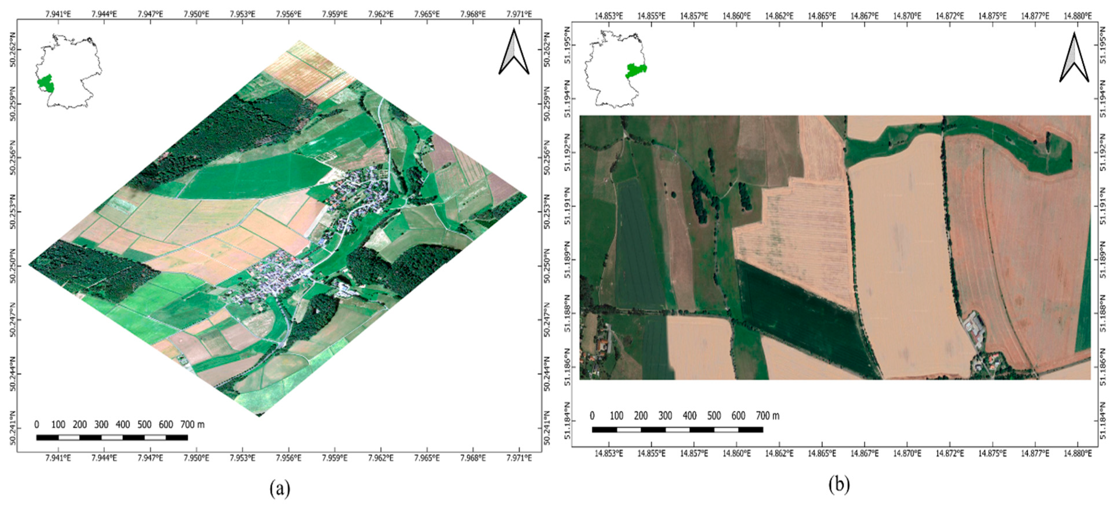
2.1. Study Area

Our study focuses on three villages in Germany: Königshain, Oberfischbach, and Mittelfischbach. These locations were selected based on both scientific and regulatory considerations, particularly altitude limitations for UAV operations.

Königshain, located in the state of Saxony near the city of Görlitz, was selected as the test site to evaluate model performance. Oberfischbach and Mittelfischbach, located in Rhineland-Palatinate and geographically close to each other, served as training sites for model development. This division allows for a rigorous assessment of the model’s generalization capabilities across different geographic regions. These areas were among the few where UAV flights could be legally conducted within the permitted altitude limits, ensuring compliance with regulatory guidelines while enabling high-resolution thermal data acquisition. Figure 1 provides a visual representation of the study areas.

2.2. Dataset

The dataset for this study includes data collected from three primary sources: the DJI Mavic 3T (manufactured by DJI, headquartered in Shenzhen, Guangdong, China) drone thermal images, Landsat-8, and Planet imagery, all collected between July and September 2024, as can be seen in

Table 1. Features extracted from multisource datasets.

Data Source	Type	Name	Resolution (m)	Simbol
DJI Mavic 3T drone	Thermal (High Resolution)	Temperature	0.23	THR
Landsat-8	Thermal (Low Resolution)	LST	30	LSTLR
PlanetScope	Surface Reflectance	Blue, Green, Red, and NIR	3	IHR
	Spectral Index	NDVI

and

Table 2. Meteorological conditions during each drone flight.

Date (UAV and Landsat-8)	Date (PlanetScope)	Site	Air Temperature (°C)	Humidity (%)	Air Pressure (hPa)
2024/07/29	2024/07/29	Oberfischbach	23	59.66	977.23
2024/08/17	2024/08/14	Konigshain	27	66.75	979
2024/09/07	2024/09/07	Oberfischbach	21.32	83	966
2024/09/07	2024/09/07	Mittelfischbach	22.66	75.33	967.7
-	2024/10/23	Mainz	-	-	-

.

The DJI Mavic 3T drones are equipped with state-of-the-art thermal and RGB cameras to capture high-resolution visual and thermal data in real time. The DJI Mavic 3T features a mechanical shutter, a 56× zoom camera, and an RTK module for centimeter-level precision, improving both mapping accuracy and operational efficiency (see

Table 3. Detailed specifications of DJI Mavic 3T adopted from (https://www.hammermissions.com/post/dji-mavic-3t-cameras-explained, accessed on 2 March 2023 and https://enterprise.dji.com/de/mavic-3-enterprise/specs, accessed on 24 July 2024).

Items	Camera Configuration	Detailed Specifications
DJI Mavic 3T	Camera configuration	Weight: 920 g Max. Flight Time: 45 min Max. Speed: 21 m/s Operating Temperature: −10 to 40 °C
Sample thermal image	Thermal camera	Sensor: Uncooled VOx Microbolometer Resolution: 640 × 512 pixels Spectral Range: 8–14 μm Accuracy: ±2 °C Field of View (FOV): 61° Focal Length: 40 mm
Sample RGB image	Telephoto Camera	Sensor: 1/2-inch CMOS Resolution: 4000 × 3000 pixels Field of View (FOV): 15° Focal Length: 162 mm
Sample RGB image	Wide Camera	Sensor: 1/2-inch CMOS Resolution: 8000 × 6000 pixels Field of View (FOV): 84° Focal Length: 24 mm

for more detail). Ideal for applications such as microclimate monitoring and precision agriculture, these drones provide precise temperature analysis in day and night conditions.

PlanetScope satellite imagery provides the highest spatial resolution among several satellite sensors, including Sentinel, Landsat, and MADIS, with a resolution of 3 to 5 m (resampled to 3 m). The collected data are pre-processed by ground stations and the MODIS sensor to remove atmospheric effects, allowing the use of ready-made products, including several types of basemaps for analysis [38]. These basemaps are divided into two types: Global and Select Basemaps (https://www.planet.com/products/basemap/, accessed on 24 July 2024).

Global basemaps cover the entire Earth’s surface, with special attention given to minimizing distortion in the polar regions. In contrast, Select Basemaps are created upon request for specific regions and can be produced at weekly, monthly, or seasonal intervals. Both types of basemaps include Visual Basemaps and Surface Reflectance Basemaps. Visual basemaps undergo atmospheric and color correction to improve image quality, while surface reflectance basemaps correct for atmospheric interference (https://www.planet.com/products/basemap/).

PlanetScope images are not publicly available but are available through subscription plans for academic institutions and research teams. These plans include the Basic Subscription for students and faculty, the Research Subscription for academic teams, and the Campus Subscription for campus-wide access. Depending on the subscription, users can download up to 100 million square kilometers of imagery per year, including both global and archived high-resolution SkySat data. This ensures that researchers have access to high-quality satellite data while benefiting from academic discounts (https://www.planet.com/industries/education-and-research/, accessed on 24 July 2024).

Equipped with OLI and TIRS sensors, Landsat 8 provides 30 m resolution multispectral imagery with global coverage every 16 days. Its reliable and consistent coverage mean that Landsat 8 is widely used in agriculture, natural resource management, and environmental monitoring [39].

Processing of Thermal Drone Images for Temperature Retrieval

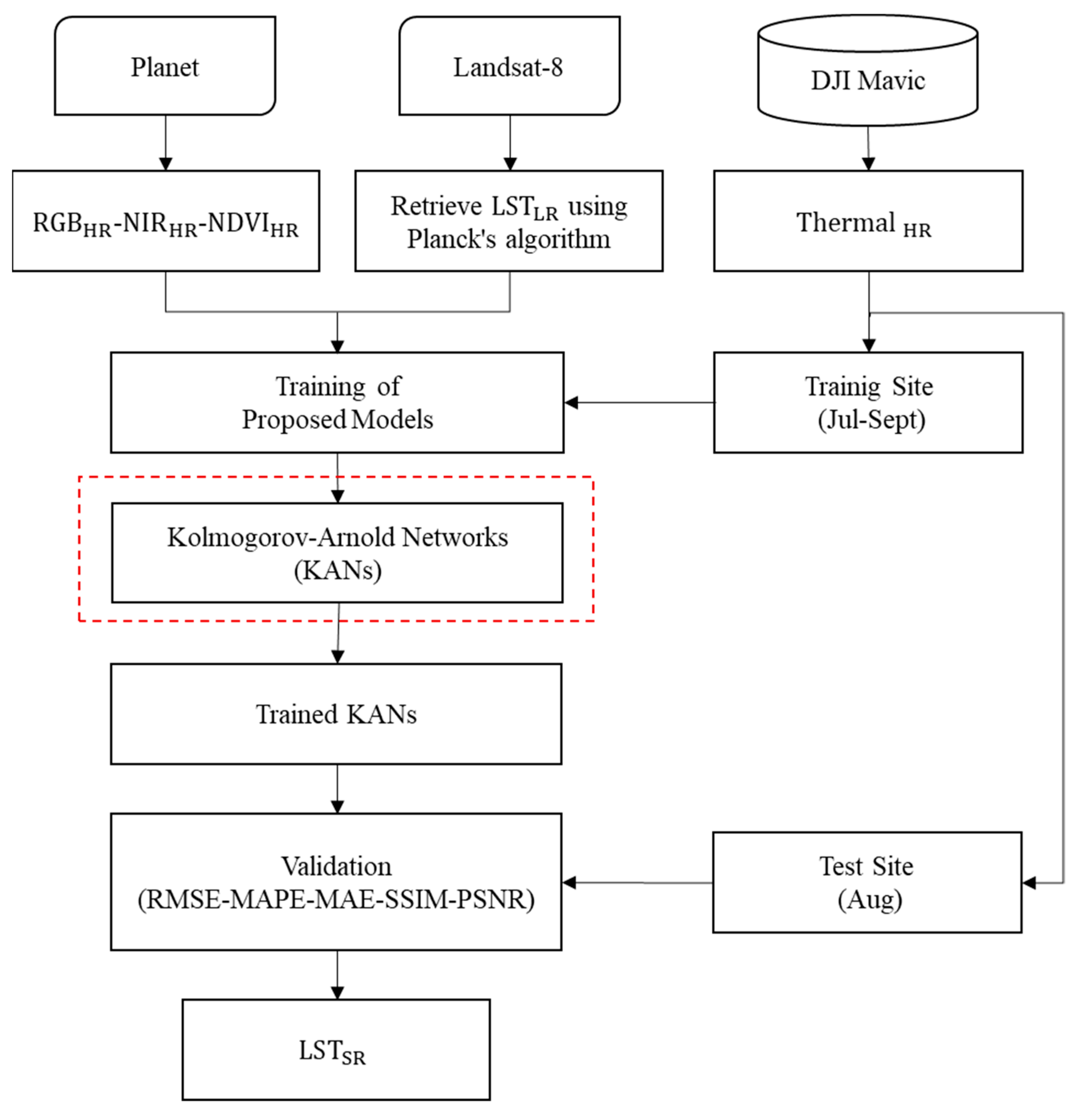
Drone-captured thermal images provide a basic thermal view of an area but do not directly yield absolute temperature data in TIFF format. To convert these raw images from a DJI Mavic 3T into absolute temperatures, a script using DJI Thermal SDK in R has been developed (available at https://github.com/DanGeospatial/dji_m3t_rpeg_to_tif, accessed on 29 January 2024 and https://www.dji.com/downloads/softwares/dji-thermal-sdk, accessed on 7 July 2024).

To ensure accurate conversion, it is crucial to calibrate parameters like emissivity, humidity, camera-to-target distance, and surface reflectance. The process begins with extracting metadata from the images using the exifr tool. The raw images are then calibrated using DJI Thermal SDK, converting them to absolute temperature values in Celsius in TIFF format. Finally, metadata including camera model and geographic location are added to the TIFF files. This detailed process creates data ready for use in geographic software like Agisoft Metashape (v2.0.1), enabling the production of thermal orthophotos with precise temperature values.

2.3. Methodology

The proposed method for super-resolution LST (LST_SR) in Germany involves a multi-step process, as fully illustrated in Figure 2.

First, T_HR images were collected using the DJI Mavic 3 Thermal drone. These images, with a spatial resolution of 23 cm, were acquired in July, August, and September 2024 to coincide with Landsat-8 satellite passes over the study area. This synchronization between drone and satellite data ensures that the images were acquired under similar environmental conditions. Simultaneously, I_HR images were collected from the Planet satellite. These I_HR were used to transfer spatial information from the optical images to the LST_LR. The transfer was performed either simultaneously with the drone data or with a time difference of one or two days to minimize significant changes in vegetation cover during the observation period. The T_HR images were first calibrated using the DJI Thermal SDK. A thermal ortho-photo was then generated using Agisoft software (v2.0.1). Additionally, LST_LR images were extracted from Landsat-8 using the Planck algorithm [40]. Spectral bands and the Normalized Difference Vegetation Index (NDVI) were extracted from the I_HR images, and for accurate alignment, all features were resampled to a resolution of 3 m using the nearest neighbor method. An affine transformation was applied to ensure accurate geographic positioning. Finally, the KAN model was trained using data from training sites and tested on a test site to assess its accuracy and effectiveness in generating LST_SR. A detailed exposition of the KAN model and comparison models is provided in Section 2.3.1 and Section 2.3.2.

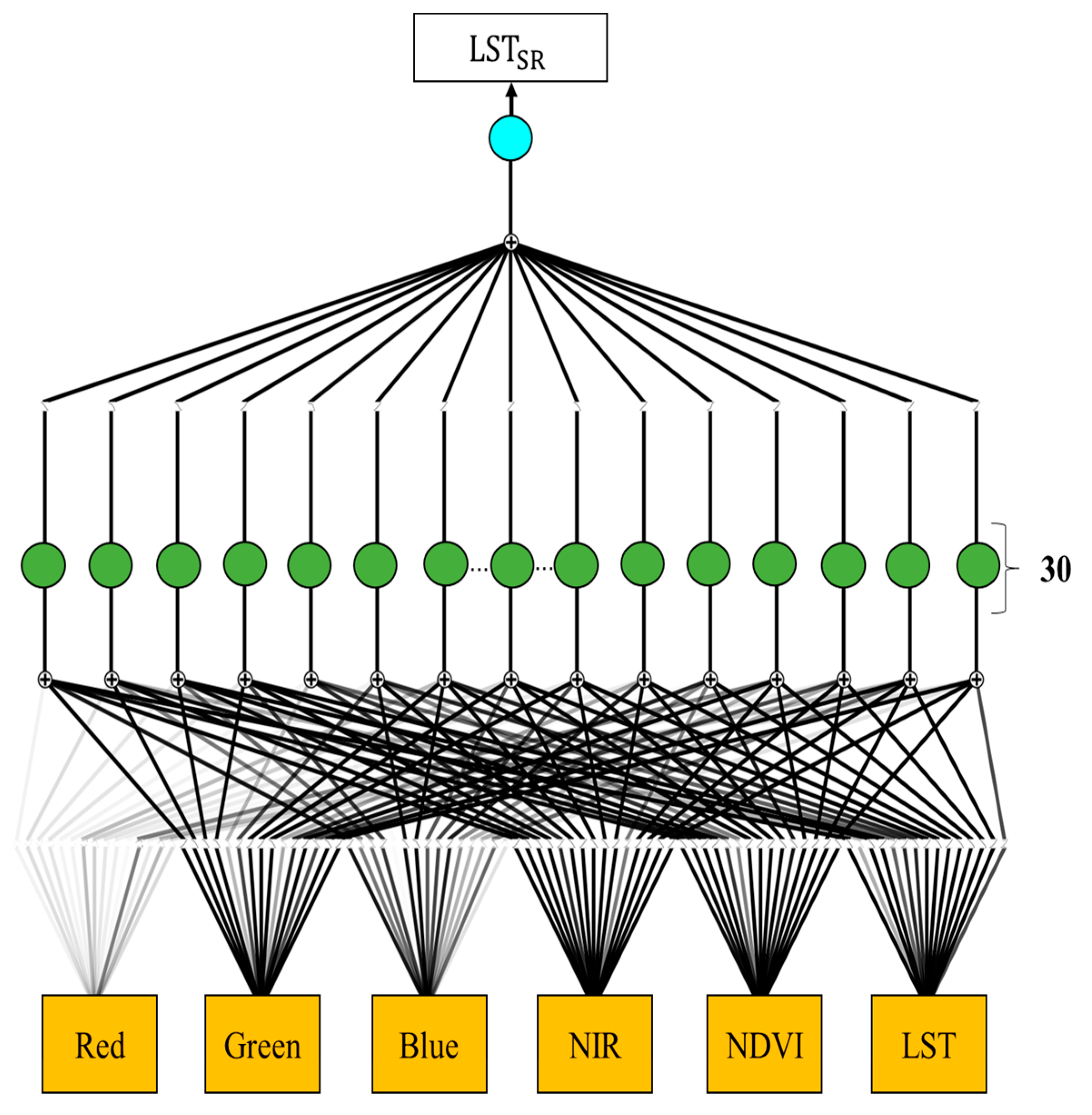
2.3.1. Kolmogorov–Arnold Network Architecture

To improve the resolution of LST, we propose the Kolmogorov–Arnold network (KAN) model, introduced by Liu [37]. The KAN, a dynamic deep learning architecture, addresses the limitations of traditional neural networks, particularly MLPs [41]. Unlike MLPs, which rely on fixed activation functions, the KAN model utilizes parameterized spline-based functions, eliminating dependence on fixed linear weights. This design significantly enhances the model’s flexibility and ability to capture precise boundaries and edges, resulting in improved performance and accuracy.

The KAN model employs a fully connected architecture, similar to MLPs, with nodes aggregating input features (see Figure 3). By integrating the advantages of splines and MLPs, the network achieves a robust capacity for learning at various depths, from shallow to deep layers, thus yielding significant results [37].

The KAN is based on the Cauchy–Kolmogorov theory, which states that any complex multivariate function can be decomposed into a combination of univariate functions and linear or nonlinear composites [42]. Leveraging this principle, the KAN combines the expressiveness of splines for univariate functions with the robust learning capabilities of deep networks for complex compositions. This hybrid approach enables the precise handling of high-dimensional inputs.

For example, in this model, the multivariate function ${LST}_{SR}$ is defined as follows:

$${LST}_{SR}=f(x_l)=f(B_{red},B_{green},B_{blue},B_{nir},B_{ndvi},{LST}_{LR})=\sum _{m=1}^{2l+1}{\Psi }_m(\sum _{n=1}^l{\psi }_{m,n}(x_n))$$

(1)

where $B_{red},B_{green},B_{blue},B_{nir},B_{ndvi},{and LST}_{LR}$ represent the input variables, $l$ is the number of variables, ${\Psi }_m$ is the learnable nonlinear functions responsible for processing and combining outputs of the univariate functions ${\psi }_{m,n}$, and ${\psi }_{m,n}$ is the parameterized spline-based univariate functions.

The input variables $B_{red},B_{green},B_{blue},B_{nir},B_{ndvi},{and LST}_{LR}$are passed directly to the univariate functions ${\psi }_{m,n}$. These functions process the input values to produce intermediate outputs:

$${z_{m,n}=\psi }_{m,n}\left(x_n\right),m\in \left\{1,\dots ,M\right\}, n\in \left\{1,\dots ,l\right\}$$

(2)

where $z_{m,n}$ represents the processed output of each univariate function. Splines are essential for capturing complex data features with high precision.

The outputs $z_{m,n}$ of the univariate functions are summed for each m to form an initial linear combination:

$$s^m=\sum _{n=1}^l{z}_{m,n}$$

(3)

The linear combinations $s^m$ are passed through the learnable nonlinear functions ${\Psi }_m$, which extract complex features from the input:

$$y^m={\Psi }_m(s^m)$$

(4)

Finally, the outputs of all ${\Psi }_m$ functions are combined to reconstruct the LST_SR:

$${LST}_{SR}=\sum _{m=1}^M{y}^m$$

(5)

Network parameters are initialized using Xavier initialization, while spline functions are initially set to approximate near-linear behavior. Training is performed using optimization algorithms such as LBFGS or Adam, ensuring faster convergence compared to traditional MLP methods. Fine-tuning the spline functions allows the model to capture intricate details in the data. Unlike MLPs that require additional nodes for higher accuracy, the KAN achieves superior performance with fewer parameters due to its learnable spline-based activation functions [37].

In addition, the KAN excels at handling complex data structures while mitigating overfitting through adaptive nonlinear activation functions. Unlike MLPs, which operate as black-box models, the KAN improves interpretability by allowing for direct examination of the learned activation functions. The initial results show that the KAN outperforms MLPs with fewer parameters, positioning it as a powerful tool for tasks like image processing and solving high-dimensional problems [37].

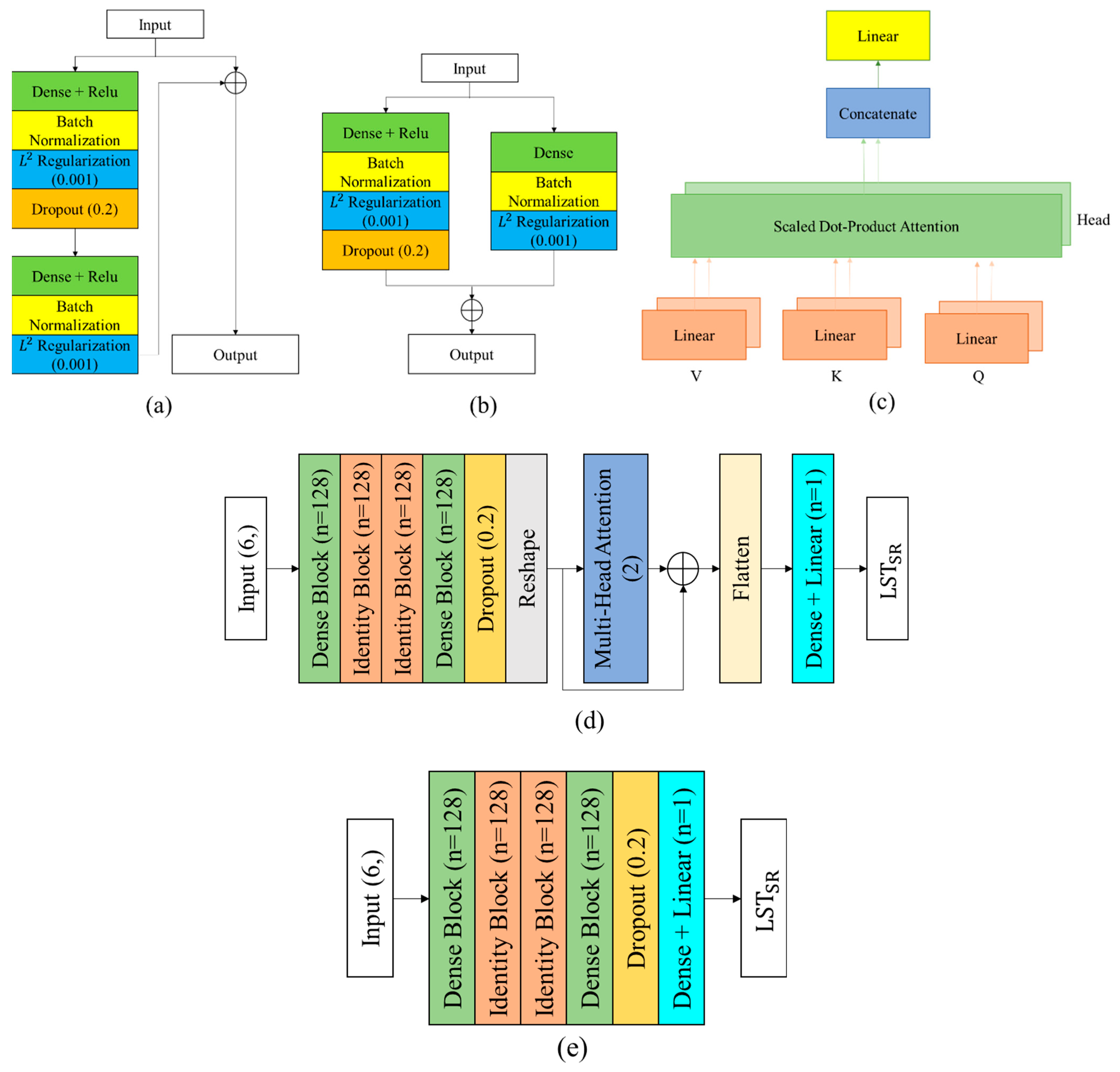
2.3.2. Comparison Models

We compared the KAN architecture with various ML/DL methods, including LightGBM, XGBoost, ResDenseNet, and ResDenseNet-Attention (Figure 4). The ResDenseNet-Attention architecture combines advanced DL components, including Dense Blocks, Identity Blocks, and the multi-head residual attention mechanism, to effectively extract and refine spatial and contextual features [43,44,45,46]. To design the ResDenseNet model, we removed the attention block from the ResDenseNet attention architecture. In the following text, the architecture of the ResDenseNet and its multi-head residual attention mechanism will be explored in detail.

ResDenseNet Architecture

The ResDenseNet architecture is a DL model that includes advanced components such as Dense Blocks and Identity Blocks [47].

The Dense Block ($B_D$) incorporates several main processes to enhance feature extraction and prevent overfitting. These include skip connections, activation functions, batch normalization, L²-regularization, and dropout, as described in Equations (6)–(8):

$$B_{D1}=D(ReLU(BN(L^2\left(w.x+b\right))))$$

(6)

$$B_{D2}=BN(L^2(w.B_I+b))$$

(7)

$$B_D=B_{D1}+B_{D2}$$

(8)

where $x$, $w$, $b$, $L^2$, $BN$, $ReLU$, and $D$ are the input, the weights of the dense layer, biases of the dense layer, $L^2$-regularization, batch normalization, activation function, and dropout. These blocks can robustly learn high-level features without overfitting the data.

The Identity Block ($B_I$) extracts high-level features from the input while preserving critical information through shortcut connections (Equations (9)–(11)):

$$B_I=D(ReLU(BN(L^2\left(w.B_D+b\right))))$$

(9)

$$B_I=ReLU(BN(L^2(w.B_I+b)))$$

(10)

$$B_I=B_I+B_D$$

(11)

Multi-Head Residual Attention Block

A main innovation in the ResDenseNet architecture is the multi-head residual attention block. This component captures intricate spatial and contextual relationships within the data, enabling the model to focus on fine-grained details. The attention mechanism computes scaled dot-product attention for multiple heads in parallel (Equations (12)–(15)) [43,46]:

$$Attention \left(Q.K.V\right)=Softmax \left({\displaystyle \frac{Q K^t}{\sqrt{d_K}}}\right)V$$

(12)

$$MHA=Linear (concat\left({Head}_1,{Head}_2\right))$$

(13)

$$MHRA=MHA+{Output}_{ResDensNet}$$

(14)

$${LST}_{SR}=Dense \left(MHRA\right)$$

(15)

The query ($Q$), key (K), and value (V) projections are computed from the output of the ResDenseNet (O_ResDenseNet) using learnable weight matrices W_Q, W_K, and W_V. Specifically,

Q = O_ResDenseNet·W_Q, K = O_ResDenseNet·W_K, V = O_ResDenseNet·W_V

(16)

The dimensionality of the key (d_K) is used to scale the dot-product attention scores, ensuring stable gradients during the softmax operation. This scaling prevents the softmax from becoming too sensitive to large input values, which could otherwise lead to numerical instability [43,46].

The outputs of all attention heads are concatenated and passed through a linear transformation layer to produce the final multi-head attention output. This mechanism enables the model to simultaneously focus on multiple spatial relationships within the data, effectively capturing fine-grained details and improving the overall accuracy of the LST_SR.

By integrating these components, ResDenseNet achieves highly accurate LST_SR, making it a powerful tool for precision applications in environmental monitoring, agriculture, and UHI.

LightGBM

The LightGBM model is a fast, memory-efficient decision tree algorithm that uses histogram-based techniques to bin continuous features, reducing training time and memory use [48]. Unlike traditional level-wise tree expansion, it adopts a leaf-wise growth strategy, prioritizing splits that minimize loss, leading to faster convergence and more accurate predictions. For further details, visit the official LightGBM documentation (https://lightgbm.readthedocs.io/, accessed on 4 May 2017) and original LightGBM paper [48].

XGBoost

XGBoost is a fast and powerful gradient-boosted decision tree algorithm known for its efficiency and accuracy [49]. It leverages techniques such as tunable learning rates, stochastic gradient boosting, and L1/L2 regularization to control complexity and prevent overfitting. With features like missing data handling, parallel tree construction, and incremental training, it optimizes both speed and scalability. Tree pruning removes insignificant nodes to enhance model efficiency, while built-in cross-validation ensures optimal boosting iterations for superior predictive performance. Additionally, its ability to handle large datasets and compatibility with distributed computing frameworks make it a preferred choice for various machine learning applications, including classification, regression, and ranking tasks. For more details, refer to the original XGBoost paper [49] and documentation: https://xgboost.readthedocs.io/, accessed on 21 July 2024.

2.3.3. Model Training and Experimental Setup

All experiments were performed using a Python (v3.11) script in Google Colaboratory (Colab) with GPU acceleration and 334 GB of RAM to optimize computational efficiency. The proposed model used six features derived from PlanetScope and Landsat-8 images as the input. Data from the villages of Oberfischbach and Mittelfischbach were used for training and evaluation. To ensure a balanced separation of training and validation samples, 30% of the training data were used for validation by sorting the ground truth data and extracting validation samples at fixed intervals. In addition, the Königshain region was used as a test dataset. The dataset consisted of 229,729 training pixels, 98,456 validation pixels, and 190,554 test pixels. To improve LST resolution, the Mainz dataset was used for SR_LST modeling, excluding UAV data. Training was performed using Mean Squared Error (MSE) as the loss function and with the Adam optimizer for efficient convergence. To improve model accuracy and prevent overfitting, the model’s hyperparameters were optimized by grid search. These hyperparameters included a learning rate of 0.05, which controls the step size of weight updates during training. Additionally, a dropout rate of 0.2 was used to prevent overfitting by randomly deactivating 20% of the neurons in each training step. Furthermore, L² regularization was applied with a value of 0.001 to reduce excessive weights and prevent model complexity. The number of neurons in the hidden layers of the KAN model was set to 30, and the number of filters per block was set to 128 in the ResDensNet model, which helps to improve feature extraction. The number of heads in the multi-head attention mechanism was set to two, allowing the model to focus on different parts of the input data simultaneously. The XGBoost and LightGBM models used 100 and 120 estimators (decision trees), respectively. These parameters helped to optimize the training process and improve the prediction accuracy of the model.

2.4. Evaluation Metrics

The performance of the proposed DL model and other comparative models in this study was evaluated using several metrics such as Root Mean Squared Error (RMSE), Mean Absolute Error (MAE), Mean Absolute Percentage Error (MAPE), Peak Signal to Noise Ratio (PSNR), Structural Similarity Index Measure (SSIM), and coefficient of determination (R²), which can be calculated using the following equations in

Table 4. Evaluation metrics for LST Super-Resolution performance.

Metric	Formula	Description	Ref
$\mathrm{R}\mathrm{M}\mathrm{S}\mathrm{E}$	$\sqrt{{\displaystyle \sum _{i=1}^N}{\displaystyle \frac{{(y_{{\mathrm{L}\mathrm{S}\mathrm{T}}_{\mathrm{S}\mathrm{R}}}^i-y_{{\mathrm{T}}_{\mathrm{H}\mathrm{R}}}^i)}^2}{N}}}$	Measures error magnitude, penalizing large errors.	[50]
$\mathrm{M}\mathrm{A}\mathrm{E}$	${\displaystyle \frac{1}{N}}{\displaystyle \sum _{i=1}^N}{y}_{{\mathrm{L}\mathrm{S}\mathrm{T}}_{\mathrm{S}\mathrm{R}}}^i-y_{{\mathrm{T}}_{\mathrm{H}\mathrm{R}}}^i$	Measures the average absolute difference between predicted and actual values, indicating model accuracy.	[51]
$\mathrm{M}\mathrm{A}\mathrm{P}\mathrm{E}$	${\displaystyle \frac{1}{N}}{\displaystyle \sum _{i=1}^N}{\displaystyle \frac{\left|y_{{\mathrm{L}\mathrm{S}\mathrm{T}}_{\mathrm{S}\mathrm{R}}}^i-y_{{\mathrm{T}}_{\mathrm{H}\mathrm{R}}}^i\right|}{y_{{\mathrm{T}}_{\mathrm{H}\mathrm{R}}}^i}}$	Calculates the relative error as a percentage, allowing easy comparison of models across different data scales.	[51]
$\mathrm{P}\mathrm{S}\mathrm{N}\mathrm{R}$	$20 {\log }_{10}({\displaystyle \frac{{max}_{{\mathrm{T}}_{\mathrm{H}\mathrm{R}}}-1}{RMSE}})$	Evaluates image prediction quality, with higher values indicating better quality.	[52]
$\mathrm{S}\mathrm{S}\mathrm{I}\mathrm{M}$	${\displaystyle \frac{\left(2{\mu }_{{\mathrm{L}\mathrm{S}\mathrm{T}}_{\mathrm{S}\mathrm{R}}}{\mu }_{{\mathrm{T}}_{\mathrm{H}\mathrm{R}}}+C_1\right)\left(2{\sigma }_{{\mathrm{L}\mathrm{S}\mathrm{T}}_{\mathrm{S}\mathrm{R}} {\mathrm{T}}_{\mathrm{H}\mathrm{R}}}+C_2\right)}{\left({\mu }_{{\mathrm{L}\mathrm{S}\mathrm{T}}_{\mathrm{S}\mathrm{R}}}^2+{\mu }_{{\mathrm{T}}_{\mathrm{H}\mathrm{R}}}^2+C_1\right)\left({\sigma }_{{\mathrm{L}\mathrm{S}\mathrm{T}}_{\mathrm{S}\mathrm{R}}}^2+{\sigma }_{{\mathrm{T}}_{\mathrm{H}\mathrm{R}}}^2+C_2\right)}}$	Assesses perceived image quality, considering luminance, contrast, and texture.	[50]
R2	$1-{\displaystyle \frac{\sum _{i=1}^N{(y_{{\mathrm{L}\mathrm{S}\mathrm{T}}_{\mathrm{S}\mathrm{R}}}^i-y_{{\mathrm{T}}_{\mathrm{H}\mathrm{R}}}^i)}^2}{\sum _{i=1}^N{(y_{{\mathrm{T}}_{\mathrm{H}\mathrm{R}}}^i-y_{mean})}^2}}$	Measures how well predictions match observations; closer to 1 means better fit.	[46]

Where N is the number of test samples, $y_{{\mathrm{T}}_{\mathrm{H}\mathrm{R}}}^i$ and $y_{{\mathrm{L}\mathrm{S}\mathrm{T}}_{\mathrm{S}\mathrm{R}}}^i$represent the observed thermal values and generated LST_SR values for the test samples, respectively, ${max}_{{\mathrm{T}}_{\mathrm{H}\mathrm{R}}}$ indicates the max of the observed thermal data, $y_{mean}$ indicates the average of the observed thermal data, ${\mu }_{{\mathrm{L}\mathrm{S}\mathrm{T}}_{\mathrm{S}\mathrm{R}}}$ and ${\mu }_{{\mathrm{T}}_{\mathrm{H}\mathrm{R}}}$ indicate the mean intensity of LST_SR generated and observed thermal values, ${\sigma }_{{\mathrm{L}\mathrm{S}\mathrm{T}}_{\mathrm{S}\mathrm{R}} {\mathrm{T}}_{\mathrm{H}\mathrm{R}}}$ indicates covariance between LST_SR generated and observed thermal values, ${\mu }_{{\mathrm{L}\mathrm{S}\mathrm{T}}_{\mathrm{S}\mathrm{R}}}^2$ and ${\mu }_{{\mathrm{T}}_{\mathrm{H}\mathrm{R}}}^2$ are variances of LST_SR generated and observed thermal values, and $C_1$, and $C_2$ are small constants to stabilize the formula, avoiding division by zero.

.

3. Result

The performance of the KAN model for the super-resolution of LST was evaluated in comparison with other traditional ML/DL methods, such as LightGBM, XGBoost, ResDensNet, and ResDensNet-Attention. The comparative results of the methods are shown in

Table 5. Comparison of performance between the KAN and other models for super-resolution of LST at the test site.

Model	RMSE (°C)	MAE (°C)	MAPE (%)	PSNR	SSIM	R2
LightGBM	6.17	5.36	16.68	18.58	0.76	−0.48
XGBOOST	5.45	4.72	14.79	19.66	0.70	−0.15
ResDensNet	6.42	5.80	18.41	18.18	0.78	−0.62
ResDensNet-Attention	4.74	4.08	12.72	20.87	0.81	0.12
KAN	4.06	3.09	9.32	22.22	0.83	0.35

for the evaluation metrics.

As shown in Table 5, the performance of the proposed model compared with other methods for generating LST_SR at the test site shows significant differences, highlighting the superior performance of the KAN model. In the experiments conducted for August, models such as ResDensNet, XGBoost, and LightGBM achieved RMSE values between 5.45 and 6.42, MAE values between 4.72 and 5.80, SSIM values between 0.70 and 0.78, MAPE values between 14.79 and 18.41, and PSNR values between 18.18 and 19.66. In contrast, advanced DL models showed significantly better performance. Among them, the KAN model was found to be the best, with an RMSE of 4.06, MAE of 3.09, MAPE of 9.32, SSIM of 0.83, and PSNR of 22.22. The ResDensNet-Attention model ranked second with an RMSE of 4.74, MAE of 4.08, MAPE of 12.72, SSIM of 0.81, and PSNR of 20.87. The KAN model showed significant improvements over the other models on metrics. It reduced the RMSE by about 14.34%, MAE by 24.26%, and MAPE by 26.73% compared to the previous best model (ResDensNet-Attention), while increasing PSNR by 6.47% and SSIM by 2.47%. In addition, compared to traditional models such as LightGBM and XGBoost, it reduced the RMSE by approximately 34.21% and 25.50%, and the MAPE by 44.15% and 36.98%, respectively. These results clearly confirm the superiority of the KAN model in capturing complex patterns in LST_SR. In addition, the KAN model achieved an R² value of 0.35, demonstrating its exceptional ability to explain and predict LST_SR variations with high accuracy. In contrast, the other models showed weaker performance in this respect. Specifically, LightGBM achieved an R² of −0.48 and XGBoost showed an R² of −0.15, both indicating their inability to effectively capture the underlying patterns in the LST_SR data. The ResDensNet-Attention model performed slightly better with an R² of 0.12 but still fell short of the KAN model. Not only did the KAN model outperform the other methods in terms of critical performance metrics such as RMSE, MAE, MAPE, PSNR, and SSIM, it also had a significantly higher R², highlighting its superior ability to model the complex relationships and trends essential in the LST_SR.

3.1. Evaluation of KAN Model Performance Using PlanetScope and Landsat-8 Imagery Combinations

To investigate the effect of different combinations of input features on the performance of the KAN model in generating LST_SR, a comprehensive evaluation was performed using multi-source satellite data from PlanetScope and Landsat-8 (

Table 6. Assessment of KAN model accuracy using combined PlanetScope and Landsat-8 imagery.

Planet			Landsat-8	Evaluation Metrics
RGB	NIR	NDVI	LST	RMSE (°C)	MAE (°C)	MAPE (%)	PSNR	SSIM
✓				5.93	4.86	14.27	18.92	0.82
✓	✓			4.92	3.96	12.18	20.55	0.82
✓	✓	✓		4.56	3.67	11.58	21.21	0.82
✓	✓	✓	✓	4.06	3.09	9.32	22.22	0.83
	✓	✓	✓	5.43	4.40	13.32	19.69	0.80
✓			✓	4.81	3.89	11.52	20.73	0.82

). The results showed that the simultaneous use of spectral bands (RGB and NIR), vegetation index (NDVI), and LST resulted in the highest reconstruction accuracy. Specifically, the RMSE decreased from 5.93 (RGB only) to 4.00, an improvement of 32.6%. Similarly, MAE and MAPE were reduced by 36.4% and 34.7%, respectively, while SSIM improved by 1.2%. In addition, the PSNR increased from 18.92 to 22.22, representing a 17.4% improvement in signal-to-noise ratio. These results clearly demonstrate the critical role of integrating complementary and multi-source inputs to improve model accuracy, reduce errors, and enhance the reconstruction of thermal surface patterns. Thus, the effective combination of surface reflectance, thermal, and vegetation features can be considered a key strategy for improving the performance of DL models in super-resolution LST.

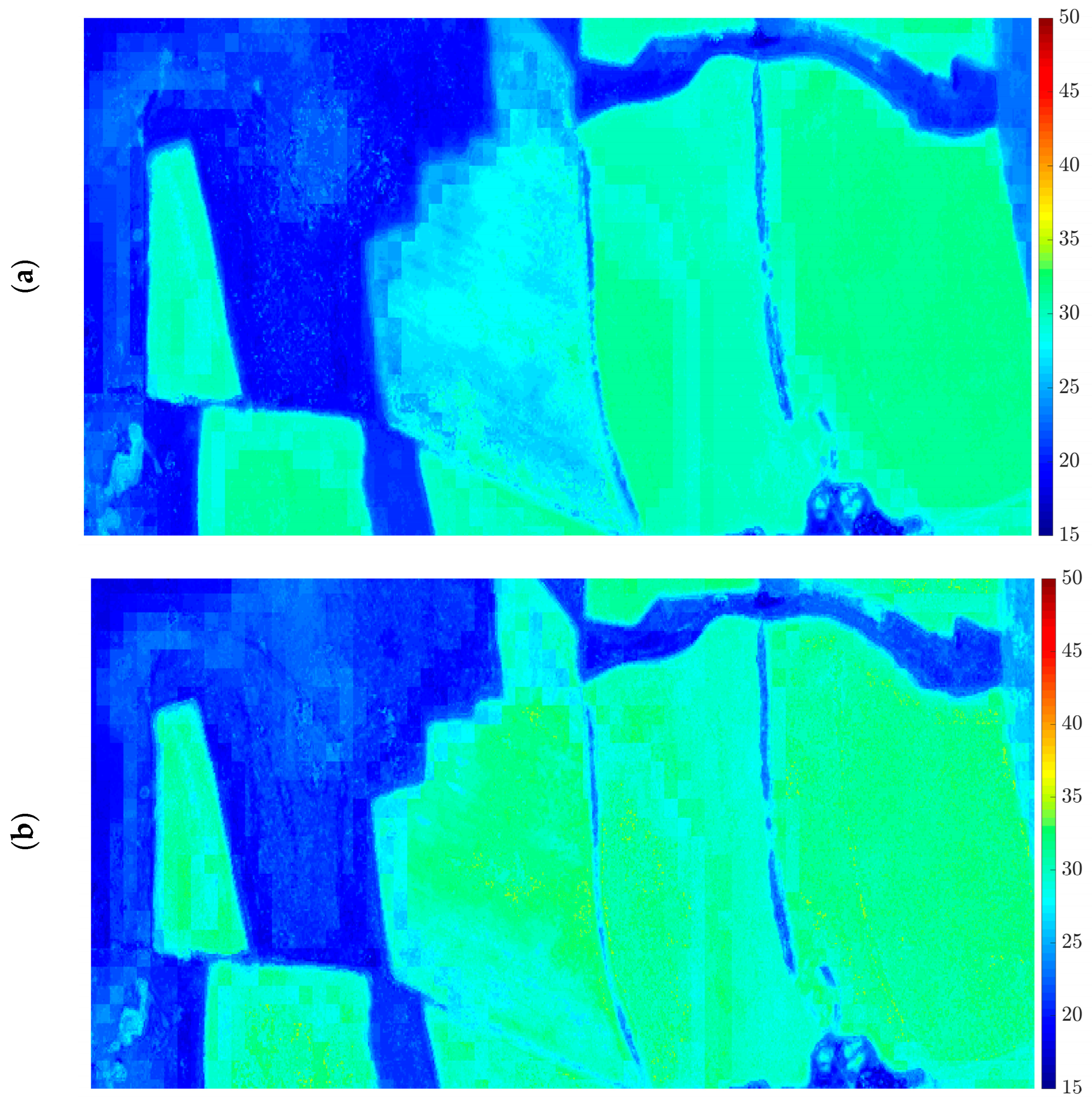
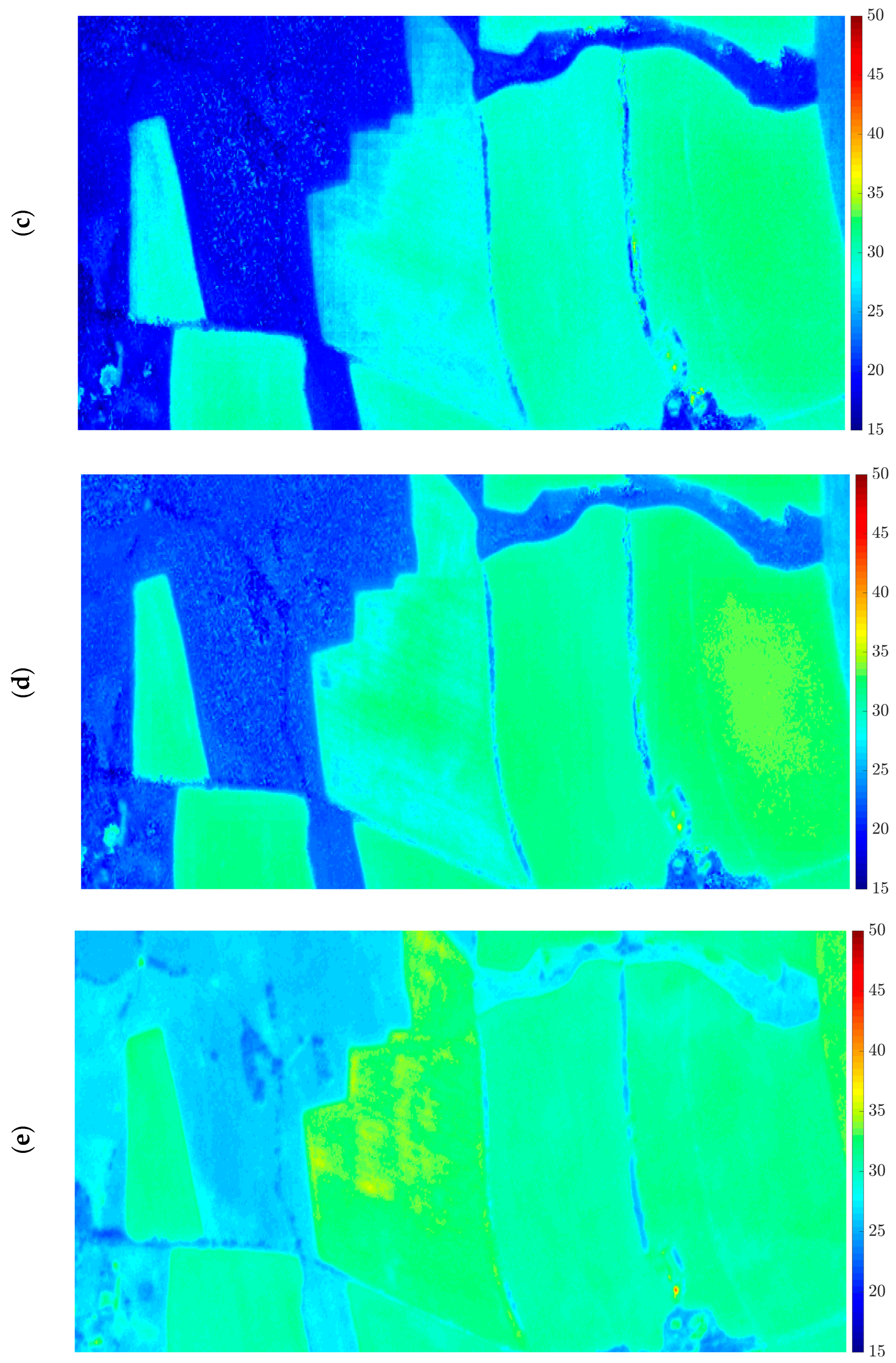
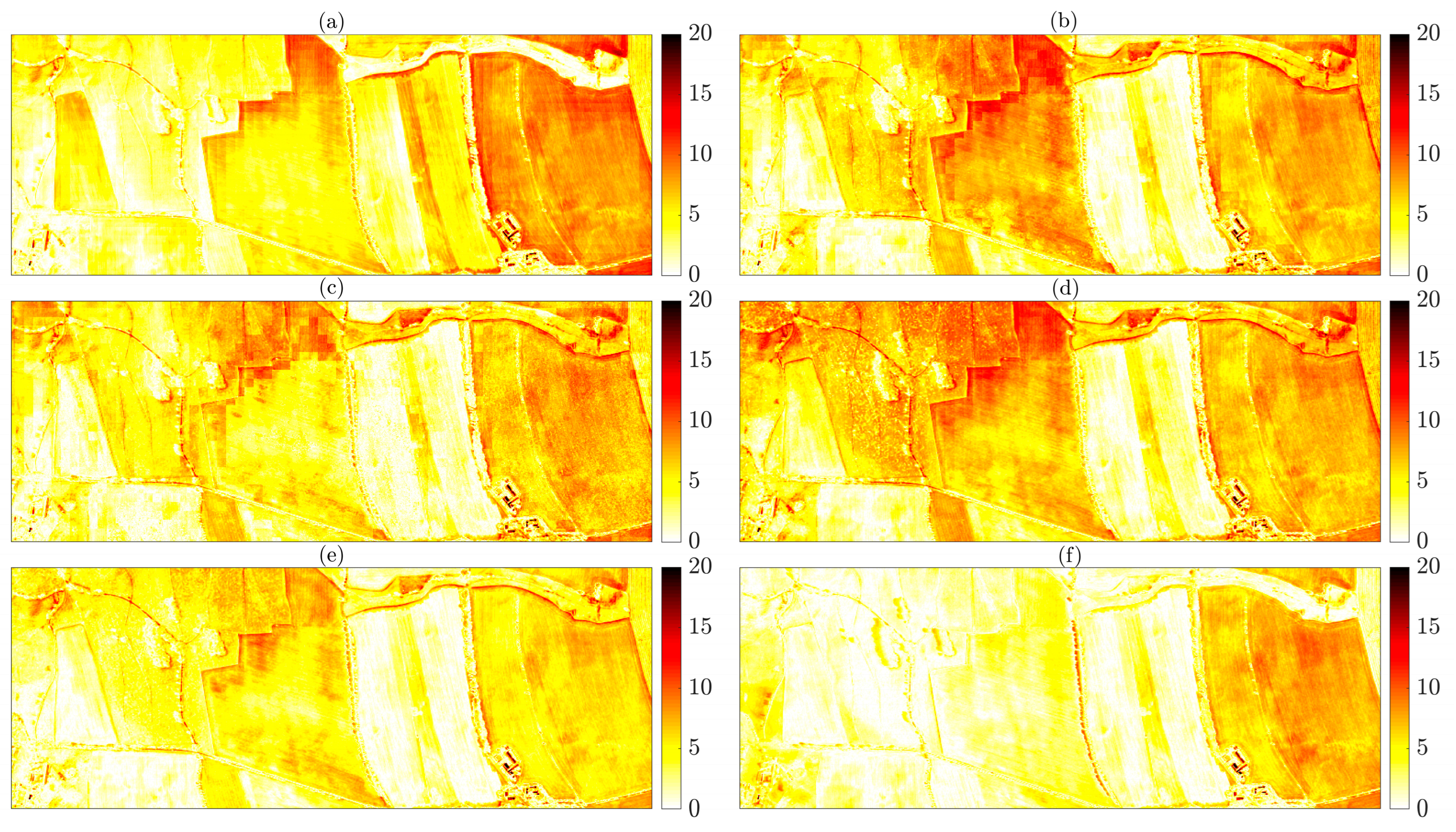
3.2. Visual Comparison

To visually evaluate the performance of the models, Figure 5 shows the reconstruction of the LST_SR by different models compared to the reference data (T_HR). In this analysis, the accuracy of the proposed and baseline models was evaluated using T_HR as reference data. As shown in Figure 5, advanced models such as ResDensNet-Attention and KAN successfully reconstruct the thermal structure with more detail and show better agreement with the reference data. Among them, KAN shows the best performance, particularly in preserving thermal boundaries, distinguishing between hot and cold regions, and accurately capturing fine-scale thermal variations. In contrast, traditional models such as LightGBM and XGBoost are less accurate in simulating thermal details, producing outputs that appear overly smoothed and lack subtle thermal variations. This weakness highlights the limitations of traditional approaches in reconstructing complex thermal patterns and effectively capturing temperature dynamics.

From a visual accuracy perspective, both KAN and ResDensNet-Attention clearly outperform the other models. Not only do they reconstruct thermal variations with greater clarity, but they also simulate thermal structures with greater precision. These results highlight the superiority of DL-based models over traditional methods and confirm that KAN and ResDensNet-Attention are more suitable for advanced applications requiring high accuracy in the analysis of thermal patterns.

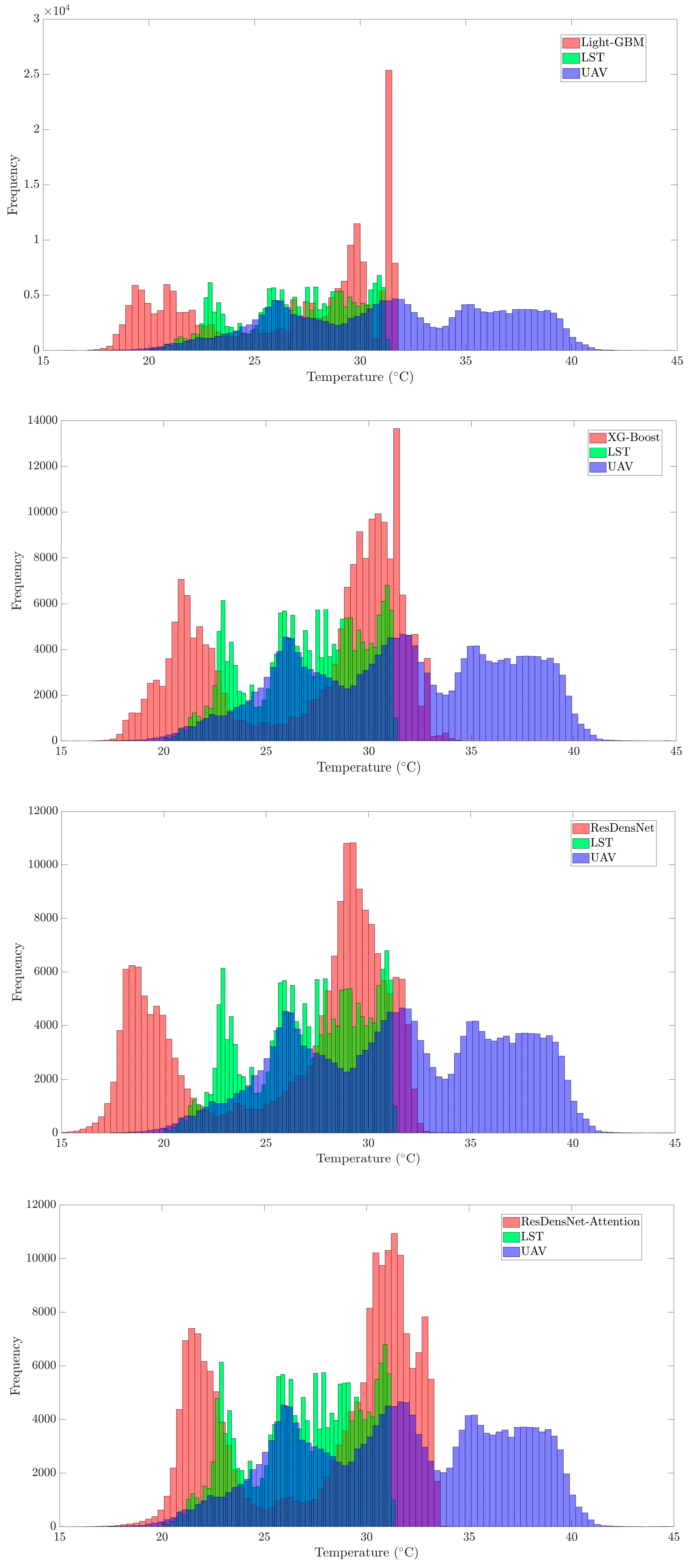
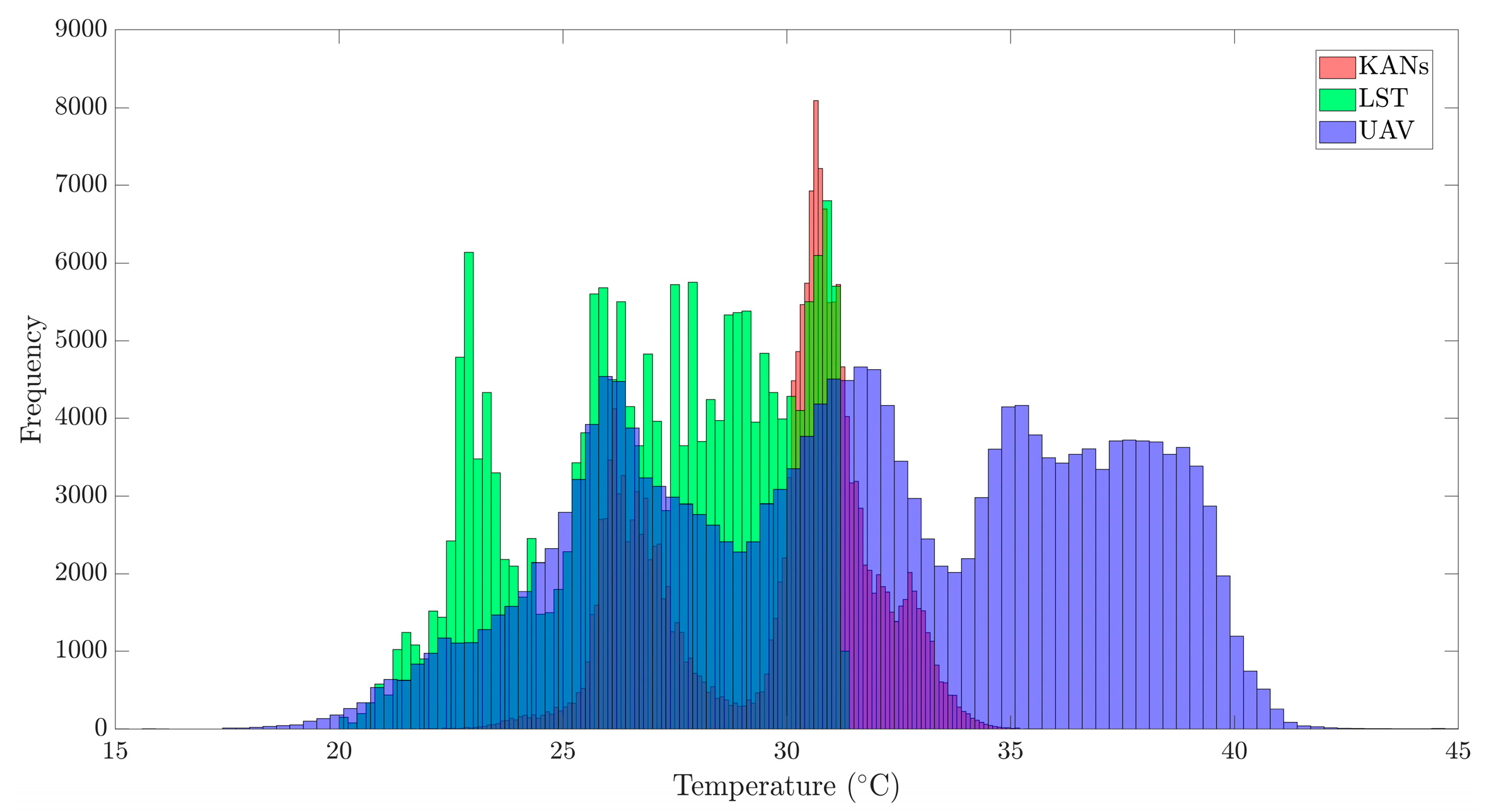
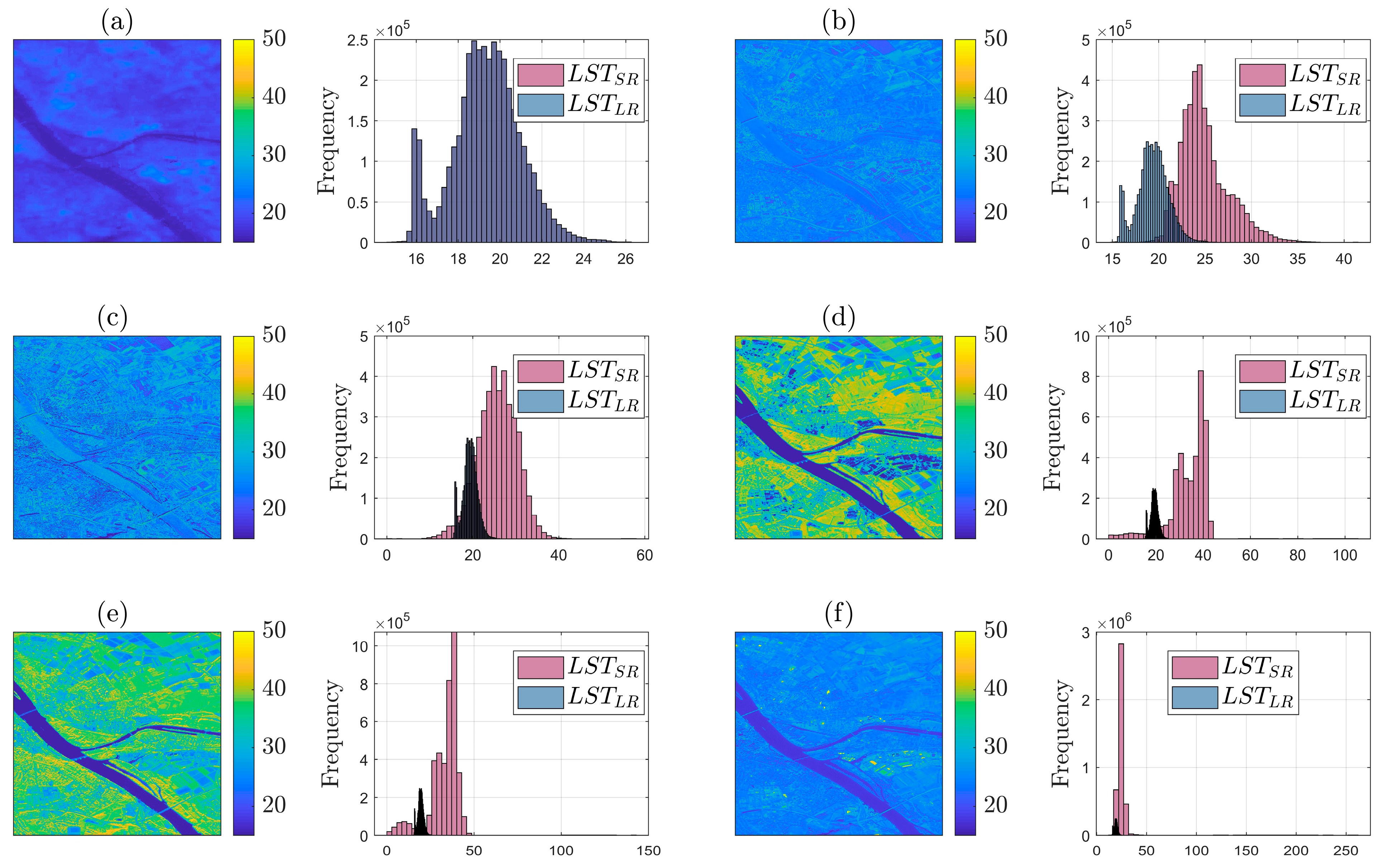
3.3. Histogram and Distribution Analysis

Figure 6 shows histograms illustrating the distribution of LST for both the proposed and baseline models, including LightGBM, XGBoost, ResDensNet, ResDensNet-Attention, and KAN, compared to T_HR and LST_LR observations. The histogram of T_HR (blue) serves as a more accurate and reliable reference for evaluating model performance. Traditional models, such as LightGBM and XGBoost, have limitations in capturing the true temperature distribution, as indicated by the lower overlap of their output histograms (red) with the T_HR and LST_LR (green). In contrast, the advanced models such as ResDensNet and ResDensNet-Attention show improved reconstruction accuracy, with better agreement with the T_HR. Of all the models, the KAN provides the most accurate results, effectively reconstructing both the peaks and the overall temperature distribution. Its histogram shows the highest degree of similarity to T_HR, reflecting strong consistency and the precise capture of finer temperature variations and complex thermal patterns. Overall, the KAN outperforms all other models in terms of reconstruction accuracy and agreement, with the T_HR confirming its robustness and effectiveness in modeling LST_SR distributions.

3.4. Error Map Evaluation

Figure 7 shows the LST_SR error maps generated by different models compared to the T_HR at the test site. These maps clearly show the spatial distribution of the reconstruction errors over the area. The results show that models based on advanced DL architectures exhibit more optimized and uniform error distributions compared to traditional ML models, highlighting the superior performance of DL models in LST_SR tasks.

Among the evaluated models, the KAN approach stands out by providing the most accurate and clearest error map. It effectively reduces errors and shows a higher degree of alignment with the T_HR.

In particular, most of the errors are concentrated in areas with buildings and man-made structures, which tend to have high temperatures. The high reflectivity, surface heterogeneity, and thermal complexity in these regions make accurate temperature reconstruction difficult.

This pattern indicates that despite the thermal complexity of urban and rural areas, the KAN model performs exceptionally well in reducing errors and providing more accurate temperature reconstructions. Thus, the KAN outperforms other models in temperature reconstruction, making it a strong choice for advanced LST pattern reconstruction applications.

3.5. Profile Comparisons

Figure 8 shows two comparative profiles of the generated LST_SR over the diagonal and anti-diagonal pixels, used to evaluate the performance of the different models. The LST_LR profile shows smoother temperature variations with less variability and limited detail, while the T_HR profile shows greater variability and finer detail. LST_SR generated by DL models such as KAN, ResDensNet, and ResDensNet-Attention are more similar to T_HR, while traditional models such as XGBoost and LightGBM show less effective performance. Generally, the KAN model stands out as the most accurate, providing predictions that are better aligned with the T_HR.

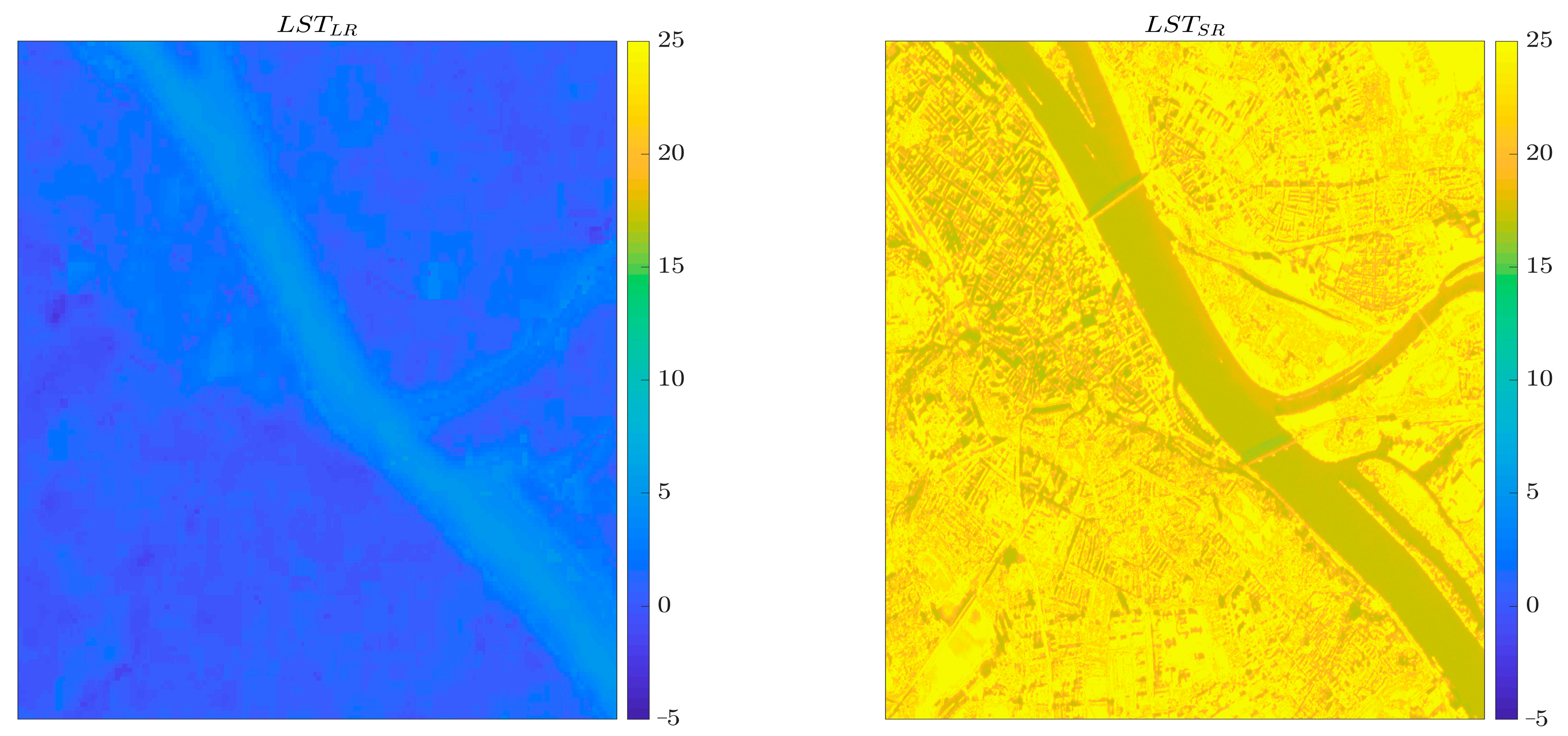
3.6. Generating the LST_SR Using Different Models in Mainz, Germany

In this study, for further analysis, the trained KAN model was applied to PlanetScope and Landsat-8 imagery to generate the LST_SR map for the city of Mainz, in the state of Rhineland-Palatinate, Germany, on 23 October 2024 (Figure 9). As shown in Figure 10, the proposed and comparison models were used to generate LST_SR maps using LST data from Landsat-8 and PlanetScope imagery.

Each model demonstrated different levels of accuracy in temperature reconstruction, highlighting the strengths and weaknesses of the different methods. The LST_LR map derived from Landsat-8 imagery had low spatial resolution and limited detail. In this map, various surface features appeared uniform, making it difficult to distinguish between urban, agricultural, and natural areas. While this map provided an overall view of LST, it was unable to show subtle temperature differences between regions.

In contrast, ML models such as LightGBM and XGBoost have a better ability to extract features and generate more accurate temperature maps. However, these models often introduce significant noise due to their reliance on high-level extracted features. This results in spatial inconsistencies and unrealistic temperature differences, making the maps generated less reliable. While these models can simulate general temperature patterns, they may generate unrealistic estimates in some areas due to overfitting or insufficient feature generalization.

DL models, such as ResDensNet and ResDensNet-Attention, offer higher accuracy in reconstructing structural details and provide better spatial resolution. However, these models typically overestimate LST, resulting in overstated temperature differences between regions. This can lead to errors in environmental and urban analyses. The ResDensNet-Attention model, which uses an attention mechanism, increases the resolution of temperature transitions but still suffers from overfitting, resulting in lower accuracy for accurate temperature mapping.

Of all the models evaluated, KAN provides the best balance between spatial resolution and temperature estimation accuracy. Unlike other models, KAN is able to reconstruct temperature variations realistically and reliably. This model preserves high-resolution detail and prevents overfitting, resulting in a more natural representation of thermal patterns.

Key advantages of the KAN model include its ability to accurately reconstruct features such as water bodies, roads, and agricultural areas with minimal noise. It offers high spatial resolution and provides more realistic temperature estimates than other models. In addition, KAN can distinguish temperature differences without creating exaggerated contrasts and retains structural details for a natural and reliable representation of temperature variations.

These results highlight KAN’s superior performance in producing highly accurate LST_SR maps with spatial consistency and stability. Given these advantages, KAN has become a highly effective tool for urban climate studies, agricultural monitoring, and environmental research, providing reliable insights for various Earth observation applications.

Comparing LST_SR Using Different Models to LST Landsat-8

Due to the limited availability of high-resolution LST reference data for the study area (city of Mainz), direct evaluation of LST_SR accuracy against high-resolution reference data was not possible. Therefore, the Landsat-8 derived LST map was used as a reference to compare model performance. According to previous studies, the RMSE difference between LST derived from UAV thermal imagery and Landsat-8 LST is reported to be 5 °C [53]. This predicted discrepancy was also observed in our results, confirming the validity of the KAN model output, which shows that its LST_SR temperature is approximately 5 °C higher than the Landsat-8 LST [53].

As shown in

Table 7. Performance comparison of LST_SR generated using different models based on Landsat-8 imagery.

Model	RMSE (°C)	MAE (°C)	Correlation
LightGBM	6.21	5.66	0.27
XGBoost	7.87	6.79	0.08
ResDensNet	17.46	16.10	0.25
ResDensNet-Attention	15.95	14.72	0.23
KAN	5.75	4.98	0.55

, the KAN model achieved the lowest RMSE (5.75) and MAE (4.98) values among all models, with the highest correlation coefficient (0.55) with the Landsat-8 data. These values indicate a closer agreement with the LST_LR compared to other models. In contrast, the ResDensNet and ResDensNet-Attention models had higher error values (RMSE of 17.46 and 15.95, respectively) and lower correlation coefficients (0.25 and 0.23), while they may generate sharper visual outputs.

In addition,

Table 8. Comparative analysis of statistical metrics for LST_SR generated by different models.

Model	Mean (°C)	Median (°C)	Std
Landsat-8	19.32	19.37	1.69
LightGBM	24.92	24.45	2.60
XGBoost	25.63	25.75	4.54
ResDensNet	30.72	35.20	13.57
ResDensNet-Attention	32.93	36.26	8.57
KAN	24.28	24.54	3.48

shows that the mean, median, and standard deviation (Std) of the KAN model’s LST_SR output are more consistent with LST_LR, given the predicted 5 °C difference. For example, while the Landsat-8 mean temperature is 19.32 °C, the KAN model estimates a mean temperature of 24.28 °C with a Std of 3.48, compared to much higher values produced by ResDensNet-Attention (mean = 32.93 °C, Std = 5.57). Therefore, although the output of the KAN model may appear visually smoother, statistical evaluation clearly shows that this model provides more accurate and reliable temperature estimates within the available data framework.

4. Discussion

4.1. LST and Its Importance

Accurate LST data at finer spatial scales are essential for several applications, particularly in UHI studies, agriculture, and climate change research. Urbanization amplifies UHI effects due to reduced green spaces, making LST maps crucial for identifying hotspots and informing interventions like green roofs and cool pavements [54]. In agriculture, accurate LST data optimize crop management, help monitor crop performance, and assess crop stress, thus improving irrigation practices and water resource use [55]. In addition, LST is essential for studying the effects of global warming, monitoring climate change, and understanding the relationship between land use patterns and temperature [56,57,58,59]. Research has shown a negative correlation between temperature and vegetation cover, and a positive correlation between temperature and built-up areas or bare soil, providing valuable insights for sustainable urban planning and climate change mitigation [58,59].

4.2. Challenges in LST Data Accuracy

While LST data are essential, several challenges affect their accuracy. The type of land use land cover (LULC) has a significant impact on the accuracy of generated LST maps. LULC such as bare land, agricultural areas, and forests have different emissivity properties that can introduce errors when estimating LST at finer scales [60]. Factors such as albedo, optical properties, and atmospheric conditions such as cloud cover, aerosols, humidity, and meteorological factors (e.g., wind, precipitation) can contribute to errors ranging from 0.2 °C to 0.7 °C [9]. These errors are particularly pronounced in mountainous or snow-covered regions, further complicating temperature estimation. In addition, surface emissivity, which can introduce errors in the range of 0.2 °C to 0.4 °C, is a significant source of uncertainty in LST data [9]. A comprehensive understanding and analysis of these factors, along with incorporating diverse land use and land cover (LULC) types and considering various regions and seasons in the training data, can significantly enhance the generation of high-resolution LST data.

4.3. Technological Impact on LST Accuracy

The significant difference in thermal image quality between drones and satellite-based platforms such as Landsat 8 further highlights the importance of high spatial resolution. Drone-based thermal imagery provides more detailed, higher-resolution data, allowing for better temperature measurements due to superior sensor accuracy and sensitivity. Drones operate at lower altitudes and capture images under favorable atmospheric conditions, reducing the impact of clouds and other weather factors that can affect satellite imagery. In contrast, Landsat 8 provides broader coverage at a lower spatial resolution (30 m), which results in a loss of detail. As a result, drone-derived LST data tend to be more accurate, as evidenced by studies showing a higher coefficient of determination (R²) between drone LST data and field measurements (0.89) compared to Landsat 8 (0.70) [61]. Higher resolution data, especially from drones, enable more accurate and localized temperature mapping, which is critical for urban planners looking to identify areas vulnerable to heat stress, or farmers looking to optimize irrigation practices. The enhanced detail allows for more tailored interventions and more effective policy strategies.

4.4. Downscaling LST Data

Several key factors are instrumental in the success of the LST downscaling process, with model selection and input data quality being the most critical. In this study, the KAN model demonstrates significant superiority over alternative methods, such as LightGBM and XGBoost, due to its exceptional capability to simulate complex temperature patterns and accurately reconstruct spatial details. By leveraging parametric splines, the KAN model effectively captures thermal structures, ensuring the preservation of temperature’s physical properties at finer scales.

One of the primary challenges in LST downscaling is the loss of spatial accuracy, particularly in the thermal data. The KAN model effectively mitigates this issue, offering robust performance in reconstructing edges and boundaries between distinct regions. Also, the model excels in aligning thermal data with surface features, such as vegetation, built-up areas, and water bodies, thus maintaining a physically consistent relationship between these elements.

Another critical factor is the quality of input data. Although Landsat 8 satellite imagery provides extensive coverage, its 30 m spatial resolution is insufficient for capturing fine-scale thermal variations. Thus, integrating higher-resolution imagery, such as PlanetScope data and thermal imagery captured by drones equipped with thermal sensors, significantly enhances the downscaling process’s accuracy. Drone-based data, with its superior resolution and ability to capture imagery under various atmospheric conditions, is particularly beneficial in regions affected by cloud cover or complex topography, thus improving model precision.

Incorporating drone data as reference data during the model training phase allows for a more accurate simulation of temperature variations, thus reducing potential errors. Finally, this integrated approach not only enhances the accuracy of the downscaled thermal data but also facilitates a more detailed analysis of surface temperature patterns at finer scales, particularly in complex environments.

4.5. Limitation

The limitations of this study stem from several important factors that affect both the accuracy and generalizability of the results. First, the data used in this study were collected from a very narrow geographic area, focusing primarily on rural regions and a limited number of villages in Germany. This geographic limitation limits the scope of the analysis, making it difficult to generalize the results to broader or more diverse regions.

In addition, the model used for LST_SR generation was trained using thermal data collected only during the warm season, and since negative temperatures were not observed in these data, the model was unable to make accurate predictions for temperatures below zero. Specifically, on 13 January 2025, when the LST in Mainz was between −3 and +5 degrees Celsius, the model was unable to correctly estimate the temperature values (see Figure 11). This was due to the lack of training data from colder seasons and negative temperatures, which reduces the model’s ability to accurately predict these specific conditions.

To improve both the accuracy and generalizability of the model, it is essential to collect training data across a broader range of geographic and temporal conditions. Specifically, data should be collected in different months and seasons, from both urban and rural areas, and in different environments such as mountainous and non-mountainous regions. Such a comprehensive dataset would greatly enhance the model’s ability to account for different environmental factors and improve its predictive performance in different contexts.

Therefore, for more accurate and reliable results, future research should focus on expanding the data collection to include different regions, seasonal variations, and environmental contexts. This would help to strengthen the robustness of the model and ensure its applicability to a wider range of scenarios.

5. Conclusions

In this study, the KAN model was proposed to improve the spatial resolution of Landsat-8 LST maps using PlanetScope RS data. The model was trained on data from the villages of Oberfischbach and Mittelfischbach in Germany during July and September, and its ability to generalize to unseen data was tested in the village of Konigshain. The results show that the KAN model outperformed traditional ML/DL models. Specifically, the model achieved a PSNR of 22.22 and a SSIM of 0.83 in the test area, demonstrating its ability to transfer knowledge to areas with different geographical characteristics. The model’s performance in improving the spatial resolution of LST maps highlights its ability to extract spatial detail and edges from PlanetScope optical imagery and transfer these features to LST_LR maps. These results not only confirm the potential of the KAN model to improve LST resolution but also open new possibilities for the development of more advanced methods in RS data analysis. Given its ability to extract spatial detail, these results can be directly applied to the monitoring and management of the UHI. As a major environmental challenge, UHI requires accurate analysis with LST_HR. By providing LST_SR, the KAN model can play a crucial role in identifying and mitigating the effects of this phenomenon. Therefore, this study provides valuable insights for applications related to environmental monitoring, land resource management, and mitigation of UHI impacts.

References

1. Malbéteau, Y.; Parkes, S.; Aragon, B.; Rosas, J.; McCabe, M.F. Capturing the Diurnal Cycle of Land Surface Temperature Using an Unmanned Aerial Vehicle. Remote Sens. 2018, 10, 1407. [Google Scholar] [CrossRef]
2. Aboutalebi, M.; Torres-Rua, A.F.; McKee, M.; Kustas, W.P.; Nieto, H.; Alsina, M.M.; White, A.; Prueger, J.H.; McKee, L.; Alfieri, J.; et al. Downscaling UAV Land Surface Temperature Using a Coupled Wavelet-Machine Learning-Optimization Algorithm and Its Impact on Evapotranspiration. Irrig. Sci. 2022, 40, 553–574. [Google Scholar] [CrossRef]
3. Heidarimozaffar, R.G.M.; Arefi, A.S.H. Land Surface Temperature Analysis in Densely Populated Zones from the Perspective of Spectral Indices and Urban Morphology. Int. J. Environ. Sci. Technol. 2023, 20, 2883–2902. [Google Scholar] [CrossRef]
4. Asadi, A.; Arefi, H.; Fathipoor, H. Simulation of Green Roofs and Their Potential Mitigating Effects on the Urban Heat Island Using an Artificial Neural Network: A Case Study in Austin, Texas. Adv. Space Res. 2020, 66, 1846–1862. [Google Scholar] [CrossRef]
5. He, B.J.; Fu, X.; Zhao, Z.; Chen, P.; Sharifi, A.; Li, H. Capability of LCZ Scheme to Differentiate Urban Thermal Environments in Five Megacities of China: Implications for Integrating LCZ System into Heat-Resilient Planning and Design. IEEE J. Sel. Top. Appl. Earth Obs. Remote Sens. 2024, 17, 18800–18817. [Google Scholar] [CrossRef]
6. Sahoo, S.; Singha, C.; Govind, A.; Moghimi, A. Environmental and Sustainability Indicators Review of Climate-Resilient Agriculture for Ensuring Food Security: Sustainability Opportunities and Challenges of India. Environ. Sustain. Indic. 2025, 25, 100544. [Google Scholar] [CrossRef]
7. Elfarkh, J.; Johansen, K.; Angulo, V.; Camargo, O.L.; McCabe, M.F. Quantifying Within-Flight Variation in Land Surface Temperature from a UAV-Based Thermal Infrared Camera. Drones 2023, 7, 617. [Google Scholar] [CrossRef]
8. Ferreira, F.L.e.S.; Pereira, E.B.; Gonçalves, A.R.; Costa, R.S.; Bezerra, F.G.S. An Explicitly Spatial Approach to Identify Heat Vulnerable Urban Areas and Landscape Patterns. Urban Clim. 2021, 40, 101021. [Google Scholar] [CrossRef]
9. Jiménez-Muñoz, J.C.; Sobrino, J.A. Error Sources on the Land Surface Temperature Retrieved from Thermal Infrared Single Channel Remote Sensing Data. Int. J. Remote Sens. 2006, 27, 999–1014. [Google Scholar] [CrossRef]
10. Wang, J.; Ouyang, W. Attenuating the Surface Urban Heat Island within the Local Thermal Zones through Land Surface Modification. J. Environ. Manag. 2017, 187, 239–252. [Google Scholar] [CrossRef]
11. Addas, A.; Goldblatt, R.; Rubinyi, S. Utilizing Remotely Sensed Observations to Estimate the Urban Heat Island Effect at a Local Scale: Case Study of a University Campus. Land 2020, 9, 191. [Google Scholar] [CrossRef]
12. Sobrino, J.A.; Jiménez-Muñoz, J.C. Land Surface Temperature Retrieval from Thermal Infrared Data: An Assessment in the Context of the Surface Processes and Ecosystem Changes Through Response Analysis (SPECTRA) Mission. J. Geophys. Res. D Atmos. 2005, 110. [Google Scholar] [CrossRef]
13. Mathew, K.; Nagarani, C.M.; Kirankumar, A.S. Split-Window and Multi-Angle Methods of Sea Surface Temperature Determination: An Analysis. Int. J. Remote Sens. 2001, 22, 3237–3251. [Google Scholar] [CrossRef]
14. Feng, X.; Foody, G.; Aplin, P.; Gosling, S.N. Enhancing the Spatial Resolution of Satellite-Derived Land Surface Temperature Mapping for Urban Areas. Sustain. Cities Soc. 2015, 19, 341–348. [Google Scholar] [CrossRef]
15. Jawak, S.D.; Luis, A.J. A Comprehensive Evaluation of PAN-Sharpening Algorithms Coupled with Resampling Methods for Image Synthesis of Very High Resolution Remotely Sensed Satellite Data. Adv. Remote Sens. 2013, 2, 332–344. [Google Scholar] [CrossRef]
16. Kumar, D.L.; Rajaan, R.; Choudhary, D.N.; Sharma, D.A. A Comprehensive Review and Comparison of Image Super-Resolution Techniques. Int. J. Adv. Eng. Manag. Sci. 2024, 10, 40–45. [Google Scholar] [CrossRef]
17. Sarp, G. Spectral and Spatial Quality Analysis of Pan-Sharpening Algorithms: A Case Study in Istanbul. Eur. J. Remote Sens. 2014, 47, 19–28. [Google Scholar] [CrossRef]
18. González-Audícana, M.; Saleta, J.L.; Catalán, R.G.; García, R. Fusion of Multispectral and Panchromatic Images Using Improved IHS and PCA Mergers Based on Wavelet Decomposition. IEEE Trans. Geosci. Remote Sens. 2004, 42, 1291–1299. [Google Scholar] [CrossRef]
19. Wady, S.M.A.; Bentoutou, Y.; Bengermikh, A.; Bounoua, A.; Taleb, N. A New IHS and Wavelet Based Pansharpening Algorithm for High Spatial Resolution Satellite Imagery. Adv. Space Res. 2020, 66, 1507–1521. [Google Scholar] [CrossRef]
20. Goodfellow, I.; Pouget-Abadie, J.; Mirza, M.; Xu, B.; Warde-Farley, D.; Ozair, S.; Courville, A.; Bengio, Y. Generative Adversarial Networks. Commun. ACM 2020, 63, 139–144. [Google Scholar] [CrossRef]
21. Ahn, H.; Chung, B.; Yim, C. Super-Resolution Convolutional Neural Networks Using Modified and Bilateral ReLU. In Proceedings of the ICEIC 2019—International Conference on Electronics, Information, and Communication, Auckland, New Zealand, 22–25 January 2019. [Google Scholar]
22. Kim, J.; Lee, J.K.; Lee, K.M. Deeply-Recursive Convolutional Network for Image Super-Resolution. In Proceedings of the Proceedings of the IEEE Computer Society Conference on Computer Vision and Pattern Recognition 2016, Las Vegas, NV, USA, 27–30 June 2016. [Google Scholar]
23. Li, C.; Hao, X.; Jing, T. Blind Image Super-Resolution Using Joint Interpolation-Restoration Scheme. In Proceedings of the ISPACS 2010—2010 International Symposium on Intelligent Signal Processing and Communication Systems, Chengdu, China, 6–8 December 2010. [Google Scholar]
24. Talab, M.A.; Awang, S.; Najim, S.A.D.M. Super-Low Resolution Face Recognition Using Integrated Efficient Sub-Pixel Convolutional Neural Network (ESPCN) and Convolutional Neural Network (CNN). In Proceedings of the 2019 IEEE International Conference on Automatic Control and Intelligent Systems, Selangor, Malaysia, 29 June 2019. [Google Scholar]
25. Cristóbal, G.; Gil, E.; Šroubek, F.; Flusser, J.; Miravet, C.; Rodríguez, F.B. Superresolution Imaging: A Survey of Current Techniques. In Proceedings of the Optical Engineering + Applications, San Diego, CA, USA, 10–14 August 2008. [Google Scholar] [CrossRef]
26. Daniels, J.; Bailey, C.P. Reconstruction and Super-Resolution of Land Surface Temperature Using an Attention-Enhanced CNN Architecture. Int. Geosci. Remote Sens. Symp. 2023, 2023, 4863–4866. [Google Scholar] [CrossRef]
27. Chen, J.; Jia, L.; Zhang, J.; Feng, Y.; Zhao, X.; Tao, R. Super-Resolution for Land Surface Temperature Retrieval Images via Cross-Scale Diffusion Model Using Reference Images. Remote Sens. 2024, 16, 1356. [Google Scholar] [CrossRef]
28. Nguyen, B.M.; Tian, G.; Vo, M.T.; Michel, A.; Corpetti, T.; Granero-Belinchon, C. Convolutional Neural Network Modelling for MODIS Land Surface Temperature Super-Resolution. Eur. Signal Process. Conf. 2022, 2022, 1806–1810. [Google Scholar] [CrossRef]
29. Molliere, C.; Gottfriedsen, J.; Langer, M.; Massaro, P.; Soraruf, C.; Schubert, M. Multi-Spectral Super-Resolution of Thermal Infrared Data Products for Urban Heat Applications. Int. Geosci. Remote Sens. Symp. 2023, 2023, 4919–4922. [Google Scholar] [CrossRef]
30. Lloyd, D.T.; Abela, A.; Farrugia, R.A.; Galea, A.; Valentino, G. Optically Enhanced Super-Resolution of Sea Surface Temperature Using Deep Learning. IEEE Trans. Geosci. Remote Sens. 2022, 60, 5000814. [Google Scholar] [CrossRef]
31. Yin, Z.; Wu, P.; Foody, G.M.; Wu, Y.; Liu, Z.; Du, Y.; Ling, F. Spatiotemporal Fusion of Land Surface Temperature Based on a Convolutional Neural Network. IEEE Trans. Geosci. Remote Sens. 2021, 59, 1808–1822. [Google Scholar] [CrossRef]
32. Zou, R.; Wei, L.; Guan, L. Super Resolution of Satellite-Derived Sea Surface Temperature Using a Transformer-Based Model. Remote Sens. 2023, 15, 5376. [Google Scholar] [CrossRef]
33. Passarella, L.S.; Mahajan, S.; Pal, A.; Norman, M.R. Reconstructing High Resolution ESM Data Through a Novel Fast Super Resolution Convolutional Neural Network (FSRCNN). Geophys. Res. Lett. 2022, 49, e2021GL097571. [Google Scholar] [CrossRef]
34. Haut, J.M.; Paoletti, M.E.; Fernandez-Beltran, R.; Plaza, J.; Plaza, A.; Li, J. Remote Sensing Single-Image Superresolution Based on a Deep Compendium Model. IEEE Geosci. Remote Sens. Lett. 2019, 16, 1432–1436. [Google Scholar] [CrossRef]
35. Sattari, F.; Hashim, M. A Breif Review of Land Surface Temperature Retrieval Methods from Thermal Satellite Sensors. Middle-East J. Sci. Res. 2014, 22, 757–768. [Google Scholar]
36. Science, E. Correlation Analysis of Land Surface Temperature (LST) Measurement Using DJI Mavic Enterprise Dual Thermal and Landsat 8 Satellite Imagery (Case Study: Surabaya City). In Proceedings of the Geomatics International Conference 2021 (GEOICON 2021), Virtual, 27 July 2021. [Google Scholar] [CrossRef]
37. Liu, Z.; Wang, Y.; Vaidya, S.; Ruehle, F.; Halverson, J.; Soljačić, M.; Hou, T.Y.; Tegmark, M. KAN: Kolmogorov-Arnold Networks. arXiv 2024, arXiv:2404.19756. [Google Scholar]
38. Valman, S.J.; Boyd, D.S.; Carbonneau, P.E.; Johnson, M.F.; Dugdale, S.J. An AI Approach to Operationalise Global Daily PlanetScope Satellite Imagery for River Water Masking. Remote Sens. Environ. 2024, 301, 113932. [Google Scholar] [CrossRef]
39. Acharya, T.D.; Yang, I.T. Exploring Landsat 8. Int. J. IT Eng. Appl. Sci. Res. 2015, 4, 4–10. [Google Scholar]
40. Zahrotunisa, S. Comparison of Split Windows Algorithm and Planck Methods for Surface Temperature Estimation Based on Remote Sensing Data in Semarang. J. Geografi 2022, 14, 11–21. [Google Scholar] [CrossRef]
41. Hornik, K.; Stinchcombe, M.; White, H. Multilayer Feedforward Networks Are Universal Approximators. Neural Netw. 1989, 2, 359–366. [Google Scholar] [CrossRef]
42. Girosi, F.; Poggio, T. Representation Properties of Networks: Kolmogorov’s Theorem Is Irrelevant. Neural Comput. 1989, 1, 465–469. [Google Scholar] [CrossRef]
43. Wang, H.; Tu, M. Enhancing Attention Models via Multi-Head Collaboration. In Proceedings of the 2020 International Conference on Asian Language Processing, IALP 2020, Kuala Lumpur, Malaysia, 4–6 December 2020. [Google Scholar]
44. Chen, D.; Hu, F.; Nian, G.; Yang, T. Deep Residual Learning for Nonlinear Regression. Entropy 2020, 22, 193. [Google Scholar] [CrossRef]
45. Fathi, M.; Shah-Hosseini, R.; Moghimi, A. 3D-ResNet-BiLSTM Model: A Deep Learning Model for County-Level Soybean Yield Prediction with Time-Series Sentinel-1, Sentinel-2 Imagery, and Daymet Data. Remote Sens. 2023, 15, 5551. [Google Scholar] [CrossRef]
46. Fathi, M.; Shah-Hosseini, R.; Moghimi, A.; Arefi, H. MHRA-MS-3D-ResNet-BiLSTM: A Multi-Head-Residual Attention-Based Multi-Stream Deep Learning Model for Soybean Yield Prediction in the U.S. Using Multi-Source Remote Sensing Data. Remote Sens. 2025, 17, 107. [Google Scholar] [CrossRef]
47. Duta, I.C.; Liu, L.; Zhu, F.; Shao, L. Improved Residual Networks for Image and Video Recognition. In Proceedings of the International Conference on Pattern Recognition, Milan, Italy, 10–15 January 2021. [Google Scholar]
48. Ke, G.; Meng, Q.; Finley, T.; Wang, T.; Chen, W.; Ma, W.; Ye, Q.; Liu, T.Y. LightGBM: A Highly Efficient Gradient Boosting Decision Tree. In Proceedings of the Advances in Neural Information Processing Systems, Long Beach, CA, USA, 4–9 December 2017. [Google Scholar]
49. Chen, T.; Guestrin, C. XGBoost: A Scalable Tree Boosting System. In Proceedings of the ACM SIGKDD International Conference on Knowledge Discovery and Data Mining, San Francisco, CA, USA, 13–17 August 2016. [Google Scholar]
50. Ndajah, P.; Kikuchi, H.; Yukawa, M.; Watanabe, H.; Muramatsu, S. An Investigation on the Quality of Denoised Images. Int. J. Circuits Syst. Signal Process. 2011, 5, 423–434. [Google Scholar]
51. Kawahara, D.; Ozawa, S.; Saito, A.; Nagata, Y. Image Synthesis of Effective Atomic Number Images Using a Deep Convolutional Neural Network-Based Generative Adversarial Network. Reports Pract. Oncol. Radiother. 2022, 27, 848–855. [Google Scholar] [CrossRef] [PubMed]
52. Nandhini, B.; Sruthakeerthi, B. Investigating the Quality Measures of Image Enhancement by Convoluting the Coefficients of Analytic Functions. Eur. Phys. J. Spec. Top. 2024, 123. [Google Scholar] [CrossRef]
53. Kim, D.; Yu, J.; Yoon, J.; Jeon, S. Comparison of Accuracy of Surface Temperature Images from Unmanned Aerial Vehicle and Satellite for Precise Thermal Environment Monitoring of Urban Parks Using In Situ Data. Remote Sens. 2021, 13, 1977. [Google Scholar] [CrossRef]
54. Somantri, L.; Himayah, S. Urban Heat Island Study Based on Remote Sensing and Geographic Information System: Correlation between Land Cover and Surface Temperature. E3S Web Conf. 2024, 600, 06001. [Google Scholar] [CrossRef]
55. Heinemann, S.; Siegmann, B.; Thonfeld, F.; Muro, J.; Jedmowski, C.; Kemna, A.; Kraska, T.; Muller, O.; Schultz, J.; Udelhoven, T.; et al. Land Surface Temperature Retrieval for Agricultural Areas Using a Novel UAV Platform Equipped with a Thermal Infrared and Multispectral Sensor. Remote Sens. 2020, 12, 1075. [Google Scholar] [CrossRef]
56. Abu El-Magd, S.A.; Masoud, A.M.; Hassan, H.S.; Nguyen, N.M.; Pham, Q.B.; Haneklaus, N.H.; Hlawitschka, M.W.; Maged, A. Towards Understanding Climate Change: Impact of Land Use Indices and Drainage on Land Surface Temperature for Valley Drainage and Non-Drainage Areas. J. Environ. Manag. 2024, 350, 119636. [Google Scholar] [CrossRef]
57. Shafia, A.; Nimish, G.; Bharath, H.A. Dynamics of Land Surface Temperature with Changing Land-Use: Building a Climate ResilientSmart City. In Proceedings of the 2018 3rd International Conference for Convergence in Technology (I2CT), Pune, India, 6–8 April 2018. [Google Scholar]
58. Kayet, N.; Pathak, K.; Chakrabarty, A.; Sahoo, S. Spatial Impact of Land Use/Land Cover Change on Surface Temperature Distribution in Saranda Forest, Jharkhand. Model. Earth Syst. Environ. 2016, 2, 127. [Google Scholar] [CrossRef]
59. Tan, J.; Yu, D.; Li, Q.; Tan, X.; Zhou, W. Spatial Relationship between Land-Use/Land-Cover Change and Land Surface Temperature in the Dongting Lake Area, China. Sci. Rep. 2020, 10, 9245. [Google Scholar] [CrossRef]
60. Mohamed, A.A.; Odindi, J.; Mutanga, O. Land Surface Temperature and Emissivity Estimation for Urban Heat Island Assessment Using Medium- and Low-Resolution Space-Borne Sensors: A Review. Geocarto Int. 2017, 32, 455–470. [Google Scholar] [CrossRef]
61. Awais, M.; Li, W.; Hussain, S.; Cheema, M.J.M.; Li, W.; Song, R.; Liu, C. Comparative Evaluation of Land Surface Temperature Images from Unmanned Aerial Vehicle and Satellite Observation for Agricultural Areas Using In Situ Data. Agriculture 2022, 12, 184. [Google Scholar] [CrossRef]
Figure 1. Google satellite image of the study area. (a) Training Site: Oberfischbach–Mittelfischbach, designated for model development. (b) Test Site: Königshain, utilized for performance evaluation.
Remotesensing 17 01410 g001
Figure 2. Workflow of the proposed methodology for LSTSR using Kolmogorov–Arnold networks.
Remotesensing 17 01410 g002
Figure 3. Proposed KAN architecture.
Remotesensing 17 01410 g003
Figure 4. Comparison of model architectures. (a) Identity Block, (b) Dense Block, (c), Multi-Head Attention Block, (d) ResDenseNet-Attention, and (e) ResDenseNet.
Remotesensing 17 01410 g004
Figure 5. Comparison of generated LSTSR maps using (a) LightGBM, (b) XGBoost, (c) ResDensNet, (d) ResDensNet-Attention, and (e) KAN with (f) THR and (g) LSTLR.
Remotesensing 17 01410 g005aRemotesensing 17 01410 g005bRemotesensing 17 01410 g005c
Figure 6. Comparison of generated LSTSR histograms using different models, THR (UAV), and LSTLR (LST).
Remotesensing 17 01410 g006aRemotesensing 17 01410 g006b
Figure 7. Comparison of error maps between generated LSTSR using different models and THR. (a) LSTLR (b) LightGBM, (c) XGBoost, (d) ResDensNet, (e) ResDensNet-Attention, and (f) KAN.
Remotesensing 17 01410 g007
Figure 8. Comparison of the generated LSTSR using different models with THR and LSTLR over the diagonal (red line) and anti-diagonal (blue line) pixels.
Remotesensing 17 01410 g008
Figure 9. PlanetScope image of Mainz city on 23 October 2024.
Remotesensing 17 01410 g009
Figure 10. LSTSR generation in Mainz, Germany, on 23 October 2024, using different models. (a) LSTLR (b) LightGBM, (c) XGBoost, (d) ResDensNet, (e) ResDensNet-Attention, and (f) KAN.
Remotesensing 17 01410 g010
Figure 11. LSTSR generation in Mainz, Germany, on 13 January 2025, using the KAN model trained in the summer.
Remotesensing 17 01410 g011