Mapping and Analyzing Winter Wheat Yields in the Huang-Huai-Hai Plain: A Climate-Independent Perspective

Abstract

Accurate diagnostics of crop yields are essential for climate-resilient agricultural planning; however, conventional datasets often conflate environmental covariates during model training. Here, we present HHHWheatYield1km, a 1 km resolution winter wheat yield dataset for China’s Huang-Huai-Hai Plain spanning 2000–2019. By integrating climate-independent multi-source remote sensing metrics with a Random Forest model, calibrated against municipal statistical yearbooks, the dataset exhibits strong agreement with county-level records (R = 0.90, RMSE = 542.47 kg/ha, MRE = 9.09%), ensuring independence from climatic influences for robust driver analysis. Using Geodetector, we reveal pronounced spatial heterogeneity in climate–yield interactions, highlighting distinct regional disparities: precipitation variability exerts the strongest constraints on yields in Henan and Anhui, whereas Shandong and Jiangsu exhibit weaker climatic dependencies. In Beijing–Tianjin–Hebei, March temperature emerges as a critical determinant of yield variability. These findings underscore the need for tailored adaptation strategies, such as enhancing water-use efficiency in inland provinces and optimizing agronomic practices in coastal regions. With its dual ability to resolve pixel-scale yield dynamics and disentangle climatic drivers, HHHWheatYield1km represents a resource for precision agriculture and evidence-based policymaking in the face of a changing climate.

1. Introduction

In recent years, global changes, frequent natural disasters, and a growing population have posed significant threats to food security [1,2]. Reports indicate that the global population is projected to reach 9.7 billion by 2050 and could rise to 11.2 billion by 2100 [3]. In the face of population growth and limited arable land, improving crop yields has become a key strategy to address these global challenges [4]. Wheat, as one of the world’s most important staple crops [5], plays a vital role in ensuring food security. The Huang-Huai-Hai Plain (HHHP) is a critical wheat-producing region in China [6]. Accurate winter wheat yield data for this region are essential for farmland management, supporting sustainable agricultural development, and ensuring regional food security.

Crop growth is influenced by multiple factors, including temperature, precipitation, and management practices, which collectively determine the final yield [7,8,9]. Additionally, natural disasters such as floods and droughts can significantly impact yields [10,11]. In the context of global change, analyzing the factors driving yield variability has become critical. Existing datasets, such as ChinaWheatYield30m [12], GlobalWheatYield4km [13], and ChinaCYWP [14], rely on environmental variables for yield estimation. Consequently, these datasets are unsuitable for analyzing the influence of environmental factors on yield, as the input variables are inherently tied to the outputs. In contrast, statistical yearbook data, which are independent of environmental variables, are commonly used to examine the effects of environmental factors on yield [15]. For example, Dhillon et al. [16] utilized statistical yearbook data on soybean and corn yields across Ohio counties and applied machine learning to assess the impact of climate change on yields. They found that maximum temperatures in July were negatively correlated with corn yields and were the most critical parameter, while August precipitation was the most influential weather factor for soybean yields. Numerous studies have leveraged yield statistics to investigate the impact of climate on crop yields [17,18,19]. Overall, previous studies have analyzed the impact of climate on crop yields using statistical data and methods. These studies generally conclude that climate change influences crop yields to a certain extent, with varying effects across different crops and regions. However, statistical yearbook data are aggregated at the administrative division level, which limits their ability to capture the spatial heterogeneity of yields within these divisions. Moreover, such data are insufficient for detailed analyses at the pixel scale. Therefore, there is an urgent need to develop pixel-scale yield datasets that are independent of environmental variables to enable more precise and spatially detailed analyses.

Remote sensing has been extensively used for yield estimation due to its broad spatial coverage and high temporal resolution [20,21,22]. Long time-series satellite data provide valuable information on crop growth phenology and dynamics, enabling the generation of long-term yield datasets [23,24]. Remote-sensing-based yield estimation methods can generally be classified into statistical models and crop simulation models. Statistical models are relatively simple and involve deriving yield-related factors, such as vegetation indices and meteorological data, and establishing statistical relationships between these factors and yield [25,26]. For example, Bolton and Friedl [27] used MODIS data and county-level statistical yield data to develop a linear regression model for yield estimation. They found that combining phenological metrics with the two-band Enhanced Vegetation Index (EVI2) and Normalized Difference Water Index (NDWI) improved the accuracy of corn and soybean yield predictions. While statistical models are straightforward and easy to implement, their spatial and temporal transferability is limited. Crop models simulate the crop growth process by incorporating environmental conditions to estimate yields [28]. Examples include WOFOST [29] and DSSAT [30]. These models are adapted to the study area by adjusting various parameters, such as incorporating local crop varieties, meteorological conditions, and other relevant factors. By calibrating these parameters to reflect local conditions, the models can more accurately simulate the final crop yield outcomes. These models explain yield variability mechanistically and can produce highly accurate results. However, their complexity and the need for detailed parameter calibration present significant challenges [31,32]. Machine learning methods have gained prominence in recent years due to their ability to capture complex, nonlinear relationships between variables. Techniques such as support vector regression (SVR) [33], Random Forest regression (RFR) [34], and partial least squares regression (PLSR) [35] have been widely applied to remote-sensing-based yield estimation [36]. For example, Hou et al. [37] applied machine learning techniques to predict peanut yields by integrating climatic variables and remote sensing indicators, achieving high accuracy (R² up to 0.8201, RMSE as low as 0.4048 t/ha). Additionally, Li et al. [38] adopted a knowledge-guided machine learning approach by combining Random Forests with the APSIM model [39,40], effectively capturing yield losses under flooded conditions. With advancements in computational technology, more sophisticated models, such as Convolutional Neural Networks (CNNs) and Long Short-Term Memory (LSTM) networks, are now being used [41,42,43]. For example, Maimaitijiang et al. [44] developed a Deep Neural Network (DNN)-based framework that demonstrated improved yield prediction accuracy and reduced saturation effects. However, compared to traditional machine learning methods, neural networks require complex parameterization and large datasets, making machine learning techniques a more practical choice when balancing accuracy and computational efficiency.

To produce yield datasets independent of environmental variables, this study utilized indices related to crop greenness, water content, and photosynthesis. These included the Normalized Difference Vegetation Index (NDVI), Enhanced Vegetation Index (EVI), EVI2, Normalized Difference Water Index (NDWI), near-infrared reflectance of vegetation (NIRv), leaf area index (LAI), and the fraction of photosynthetically active radiation absorbed by vegetation (FPAR). These indices, which synthesize crop growth conditions, have been widely used in yield estimation [26,45,46,47,48]. However, relying solely on traditional methods for yield estimation can overlook the effects of short-term environmental anomalies. Crops exhibit varying sensitivities to climate change during different phenological stages [49]. Extreme weather events, such as late-season flooding, may not significantly alter the seasonal averages of vegetation indices but can still cause substantial yield losses. This limitation can lead to overestimated yield predictions if not properly addressed [50].

To mitigate this issue, statistical yearbook data were incorporated as constraints, ensuring consistency with real-world conditions while maintaining independence from environmental variables. This reduced the limitation of previous studies that relied on environmental variables, providing an independent benchmark for assessing the impact of environmental factors on yield. It also realized the correction of municipal statistical almanacs to the 1km image element-level inversion results, combining the advantages of spatial detail and statistical consistency. This approach resulted in the development of a 1km resolution winter wheat yield dataset for the HHHP (HHHWheatYield1km), covering 2000 to 2019. This dataset bridges temporal gaps between seasonal vegetation dynamics and discrete climate extremes while remaining environmentally independent. To further assess the impacts of temperature and precipitation on yield, Geodetector was employed. Geodetector is a nonlinear statistical method that is widely used to evaluate environmental influences on vegetation due to its robustness and minimal data distribution assumptions [51,52,53]. The primary aims of this investigation were as follows:

(1)

To establish a method for deriving winter wheat yields that are independent of environmental variables, thereby enabling an unbiased evaluation of environmental impacts;

(2)

To assess the influence of temperature and precipitation on winter wheat yields in the HHHP.

2. Data and Methods

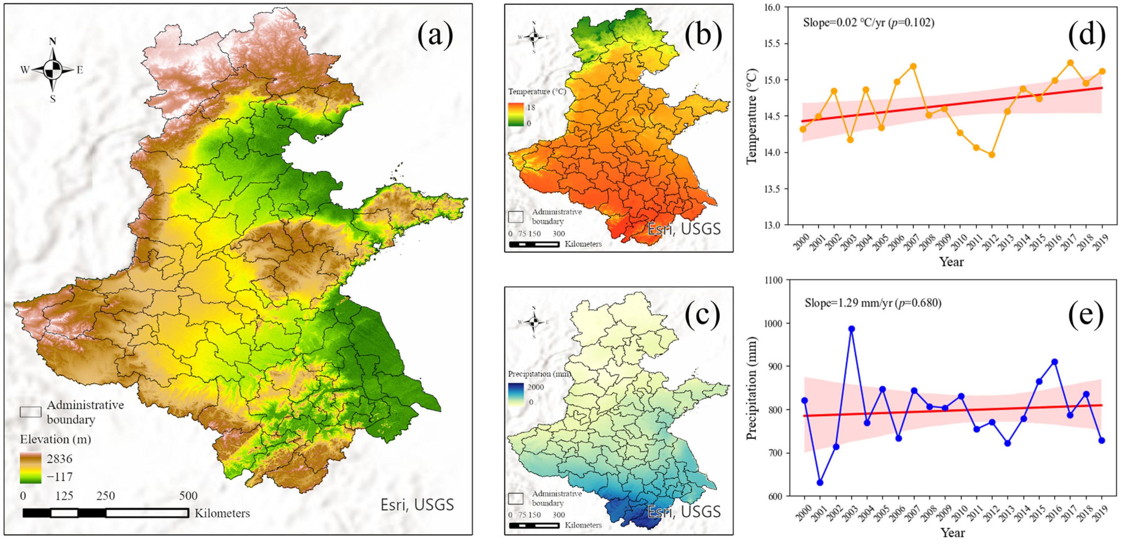
2.1. Study Area

The HHHP is a crucial grain-producing region in China, spanning across several provinces in eastern China, including Beijing, Tianjin, Hebei, Anhui, Henan, Jiangsu, and Shandong. As illustrated in Figure 1, the HHHP’s terrain is characterized by a gradual descent from high elevations in the west to lower elevations in the east, with the northern and southern areas also being higher than the central region.

The HHHP exhibits distinct north–south climatic variations. The southern region experiences warmer temperatures and higher precipitation, while the northern region is comparatively cooler and drier. Between 2000 and 2019, the average temperature across the HHHP ranged from 0 °C to 18 °C, while the annual precipitation varied between 0 mm and 2000 mm. The region experienced a warming trend during this period, while precipitation showed no clear directional change. These climatic shifts, particularly the rising temperatures, may influence crop growth and yields by affecting soil moisture, evapotranspiration, and growing season length.

2.2. Data Collection and Preprocessing

2.2.1. Wheat Phenology and Distribution Data

The winter wheat phenology and distribution data used in this study were sourced from the ChinaCropPhen1km dataset [54]. This dataset utilizes the GLASS LAI product and generates 1 km resolution phenology products for various crops, including maize, rice, and wheat, across China. The data span from 2000 to 2019 and provide detailed insights into the growth stages of winter wheat. For winter wheat, the dataset includes three critical phenological periods: GR (green-up date), HE (heading date), and MA (maturity date). The average RMSE (root-mean-square error) for these three key phenological periods is approximately 5.5 days, which is sufficient for the needs of this study. Since this research focuses solely on winter wheat, areas with a heading date (HE) greater than 180 days were excluded, as these correspond to areas where spring wheat is typically grown. This exclusion ensures that this study accurately targets winter wheat cultivation.

2.2.2. Spectral Index

The MOD09A1 and MYD09A1 datasets, derived from Terra and Aqua sensors, respectively, share consistent parameters, including a spatial resolution of 500 m and a temporal resolution of 8 days. Given that crop yield is influenced by various environmental factors throughout the growing season, the stress of these factors on crops may manifest at different stages of development. Consequently, missing values in the data can introduce uncertainty and affect the final yield estimates. To address this, this study integrated data from both Terra and Aqua sensors, covering the period from 2000 to 2019.

In this study, the “QA” band was used to remove clouds. Subsequently, we used linear interpolation to fill in missing values, ensuring a continuous time series. During the time-series smoothing stage, the Savitzky–Golay (SG) [55] filter was applied using a 40-day window and a third-order polynomial. The parameters were optimized based on previous research [56] and adjusted according to the characteristics of the study area. After these preprocessing steps, a regular, cloud-free, 8-day time-series dataset was generated. To match the resolution of the wheat phenology data, all image data were resampled to a 1000 m spatial resolution. Subsequently, various vegetation indices, including the NDVI and EVI2, and indices related to water content like the NDWI, as well as NIRv, which is closely linked to photosynthesis, were calculated. These indices have been widely used in previous studies for crop yield estimation, either individually or in combination. All of these calculations and data processing tasks were performed using Google Earth Engine (GEE). The index was calculated as shown in

Table 1. Index calculated based on MODIS.

Indices	Formulation	Reference
NDVI	$NDVI={\displaystyle \frac{NIR-RED}{NIR+RED}}$	[57]
EVI	$EVI=2.5\times {\displaystyle \frac{NIR-RED}{NIR+6\cdot RED-7.5\cdot BLUE+1}}$	[58]
EVI2	$EVI2={\displaystyle \frac{2.5\cdot (NIR-RED)}{NIR+RED\cdot 2.4+1}}$	[59]
NDWI	$NDWI={\displaystyle \frac{NIR-SWIR}{NIR+SWIR}}$	[60]
NIRv	$NIRv=NDVI\cdot NIR$	[61]

.

2.2.3. LAI and FPAR

The LAI data used in this study were derived from the Sensor-Independent LAI dataset [62], which is based on the Terra, Aqua, and VIIRS LAI datasets. This dataset enhances the quality of LAI data by filtering low-quality inversion values and using the spatial–temporal tensor (ST-Tensor) method to fill in missing values. This approach results in a sensor-independent LAI product, which has shown improved accuracy in measured data verification and enhanced time-series stability compared to MODIS and VIIRS LAI products. The dataset offers spatial resolutions of 500 m, 5 km, and 0.05°, as well as temporal resolutions of 8 days and 2 months, making it suitable for the needs of this study. The LAI dataset demonstrates good accuracy, with an RMSE of 0.84 and an R² of 0.72.

The FPAR data used in this study came from the HiQ-FPAR dataset [63]. This dataset filters out low-quality FPAR data and uses the Spatiotemporal Information Composition Algorithm (STICA) method to generate more accurate FPAR values than the Sensor-Independent FPAR (SI-FPAR) dataset. The HiQ-FPAR dataset provides data at 500 m and 5 km resolutions, with a temporal resolution of 8 days, spanning from 2000 to 2023. The FPAR dataset has an RMSE of 0.13 and an R² of 0.72.

To maintain consistency with the temporal resolution of other data in this study, the LAI and FPAR datasets were resampled to a 1 km resolution. The combined dataset from 2000 to 2019 was used to gather wheat growing season data, ensuring compatibility across the various remote sensing datasets used for yield estimation.

2.2.4. Statistical Yearbooks

The yield data for this study were obtained from the China Economic and Social Big Data Research Platform (https://data.cnki.net/, accessed on 26 December 2024). Winter wheat production data at both the municipal and county levels for the study area, from 2000 to 2019, were collected. Data from both levels were used for filtering to remove outliers. For administrative districts with unavailable yield records, yields were estimated by dividing the total production by the planted area. The dataset was then split into training and validation sets at an 8:2 ratio, with municipal data used for initial yield estimation and calibration, while county-level data served for accuracy verification.

2.2.5. Winter Wheat Yield Dataset

The ChinaWheatYield30m dataset, generated using Landsat, Sentinel-2, and ERA5 data, employs a hierarchical linear model and features a spatial resolution of 30 m, with a temporal range from 2016 to 2021 [12]. The GlobalWheatYield4km dataset has a spatial resolution of 4 km, a temporal range from 1982 to 2020, and R values ranging from 0.4 to 0.8 at the sub-national scale [13].

2.2.6. Temperature and Precipitation Data

Temperature and precipitation data [64] were obtained from the National Earth System Science Data Center (https://www.geodata.cn, accessed on 26 December 2024) at a spatial resolution of approximately 1 km. Both datasets have a monthly temporal resolution, covering the period from 1901 to 2023. Given that winter wheat growth and harvest in this region primarily occur between February and June, this study utilized data from these months for the years 2000 to 2019.

2.3. Methods

Figure 2 illustrates the technical workflow of this study. The process began by filling missing values in the MODIS data and removing outliers using interpolation and SG filtering to prevent data gaps from distorting the average values. Next, multi-temporal indicators were calculated, and the average values for two key phenological periods were determined based on phenological data. At the municipal level, statistical analyses were conducted for Random Forest modeling. The trained model was then applied to generate initial yield estimates from the remote sensing imagery. To enhance accuracy and ensure that the initial yields better reflected the actual production, the initial yields were calibrated using statistical yearbook yield data. Finally, the dataset was evaluated through comparisons with existing datasets and county-level statistical records to assess its accuracy and reliability. Additionally, the effects of temperature and precipitation on yield were analyzed to provide insights into climate–yield interactions.

2.3.1. Development and Accuracy Assessment of HHHWheatYield1km

• Random Forest Modeling

Random Forest (RF) is a widely used machine learning algorithm based on ensemble learning, particularly in remote sensing yield estimation [65,66]. This method enhances model accuracy and robustness by constructing multiple decision trees and combining their prediction results. In this study, a series of experiments were conducted, and it was found that the model accuracy plateaued when the number of trees approached 100. Therefore, the numberOfTrees parameter was set to 100 to ensure the robustness of the results, minimize the risk of overfitting, and maintain computational efficiency.

• Calibration of Yield Data

Due to potential inconsistencies arising from natural disasters, management practices, crop varieties, and other factors, directly establishing a statistical relationship between remotely sensed indicators and yields may overlook their influence on yield variability. To address this, the initial yield estimates were calibrated using statistical data, based on the assumption that statistical yearbook records represent actual yields after accounting for these various influencing factors. Additionally, this approach assumes that the relative differences in yields among individual pixels within the same administrative division remain unchanged. Inspired by previous studies [67,68], the calibration was performed using the following formula:

$$\begin{array}{c}{Y}_{i,j}^{\prime }={\displaystyle \frac{Y_{i,j}}{\frac{{\sum }_{i=1}^n{Y}_{i,j}}{n}}}\cdot Y_j\end{array}$$

(1)

where $Y_{i,j}$ represents the initial yield of the i-th winter wheat pixel in the j-th municipality, $Y_{i,j}^{\prime }$ represents the calibrated yield of the i-th winter wheat pixel in the j-th municipality, $Y_j$ represents the winter wheat yield data in the statistical yearbook of the municipality, and n represents the number of winter wheat pixels in the municipality.

• Accuracy Evaluation

Product accuracy was assessed using multiple data sources: (1) county-level statistical yearbook data, and (2) a comparative analysis with existing datasets (GlobalWheatYield4km, and HHHWheatYield1km). The HHHWheatYield1km dataset developed in this study features a 1 km spatial resolution and covers the period from 2000 to 2019. To evaluate spatial trends, the average values of all three datasets were compared for the overlapping period of 2016 to 2019. Additionally, the spatial trends of GlobalWheatYield4km and HHHWheatYield1km were analyzed over their longer common temporal coverage from 2000 to 2019.

The accuracy of the results was evaluated using key statistical metrics, including the correlation coefficient (R), root-mean-square error (RMSE), and mean relative error (MRE) [69,70,71]. A higher R value indicates a stronger linear relationship between the observed and predicted values, reflecting better model performance. Lower RMSE and MRE values suggest reduced prediction errors, indicating closer agreement between the estimated and actual yields. Together, these metrics provide a comprehensive evaluation of the dataset’s reliability and predictive accuracy.

$$\begin{array}{c}R={\displaystyle \frac{{\sum }_{i=1}^n(y_i-\overline{y})(\widehat{y_i}-\overline{\widehat{y}})}{\sqrt{{\sum }_{i=1}^n{\left(y_i-\overline{y}\right)}^2}\cdot \sqrt{{\sum }_{i=1}^n{\left(\widehat{y_i}-\overline{\widehat{y}}\right)}^2}}}\end{array}$$

(2)

$$\begin{array}{c}RMSE=\sqrt{{\displaystyle \frac{1}{n}}{\displaystyle {\sum }_{i=1}^n}{\left(y_i-\widehat{y_i}\right)}^2}\end{array}$$

(3)

$$\begin{array}{c}MRE={\displaystyle \frac{1}{n}}{\displaystyle {\sum }_{i=1}^n}\left|{\displaystyle \frac{y_i-\widehat{y_i}}{y_i}}\right|\cdot 100\%\end{array}$$

(4)

where $y_i$ represents the observed yield from statistical yearbooks, $\widehat{y_i}$ represents the predicted yield, $\overline{y}$ and $\overline{\widehat{y}}$ denote the mean observed and predicted values, respectively, and $n$ is the total number of samples.

2.3.2. Analysis of Factors Affecting Winter Wheat Yield

Geodetector is a robust, nonlinear approach for analyzing the influence of different driving factors and their interactions. It is based on the principle that if one factor significantly affects another, their spatial distributions should exhibit similarity [72]. The method involves categorizing all samples into different levels and analyzing the variance within each subsample compared to the total variance of all samples. If the sum of the subsample variances is smaller than the total variance, this indicates the presence of spatial heterogeneity. This approach has been widely applied in studies of vegetation dynamics, atmospheric pollutant distribution, and landslide susceptibility mapping [73,74,75].

To better understand the factors influencing winter wheat yield in the HHHP at a finer spatial scale, the analysis was conducted separately for different provincial administrative divisions. Specifically, Beijing, Tianjin, and Hebei were grouped as a single region—Beijing–Tianjin–Hebei (Jingjinji)—while Anhui, Henan, Shandong, and Jiangsu were analyzed independently, resulting in a total of five regional assessments. The “GD” package in R was used for the analysis. Parameter optimization [76] was conducted through the application of various classification methodologies, including “equal”, “natural”, “quantile”, “geometric”, and “sd”. These methods were utilized to categorize continuous variables into three to seven distinct classes, thereby facilitating the attainment of optimal q-values.

• Factor detector

$$\begin{array}{c}q=1-{\displaystyle \frac{{\sum }_{h=1}^L{N}_h{\sigma }_h^2}{N{\sigma }^2}}\end{array}$$

(5)

where $h$ represents the number of categorized variables, and $L$ is the maximum number of categories into which the variables are classified. $N_h$ and $N$ denote the number of cells in the $h$-th stratum and the entire study area, respectively; ${\sigma }_h^2$ and ${\sigma }^2$ represent the variance within the $h$-th category and the total variance of the entire study area, respectively. The q-value quantifies the explanatory power of a driving factor on the spatial distribution of winter wheat yields, ranging from 0 to 1. A higher $q$ value indicates a stronger explanatory power of the factor.

• Interaction detector

Interaction detectors are used to evaluate how the explanatory power of two factors changes when they act together. For example, when analyzing the effects of the variables X₁ and X₂ on Y, a superposition analysis is conducted to determine the explanatory power of (X₁∩X₂) on Y. By combining the stratification of X₁ and X₂, the joint influence of both factors on Y can be assessed. This approach enabled a more detailed analysis of the complex interactions between temperature and precipitation in influencing winter wheat yields in this study.

2.3.3. Trend Analysis

The Mann–Kendall (MK) test is a widely used nonparametric method for detecting trends in climatic and hydrological time series [77,78,79]. However, in the context of this study, the yield data exhibit autocorrelation, which can increase the likelihood of falsely detecting significant trends [80]. To address this issue, we first applied variance correction [81] to remove the effect of autocorrelation, before performing the MK test to ensure more reliable trend detection.

3. Results

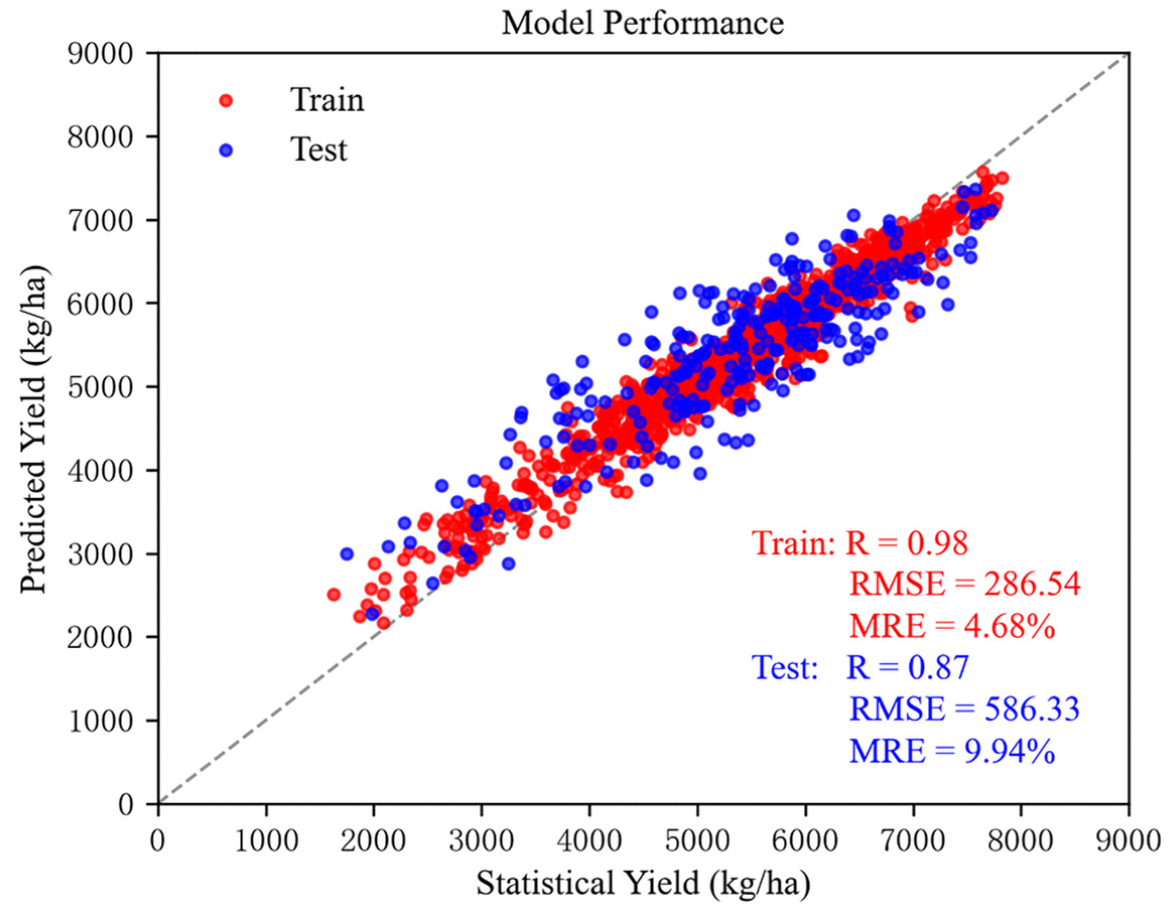
3.1. Accuracy Assessment of the Model for Initial Yield Generation

The performance of the model on both the training set and test set is presented in Figure 3. On the training set, the model exhibited high prediction accuracy, with an R value of 0.98, an RMSE of 286.54 kg/ha, and an MRE of 4.68%. These results indicate that the model effectively captures the nonlinear relationships in the training data, demonstrating strong fitting capability. On the test set, although the prediction performance decreased, the model still achieved notable accuracy, with an R value of 0.87, an RMSE of 586.33 kg/ha, and an MRE of 9.94%. This demonstrates that the model possesses reasonable generalization ability for unseen data, enabling accurate prediction of yield distributions at the municipal scale.

3.2. Accuracy Evaluation of Calibrated Yield Data

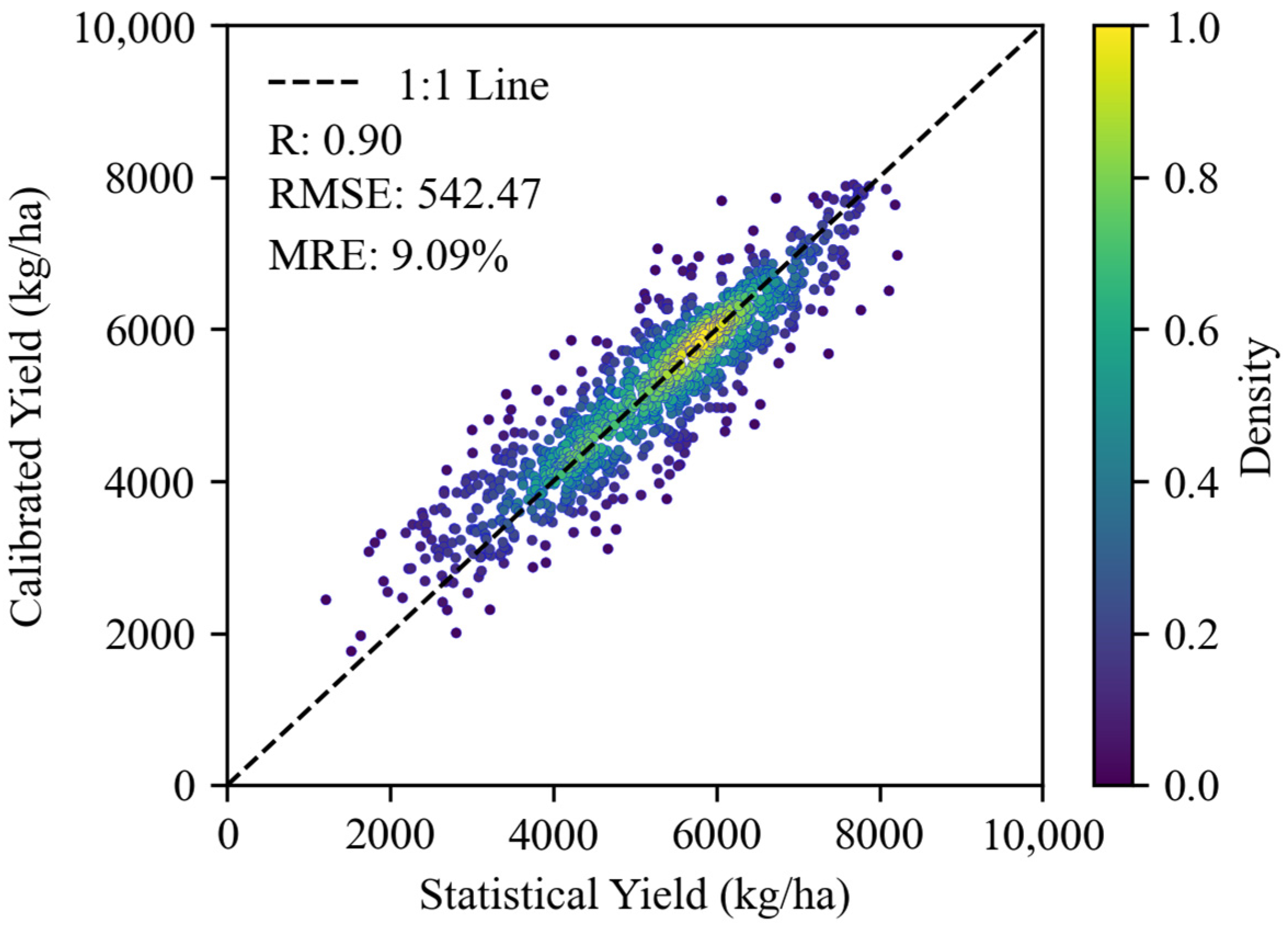
3.2.1. Accuracy Evaluation with County-Level Statistical Data

Figure 4 presents the accuracy validation results of HHHWheatYield1km at the county scale. The validation shows a strong correlation between HHHWheatYield1km and county-level statistical yearbook data, with an R value of 0.90. Error analysis reveals an RMSE of 542.47 kg/ha and an MRE of 9.09%, indicating that the dataset effectively captures spatial details at the county scale and reasonably reflects actual conditions.

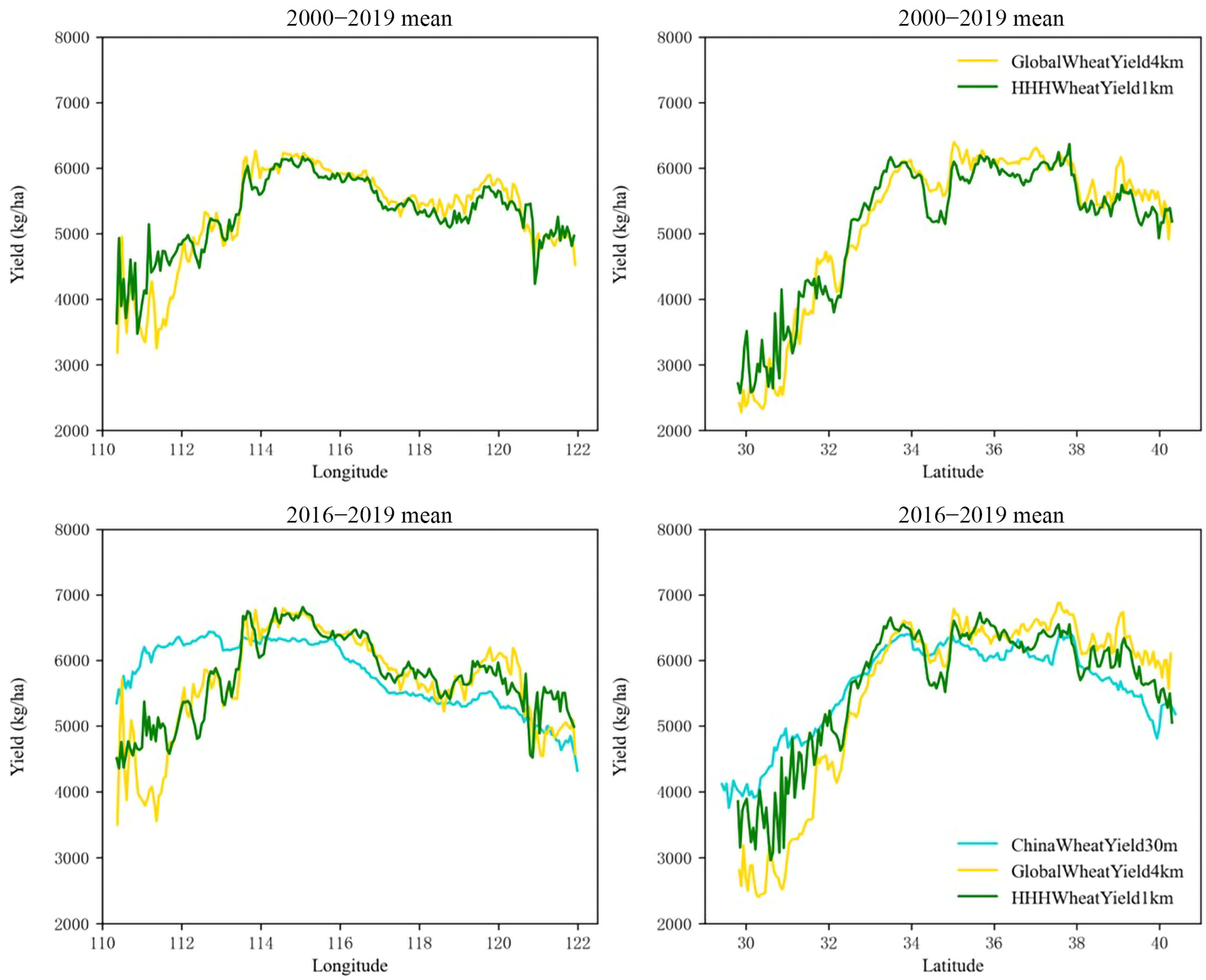
3.2.2. Accuracy Evaluation with Existing Datasets

Figure 5 illustrates the average spatial distribution characteristics of three wheat yield datasets across different time periods (2016–2019 and 2000–2019). While the spatial patterns vary among the datasets, certain trends are evident. Both the HHHWheatYield1km and GlobalWheatYield4km datasets exhibit a distribution pattern of lower yields in the north and higher yields in the south. In contrast, the ChinaWheatYield30m dataset shows an opposite trend, with higher yields in the north and lower yields in the south. According to statistical yearbook data, the average yield per unit area in northeastern regions, such as Heze, from 2016 to 2019 was approximately 6000 kg/ha, while in southern regions, such as Shangqiu and Zhoukou, the average yield exceeded 7000 kg/ha. After corrections, the HHHWheatYield1km dataset aligns more closely with the actual yield distribution, accurately reflecting regional yield variations.

Figure 6 presents the spatial trend of average wheat yield per unit area in both the longitudinal and latitudinal directions, based on three datasets—HHHWheatYield1km, GlobalWheatYield4km, and ChinaWheatYield30m—across the periods 2000–2019 and 2016–2019. The yield trends for the two time periods exhibit a high level of consistency, and the longitudinal and latitudinal yield distributions of the three datasets are largely aligned. Longitudinally, the highest yield values are concentrated around 114°E, corresponding to the central and eastern regions of Henan Province, which exhibit high productivity. In contrast, data from other provinces exhibit relatively lower yields. Latitudinally, the peak yield values are observed near 36°N and 37.8°N, respectively. Although differences exist among the datasets in finer details—due to variations in resolution, crop distribution data, and source imagery—all of the datasets display similar spatial distribution trends. This strong agreement underscores the reliability and applicability of the HHHWheatYield1km dataset, confirming its consistency with other datasets in capturing the spatial characteristics of wheat yield distribution.

Figure 7 presents the validation results of the three datasets against county-level statistical data in the HHHP. Among the datasets, HHHWheatYield1km achieves the highest accuracy in this region, with an MRE of 9.09%. In contrast, ChinaWheatYield30m shows lower accuracy, with an MRE of 29.88%. This discrepancy may be attributed to differences in spatial scale [82]. HHHWheatYield1km converts yield estimates from the administrative scale to a coarser 1 km resolution, partially preserving the aggregate characteristics of the statistical data. In contrast, ChinaWheatYield30m is developed at a finer 30 m resolution, where the scale mismatch becomes more pronounced and challenging to reconcile. Additionally, HHHWheatYield1km was specifically trained using data from the HHHP, which may explain its superior performance within this region. The performance of GlobalWheatYield4km, with accuracy falling between the other two datasets, suggests that its coarser resolution reduces the sensitivity to scale mismatches but may limit spatial detail. These findings highlight the persistent challenge of reconciling scale differences between administrative statistics and pixel-level remote sensing estimates, pointing to the need for further methodological exploration in future research.

In the comprehensive analysis, the three datasets exhibited a relatively consistent spatial distribution pattern (Figure 8). This uniformity was evident across all datasets; however, the lower-resolution products (1 km and 4 km) showed noticeable amalgamation of land-cover types within individual pixels. Such aggregation allows multiple surface features—such as woodland, grassland, and impervious areas—to coexist within a single pixel, potentially leading to inaccuracies in yield estimation. Nevertheless, at the administrative scale, this heterogeneity is somewhat mitigated, making the low-resolution datasets more representative of regional averages. In contrast, higher-resolution datasets are more prone to errors introduced during the transition between pixel-level and administrative-unit scales. This issue is especially pronounced in the finest-resolution dataset, which shows larger deviations when validated against county-level statistics. While the ChinaWheatYield30m dataset offers higher spatial resolution, the HHHWheatYield1km dataset compensates for this limitation by providing a longer temporal coverage, making it more suitable for long-term trend analysis.

In summary, the comparative analysis revealed that the HHHWheatYield1km dataset demonstrates a notable consistency with existing datasets, such as GlobalWheatYield4km and ChinaWheatYield30m, regarding overall spatial distribution trends. However, due to its more advanced correction processes, HHHWheatYield1km achieves higher accuracy in capturing localized yield variations, aligning more closely with the observed data. This indicates that, while maintaining broader spatial distribution trends, HHHWheatYield1km improves the precision of yield estimation at the local scale. As a result, this dataset provides more reliable support for regional yield analysis and informed agricultural decision-making.

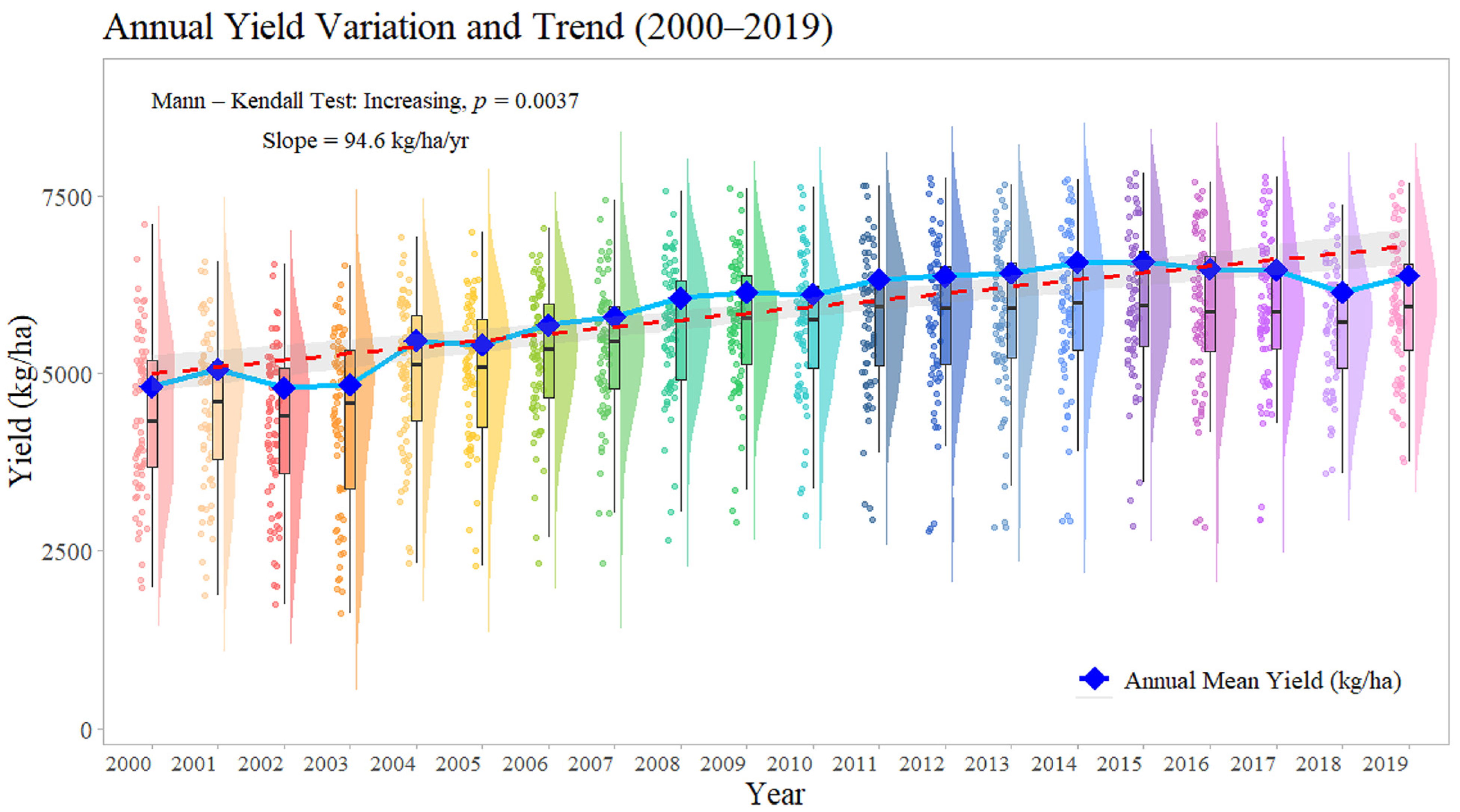
3.3. Temporal Trends of Winter Wheat Yields

Figure 9 presents the temporal trend of wheat yields in the study area from 2000 to 2019. The results show a gradual upward trend in winter wheat yields prior to 2010. After 2010, the yields stabilized, and regional yield disparities gradually diminished. This reduction in regional yield differences can likely be attributed to improvements in agricultural management and technological advancements, such as the development of high-standard farmland and advancements in fertilization techniques. These measures have likely mitigated yield gaps caused by regional environmental suitability, contributing to more uniform wheat production across different areas. Additionally, we calculated the annual average of HHHWheatYield1km at the pixel scale. The results revealed a significant upward trend in the average winter wheat yield across the region from 2000 to 2019. Linear regression analysis indicated that the average yield increased at a rate of 94.6 kg/ha per year.

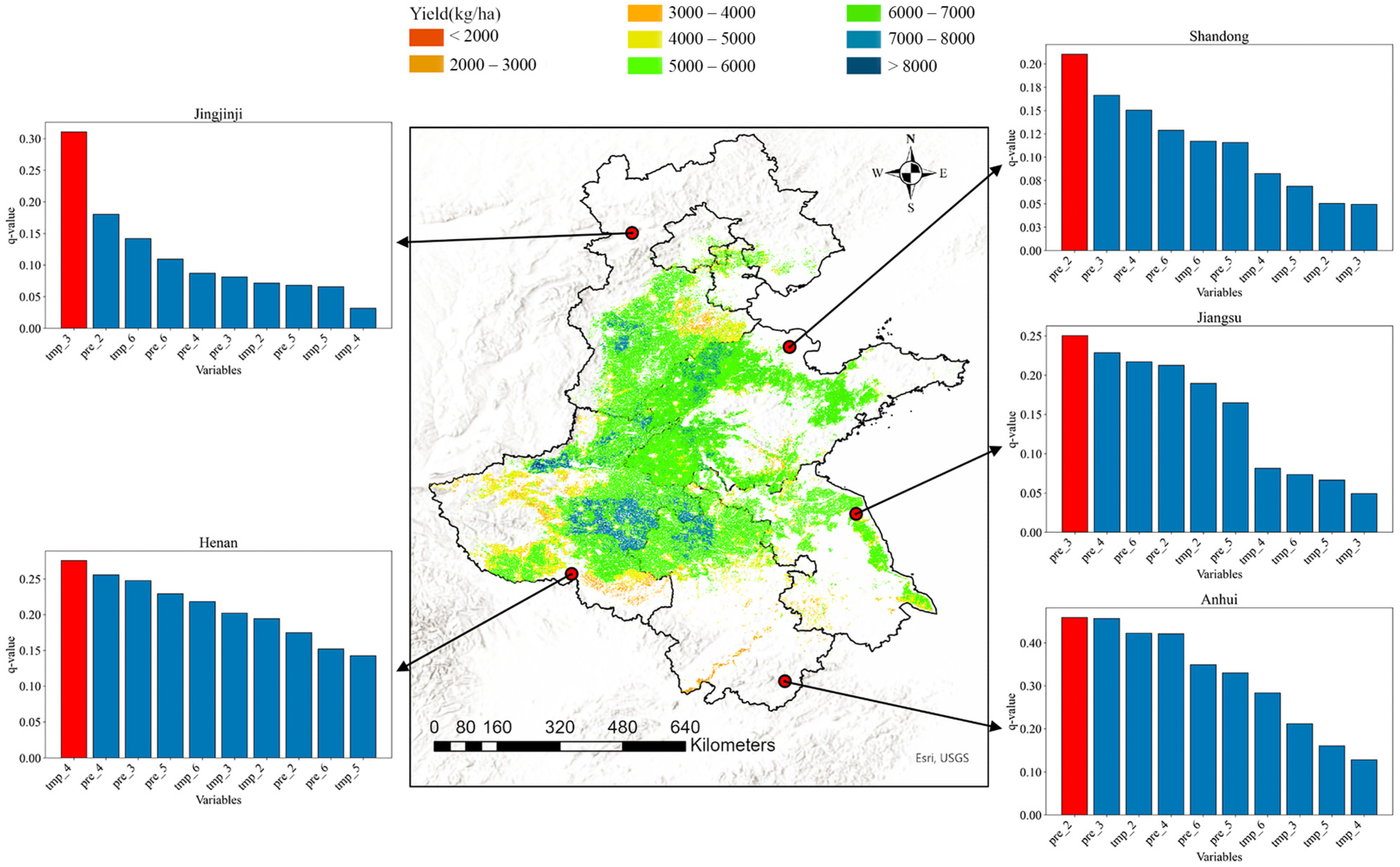
3.4. Spatial Pattern and Influencing Factors of Winter Wheat Yield

Figure 10 illustrates the spatial distribution of average winter wheat yields from 2000 to 2019 and the influence of temperature and precipitation on yields across different regions. High-yield regions are primarily concentrated in the eastern part of Henan Province, which demonstrates superior agricultural conditions and advanced management practices. This region stands out for its favorable environment, including fertile soils and adequate water availability, which contribute to its high yield per unit area. Conversely, the western mountainous areas exhibit relatively low yields, constrained by challenging terrain and less favorable climatic conditions. The rest of the region shows medium-to-high wheat yields, with a relatively uniform distribution.

The factor detector results indicate that inland provinces, such as Henan and Anhui, are significantly constrained by natural factors. Anhui exhibits the highest sensitivity of winter wheat yield to precipitation (pre_2, q = 0.459), while Henan shows a more balanced influence of both temperature and precipitation. In contrast, the eastern coastal provinces, Shandong and Jiangsu, experience weaker climatic constraints, with a lower explanatory power of dominant factors (Shandong: pre_2, q = 0.210; Jiangsu: pre_3, q = 0.250). The Jingjinji area follows a temperature-dominant pattern (tmp_3, q = 0.310).

The interaction detector results (Figure 11) further highlight that factor interactions enhance the explanatory power of yield variations, although the overall trend mirrors the factor detector findings. The strongest explanatory power is observed for the interaction of tmp_02 and tmp_06 in Anhui (q = 0.583) and pre_2 and pre_5 in Henan (q = 0.545). In contrast, the explanatory power of dominant interactions in coastal regions generally remains lower than 0.35 (e.g., the strongest interaction in Shandong is tmp_06 and pre_2, q = 0.277; in Jiangsu, tmp_4 and pre_3, q = 0.328). These results emphasize the importance of developing heat-resistant crop varieties and enhancing the irrigation infrastructure in Anhui. In Henan, it is equally critical to investigate the influence of precipitation and improve irrigation practices. In coastal regions, where non-climatic factors play a more prominent role, promoting precision agriculture is essential. Farmers in these areas often enhance their productivity through adjustments in cropping calendars and the adoption of advanced water management strategies. Moreover, it is important to recognize that precipitation and temperature have varying impacts on crops at different phenological stages. This highlights the need for stage-specific management approaches tailored to the distinct requirements of each growth phase.

4. Discussion

4.1. Importance of Predictor Variables

Figure 12 shows the distribution of different characteristic indicators during the modeling of two phenological stages (stage 1 and stage 2) of winter wheat growth. The results highlight that FPAR is the most important indicator in the second stage, surpassing the other indicators in importance. FPAR is closely related to photosynthesis and significantly influences yield prediction due to its role in evaluating photosynthetic rates [83,84].

Indicators from the second stage contribute significantly more (69.5%) to the total importance compared to the first stage (30.5%). This indicates that the indicators from the second stage play a more crucial role in determining the final yield. MODIS’s low resolution and sensitivity to background elements like soil and moisture reduce the significance of early-stage indicators [85].

Interestingly, despite the overall lower importance of early-stage indicators, NDWI_1 ranks second in importance among all characteristics. The NDWI’s sensitivity to water reflects its critical role in influencing crop development during the early growth stages, highlighting the significant impact of water availability on winter wheat growth [27]. The first stage primarily corresponds to the nutritional growth phase, while the second stage is focused on the reproductive phase. The reproductive stage, being closer to the final yield, is critical for dry matter accumulation [86], making remote sensing features during this period more directly reflective of yield formation. In contrast, the nutritional growth stage has a more indirect impact, as it lays the foundation for subsequent reproductive growth.

The current approach characterizes yield purely from the perspective of crop growth, based on two key assumptions: (1) municipal statistical yield data can effectively reflect spatial patterns in agricultural production, and (2) the environmental homogeneity within administrative units provides a reasonable basis for yield inversion at the pixel scale. However, agricultural systems exhibit spatial heterogeneity even within municipal boundaries. Local variations in meteorological conditions (e.g., temperature gradients), crop variety diversity, topographic complexity, and soil property differences can all affect the accuracy of yield estimates [87]. Zhou et al. [88] argued that climatic variables often have greater explanatory power than remote sensing data in yield prediction models, and that combining both can improve model performance. In this study, climate variables were intentionally excluded to isolate the independent contribution of remotely sensed signals, although this may have introduced systematic bias at the pixel level.

These uncertainties are further compounded by the nonlinear response of crop growth to climatic factors. Studies have shown that increased temperatures can shorten critical growth stages of winter wheat—such as the grain-filling period—thereby reducing the accumulation of photosynthates [89,90]. Additionally, temperature effects on crops are often delayed [91], limiting remote sensing data’s ability to capture the real-time impacts of temperature stress. Consequently, pixel-level yield estimates within administrative boundaries may be over- or underestimated. For example, in high-temperature areas, yields may be overestimated due to the accelerated wheat development, which is not fully captured by vegetation indices. Similarly, in regions with lower management levels, the model may slightly overestimate yields due to its representation of regional averages [92]. Despite these limitations, calibration at the municipal level helps mitigate large-scale heterogeneity. However, intra-municipal heterogeneity remains a significant challenge. Future research will aim to address this issue by acquiring more representative ground samples and refining the calibration process within municipal boundaries.

4.2. Advantages of HHHWheatYield1km

The HHHWheatYield1km dataset offers a valuable resource for studying food production under global challenges like climate change, increasing climate risks, and population growth. By providing accurate winter wheat yield estimates, the dataset improves assessment reliability and reduces uncertainties compared to traditional datasets that rely heavily on meteorological variables. Unlike interpolated meteorological data, which often suffer from coarse spatial resolution and pixel-level errors, HHHWheatYield1km employs independent variables to estimate yield, thereby minimizing potential biases in the modeling process [93,94].

This dataset was developed based on specific remote sensing and phenological variables and was calibrated using statistical yield data to ensure close alignment with the observed outcomes. The calibration process resembles spatial disaggregation, whereby yield statistics at the administrative level are refined to match the spatial resolution of remote sensing imagery. For instance, Chen et al. [67] applied RF to create weight coefficients for the spatial downscaling of solar-induced chlorophyll fluorescence (SIF). However, a key difference in this research is the spatial distribution of crops, which can lead to errors when directly downscaling yield data, due to variations in crop classification accuracy and other factors. Therefore, this study employed yield per unit area for calibration, considering the error in crop classification accuracy to improve the accuracy of the estimates. This method helps address the challenges associated with directly downscaling yield data and ensures more reliable results in the estimation process.

The HHHWheatYield1km exhibits several significant attributes in comparison to existing datasets (

Table 2. Summary of information on different wheat yield datasets.

Dataset	Region	Spatial Resolution	Temporal Coverage
GlobalWheatYield4km	Global	4 km	1982–2020
ChinaWheatYield30m	China	30 m	2016–2021
HHHWheatYield1km	Huang-Huai-Hai Plain	1 km	2000–2019

). Temporally, it spans a longer period (2000–2019) compared to ChinaWheatYield30m, which is limited to 2016–2021. In terms of spatial resolution, it achieves a finer resolution (1 km) than the global GlobalWheatYield4km dataset (4 km). A critical distinguishing characteristic of this dataset is its independence from climate variables in its modeling, rendering it particularly advantageous for investigations focused on evaluating the effects of climate change on crop yields without introducing circular reasoning. Nonetheless, it is important to acknowledge that the current dataset is restricted in spatial coverage, being limited to the HHHP, which is narrower than the national scope of ChinaWheatYield30m and the global extent of GlobalWheatYield4km. Given that this study primarily assesses the feasibility of the program, future endeavors will aim to produce a dataset with broader coverage and enhanced resolution.

HHHWheatYield1km focuses on accurately predicting crop yields without considering climate variables. This modeling approach allows for the independent assessment of environmental influences on yield variability and provides a robust framework for analyzing spatial and temporal fluctuations. This method also facilitates the integration of data across the administrative and pixel-level scales, producing outputs that more closely reflect on-the-ground conditions. Due to scale effects [95], predictions at the administrative level often achieve higher accuracy than those at the image level. For example, Cao et al. [42] reported that the average R² for predicting winter wheat yields at the county scale was ≥ 0.85, but this value dropped to 0.66 when applied at the field scale.

Therefore, a feasible future direction is to first perform yield prediction at the administrative scale and then incorporate remote sensing imagery to downscale the results. This would allow both regional-scale trends and pixel-level spatial heterogeneity to be captured. Yield values at the pixel scale could then support targeted food security early warning systems and offer practical guidance to farmers for implementing site-specific yield improvement measures.

4.3. Heterogeneity Analysis of the Effect of Climatic Factors on Winter Wheat Yields

The effects of temperature and precipitation on winter wheat yields are complex and spatially heterogeneous across the HHHP. Increased temperatures can shorten the phenological period of winter wheat, reducing the time available for nutrient accumulation, and ultimately leading to lower yields [96]. Meanwhile, the demand for water rises sharply in the late reproductive stage, making winter wheat highly susceptible to drought stress [97], which can further exacerbate yield losses [98]. These climatic factors interact with regional environmental conditions and agricultural practices, creating distinct spatial patterns in their influence on winter wheat yields. The inland provinces, such as Anhui and Henan, are characterized by a continental climate with significant temporal and spatial variability in precipitation. These regions experience frequent water shortages, increasing their dependence on precipitation for stable wheat production [99,100]. The high variability in rainfall, coupled with the limited availability of irrigation resources, results in stronger climatic constraints on yield, as reflected by higher q-values in the factor detector analysis. In contrast, the coastal provinces of Shandong and Jiangsu are influenced by the East Asian monsoon, which brings hot, humid summers and cold, dry winters [101,102]. These climatic conditions provide relatively stable thermal and hydrological conditions, reducing the dependence of wheat production on specific climatic factors [103]. The weaker climatic constraints in coastal regions are reflected in the lower q-values of temperature and precipitation, indicating that other factors, such as agricultural management and technological advancements, play a more dominant role in determining yield outcomes.

In addition to climate, agricultural adaptation measures have played a crucial role in shaping winter wheat yields in the region. Previous studies have demonstrated that changes in agronomic practices, such as the adoption of improved wheat varieties and adjustments in sowing periods, have significantly influenced yield trends. Xiao and Tao [104], using field trial data from multiple sites in the North China Plain, combined with crop modeling, found that varietal renewal contributed to yield increases of 12.2–22.6%, whereas the overall contribution of climate change to yield was -3.0% to 3.0%. This suggests that, while climate change poses challenges to winter wheat production, improvements in agricultural management have mitigated its negative impacts and even led to yield increases in many regions.

The HHHP is dependent on irrigation for agricultural production [105]; however, the region faces persistent challenges related to water availability [106]. The heterogeneity in the influence of temperature and precipitation on winter wheat yields underscores the need for region-specific agricultural strategies to enhance resilience and sustainability. In inland provinces, where climate variability is higher and water scarcity is a major challenge, efforts should focus on improving water-use efficiency through the adoption of drought-resistant wheat varieties and advanced irrigation techniques. Precision agriculture and soil moisture conservation practices can further enhance yield stability in these regions. Conversely, in coastal areas, where climatic conditions are more stable and natural constraints are weaker, the focus should be on optimizing resource utilization and enhancing wheat productivity through genetic improvements and agronomic innovations. By balancing climate adaptation strategies with resource optimization, winter wheat production in the HHHP can be made more resilient to future environmental changes while sustaining high yields.

4.4. Limitations and Future Outlook

Despite the high accuracy of the HHHWheatYield1km dataset, certain uncertainties remain, primarily arising from the following factors:

(a)

MODIS Limitations: This study used MODIS data, which have lower resolution compared to Landsat and Sentinel and are more prone to mixed pixel issues. However, to maintain scale consistency with key input data (LAI, FPAR, ChinaCropPhen1km), the use of MODIS was necessary. Future research will prioritize the integration of higher-resolution and multi-source remote sensing data. This will include exploring the utility of SAR data for yield estimation [107,108], applying spatiotemporal fusion algorithms to overcome current resolution constraints, thereby enabling more precise yield mapping.

(b)

Scale Differences: The training data employed in this study were based on municipal-level agricultural statistics aggregated by administrative boundaries, whereas yield estimates were produced at the pixel level. This spatial scale mismatch introduces inherent uncertainty. Although the machine-learning-based spatial disaggregation and statistical calibration approaches adopted here help to reduce this issue, they do not fully eliminate it. Future work should address this limitation by incorporating fine-scale data from crop growth models or field surveys at the plot or point level. These data, when integrated with machine learning techniques, can enhance pixel-level yield estimation and improve the interpretability and robustness of results across different spatial scales.

(c)

Lack of Field Validation: While the yield estimates have been validated using county-level statistics and existing yield datasets, the lack of field-level sample data restricts the ability to evaluate estimation accuracy at the pixel scale. This limitation hinders the detection and analysis of spatially localized errors. To improve the reliability and credibility of the results, future studies will involve the collection of field survey data to facilitate rigorous point-level validation.

(d)

Product Limitations: The ChinaCropPhen1km dataset used in this study is constrained by its coarse resolution, which leads to the mixing of image elements—such as agricultural with non-agricultural areas, or winter wheat with phenologically similar crops. To address this issue, future efforts should utilize higher-resolution and more precise phenological products, which will improve the accuracy of crop distribution and phenology identification.

In conclusion, spatial resolution remains a major constraint of this study, encompassing both the resolution of remote sensing imagery and the critical input datasets. Moreover, further research will be required to address the mismatch between administrative boundaries and pixel-level data, particularly in the context of scale conversion during yield estimation.

Regarding the modeling approach, the selection of the Random Forest algorithm reflects a balance between computational efficiency and predictive accuracy. Additional evaluations, as presented in the Supplementary Materials (Figure S1), demonstrate that Random Forest achieves the best overall performance among traditional machine learning methods. While deep learning models such as LSTM and CNNs exhibit marginally higher accuracy, Random Forest was preferred due to its integration compatibility with GEE, thereby enabling easier application across different regions and temporal scales. Nonetheless, as larger datasets become available and computational resources improve, deep learning approaches are expected to offer enhanced capabilities. Thus, incorporating advanced deep learning techniques constitutes an important direction for future research.

5. Conclusions

This study developed HHHWheatYield1km, a high-resolution (2000–2019) winter wheat yield dataset for China’s Huang-Huai-Hai Plain, using MODIS data and a Random Forest model. Calibrated with statistical records, this dataset demonstrated high local-scale accuracy and reliability for yield analysis, policymaking, and food security assessments, due to its independence from meteorological inputs.

Climate impacts on yields show spatial variability: Henan and Anhui are constrained by precipitation, while Shandong and Jiangsu face milder climatic limits. Yields in the Jingjinji region are sensitive to March temperature fluctuations. Region-specific strategies to enhance water-use efficiency inland and optimize agronomic practices in coastal areas are critical for sustainable production. Future efforts will focus on integrating higher-resolution remote sensing data and advanced modeling to improve dataset precision and utility.

References

- Farooq, M.S.; Uzair, M.; Raza, A.; Habib, M.; Xu, Y.; Yousuf, M.; Yang, S.H.; Ramzan Khan, M. Uncovering the Research Gaps to Alleviate the Negative Impacts of Climate Change on Food Security: A Review. Front. Plant Sci. 2022, 13, 927535. [Google Scholar] [CrossRef] [PubMed]
- King, T.; Cole, M.; Farber, J.M.; Eisenbrand, G.; Zabaras, D.; Fox, E.M.; Hill, J.P. Food Safety for Food Security: Relationship between Global Megatrends and Developments in Food Safety. Trends Food Sci. Technol. 2017, 68, 160–175. [Google Scholar] [CrossRef]
- United-Nations World Population Prospects: The 2015 Revision; Population Division of the Department of Economic and Social Affairs of the United Nations Secretariat, Department of Economic and Social Affairs: New York, NY, USA, 2015.
- Fischer, R.A.; Connor, D.J. Issues for Cropping and Agricultural Science in the next 20 Years. Field Crops Res. 2018, 222, 121–142. [Google Scholar] [CrossRef]
- Shiferaw, B.; Smale, M.; Braun, H.-J.; Duveiller, E.; Reynolds, M.; Muricho, G. Crops That Feed the World 10. Past Successes and Future Challenges to the Role Played by Wheat in Global Food Security. Food Sec. 2013, 5, 291–317. [Google Scholar] [CrossRef]
- Lu, C.; Fan, L. Winter Wheat Yield Potentials and Yield Gaps in the North China Plain. Field Crops Res. 2013, 143, 98–105. [Google Scholar] [CrossRef]
- Deryng, D.; Sacks, W.J.; Barford, C.C.; Ramankutty, N. Simulating the Effects of Climate and Agricultural Management Practices on Global Crop Yield. Glob. Biogeochem. Cycles 2011, 25, GB2006. [Google Scholar] [CrossRef]
- Jalota, S.K.; Singh, S.; Chahal, G.B.S.; Ray, S.S.; Panigraghy, S.; Bhupinder-Singh; Singh, K.B. Soil Texture, Climate and Management Effects on Plant Growth, Grain Yield and Water Use by Rainfed Maize–Wheat Cropping System: Field and Simulation Study. Agric. Water Manag. 2010, 97, 83–90. [Google Scholar] [CrossRef]
- Lobell, D.B.; Gourdji, S.M. The Influence of Climate Change on Global Crop Productivity. Plant Physiol. 2012, 160, 1686–1697. [Google Scholar] [CrossRef]
- Lesk, C.; Rowhani, P.; Ramankutty, N. Influence of Extreme Weather Disasters on Global Crop Production. Nature 2016, 529, 84–87. [Google Scholar] [CrossRef]
- Shi, W.; Wang, M.; Liu, Y. Crop Yield and Production Responses to Climate Disasters in China. Sci. Total Environ. 2021, 750, 141147. [Google Scholar] [CrossRef]
- Zhao, Y.; Han, S.; Zheng, J.; Xue, H.; Li, Z.; Meng, Y.; Li, X.; Yang, X.; Li, Z.; Cai, S.; et al. ChinaWheatYield30m: A 30m Annual Winter Wheat Yield Dataset from 2016 to 2021 in China. Earth Syst. Sci. Data 2023, 15, 4047–4063. [Google Scholar] [CrossRef]
- Zhang, Z.; Luo, Y.; Han, J.; Xu, J.; Tao, F. Estimating Global Wheat Yields at 4 Km Resolution during 1982–2020 by a Spatiotemporal Transferable Method. Remote Sens. 2024, 16, 2342. [Google Scholar] [CrossRef]
- Cheng, M.; Jiao, X.; Shi, L.; Penuelas, J.; Kumar, L.; Nie, C.; Wu, T.; Liu, K.; Wu, W.; Jin, X. High-Resolution Crop Yield and Water Productivity Dataset Generated Using Random Forest and Remote Sensing. Sci. Data 2022, 9, 641. [Google Scholar] [CrossRef]
- Peña-Gallardo, M.; Vicente-Serrano, S.M.; Quiring, S.; Svoboda, M.; Hannaford, J.; Tomas-Burguera, M.; Martín-Hernández, N.; Domínguez-Castro, F.; El Kenawy, A. Response of Crop Yield to Different Time-Scales of Drought in the United States: Spatio-Temporal Patterns and Climatic and Environmental Drivers. Agric. For. Meteorol. 2019, 264, 40–55. [Google Scholar] [CrossRef]
- Dhillon, R.; Takoo, G.; Sharma, V.; Nagle, M. Utilizing Machine Learning Framework to Evaluate the Effect of Climate Change on Maize and Soybean Yield. Comput. Electron. Agric. 2024, 221, 108982. [Google Scholar] [CrossRef]
- Butler, E.E.; Huybers, P. Adaptation of US Maize to Temperature Variations. Nat. Clim. Change 2013, 3, 68–72. [Google Scholar] [CrossRef]
- Ray, D.K.; Gerber, J.S.; MacDonald, G.K.; West, P.C. Climate Variation Explains a Third of Global Crop Yield Variability. Nat. Commun. 2015, 6, 5989. [Google Scholar] [CrossRef]
- Rowhani, P.; Lobell, D.B.; Linderman, M.; Ramankutty, N. Climate Variability and Crop Production in Tanzania. Agric. For. Meteorol. 2011, 151, 449–460. [Google Scholar] [CrossRef]
- Kira, O.; Wen, J.; Han, J.; McDonald, A.J.; Barrett, C.B.; Ortiz-Bobea, A.; Liu, Y.; You, L.; Mueller, N.D.; Sun, Y. A Scalable Crop Yield Estimation Framework Based on Remote Sensing of Solar-Induced Chlorophyll Fluorescence (SIF). Environ. Res. Lett. 2024, 19, 044071. [Google Scholar] [CrossRef]
- Qin, X.; Wu, B.; Zeng, H.; Zhang, M.; Tian, F. Global Gridded Crop Production Dataset at 10 Km Resolution from 2010 to 2020. Sci. Data 2024, 11, 1377. [Google Scholar] [CrossRef]
- Zhou, Z.; Ding, Y.; Liu, S.; Wang, Y.; Fu, Q.; Shi, H. Estimating the Applicability of NDVI and SIF to Gross Primary Productivity and Grain-Yield Monitoring in China. Remote Sens. 2022, 14, 3237. [Google Scholar] [CrossRef]
- Azzari, G.; Jain, M.; Lobell, D.B. Towards Fine Resolution Global Maps of Crop Yields: Testing Multiple Methods and Satellites in Three Countries. Remote Sens. Environ. 2017, 202, 129–141. [Google Scholar] [CrossRef]
- Becker-Reshef, I.; Vermote, E.; Lindeman, M.; Justice, C. A Generalized Regression-Based Model for Forecasting Winter Wheat Yields in Kansas and Ukraine Using MODIS Data. Remote Sens. Environ. 2010, 114, 1312–1323. [Google Scholar] [CrossRef]
- Shammi, S.A.; Meng, Q. Use Time Series NDVI and EVI to Develop Dynamic Crop Growth Metrics for Yield Modeling. Ecol. Indic. 2021, 121, 107124. [Google Scholar] [CrossRef]
- Zhang, X.; Zhang, Q. Monitoring Interannual Variation in Global Crop Yield Using Long-Term AVHRR and MODIS Observations. ISPRS J. Photogramm. Remote Sens. 2016, 114, 191–205. [Google Scholar] [CrossRef] [PubMed]
- Bolton, D.K.; Friedl, M.A. Forecasting Crop Yield Using Remotely Sensed Vegetation Indices and Crop Phenology Metrics. Agric. For. Meteorol. 2013, 173, 74–84. [Google Scholar] [CrossRef]
- Basso, B.; Liu, L. Chapter Four—Seasonal Crop Yield Forecast: Methods, Applications, and Accuracies. In Advances in Agronomy; Sparks, D.L., Ed.; Academic Press: Cambridge, MA, USA, 2019; Volume 154, pp. 201–255. [Google Scholar]
- van Diepen, C.A.; Wolf, J.; van Keulen, H.; Rappoldt, C. WOFOST: A Simulation Model of Crop Production. Soil Use Manag. 1989, 5, 16–24. [Google Scholar] [CrossRef]
- Jones, J.W.; Hoogenboom, G.; Porter, C.H.; Boote, K.J.; Batchelor, W.D.; Hunt, L.A.; Wilkens, P.W.; Singh, U.; Gijsman, A.J.; Ritchie, J.T. The DSSAT Cropping System Model. Eur. J. Agron. 2003, 18, 235–265. [Google Scholar] [CrossRef]
- Huang, J.; Ma, H.; Sedano, F.; Lewis, P.; Liang, S.; Wu, Q.; Su, W.; Zhang, X.; Zhu, D. Evaluation of Regional Estimates of Winter Wheat Yield by Assimilating Three Remotely Sensed Reflectance Datasets into the Coupled WOFOST–PROSAIL Model. Eur. J. Agron. 2019, 102, 1–13. [Google Scholar] [CrossRef]
- Mokhtari, A.; Noory, H.; Vazifedoust, M. Improving Crop Yield Estimation by Assimilating LAI and Inputting Satellite-Based Surface Incoming Solar Radiation into SWAP Model. Agric. For. Meteorol. 2018, 250–251, 159–170. [Google Scholar] [CrossRef]
- Shafiee, S.; Lied, L.M.; Burud, I.; Dieseth, J.A.; Alsheikh, M.; Lillemo, M. Sequential Forward Selection and Support Vector Regression in Comparison to LASSO Regression for Spring Wheat Yield Prediction Based on UAV Imagery. Comput. Electron. Agric. 2021, 183, 106036. [Google Scholar] [CrossRef]
- Everingham, Y.; Sexton, J.; Skocaj, D.; Inman-Bamber, G. Accurate Prediction of Sugarcane Yield Using a Random Forest Algorithm. Agron. Sustain. Dev. 2016, 36, 27. [Google Scholar] [CrossRef]
- Rischbeck, P.; Elsayed, S.; Mistele, B.; Barmeier, G.; Heil, K.; Schmidhalter, U. Data Fusion of Spectral, Thermal and Canopy Height Parameters for Improved Yield Prediction of Drought Stressed Spring Barley. Eur. J. Agron. 2016, 78, 44–59. [Google Scholar] [CrossRef]
- Cai, Y.; Guan, K.; Lobell, D.; Potgieter, A.B.; Wang, S.; Peng, J.; Xu, T.; Asseng, S.; Zhang, Y.; You, L.; et al. Integrating Satellite and Climate Data to Predict Wheat Yield in Australia Using Machine Learning Approaches. Agric. For. Meteorol. 2019, 274, 144–159. [Google Scholar] [CrossRef]
- Hou, X.; Zhang, J.; Luo, X.; Zeng, S.; Lu, Y.; Wei, Q.; Liu, J.; Feng, W.; Li, Q. Peanut Yield Prediction Using Remote Sensing and Machine Learning Approaches Based on Phenological Characteristics. Comput. Electron. Agric. 2025, 232, 110084. [Google Scholar] [CrossRef]
- Li, L.; He, Q.; Harrison, M.T.; Shi, Y.; Feng, P.; Wang, B.; Zhang, Y.; Li, Y.; Liu, D.L.; Yang, G.; et al. Knowledge-Guided Machine Learning for Improving Crop Yield Projections of Waterlogging Effects under Climate Change. Resour. Environ. Sustain. 2025, 19, 100185. [Google Scholar] [CrossRef]
- McCown, R.L.; Hammer, G.L.; Hargreaves, J.N.G.; Holzworth, D.P.; Freebairn, D.M. APSIM: A Novel Software System for Model Development, Model Testing and Simulation in Agricultural Systems Research. Agric. Syst. 1996, 50, 255–271. [Google Scholar] [CrossRef]
- Keating, B.A.; Carberry, P.S.; Hammer, G.L.; Probert, M.E.; Robertson, M.J.; Holzworth, D.; Huth, N.I.; Hargreaves, J.N.G.; Meinke, H.; Hochman, Z.; et al. An Overview of APSIM, a Model Designed for Farming Systems Simulation. Eur. J. Agron. 2003, 18, 267–288. [Google Scholar] [CrossRef]
- Cao, J.; Zhang, Z.; Tao, F.; Zhang, L.; Luo, Y.; Zhang, J.; Han, J.; Xie, J. Integrating Multi-Source Data for Rice Yield Prediction across China Using Machine Learning and Deep Learning Approaches. Agric. For. Meteorol. 2021, 297, 108275. [Google Scholar] [CrossRef]
- Cao, J.; Zhang, Z.; Luo, Y.; Zhang, L.; Zhang, J.; Li, Z.; Tao, F. Wheat Yield Predictions at a County and Field Scale with Deep Learning, Machine Learning, and Google Earth Engine. Eur. J. Agron. 2021, 123, 126204. [Google Scholar] [CrossRef]
- Koirala, A.; Walsh, K.B.; Wang, Z.; McCarthy, C. Deep Learning—Method Overview and Review of Use for Fruit Detection and Yield Estimation. Comput. Electron. Agric. 2019, 162, 219–234. [Google Scholar] [CrossRef]
- Maimaitijiang, M.; Sagan, V.; Sidike, P.; Hartling, S.; Esposito, F.; Fritschi, F.B. Soybean Yield Prediction from UAV Using Multimodal Data Fusion and Deep Learning. Remote Sens. Environ. 2020, 237, 111599. [Google Scholar] [CrossRef]
- Fan, H.; Liu, S.; Li, J.; Li, L.; Dang, L.; Ren, T.; Lu, J. Early Prediction of the Seed Yield in Winter Oilseed Rape Based on the Near-Infrared Reflectance of Vegetation (NIRv). Comput. Electron. Agric. 2021, 186, 106166. [Google Scholar] [CrossRef]
- Moriondo, M.; Maselli, F.; Bindi, M. A Simple Model of Regional Wheat Yield Based on NDVI Data. Eur. J. Agron. 2007, 26, 266–274. [Google Scholar] [CrossRef]
- Soriano-González, J.; Angelats, E.; Martínez-Eixarch, M.; Alcaraz, C. Monitoring Rice Crop and Yield Estimation with Sentinel-2 Data. Field Crops Res. 2022, 281, 108507. [Google Scholar] [CrossRef]
- Zhang, Q.; Cheng, Y.-B.; Lyapustin, A.I.; Wang, Y.; Gao, F.; Suyker, A.; Verma, S.; Middleton, E.M. Estimation of Crop Gross Primary Production (GPP): fAPARchl versus MOD15A2 FPAR. Remote Sens. Environ. 2014, 153, 1–6. [Google Scholar] [CrossRef]
- Yu, Y.; Yang, X.; Guan, Z.; Zhang, Q.; Li, X.; Gul, C.; Xia, X. The Impacts of Temperature Averages, Variabilities and Extremes on China’s Winter Wheat Yield and Its Changing Rate. Environ. Res. Commun. 2023, 5, 071002. [Google Scholar] [CrossRef]
- Fu, J.; Jian, Y.; Wang, X.; Li, L.; Ciais, P.; Zscheischler, J.; Wang, Y.; Tang, Y.; Müller, C.; Webber, H.; et al. Extreme Rainfall Reduces One-Twelfth of China’s Rice Yield over the Last Two Decades. Nat. Food 2023, 4, 416–426. [Google Scholar] [CrossRef] [PubMed]
- Wang, J.; Li, X.; Christakos, G.; Liao, Y.; Zhang, T.; Gu, X.; Zheng, X. Geographical Detectors—Based Health Risk Assessment and Its Application in the Neural Tube Defects Study of the Heshun Region, China. Int. J. Geogr. Inf. Sci. 2010, 24, 107–127. [Google Scholar] [CrossRef]
- Wang, J.-F.; Zhang, T.-L.; Fu, B.-J. A Measure of Spatial Stratified Heterogeneity. Ecol. Indic. 2016, 67, 250–256. [Google Scholar] [CrossRef]
- Zhu, L.; Meng, J.; Zhu, L. Applying Geodetector to Disentangle the Contributions of Natural and Anthropogenic Factors to NDVI Variations in the Middle Reaches of the Heihe River Basin. Ecol. Indic. 2020, 117, 106545. [Google Scholar] [CrossRef]
- Luo, Y.; Zhang, Z.; Chen, Y.; Li, Z.; Tao, F. ChinaCropPhen1km: A High-Resolution Crop Phenological Dataset for Three Staple Crops in China during 2000–2015 Based on Leaf Area Index (LAI) Products. Earth Syst. Sci. Data 2020, 12, 197–214. [Google Scholar] [CrossRef]
- Savitzky, A.; Golay, M.J.E. Smoothing and Differentiation of Data by Simplified Least Squares Procedures. Anal. Chem. 1964, 36, 1627–1639. [Google Scholar] [CrossRef]
- You, N.; Dong, J.; Huang, J.; Du, G.; Zhang, G.; He, Y.; Yang, T.; Di, Y.; Xiao, X. The 10-m Crop Type Maps in Northeast China during 2017–2019. Sci. Data 2021, 8, 41. [Google Scholar] [CrossRef] [PubMed]
- Tucker, C.J. Red and Photographic Infrared Linear Combinations for Monitoring Vegetation. Remote Sens. Environ. 1979, 8, 127–150. [Google Scholar] [CrossRef]
- Huete, A.R.; Liu, H.Q.; Batchily, K.; van Leeuwen, W. A Comparison of Vegetation Indices over a Global Set of TM Images for EOS-MODIS. Remote Sens. Environ. 1997, 59, 440–451. [Google Scholar] [CrossRef]
- Jiang, Z.; Huete, A.R.; Didan, K.; Miura, T. Development of a Two-Band Enhanced Vegetation Index without a Blue Band. Remote Sens. Environ. 2008, 112, 3833–3845. [Google Scholar] [CrossRef]
- Gao, B. NDWI—A Normalized Difference Water Index for Remote Sensing of Vegetation Liquid Water from Space. Remote Sens. Environ. 1996, 58, 257–266. [Google Scholar] [CrossRef]
- Badgley, G.; Field, C.B.; Berry, J.A. Canopy Near-Infrared Reflectance and Terrestrial Photosynthesis. Sci. Adv. 2017, 3, e1602244. [Google Scholar] [CrossRef]
- Pu, J.; Yan, K.; Roy, S.; Zhu, Z.; Rautiainen, M.; Knyazikhin, Y.; Myneni, R.B. Sensor-Independent LAI/FPAR CDR: Reconstructing a Global Sensor-Independent Climate Data Record of MODIS and VIIRS LAI/FPAR from 2000 to 2022. Earth Syst. Sci. Data 2024, 16, 15–34. [Google Scholar] [CrossRef]
- Yan, K.; Yu, X.; Liu, J.; Wang, J.; Chen, X.; Pu, J.; Weiss, M.; Myneni, R.B. HiQ-FPAR: A High-Quality and Value-Added MODIS Global FPAR Product from 2000 to 2023. Sci. Data 2025, 12, 72. [Google Scholar] [CrossRef] [PubMed]
- Peng, S.; Ding, Y.; Liu, W.; Li, Z. 1 Km Monthly Temperature and Precipitation Dataset for China from 1901 to 2017. Earth Syst. Sci. Data 2019, 11, 1931–1946. [Google Scholar] [CrossRef]
- Belgiu, M.; Drăguţ, L. Random Forest in Remote Sensing: A Review of Applications and Future Directions. ISPRS J. Photogramm. Remote Sens. 2016, 114, 24–31. [Google Scholar] [CrossRef]
- Breiman, L. Random Forests. Mach. Learn. 2001, 45, 5–32. [Google Scholar] [CrossRef]
- Chen, S.; Liu, L.; Sui, L.; Liu, X.; Ma, Y. An Improved Spatially Downscaled Solar-Induced Chlorophyll Fluorescence Dataset from the TROPOMI Product. Sci. Data 2025, 12, 135. [Google Scholar] [CrossRef] [PubMed]
- Wu, N.; Yan, J.; Liang, D.; Sun, Z.; Ranjan, R.; Li, J. High-Resolution Mapping of GDP Using Multi-Scale Feature Fusion by Integrating Remote Sensing and POI Data. Int. J. Appl. Earth Obs. Geoinf. 2024, 129, 103812. [Google Scholar] [CrossRef]
- Lee Rodgers, J.; Nicewander, W.A. Thirteen Ways to Look at the Correlation Coefficient. Am. Stat. 1988, 42, 59–66. [Google Scholar] [CrossRef]
- Chai, T.; Draxler, R.R. Root Mean Square Error (RMSE) or Mean Absolute Error (MAE)?—Arguments against Avoiding RMSE in the Literature. Geosci. Model Dev. 2014, 7, 1247–1250. [Google Scholar] [CrossRef]
- Jørgensen, M.; Halkjelsvik, T.; Liestøl, K. When Should We (Not) Use the Mean Magnitude of Relative Error (MMRE) as an Error Measure in Software Development Effort Estimation? Inf. Softw. Technol. 2022, 143, 106784. [Google Scholar] [CrossRef]
- Wang, J.; Xu, C. Geodetector: Principle and Prospective. Acta Geogr. Sin. 2017, 72, 116–134. [Google Scholar] [CrossRef]
- Ding, Y.; Zhang, M.; Qian, X.; Li, C.; Chen, S.; Wang, W. Using the Geographical Detector Technique to Explore the Impact of Socioeconomic Factors on PM2.5 Concentrations in China. J. Clean. Prod. 2019, 211, 1480–1490. [Google Scholar] [CrossRef]
- Liu, Y.; Zhang, W.; Zhang, Z.; Xu, Q.; Li, W. Risk Factor Detection and Landslide Susceptibility Mapping Using Geo-Detector and Random Forest Models: The 2018 Hokkaido Eastern Iburi Earthquake. Remote Sens. 2021, 13, 1157. [Google Scholar] [CrossRef]
- Zhao, Y.; Pei, H.; Zhang, T.; Bu, C.; Zhang, Q. Vegetation Cover Changes and Environmental Drivers in Typical Desert Fringe Areas of Northern China. Land Degrad. Dev. 2025, 36, 1002–1017. [Google Scholar] [CrossRef]
- Song, Y.; Wang, J.; Ge, Y.; Xu, C. An Optimal Parameters-Based Geographical Detector Model Enhances Geographic Characteristics of Explanatory Variables for Spatial Heterogeneity Analysis: Cases with Different Types of Spatial Data. GISci. Remote Sens. 2020, 57, 593–610. [Google Scholar] [CrossRef]
- Gocic, M.; Trajkovic, S. Analysis of Changes in Meteorological Variables Using Mann-Kendall and Sen’s Slope Estimator Statistical Tests in Serbia. Glob. Planet. Chang. 2013, 100, 172–182. [Google Scholar] [CrossRef]
- Mann, H.B. Nonparametric Tests Against Trend. Econometrica 1945, 13, 245. [Google Scholar] [CrossRef]
- Shadmani, M.; Marofi, S.; Roknian, M. Trend Analysis in Reference Evapotranspiration Using Mann-Kendall and Spearman’s Rho Tests in Arid Regions of Iran. Water Resour. Manag. 2012, 26, 211–224. [Google Scholar] [CrossRef]
- Hamed, K.H.; Ramachandra Rao, A. A Modified Mann-Kendall Trend Test for Autocorrelated Data. J. Hydrol. 1998, 204, 182–196. [Google Scholar] [CrossRef]
- Yue, S.; Wang, C. The Mann-Kendall Test Modified by Effective Sample Size to Detect Trend in Serially Correlated Hydrological Series. Water Resour. Manag. 2004, 18, 201–218. [Google Scholar] [CrossRef]
- Ma, Y.; Liang, S.-Z.; Myers, D.B.; Swatantran, A.; Lobell, D.B. Subfield-Level Crop Yield Mapping without Ground Truth Data: A Scale Transfer Framework. Remote Sens. Environ. 2024, 315, 114427. [Google Scholar] [CrossRef]
- Leolini, L.; Bregaglio, S.; Ginaldi, F.; Costafreda-Aumedes, S.; Di Gennaro, S.F.; Matese, A.; Maselli, F.; Caruso, G.; Palai, G.; Bajocco, S.; et al. Use of Remote Sensing-Derived fPAR Data in a Grapevine Simulation Model for Estimating Vine Biomass Accumulation and Yield Variability at Sub-Field Level. Precis. Agric. 2023, 24, 705–726. [Google Scholar] [CrossRef]
- Zhang, Z.; Zhang, Y.; Zhang, Y.; Gobron, N.; Frankenberg, C.; Wang, S.; Li, Z. The Potential of Satellite FPAR Product for GPP Estimation: An Indirect Evaluation Using Solar-Induced Chlorophyll Fluorescence. Remote Sens. Environ. 2020, 240, 111686. [Google Scholar] [CrossRef]
- Khechba, K.; Belgiu, M.; Laamrani, A.; Stein, A.; Amazirh, A.; Chehbouni, A. The Impact of Spatiotemporal Variability of Environmental Conditions on Wheat Yield Forecasting Using Remote Sensing Data and Machine Learning. Int. J. Appl. Earth Obs. Geoinf. 2025, 136, 104367. [Google Scholar] [CrossRef]
- Liu, R.; Zhang, F.; Gao, Y.; Zhang, J.; Liu, Z.; Li, Z.; Yang, J. Winter Wheat Maturity Date Prediction Using MODIS/ECMWF Data: Accuracy Evaluation and Spatiotemporal Variation Analysis. Eur. J. Agron. 2025, 167, 127581. [Google Scholar] [CrossRef]
- Cao, J.; Zhang, Z.; Tao, F.; Zhang, L.; Luo, Y.; Han, J.; Li, Z. Identifying the Contributions of Multi-Source Data for Winter Wheat Yield Prediction in China. Remote Sens. 2020, 12, 750. [Google Scholar] [CrossRef]
- Zhou, W.; Liu, Y.; Ata-Ul-Karim, S.T.; Ge, Q.; Li, X.; Xiao, J. Integrating Climate and Satellite Remote Sensing Data for Predicting County-Level Wheat Yield in China Using Machine Learning Methods. Int. J. Appl. Earth Obs. Geoinf. 2022, 111, 102861. [Google Scholar] [CrossRef]
- Tao, F.; Zhang, Z.; Zhang, S.; Rötter, R.P. Heat Stress Impacts on Wheat Growth and Yield Were Reduced in the Huang-Huai-Hai Plain of China in the Past Three Decades. Eur. J. Agron. 2015, 71, 44–52. [Google Scholar] [CrossRef]
- Zhao, C.; Liu, B.; Piao, S.; Wang, X.; Lobell, D.B.; Huang, Y.; Huang, M.; Yao, Y.; Bassu, S.; Ciais, P.; et al. Temperature Increase Reduces Global Yields of Major Crops in Four Independent Estimates. Proc. Natl. Acad. Sci. USA 2017, 114, 9326–9331. [Google Scholar] [CrossRef] [PubMed]
- Wu, B.; Song, Y.; Wang, W.; Xu, W.; Li, J.; Sun, F.; Zhang, C.; Yang, S.; Ning, J.; Xi, Y. Hysteresis in Flag Leaf Temperature Based on Meteorological Factors during the Reproductive Growth Stage of Wheat and the Design of a Predictive Model. Comput. Electron. Agric. 2025, 232, 110113. [Google Scholar] [CrossRef]
- Wang, J.; Chen, J.; Zhang, J.; Yang, S.; Zhang, S.; Bai, Y.; Xu, R. Consistency and Uncertainty of Remote Sensing-Based Approaches for Regional Yield Gap Estimation: A Comprehensive Assessment of Process-Based and Data-Driven Models. Field Crops Res. 2023, 302, 109088. [Google Scholar] [CrossRef]
- Jiang, Q.; Li, W.; Fan, Z.; He, X.; Sun, W.; Chen, S.; Wen, J.; Gao, J.; Wang, J. Evaluation of the ERA5 Reanalysis Precipitation Dataset over Chinese Mainland. J. Hydrol. 2021, 595, 125660. [Google Scholar] [CrossRef]
- Muñoz-Sabater, J.; Dutra, E.; Agustí-Panareda, A.; Albergel, C.; Arduini, G.; Balsamo, G.; Boussetta, S.; Choulga, M.; Harrigan, S.; Hersbach, H.; et al. ERA5-Land: A State-of-the-Art Global Reanalysis Dataset for Land Applications. Earth Syst. Sci. Data 2021, 13, 4349–4383. [Google Scholar] [CrossRef]
- Song, G.; Wang, J.; Zhao, Y.; Yang, D.; Lee, C.K.F.; Guo, Z.; Detto, M.; Alberton, B.; Morellato, P.; Nelson, B.; et al. Scale Matters: Spatial Resolution Impacts Tropical Leaf Phenology Characterized by Multi-Source Satellite Remote Sensing with an Ecological-Constrained Deep Learning Model. Remote Sens. Environ. 2024, 304, 114027. [Google Scholar] [CrossRef]
- Liu, S.; Mo, X.; Lin, Z.; Xu, Y.; Ji, J.; Wen, G.; Richey, J. Crop Yield Responses to Climate Change in the Huang-Huai-Hai Plain of China. Agric. Water Manag. 2010, 97, 1195–1209. [Google Scholar] [CrossRef]
- Chen, W.; Yao, R.; Sun, P.; Zhang, Q.; Singh, V.P.; Sun, S.; AghaKouchak, A.; Ge, C.; Yang, H. Drought Risk Assessment of Winter Wheat at Different Growth Stages in Huang-Huai-Hai Plain Based on Nonstationary Standardized Precipitation Evapotranspiration Index and Crop Coefficient. Remote Sens. 2024, 16, 1625. [Google Scholar] [CrossRef]
- Zhao, Y.; Xiao, L.; Tang, Y.; Yao, X.; Cheng, T.; Zhu, Y.; Cao, W.; Tian, Y. Spatio-Temporal Change of Winter Wheat Yield and Its Quantitative Responses to Compound Frost-Dry Events—An Example of the Huang-Huai-Hai Plain of China from 2001 to 2020. Sci. Total Environ. 2024, 940, 173531. [Google Scholar] [CrossRef]
- Li, T.; Cui, Y.; Liu, A. Spatiotemporal Dynamic Analysis of Forest Ecosystem Services Using “Big Data”: A Case Study of Anhui Province, Central-Eastern China. J. Clean. Prod. 2017, 142, 589–599. [Google Scholar] [CrossRef]
- Wen, F.; Fang, X.; Khanal, R.; An, M. The Effect of Sectoral Differentiated Water Tariff Adjustment on the Water Saving from Water Footprint Perspective: A Case Study of Henan Province in China. J. Clean. Prod. 2023, 393, 136152. [Google Scholar] [CrossRef]
- Lu, Z.; Chen, P.; Yang, Y.; Zhang, S.; Zhang, C.; Zhu, H. Exploring Quantification and Analyzing Driving Force for Spatial and Temporal Differentiation Characteristics of Vegetation Net Primary Productivity in Shandong Province, China. Ecol. Indic. 2023, 153, 110471. [Google Scholar] [CrossRef]
- Ren, Z.; Zhao, H.; Shi, K.; Yang, G. Spatial and Temporal Variations of the Precipitation Structure in Jiangsu Province from 1960 to 2020 and Its Potential Climate-Driving Factors. Water 2023, 15, 4032. [Google Scholar] [CrossRef]
- Zhao, H.; Zhai, X.; Guo, L.; Liu, K.; Huang, D.; Yang, Y.; Li, J.; Xie, S.; Zhang, C.; Tang, S.; et al. Assessing the Efficiency and Sustainability of Wheat Production Systems in Different Climate Zones in China Using Emergy Analysis. J. Clean. Prod. 2019, 235, 724–732. [Google Scholar] [CrossRef]
- Xiao, D.; Tao, F. Contributions of Cultivars, Management and Climate Change to Winter Wheat Yield in the North China Plain in the Past Three Decades. Eur. J. Agron. 2014, 52, 112–122. [Google Scholar] [CrossRef]
- Portmann, F.T.; Siebert, S.; Döll, P. MIRCA2000—Global Monthly Irrigated and Rainfed Crop Areas around the Year 2000: A New High-Resolution Data Set for Agricultural and Hydrological Modeling. Glob. Biogeochem. Cycles 2010, 24, GB1011. [Google Scholar] [CrossRef]
- Fang, Q.; Ma, L.; Yu, Q.; Ahuja, L.R.; Malone, R.W.; Hoogenboom, G. Irrigation Strategies to Improve the Water Use Efficiency of Wheat–Maize Double Cropping Systems in North China Plain. Agric. Water Manag. 2010, 97, 1165–1174. [Google Scholar] [CrossRef]
- Hashemi, M.G.Z.; Tan, P.-N.; Jalilvand, E.; Wilke, B.; Alemohammad, H.; Das, N.N. Yield Estimation from SAR Data Using Patch-Based Deep Learning and Machine Learning Techniques. Comput. Electron. Agric. 2024, 226, 109340. [Google Scholar] [CrossRef]
- Kalecinski, N.I.; Skakun, S.; Torbick, N.; Huang, X.; Franch, B.; Roger, J.-C.; Vermote, E. Crop Yield Estimation at Different Growing Stages Using a Synergy of SAR and Optical Remote Sensing Data. Sci. Remote Sens. 2024, 10, 100153. [Google Scholar] [CrossRef]
- Chen, T.; Guestrin, C. XGBoost: A Scalable Tree Boosting System. In Proceedings of the 22nd ACM SIGKDD International Conference on Knowledge Discovery and Data Mining, San Francisco, CA, USA, 13–17 August 2016; Association for Computing Machinery: New York, NY, USA, 2016; pp. 785–794. [Google Scholar]
- Ke, G.; Meng, Q.; Finley, T.; Wang, T.; Chen, W.; Ma, W.; Ye, Q.; Liu, T.-Y. LightGBM: A Highly Efficient Gradient Boosting Decision Tree. In Proceedings of the Advances in Neural Information Processing Systems, Long Beach, CA, USA, 4–9 December 2017; Curran Associates, Inc.: Red Hook, NY, USA, 2017; Volume 30. [Google Scholar]
- Smola, A.J.; Schölkopf, B. A Tutorial on Support Vector Regression. Stat. Comput. 2004, 14, 199–222. [Google Scholar] [CrossRef]
- Awad, M.; Khanna, R. Support Vector Regression. In Efficient Learning Machines: Theories, Concepts, and Applications for Engineers and System Designers; Awad, M., Khanna, R., Eds.; Apress: Berkeley, CA, USA, 2015; pp. 67–80. ISBN 978-1-4302-5990-9. [Google Scholar]
- Drucker, H.; Burges, C.J.C.; Kaufman, L.; Smola, A.; Vapnik, V. Support Vector Regression Machines. In Proceedings of the Advances in Neural Information Processing Systems, Denver, CO, USA, 2–5 December 1996; MIT Press: Cambridge, MA, USA, 1996; Volume 9. [Google Scholar]
- Hochreiter, S.; Schmidhuber, J. Long Short-Term Memory. Neural Comput. 1997, 9, 1735–1780. [Google Scholar] [CrossRef]
- Akiba, T.; Sano, S.; Yanase, T.; Ohta, T.; Koyama, M. Optuna: A Next-Generation Hyperparameter Optimization Framework. In Proceedings of the 25th ACM SIGKDD International Conference on Knowledge Discovery & Data Mining, New York, NY, USA, 25 July 2019; pp. 2623–2631. [Google Scholar]