Geographically Constrained Machine Learning-Based Kernel-Driven Method for Downscaling of All-Weather Land Surface Temperature

Abstract

The reconstruction of all-weather land surface temperature (LST) has gained increasing attention in recent years, and many reconstructed LST products have been published. However, the spatial resolution of most LST products is still lower than 1 km, which limits the application of all-weather LSTs. This study proposed the geographically constrained machine learning-based kernel-driven method (Geo-MLKM), which is incorporated with the light gradient-boosting machine (LightGBM) model to explore its feasibility in the downscaling of all-weather LST (DALST). Using data from the northeastern Tibetan Plateau (NETP) region and Zhejiang Province, the relationship between all-weather LST and various kernels (i.e., land surface-related kernels, LST-derived kernels, and meteorologically related kernels) was trained to compare the kernel importance; then, advisable kernels were selected for the implementation of DALST. Compared with the 1 km resolution all-weather LST product, the downscaled LST at 250 m obviously adds more spatial details. Evaluated with the in situ measurement, the average root mean square error (RMSE) and r value of the downscaled LST are 2.465 K and 0.981 for clear skies and 4.361 K and 0.925 for cloudy skies, respectively. Compared with the all-weather LST product, the downscaled LST can reduce RMSE by 0.391 K. These results indicate that the Geo-MLKM method is promising for effectively implementing the DALST at a large scale and for generating a large number of high-resolution all-weather LSTs for environmental studies.

1. Introduction

Land surface temperature (LST) is vital in various environmental studies, e.g., urban heat island (UHI) analysis [1], climate change studies [2], public health [3], and agricultural drought monitoring [4]. Satellite derived thermal infrared (TIR) sensors can provide continuous measurements to facilitate these LST-based environmental studies. However, the TIR sensor cannot penetrate clouds, resulting in a large amount of data loss [5]. The tradeoff between spatial and temporal resolution further leads to the lack of spatially continuous LSTs with high resolution [6]. Accordingly, studies on the reconstruction and spatiotemporal fusion of LSTs have been put forward to address these limitations [6,7,8,9].

The LST reconstruction methods applied to generate all-weather LSTs [10,11,12] can be grouped into three categories: spatiotemporal information-based methods, surface energy balance (SEB)-based methods, and data-driven methods. The first category is the spatiotemporal information-based method, which applies spatial [13], temporal [14,15], or spatiotemporal LST information [16] to reconstruct LSTs. The second category, i.e., the SEB-based method, developed using the surface energy balance principle, applies spatial neighboring-pixel (NP) approaches [17], temporal NP approaches [18], or the spatiotemporal NP approach [19] to estimate cloudy LST. The third category is the data-driven method, which fuses the TIR estimation with the passive microwave (PMW) data [5], reanalysis data [7], or simulated data [20] to obtain all-weather LST.

These LST reconstruction methods can effectively generate spatially continuous LSTs; however, the spatial resolution of the generated LST is still lower than or equal to 1 km, which cannot well-describe the spatial details of a complex land surface’s thermal environment [5,12]. Since LST is an indispensable parameter for estimating sensible heat flux, latent heat flux, and soil moisture, it is important to obtain high-resolution all-weather LST to further improve the spatial resolution of evapotranspiration data [21]. Accurate assessment of urban heat island intensity at local scales necessitates the acquisition of high-resolution LST data with a spatial resolution ≤100 m as a fundamental input parameter [22,23]. The applications in urban carbon management, particularly in correlating carbon emission with thermal signatures, have additionally highlighted the demand for LST products with finer resolution [24,25]. Ma et al. [26] incorporated polar-orbiting satellite data with the land surface model (LSM) simulation to generate half-hourly all-weather LST with a resolution of 60 m. However, the low temporal resolution of these polar-orbiting satellite data (e.g., Landsat), along with cloud pollution, make it difficult to obtain efficient datasets at a larger scale [27], which limits the application of this method.

Spatial downscaling algorithms can help improve the spatial resolution of LST [28,29,30]. Given the near-linear relationship between LST and the normalized difference vegetation index (NDVI) [31], kernel-driven downscaling methods assume that the function relationship between the regression kernels (i.e., the parameters governing LST distribution) and LST is scale-invariant, i.e., that the relationship derived from low-resolution data can be applied to high-resolution datasets for LST prediction [32]. Zhan et al. [32] summarized the similarities and differences between various kernel-driven methods and pointed out that the main factors affecting the efficiency of these methods are the regression kernel and regression method employed. In addition, the regression window also plays an important role in the downscaling of LST (DLST) [33,34]. The selection of the regression kernel is mainly determined by the land cover types in the image, e.g., NDVI is widely used in areas with abundant vegetation cover [35,36,37], the normalized difference build-up index (NDBI) is more suitable for urban areas [38], and the soil-adjusted vegetation index (SAVI) is more applicable for areas with barren land [39]. As for the regression tool, linear and non-linear regression tools have been widely used in the previous DLST studies, as they are easy to operate [35,40]. To consider the spatial heterogeneity and temporal variation, the geographically weighted regression (GWR) model [41] and the geographically and temporally weighted regression (GTWR) model [42] were introduced to the DLST. However, these methods are designed based on the linear regression assumption [41,42], which cannot well-capture the complex nonlinear relationship between LSTs and regression kernels under cloudy conditions. The machine learning algorithms, including artificial neural network [39], random forest (RF) [43], and support vector machine [44], have also been used to establish more reliable non-linear regression relationships between the kernels and LSTs. To render the LST independent of land surface-related indices, Feng et al. [45] enhanced the LSTs via super-resolution mapping; however, the spatial details of the reconstructed LST are not as abundant as those downscaled via various indices. Different from kernel-driven methods, the spatiotemporal fusion method obtains spatiotemporal information from multi-temporal fine and coarse image LSTs rather than from regression kernels [46,47,48]. Since the kernel-driven method can downscale low-resolution LSTs to a high resolution (e.g., 10–30 m) and the fusion method displays a high consistency with input fine-resolution LSTs, Xia et al. [28] proposed a weighted combination of kernel-driven and fusion-based methods (CKFM), which combine the advantages of both methods to improve accuracy. To simplify the integration of kernel-driven and fusion-based methods, Dong et al. [49] developed the simple and effective downscaling (SED) algorithm to implement DLST. These downscaling methods are mainly designed for clear-sky LST, and their efficacy when applied to all-weather LST remains unknown [28,35,50].

Under cloudy-sky conditions, DLST predominantly relies on PMW observations or reanalysis datasets, in contrast to clear-sky scenarios, for which TIR sensor-derived LST serves as the primary data source. For example, Yoo et al. [51] downscaled the 10 km all-weather LST produced by microwave brightness temperature to 1 km using RF regression. Long et al. [7] fused the 7 km resolution reanalysis data with the MODIS LST to generate 1 km resolution LST via the enhanced spatial and temporal adaptive reflectance fusion model (ESTARFM) [52]. Recently, the application of spatial enhancement techniques in all-weather LST has been gradually developed. Huang et al. [53] used elevation, the vegetation index, the snow index, and other parameters as regression kernels to downscale the 1 km resolution all-weather LST product [10] to 250 m via the light gradient-boosting machine (LightGBM) method, which has not consider the impact of meteorological-related factors or radiation-related parameters on the all-sky LSTs [54]. Bartkowiak et al. [55] established the relationship between ground-derived LST and surface air temperature (SAT), together with other geo-biophysical variables, under cloudy conditions via different machine learning methods to generate all-weather LST at a 250 m resolution. Benefitting from the application of artificial intelligence (AI) techniques in data-driven approaches [56], these studies using machine learning algorithms to enhance LSTs indicate the possibility of the spatial enhancement of all-weather LST, although the uncertainties inherent in all-weather LST products may introduce errors into the downscaled LST.

The factors affecting the cloudy LST are more complex than those impacting the clear-sky LST; in addition, the main driving factors guiding the spatial distribution of cloudy LST are unclear over a heterogenous area, which largely limits the development of the downscaling of all-weather LST (DALST). To establish a reliable relationship between these factors and all-weather LSTs, an efficient regression tool is also required. Therefore, this study proposes the geographically constrained machine learning-based kernel-driven method (Geo-MLKM) to implement the DALST over heterogenous areas by using kernels such as land surface-related parameters, LST-derived parameters, and meteorological data. The LightGBM model, which is developed based on the gradient-boosting decision tree (GBDT) [54], is selected to establish the regression relationship due to its high accuracy and fast computing speed in dealing with large amounts of data when compared with the results for RF [57] and the extreme gradient-boosting (XGBoost) models [58]. The paper is structured as follows: Section 2 details the study area and datasets, followed by the presentation of the methodological frameworks in Section 3. Section 4 and Section 5, respectively, present the experimental results and critical evaluations of model performance, including their comparative advantages and future research directions.

2. Study Area and Datasets

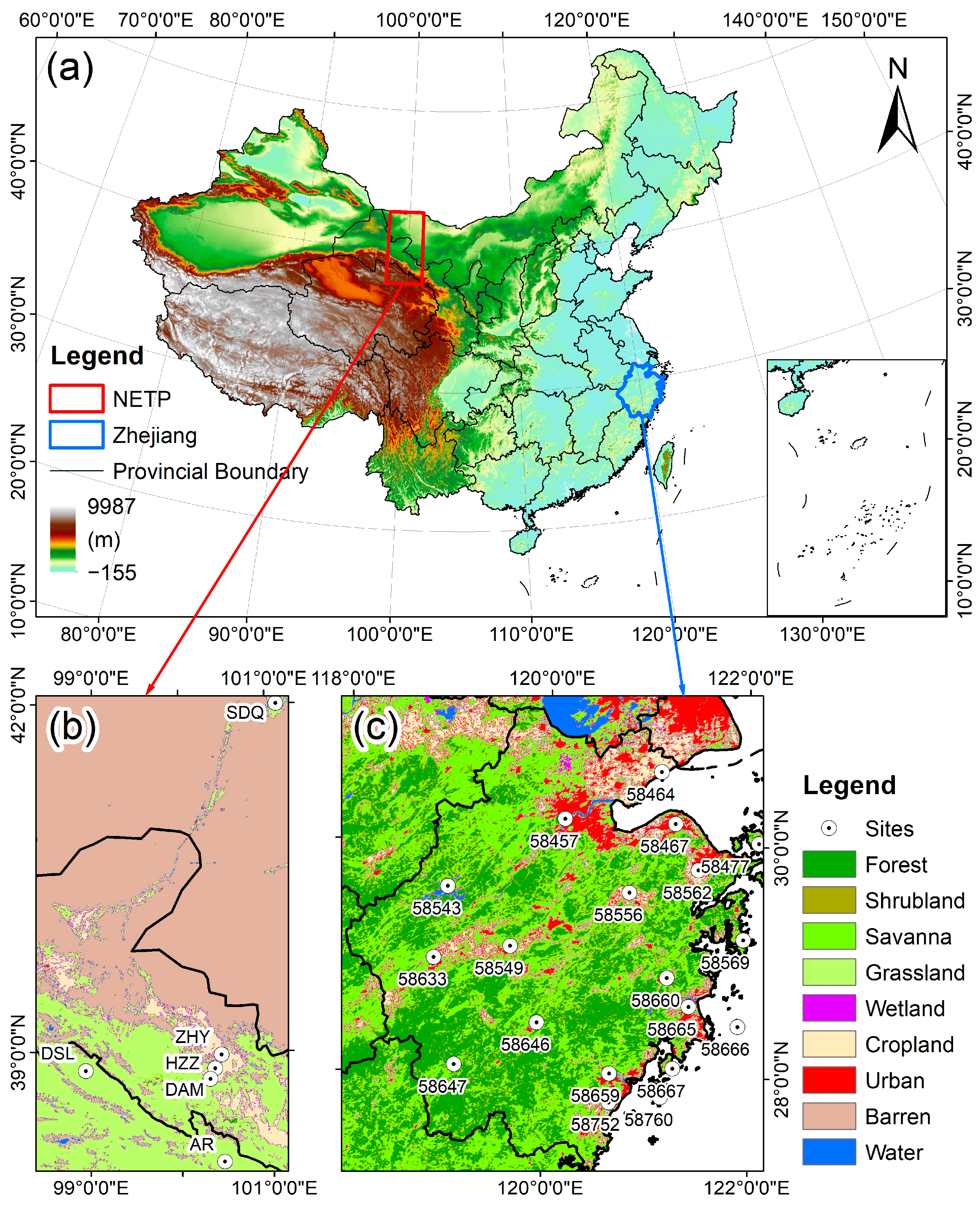
2.1. Study Area

This study selects two study regions to test the downscaling algorithm, one located in the northeastern Tibetan Plateau (NETP) and the other located in Zhejiang Province (Figure 1a).

The NETP study area displays a spatial extent of 98.0–101.4°E and 37.6–42.7°N (Figure 1b), and the elevation range is 5–5495 m. The main land cover types of the NETP are barren land and grassland. In addition, the NETP is often covered with clouds and lacks TIR observations. The complex terrain and cloudy weather conditions make the NETP important for analyzing the DALST. Zhejiang Province located on the southeastern coast of China, which is mainly covered by forest and savanna, while the urban areas are mainly distributed in the coastal zone (see in Figure 1c). The mountainous and hilly terrain, combined with the subtropical monsoon climate, result in a large amount of TIR data loss throughout the year. The distinctly different land cover composition between the NETP and Zhejiang establishes a comparative framework for investigating how surface heterogeneity influences kernel-level feature importance in machine learning frameworks. These characteristics make Zhejiang and the NETP meaningful for testing the DALST.

2.2. Data

2.2.1. Remote Sensing Data

This study utilizes multi-source data from 2017. The all-weather LST product used in this study was obtained by fusing MODIS LST and reanalysis data [10], which was named thermal and reanalysis integrating moderate-resolution spatial-seamless (TRIMS) LST [59]. Since the reanalysis data collected from the Global Land Data Assimilation System (GLDAS) was incorporated in the generation of LST, the reconstructed LST belongs to the all-weather LST. Additionally, the TRIMS LST has a spatial resolution of 1 km, and can be obtained twice a day. When validated against in situ LST measurements collected from 19 ground stations, the root mean square error (RMSE) values were found to range between 0.80 K and 3.68 K, with no obvious differences under different weather conditions.

The MODIS products used in this study include LST (MYD11A1) and NDVI (MOD13Q1). The daily MODIS LSTs are used to obtain the parameters of the annual temperature cycle (ATC) model. The 250 m resolution NDVI product is used to obtain regression kernels after temporal interpolation.

The annual average VIIRS nighttime light (VNL) data with a spatial resolution of 500 m, used to obtain kernels, are collected from https://eogdata.mines.edu/products/vnl/. In addition, the Shuttle Radar Topography Mission digital elevation model (DEM) data (version 4.1) with a resolution of 90 m, obtained from http://www.gscloud.cn/, are also used as kernels.

2.2.2. Reanalysis Data

The daily and monthly averaged ERA5-Land reanalysis products include 2 m SAT, total precipitation (PREP), surface net solar radiation (SSR), and surface net thermal radiation (STR) with a spatial resolution of 0.1°. To address the inherent coarser spatial resolution of the meteorological inputs compared to that of the MODIS LST products (1 km resolution), a thin plate spline (TPS) spatial interpolation technique [60] was implemented. These interpolated reanalysis data are used as meteorologically related kernels.

2.2.3. Ground Measurements

To validate the downscaled LST in the NETP, in situ measurements from the Heihe Watershed Allied Telemetry Experimental Research (HiWATER) experiment were collected as a reference, and the data were downloaded from https://data.tpdc.ac.cn/en/. Six stations were used for validation, including Arou (AR), Daman (DM), Dashalong (DSL), Huazhuaizi (HZZ), Sidaoqiao (SDQ), and Zhangye (ZHY); the land cover types of these sites comprise grassland, cropland, forest, wetland, and desert (see in

Table 1. Details of six ground sites.

Site	Location (°E/°N)	Land Cover	Elevation (m)	Height of Instrument (m)
AR	100.46, 38.05	Alpine meadow	3033	5
DAM	100.37, 38.85	Cropland	1556	12
DSL	98.94, 38.84	Swamp meadow	3739	6
HZZ	100.32, 38.77	Desert	1731	6
SDQ	101.14, 42.00	Mixed forest	873	10
ZHY	100.47, 38.98	Wetland	1460	6

). Moreover, these ground measurements have been used for the validation of various LST products in previous studies [10,61,62,63,64], and their locations are provided in Figure 1b.

In addition, in situ measurements of the 0 cm surface temperature were collected from https://data.cma.cn to evaluate the downscaled LSTs in Zhejiang Province. In situ measurements for a total of 16 sites were used, including those for nine urban sites, four cropland sites, two savanna sites, and one grassland site (Figure 1c). These in situ LSTs were obtained via platinum resistance thermometers, with half of each thermometer horizontally buried in soil, and the estimated LST was reported to exhibit an accuracy of 0.5 K [50]. To achieve the temporal synchronization with the overpass schedules of the TRIMS products, ground-based LST measurements acquired during adjacent observation windows (13:00–14:00 for daytime and 01:00–02:00 for nighttime) were averaged to establish reference datasets corresponding to the 13:30 and 01:30 satellite transit times.

3. Method

3.1. Preprocessing of Regression Kernels

As Zhan et al. [32] illustrated, the regression kernel implies an indicator that connects the LST with the spectral radiance of the surface. Specifically, NDVI is the most often suggested kernel source over vegetation-covered areas [35], and NDBI [28] or the impervious percentage method [65] are often used for urban areas. However, these kernel strategies are applicable for clear sky LST, while the driving factors for cloudy LST are more complex. In this study, I not only use these land surface-related kernels to describe the land surface properties, but I also introduce LST-derived kernels to control the spatial distribution of LSTs and meteorologically related kernels to consider the influence of all-weather condition on LSTs.

The land surface-related kernels used in this study include NDVI, DEM, and VNL. Specifically, NDVI and VNL are more closely related to land cover type, while DEM is more closely related to topographic features. The 90 m resolution DEM data are aggregated to 250 m and 1 km, respectively, by mean aggregation. The VNL images are resampled to 250 m via the nearest neighbor interpolation to serve as kernels at high resolution and are then aggregated to 1 km to serve as kernels at low resolution (see in Figure 2a). To obtain daily NDVI data, I use the changing-weight filter (CWF) method [66] to remove noise from the NDVI images and then use the spline interpolation technique [60] to interpolate the filtered NDVI data (see in Figure 2a). To maintain the shape of the NDVI time series, the CWF method detects the local maximum/minimum points based on a mathematical morphology algorithm and a rule-based decision process, then filters the NDVI time series with a three-point changing-weight filter [66]. In addition, meteorologically related kernels (including PREP, SSR, STR, and SAT), with a resolution of 0.1°, are interpolated to 1 km via the TPS interpolator. Then, I apply the bilinear interpolation to the 1 km data to obtain meteorologically related kernels with a resolution of 250 m.

This study selects the parameters of the ATC model [14] as the LST-derived kernels. The ATC model utilizes a sinusoidal function to simulate cyclical temperature variations, expressed mathematically as follows:

$$T(DOY)=MAST+YAST\cdot \sin ({\displaystyle \frac{2\pi }{365}}\cdot DOY+\theta )$$

(1)

where T is the daily LST, DOY is the day of the year, MAST is the mean annual surface temperature, YAST is the yearly amplitude of the surface temperature, and $\theta$ represents the phase shift. These parameters are obtained from time series LSTs by fitting the ATC model in the IDL platform [15]. The Levenberg−Marquardt minimization scheme is chosen to fit the model because of its robustness in solving nonlinear least squares problems [14,67]. Specifically, I selected MAST and YAST as the LST-derived kernels. Since the resolution of MAST and YAST derived from MODIS LST is 1 km, I use the bilinear interpolation to further obtain the 250 m resolution parameters (see in Figure 2a).

3.2. Basic Assumptions of the Kernel-Driven Method

The kernel-driven downscaling method assumes that the LST and the kernels follow a specific regression relationship, and this relationship is scale-invariant [68]. The regression relationship can be expressed as follows:

$$T_{all}=f(DOY,{\rho }_{Land},{\rho }_{LST},{\rho }_{Met})+\Delta T$$

(2)

where $T_{all}$ is the all-weather LST; f(·) is the function relationship between LST and the kernels; ${\rho }_{Land}$, ${\rho }_{LST}$, and ${\rho }_{Met}$ are the land surface-related kernels, the LST-derived kernels, and the meteorologically related kernels, respectively; $∆T$ is the model residual.

I further add geographical constraint to the above regression relationship; the equation can be expressed as follows:

$$T_{all}=f(DOY,{\rho }_{Land},{\rho }_{LST},{\rho }_{Met},Lon,Lat)+\Delta T$$

(3)

where Lon and Lat are the longitude and latitude of the corresponding pixel. Based on the scale-invariant assumption, I first establish a regression model between the low-resolution LSTs and the kernels, subsequently extrapolating this relationship to high-resolution kernels based on Equation (3). Specifically, the model residual is resampled to 250 m via the bilinear interpolation, then is added to the predicted LST for the final implementation of DALST (see in Figure 2b).

3.3. Incorporation with the Light Gradient-Boosting Machine (LightGBM) Model

To obtain satisfactory downscaling result, the reliable function relationship plays a key role in the downscaling process. Due to the superior nonlinear fitting ability of the LightGBM model and its fast training speed [54], I incorporated it to the Geo-MLKM to obtain a reliable function relationship between the kernels and the LST.

GBDT [69] is a widely used machine learning algorithm which integrates a variety of base classifiers into the new learner. Benefitting from the weighted combination of all the regression trees predictions, GBDT can avoid overfitting. LightGBM is a gradient learning framework based on GBDT [54] which introduces distinct algorithmic innovations compared to those of conventional GBDT frameworks like XGBoost [70]. While XGBoost primarily employs regularization techniques to mitigate overfitting, LightGBM adopts a dual optimization strategy: (1) a histogram-based algorithm (Figure 3) that discretizes continuous features through either a global histogram (single initialization using the full dataset) or a local histogram (node-specific bin adjustment), enabling adaptive handling of heterogeneous data distributions; and (2) a leaf-wise growth method to implement decision tree learning, which searches leaves with the highest branching gain (see in Figure 3) and can reduce ineffective splits, effectively improving the efficiency of the algorithm, contrasting with the level-wise paradigm, which will traverse all the training data during iteration, accordingly increasing the computing cost [54].

As shown in Figure 3, the gradient-based one-side sampling (GOSS) technique is employed to retain all the instances with large gradients and perform random sampling on the instances with small gradients. The exclusive feature bundling (EFB) technique is also be used to reduce the dimensions of the features. By employing the GOSS and EFB techniques, the training speed can be improved without sacrificing accuracy [54]. The successful applications of LightGBM in reconstructing all-sky LSTs [71], downscaling all-sky LSTs [53], and estimating LST from the AMSR2 microwave brightness temperature [58] have revealed the superiority of LightGBM in training large amounts of data with high accuracy and fast computing speed when compared with the results for XGBoost and RF. The LightGBM model training and predicting processes were implemented in Python using the “lightgbm” package.

3.4. Estimation of In Situ LSTs

Because there are few satellite-derived LSTs with resolutions higher than 250 m and which correspond to the acquisition times for all-weather LST products, I mainly use the in situ observations collected from six sites as the reference for evaluating the accuracy of DALST. These six sites provide downward longwave radiation (L_down) and upward longwave radiation (L_up) from four-component radiometers, which can be used to obtain in situ LST. The in situ LST can be calculated as follows:

$$T_s={[{\displaystyle \frac{L_{up}-(1-{\epsilon }_b)\cdot L_{down}}{{\epsilon }_b\cdot \sigma }}]}^{1/4}$$

(4)

where T_s is the in situ LST, $\sigma$ is the Stefan–Boltzmann’s constant (5.67 × 10⁻⁸ W·m⁻²·K⁻⁴), and ${\epsilon }_b$ is the surface broadband emissivity, which can be determined by the land surface emissivities of the MYD11A1 product. The calculation equation is as follows [61,72]:

$${\epsilon }_b=0.2122\cdot {\epsilon }_{29}+0.3859\cdot {\epsilon }_{31}+0.4029\cdot {\epsilon }_{32}$$

(5)

where ${\epsilon }_{29}$, ${\epsilon }_{31}$, and ${\epsilon }_{32}$ are the land surface emissivities of bands 29, 31, and 32 in the MYD11A1 product, respectively, and the missing emissivities under a cloudy sky are linearly interpolated by the clear-sky data.

Here, RMSE, the mean absolute error (MAE), and the determination coefficient (R²) are used to present the training efficiency of the model, and RMSE, MAE, and Pearson’s correlation coefficient (r) are used to quantificationally evaluate the performance of the downscaled LST when compared with the in situ LSTs.

4. Results

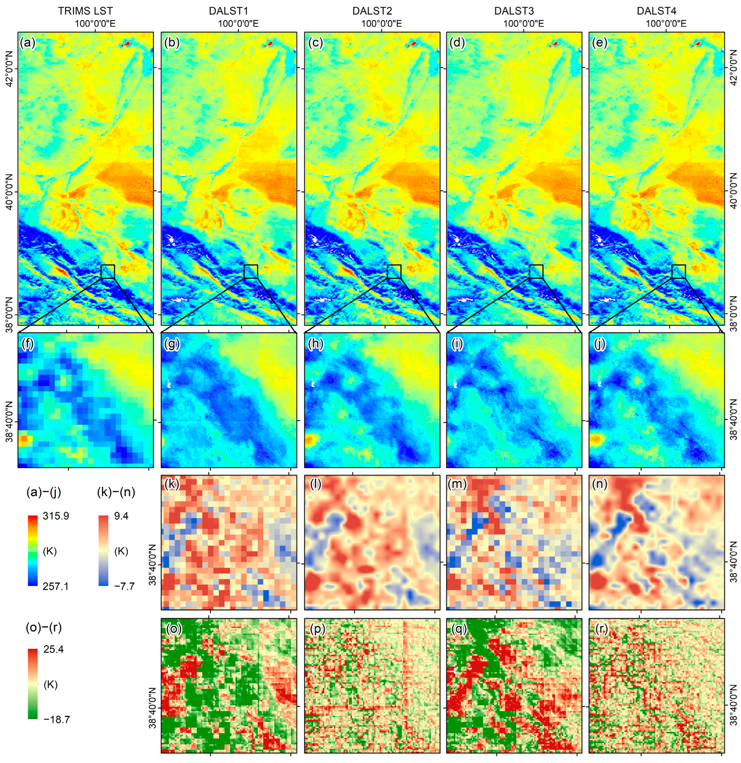
4.1. Spatial Patterns of the Downscaled All-Weather LSTs

This section presents the spatial patterns of the downscaled all-weather LSTs compared with those of the original TRIMS LSTs. Specifically, the downscaled LST, without a model residual, is termed DALST1, and that with the model residual is termed DALST2. In addition, the downscaled results, without geographical constraints (longitude and latitude) and model residuals, are termed DALST3, and the downscaled LST, without geographical constraints but including the model residual, is termed DALST4.

The downscaled results for the NETP are presented in Figure 4. Compared to the TRIMS LST (see in Figure 4f), all downscaled LST products exhibit enhanced spatial details and refined textures (see in Figure 4g–j). Notably, DALST2 and DALST4 effectively preserve the spatial fluctuations observed in TRIMS LST, whereas DALST1 and DALST3 fail to retain critical spatial features, particularly extreme high and low LST values. For instance, DALST2 (Figure 4h) successfully enhances spatial details of TRIMS LST while maintaining temperature extremes, in contrast to DALST1 (Figure 4g), which exhibits a significant loss of high and low temperature signals. This limitation is quantitatively reflected in the LST difference map (DALST1-TRIMS, Figure 4o), showing deviations ranging from −18.7 K to 25.4 K, primarily attributed to the absence of model residual integration in DALST1. Similar artifacts are observed in DALST3 (Figure 4i,q). To mitigate grid artifacts caused by low-resolution residuals, a bilinear-interpolated high-resolution residual (Figure 4l) was generated. Although this interpolation does not introduce additional spatial details compared to those for the original low-resolution residual (Figure 4k), it produces smoother residual fields, thereby enabling the downscaled LST to retain the original temperature variations without sacrificing the extremes. In addition, DALST2, which incorporates longitude and latitude as geographical constraints, demonstrates spatial textures comparable to those of DALST4 (trained without geographical coordinates), suggesting the limited impact of explicit coordinate constraints on texture preservation. A quantitative comparison of their performance will be detailed in Section 4.2.

The spatial patterns of the downscaled nighttime LST in Zhejiang Province are shown in Figure 5, revealing consistency with the NETP observations. Similar to the NETP results, DALST2 and DALST4 exhibit superior spatial detail preservation relative to TRIMS LST when compared to the results for DALST1 and DALST3. Quantitatively, the TRIMS LST ranges from 280.4 to 327.7 K (Figure 5a), while DALST1 exhibits a narrower range of 284.2–320.1 K (Figure 5b). In contrast, DALST2, with model residual, displays a more similar LST range (282.2–323.5 K) to that of the TRIMS LST (see in Figure 5c). Moreover, the DALST2 also retained more high and low temperatures than did the DALST1 (see in Figure 5g,h). This improvement is further evidenced by the spatially smoother and smaller-magnitude discrepancies between DALST2 and the resampled TRIMS LST (Figure 5o,p) when compared to DALST1-TRIMS differences. Compared with DALST3 (see in Figure 5d), DALST1, containing the longitude and latitude in the training model, displays an LST range more similar to that of the TRIMS LST; however, this difference has been reduced by the added model residual (see in Figure 5e). The lost high and low temperatures of DALST3 can also be filled by the DALST4 (see in Figure 5i,j). These findings collectively demonstrate that (1) geographical constraints (longitude/latitude) enhance model accuracy; (2) model residual correction significantly refines downscaled LST fidelity, particularly in regards to extreme temperature retention.

These results indicate that DALST can well-enhance the spatial details of the low-resolution LST, and the model residual should be taken seriously in the DALST.

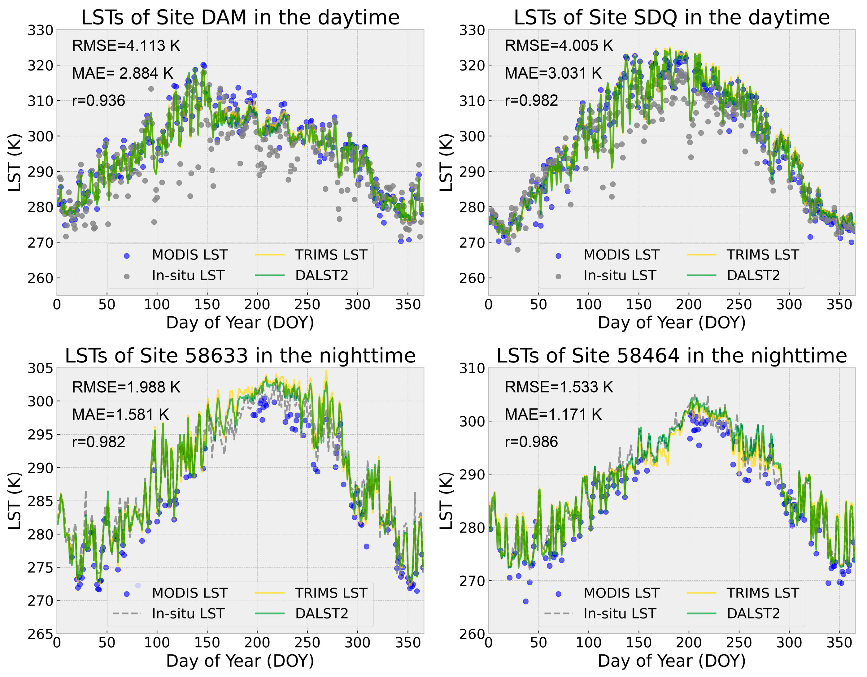
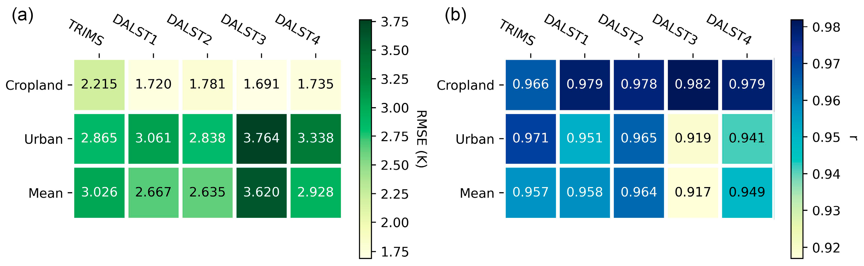
4.2. Quantitative Evaluation of the Downscaled All-Weather LSTs

This section uses the in situ LSTs from six stations to quantificationally evaluate the performance of DALST in the NETP, and uses the in situ LSTs of 16 sites to evaluate the performance of DALST in Zhejiang. Specifically, due to the significant difference between the LSTs collected by the platinum resistance thermometers and those obtained by remote sensing images in the daytime [50], this study only used nighttime in situ LSTs to evaluate the performance of DALST in Zhejiang.

To evaluate the performance of the DALST, I separately calculated the accuracy of DALST under clear and cloudy sky conditions. As shown in Figure 6a, the daytime LSTs under clear skies demonstrate significantly higher downscaling accuracy compared to those under cloudy conditions. Specifically, the clear-sky results yield an RMSE of 2.865 K, an MAE of 2.266 K, and a correlation coefficient (r) of 0.978, whereas the cloudy-sky performance degrades to an RMSE of 6.535 K, an MAE of 5.190 K, and an r of 0.880. The lower accuracy of the daytime DALST under cloudy skies compared to clear-sky conditions may be attributed to the potential underestimation in the in situ observations under cloudy skies. This conclusion is supported by the moderate performance metrics of the TRIMS LST under cloudy conditions when validated against the ground measurements, demonstrating an RMSE of 6.609 K, an MAE of 5.270 K, and an r value of 0.879. In the nighttime, this difference between clear and cloudy skies is not as obvious as that in the daytime. As shown in Figure 6b,c, in the NETP and Zhejiang, both clear and cloudy skies present satisfactory accuracies, whose r values are both larger than 0.94. In Zhejiang, the RMSEs of the clear and cloudy skies are closer, i.e., the RMSEs are 2.233 K and 2.766 K for clear and cloudy skies, respectively. These differences may be due to the smaller temperature fluctuation in the nighttime than that in the daytime. Specifically, there is a stable boundary layer at night, whose function is similar to that of the cloud-topped planetary boundary layers (PBL), thus making the nighttime temperature difference smaller between clear and cloudy skies.

To present the consistency of the DALST and TRIMS LST, the temporal patterns of the DALST and TRIMS LST for specific sites are provided. As shown in Figure 7, for sites DAM and SDQ, the DALST exhibits almost the same temporal patterns as those derived from the TRIMS LST; it also well captured the temporal variations in MODIS LST, as the r values compared to the in situ LST are both larger than 0.93. At night in Zhejiang, the DALST not only displays high consistency with TRIMS LST and MODIS LST, but also exhibits high similarity to in situ LST. The RMSEs are both smaller than 2.0 K, and the r values are up to 0.98. These results present the satisfactory downscaling results of DALST.

To further compare the DALST with the TRIMS LST, the accuracies of the DALST and TRIMS LST when referenced to six stations in the NETP are provided. As shown in Figure 8a,b, in the daytime, DALST1 shows the best accuracies, with a lower RMSE and a higher r value except, in site AR. As for the results presented in Section 4.1, the DALST1 without model residual has lost both the high and low temperatures compared to the results for TRIMS LST. The slightly higher accuracy of DALST1 compared with DALST2 in site AR may be caused by the outliers of the site [61]. In addition, DALST2 shows best accuracies for site DAM and site HZZ, with lower RMSE and higher r values. However, DALST 4 displays the best accuracies for sites DSL, SDQ, and ZHY. The daytime average improvement for DALST2 compared to TRIMS LST is 0.05 K, while that of DALST4 is 0.15 K. As shown in Figure 8c,d, in the nighttime, DALST1 displays the best accuracies for sites AR, DAM, HZZ, and SDQ, while DALST2 shows the best accuracies for sites DSL and ZHY, respectively. The improvement in the DALST when compared with the results for the TRIMS LST is even smaller than that in the daytime, which is due to the relatively homogenous temperature fluctuation at night. Furthermore, the p-values for both TRIMS LST and DALST2 exceeded 0.05 during nocturnal measurements (p = 0.997 and p = 0.952, respectively), indicating no statistically significant associations.

The validation results based on 16 in situ stations in Zhejiang Province (Figure 9) demonstrate distinct performance patterns among the downscaled LST products. Statistical results indicate that the p value of all LSTs is smaller than 0.05, except for DALST3 (p = 0.139). Both DALST1 and DALST2 exhibit significantly lower RMSE values and higher correlation coefficients (r) than does TRIMS LST, with particularly notable improvements in cropland areas. Specifically, the RMSE reductions for DALST1 and DALST2 reach 0.495 K and 0.434 K in croplands (including four sites), respectively. In contrast, the superiority of the DALST method is less pronounced in urban areas (including nine sites), where DALST2 achieves only a marginally lower RMSE than does TRIMS LST. Furthermore, DALST3 and DALST4 (models without geographical constraints) exhibit significantly lower accuracy than do DALST1 and DALST2, particularly in urban areas, demonstrating the critical role of geographical constraints in enhancing model performance. By incorporating model residuals, the RMSE of DALST4 is reduced to 2.928 K, highlighting that residual correction effectively addresses limitations in model training.

The above temporal variations in LSTs and the quantitative comparisons indicate that the DALST has well-followed the temperature variation in TRIMS LST and MODIS LST when adding spatial details to the low-resolution LSTs. Although DALST1 shows slightly higher accuracies in some sites, this may be because these sites are located in homogenous land surfaces that do not contain the extreme high and low temperatures presented in Figure 4. Combined with the spatial comparisons with TRIMS LST, DALST2 with a model residual can better maintain the temperature texture than can that without the model residual.

5. Discussion

5.1. Model Performance of Different Kernel Combinations

To explore the model performance of the input kernels, models with different kernel combinations were trained. I also used the XGBboost model [70] to train these kernel combinations in Python 3.9 to enable comparisons with the LightGBM model. Specifically, the dataset was partitioned using a stratified random sampling approach with a 70:30 training–testing ratio across both study regions. In the NETP, the model training incorporated approximately 3.2 × 10⁶ spatially representative samples, while validation utilized 1.3 × 10⁶ independent test samples. For the Zhejiang Province analysis, this geospatial cross-validation framework employed 4.0 × 10⁶ training samples and 1.7 × 10⁶ testing samples., The accuracies of training and testing with different kernel combinations are provided in

Table 2. Model training accuracies.

Model	Training			Test
	RMSE	MAE	R2	RMSE	MAE	R2
Light (ρMet)	1.405	1.016	0.983	1.419	1.024	0.983
Light (ρLST)	1.823	1.307	0.974	1.838	1.316	0.973
Light (ρLST, ρMet)	1.305	0.942	0.986	1.321	0.951	0.985
Light (ρland)	1.866	1.347	0.972	1.880	1.356	0.972
Light (ρLand, ρMet)	1.353	0.984	0.985	1.369	0.994	0.984
Light (ρLand, ρLST)	1.840	1.322	0.973	1.856	1.332	0.973
Light (ρLand, ρLST, ρMet)	1.298	0.940	0.986	1.316	0.950	0.986
XGB (ρMet)	2.578	1.954	0.946	2.578	1.954	0.946
XGB (ρLST)	2.545	1.946	0.949	2.544	1.946	0.949
XGB (ρLST, ρMet)	2.147	1.606	0.964	2.147	1.606	0.964
XGB (ρland)	2.731	2.101	0.942	2.729	2.100	0.942
XGB (ρLand, ρMet)	2.321	1.748	0.958	2.321	1.747	0.958
XGB (ρLand, ρLST)	2.567	1.966	0.948	2.566	1.965	0.948
XGB (ρLand, ρLST, ρMet)	2.148	1.606	0.964	2.148	1.606	0.964

. The accuracies of training data are usually slightly higher than those of test data. The model trained with land surface-related kernels (i.e., NDVI, DEM, and VNL) tend to exhibit the poorest performance, e.g., the RMSEs of the training data and test data are both larger than 1.86 K. The model trained with LST-derived kernels (i.e., MAST and YAST) performs slightly better than that trained with land surface-related kernels. The model trained with meteorologically related kernels (i.e., PREP, SSR, STR, and SAT) performs much better than the other two types of kernels, e.g., the RMSEs of the training data and the test data are 1.405 K and 1.419 K, respectively. Therefore, when the meteorologically related kernels were combined with the land surface-related kernels or the LST-derived kernels, the model performance was significantly improved. For example, when the LightGBM model is trained with land surface-related kernels and meteorologically related kernels, the RMSE of train data is 1.353 K, which has been reduced by about 0.5 K compared with that trained with land surface-related kernels. When all three kinds of kernels are used, the model performance is the best, the RMSEs of which are 1.298 K and 1.316 K for train data and test data, respectively. In addition, the model trained with the combination of LST-derived kernels and meteorologically related kernels exhibits similar training accuracy to that of the model trained with all kernels, the RMSEs of which are 1.305 K and 1.321 K for training data and test data, respectively. The kernel combinations trained via the XGBoost model show similar performance to that of those trained via the LightGBM model; however, the accuracy is much lower, which is similar to the results of a previous study [58].

The kernel importance derived from the model training is provided in Figure 10. Here, I trained these data separately to show the variation in kernel importance according to different study regions. As shown in Figure 10, the smallest importance is found in NDVI, with an average value of 2.237%. Specifically, the NDVI importance is slightly larger in NETP than in Zhejiang; that is because NDVI is more suitable for use in a homogenous landscape [35,36]. In addition, the VNL importance is obviously larger in Zhejiang than in the NETP, since nightlight data can well-map the urban extent [73]. Except for DOY and longitude and latitude, the largest importance is for SAT, with an average value of 11.433%, and the largest SAT importance occurs in the nighttime NETP, with a value of 12.32%. The larger kernel importance for SAT is because the air temperature is highly related to the surface temperature [74]. There are importance differences between land surface-related kernels and other kernels. The average importance of land surface-related kernels, LST-derived kernels, and meteorologically related kernels is 4.493%, 6.598%, and 8.222%, respectively. The higher importance of the meteorologically related kernels compared with the land surface-related kernels (e.g., NDVI) corroborates the findings of Zhang et al. [8]. That is because meteorologically related kernels, like surface net solar radiation (SSR) and surface net thermal radiation (STR), can represents the radiation energy input, which determines the rise or fall of LST [8].

The above results indicate the greater importance of LST-derived kernels and meteorologically related kernels compared with that of land surface-related kernels. Although the land surface-related kernels make a smaller contribution to the improvement of model training, they display more abundant spatial details than the resampled LST-derived kernels and the meteorologically related kernels. Therefore, this study combined these land surface-related kernels to further enhance the spatial resolution of all-weather LSTs.

5.2. Effect of Geographical Constraints on Model Training

To explore the effects of geographical constraints on model training, I trained a LightGBM model, without latitude and longitude, as the model without geographical constraints. As shown in Figure 11, the model with geographical constraints exhibits improved training accuracy, with the RMSE reduced by 0.16 K and the R² increased by 0.004. The improvement in geographical constraints is not significant in the training model. In addition, the model residual incorporated in the DALST can also make up for the poorer performance of the training model, thereby improving the accuracy of DALST. However, the slightly higher accuracy of the DALST with geographical constraints compared with that without geographical constraints at night reveals that the geographical constraints can certainly help to improve the performance of DALST (see Section 4.2). Compared with the GWR [41] and GTWR [42] models, which consider the spatial heterogeneity by applying geographically varying regression coefficients in regression, adding the spatial locations to Geo-MLKM in the training process is an easier solution.

5.3. Effects of Weather Conditions on Model Training

To further explore the performance of kernels under different weather conditions, monthly averaged data with different missing data rates were trained separately. Specifically, I compiled the statistics for the percentage of valid monthly aggregated LSTs data for one month. The datasets were split according to the percentage of clear days in a month and were classified into three groups (i.e., clear sky, cloudy sky, and heavily clouded) according to the tripartite thresholds (see in Figure 12a). Then, the LightGBM model was trained separately based on these classified LSTs, and the kernel importance was presented accordingly. The experimental configuration employed substantial sample sizes to ensure statistical robustness. For the NETP, about 300,000 training samples, with 150,000 test samples, were used for each separate condition; for Zhejiang, about 400,000 training samples, with 180,000 test samples, were used for each separate condition.

As shown in Figure 12a, the black and red dotted lines appear in the locations where the values of the percentage of clear days are the three equinoxes, and the percentages of clear days in one month follow the Gaussian distribution. In Zhejiang, the valid data make up less than 50% of the total, of which the mean values of the percentage of clear days in one month are all less than 30%. Compared with Zhejiang, the NETP exhibits more clear-sky LSTs, and the mean values of the percentage of clear days are 54.9% and 64.1% in the daytime and nighttime, respectively.

As shown in Figure 12b,c, when trained using all data, except for location information, the LST-derived kernels display the greatest importance both during the day and at night. In the NETP region, MAST is the most important regression kernel under all weather conditions, and the land surface-related kernels and meteorologically related kernels display nearly equal importance (see in Figure 12b). In both regions, the kernel importance of the land surface-related kernels increases as the clear days increase in one month; in contrast, the kernel importance of the meteorologically related kernels increases as the clear days reduce (see in Figure 12c).

Comparative analysis reveals distinct kernel contribution patterns: land surface-related kernels demonstrate significantly higher predictive importance under clear-sky conditions, while meteorologically related kernels exhibit the opposite trend, showing enhanced explanatory power under cloud-affected scenarios.

5.4. Advantages and Possible Issues of DALST via the Geo-MLKM

Tested with data in the NETP and Zhejiang Province, the Geo-MLKM applied for implementing DALST presents the following advantages.

First, the kernel-driven method obtains spatial details from various kernels, which can reduce the DALST’s dependency on the single-type regression kernel. When trained with the LightGBM model, the lower importance of the land surface-related kernels reveals that implementing DALST with only land surface-related kernels may be insufficient, producing larger errors (see in Section 5.1). Although the resolution of both LST-derived kernels and meteorologically related kernels is relatively low, and cannot fully enhance the spatial information of all-weather LST, the integrated utilization of all three types of kernels enables the comprehensive extraction of spatial details through land surface-related kernels, while exploiting the strong correlation between LSTs and the other two types of kernels to guide the LST distribution. The more abundant spatial details presented by the downscaled LST (see in Section 4.1) and the quantitative evaluated results obtained from in situ observations (see in Section 4.2) have proven the effectiveness of the combinations of various kernels.

Second, the LightGBM model applied in the DALST makes it possible to generate a large number of high-resolution all-weather LSTs with high efficiency and satisfactory accuracy. Specifically, the experiment was implemented in Windows 10, the corresponding processor comprises a 12th Gen Intel(R) Core (TM) i9-12900, and the Graphics card is NVIDIA GeForce RTX 3080. When training regression models on daily datasets (about 3.2 × 10⁶ samples) in the NETP region, LightGBM demonstrated superior computational efficiency, requiring approximately 10 min to complete model training. In contrast, the RF implementation necessitated a substantially longer training duration of one hour. While XGBoost exhibits comparable computational efficiency to that of LightGBM within the specific sample size ranges (e.g., 3.2 × 10⁶ samples), LightGBM demonstrates markedly accelerated training performance on large-scale datasets due to its optimized GPU-accelerated architecture, which enables efficient parallel computation for high-dimensional data processing [54]. In addition, the experiment in Section 5.1 reveals that LightGBM displays better accuracy than that of XGBoost. These characteristics of LightGBM make it possible to implement DALST over a larger study areas. Existing LST reconstruction work based on the LightGBM model [58] also proves its prospects for use with DALST at large scales.

The above advantages reveal the possibility of using Geo-MLKM to generate a large number of high-resolution all-weather LSTs. However, there are still some issues that might affect the performance of DALST in future applications.

On the one hand, the effect of the resolution difference between various kernels on the DALST should be considered. The kernels in this study mainly include land surface-related kernels, LST-derived kernels, and meteorologically related kernels. Specifically, the resolution of the land surface-related kernels is higher than that of meteorologically related kernels, which are obtained from the reanalysis data with a resolution of 0.1°. The LST-derived kernels are resampled to 250 m via bilinear interpolation, which will lose many spatial details. These kernels with lower spatial resolution offer limited spatial details, resulting in a smoothed downscaled LST. To mitigate the impact of coarser-resolution meteorologically related kernels on downscaled LST, integrating high-density weather station observations can enhance the resolution of these kernels. Additionally, incorporating more fine-resolution land surface-related kernels can improve the spatial details of downscaled LST.

On the other hand, the effect of uncertainties of the input all-weather LST products on the DALST should also be considered. This study selects the TRIMS LST, which is derived from the fusion of MODIS LST and reanalysis data, with the RMSE ranging from 0.80 K to 3.68 K [59]. Compared with the available all-weather LST product produced by Xu et al. [12], this product is more mature, with acceptable accuracy. Despite this, TRIMS LST still exerts grid effects on some images, which can then be transmitted to the DALST result. Since this study only used the bilinear interpolation to process the model residual for simplicity, some texture issues existing in the original LST products have not been well-solved. Traditional residual correction processes, like kriging interpolation [38,41,75], cubic interpolation [49], and direct addition without interpolation [36], cannot avoid this issue. Establishing kernel relationships with LST differences [49] instead of raw LST values could alleviate texture deficiencies in input products, since the LST difference variation is smaller than that of the LST. Further improving the quality of the all-weather LST products can help to solve this problem. In addition, obtaining the spatial details from other data, rather than from all-weather LST, can make the DALST less reliant on the image quality of all-weather LST.

5.5. Comparison with Previous DLST Studies

Compared with DLST using the kernel-driven method under clear skies [35,65], the DALST adopting the Geo-MLKM in this study not only uses high-resolution visible and near-infrared (VNIR) data as kernels to construct relationship between kernels and LSTs but also uses meteorological data with low resolution as kernels. The meteorological data can support the reflection of LSTs under clear and cloudy skies, guiding the overall temperature over a large region, but the low-resolution meteorological data cannot provide abundant spatial details for all-weather LSTs. Therefore, the high-resolution land surface-related kernels, providing spatial details, are used to replace them. Compared with the SED algorithm proposed by Dong et al. [49], which incorporates LSTs at two times in one day and downscales the LST differences via the RF method, the proposed method directly downscales the LST by training the relationship between daily LSTs (collected over one year at the same local solar time) and kernels and is more applicable for large-area downscaling, since the LightGBM is superior to the RF method due to its excellent nonlinear fitting ability and its fast training speed [54]. Inspired by Dong et al. [49], the proposed method can further consider building relationship between the LST difference and the kernels to improve accuracy.

Compared with DLST under cloudy skies, this study implemented the DALST based on the available all-weather LST product rather than on PMW or reanalysis data. The spatial resolution of LSTs obtained from PMW or reanalysis data is coarser than 1 km [7,51], and the inclusion of fewer spatial details can magnify the difficulty of DALST when the target resolution is quite high. Huang et al. [53] implemented the DALST based on an all-weather LST product using the LightGBM model. However, their study uses only land surface-related kernels (including elevation, slope, aspect, land cover type, vegetation index, surface reflectivity, and snow index) for downscaling, without considering the impact of LST-derived kernels and meteorologically related kernels. Compared with the DALST implemented by Huang et al. [53], this study has investigated the kernel importance of DALST and found that the meteorologically related kernels and LST-derived kernels exert a greater effect on the DALST than do the land surface-related kernels in most cases, which reveals the indispensability of these kernels. The accuracy improvement (RMSE_TRIMS = 3.026 K vs. RMSE_DALST = 2.635 K) tested in Zhejiang reaches 0.391 K, which is higher than that of Huang et al. [53] (ΔRMSE = 0.25 K). In addition, the combination with different kernels helps to reduce the dependency of DALST on VNIR data, especially under cloudy conditions when the land surface-related kernels display lower importance.

The above comparisons with previous DLST studies have proven the effectiveness of DALST via the Geo-MLKM method. The evaluation of DALST with various kernels indicates the superiority and potential for DALST to generate a large number of high-resolution all-weather LSTs via Geo-MLKM.

6. Conclusions

This study implements DALST via the Geo-MLKM and investigates the importance of different kernels. The LightGBM model incorporated in DALST not only maintains the high accuracy of model training but also improves the operating efficiency in dealing with a large number of datasets. The application of different types of kernels further reduces DALST’s dependence on a single type of kernel. These characteristics make it possible for the Geo-MLKM to produce a large number of high-resolution all-weather LSTs at large scales.

The DALST was tested in the northeastern Tibetan Plateau (NETP) region and Zhejiang Province. The spatial patterns of downscaled all-weather LSTs with residual correction indicate that DALST can enhance the spatial details, while maintaining the temperature fluctuations. The temporal patterns reveal a high correspondence of the downscaled LST to the TRIMS LST and MODIS LST. When compared with the in situ LSTs, the downscaled LST exhibits satisfactory accuracy in the NETP, i.e., the r values are 0.933 and 0.969 for the daytime and nighttime, respectively. The RMSEs are 4.885 K for the daytime and 3.141 K for the nighttime. Tested in Zhejiang, the RMSE of the downscaled LST is 2.635 K, which is reduced by 0.391 K compared with that of the TRIMS LST. Comparisons with different kernel combinations reveal the different roles of kernels, i.e., land surface-related kernels are used to enrich the spatial details of LSTs, and the roles of LST-derived kernels and meteorologically related kernels are to ensure that the predictions are within the reasonable range. Compared with the XGBoost model, the LightGBM model incorporated in this study show a better performance in the model training process. In addition, the geographical constraint has also improved the model performance.

The DALST implemented in this study has generated daily 250 m resolution all-weather LSTs in the NETP and Zhejiang, with satisfactory quality. Future research may consider generating more LSTs with a higher resolution at a larger scale for various environmental studies, which will require enhanced computational efficiency through optimized algorithms and advanced parallel computing architectures to handle the exponentially increasing data volumes associated with finer spatial resolutions and larger geographical coverage.

References

1. Oliveira, A.; Lopes, A.; Niza, S.; Soares, A. An urban energy balance-guided machine learning approach for synthetic nocturnal surface urban heat island prediction: A heatwave event in Naples. Sci. Total Environ. 2022, 805, 150130. [Google Scholar] [CrossRef] [PubMed]
2. Li, Y.; Li, Z.L.; Wu, H.; Zhou, C.; Liu, X.; Leng, P.; Yang, P.; Wu, W.; Tang, R.; Shang, G.F.; et al. Biophysical impacts of earth greening can substantially mitigate regional land surface temperature warming. Nat. Commun. 2023, 14, 121. [Google Scholar] [CrossRef] [PubMed]
3. Wu, Y.; Wen, B.; Li, S.; Gasparrini, A.; Tong, S.; Overcenco, A.; Urban, A.; Schneider, A.; Entezari, A.; Vicedo-Cabrera, A.M.; et al. Fluctuating temperature modifies heat-mortality association around the globe. Innovation 2022, 3, 100225. [Google Scholar] [CrossRef] [PubMed]
4. Yan, H.; Zarekarizi, M.; Moradkhani, H. Toward improving drought monitoring using the remotely sensed soil moisture assimilation: A parallel particle filtering framework. Remote Sens. Environ. 2018, 216, 456–471. [Google Scholar] [CrossRef]
5. Duan, S.-B.; Li, Z.-L.; Leng, P. A framework for the retrieval of all-weather land surface temperature at a high spatial resolution from polar-orbiting thermal infrared and passive microwave data. Remote Sens. Environ. 2017, 195, 107–117. [Google Scholar] [CrossRef]
6. Wu, P.; Yin, Z.; Zeng, C.; Duan, S.-B.; Gottsche, F.-M.; Ma, X.; Li, X.; Yang, H.; Shen, H. Spatially continuous and high-resolution land surface temperature product generation: A review of reconstruction and spatiotemporal fusion techniques. IEEE Geosci. Remote Sens. Mag. 2021, 9, 112–137. [Google Scholar] [CrossRef]
7. Long, D.; Yan, L.; Bai, L.; Zhang, C.; Li, X.; Lei, H.; Yang, H.; Tian, F.; Zeng, C.; Meng, X.; et al. Generation of MODIS-like land surface temperatures under all-weather conditions based on a data fusion approach. Remote Sens. Environ. 2020, 246, 111863. [Google Scholar] [CrossRef]
8. Zhang, H.; Tang, B.-H.; Li, Z.-L. A practical two-step framework for all-sky land surface temperature estimation. Remote Sens. Environ. 2024, 303, 113991. [Google Scholar] [CrossRef]
9. Zhu, X.; Duan, S.-B.; Li, Z.-L.; Wu, P.; Wu, H.; Zhao, W.; Qian, Y. Reconstruction of land surface temperature under cloudy conditions from Landsat 8 data using annual temperature cycle model. Remote Sens. Environ. 2022, 281, 113261. [Google Scholar] [CrossRef]
10. Zhang, X.; Zhou, J.; Liang, S.; Wang, D. A practical reanalysis data and thermal infrared remote sensing data merging (RTM) method for reconstruction of a 1-km all-weather land surface temperature. Remote Sens. Environ. 2021, 260, 112437. [Google Scholar] [CrossRef]
11. Zhang, T.; Zhou, Y.; Zhu, Z.; Li, X.; Asrar, G.R. A global seamless 1 km resolution daily land surface temperature dataset (2003–2020). Earth Syst. Sci. Data 2022, 14, 651–664. [Google Scholar] [CrossRef]
12. Xu, S.; Cheng, J.; Zhang, Q. A random forest-based data fusion method for obtaining all-weather land surface temperature with high spatial resolution. Remote Sens. 2021, 13, 2211. [Google Scholar] [CrossRef]
13. Ke, L.; Ding, X.; Song, C. Reconstruction of time-series MODIS LST in central Qinghai-Tibet plateau using geostatistical approach. IEEE Geosci. Remote Sens. Lett. 2013, 10, 1602–1606. [Google Scholar] [CrossRef]
14. Bechtel, B. A new global climatology of annual land surface temperature. Remote Sens. 2015, 7, 2850–2870. [Google Scholar] [CrossRef]
15. Xia, H.; Chen, Y.; Gong, A.; Li, K.; Liang, L.; Guo, Z. Modeling daily temperatures via a phenology-based annual temperature cycle model. IEEE J. Sel. Top. Appl. Earth Obs. Remote Sens. 2021, 14, 6219–6229. [Google Scholar] [CrossRef]
16. Sun, L.; Chen, Z.; Gao, F.; Anderson, M.; Song, L.; Wang, L.; Hu, B.; Yang, Y. Reconstructing daily clear-sky land surface temperature for cloudy regions from MODIS data. Comput. Geosci. 2017, 105, 10–20. [Google Scholar] [CrossRef]
17. Jin, M. Interpolation of surface radiative temperature measured from polar orbiting satellites to a diurnal cycle: 2. Cloudy-pixel treatment. J. Geophys. Res. Atmos. 2000, 105, 4061–4076. [Google Scholar] [CrossRef]
18. Lu, L.; Venus, V.; Skidmore, A.; Wang, T.; Luo, G. Estimating land-surface temperature under clouds using MSG/SEVIRI observations. Int. J. Appl. Earth Obs. Geoinf. 2011, 13, 265–276. [Google Scholar] [CrossRef]
19. Yu, W.; Ma, M.; Wang, X.; Tan, J. Estimating the land-surface temperature of pixels covered by clouds in MODIS products. J. Appl. Remote Sens. 2014, 8, 083525. [Google Scholar] [CrossRef]
20. Fu, P.; Xie, Y.; Weng, Q.; Myint, S.; Meacham-Hensold, K.; Bernacchi, C. A physical model-based method for retrieving urban land surface temperatures under cloudy conditions. Remote Sens. Environ. 2019, 230, 111191. [Google Scholar] [CrossRef]
21. Semmens, K.A.; Anderson, M.C.; Kustas, W.P.; Gao, F.; Alfieri, J.G.; McKee, L.; Prueger, J.H.; Hain, C.R.; Cammalleri, C.; Yang, Y.; et al. Monitoring daily evapotranspiration over two California vineyards using Landsat 8 in a multi-sensor data fusion approach. Remote Sens. Environ. 2016, 185, 155–170. [Google Scholar] [CrossRef]
22. Shen, H.; Huang, L.; Zhang, L.; Wu, P.; Zeng, C. Long-term and fine-scale satellite monitoring of the urban heat island effect by the fusion of multi-temporal and multi-sensor remote sensed data: A 26-year case study of the city of Wuhan in China. Remote Sens. Environ. 2016, 172, 109–125. [Google Scholar] [CrossRef]
23. Xia, H.; Chen, Y.; Song, C.; Li, J.; Quan, J.; Zhou, G. Analysis of surface urban heat islands based on local climate zones via spatiotemporally enhanced land surface temperature. Remote Sens. Environ. 2022, 273, 112972. [Google Scholar] [CrossRef]
24. Chejarla, V.R.; Maheshuni, P.K.; Mandla, V.R. Quantification of LST and CO2 levels using landsat-8 thermal bands on urban environment. Geocarto Int. 2015, 31, 913–926. [Google Scholar] [CrossRef]
25. Fattah, M.A.; Morshed, S.R.; Morshed, S.Y. Impacts of land use-based carbon emission pattern on surface temperature dynamics: Experience from the urban and suburban areas of Khulna, Bangladesh. Remote Sens. Appl. Soc. Environ. 2021, 22, 100508. [Google Scholar] [CrossRef]
26. Ma, J.; Shen, H.; Wu, P.; Wu, J.; Gao, M.; Meng, C. Generating gapless land surface temperature with a high spatio-temporal resolution by fusing multi-source satellite-observed and model-simulated data. Remote Sens. Environ. 2022, 278, 113083. [Google Scholar] [CrossRef]
27. Zhao, Y.; Huang, B.; Song, H. A robust adaptive spatial and temporal image fusion model for complex land surface changes. Remote Sens. Environ. 2018, 208, 42–62. [Google Scholar] [CrossRef]
28. Xia, H.; Chen, Y.; Li, Y.; Quan, J. Combining kernel-driven and fusion-based methods to generate daily high-spatial-resolution land surface temperatures. Remote Sens. Environ. 2019, 224, 259–274. [Google Scholar] [CrossRef]
29. Pu, R.; Bonafoni, S. Thermal infrared remote sensing data downscaling investigations: An overview on current status and perspectives. Remote Sens. Appl. Soc. Environ. 2023, 29, 100921. [Google Scholar] [CrossRef]
30. Wang, X.; Zhong, L.; Ma, Y. Estimation of 30 m land surface temperatures over the entire Tibetan Plateau based on Landsat-7 ETM+ data and machine learning methods. Int. J. Digit. Earth 2022, 15, 1038–1055. [Google Scholar] [CrossRef]
31. Bian, Z.; Roujean, J.L.; Fan, T.; Dong, Y.; Hu, T.; Cao, B.; Li, H.; Du, Y.; Xiao, Q.; Liu, Q. An angular normalization method for temperature vegetation dryness index (TVDI) in monitoring agricultural drought. Remote Sens. Environ. 2023, 284, 113330. [Google Scholar] [CrossRef]
32. Zhan, W.; Chen, Y.; Zhou, J.; Wang, J.; Liu, W.; Voogt, J.; Zhu, X.; Quan, J.; Li, J. Disaggregation of remotely sensed land surface temperature: Literature survey, taxonomy, issues, and caveats. Remote Sens. Environ. 2013, 131, 119–139. [Google Scholar] [CrossRef]
33. Xia, H.; Chen, Y.; Quan, J.; Li, J. Object-based window strategy in thermal sharpening. Remote Sens. 2019, 11, 634. [Google Scholar] [CrossRef]
34. Gao, L.; Zhan, W.; Huang, F.; Quan, J.; Lu, X.; Wang, F.; Ju, W.; Zhou, J. Localization or globalization? Determination of the optimal regression window for disaggregation of land surface temperature. IEEE Trans. Geosci. Remote Sens. 2017, 55, 477–490. [Google Scholar] [CrossRef]
35. Agam, N.; Kustas, W.P.; Anderson, M.C.; Li, F.; Neale, C.M.U. A vegetation index based technique for spatial sharpening of thermal imagery. Remote Sens. Environ. 2007, 107, 545–558. [Google Scholar] [CrossRef]
36. Kustas, W.P.; Norman, J.M.; Anderson, M.C.; French, A.N. Estimating subpixel surface temperatures and energy fluxes from the vegetation index–radiometric temperature relationship. Remote Sens. Environ. 2003, 85, 429–440. [Google Scholar] [CrossRef]
37. Jeganathan, C.; Hamm, N.A.S.; Mukherjee, S.; Atkinson, P.M.; Raju, P.L.N.; Dadhwal, V.K. Evaluating a thermal image sharpening model over a mixed agricultural landscape in India. Int. J. Appl. Earth Obs. Geoinf. 2011, 13, 178–191. [Google Scholar] [CrossRef]
38. Wang, S.; Luo, X.; Peng, Y. Spatial downscaling of MODIS land surface temperature based on geographically weighted autoregressive model. IEEE J. Sel. Top. Appl. Earth Obs. Remote Sens. 2020, 13, 2532–2546. [Google Scholar] [CrossRef]
39. Yang, G.; Pu, R.; Zhao, C.; Huang, W.; Wang, J. Estimation of subpixel land surface temperature using an endmember index based technique: A case examination on aster and MODIS temperature products over a heterogeneous area. Remote Sens. Environ. 2011, 115, 1202–1219. [Google Scholar] [CrossRef]
40. Bechtel, B.; Zakšek, K.; Hoshyaripour, G. Downscaling land surface temperature in an urban area: A case study for Hamburg, Germany. Remote Sens. 2012, 4, 3184–3200. [Google Scholar] [CrossRef]
41. Duan, S.-B.; Li, Z.-L. Spatial downscaling of MODIS land surface temperatures using geographically weighted regression: Case study in Northern China. IEEE Trans. Geosci. Remote Sens. 2016, 54, 6458–6469. [Google Scholar] [CrossRef]
42. Peng, Y.; Li, W.; Luo, X.; Li, H. A geographically and temporally weighted regression model for spatial downscaling of MODIS land surface temperatures over urban heterogeneous regions. IEEE Trans. Geosci. Remote Sens. 2019, 57, 5012–5027. [Google Scholar] [CrossRef]
43. Hutengs, C.; Vohland, M. Downscaling land surface temperatures at regional scales with random forest regression. Remote Sens. Environ. 2016, 178, 127–141. [Google Scholar] [CrossRef]
44. Li, W.; Ni, L.; Li, Z.-L.; Duan, S.-B.; Wu, H. Evaluation of machine learning algorithms in spatial downscaling of MODIS land surface temperature. IEEE J. Sel. Top. Appl. Earth Obs. Remote Sens. 2019, 12, 2299–2307. [Google Scholar] [CrossRef]
45. Feng, X.; Foody, G.; Aplin, P.; Gosling, S.N. Enhancing the spatial resolution of satellite-derived land surface temperature mapping for urban areas. Sustain. Cities Soc. 2015, 19, 341–348. [Google Scholar] [CrossRef]
46. Gao, F.; Masek, J.; Schwaller, M.; Hall, F. On the blending of the Landsat and MODIS surface reflectance: Predicting daily Landsat surface reflectance. IEEE Trans. Geosci. Remote Sens. 2006, 44, 2207–2218. [Google Scholar]
47. Herrero-Huerta, M.; Lagüela, S.; Alfieri, S.M.; Menenti, M. Generating high-temporal and spatial resolution tir image data. Int. J. Appl. Earth Obs. Geoinf. 2019, 78, 149–162. [Google Scholar] [CrossRef]
48. Wu, P.; Shen, H.; Zhang, L.; Göttsche, F.-M. Integrated fusion of multi-scale polar-orbiting and geostationary satellite observations for the mapping of high spatial and temporal resolution land surface temperature. Remote Sens. Environ. 2015, 156, 169–181. [Google Scholar] [CrossRef]
49. Dong, P.; Zhan, W.; Wang, C.; Jiang, S.; Du, H.; Liu, Z.; Chen, Y.; Li, L.; Wang, S.; Ji, Y. Simple yet efficient downscaling of land surface temperatures by suitably integrating kernel- and fusion-based methods. ISPRS J. Photogramm. Remote Sens. 2023, 205, 317–333. [Google Scholar] [CrossRef]
50. Quan, J.; Zhan, W.; Ma, T.; Du, Y.; Guo, Z.; Qin, B. An integrated model for generating hourly landsat-like land surface temperatures over heterogeneous landscapes. Remote Sens. Environ. 2018, 206, 403–423. [Google Scholar] [CrossRef]
51. Yoo, C.; Im, J.; Cho, D.; Yokoya, N.; Xia, J.; Bechtel, B. Estimation of all-weather 1 km MODIS land surface temperature for humid summer days. Remote Sens. 2020, 12, 1398. [Google Scholar] [CrossRef]
52. Zhu, X.; Chen, J.; Gao, F.; Chen, X.; Masek, J.G. An enhanced spatial and temporal adaptive reflectance fusion model for complex heterogeneous regions. Remote Sens. Environ. 2010, 114, 2610–2623. [Google Scholar] [CrossRef]
53. Huang, Z.; Zhou, J.; Ding, L.; Zhang, R.; Zhang, X.; Ma, J. Toward the method for generating 250-m all-weather land surface temperature for glacier regions in southeast Tibet. Natl. Remote Sens. Bull. 2021, 25, 1873–1888. [Google Scholar] [CrossRef]
54. Ke, G.; Meng, Q.; Finley, T.; Wang, T.; Chen, W.; Ma, W.; Ye, Q.; Liu, T.-Y. Lightgbm: A highly efficient gradient boosting decision tree. In Proceedings of the 31st International Conference on Neural Information Processing Systems; Curran Associates Inc.: Long Beach, CA, USA, 2017; Volume 30. [Google Scholar]
55. Bartkowiak, P.; Castelli, M.; Crespi, A.; Niedrist, G.; Zanotelli, D.; Colombo, R.; Notarnicola, C. Land surface temperature reconstruction under long-term cloudy-sky conditions at 250 m spatial resolution: Case study of vinschgau/venosta valley in the european alps. IEEE J. Sel. Top. Appl. Earth Obs. Remote Sens. 2022, 15, 2037–2057. [Google Scholar] [CrossRef]
56. Zhao, T.; Wang, S.; Ouyang, C.; Chen, M.; Liu, C.; Zhang, J.; Yu, L.; Wang, F.; Xie, Y.; Li, J.; et al. Artificial intelligence for geoscience: Progress, challenges, and perspectives. Innov. 2024, 5, 100691. [Google Scholar] [CrossRef]
57. Fan, J.; Ma, X.; Wu, L.; Zhang, F.; Yu, X.; Zeng, W. Light gradient boosting machine: An efficient soft computing model for estimating daily reference evapotranspiration with local and external meteorological data. Agric. Water Manag. 2019, 225, 105758. [Google Scholar] [CrossRef]
58. Han, W.; Duan, S.-B.; Tian, H.; Lian, Y. Estimation of land surface temperature from amsr2 microwave brightness temperature using machine learning methods. Int. J. Remote Sens. 2024, 45, 7212–7233. [Google Scholar] [CrossRef]
59. Tang, W.; Zhou, J.; Ma, J.; Wang, Z.; Ding, L.; Zhang, X.; Zhang, X. TRIMS LST: A daily 1-km all-weather land surface temperature dataset for the chinese landmass and surrounding areas (2000–2021). Earth Syst. Sci. Data 2024, 16, 387–419. [Google Scholar] [CrossRef]
60. Chen, X.; Li, W.; Chen, J.; Rao, Y.; Yamaguchi, Y. A combination of tsharp and thin plate spline interpolation for spatial sharpening of thermal imagery. Remote Sens. 2014, 6, 2845–2863. [Google Scholar] [CrossRef]
61. Ding, L.; Zhou, J.; Li, Z.-l.; Ma, J.; Shi, C.; Sun, S.; Wang, Z. Reconstruction of hourly all-weather land surface temperature by integrating reanalysis data and thermal infrared data from geostationary satellites (RTG). IEEE Trans. Geosci. Remote Sens. 2022, 60, 5003917. [Google Scholar] [CrossRef]
62. Li, R.; Li, H.; Hu, T.; Bian, Z.; Liu, F.; Cao, B.; Du, Y.; Sun, L.; Liu, Q. Land surface temperature retrieval from sentinel-3a SLSTR data: Comparison among split-window, dual-window, three-channel and dual-angle algorithms. IEEE Trans. Geosci. Remote Sens. 2023, 61, 5003114. [Google Scholar] [CrossRef]
63. Li, H.; Sun, D.; Yu, Y.; Wang, H.; Liu, Y.; Liu, Q.; Du, Y.; Wang, H.; Cao, B. Evaluation of the VIIRS and MODIS LST products in an arid area of Northwest China. Remote Sens. Environ. 2014, 142, 111–121. [Google Scholar] [CrossRef]
64. Li, H.; Li, R.; Yang, Y.; Cao, B.; Bian, Z.; Hu, T.; Du, Y.; Sun, L.; Liu, Q. Temperature-based and radiance-based validation of the collection 6 MYD11 and MYD21 land surface temperature products over barren surfaces in Northwestern China. IEEE Trans. Geosci. Remote Sens. 2021, 59, 1794–1807. [Google Scholar] [CrossRef]
65. Essa, W.; van der Kwast, J.; Verbeiren, B.; Batelaan, O. Downscaling of thermal images over urban areas using the land surface temperature–impervious percentage relationship. Int. J. Appl. Earth Obs. Geoinf. 2013, 23, 95–108. [Google Scholar] [CrossRef]
66. Zhu, W.; Pan, Y.; He, H.; Wang, L.; Mou, M.; Liu, J. A changing-weight filter method for reconstructing a high-quality NDVI time series to preserve the integrity of vegetation phenology. IEEE Trans. Geosci. Remote Sens. 2012, 50, 1085–1094. [Google Scholar] [CrossRef]
67. Zhou, J.; Chen, Y.; Zhang, X.; Zhan, W. Modelling the diurnal variations of urban heat islands with multi-source satellite data. Int. J. Remote Sens. 2013, 34, 7568–7588. [Google Scholar] [CrossRef]
68. Zhou, J.; Liu, S.; Li, M.; Zhan, W.; Xu, Z.; Xu, T. Quantification of the scale effect in downscaling remotely sensed land surface temperature. Remote Sens. 2016, 8, 975. [Google Scholar] [CrossRef]
69. Friedman, J.H. Greedy function approximation: A gradient boosting machine. Ann. Stat. 2001, 29, 1189–1232. [Google Scholar] [CrossRef]
70. Chen, T.; Guestrin, C. Xgboost. In Proceedings of the 22nd ACM SIGKDD International Conference on Knowledge Discovery and Data Mining, San Francisco, CA, USA, 13–17 August 2016; pp. 785–794. [Google Scholar]
71. Cho, D.; Bae, D.; Yoo, C.; Im, J.; Lee, Y.; Lee, S. All-sky 1 km MODIS land surface temperature reconstruction considering cloud effects based on machine learning. Remote Sens. 2022, 14, 1815. [Google Scholar] [CrossRef]
72. Wu, P.; Su, Y.; Duan, S.-b.; Li, X.; Yang, H.; Zeng, C.; Ma, X.; Wu, Y.; Shen, H. A two-step deep learning framework for mapping gapless all-weather land surface temperature using thermal infrared and passive microwave data. Remote Sens. Environ. 2022, 277, 113070. [Google Scholar] [CrossRef]
73. Zhou, Y.; Li, X.; Asrar, G.R.; Smith, S.J.; Imhoff, M. A global record of annual urban dynamics (1992–2013) from nighttime lights. Remote Sens. Environ. 2018, 219, 206–220. [Google Scholar] [CrossRef]
74. Xing, Z.; Li, Z.-L.; Duan, S.-B.; Liu, X.; Zheng, X.; Leng, P.; Gao, M.; Zhang, X.; Shang, G. Estimation of daily mean land surface temperature at global scale using pairs of daytime and nighttime MODIS instantaneous observations. ISPRS J. Photogramm. Remote Sens. 2021, 178, 51–67. [Google Scholar] [CrossRef]
75. Mukherjee, S.; Joshi, P.K.; Garg, R.D. Regression-kriging technique to downscale satellite-derived land surface temperature in heterogeneous agricultural landscape. IEEE J. Sel. Top. Appl. Earth Obs. Remote Sens. 2015, 8, 1245–1250. [Google Scholar] [CrossRef]
Figure 1. Study area: (a) the elevation of China (derived from the digital elevation model (DEM) data); (b,c) land cover maps of the NETP region and Zhejiang Province. The five-digit identifiers in (c) represent the identifier of the weather sites.
Remotesensing 17 01413 g001
Figure 2. Flowchart of the DALST via Geo-MLKM: (a) preprocessing of kernels; (b) flowchart of DALST via the kernel-driven method.
Remotesensing 17 01413 g002
Figure 3. Schematic diagram of the LightGBM model.
Remotesensing 17 01413 g003
Figure 4. Spatial patterns of the TRIMS LST and downscaled LSTs in the NETP on 7 December 2017 (daytime). (a) TRIMS LST; (be) DALST1, DALST2, DALST3, and DALST4, respectively; (fj) subsets plot of (ae); (k,m) residual of the regression model, with and without longitude and latitude; (l,n) resampled residuals of (k,n), respectively; (or) LST differences between TRIMS LST and DALST1, DALST2, DALST3, and DALST4, respectively.
Remotesensing 17 01413 g004
Figure 5. Spatial patterns of the TRIMS LST and downscaled LSTs in Zhejiang on 8 June 2017 (nighttime). (a) TRIMS LST; (be) DALST1, DALST2, DALST3, and DALST4, respectively; (fj) subsets plot of (ae); (k,m) residual of the regression model, with and without longitude and latitude; (l,n) resampled residuals of (k,n), respectively. (or) LST differences between TRIMS LST and DALST1, DALST2, DALST3, and DALST4, respectively.
Remotesensing 17 01413 g005
Figure 6. Scatter plots between downscaled LSTs (DALST2) and in situ LSTs in the NETP and Zhejiang: (a) daytime NETP; (b) nighttime NETP; (c) nighttime Zhejiang.
Remotesensing 17 01413 g006
Figure 7. The daily average LSTs of site DAM, SDQ, 58633, and 58464. Sites DAM and SDQ are located in the NETP, while sites 58633 and 58464 are located in Zhejiang Province.
Remotesensing 17 01413 g007
Figure 8. Accuracies of DALST in the NETP. (a,b) RMSE and r in the daytime; (c,d) RMSE and r in the nighttime. DALST1 and DALST2 represent downscaled LSTs, without and with model residuals, respectively, while DALST3 and DALST4 represent their counterparts (without geographical constraints), without and with model residuals.
Remotesensing 17 01413 g008
Figure 9. Accuracies of DALST in Zhejiang Province. (a) RMSE in the nighttime; (b) r in the nighttime. DALST1 and DALST2 represent downscaled LSTs, without and with model residuals, respectively, while DALST3 and DALST4 represent their counterparts (without geographical constraints), without and with model residuals.
Remotesensing 17 01413 g009
Figure 10. Kernel importance of the training model. ZJ: Zhejiang Province.
Remotesensing 17 01413 g010
Figure 11. RMSE and R2 of models with and without geographical constrains. Train-non: training data without geographical constraints; Test-non: test data without geographical constraints; ZJ: Zhejiang Province.
Remotesensing 17 01413 g011
Figure 12. Histogram showing the percentage of valid data for one month, along with the kernel importance classified by cloud coverage ratio for one month. (a) Histogram; (b,c) kernel importance of the NETP region and Zhejiang Province, respectively. The black and red dotted lines in (a) indicate the locations of the one-third and two-thirds dividing lines, respectively, and the black line indicates the Gaussian fitting line.
Remotesensing 17 01413 g012