


A Holistic High-Resolution Remote Sensing Approach for Mapping Coastal Geomorphology and Marine Habitats

 ,
,  ,
,  ,
,  , , ,
, , ,  and
and
Abstract

1. Introduction
2. Study Area
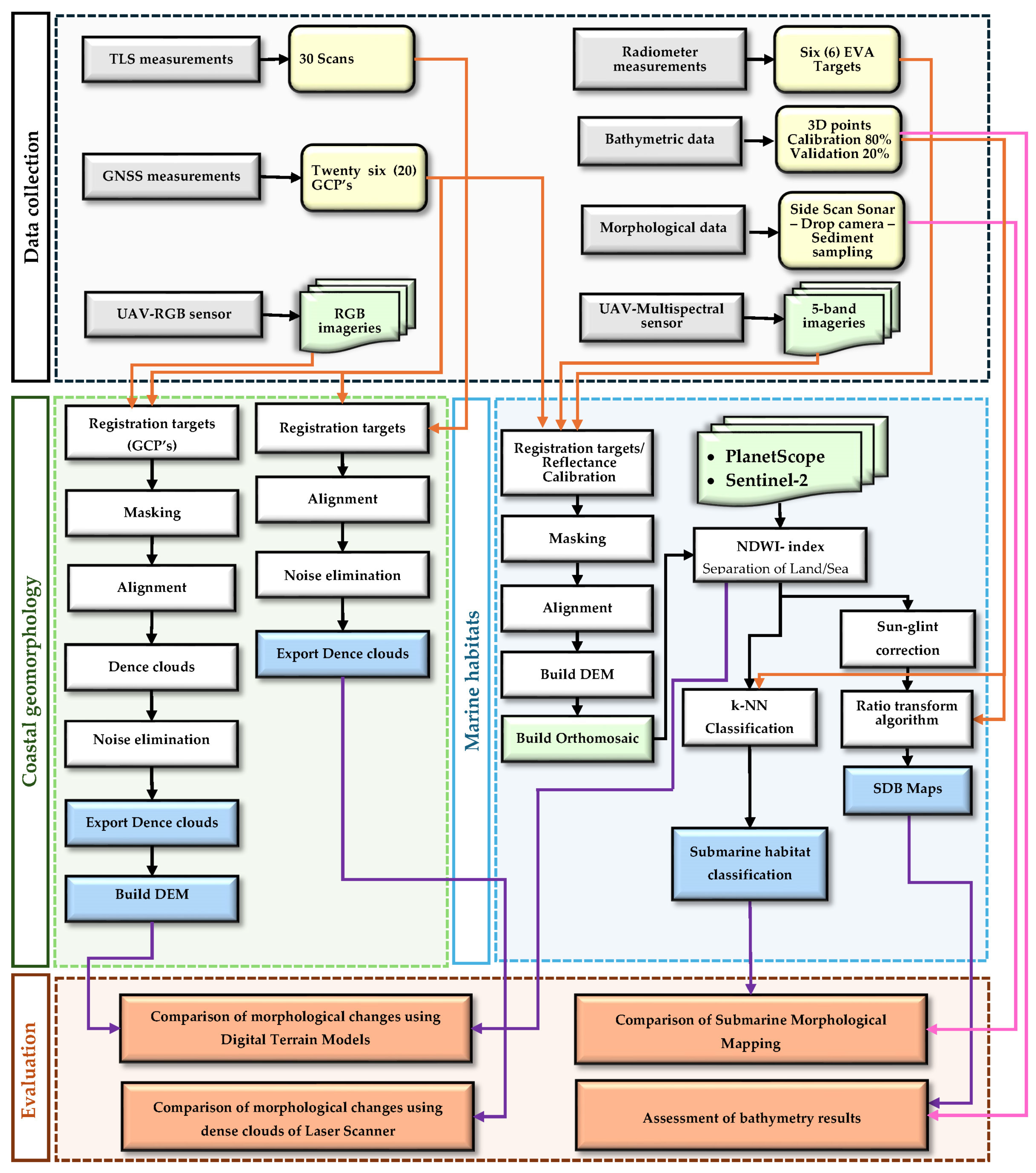
3. Methodology
3.1. Data Collection
3.1.1. In Situ Survey Measurements
3.1.2. Bathymetry and Submarine Morphology
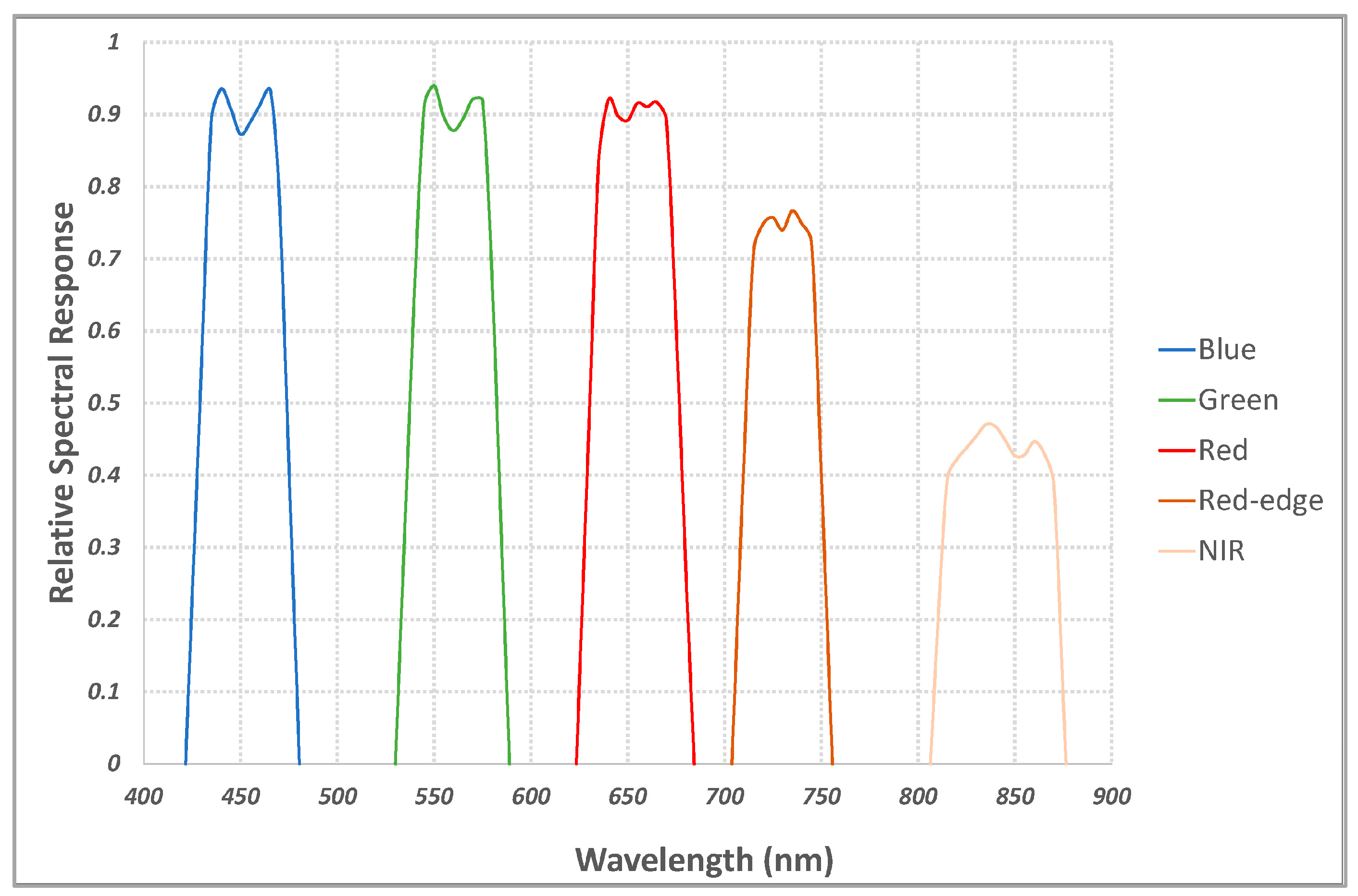
3.1.3. Unmanned Aerial Vehicles (UAV)
3.1.4. Satellite Data
3.2. Processing
3.2.1. Onshore Geomorphology
3.2.2. Bathymetry and Submarine Morphology
4. Results
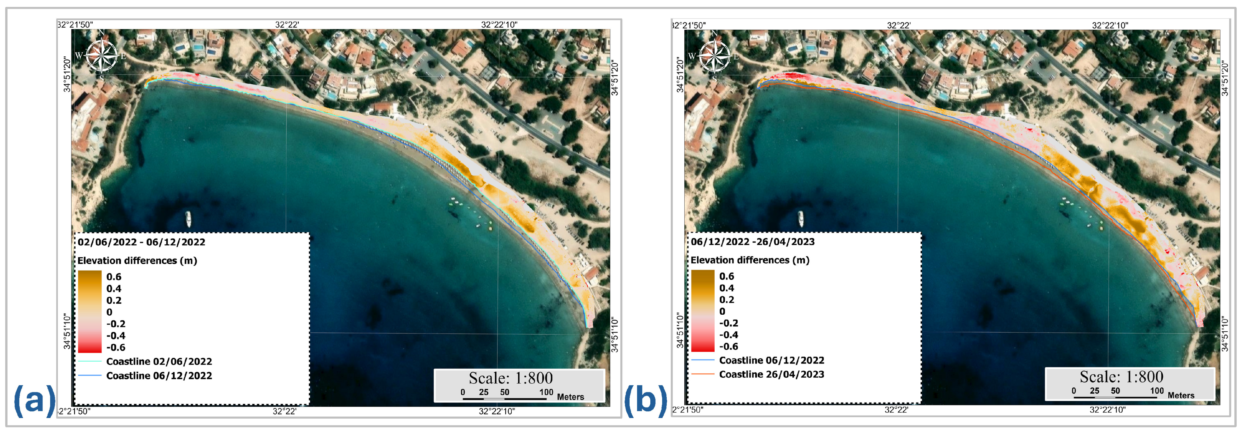
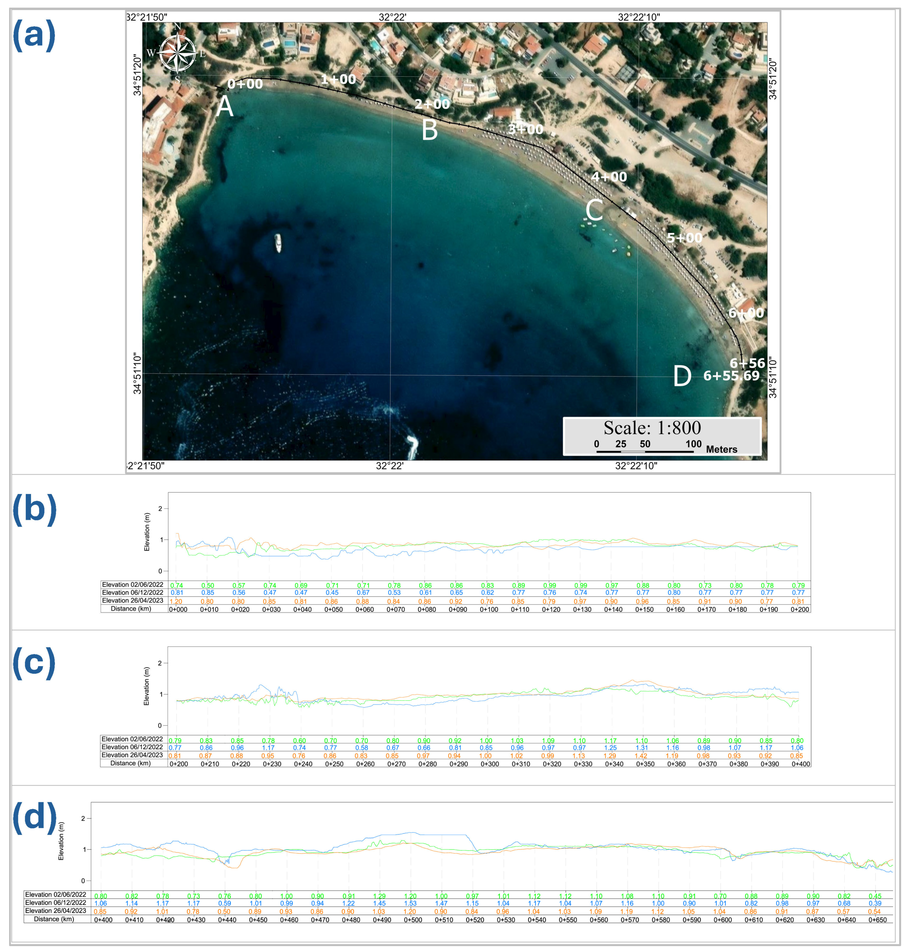
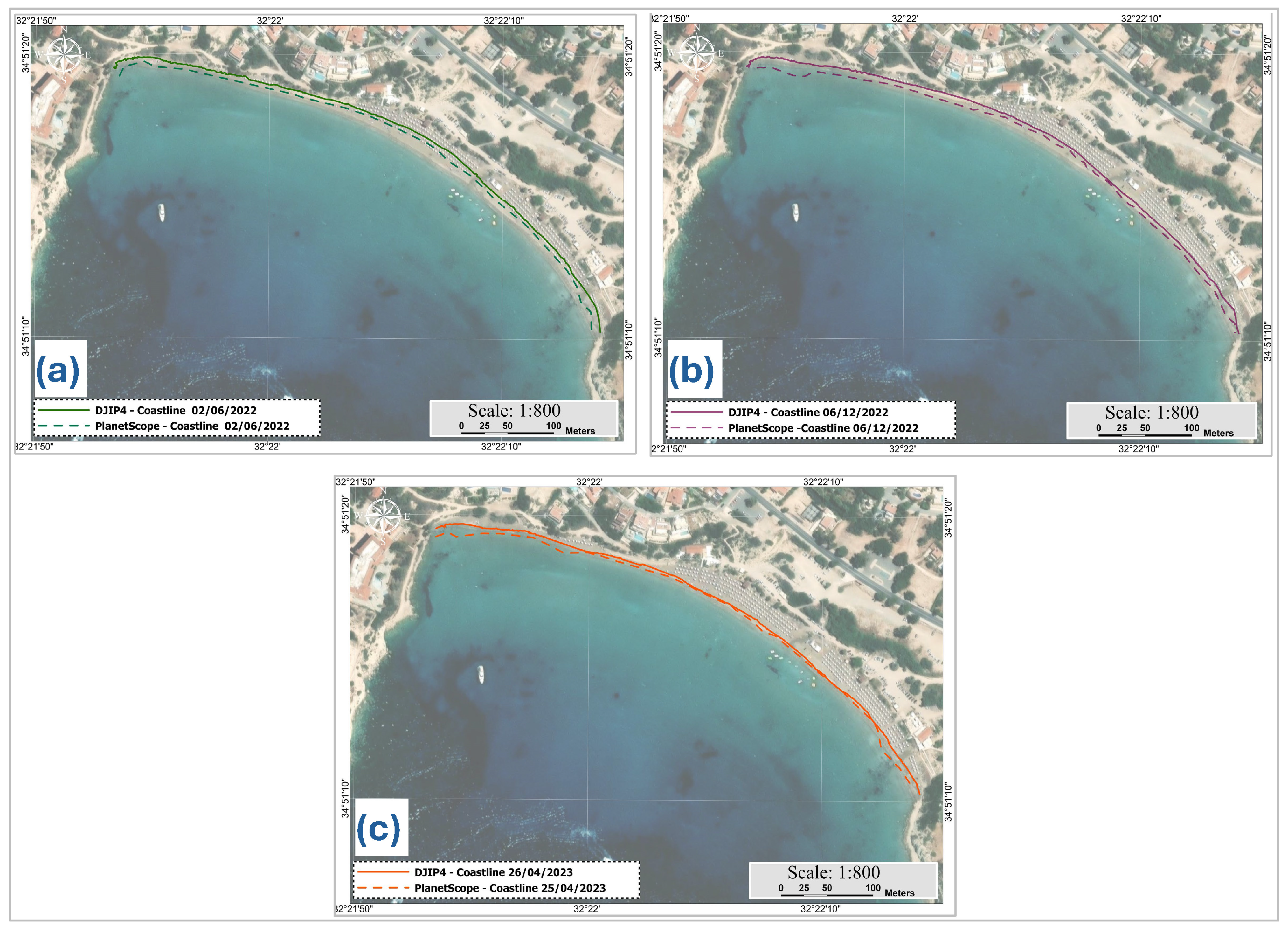
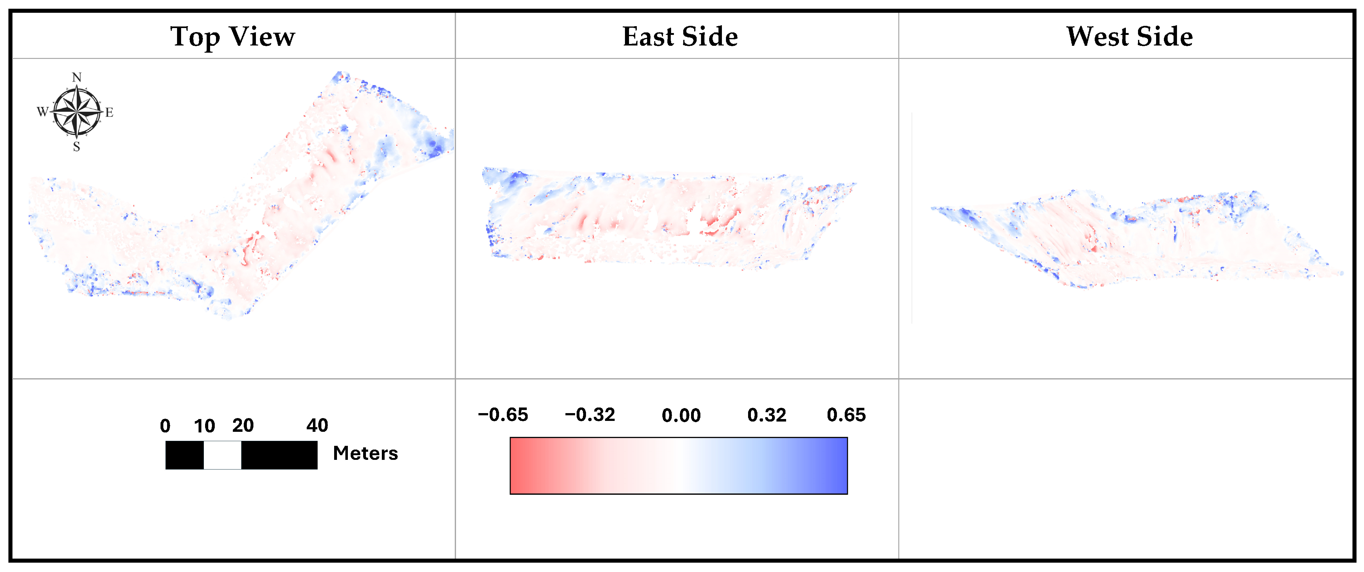
4.1. Onshore Morphology
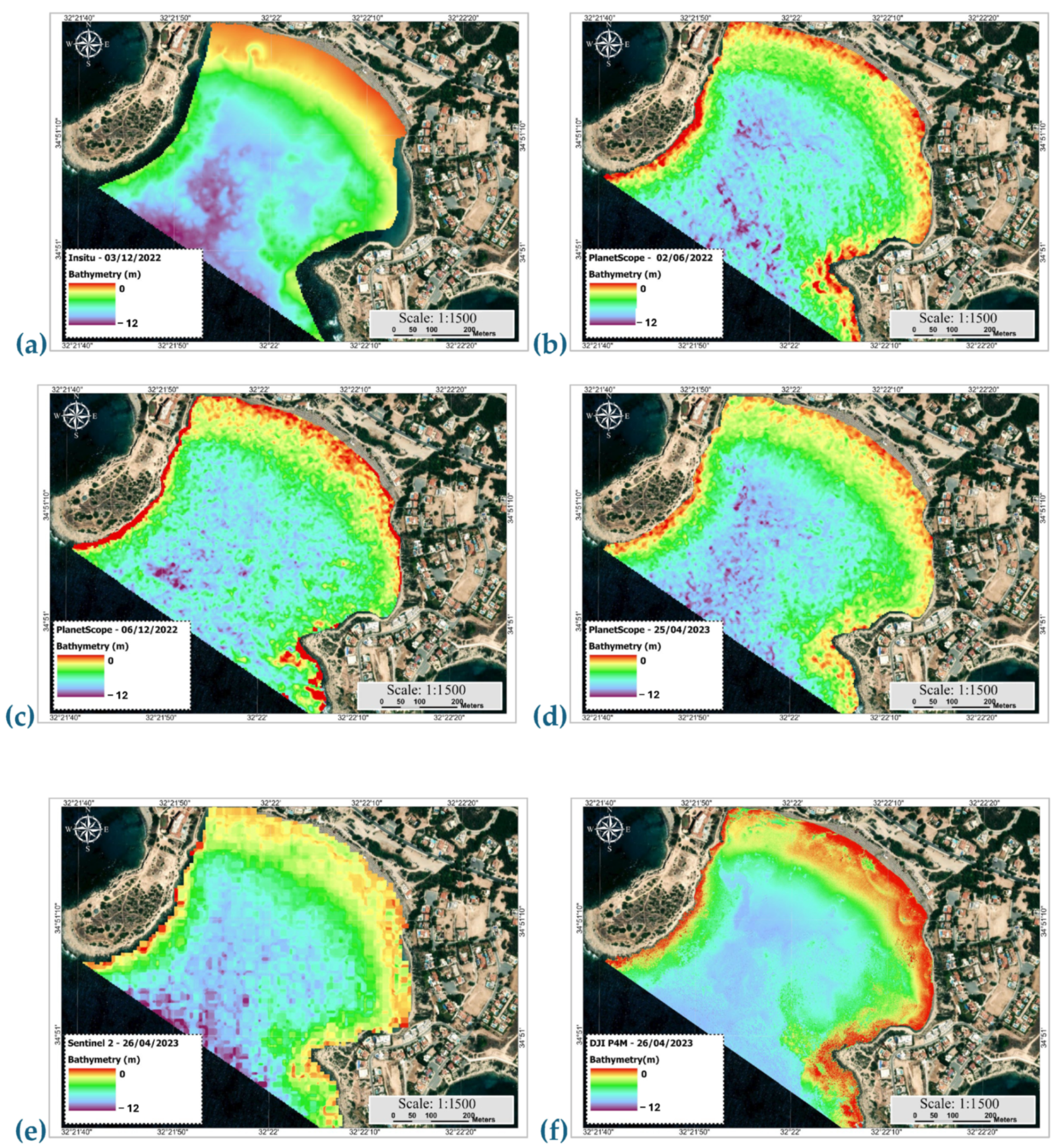
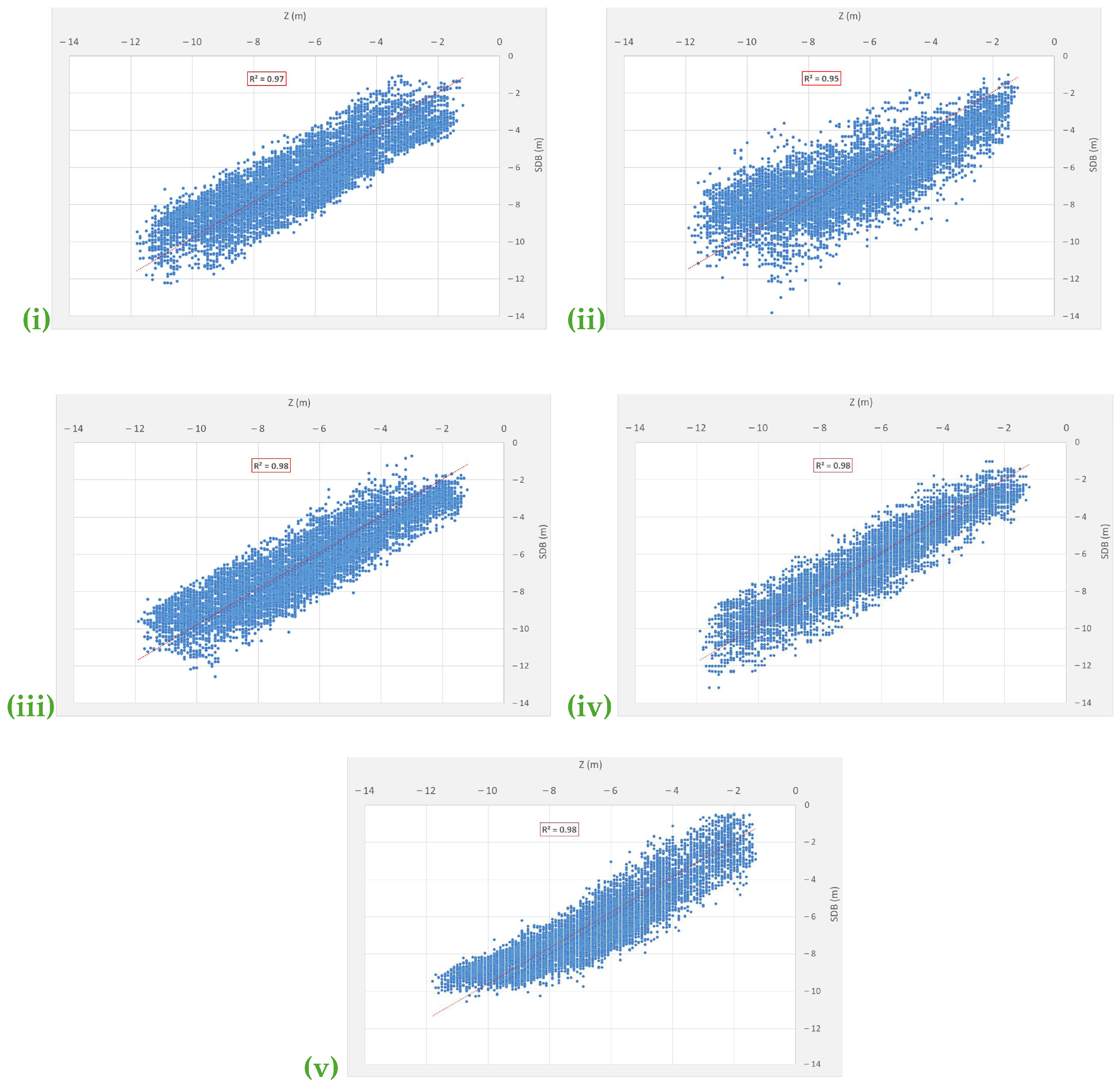
4.2. Bathymetry and Submarine Morphology
5. Discussion
6. Conclusions
Author Contributions
Funding
Data Availability Statement
Acknowledgments
Conflicts of Interest
References
- Field, C.B.; Barros, V.; Stocker, T.F.; Qin, D.; Dokken, D.J.; Ebi, K.J.; Plattner, G.K.; Allen, S.K.; Tignor, M.; Midgley, P.M. Managing the Risks of Extreme Events and Disasters to Advance Climate Change Adaptation: A Special Report of Working Groups I and II of the Intergovernmental Panel on Climate Chang; Cambridge University Press: Cambridge, UK; New York, NY, USA, 2012; 582p. [Google Scholar] [CrossRef]
- Roy, P.; Pal, S.C.; Chakrabortty, R.; Chowdhuri, I.; Saha, A.; Shit, M. Effects of Climate Change and Sea-Level Rise on Coastal Habitat: Vulnerability Assessment, Adaptation Strategies and Policy Recommendations. J. Environ. Manag. 2023, 330, 117187. [Google Scholar] [CrossRef] [PubMed]
- Neumann, B.; Vafeidis, A.T.; Zimmermann, J.; Nicholls, R.J. Future Coastal Population Growth and Exposure to Sea-Level Rise and Coastal Flooding—A Global Assessment. PLoS ONE 2015, 10, e0118571. [Google Scholar] [CrossRef] [PubMed]
- Ackerman, R. The Nest Environment and the Embryonic Development of Sea Turtles; Lutz, P.L., Musick, J.A., Eds.; CRC Press: Boca Raton, FL, USA, 2017; Volume 1, ISBN 9780203737088. [Google Scholar]
- Orlando, L.; Ortega, L.; Defeo, O. Perspectives for Sandy Beach Management in the Anthropocene: Satellite Information, Tourism Seasonality, and Expert Recommendations. Estuar. Coast. Shelf Sci. 2021, 262, 107597. [Google Scholar] [CrossRef]
- Bozzeda, F.; Ortega, L.; Costa, L.L.; Fanini, L.; Barboza, C.A.M.; McLachlan, A.; Defeo, O. Global Patterns in Sandy Beach Erosion: Unraveling the Roles of Anthropogenic, Climatic and Morphodynamic Factors. Front. Mar. Sci. 2023, 10, 1270490. [Google Scholar] [CrossRef]
- Landry, C.E.; Turner, D.; Allen, T. Hedonic Property Prices and Coastal Beach Width. Appl. Econ. Perspect. Policy 2022, 44, 1373–1392. [Google Scholar] [CrossRef]
- UNWTO International Tourism Highlights, 2024 ed.; World Tourism Organization: Madrid, Spain, 2024; ISBN 978-92-844-2579-2.
- Guisado-Pintado, E.; Jackson, D.W.T. Coastal Impact From High-Energy Events and the Importance of Concurrent Forcing Parameters: The Cases of Storm Ophelia (2017) and Storm Hector (2018) in NW Ireland. Front. Earth Sci. 2019, 7, 454617. [Google Scholar] [CrossRef]
- Vousdoukas, M.I.; Ranasinghe, R.; Mentaschi, L.; Plomaritis, T.A.; Athanasiou, P.; Luijendijk, A.; Feyen, L. Sandy Coastlines under Threat of Erosion. Nat. Clim. Change 2020, 10, 260–263. [Google Scholar] [CrossRef]
- Almar, R.; Ranasinghe, R.; Bergsma, E.W.J.; Diaz, H.; Melet, A.; Papa, F.; Vousdoukas, M.; Athanasiou, P.; Dada, O.; Almeida, L.P.; et al. A Global Analysis of Extreme Coastal Water Levels with Implications for Potential Coastal Overtopping. Nat. Commun. 2021, 12, 3775. [Google Scholar] [CrossRef] [PubMed]
- Monioudi, I.N.; Velegrakis, A.F. Beach Carrying Capacity at Touristic 3S Destinations: Its Significance, Projected Decreases and Adaptation Options under Climate Change. J. Tour. Hosp. 2022, 11, 500. [Google Scholar] [CrossRef]
- Komar, P.D. Beach Processes and Sedimentation, 2nd ed.; Prentice Hall: Englewood Cliffs, NJ, USA, 1998; ISBN 0137549385, 9780137549382. [Google Scholar]
- Siemens, T.; Bastola, S. Depth of Closure, a Review of Empirical Formulae and Assessment of Climate Change along the Coast of Louisiana. J. Coast. Conserv. 2024, 28, 71. [Google Scholar] [CrossRef]
- Tsuguo, S. Sunamura Tsuguo Processes of Sea Cliff and Platform Erosion. In CRC Handbook of Coastal Processes and Erosion; CRC Press: Boca Raton, FL, USA, 2018; pp. 233–266. ISBN 9781351072908. [Google Scholar]
- Earlie, C.; Masselink, G.; Russell, P. The Role of Beach Morphology on Coastal Cliff Erosion under Extreme Waves. Earth Surf. Process. Landf. 2018, 43, 1213–1228. [Google Scholar] [CrossRef]
- Serrano, E.; de Sanjosé, J.J.; Gómez-Lende, M.; Sánchez-Fernández, M.; Gómez-Gutiérrez, A. Coastal Retreat and Sea-Cliff Dynamic on the North Atlantic Coast (Gerra Beach, Cantabrian Coast, Spain). Environ. Earth Sci. 2024, 83, 89. [Google Scholar] [CrossRef]
- Allenbach, K.; Garonna, I.; Herold, C.; Monioudi, I.; Giuliani, G.; Lehmann, A.; Velegrakis, A.F. Black Sea Beaches Vulnerability to Sea Level Rise. Environ. Sci. Policy 2015, 46, 95–109. [Google Scholar] [CrossRef]
- Monioudi, I.N.; Velegrakis, A.F.; Chatzistratis, D.; Vousdoukas, M.I.; Savva, C.; Wang, D.; Bove, G.; Mentaschi, L.; Paprotny, D.; Morales-Nápoles, O.; et al. Climate Change—Induced Hazards on Touristic Island Beaches: Cyprus, Eastern Mediterranean. Front. Mar. Sci. 2023, 10, 1188896. [Google Scholar] [CrossRef]
- Monioudi, I.N.; Velegrakis, A.F.; Chatzipavlis, A.E.; Rigos, A.; Karambas, T.; Vousdoukas, M.I.; Hasiotis, T.; Koukourouvli, N.; Peduzzi, P.; Manoutsoglou, E.; et al. Assessment of Island Beach Erosion Due to Sea Level Rise: The Case of the Aegean Archipelago (Eastern Mediterranean). Nat. Hazards Earth Syst. Sci. 2017, 17, 449–466. [Google Scholar] [CrossRef]
- Misiuk, B.; Brown, C.J. Benthic Habitat Mapping: A Review of Three Decades of Mapping Biological Patterns on the Seafloor. Estuar. Coast. Shelf Sci. 2024, 296, 108599. [Google Scholar] [CrossRef]
- Manes, S.; Gama-Maia, D.; Vaz, S.; Pires, A.P.; Tardin, R.H.; Maricato, G.; Bezerra, D.d.S.; Vale, M.M. Nature as a Solution for Shoreline Protection against Coastal Risks Associated with Ongoing Sea-Level Rise. Ocean Coast. Manag. 2023, 235, 106487. [Google Scholar] [CrossRef]
- Nourdi, N.F.; Raphael, O.; Achab, M.; Loudi, Y.; Rudant, J.P.; Minette, T.E.; Kambia, P.; Claude, N.J.; Romaric, N. Integrated Assessment of Coastal Vulnerability in the Bonny Bay: A Combination of Traditional Methods (Simple and AHP) and Machine Learning Approach. Estuaries Coasts 2024, 47, 2670–2695. [Google Scholar] [CrossRef]
- Andreadis, O.; Chatzipavlis, A.; Hasiotis, T.; Monioudi, I.; Manoutsoglou, E.; Velegrakis, A. Assessment of and Adaptation to Beach Erosion in Islands: An Integrated Approach. J. Mar. Sci. Eng. 2021, 9, 859. [Google Scholar] [CrossRef]
- Deng, J.; Yu, H. Modelling Coastal Morphodynamic Evolution under Human Impacts: A Review. J. Mar. Sci. Eng. 2023, 11, 1426. [Google Scholar] [CrossRef]
- Karambas, T.V.; Samaras, A.G. An Integrated Numerical Model for the Design of Coastal Protection Structures. J. Mar. Sci. Eng. 2017, 5, 50. [Google Scholar] [CrossRef]
- Gallerano, F.; Cannata, G.; Lasaponara, F. A New Numerical Model for Simulations of Wave Transformation, Breaking and Long-Shore Currents in Complex Coastal Regions. Int. J. Numer. Methods Fluids 2016, 80, 571–613. [Google Scholar] [CrossRef]
- Ranasinghe, R. Assessing Climate Change Impacts on Open Sandy Coasts: A Review. Earth-Sci. Rev. 2016, 160, 320–332. [Google Scholar] [CrossRef]
- Peduzzi, P.; Velegrakis, A.; Chatenoux, B.; Estrella, M.; Karambas, T. Assessment of the Role of Nearshore Marine Ecosystems to Mitigate Beach Erosion: The Case of Negril (Jamaica). Environments 2022, 9, 62. [Google Scholar] [CrossRef]
- Velegrakis, A.F.; Trygonis, V.; Chatzipavlis, A.E.; Karambas, T.; Vousdoukas, M.I.; Ghionis, G.; Monioudi, I.N.; Hasiotis, T.; Andreadis, O.; Psarros, F. Shoreline Variability of an Urban Beach Fronted by a Beachrock Reef from Video Imagery. Nat. Hazards 2016, 83, 201–222. [Google Scholar] [CrossRef]
- Velegrakis, A.F.; Chatzistratis, D.; Chalazas, T.; Armaroli, C.; Schiavon, E.; Alves, B.; Grigoriadis, D.; Hasiotis, T.; Ieronymidi, E. Earth Observation Technologies, Policies and Legislation for the Coastal Flood Risk Assessment and Management: A European Perspective. Anthr. Coasts 2024, 7, 3. [Google Scholar] [CrossRef]
- Pardo-Pascual, J.E.; Almonacid-Caballer, J.; Cabezas-Rabadán, C.; Fernández-Sarría, A.; Armaroli, C.; Ciavola, P.; Montes, J.; Souto-Ceccon, P.E.; Palomar-Vázquez, J. Assessment of Satellite-Derived Shorelines Automatically Extracted from Sentinel-2 Imagery Using SAET. Coast. Eng. 2024, 188, 104426. [Google Scholar] [CrossRef]
- Palomar-Vázquez, J.; Pardo-Pascual, J.E.; Almonacid-Caballer, J.; Cabezas-Rabadán, C. Shoreline Analysis and Extraction Tool (SAET): A New Tool for the Automatic Extraction of Satellite-Derived Shorelines with Subpixel Accuracy. Remote Sens. 2023, 15, 3198. [Google Scholar] [CrossRef]
- Capperucci, R.M.; Kubicki, A.; Holler, P.; Bartholomä, A. Sidescan Sonar Meets Airborne and Satellite Remote Sensing: Challenges of a Multi-Device Seafloor Classification in Extreme Shallow Water Intertidal Environments. Geo-Mar. Lett. 2020, 40, 117–133. [Google Scholar] [CrossRef]
- He, J.; Zhang, S.; Cui, X.; Feng, W. Remote Sensing for Shallow Bathymetry: A Systematic Review. Earth-Sci. Rev. 2024, 258, 104957. [Google Scholar] [CrossRef]
- Viaña-Borja, S.P.; González-Villanueva, R.; Alejo, I.; Stumpf, R.P.; Navarro, G.; Caballero, I. Satellite-Derived Bathymetry Using Sentinel-2 in Mesotidal Coasts. Coast. Eng. 2025, 195, 104644. [Google Scholar] [CrossRef]
- Evagorou, E.; Argyriou, A.; Papadopoulos, N.; Mettas, C.; Alexandrakis, G.; Hadjimitsis, D. Evaluation of Satellite-Derived Bathymetry from High and Medium-Resolution Sensors Using Empirical Methods. Remote Sens. 2022, 14, 772. [Google Scholar] [CrossRef]
- Hasiotis, T.; Andreadis, O.; Chatzipavlis, A.; Mettas, C.; Evagorou, E.; Kountouri, J.; Hadjimitsis, D.; Christofi, D.; Loizidou, M.; Chrysostomou, G. A Holistic High-Resolution Monitoring Approach in Studying Coastal Erosion of a Highly Touristic Beach, Coral Bay, Cyprus. In Proceedings of the Ninth International Conference on Remote Sensing and Geoinformation of the Environment (RSCy2023), Ayia Napa, Cyprus, 3–5 April 2023; Volume 12786, pp. 376–385. [Google Scholar] [CrossRef]
- Valdazo, J.; Ferrer, N.; Vega, C.; Martín, J.; Luque, Á.; Bergasa, O. Mapping Marine Habitats in a Shallow Beach-Reef Environment Combining Direct Methods and Hyperspectral Remote Sensing. Ocean Coast. Manag. 2024, 255, 107231. [Google Scholar] [CrossRef]
- Specht, M. Methodology for Performing Bathymetric and Photogrammetric Measurements Using UAV and USV Vehicles in the Coastal Zone. Remote Sens. 2024, 16, 3328. [Google Scholar] [CrossRef]
- Tiškus, E.; Vaičiūtė, D.; Bučas, M.; Gintauskas, J. Evaluation of Common Reed (Phragmites australis) Bed Changes in the Context of Management Using Earth Observation and Automatic Threshold. Eur. J. Remote Sens. 2023, 56, 100–114. [Google Scholar] [CrossRef]
- Bio, A.; Gonçalves, J.A.; Magalhães, A.; Pinheiro, J.; Bastos, L. Combining Low-Cost Sonar and High-Precision Global Navigation Satellite System for Shallow Water Bathymetry. Estuaries Coasts 2022, 45, 1000–1011. [Google Scholar] [CrossRef]
- Guillén, J.; Simarro, G.; Calvete, D.; Ribas, F.; Fernández-Mora, A.; Orfila, A.; Falqués, A.; de Swart, R.; Sancho-García, A.; Durán, R. Sediment Leakage on the Beach and Upper Shoreface Due to Extreme Storms. Mar. Geol. 2024, 468, 107207. [Google Scholar] [CrossRef]
- Panagou, T.; Hasiotis, T.; Velegrakis, A.; Karambas, T.; Oikonomou, E.; Dimitriadis, C. Erosion Status of a Sea Cliff Promontory Bounding an Ecologically Important Beach. J. Coast. Conserv. 2020, 24, 1–17. [Google Scholar] [CrossRef]
- Andriolo, U.; Almeida, L.P.; Almar, R. Coupling Terrestrial LiDAR and Video Imagery to Perform 3D Intertidal Beach Topography. Coast. Eng. 2018, 140, 232–239. [Google Scholar] [CrossRef]
- Brodie, K.L.; Slocum, R.K.; McNinch, J.E. New Insights into the Physical Drivers of Wave Runup from a Continuously Operating Terrestrial Laser Scanner. In Proceedings of the Ocean, 2012 MTS/IEEE Harnessing Power Ocean, Hampton Roads, VA, USA, 14–19 October 2012. [Google Scholar] [CrossRef]
- Harry, M.; Zhang, H.; Lemckert, C.; Colleter, G.; Blenkinsopp, C. Observation of Surf Zone Wave Transformation Using LiDAR. Appl. Ocean Res. 2018, 78, 88–98. [Google Scholar] [CrossRef]
- Klopfer, F.; Hämmerle, M.; Höfle, B. Assessing the Potential of a Low-Cost 3-D Sensor in Shallow-Water Bathymetry. IEEE Geosci. Remote Sens. Lett. 2017, 14, 1388–1392. [Google Scholar] [CrossRef]
- Panagou, T.; Oikonomou, E.; Hasiotis, T.; Velegrakis, A.F. Shallow Water Bathymetry Derived from Green Wavelength Terrestrial Laser Scanner. Mar. Geod. 2020, 43, 472–492. [Google Scholar] [CrossRef]
- Letortu, P.; Costa, S.; Maquaire, O.; Delacourt, C.; Augereau, E.; Davidson, R.; Suanez, S.; Nabucet, J. Retreat Rates, Modalities and Agents Responsible for Erosion along the Coastal Chalk Cliffs of Upper Normandy: The Contribution of Terrestrial Laser Scanning. Geomorphology 2015, 245, 3–14. [Google Scholar] [CrossRef]
- Poursanidis, D.; Topouzelis, K.; Chrysoulakis, N. Mapping Coastal Marine Habitats and Delineating the Deep Limits of the Neptune’s Seagrass Meadows Using Very High Resolution Earth Observation Data. Int. J. Remote Sens. 2018, 39, 8670–8687. [Google Scholar] [CrossRef]
- Traganos, D.; Aggarwal, B.; Poursanidis, D.; Topouzelis, K.; Chrysoulakis, N.; Reinartz, P. Towards Global-Scale Seagrass Mapping and Monitoring Using Sentinel-2 on Google Earth Engine: The Case Study of the Aegean and Ionian Seas. Remote Sens. 2018, 10, 1227. [Google Scholar] [CrossRef]
- Rende, S.F.; Bosman, A.; Di Mento, R.; Bruno, F.; Lagudi, A.; Irving, A.D.; Dattola, L.; Di Giambattista, L.; Lanera, P.; Proietti, R.; et al. Ultra-High-Resolution Mapping of Posidonia oceanica (L.) Delile Meadows through Acoustic, Optical Data and Object-Based Image Classification. J. Mar. Sci. Eng. 2020, 8, 647. [Google Scholar] [CrossRef]
- Doukari, M.; Katsanevakis, S.; Soulakellis, N.; Topouzelis, K. The Effect of Environmental Conditions on the Quality of UAS Orthophoto-Maps in the Coastal Environment. ISPRS Int. J. Geo-Inform. 2021, 10, 18. [Google Scholar] [CrossRef]
- Tzafaridi, V.M.; Petsimeris, I.; Hasiotis, T. Evaluation of Habitat Distribution and Human Imprints around an Insular Open-Pit, Gyali Island, Southeast Aegean Sea. In Proceedings of the Tenth International Conference on Remote Sensing and Geoinformation of the Environment (RSCy2024), Paphos, Cyprus, 8–9 April 2024; Volume 13212, pp. 87–95. [Google Scholar] [CrossRef]
- Borrelli, M.; Smith, T.L.; Mague, S.T. Vessel-Based, Shallow Water Mapping with a Phase-Measuring Sidescan Sonar. Estuaries Coasts 2022, 45, 961–979. [Google Scholar] [CrossRef]
- Dimas, X.; Fakiris, E.; Christodoulou, D.; Georgiou, N.; Geraga, M.; Papathanasiou, V.; Orfanidis, S.; Kotomatas, S.; Papatheodorou, G. Marine Priority Habitat Mapping in a Mediterranean Conservation Area (Gyaros, South Aegean) through Multi-Platform Marine Remote Sensing Techniques. Front. Mar. Sci. 2022, 9, 953462. [Google Scholar] [CrossRef]
- Kassouk, Z.; Ayari, E.; Deffontaines, B.; Ouaja, M. Monitoring Coastal Evolution and Geomorphological Processes Using Time-Series Remote Sensing and Geospatial Analysis: Application Between Cape Serrat and Kef Abbed, Northern Tunisia. Remote Sens. 2024, 16, 3895. [Google Scholar] [CrossRef]
- Chatzıpavlıs, A.; Andreadıs, O.; Psarros, F.; Hasıotıs, T.; Velegrakıs, A.; Evagorou, E.; Loızıdı, M.; Chrysostomou, G. Morphological Changes Recorded from an Automated Beach Optical Monitoring System in a Highly Touristic Pocket Beach, Coral Bay, Pegeia, Cyprus. In Proceedings of the 18th International Conference on Environmental Science and Technology, Athens, Greece, 30 August–2 September 2023; pp. 1–4. [Google Scholar]
- Jessin, J.; Heinzlef, C.; Long, N.; Serre, D. A Systematic Review of UAVs for Island Coastal Environment and Risk Monitoring: Towards a Resilience Assessment. Drones 2023, 7, 206. [Google Scholar] [CrossRef]
- Kovanič, Ľ.; Topitzer, B.; Peťovský, P.; Blišťan, P.; Gergeľová, M.B.; Blišťanová, M. Review of Photogrammetric and Lidar Applications of UAV. Appl. Sci. 2023, 13, 6732. [Google Scholar] [CrossRef]
- Labshere Reflectance Materials and Coatings—Technical Guide; Labsphere, Inc.: North Sutton, NH, USA, 2011.
- Rees, W.G. Physical Principles of Remote Sensing, 3rd ed.; Cambridge University Press: New York, NY, USA, 2013; ISBN 978-1-107-00473-3. [Google Scholar]
- NASA Landsat Science: A Lambertian Reflector. Available online: https://landsat.gsfc.nasa.gov/about/lambertian-reflector (accessed on 13 April 2025).
- Ponce-Alcántara, S.; Arangú, A.V.; Plaza, G.S. The Importance of Optical Characterization of PV Backsheets in Improving Solar Module Power. In Proceedings of the 8th International Photovoltaic Power Generation Conference Exhibition, Shanghai, China, 11–13 June 2015. [Google Scholar]
- Padró, O.-C.; Muñoz, F.-J.; Ávila, L.Á.; Pesquer, L.; Pons, X. Radiometric Correction of Landsat-8 and Sentinel-2A Scenes Using Drone Imagery in Synergy with Field Spectroradiometry. J. Remote Sens. 2018, 10, 1687. [Google Scholar] [CrossRef]
- Padró, J.; Carabassa, V.; Balagué, J.; Brotons, L.; Alcañiz, J.M.; Pons, X. Monitoring Opencast Mine Restorations Using Unmanned Aerial System (UAS) Imagery. Sci. Total Environ. 2019, 657, 1602–1614. [Google Scholar] [CrossRef]
- Jeong, Y.; Yu, J.; Wang, L.; Shin, H.; Koh, S.M.; Park, G. Cost-Effective Reflectance Calibration Method for Small UAV Images. Int. J. Remote Sens. 2018, 39, 7225–7250. [Google Scholar] [CrossRef]
- Jiang, S.; Jiang, C.; Jiang, W. Efficient Structure from Motion for Large-Scale UAV Images: A Review and a Comparison of SfM Tools. ISPRS J. Photogramm. Remote Sens. 2020, 167, 230–251. [Google Scholar] [CrossRef]
- Alexiou, S.; Deligiannakis, G.; Pallikarakis, A.; Papanikolaou, I.; Psomiadis, E.; Reicherter, K. Comparing High Accuracy T-LiDAR and UAV-SfM Derived Point Clouds for Geomorphological Change Detection. ISPRS Int. J. Geo-Inform. 2021, 10, 367. [Google Scholar] [CrossRef]
- Storch, M.; Kisliuk, B.; Jarmer, T.; Waske, B.; de Lange, N. Comparative Analysis of UAV-Based LiDAR and Photogrammetric Systems for the Detection of Terrain Anomalies in a Historical Conflict Landscape. Sci. Remote Sens. 2025, 11, 100191. [Google Scholar] [CrossRef]
- Agisoft LLC Agisoft Metashape 2024. Available online: https://www.agisoft.com (accessed on 13 April 2025).
- Esri ArcGIS Pro 2024. Available online: https://www.esri.com/en-us/arcgis/products/arcgis-pro/overview (accessed on 13 April 2025).
- Amodio, A.M.; Di Paola, G.; Rosskopf, C.M. Monitoring Coastal Vulnerability by Using DEMs Based on UAV Spatial Data. ISPRS Int. J. Geo-Inform. 2022, 11, 155. [Google Scholar] [CrossRef]
- Pagán, J.I.; Bañón, L.; López, I.; Bañón, C.; Aragonés, L. Monitoring the Dune-Beach System of Guardamar Del Segura (Spain) Using UAV, SfM and GIS Techniques. Sci. Total Environ. 2019, 687, 1034–1045. [Google Scholar] [CrossRef]
- Chapapría, V.E.; Peris, J.S.; González-Escrivá, J.A. Coastal Monitoring Using Unmanned Aerial Vehicles (UAVs) for the Management of the Spanish Mediterranean Coast: The Case of Almenara-Sagunto. Int. J. Environ. Res. Public Health 2022, 19, 5457. [Google Scholar] [CrossRef] [PubMed]
- Leica Geosystems AG Leica Cyclone 2024. Available online: https://leica-geosystems.com/products/laser-scanners/software/leica-cyclone/leica-cyclone-register-360 (accessed on 13 April 2025).
- CloudCompare CloudCompare (Version 2.12.4) [GPL Software] 2022. Available online: https://www.cloudcompare.org (accessed on 13 April 2025).
- Lague, D.; Brodu, N.; Leroux, J. Accurate 3D Comparison of Complex Topography with Terrestrial Laser Scanner: Application to the Rangitikei Canyon (N-Z). ISPRS J. Photogramm. Remote Sens. 2013, 82, 10–26. [Google Scholar] [CrossRef]
- Autodesk AutoCAD Civil 3D 2018. Available online: https://www.autodesk.com/products/autocad-civil-3d/overview (accessed on 13 April 2025).
- Folk, R.L. Petrologie of Sedimentary Rocks; Hemphill’s: Austin, TX, USA, 1980; ISBN 0-914696-14-9. [Google Scholar]
- Blott, S.J.; Pye, K. GRADISTAT: A Grain Size Distribution and Statistics Package for the Analysis of Unconsolidated Sediments. Earth Surf. Process. Landf. 2001, 26, 1237–1248. [Google Scholar] [CrossRef]
- McFeeters, S.K. The Use of the Normalized Difference Water Index (NDWI) in the Delineation of Open Water Features. Int. J. Remote Sens. 1996, 17, 1425–1432. [Google Scholar] [CrossRef]
- Stumpf, R.P.; Holderied, K.; Sinclair, M. Determination of Water Depth with High-Resolution Satellite Imagery over Variable Bottom Types. Limnol. Oceanogr. 2003, 48, 547–556. [Google Scholar] [CrossRef]
- Kayhan, E.C.; Ekmekcioğlu, Ö. Coupling Different Machine Learning and Meta-Heuristic Optimization Techniques to Generate the Snow Avalanche Susceptibility Map in the French Alps. Water 2024, 16, 3247. [Google Scholar] [CrossRef]
- Sun, S.; Huang, R. An Adaptive K-Nearest Neighbor Algorithm. In Proceedings of the 2010 Seventh International Conference on Fuzzy Systems and Knowledge Discovery, Yantai, China, 10–12 August 2010; Volume 1, pp. 91–94. [Google Scholar] [CrossRef]
- Fix, E.; Hodges, J.L. Discriminatory Analysis. Nonparametric Discrimination: Consistency Properties. Int. Stat. Rev./Rev. Int. Stat. 1989, 57, 238. [Google Scholar] [CrossRef]
- Nababan, B.; Mastu, L.O.K.; Idris, N.H.; Panjaitan, J.P. Shallow-Water Benthic Habitat Mapping Using Drone with Object Based Image Analyses. Remote Sens. 2021, 13, 4452. [Google Scholar] [CrossRef]
- Valderrama-Landeros, L.; Flores-de-Santiago, F.; Álvarez-Sánchez, L.F.; Flores-Verdugo, F.; Rodríguez-Sobreyra, R. The Influence of Spatial Resolution on Coastline Detection by Means of Multisource Remote Sensing Data. Remote Sens. Appl. Soc. Environ. 2024, 35, 101258. [Google Scholar] [CrossRef]
- Chen, C.; Chen, H.; Liang, J.; Huang, W.; Xu, W.; Li, B.; Wang, J.; Wu, Q.; Shen, X.; Li, J.; et al. Extraction of Water Body Information from Remote Sensing Imagery While Considering Greenness and Wetness Based on Tasseled Cap Transformation. Remote Sens. 2022, 14, 3001. [Google Scholar] [CrossRef]
- PLANET Planet Imagery Product Specifications. 2023. Available online: https://assets.planet.com/docs/Planet_Combined_Imagery_Product_Specs_letter_screen.pdf (accessed on 13 April 2025).
- Melet, A.; Teatini, P.; Le Cozannet, G.; Jamet, C.; Conversi, A.; Benveniste, J.; Almar, R. Earth Observations for Monitoring Marine Coastal Hazards and Their Drivers. Surv. Geophys. 2020, 41, 1489–1534. [Google Scholar] [CrossRef]
- United Nations Framework Convention on Climate Change; Executive Committee of the Warsaw International Mechanism for loss and Damage. Policy Brief: Technologies for Averting, Minimizing and Addressing Loss and Damage in Coastal Zones; United Nations Framework Convention on Climate Change; Executive Committee of the Warsaw International Mechanism for loss and Damage: Bonn, Germany, 2020; Available online: https://unfccc.int/process-and-meetings/bodies/constituted-bodies/key-knowledge-products-2023/2024/executive-committee-of-the-warsaw-international-mechanism-for-loss-and-damage/policy-brief-technologies-for-averting-minimizing-and-addressing-loss-and-damage-in-coastal (accessed on 13 April 2025).
- Wicaksono, P.; Wulandari, S.A.; Lazuardi, W.; Munir, M. Sentinel-2 Images Deliver Possibilities for Accurate and Consistent Multi-Temporal Benthic Habitat Maps in Optically Shallow Water. Remote Sens. Appl. Soc. Environ. 2021, 23, 100572. [Google Scholar] [CrossRef]
- Chatzipavlis, A.; Tsekouras, G.E.; Trygonis, V.; Velegrakis, A.F.; Tsimikas, J.; Rigos, A.; Hasiotis, T.; Salmas, C. Modeling Beach Realignment Using a Neuro-Fuzzy Network Optimized by a Novel Backtracking Search Algorithm. Neural Comput. Appl. 2018, 31, 1747–1763. [Google Scholar] [CrossRef]
- Casella, E.; Drechsel, J.; Winter, C.; Benninghoff, M.; Rovere, A. Accuracy of Sand Beach Topography Surveying by Drones and Photogrammetry. Geo-Mar. Lett. 2020, 40, 255–268. [Google Scholar] [CrossRef]
- Alessio, P.; Keller, E.A. Short-Term Patterns and Processes of Coastal Cliff Erosion in Santa Barbara, California. Geomorphology 2020, 353, 106994. [Google Scholar] [CrossRef]
- Tyszkowski, S.; Zbucki, Ł.; Kaczmarek, H.; Duszyński, F.; Strzelecki, M.C. Terrestrial Laser Scanning for the Detection of Coastal Changes along Rauk Coasts of Gotland, Baltic Sea. Remote Sens. 2023, 15, 1667. [Google Scholar] [CrossRef]
- Roulland, T.; Maquaire, O.; Costa, S.; Medjkane, M.; Davidson, R.; Fauchard, C.; Antoine, R. Seasonal Activity Quantification of Coast Badlands by TLS Monitoring over Five Years at the “Vaches Noires” Cliffs (Normandy, France). Geomorphology 2022, 400, 108083. [Google Scholar] [CrossRef]
- Ashphaq, M.; Srivastava, P.K.; Mitra, D. Review of Near-Shore Satellite Derived Bathymetry: Classification and Account of Five Decades of Coastal Bathymetry Research. J. Ocean Eng. Sci. 2021, 6, 340–359. [Google Scholar] [CrossRef]
- Casal, G.; Hedley, J.D.; Monteys, X.; Harris, P.; Cahalane, C.; McCarthy, T. Satellite-Derived Bathymetry in Optically Complex Waters Using a Model Inversion Approach and Sentinel-2 Data. Estuar. Coast. Shelf Sci. 2020, 241, 106814. [Google Scholar] [CrossRef]
- Vrdoljak, L.; Kilić Pamuković, J. Assessment of Atmospheric Correction Processors and Spectral Bands for Satellite-Derived Bathymetry Using Sentinel-2 Data in the Middle Adriatic. Hydrology 2022, 9, 215. [Google Scholar] [CrossRef]
- Evagorou, E.; Mettas, C.; Agapiou, A.; Themistocleous, K.; Hadjimitsis, D. Bathymetric Maps from Multi-Temporal Analysis of Sentinel-2 Data: The Case Study of Limassol, Cyprus. Adv. Geosci. 2019, 45, 397–407. [Google Scholar] [CrossRef]
- Li, Z.; Peng, Z.; Zhang, Z.; Chu, Y.; Xu, C.; Yao, S.; García-Fernández, Á.F.; Zhu, X.; Yue, Y.; Levers, A.; et al. Exploring Modern Bathymetry: A Comprehensive Review of Data Acquisition Devices, Model Accuracy, and Interpolation Techniques for Enhanced Underwater Mapping. Front. Mar. Sci. 2023, 10, 1178845. [Google Scholar] [CrossRef]
- Apostolopoulos, D.N.; Nikolakopoulos, K.G. Assessment and Quantification of the Accuracy of Low- and High-Resolution Remote Sensing Data for Shoreline Monitoring. ISPRS Int. J. Geo-Inform. 2020, 9, 391. [Google Scholar] [CrossRef]
- Alevizos, E.; Roussos, A.; Alexakis, D.D. Geomorphometric Analysis of Nearshore Sedimentary Bedforms from High-Resolution Multi-Temporal Satellite-Derived Bathymetry. Geocarto Int. 2022, 37, 8906–8923. [Google Scholar] [CrossRef]
- Wei, C.; Xiao, Y.; Fu, D.; Zhou, T. Impact of Turbidity on Satellite-Derived Bathymetry: Comparative Analysis Across Seven Ports in the South China Sea. Remote Sens. 2024, 16, 4349. [Google Scholar] [CrossRef]
- Papakonstantinou, A.; Stamati, C.; Topouzelis, K. Comparison of True-Color and Multispectral Unmanned Aerial Systems Imagery for Marine Habitat Mapping Using Object-Based Image Analysis. Remote Sens. 2020, 12, 554. [Google Scholar] [CrossRef]
- Ventura, D.; Bruno, M.; Jona Lasinio, G.; Belluscio, A.; Ardizzone, G. A Low-Cost Drone Based Application for Identifying and Mapping of Coastal Fish Nursery Grounds. Estuar. Coast. Shelf Sci. 2016, 171, 85–98. [Google Scholar] [CrossRef]


| A/A | Satellite | Product Name | Resolution (m) | Date Acquisition | Sensing Time | Cloud Coverage % |
|---|---|---|---|---|---|---|
| 1 | PlanetScope | 02062022_Coral_psscene_analytic_8b_sr_udm2 | 3 | 2 June 2022 | 07:38 | 0.00 |
| 2 | PlanetScope | 06122022_Coral_psscene_analytic_8b_sr_udm2 | 3 | 6 December 2022 | 07:38 | 14 |
| 3 | PlanetScope | 20230425_074318_43_24ab_3B_AnalyticMS_SR_8b_clip | 3 | 25 April 2023 | 07:43 | 3.47 |
| 4 | Sentinel 2 | S2A_MSIL2A_20230426T083601_N0509_R064_T36SVD_20230426T130804 | 10 | 26 April 2023 | 08:36 | 40.49 |
| A/A | Dates | X Error (cm) | Y Error (cm) | Z Error (cm) | XY Error (cm) | Total Error (cm) |
|---|---|---|---|---|---|---|
| 1 | 2 June 2022 | 1.63 | 1.60 | 0.65 | 2.28 | 2.37 |
| 2 | 6 December 2022 | 2.23 | 2.98 | 0.95 | 3.72 | 3.84 |
| 3 | 26 April 2023 | 1.58 | 1.52 | 0.80 | 2.19 | 2.33 |
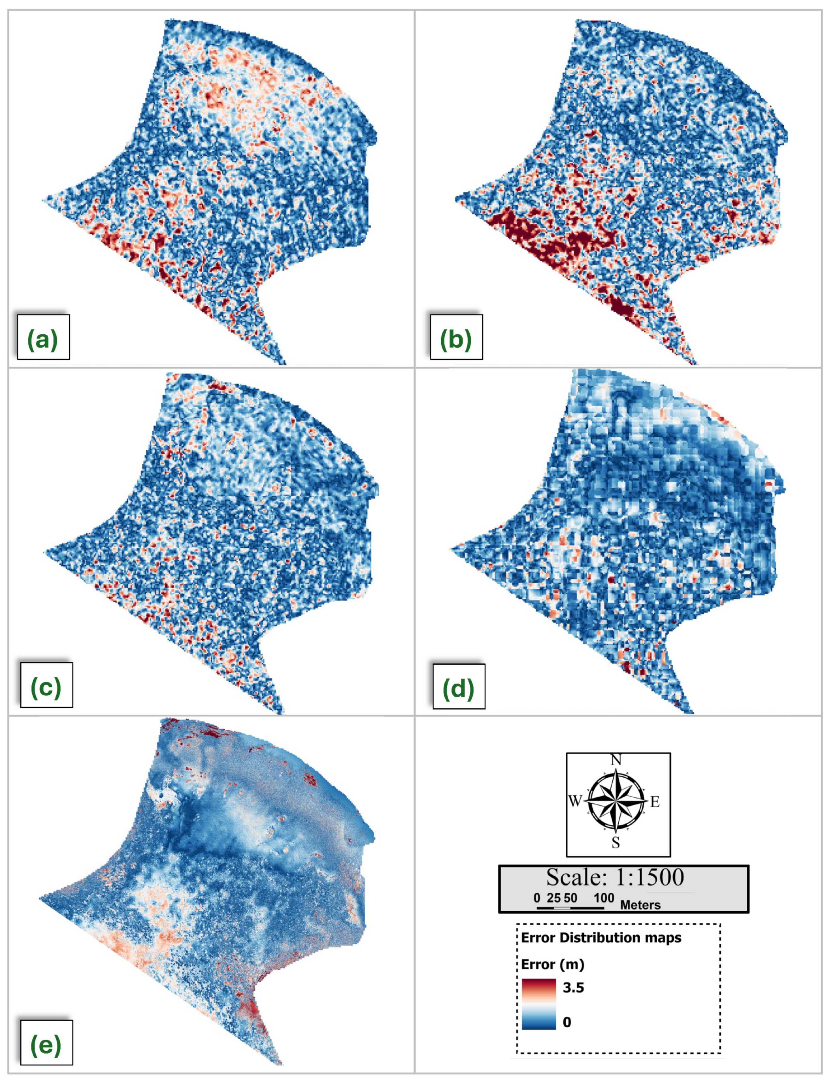
| Satellite | Date Acquisition | R2 | RMSE (m) | |
|---|---|---|---|---|
| (a) | PlanetScope | 2 June 2022 | 0.97 | 1.20 |
| (b) | PlanetScope | 6 December 2022 | 0.95 | 1.52 |
| (c) | PlanetScope | 25 April 2023 | 0.98 | 1.10 |
| (d) | DJIP4M | 26 April 2023 | 0.98 | 1.02 |
| (e) | Sentinel 2 | 26 April 2023 | 0.98 | 0.92 |
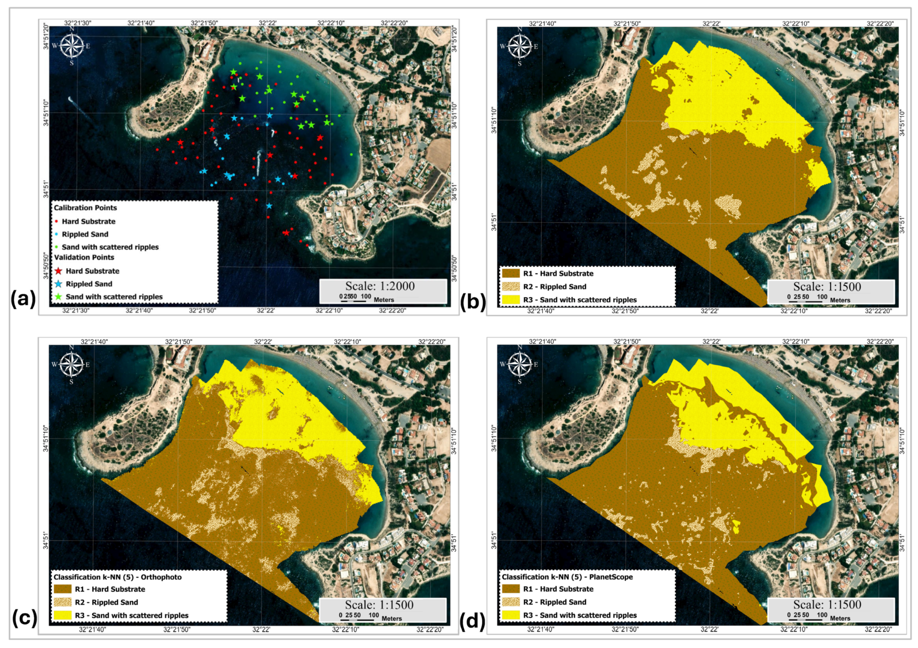
| Ground Truth | |||||
|---|---|---|---|---|---|
| Hard Substrate | Rippled Sand | Sand with Scattered Ripples | Sum | ||
| Training Data | Hard substrate | 596 | 3 | 22 | 621 |
| Rippled sand | 61 | 51 | 12 | 124 | |
| Sand with scattered ripples | 9 | 1 | 245 | 255 | |
| Sum | 666 | 55 | 279 | 1000 | |
| Producers’ accuracy | 0.89 | 0.93 | 0.88 | ||
| Users’ accuracy | 0.96 | 0.41 | 0.96 | ||
| KIA per class | 0.88 | 0.44 | 0.91 | ||
| Total accuracy | 0.89 | ||||
| Overall, Kappa | 0.79 | ||||
| Ground Truth | |||||
|---|---|---|---|---|---|
| Hard Substrate | Rippled Sand | Sand with Scattered Ripples | Sum | ||
| Training Data | Hard substrate | 596 | 37 | 56 | 689 |
| Rippled sand | 49 | 17 | 9 | 75 | |
| Sand with scattered ripples | 21 | 1 | 214 | 236 | |
| Sum | 666 | 55 | 279 | 1000 | |
| Producers’ accuracy | 0.89 | 0.31 | 0.77 | ||
| Users’ accuracy | 0.87 | 0.23 | 0.91 | ||
| KIA per class | 0.94 | 0.73 | 0.84 | ||
| Total accuracy | 0.83 | ||||
| Overall, Kappa | 0.63 | ||||
Disclaimer/Publisher’s Note: The statements, opinions and data contained in all publications are solely those of the individual author(s) and contributor(s) and not of MDPI and/or the editor(s). MDPI and/or the editor(s) disclaim responsibility for any injury to people or property resulting from any ideas, methods, instructions or products referred to in the content. |
© 2025 by the authors. Licensee MDPI, Basel, Switzerland. This article is an open access article distributed under the terms and conditions of the Creative Commons Attribution (CC BY) license (https://creativecommons.org/licenses/by/4.0/).
Share and Cite
Evagorou, E.; Hasiotis, T.; Petsimeris, I.T.; Monioudi, I.N.; Andreadis, O.P.; Chatzipavlis, A.; Christofi, D.; Kountouri, J.; Stylianou, N.; Mettas, C.; et al. A Holistic High-Resolution Remote Sensing Approach for Mapping Coastal Geomorphology and Marine Habitats. Remote Sens. 2025, 17, 1437. https://doi.org/10.3390/rs17081437
Evagorou E, Hasiotis T, Petsimeris IT, Monioudi IN, Andreadis OP, Chatzipavlis A, Christofi D, Kountouri J, Stylianou N, Mettas C, et al. A Holistic High-Resolution Remote Sensing Approach for Mapping Coastal Geomorphology and Marine Habitats. Remote Sensing. 2025; 17(8):1437. https://doi.org/10.3390/rs17081437
Chicago/Turabian StyleEvagorou, Evagoras, Thomas Hasiotis, Ivan Theophilos Petsimeris, Isavela N. Monioudi, Olympos P. Andreadis, Antonis Chatzipavlis, Demetris Christofi, Josephine Kountouri, Neophytos Stylianou, Christodoulos Mettas, and et al. 2025. "A Holistic High-Resolution Remote Sensing Approach for Mapping Coastal Geomorphology and Marine Habitats" Remote Sensing 17, no. 8: 1437. https://doi.org/10.3390/rs17081437
APA StyleEvagorou, E., Hasiotis, T., Petsimeris, I. T., Monioudi, I. N., Andreadis, O. P., Chatzipavlis, A., Christofi, D., Kountouri, J., Stylianou, N., Mettas, C., Velegrakis, A., & Hadjimitsis, D. (2025). A Holistic High-Resolution Remote Sensing Approach for Mapping Coastal Geomorphology and Marine Habitats. Remote Sensing, 17(8), 1437. https://doi.org/10.3390/rs17081437