Undifferenced Ambiguity Resolution for Precise Multi-GNSS Products to Support Global PPP-AR

Abstract

Precise point positioning ambiguity resolution (PPP-AR) is a key technique for high-precision global navigation satellite system (GNSS) observations, with phase bias products playing a critical role in its implementation. The multi-GNSS experiment analysis center at Wuhan University (WUM) has adopted the undifferenced ambiguity resolution (UDAR) approach to generate high-precision orbit, clock, and observable-specific bias (OSB) products to support PPP-AR since day 162 of 2023. This study presents the analysis strategy employed and assesses the impact of the transition to ambiguity resolution on the orbit precision, using metrics such as orbit boundary discontinuities (OBD) and satellite laser ranging (SLR) validation. Additionally, the stability of the OSB products and the overall performance of PPP-AR solutions are evaluated. The OBD demonstrates specific improvements of 7.1% and 9.5% for GPS and Galileo, respectively, when UDAR is applied. Notably, BDS-3 medium Earth orbit satellites show a remarkable 15.2% improvement compared to the double-differenced results. However, for the remaining constellations, the improvements are either minimal or result in degradation. Using GPS and GLONASS solutions from the International GNSS Service (IGS) and other solutions from the European Space Agency (ESA) as references, the orbit differences of WUM solutions based on UDAR exhibit a significant reduction. However, the improvements in SLR validation are limited, as the radial orbit precision is primarily influenced by the dynamic model. The narrow-lane ambiguity fixing rate for static PPP-AR, based on data from approximately 430 globally distributed stations, reaches 99.2%, 99.2%, 88.8%, and 98.6% for GPS, Galileo, BDS-2, and BDS-3, respectively. The daily repeatability of station coordinates is approximately 1.4 mm, 1.9 mm, and 3.9 mm in the east, north, and up directions, respectively. Overall, these results demonstrate the effectiveness and potential of WUM’s undifferenced ambiguity resolution approach in enhancing GNSS data processing and facilitating PPP-AR applications.

1. Introduction

For high-precision GNSS analysis, it is essential to recover the integer property of ambiguities, as ambiguous carrier phase measurements can be converted to ranges with millimeter precision once the ambiguity is correctly fixed. Traditionally, double-differenced (DD) observables between stations and satellites are used for high-precision GNSS data analysis [1,2]. Since biases on both the satellite and receiver sides are cancelled out, double-differenced ambiguities can be directly fixed as integers. In contrast, the undifferenced (UD) approach has recently gained popularity for GNSS data analysis due to the simplicity of its functional model. However, the unresolved biases hinder the resolution of integer ambiguities. To address this issue, UD ambiguities are often mapped to DD ambiguities for integer ambiguity resolution when processing network data [3]. Alternatively, three methods for UD ambiguity resolution have been proposed: the uncalibrated phase delay (UPD) or fractional cycle bias [4,5], the integer recovery clock [6], and the decoupled clock [7]. These approaches calibrate phase biases on the satellites or incorporate the biases into clocks based on a GNSS reference network. By correcting the biases and the associated clocks, the integer property of UD ambiguities can be recovered for ambiguity resolution. The equivalence of these methods has been demonstrated by Geng [8], Shi and Gao [9], and Banville [10].

Bertiger demonstrated that the integer ambiguity resolved by a single receiver corresponds to that of double-differenced ambiguity resolution [11]. Similarly, Teunissen and Khodabandeh reached the same conclusion [12]. Consequently, double-differenced ambiguity resolution and undifferenced ambiguity resolution are generally considered to yield equivalent results. However, several studies have reported discrepancies between these methods in terms of precision. For instance, Deng et al. observed that the 6 h predicted orbit precision for the GPS, GLONASS, Galileo, BDS-2, and BDS-3 satellites, when analyzed using UDAR, improved by 9–15%, 15–18%, 11–13%, 6–17%, and 14–25%, respectively, compared to results derived from DDAR [13]. Similarly, Chen et al. achieved comparable orbital performance using UDAR over DDAR [14]. Geng found that DDAR exhibited poorer position repeatability and higher root mean square errors than UDAR at over 90% of stations, particularly affecting the east component [15]. Notably, they also demonstrated that inaccurately resolved DD ambiguities degraded the performance of DDAR solutions. Beyond precision improvements, UDAR offers enhanced computational efficiency, as ambiguities can be fixed on a station-by-station basis rather than baseline-by-baseline. Given these advantages, UDAR has been recommended for extensive GNSS data analyses and is routinely employed to generate high-precision GNSS products at institutions such as the German Research Centre for Geosciences (GFZ), the Technical University of Graz, and the Centre National d’Études Spatiales/Collecte Localisation Satellites (CNES/CLS).

Another advantage of undifferenced ambiguity resolution is its capability to generate integer recovery products, facilitating precise point positioning with integer ambiguity resolution at the user end. Following the advocacy of the PPP-AR working group of the International GNSS Service [16], several analysis centers have begun releasing corresponding products based on the three UDAR approaches previously mentioned. The European Space Agency (ESA) provides wide-lane and narrow-lane uncalibrated phase delay (UPD) products, along with International GNSS Service (IGS) legacy satellite clock products. The CNES/CLS apply the integer clock model to offer wide-lane UPD products and re-estimated integer clocks [6]. Natural Resources Canada (NRCan) utilizes the decoupled clock model to generate phase-datum integer clocks by absorbing phase biases [7]. The Center for Orbit Determination in Europe (CODE) [17] and Graz University of Technology (TUG) [18] provide observable signal biases and IGS legacy clock products. Additionally, the Positioning Racers to Image & Decipher the Earth (PRIDE) group at Wuhan University offers observable-specific bias (OSB) and phase clock products to support PPP with ambiguity resolution [19]. However, it is noteworthy that, while clock estimation employs UDAR, orbit generation continues to utilize DDAR.

This study aims to generate precise orbits, phase clocks, Earth rotation parameters, station coordinates, phase biases, and other products at Wuhan University—an international GNSS service multi-GNSS experiment analysis center—utilizing UDAR as an alternative to traditional DDAR products. Section 2 details the UDAR method employed for data analysis and observable-specific bias (OSB) estimation. Section 3 describes the GNSS data and processing strategies used. Experimental validation and results are presented in Section 4. Conclusions are summarized in Section 5.

2. Method

2.1. GNSS Observational Model

For a specific GNSS satellite $s$ and receiver $r$, the raw GNSS measurements of carrier phase ${\varphi }_{r,i}^s$ and pseudorange ${\varrho }_{r,i}^s$ at frequency $f_i$, expressed in units of length, can be written as [12]

$$\begin{array}{c}{\varrho }_{r,i}^s=R_r^s+c\delta t_r-c\delta t^s+m_r^s{T}_r+{\displaystyle \frac{f_1^2}{f_i^2}}{I}_r^s+d_{{\varrho }_{r,i}}-d_{{\varrho }_i^s}\\ {\varphi }_{r,i}^s=R_r^s+c\delta t_r-c\delta t^s+m_r^s{T}_r-{\displaystyle \frac{f_1^2}{f_i^2}}{I}_r^s+{\lambda }_i{N}_{r,i}^s+d_{{\varphi }_{r,i}}-d_{{\varphi }_i^s}\end{array}$$

(1)

where $R_r^s$ is the geometric propagation distance between the phase centers of the GNSS transmitter and receiver antenna; $\delta t_r$ and $\delta t^s$ are the receiver and satellite clock offsets; $T_r$ is the zenith troposphere delay; $m_r^s$ is the corresponding mapping function; and $I_r^s$ is the first-order slant ionosphere delay at frequency $f_1$. ${\lambda }_i$ is the wavelength of frequency $f_i$, and $N_{r,i}^s$ is the ambiguity; $d_{{\varrho }_{r,i}}$ denotes the pseudorange hardware bias for the receiver $r$ at frequency $f_i$, whereas $d_{{\varrho }_i^s}$ is the counterpart for the satellite. Similarly, $d_{{\varphi }_{r,i}}$ and $d_{{\varphi }_i^s}$ are the carrier-phase hardware biases for the station and satellite. Other effects, such as measurement noise, multipath effects, phase wind-up, and phase center corrections, are ignored for clarity.

Generally, the ionosphere-free (IF) model is widely used for GNSS data analysis to eliminate the first-order ionospheric delay, and it can be expressed as

$$\begin{array}{c}{\varrho }_{r,IF}^s=\alpha {\varrho }_{r,1}^s-\beta {\varrho }_{r,2}^s=R_r^s+c\delta {\tilde{t}}_r-c\delta {\tilde{t}}^s+m_r^s{T}_r\\ {\varphi }_{r,IF}^s=\alpha {\varphi }_{r,1}^s-\beta {\varphi }_{r,2}^s=R_r^s+c\delta {\tilde{t}}_r-c\delta {\tilde{t}}^s+m_r^s{T}_r+{\lambda }_{IF}{\tilde{N}}_{r,IF}^s\end{array}$$

(2)

with

$$\begin{array}{c}c\delta {\tilde{t}}_r=c\delta t_r+d_{{\varrho }_{r,IF}}\\ c\delta {\tilde{t}}^s=c\delta t^s+d_{{\varphi }_{r,IF}}\\ \begin{array}{c}{\lambda }_{IF}{\tilde{N}}_{r,IF}^s={\displaystyle \frac{{\lambda }_w{\lambda }_n{N}_{r,w}^s}{{\lambda }_2}}+{\lambda }_n{N}_{r,n}^s-d_{{\varrho }_{r,IF}}+d_{{\varrho }_{IF}^s}+d_{{\varphi }_{r,IF}}-d_{{\varphi }_{IF}^s}\\ d_{{\varrho }_{r,IF}}=\alpha d_{{\varrho }_{r,1}}-\beta d_{{\varrho }_{r,2}}\\ \begin{array}{c}{d}_{{\varrho }_{IF}^s}=\alpha d_{{\varrho }_1^s}-\beta d_{{\varrho }_2^s}\\ d_{{\varphi }_{r,IF}}=\alpha d_{{\varphi }_{r,1}}-\beta d_{{\varphi }_{r,2}}\\ d_{{\varphi }_{IF}^s}=\alpha d_{{\varphi }_1^s}-\beta d_{{\varphi }_2^s}\end{array}\end{array}\end{array}$$

(3)

where $\alpha ={\displaystyle \frac{f_1^2}{f_1^2-f_2^2}}$ and $\beta ={\displaystyle \frac{f_2^2}{f_1^2-f_2^2}}$ are the coefficients of the ionosphere-free combination; ${\varrho }_{r,IF}^s$ and ${\varphi }_{r,IF}^s$ are the ionosphere-free pseudorange and carrier-phase observables, respectively. ${\lambda }_w={\displaystyle \frac{c}{f_1-f_2}}$ and ${\lambda }_n={\displaystyle \frac{c}{f_1+f_2}}$ are the wavelengths of wide-lane and narrow-lane combination, ${\lambda }_{IF}$ is the wavwlength of IF combination, and $N_{r,w}^s=N_{r,1}^s-N_{r,2}^s$ and $N_{r,n}^s=N_{r,1}^s$ are the corresponding wide-lane and narrow-lane ambiguities. ${\tilde{N}}_{r,IF}^s$ is the estimated float IF ambiguity. After least-squares estimation, hardware biases will be assimilated into satellite clocks and receiver clocks, as well as ambiguities. Therefore, the critical issue in resolving the integer ambiguity is eliminating the satellite and receiver biases absorbed in the ambiguities.

2.2. Undifferenced Ambiguity Resolution

From Equation (3), it can be observed that ionosphere-free ambiguity resolution can be achieved by resolving wide-lane and narrow-lane ambiguities sequentially. For wide-lane ambiguity resolution, the Melbourne–Wübbena (MW) combination of the dual-frequency phase and code observations can be used:

$${\tilde{N}}_{r,w}^s={\displaystyle \frac{\frac{f_1{\varphi }_{r,1}^s-f_2{\varphi }_{r,2}^s}{f_1-f_2}-\frac{f_1{\varrho }_{r,1}^s+f_2{\varrho }_{r,2}^s}{f_1+f_2}}{{\lambda }_{WL}}}=N_{r,w}^s+{\mu }_{r,w}-{\mu }_w^s$$

(4)

where ${\tilde{N}}_{r,w}^s$ is the float wide-lane ambiguity resolution derived with the MW combination, and ${\mu }_{r,w}$ and ${\mu }_w^s$ are the corresponding wide-lane hardware delays on the receiver and satellite sides. To remove the station-dependent biases in the MW combination, the two float ambiguities from different satellites $s_1$ and $s_2$ are differenced as

$$\begin{array}{c}\mathsf{\Delta }{\tilde{N}}_{r,w}^{s_1,s_2}={\tilde{N}}_{r,w}^{s_1}-{\tilde{N}}_{r,w}^{s_2}=N_{r,w}^{s_1}-N_{r,w}^{s_2}+\mathsf{\Delta }{\mu }_w^{s_1,s_2}\\ \mathsf{\Delta }{\mu }_w^{s_1,s_2}={\mu }_w^{s_2}-{\mu }_w^{s_1}\end{array}$$

(5)

where $\mathsf{\Delta }{\tilde{N}}_{r,w}^{s_1,s_2}$ is the between-satellite single-difference ambiguity. As the remaining hardware delay is only satellite-dependent and is identical across stations within the network, the between-satellite single-difference wide-lane bias $\mathsf{\Delta }{\mu }_w^{s_1,s_2}$ can be derived by averaging the fractional part of $\mathsf{\Delta }{N}_{r,w}^{s_1,s_2}$ across the stations as

$$\mathsf{\Delta }{\mu }_w^{s_1,s_2}={\displaystyle \frac{1}{M}}{\sum }_{r=1}^M FRACTION\left(\mathsf{\Delta }{\tilde{N}}_{r,w}^{s_1,s_2}\right)$$

(6)

where $M$ is the number of stations tracking the signal from the two satellites, and $FRACTION\left(\right)$ is the Fortran language function to return the fractional part of the argument. With $\mathsf{\Delta }{\mu }_w^{s_1,s_2}$, the between-satellite single-difference wide-lane ambiguity can be fixed as

$$\mathsf{\Delta }{\hat{N}}_{r,w}^{s_1,s_2}=NINT(\mathsf{\Delta }{\tilde{N}}_{r,w}^{s_1,s_2}-\mathsf{\Delta }{\mu }_w^{s_1,s_2})$$

(7)

where $\mathsf{\Delta }{\hat{N}}_{r,w}^{s_1,s_2}$ is the fixed between-satellite single-difference wide-lane ambiguity; $NINT\left(\right)$ is the Fortran language function to round its argument to the nearest whole number.

With the integer WL ambiguity ${\hat{N}}_{r,w}^s$, as well as the estimated float IF ambiguity ${\tilde{N}}_{r,IF}^s$, the between-satellite single-difference NL ambiguity $\mathsf{\Delta }{\tilde{N}}_{r,n}^{s_1,s_2}$ can be derived:

$${\tilde{N}}_{r,n}^{s_1,s_2}={\tilde{N}}_{r,n}^{s_1}-{\tilde{N}}_{r,n}^{s_2}=N_{r,n}^{s_1}-N_{r,n}^{s_2}+\mathsf{\Delta }{\mu }_n^{s_1,s_2}$$

(8)

Similarly to the WL ambiguity, the between-satellite single-difference NL bias $\mathsf{\Delta }{\mu }_n^{s_1,s_2}$ can be derived by averaging the fractional part of $\mathsf{\Delta }{\tilde{N}}_{r,n}^{s_1,s_2}$ across the stations as

$$\mathsf{\Delta }{\mu }_n^{s_1,s_2}={\displaystyle \frac{1}{M}}{\sum }_{r=1}^M FRACTION\left(\mathsf{\Delta }{\tilde{N}}_{r,n}^{s_1,s_2}\right)$$

(9)

With $\mathsf{\Delta }{\mu }_n^{s_1,s_2}$, the between-satellite single-difference wide-lane ambiguity can be fixed as

$$\mathsf{\Delta }{\hat{N}}_{r,n}^{s_1,s_2}=NINT(\mathsf{\Delta }{\tilde{N}}_{r,n}^{s_1,s_2}-\mathsf{\Delta }{\mu }_n^{s_1,s_2})$$

(10)

Meanwhile, the fixed between-satellite single-difference IF ambiguity $\mathsf{\Delta }{\hat{N}}_{r,IF}^{s_1,s_2}$ can be obtained as

$${\lambda }_{IF}\mathsf{\Delta }{\hat{N}}_{r,IF}^{s_1,s_2}={{\lambda }_n\lambda }_w\mathsf{\Delta }{\hat{N}}_{r,w}^{s_1,s_2}/{\lambda }_2+{\lambda }_n\mathsf{\Delta }{\hat{N}}_{r,n}^{s_1,s_2}$$

(11)

Fixed between-satellite single-difference ionosphere-free ambiguities serve as pseudo-observations to constrain the estimation of undifferenced ambiguities, facilitating orbit and clock solutions based on the undifferenced approach:

$$\mathsf{\Delta }{\hat{N}}_{r,IF}^{s_1,s_2}-\mathsf{\Delta }{\mu }_n^{s_1,s_2}=\mathsf{\Delta }{\tilde{N}}_{r,IF}^s-\mathsf{\Delta }{\tilde{N}}_{r,IF}^s, \mathsf{\sigma }=0.001 \mathrm{c}\mathrm{y}\mathrm{c}\mathrm{l}\mathrm{e}$$

(12)

Since narrow-lane (NL) ambiguities are influenced by orbit and clock errors, the satellite-dependent bias ${\mu }_n^s$ varies over short periods rather than remaining constant. Therefore, it is recommended to estimate these biases every 15 min [4]. However, Geng et al. proposed computing daily constant biases instead of the typical 15 min NL biases, attributing their temporal variations to clock parameters [20]. These constant biases significantly enhance ambiguity-fixed precise point positioning and are referred to as the phase clock model. In this study, the phase clock model is employed to resolve orbit and clock solutions.

In addition to the previously discussed undifferenced approach, double-differenced ambiguities can be derived for wide-lane and narrow-lane ambiguities. By differencing between satellites, satellite-dependent biases are canceled out, restoring the integer property of the ambiguities, which can then be fixed with relative ease. However, for the ionosphere-free double-differenced ambiguities to be resolved, both the WL and NL components must be fixed. Once these IF double-differenced ambiguities are fixed, they serve as constraints in orbit and clock estimation processes. This DD approach, initially proposed by Ge et al. [21], has been implemented in the Position And Navigation Data Analyst (PANDA) software. The performance of both DD and UD approaches is evaluated and compared in this study.

2.3. Obervable-Specific Bias

To ensure the interoperability of bias products from different analysis centers, the International GNSS Service prefers OSB corrections over differential code bias (DCB) or uncalibrated phase delay corrections. OSB products provide corrections for each code and phase signal channel, allowing direct application to raw observations. For methods for the generation of code OSBs, readers are referred to Wang et al. [22]. This paper summarizes the generation of phase OSBs for the two primary frequencies of all Code Division Multiple Access constellations.

The phase OSB biases can be derived based on the UPD as well as DCB. The approach was presented by Banville et al. [10], and we follow it in this study. With Equations (6) and (9), the between-satellite UPD can be derived considering the following zero-mean constraint:

$${\displaystyle \frac{1}{Nsat}}{\sum }_{s=1}^{Nsat} {\mu }_{*}^s=0$$

(13)

where $Nsat$ is the number of satellites, and the subscript * represents $w$ or $n$ for wide-lane and narrow-lane UPDs. With the zero-mean constraint, the value of the estimated undifferenced UPD will vary with the number of satellites. Hence, the undifferenced UPD between different estimates should be aligned. Here, the different estimates of the undifferenced UPD are denoted as ${\mu }_{*}^{\mathrm{1,1}},{\mu }_{*}^{\mathrm{2,1}} \dots {\mu }_{*}^{{Nsat}_1,1}$ for set 1 and ${\mu }_{*}^{\mathrm{1,2}},{\mu }_{*}^{\mathrm{2,2}} ... {\mu }_{*}^{{Nsat}_2,2}$ for set 2, with ${Nsat}_1$ and ${Nsat}_2$ as the numbers of satellites in each group. In the two sets of UPDs, the same satellites have the same index, and $Nsc$ is the number of overlapping satellites in the two sets. We consider these two sets aligned when

$${\displaystyle \frac{1}{Nsc}}\sum _{s=1}^{Nsc} {\hat{\mu }}_{*}^{s,1}-{\displaystyle \frac{1}{Nsc}}\sum _{s=1}^{Nsc} {\hat{\mu }}_{*}^{s,2}=0$$

where ${\hat{\mu }}_{*}^{s,1},{\hat{\mu }}_{*}^{s,2}$ are the aligned UPD values in set 1 and set 2. Note that we only adjust the undifferenced UPD values, without changing the inter-satellite single-differenced value. To achieve this, the undifferenced UPD of the second set for the common satellites can be corrected:

$${\tilde{\mu }}_{*}^{i,2}={\mu }_{*}^{i,2}-NINT\left({\mu }_{*}^{i,2}-{\mu }_{*}^{i,1}\right), for i=\mathrm{1,2},\dots ,Nsc$$

(14)

${\tilde{\mu }}_{*}^{i,2}$ is the corrected undifferenced UPD of satellite $i$. Furthermore, the common bias $∆b$ is further derived by averaging the differences in the corrected and raw UPD as

$$∆b={\displaystyle \frac{1}{Nsc}}{\sum }_{i=1}^{Nsc} ({\tilde{\mu }}_{*}^{i,2}-{\mu }_{*}^{i,1})$$

(15)

Finally, the aligned UPD for the second set ${\hat{\mu }}_{*}^{i,2}$ can be obtained:

$${\hat{\mu }}_{*}^{i,2}={\tilde{\mu }}_{*}^{i,2}-∆b, for i=\mathrm{1,2},\dots ,{Nsat}_2$$

(16)

With the undifferenced wide-lane and narrow-lane UPDs, as well as the code OSB products, the phase OSB products can be derived as [10]

$$\left(\begin{array}{c}{OSB}_{{\varphi }_1^s}\\ {OSB}_{{\varphi }_2^s}\\ {OSB}_{{\varrho }_{\mathrm{1,2}}^s}\\ {OSB}_{{\varrho }_{\mathrm{1,2}}^s}\end{array}\right)={\left(\begin{array}{cccc}{\displaystyle \frac{f_1}{f_1-f_2}}& {\displaystyle \frac{-f_2}{f_1-f_2}}& {\displaystyle \frac{-f_1}{f_1+f_2}}& {\displaystyle \frac{-f_2}{f_1+f_2}}\\ \alpha & \beta & 0& 0\\ 0& 0& 1& -1\\ 0& 0& \alpha & \beta \end{array}\right)}^{-1}\left(\begin{array}{c}{\lambda }_w{\hat{\mu }}_w^s\\ {\lambda }_n{\hat{\mu }}_n^s\\ d_{{\varrho }_2^s}-d_{{\varrho }_1^s}\\ 0\end{array}\right)$$

(17)

The $d_{{\varrho }_2^s}-d_{{\varrho }_1^s}$ term could be obtained from DCB or code OSB files.

3. Data and Experiments

One-year GNSS observations from DOY 330, 2022 to DOY 330, 2023, collected by IGS tracking stations, have been analyzed. The distribution of the stations as of 1 October 2023 is depicted in Figure 1. A total of 162 stations participated, all capable of tracking GPS and GLONASS constellations. Among these, 161 stations also tracked Galileo signals, 151 tracked BeiDou (BDS) signals, and 80 tracked Quasi-Zenith Satellite System (QZSS) signals. Among these stations, 111 were equipped with Septentrio receivers, while the remaining ones comprised 24 Trimble, 15 Javad, 10 Leica, 1 TPS, and 1 STONEX receivers.

The data were processed using a modified version of the Position And Navigation Data Analyst (PANDA) software [23]. A concise summary of the observational and orbit dynamic models employed for data analysis is provided in Table 1. The methodology for the generation of WUM products was initially summarized by Guo et al. [24], with subsequent modifications up to the end of 2023 detailed in Guo et al. [25], where double-differenced ambiguity resolution was implemented to generate the WUM products.

To evaluate the impact of ambiguity resolution on the derived products, undifferenced ambiguity resolution was also implemented. Figure 2 illustrates the corresponding processing flow. A three-step strategy was employed to generate the products.

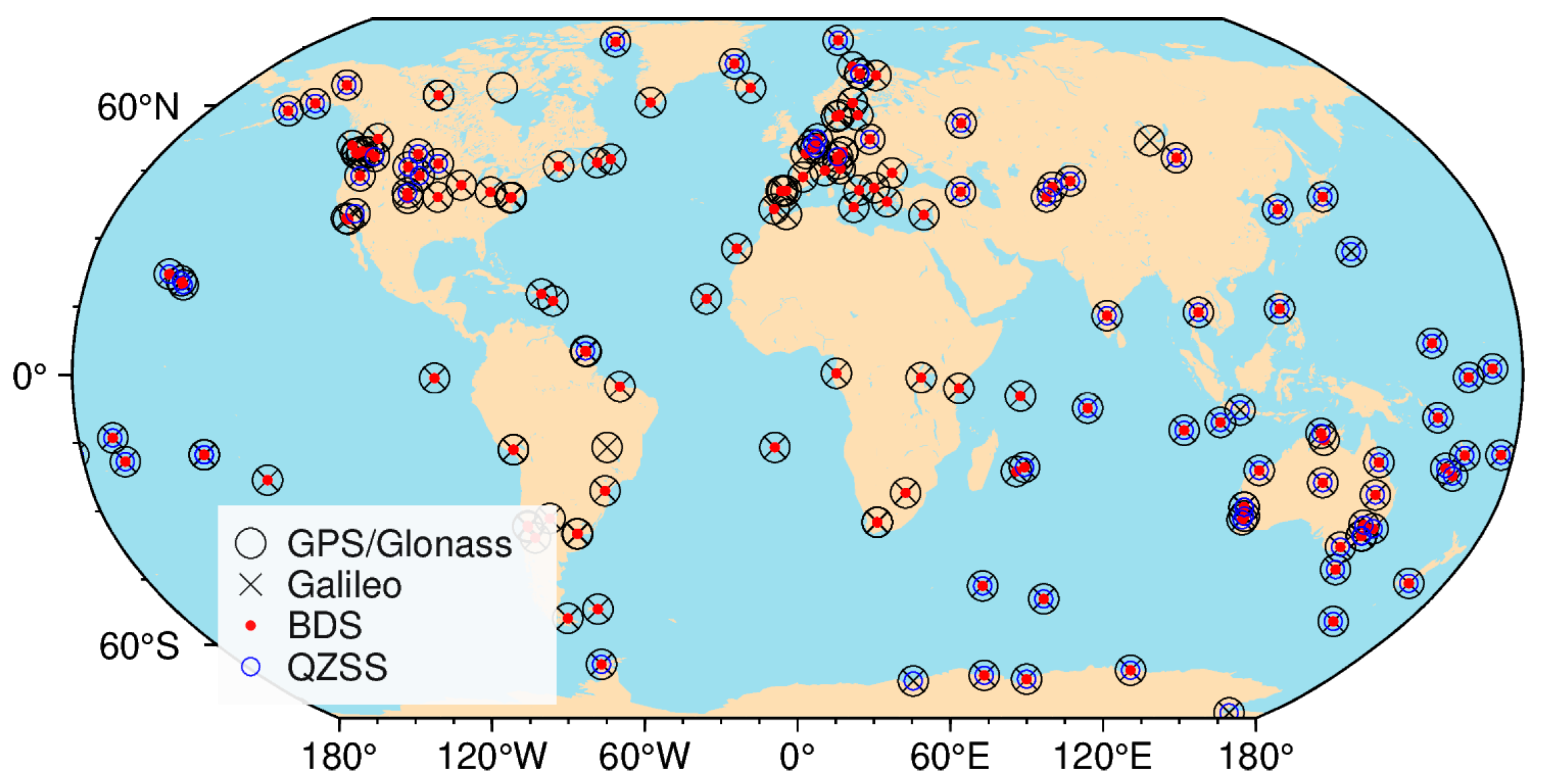
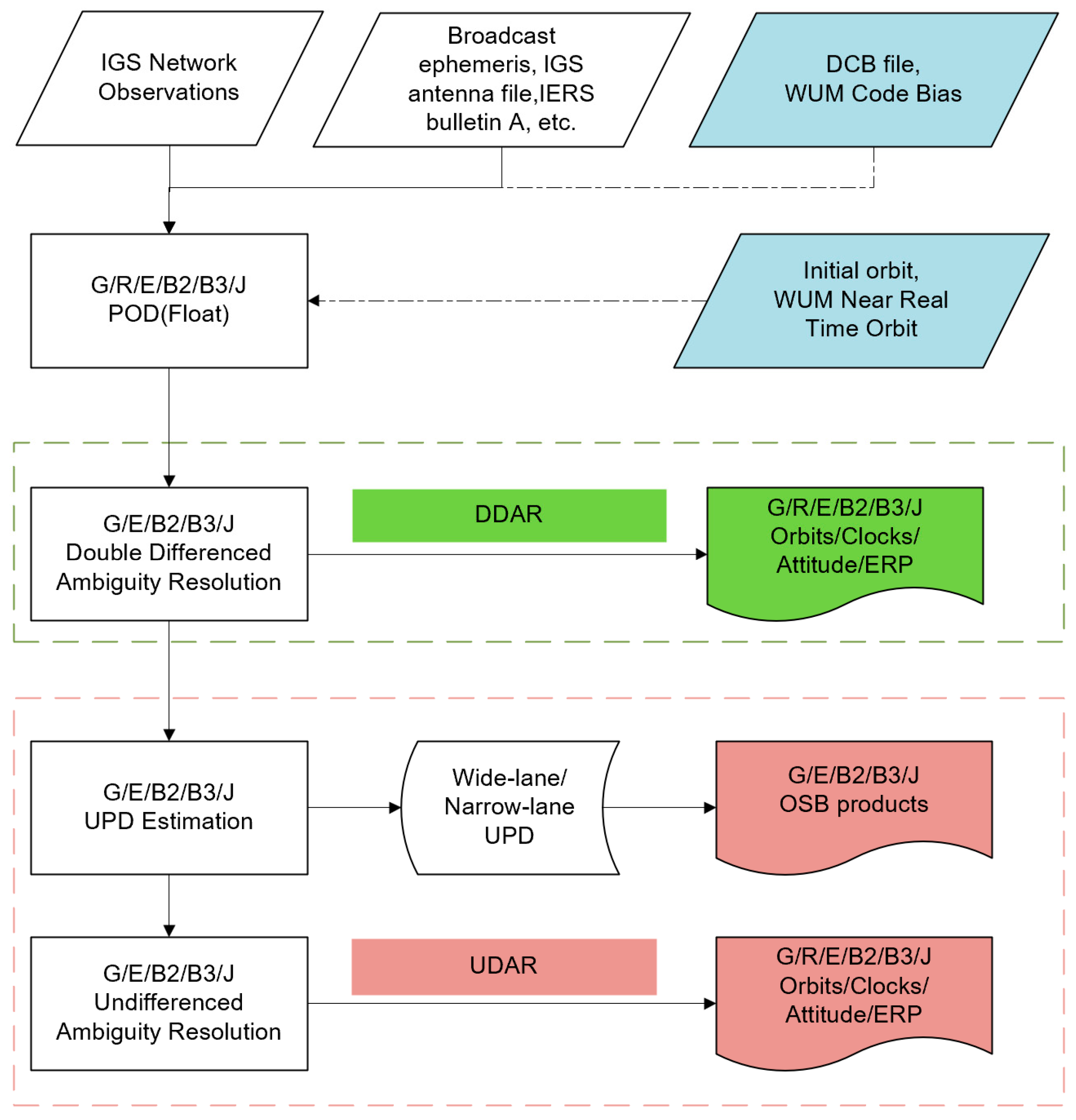
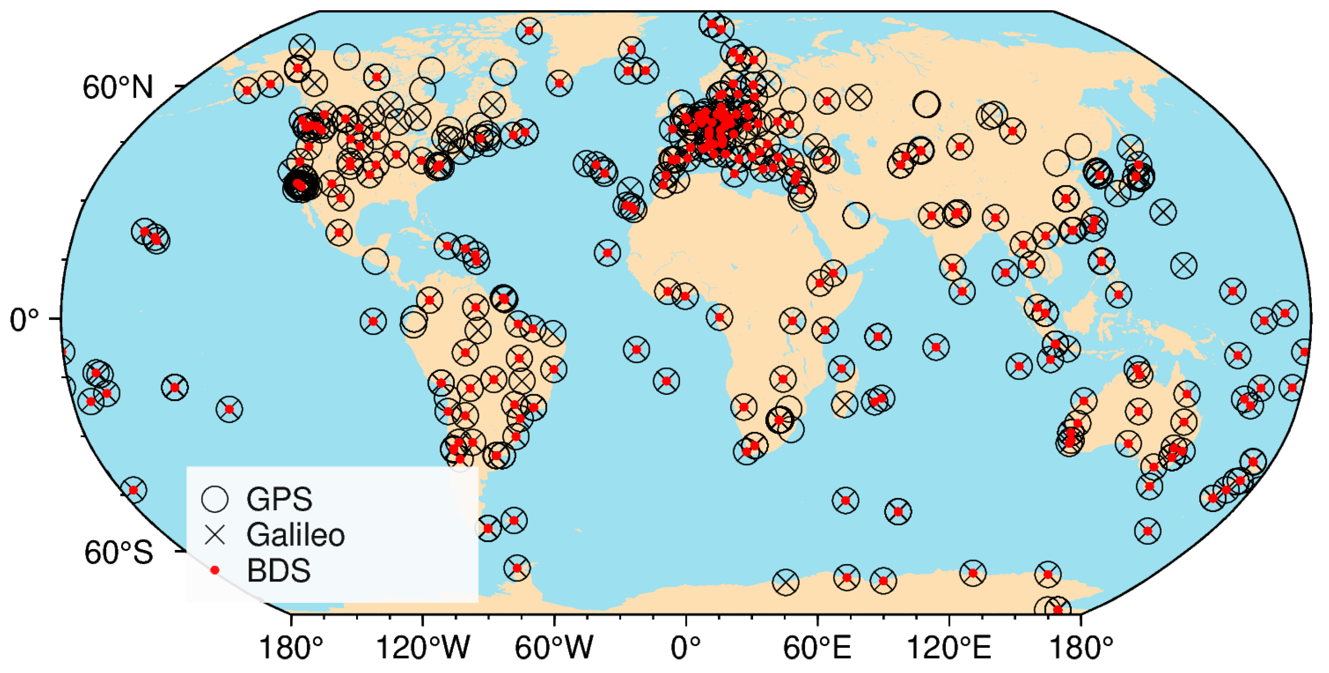
• Initial estimation: Data from six constellations—GPS, GLONASS, Galileo, BDS-2, BDS-3, and QZSS—are processed simultaneously.
• DDAR solution: Orbits, clocks, Earth rotation parameters, tropospheric delays, coordinates, and receiver clock offsets are estimated based on double-differenced ambiguity resolution. After constraining the double-differenced ambiguities, the parameters for satellites, stations, and other parameters, such as the troposphere and Earth’s rotation parameters, achieve a high level of precision. Products generated at this step are so-called IGS legacy products.
• UDAR solution: Following the DDAR solution, satellite-specific wide-lane and narrow-lane UPDs are derived using between-satellite single-difference ambiguities under a zero-mean condition. With these UPD products, undifferenced ambiguities are fixed and applied as constraints in the normal equations to obtain the final solutions. PPP-AR can be conducted based on products generated at this step.

Due to system-specific receiver code biases between BDS-2 and BDS-3’s overlapping signals (i.e., B1I/B3I), BDS-2 and BDS-3 are treated as separate constellations during data analysis and ambiguity resolution. Additionally, because GLONASS satellites utilize frequency-division multiple access technology, ambiguity resolution is not performed for these signals. Considering the strong correlation between float ionosphere-free ambiguities and clock parameters, directly fixing undifferenced ambiguities results in a relatively low fixing rate [5,13].

In our data processing approach, station coordinates are rigorously constrained to the International GNSS Service daily solutions. The raw code and phase measurement precision is set at 0.2 m and 2 mm, respectively. To mitigate the influence of low-elevation measurements, a weighting factor of 1/(2sin(Elevation Angle)) is applied, downweighting observations below 30°. Additionally, the IGS Antenna Calibration Exchange file is utilized to correct phase center variations and offsets for both receiver and satellite antennas. The station equipped with the hydrogen maser clock, offering the best data quality, serves as the time reference.

The orientation of GNSS satellites follows the conventions established by the International GNSS Service [26]. Yaw models are applied to satellites during eclipse seasons and near midnight or noon positions. Specifically, the simplified yaw models proposed by Kouba are utilized for GPS and GLONASS satellites [27,28], while the yaw model provided by the European GNSS Service Centre [29] is used for Galileo satellites. For BDS-2 satellites, models C07, C08, C09, C10, C12, and C13 employ yaw-steering and orbit normal modes [30]. The continuous yaw-steering model is applied to the remaining BDS-2 satellites. Regarding BDS-3 satellites, those manufactured by the China Academy of Space Technology (CAST) adhere to the model proposed by Wang et al. [31], whereas satellites from the Shanghai Engineering Center for Microsatellite (SECM) follow the model outlined by Yang et al. [32].

Among non-conservative perturbations, the solar radiation pressure (SRP) significantly affects GNSS satellites. The Empirical CODE Orbit Model 2 (ECOM2) has been employed [33], incorporating a priori models for GPS [34] and GLONASS [35]. Conversely, for Galileo, BDS, and Quasi-Zenith Satellite System satellites, the ECOM1 SRP model has been utilized, integrating different a priori models [25,36,37]. Additionally, Earth albedo and transmit antenna thrust effects are considered for medium Earth orbit (MEO) satellites, with transmit powers from Steigenberger et al. used for antenna thrust modeling [38]. The subroutine provided by Rodriguez-Solano et al. has been employed to model the Earth re-radiation pressure [39].

Table 1. POD strategy used for data analysis at Wuhan University.

Item	Strategy
Observable	Undifferenced ionosphere-free dual-frequency code and phase combination GPS C1P/C2P L1P/L2P GLONASS C1P/C2P L1P/L2P Galileo C1X/C5X L1X/L5X, C1C/C5Q, L1C/L5Q BDS-2 C2I/C6I L2I/L6I BDS-3 C2I/C6I L2I/L6I QZSS C1X/C2X L1X/L2X
POD arc length	24 h
Sampling rate	300 s
Elevation angle cutoff	7°
Weighting	Code: 0.2 m; phase: 2 mm Elevation-dependent weighting: E > 30°: 1; E ≤ 30°: 1/(2sin(E))
Antenna PCO/PCV	Igs20_wwww.atx for satellites and stations
Tidal displacement	Solid Earth tide [40] Ocean tide loading (FES2014b) [41] Solid Earth pole tide (FES2014b) [41]
Tropospheric delay	Global Pressure and Temperature (GPT) model with Global Mapping Function (GMF) [42]
Earth rotation	IERS Bulletin A Ocean tidal: diurnal/semidiurnal varriations applied UT1 libration applied HF EOP based on Desai model
Relativity effect	Applied based on IERS Conventions 2010
Geopotential	Earth Gravitational Model 2008 (EGM08) 12 $\times$ 12
Tidal variations in geopotential	Solid Earth tides Ocean tides Solid Earth pole tide Oceanic pole tide
Third body	Sun, Moon, Mercury, Venus, Mars, Jupiter, Saturn, Uranus, Neptune, Pluto with JPL Planetary Ephemeris 405 (DE405)
Solar radiation	GPS and GLONASS: Box-wing+ECOM2 (D, Y, B, Bc, Bs, Dc2, Ds2) [33]. Galileo: ECOM1 with a priori SRP model [36] BDS-2 GEO: 5-parameter ECOM1 with a priori SRP model [43] BDS-2 IGSO and MEO: ECOM1 with a constant parameter in the along-track direction [24] BDS-3 MEO: ECOM1 with a priori SRP model [25]
Attitude model	GPS [27]; GLONASS [28]; Galileo [29] BDS GEO: orbit nominal mode BDS-2 C07, C08, C09, C10, C12, C13: yaw-steering and orbit normal mode [30] The BDS-2 and BDS-3 MEO/IGSO CAST satellites [31] BDS-3 MEO SECM satellites [32]
Earth albedo radiation	Applied based on [39]
Satellite antenna thrust	Applied with the satellite transmit power [38] GPS: IIR-A/B 60 W, IIR-M 145 W, IIF 240 W, IIIA 300 W GLONASS: M 20–85 W, K1 105–135 W, M+ 100 W Galileo IOV: 135 W, FOC 260 W BDS-2: IGSO 185 W, MEO 130 W BDS-3: MEO-CAST 310 W, MEO-SECM 280 W QZSS: 2I 550 W, 2G 550 W, 2A 460 W
Ambiguty resolution	DDAR for GPS/Galileo/BDS-2/BDS-3/QZSS, with an additional UDAR step in the UDAR solution The tolerance of WL/NL ambiguity residuals is 0.20/0.12 cycle

Table 1. POD strategy used for data analysis at Wuhan University.

Item	Strategy
Observable	Undifferenced ionosphere-free dual-frequency code and phase combination GPS C1P/C2P L1P/L2P GLONASS C1P/C2P L1P/L2P Galileo C1X/C5X L1X/L5X, C1C/C5Q, L1C/L5Q BDS-2 C2I/C6I L2I/L6I BDS-3 C2I/C6I L2I/L6I QZSS C1X/C2X L1X/L2X
POD arc length	24 h
Sampling rate	300 s
Elevation angle cutoff	7°
Weighting	Code: 0.2 m; phase: 2 mm Elevation-dependent weighting: E > 30°: 1; E ≤ 30°: 1/(2sin(E))
Antenna PCO/PCV	Igs20_wwww.atx for satellites and stations
Tidal displacement	Solid Earth tide [40] Ocean tide loading (FES2014b) [41] Solid Earth pole tide (FES2014b) [41]
Tropospheric delay	Global Pressure and Temperature (GPT) model with Global Mapping Function (GMF) [42]
Earth rotation	IERS Bulletin A Ocean tidal: diurnal/semidiurnal varriations applied UT1 libration applied HF EOP based on Desai model
Relativity effect	Applied based on IERS Conventions 2010
Geopotential	Earth Gravitational Model 2008 (EGM08) 12 $\times$ 12
Tidal variations in geopotential	Solid Earth tides Ocean tides Solid Earth pole tide Oceanic pole tide
Third body	Sun, Moon, Mercury, Venus, Mars, Jupiter, Saturn, Uranus, Neptune, Pluto with JPL Planetary Ephemeris 405 (DE405)
Solar radiation	GPS and GLONASS: Box-wing+ECOM2 (D, Y, B, Bc, Bs, Dc2, Ds2) [33]. Galileo: ECOM1 with a priori SRP model [36] BDS-2 GEO: 5-parameter ECOM1 with a priori SRP model [43] BDS-2 IGSO and MEO: ECOM1 with a constant parameter in the along-track direction [24] BDS-3 MEO: ECOM1 with a priori SRP model [25]
Attitude model	GPS [27]; GLONASS [28]; Galileo [29] BDS GEO: orbit nominal mode BDS-2 C07, C08, C09, C10, C12, C13: yaw-steering and orbit normal mode [30] The BDS-2 and BDS-3 MEO/IGSO CAST satellites [31] BDS-3 MEO SECM satellites [32]
Earth albedo radiation	Applied based on [39]
Satellite antenna thrust	Applied with the satellite transmit power [38] GPS: IIR-A/B 60 W, IIR-M 145 W, IIF 240 W, IIIA 300 W GLONASS: M 20–85 W, K1 105–135 W, M+ 100 W Galileo IOV: 135 W, FOC 260 W BDS-2: IGSO 185 W, MEO 130 W BDS-3: MEO-CAST 310 W, MEO-SECM 280 W QZSS: 2I 550 W, 2G 550 W, 2A 460 W
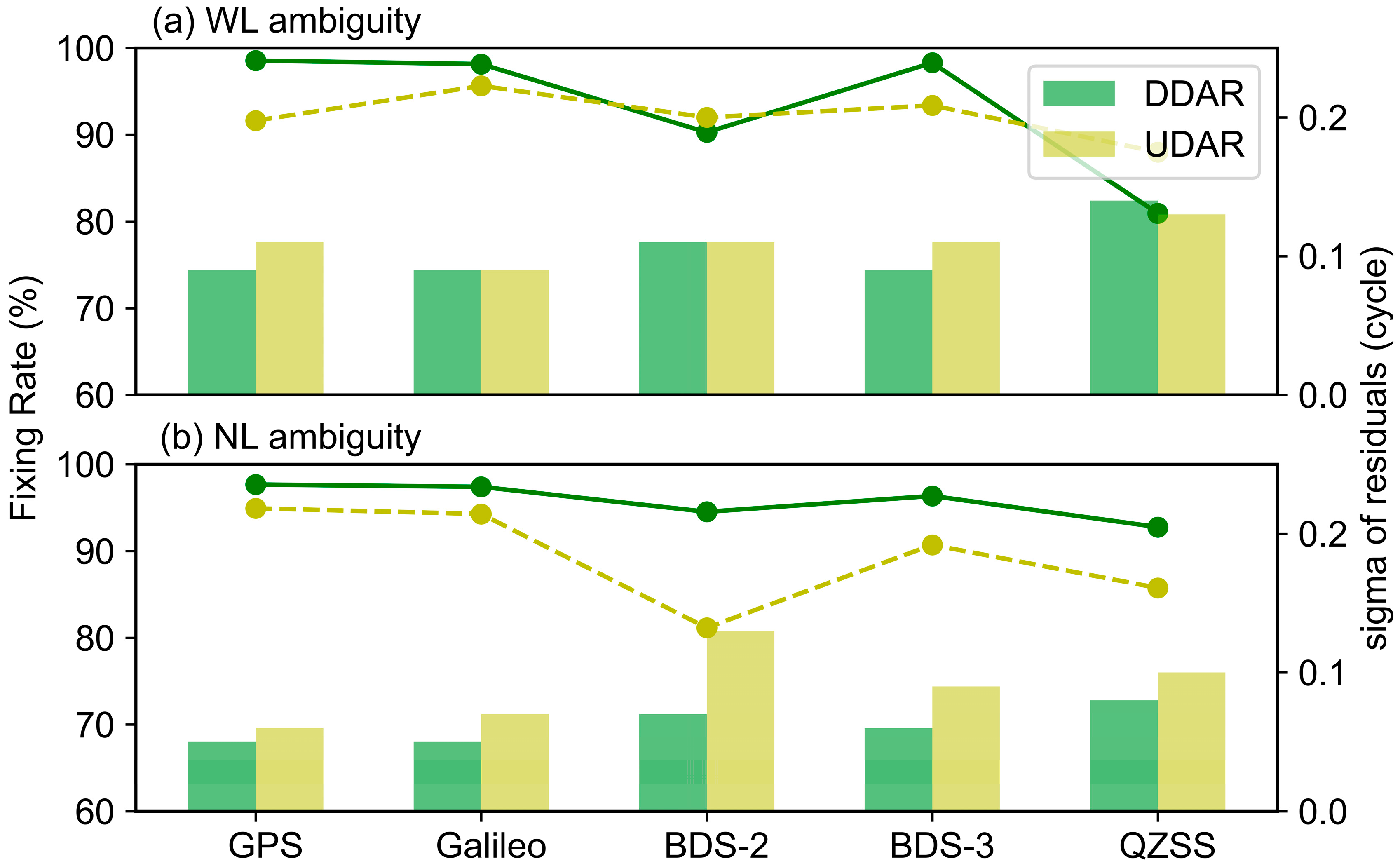
Ambiguty resolution	DDAR for GPS/Galileo/BDS-2/BDS-3/QZSS, with an additional UDAR step in the UDAR solution The tolerance of WL/NL ambiguity residuals is 0.20/0.12 cycle

4. Results

This section evaluates the impact of ambiguity resolution approaches on the performance of high-precision orbit determination products. Additionally, it analyzes the stability of observable-specific bias (OSB) products and their effects on the positioning precision.

4.1. Ambiguity Resolution

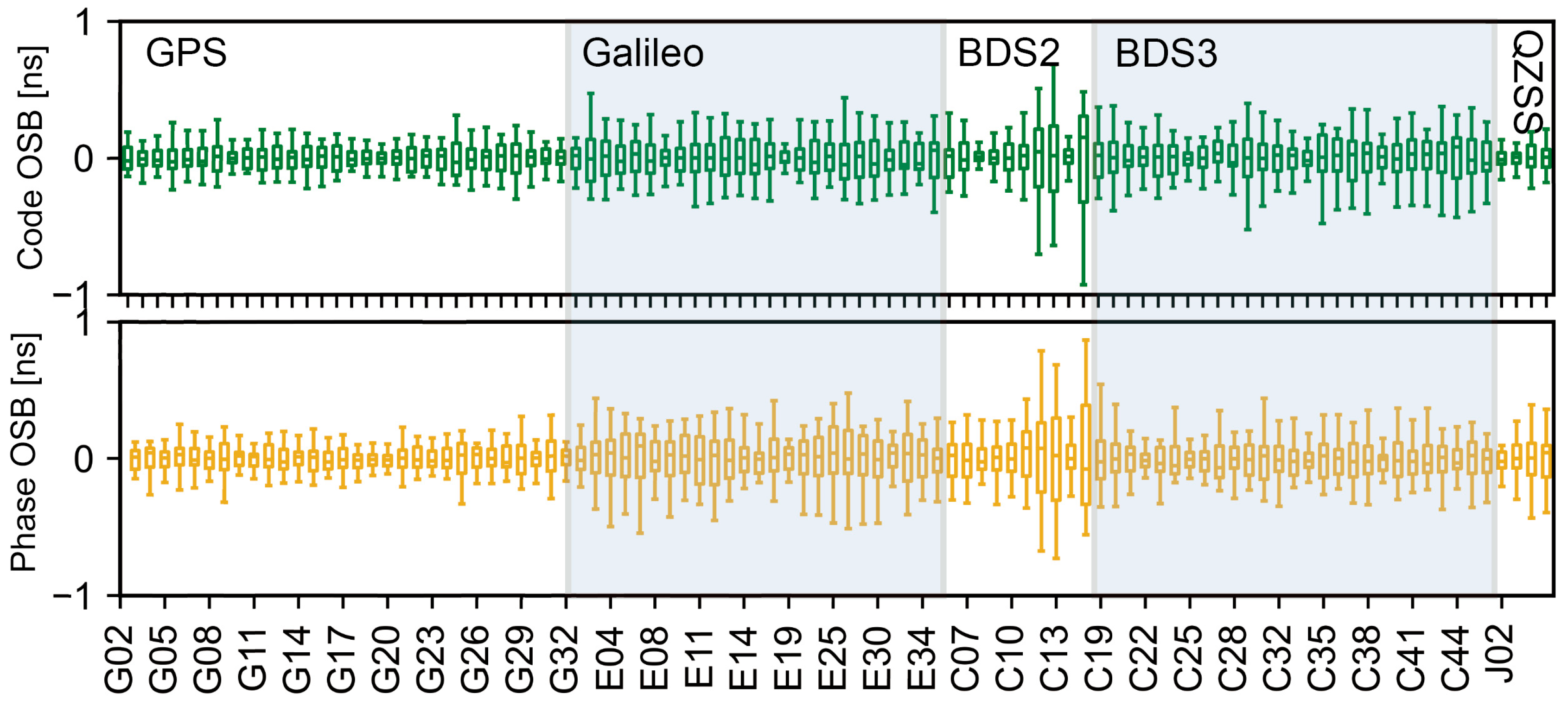
The performance of integer ambiguity resolution is evaluated using metrics such as ambiguity residuals and fixing rates for both DD and UD approaches. These metrics serve as key indicators of ambiguity resolution’s effectiveness and the quality of the estimated UPD products. Figure 3 presents the wide-lane and narrow-lane ambiguity residuals for each system, comparing both DD and UD solutions on DOY 280, 2023. Similar performance trends are observed on other days.

In general, narrow-lane residuals exhibit greater concentration compared to wide-lane residuals, particularly for GPS and Galileo systems. The larger residuals observed in WL ambiguities can be attributed to the relatively higher noise levels from Melbourne–Wübbena combinations, as code measurements are utilized. Conversely, the precision of NL ambiguities depends on ionosphere-free ambiguities, which can be precisely estimated using phase observations.

In the UDAR approach, the standard deviations (STDev) of wide-lane residuals are as follows: GPS (0.11 cycles), Galileo (0.09 cycles), BDS-2 (0.11 cycles), BDS-3 (0.11 cycles), and QZSS (0.13 cycles). Approximately 91.6%, 95.6%, 92.0%, 93.4%, and 88.0% of the WL ambiguities fall within ±0.20 cycles and can be fixed with high confidence for GPS, Galileo, BDS-2, BDS-3, and QZSS, respectively. Due to the high quality of the observations, Galileo exhibits a slightly higher fixing rate than the others, while QZSS has the lowest fixing rate, attributed to the fewer satellites deployed, followed by BDS-2 due to larger measurement noise. For narrow-lane ambiguity residuals, the averages are as follows: GPS (0.06 cycles), Galileo (0.07 cycles), BDS-2 (0.13 cycles), BDS-3 (0.09 cycles), and QZSS (0.10 cycles). Approximately 94.9%, 94.3%, 81.2%, 90.7%, and 85.7% of the NL ambiguities fall within ±0.12 cycles and can be resolved successfully for GPS, Galileo, BDS-2, BDS-3, and QZSS, respectively. Unlike the WL residuals, GPS and Galileo exhibit lower residuals due to more accurate observational error models, while BDS-2 shows poorer performance. In the DDAR approach, similar performance is observed for WL residuals among GPS, Galileo, and BDS-3, whereas QZSS and BDS-2 perform worse. Similar trends are noted for NL residuals. By eliminating common biases, the DD solution yields relatively smaller residuals and higher ambiguity fixing rates compared to the UD approach, especially for NL ambiguities. Additionally, BDS-2 exhibits relatively larger NL residuals, indicating potential unmodeled errors. This observation explains why the UDAR algorithm does not enhance the performance of BDS-2 orbits, a topic that will be discussed further in subsequent sections.

4.2. OSB Products

To enable ambiguity resolution on the user side using the undifferenced approach, it is essential to provide OSBs along with consistent satellite clock data. Wuhan University has been supplying OSB products as part of the IGS MGEX final product line since DOY 162, 2023. However, the daily products are not consistently aligned.

In this study, the OSB products are reprocessed based on a strategy similar to that used for the generation of WUM final products. However, to ensure the stability of the products, both the code OSB and wide- and narrow-lane UPDs have been aligned with the aforementioned approach. Such alignment facilitates the reduction of boundary discontinuities in the products, as well as the positioning results. Figure 4 illustrates the quality of the code and phase OSB products for the first basic frequency of each system with a box plot. OSBs with values exceeding three times the standard deviations were treated as outliers and removed. Generally, it can be clearly observed that the code OSB exhibits a more concentrated distribution for most satellites, mainly due to the phase OSB consisting of the code DCB and wide- and narrow-lane UPDs. For most satellites, the amplitude of the code OSB is within 0.5 ns, whereas it can reach up to 2 ns for the phase OSB. Among the constellations, both the code and phase OSBs of GPS show the best performance, followed by Galileo and BDS-3. The relatively lower performance of the Galileo OSB compared to GPS can be attributed to the insufficient number of Galileo C1X tracking stations during the code OSB procedure. Additionally, potential unmodeled observation errors and large noise degrade the performance of the BDS OSB, particularly for BDS-2.

4.3. Orbit

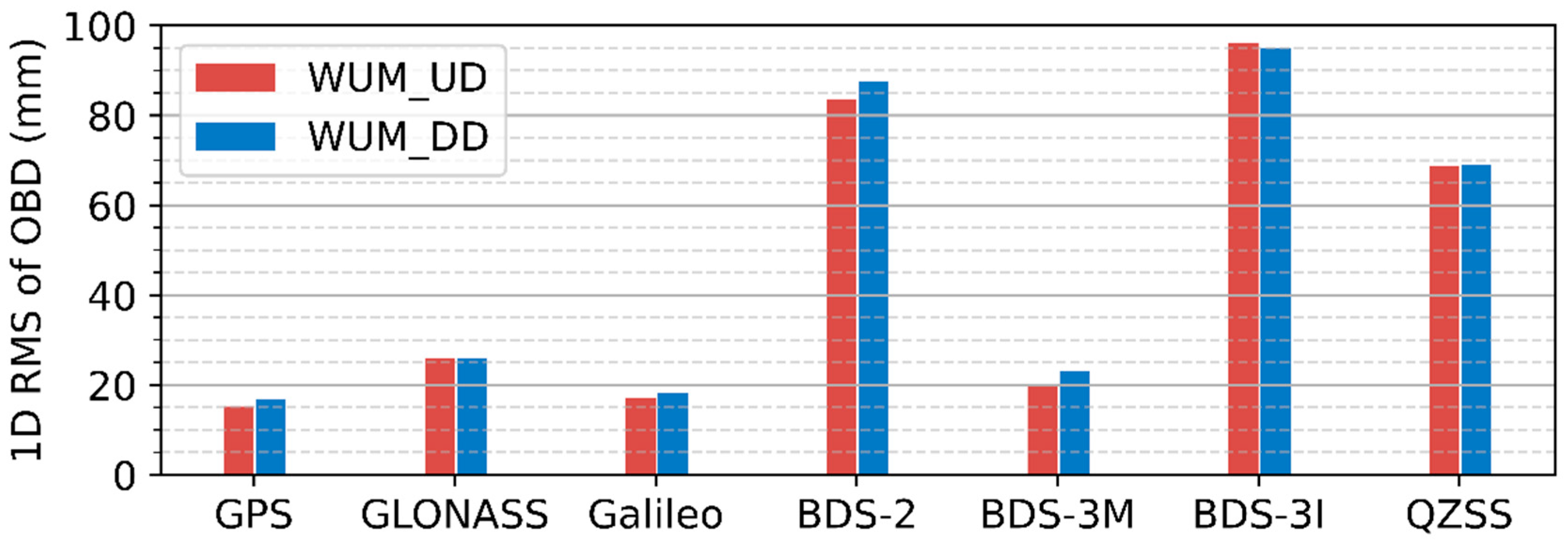
4.3.1. Orbit Boundary Discontinuity

We use the orbit boundary discontinuity (OBD) to investigate the impacts of ambiguity resolution on the orbit quality. Typically, better ambiguity resolution results in more consistent orbit solutions, thereby reducing the OBD.

Figure 5 shows the one-dimensional (1D) orbit boundary discontinuity at the midnight point for each system, based on DDAR and UDAR solutions. The values in the along-track, cross-track, and radial directions are listed in

Table 2. OBD of WUM products determined based on UD and DD strategies in along-track (A), cross-track (C), and radial directions (R) and the corresponding precision improvement rate.

Type	WUM_UD (mm)			WUM_DD (mm)			Improvement (%)
	A	C	R	A	C	R	A	C	R
GPS	16.3	13.7	15.5	18.5	15.8	16.3	11.9	13.3	4.9
GLONASS	31.8	25.8	18.3	32.1	25.8	18.4	0.9	0.0	0.5
Galileo	17.8	15.6	17.7	19.5	17.0	18.3	8.7	8.2	3.3
BDS-2	84.7	71.2	93.2	95.4	75.5	90.3	11.2	5.7	−3.2
BDS-3 MEO	21.5	18.9	19.4	25.9	22.0	21.2	17.0	14.1	8.5
BDS-3 IGSO	69.9	103.3	110.4	59.6	103.4	113.4	−17.3	0.1	2.6
QZSS	40.7	45.8	101.9	44.2	48.0	100.2	7.9	4.6	−1.7

. Noticeable differences are observed between the MEO and IGSO satellites of BDS-3, with their OBDs illustrated separately. It can be observed that there is a significant reduction in OBD for GPS, Galileo, and BDS-3 MEO satellites, with 1D RMS reductions of approximately 10.0%, 6.7%, and 13.7%, respectively. For each direction, the largest reduction is seen in the along-track case, while the smallest improvement occurs in the radial direction, as the radial orbits are dominated by the force model rather than geometric conditions. Additionally, the precision of BDS-3 IGSO in the along-track direction decreases significantly when using the UDAR approach. This may be due to the limitations of UDAR for BDS-3 IGSO, which prevent the complete elimination of unmodeled errors, leading to a deterioration in orbit precision. For GLONASS, similar performance is observed for both UDAR and DDAR solutions, as ambiguity resolution was not applied to GLONASS in this study.

4.3.2. Comparison with Other Products

By using the IGS and ESA’s final multi-GNSS solutions as references, the orbit products from all IGS MGEX ACs, as well as our DD and UD orbit solutions, are assessed. For GPS and GLONASS, the IGS final orbits are used as the reference, while the ESA MGEX final solution serves as the reference for the other systems. To eliminate inconsistencies between the solutions, a seven-parameter Helmert transformation is applied. Additionally, orbit errors exceeding five times the RMS are removed. As a result, 0.9–3.4% of all solutions are discarded from each AC’s orbit products. Figure 6 shows the time series of the daily RMS orbit differences, with the corresponding statistical results listed in

Table 3. The 1D RMS of orbit differences between different AC solutions with respect to that of the IGS or ESA (unit: mm).

	GPS	Galileo	GLONASS	BDS-2 (MEO)	BDS-2 (IGSO/GEO)	BDS-3 (MEO)	BDS-3 (IGSO)	QZSS
WUM_UD	9.1	12.4	31.2	73.7	86.3	20.1	98.5	71.8
WUM_DD	9.8	13.7	31.2	74.2	86.7	23.7	93.8	71.2
COM	10.1	13.1	32.8	60.0	113.4	25.8	118.5	77.5
GBM	11.4	14.5	38.8	75.8	100.4	28.1	112.2	103.7
GRG	11.2	14.4	36.9	/	/	/	/	/
JAX	11.6	15.4	31.7	/	/	/	/	82.5
IAC	12.7	14.9	34.4	38.6	62.9	25.6	123.3	95.7

.

It can be observed that the GPS and Galileo orbits from all ACs show good consistency, followed by the BDS-3 and GLONASS satellites, likely due to the similar strategies employed by the ACs for GPS and Galileo data analysis. For GLONASS, the relatively large differences arise from float ambiguity resolution. For BDS-3 MEO satellites, the consistency between different orbit solutions is worse than for GPS and Galileo, likely due to fewer tracking stations and potential observation errors, which further degrade the orbit quality of BDS-2 MEO satellites. Due to the poorer observation geometry and the solar radiation pressure model, the IGSO and GEO satellites of BDS and QZSS exhibit the worst consistency among all satellites.

The orbits of GPS and Galileo from all ACs show good consistency, followed by those of BDS-3 and GLONASS, likely due to the similar strategies used by the ACs for GPS and Galileo data analysis. For GLONASS, the relatively large differences are attributed to float ambiguity resolution. For BDS-3 MEO satellites, the consistency between different orbit solutions is worse than for GPS and Galileo, likely due to fewer tracking stations and potential observation errors, which further degrade the orbit quality of BDS-2 MEO satellites. Due to the poorer observation geometry and the solar radiation pressure model, the IGSO and GEO satellites of BDS, as well as QZSS, exhibit the worst consistency among all satellites.

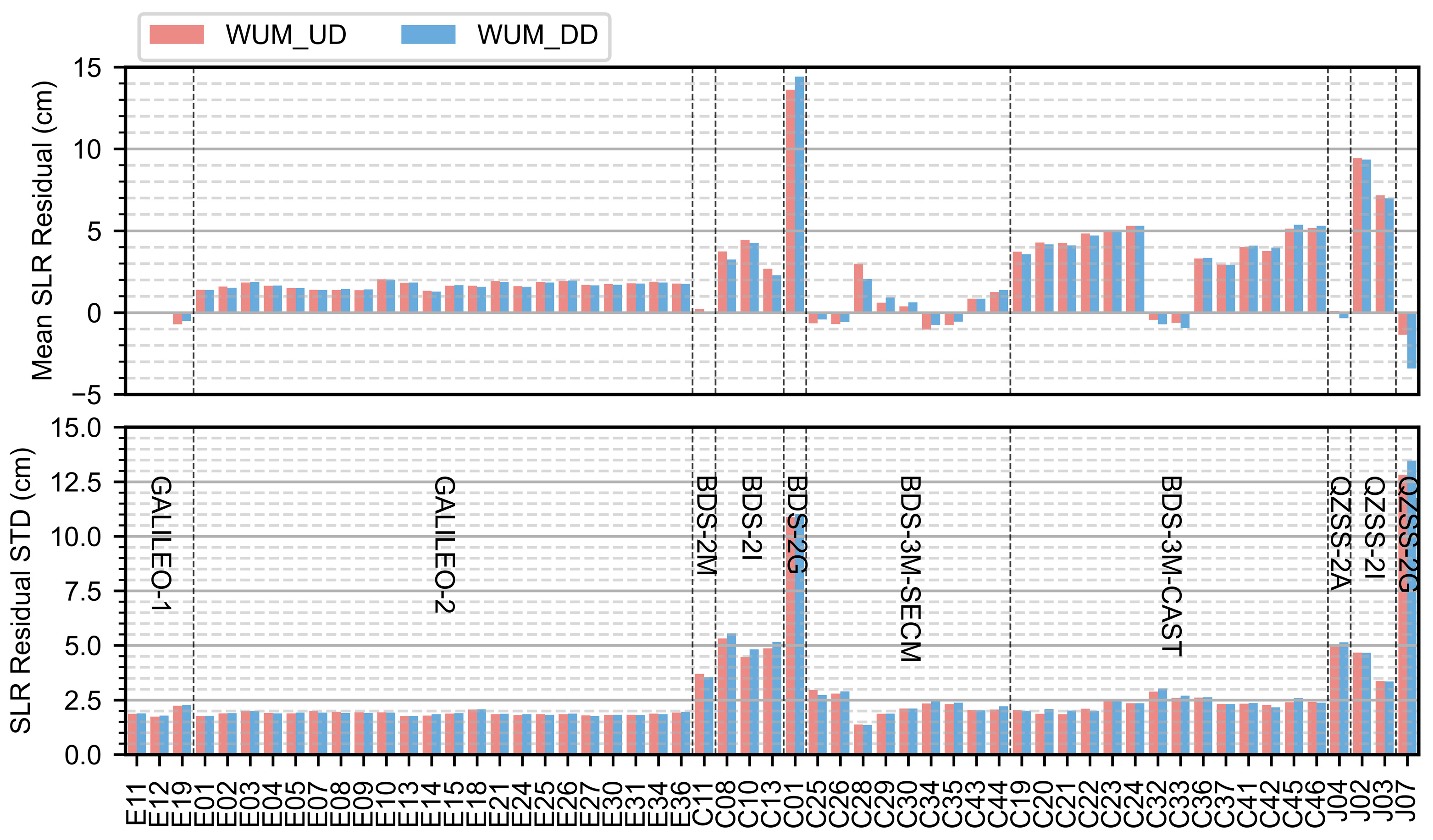
4.3.3. Satellite Laser Ranging Validation

SLR can measure the distance between ground stations and satellites with centimeter-level precision, making it a useful tool in assessing the absolute orbit precision of GNSS satellites. Figure 7 presents the statistical results of the SLR residuals for the DD and UD orbit solutions of Galileo, BDS-3, and BDS-2 satellites in 2023. Residuals exceeding five times the RMS were removed, resulting in the removal of 0–3% of all data used for evaluation.

The mean SLR residuals for Galileo in-orbit validation (IOV) satellites are close to 0, while the mean value for full-orbit-capacity (FOC) satellites is 1.7 cm. BDS-2 GEO satellites exhibit a larger bias of 13.6 cm, whereas BDS-2 IGSO satellites show a deviation of 3.6 cm, and the bias for BDS-2 MEO satellites is also close to 0. BDS-3-SECM satellites demonstrate good consistency, with an overall bias near 0, while CAST satellites exhibit a bias of around 3.6 cm, likely due to the inaccurate offset of the laser array with respect to the center of mass. The overall biases for QZSS-2A/GEO/IGSO satellites are 0.1/−1.4/8.3 cm. No significant change is observed after adopting the UDAR strategy.

The STDev of the SLR residuals for the UDAR solution of Galileo IOV satellites is 1.9 cm, representing a 2.1% improvement compared to the DDAR solution. For Galileo FOC satellites, both solutions achieve similar precision of 1.8 cm. For BDS-2 MEO satellites, the STDev of the SLR residuals for the UD solution is 3.7 cm, showing slight degradation (about 4.6%) compared to the DDAR solution. A 4.3% improvement is observed for BDS-2 IGSO satellites when using the UDAR ambiguity approach. No changes are observed for GEO satellites, with an STDev of about 10.9 cm for both solutions. For BDS-3 satellites, the STDev of the SLR residuals is 2.3 cm for both solutions, while, for QZSS-2A, QZSS-2 IGSO, and QZSS-2 GEO satellites, the STDev is 5.1 cm, 4.0 cm, and 12.8 cm, respectively. The improvements are 0.9%, 0.3%, and 4.8%, compared to the DDAR solution.

Overall, the orbit precision has been improved slightly, as shown by the SLR validation; this demonstrates that the impact of ambiguity resolution on the radial orbit precision is limited, as it is mainly dominated by the force perturbation.

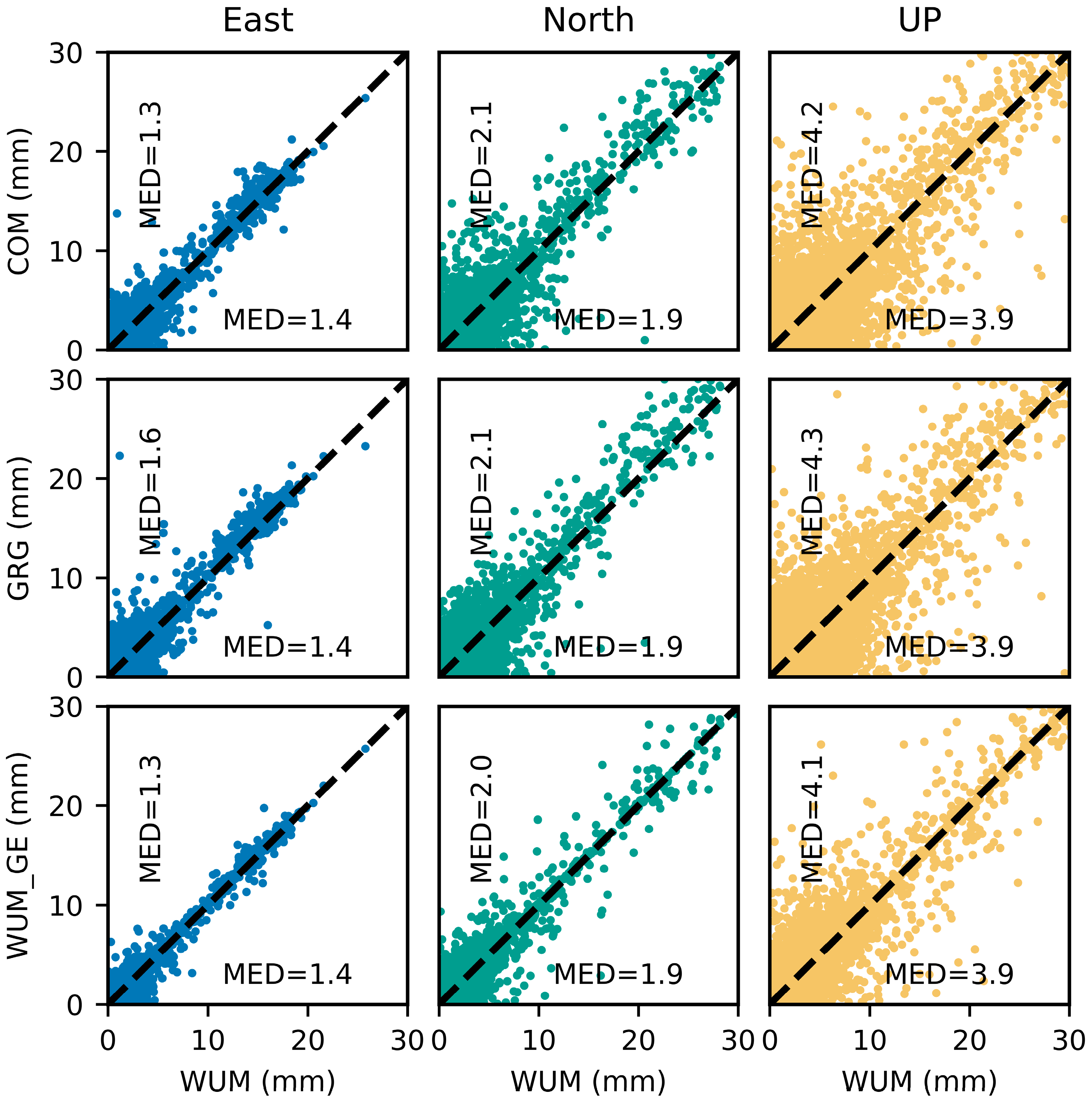
4.4. Global Multi-GNSS PPP-AR

To validate the quality and consistency of the orbit, clock, and OSB products, PPP was performed in both static and kinematic modes for approximately 430 global IGS stations using the open-source software PRIDE PPP-AR ver 3.0 [44]. All stations can track GPS signals, while 358 and 301 stations are capable of tracking Galileo and BDS signals, respectively. Data from the entire month of October 2023 were selected, and the MGEX products from CODE (COM) and CNES/CLS (GRG) were processed for comparison. For the WUM solution, GPS, Galileo, BDS-2, and BDS-3 data were processed simultaneously. Since only GPS and Galileo OSB products are available from COM and GRG, PPP-AR was conducted for GPS and Galileo using these products. For comparison, additional PPP-AR for GPS/Galileo was conducted using the WUM products (WUM_GE). Figure 8 shows the global distribution of ground stations on 1 October 2023. It can be observed that many receivers are located in Europe and North America. Specifically, there are 60, 122, 59, and 44 stations equipped with Septentrio, Trimble, Javad, and Leica receivers, while the remaining stations consist of 19 Novtel, 14 TPS, 5 ASHTECH, 3 JPS, 2 STONEX, and 1 CHC.

Among the 430 stations, 398 were selected for validation as their data were complete for at least 27 days during the study period. Additionally, stations with a GPS ambiguity fixing rate of less than 50% were excluded from the validation, leaving 394 stations for analysis.

Table 4. WL and NL ambiguity fixing rates for the static PPP-AR solutions with WUM/COM/GRG products, as percentages.

AC	GPS	Galileo	BDS-2	BDS-3
WUM	90.3/99.2	97.2/99.2	87.4/88.8	91.1/98.6
COM	90.6/99.0	97.5/98.7
GRG	90.8/95.2	95.5/98.2
WUM_GE	90.3/99.1	97.2/99.2

lists the ambiguity fixing rates for the PPP-AR solutions using different products. It can be observed that the GPS wide-lane fixing rate for WUM is slightly lower than that of the others. This is mainly due to the lower performance of ambiguity fixing for Trimble receivers based on the WUM solution, which requires further investigation. For GPS, the narrow-lane fixing rate nearly reaches 100%, indicating good consistency between the orbit, clock, and OSB products. Finally, the fixing rates are 89.6%, 89.7%, and 86.5% for the WUM, COM, and GRG solutions, respectively.

For Galileo, due to the high quality of the observations, particularly the code measurements, a relatively high wide-lane ambiguity fixing rate can be achieved compared to GPS and BDS. For WUM, the fixing rate is 97.2%, while it is approximately 97.5% and 95.5% for the COM and GRG solutions, respectively. Similarly to GPS, the narrow-lane fixing rate reaches nearly 100%. Since the receiver can only receive either C/Q or X/X signals from Galileo, there are no overlapping stations to solve them simultaneously. To address this issue, COM estimates the OSB from these signals independently, while WUM and GRG treat the biases as the same for these signals. By comparing the ambiguity fixing rates of GRG with those of COM and WUM, it is evident that the differences in the wide-lane fixing rates between GRG and COM are smaller, with the narrow-lane fixing rate difference being less than 0.5%. However, the ambiguity fixing rates for both wide-lane and narrow-lane cases for WUM are close to those of COM. Therefore, we conclude that the discrepancy between the Galileo C/Q and X/X OSBs is negligible for PPP-AR.

As COM and GRG did not release the OSB products for BDS during this period, only WUM is used for validation. It can be observed that BDS-3 exhibits similar performance to GPS, as indicated by the ambiguity fixing rate. However, the fixing rate for BDS-2 is lower, particularly for the narrow lane, which can be attributed to the relatively lower precision of BDS-2’s orbit and clock, due to fewer tracking stations and unmodeled observation errors.

The repeatability of positioning in the north, east, and vertical (up) components is used as a reliable quality measure for the validation of static PPP-AR. The precision of the PPP-AR solutions from different ACs is presented in Figure 9. For comparison, a seven-parameter Helmert transformation is applied to remove systematic errors. In general, the GRG solution shows slightly lower performance than COM and WUM, particularly in the east direction, as its precision is more sensitive to integer ambiguity resolution. The median daily repeatability for WUM is 1.4 mm, 1.9 mm, and 3.9 mm in the east, north, and up directions, respectively. Compared to COM, the points are nearly aligned along the diagonal line, indicating that the PPP-AR performance of both solutions is quite similar.

By comparing the WUM and WUM_GE solutions, we found that the absence of BDS-2 and BDS-3 led to a slight decrease in the narrow-lane fixing rate of GPS in the static PPP-AR solution, and the precision in the vertical direction increased from 3.9 mm to 4.1 mm.

5. Conclusions and Outlook

This study summarizes the strategy routinely used to generate the WUM final products based on the undifferenced ambiguity resolution method. The impact of the UDAR method on precise orbit determination is discussed using metrics of orbit consistency and SLR validation. Furthermore, the stability of pseudorange OSB and phase OSB products is examined, and these products are validated using PPP-AR in comparison to those from other ACs.

Among all GNSS systems, GPS and Galileo exhibit the highest orbit precision. WUM’s implementation of the undifferenced ambiguity resolution strategy results in improvements in the RMS values, with a 7.1% reduction to 9.1 mm for GPS and a 9.5% reduction to 12.4 mm for Galileo. For BDS-3 MEO satellites, a 15.2% improvement, reducing the RMS to 20.1 mm, is achieved over the DDAR solution. For BDS-2 MEO satellites, a minimal 1.0% reduction in the RMS to 73.7 mm is observed. BDS-3 IGSO and BDS-2 GEO satellites show relatively lower precision, with RMS values of 37.0 mm and 84.3 mm, respectively. The QZSS satellite orbit precision reaches 72.0 mm, with minimal variations among different solutions. Despite the increased number of fixed ambiguities, the impact on the radial orbit precision remains limited, as it is predominantly influenced by the force model. Consequently, only a limited improvement is observed in the SLR residuals.

The validation of the WUM products is conducted through GPS, Galileo, BDS-2, and BDS-3 combined PPP-AR, involving 480 globally distributed stations. For static PPP-AR, the fixing rates for these systems reach 89.6%, 96.4%, 78.5%, and 89.9%, respectively. The median daily repeatability of WUM is 1.4 mm, 1.9 mm, and 3.9 mm in the east, north, and up directions, respectively. For kinematic PPP-AR, the narrow-lane fixing rates for WUM are the highest among all analysis center products—specifically 93.7%, 96.0%, 79.9%, and 93.7%. These results confirm the high quality of the WUM final products and the benefits of undifferenced ambiguity resolution in generating consistent orbit, clock, and bias products.

References

1. Blewitt, G. Carrier phase ambiguity resolution for the Global Positioning System applied to geodetic baselines up to 2000 km. J. Geophys. Res. Solid Earth 1989, 94, 10187–10203. [Google Scholar] [CrossRef]
2. Dong, D.-N.; Bock, Y. Global Positioning System Network analysis with phase ambiguity resolution applied to crustal deformation studies in California. J. Geophys. Res. Solid Earth 1989, 94, 3949–3966. [Google Scholar] [CrossRef]
3. Ge, M.; Gendt, G.; Dick, G.; Zhang, F.P.; Rothacher, M. A New Data Processing Strategy for Huge GNSS Global Networks. J. Geod. 2006, 80, 199–203. [Google Scholar] [CrossRef]
4. Ge, M.; Gendt, G.; Rothacher, M.; Shi, C.; Liu, J. Resolution of GPS carrier-phase ambiguities in Precise Point Positioning (PPP) with daily observations. J. Geod. 2008, 82, 389–399. [Google Scholar] [CrossRef]
5. Geng, J.; Shi, C.; Ge, M.; Dodson, A.H.; Lou, Y.; Zhao, Q.; Liu, J. Improving the estimation of fractional-cycle biases for ambiguity resolution in precise point positioning. J. Geod. 2012, 86, 579–589. [Google Scholar] [CrossRef]
6. Laurichesse, D.; Mercier, F.; Berthias, J.-P.; Broca, P.; Cerri, L. Integer Ambiguity Resolution on Undifferenced GPS Phase Measurements and Its Application to PPP and Satellite Precise Orbit Determination. Navigation 2009, 56, 135–149. [Google Scholar] [CrossRef]
7. Collins, P.; Bisnath, S.; Lahaye, F.; Héroux, P. Undifferenced GPS Ambiguity Resolution Using the Decoupled Clock Model and Ambiguity Datum Fixing. Navigation 2010, 57, 123–135. [Google Scholar] [CrossRef]
8. Geng, J.; Meng, X.; Dodson, A.H.; Teferle, F.N. Integer ambiguity resolution in precise point positioning: Method comparison. J. Geod. 2010, 84, 569–581. [Google Scholar] [CrossRef]
9. Shi, J.; Gao, Y. A comparison of three PPP integer ambiguity resolution methods. GPS Solut. 2014, 18, 519–528. [Google Scholar] [CrossRef]
10. Banville, S.; Geng, J.; Loyer, S.; Schaer, S.; Springer, T.; Strasser, S. On the interoperability of IGS products for precise point positioning with ambiguity resolution. J. Geod. 2020, 94, 10. [Google Scholar] [CrossRef]
11. Bertiger, W.; Desai, S.D.; Haines, B.; Harvey, N.; Moore, A.W.; Owen, S.; Weiss, J.P. Single receiver phase ambiguity resolution with GPS data. J. Geod. 2010, 84, 327–337. [Google Scholar] [CrossRef]
12. Teunissen, P.J.G.; Khodabandeh, A. Review and principles of PPP-RTK methods. J. Geod. 2015, 89, 217–240. [Google Scholar] [CrossRef]
13. Deng, Z.; Wang, J.; Ge, M. The GBM Rapid Product and the Improvement from Undifferenced Ambiguity Resolution. In Proceedings of the EGU General Assembly 2022, Vienna, Austria, 23–27 May 2022. [Google Scholar] [CrossRef]
14. Chen, H.; Jiang, W.; Ge, M.; Wickert, J.; Schuh, H. An enhanced strategy for GNSS data processing of massive networks. J. Geod. 2014, 88, 857–867. [Google Scholar] [CrossRef]
15. Geng, J.; Mao, S. Massive GNSS Network Analysis Without Baselines: Undifferenced Ambiguity Resolution. J. Geophys. Res. Solid Earth 2021, 126, e2020JB021558. [Google Scholar] [CrossRef]
16. Johnston, G.; Riddell, A.; Hausler, G. The International GNSS Service. In Springer Handbook of Global Navigation Satellite Systems; Teunissen, P.J.G., Montenbruck, O., Eds.; Springer International Publishing: Cham, Switzerland, 2017; pp. 967–982. ISBN 978-3-319-42928-1. [Google Scholar]
17. Schaer, S.; Villiger, A.; Arnold, D.; Dach, R.; Prange, L.; Jäggi, A. The CODE ambiguity-fixed clock and phase bias analysis products: Generation, properties, and performance. J. Geod. 2021, 95, 81. [Google Scholar] [CrossRef]
18. Strasser, S.; Mayer-Gürr, T.; Zehentner, N. Processing of GNSS constellations and ground station networks using the raw observation approach. J. Geod. 2019, 93, 1045–1057. [Google Scholar] [CrossRef]
19. Geng, J.; Zhang, Q.; Li, G.; Liu, J.; Liu, D. Observable-specific phase biases of Wuhan multi-GNSS experiment analysis center’s rapid satellite products. Satell. Navig. 2022, 3, 23. [Google Scholar] [CrossRef]
20. Geng, J.; Chen, X.; Pan, Y.; Zhao, Q. A modified phase clock/bias model to improve PPP ambiguity resolution at Wuhan University. J. Geod. 2019, 93, 2053–2067. [Google Scholar] [CrossRef]
21. Ge, M.; Gendt, G.; Dick, G.; Zhang, F.P. Improving carrier-phase ambiguity resolution in global GPS network solutions. J. Geod. 2005, 79, 103–110. [Google Scholar] [CrossRef]
22. Wang, N.; Li, Z.; Duan, B.; Hugentobler, U.; Wang, L. GPS and GLONASS observable-specific code bias estimation: Comparison of solutions from the IGS and MGEX networks. J. Geod. 2020, 94, 74. [Google Scholar] [CrossRef]
23. Liu, J.; Ge, M. PANDA software and its preliminary result of positioning and orbit determination. Wuhan Univ. J. Nat. Sci. 2003, 8, 603–609. [Google Scholar] [CrossRef]
24. Guo, J.; Xu, X.; Zhao, Q.; Liu, J. Precise orbit determination for quad-constellation satellites at Wuhan University: Strategy, result validation, and comparison. J. Geod. 2016, 90, 143–159. [Google Scholar] [CrossRef]
25. Guo, J.; Wang, C.; Chen, G.; Xu, X.; Zhao, Q. BDS-3 precise orbit and clock solution at Wuhan University: Status and improvement. J. Geod. 2023, 97, 15. [Google Scholar] [CrossRef]
26. Montenbruck, O.; Schmid, R.; Mercier, F.; Steigenberger, P.; Noll, C.; Fatkulin, R.; Kogure, S.; Ganeshan, A.S. GNSS satellite geometry and attitude models. Adv. Space Res. 2015, 56, 1015–1029. [Google Scholar] [CrossRef]
27. Kouba, J. A simplified yaw-attitude model for eclipsing GPS satellites. GPS Solut. 2009, 13, 1–12. [Google Scholar] [CrossRef]
28. Kouba, J. A Note on the December 2013 Version of the eclips.f Subroutine. Available online: http://acc.igs.org/orbits/eclipsDec2013note.pdf (accessed on 4 February 2024).
29. GSA. Galileo Satellite Metadata. 2021. Available online: https://www.gsc-europa.eu/support-to-developers/galileo-satellite-metadata (accessed on 28 November 2021).
30. Zhao, Q.; Wang, C.; Guo, J.; Wang, B.; Liu, J. Precise orbit and clock determination for BeiDou-3 experimental satellites with yaw attitude analysis. GPS Solut. 2018, 22, 4. [Google Scholar] [CrossRef]
31. Wang, C.; Guo, J.; Zhao, Q.; Liu, J. Yaw attitude modeling for BeiDou I06 and BeiDou-3 satellites. GPS Solut. 2018, 22, 117. [Google Scholar] [CrossRef]
32. Yang, C.; Guo, J.; Zhao, Q. Yaw attitudes for BDS-3 IGSO and MEO satellites: Estimation, validation and modeling with intersatellite link observations. J. Geod. 2023, 97, 6. [Google Scholar] [CrossRef]
33. Arnold, D.; Meindl, M.; Beutler, G.; Dach, R.; Schaer, S.; Lutz, S.; Prange, L.; Sośnica, K.; Mervart, L.; Jäggi, A. CODE’s new solar radiation pressure model for GNSS orbit determination. J. Geod. 2015, 89, 775–791. [Google Scholar] [CrossRef]
34. Duan, B.; Hugentobler, U. Enhanced solar radiation pressure model for GPS satellites considering various physical effects. GPS Solut. 2021, 25, 42. [Google Scholar] [CrossRef]
35. Duan, B.; Hugentobler, U.; Hofacker, M.; Selmke, I. Improving solar radiation pressure modeling for GLONASS satellites. J. Geod. 2020, 94, 72. [Google Scholar] [CrossRef]
36. Montenbruck, O.; Steigenberger, P.; Hugentobler, U. Enhanced solar radiation pressure modeling for Galileo satellites. J. Geod. 2015, 89, 283–297. [Google Scholar] [CrossRef]
37. Zhao, Q.; Chen, G.; Guo, J.; Liu, J.; Liu, X. An a priori solar radiation pressure model for the QZSS Michibiki satellite. J. Geod. 2018, 92, 109–121. [Google Scholar] [CrossRef]
38. Steigenberger, P.; Thoelert, S.; Montenbruck, O. GNSS satellite transmit power and its impact on orbit determination. J. Geod. 2018, 92, 609–624. [Google Scholar] [CrossRef]
39. Rodriguez-Solano, C.J.; Hugentobler, U.; Steigenberger, P.; Lutz, S. Impact of Earth radiation pressure on GPS position estimates. J. Geod. 2012, 86, 309–317. [Google Scholar] [CrossRef]
40. Petit, G.; Luzum, B. The IERS Conventions 2010; No. 36 in IERS Technical Note; Verlag des Bundesamtes für Kartographie und Geodäsie: Frankfurt am Main, Germany, 2010. [Google Scholar]
41. Lyard, F.H.; Allain, D.J.; Cancet, M.; Carrère, L.; Picot, N. FES2014 global ocean tides atlas: Design and performances. Ocean Sci. 2020, 17, 615–649. [Google Scholar] [CrossRef]
42. Boehm, J.; Heinkelmann, R.; Schuh, H. Short note: A global model of pressure and temperature for geodetic applications. J. Geod. 2007, 81, 679–683. [Google Scholar] [CrossRef]
43. Wang, C.; Guo, J.; Zhao, Q.; Liu, J. Empirically derived model of solar radiation pressure for BeiDou GEO satellites. J. Geod. 2019, 93, 791–807. [Google Scholar] [CrossRef]
44. Geng, J.; Yang, S.; Guo, J. Assessing IGS GPS/Galileo/BDS-2/BDS-3 phase bias products with PRIDE PPP-AR. Satell. Navig. 2021, 2, 17. [Google Scholar] [CrossRef]
Figure 1. The distribution of stations used for POD processing at 1 October 2023.
Remotesensing 17 01451 g001
Figure 2. The workflow for the data analysis based on undifferenced ambiguity resolution at Wuhan University. G/R/E/B2/B3/J represents GPS, GLONASS, BDS-2, BDS-3, and QZSS.
Remotesensing 17 01451 g002
Figure 3. The wide-lane (a) and narrow-lane (b) ambiguity fixing rates, as well as the residuals, for double-differenced and undifferenced ambiguity resolution.
Remotesensing 17 01451 g003
Figure 4. Stability of code OSB (top) and phase OSB (bottom) for GPS C1W/L1W, Galileo C1X/L1X, BDS C2I/L2I, and QZSS C1X/L1X. Please note that the mean values have been removed.
Remotesensing 17 01451 g004
Figure 5. OBD of WUM products generated based on UD and DD strategies.
Remotesensing 17 01451 g005
Figure 6. Daily 1D RMS of orbit differences with respect to IGS products for GPS as well as GLONASS and ESA MGEX products for other systems from DOY 330, 2022 to DOY 330, 2023.
Remotesensing 17 01451 g006
Figure 7. Mean (up) and STD (bottom) values of SLR residuals for orbit solutions based on DD and UD ambiguity resolution approaches.
Remotesensing 17 01451 g007
Figure 8. The distribution of stations used for PPP-AR processing at 1 October 2023.
Remotesensing 17 01451 g008
Figure 9. Ambiguity-fixed position RMS comparison between the daily PPP-AR solutions based on the COM, GRG, and WUM phase bias products.
Remotesensing 17 01451 g009