An Improved Fading Factor-Based Adaptive Robust Filtering Algorithm for SINS/GNSS Integration with Dynamic Disturbance Suppression

Abstract

Aiming at the problem of nonlinear observation model mismatch and insufficient anti-interference ability of SINS/GNSS integrated navigation system in complex dynamic environment, this paper proposes an adaptive robust filtering algorithm with improved fading factor. Aiming at the problem that the traditional Kalman filter is easy to diverge in severe heave motion and abnormal observation, a multi-source information fusion framework integrating satellite positioning geometric accuracy factor (PDOP), solution quality factor (Q value), effective satellite observation number (Satnum), and residual vector is constructed. The dynamic weight adjustment mechanism is designed to realize the real-time optimization of the fading factor. Through the collaborative optimization of robust estimation theory and adaptive filtering, a dual robust mechanism is constructed by combining the sequential update strategy. In the measurement update stage, the observation weight is dynamically adjusted according to the innovation covariance, and the fading memory factor is introduced in the time update stage to suppress the error accumulation of the model. The experimental results show that compared with EKF, Sage-Husa adaptive filtering and robust filtering algorithms, the three-dimensional positioning accuracy is improved by 47.12%, 35.26%, and 9.58%, respectively, in the vehicle strong maneuvering scene. In the scene of ship-borne heave motion, the corresponding increase is 19.44%, 10.47%, and 8.28%. The research results provide an effective anti-interference solution for navigation systems in high dynamic and complex environments.

1. Introduction

Positioning, Navigation, and Timing (PNT) is regarded as the cornerstone and important infrastructure of national economy and national defense security [1]. In a complex environment, a single PNT service system has the risk of discontinuity, unavailability, or unreliability, and even completely loses its service capability [2]. Therefore, how to make the carrier system generate efficient, stable, and reliable PNT information under complex interference environment is an important research direction.

The noise in the marine environment usually presents a non-Gaussian distribution and has time-varying characteristics. It is difficult for traditional filtering methods to accurately describe its statistical characteristics, resulting in distortion of state estimation results [3]. At the same time, the marine navigation system is highly nonlinear. Especially in the case of severe heave motion, the linearization of the traditional filtering method may introduce significant errors, which may lead to the performance degradation or even divergence of the filter. GNSS is widely used in the fields of smart agriculture, public transportation, aviation, and navigation. Because GNSS signal is a form of radio propagation, it is prone to inaccuracy or signal loss in complex environments such as occlusion and interference [4]. Relying solely on the global satellite navigation and positioning system to achieve navigation and positioning cannot meet the requirements of high precision, high stability, and high reliability. It is a reasonable choice to make full use of multi-sensors to obtain multi-source PNT information. In order to obtain more accurate and stable results, the information obtained by SINS and GNSS is usually fused. As an independent navigation method, the strapdown inertial navigation system (SINS) is not easily affected by the external environment, but the position error will accumulate over time. In addition, due to the influence of vibration and other factors, the inertial measurement unit (IMU) data may have abnormal values. Especially in the ocean, a low speed and high vibration heave environment, the sensor output is unstable [5]. When the GNSS signal is disturbed by a multipath effect, occlusion and other non-Gaussian noise, or the navigation information output by the inertial sensor in a complex environment is unreliable, it is easy to cause the Kalman filter to diverge, resulting in inaccurate positioning information. In view of the above situation, researchers have proposed a variety of improved Kalman Filter algorithms based on robust and adaptive Kalman Filter to improve the adaptability and reliability of integrated navigation.

In view of GNSS signal anomaly and noise distribution uncertainty, robust and adaptive filters have become research hotspots. Yang, Y, improved the abnormal observation and state disturbance control in the filtering process through adaptive estimation. A method of using adaptive factor to control the abnormal influence of prior prediction state is proposed. The adaptive factor is constructed by a variety of error statistics, such as prediction residual statistics and state inconsistency statistics. In addition, they use a two-or three-segment function model to implement the adaptive factor, thereby enhancing the adaptability and robustness of the filter to dynamic system noise and observation anomalies [6]. In the unknown time-varying noise environment, Song uses the improved square root cubic Kalman filter (ISRCKF) to estimate the motion state of the target vehicle. It is proposed to combine the Sage-Husa noise statistical estimator with the decay memory index weighting method to construct a time-varying noise statistical estimator suitable for nonlinear systems, so as to improve the filtering accuracy under the condition of uncertain noise characteristics, and solve the problem of low accuracy or even divergence of traditional filtering methods in high-dimensional nonlinear target tracking [7]. Chun Ma proposed the Variational Bayesian-based Robust Adaptive Kalman Filtering (VBRAKF) method for GNSS/INS tightly coupled positioning in urban environments. It combines robust estimation and variational Bayesian adaptive filtering to handle measurement outliers and inaccurate noise statistics, improving positioning accuracy. Tested in urban vehicle experiments, VBRAKF outperformed traditional methods, showing significant improvements in accuracy and ambiguity resolution, especially under GNSS signal outages [8]. Jun Xiong proposed an adaptive hybrid robust filter (AHRF) for multi-sensor relative navigation systems. This method integrates KF-RAIM (FDE-based method) and Huber’s M-estimation-based Kalman filter (Huber-KF) using an adaptive interactive multiple model (AIMM) framework. The AHRF improves positioning by efficiently switching between the two filters to handle various error conditions, such as slowly growing errors, step errors, and random biases. The proposed method outperforms conventional systems, particularly in scenarios with sharp system model transitions, achieving better robustness and positioning accuracy [9].

The Sage-Husa adaptive filter is mainly used to estimate the statistical characteristics of constant coefficient noise in linear systems, but it does not perform well for nonlinear or time-varying noise systems [10,11]. In addition, it cannot compare the abrupt changes that rely on historical observation data and cannot respond quickly to noise. Robust filtering suppresses the influence of abnormal data, but it may also introduce bias to a certain extent. In some extreme cases, the filter may ignore the drastic change in the real value, resulting in the result deviating from the actual state [12].

In order to solve this problem, a SINS/GNSS adaptive robust filtering algorithm based on an improved fading factor is proposed in this paper. An adaptive filtering algorithm for dynamically adjusting the fading factor is designed. Firstly, the measurement variance is artificially limited to prevent extreme values from affecting the positioning accuracy. The construction of the fading adaptive factor comprehensively considers the satellite positioning geometric precision factor (PDOP value), the solution quality factor (Q value), the number of effective satellite observations and the observation vector residual, dynamically adjusts the measurement noise covariance matrix, and enhances the adaptability to the nonlinear observation model. The measurement is updated by sequential filtering to prevent the negative determination of the measurement noise matrix due to the excessive input state noise. The robust factor is based on the standardized residual vector, and the weight function is used to assign weights to suppress the interference of abnormal observations on the filtering results. In order to further optimize the navigation state estimation, this paper combines the improved adaptive filtering algorithm with the robust filtering algorithm to obtain the optimal estimation value of the navigation, which suppresses the accumulation of model error and reduces the influence of nonlinear error on the state estimation. By designing vehicle-borne and ship-borne experiments, the proposed algorithm is compared with the extended Kalman filter (EKF), robust filter (RKF), and Sage-Husa adaptive filter (AKF) in terms of position, speed, and attitude. The algorithm shows better accuracy and smoother performance. The experimental results show that the algorithm can significantly improve the stability and accuracy of navigation and positioning in a complex dynamic environment.

The structure of this paper is as follows: Section 2 summarizes the proposed method. This section introduces the overall framework and process of the adaptive robust filtering algorithm with improved fading factor and focuses on the implementation steps of adaptive filtering and the dynamic weight adjustment mechanism of real-time optimization of fading factor. Through the collaborative optimization of robust estimation theory and adaptive filtering, combined with sequential update strategy, a dual-factor robust method is constructed. In Section 3, the performance of the proposed method is verified by vehicle experiments under high maneuvering environment and ship-borne experiments under heave and sloshing, and the experimental results are discussed. Section 4 of the article discusses the advancements over other algorithms and the potential benefits and limitations of this paper’s algorithm. It also makes an exploration of future research based on the limitations Finally, Section 5 summarizes this article.

2. Methods

2.1. Research Design Framework

This study aims to solve the problem of nonlinear observation model mismatch and insufficient anti-interference ability of SINS/GNSS integrated navigation system in complex dynamic environment, and proposes an improved adaptive robust filtering algorithm (ARKF). The research framework follows the closed-loop research system of ‘problem-driven → theoretical modeling → algorithm design → experimental verification’. The specific framework design is as follows:

• Problem-driven: In complex dynamic environments (such as urban canyons, marine high-vibration scenarios), the SINS/GNSS integrated navigation system faces the following core challenges: (1) Model structure mismatch: The traditional EKF uses first-order Taylor expansion linearization. When encountering high-frequency vibrations, the second-order truncation error accumulates, resulting in a non-positive state estimation covariance matrix, causing the risk of filtering divergence. (2) Dissimilation of noise characteristics: GNSS observation noise exhibits pulse characteristics due to multipath effects and occlusion; the colored noise generated by IMU in the vibration environment breaks through the classical Gaussian white noise hypothesis, which leads to the inaccurate estimation of the noise model by the system and affects the filtering effect.
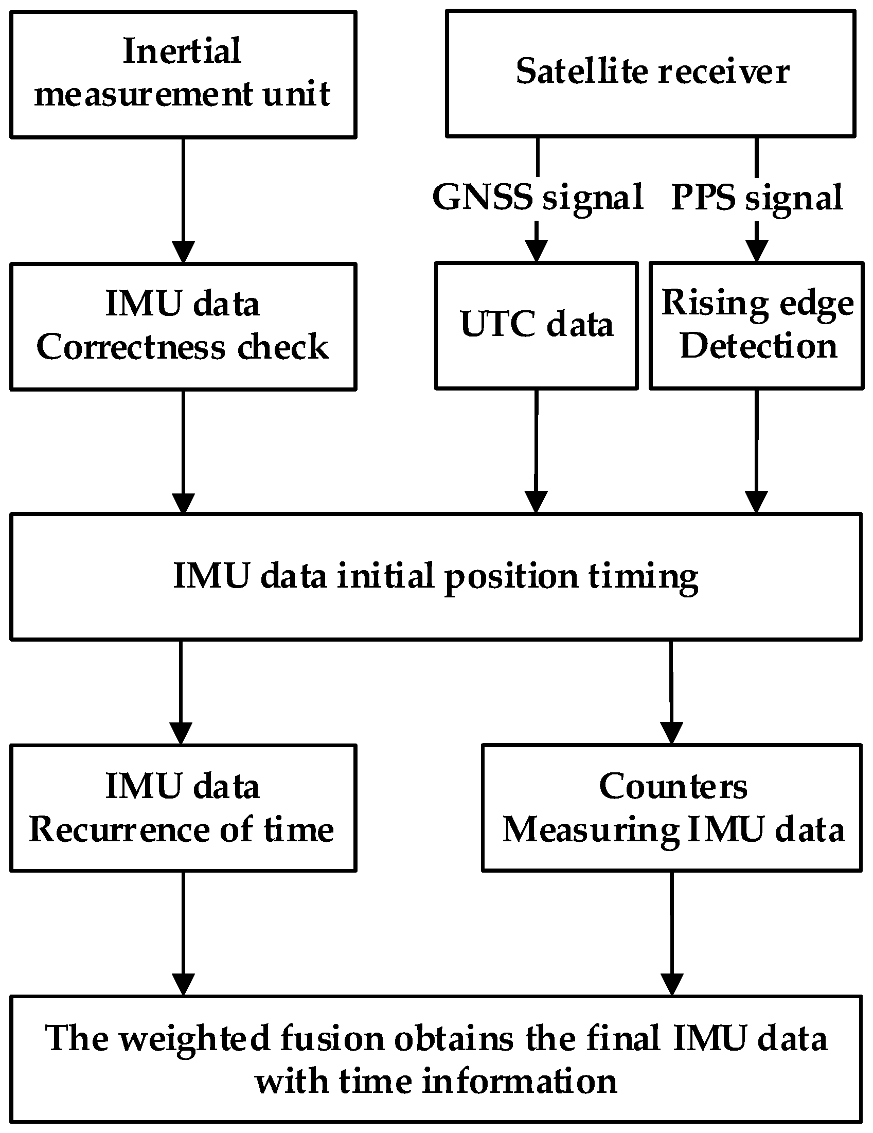
• Theoretical modeling: Based on the SINS/GNSS loosely coupled model, the 15-dimensional error state vector and the 6-dimensional observation vector are defined and the state equation and measurement equation are constructed.
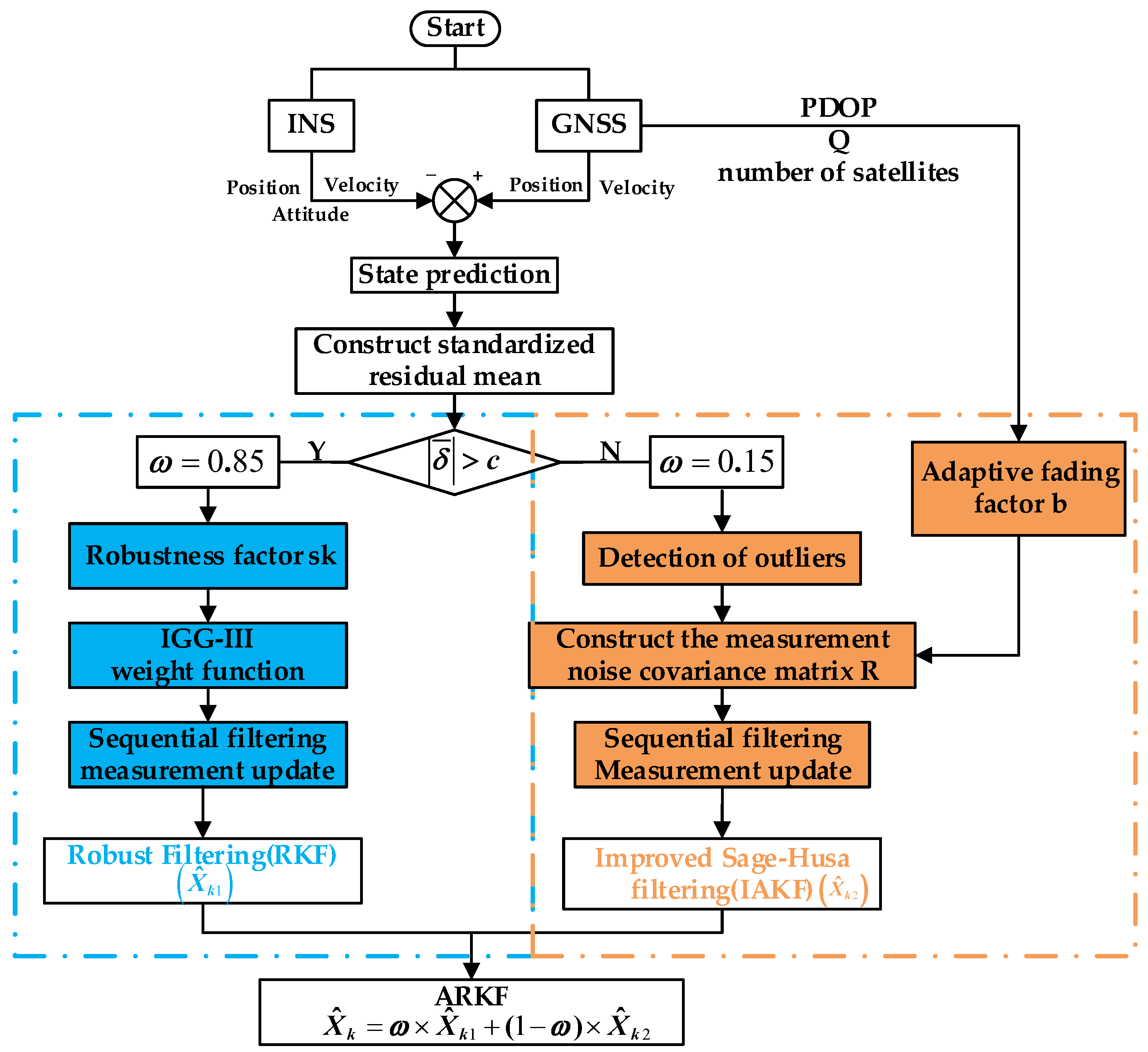
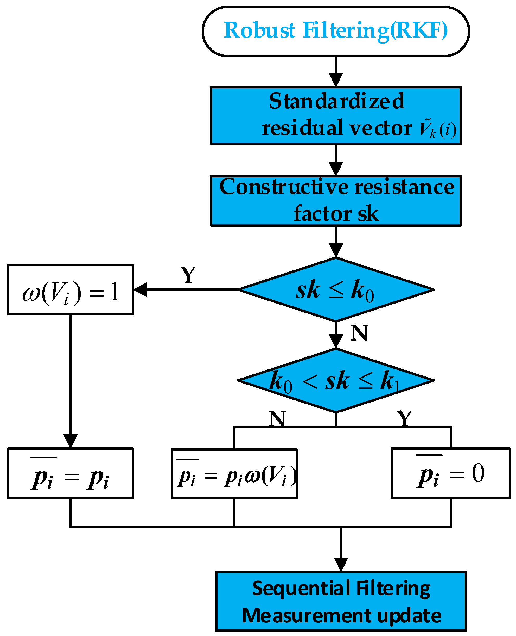
• Algorithm design: The dynamic fading factor is constructed by multi-source information fusion, and the sequential filtering is used to update the measurement to avoid the negative determination of the measurement noise covariance matrix. At the same time, the standardized residual and IGG-III weight function are combined to suppress the influence of abnormal observation on state update, and the two-factor robust mechanism is realized.
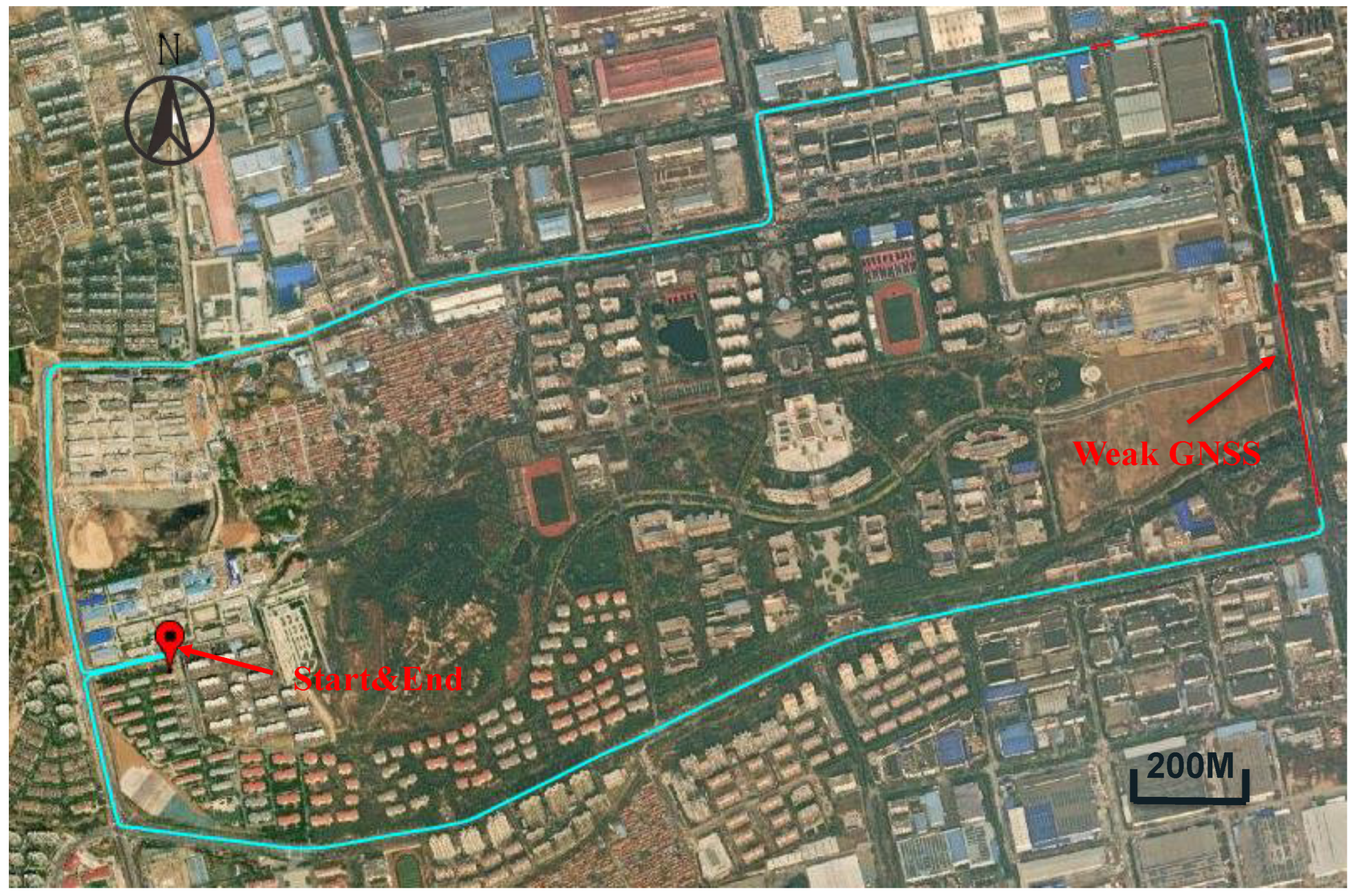
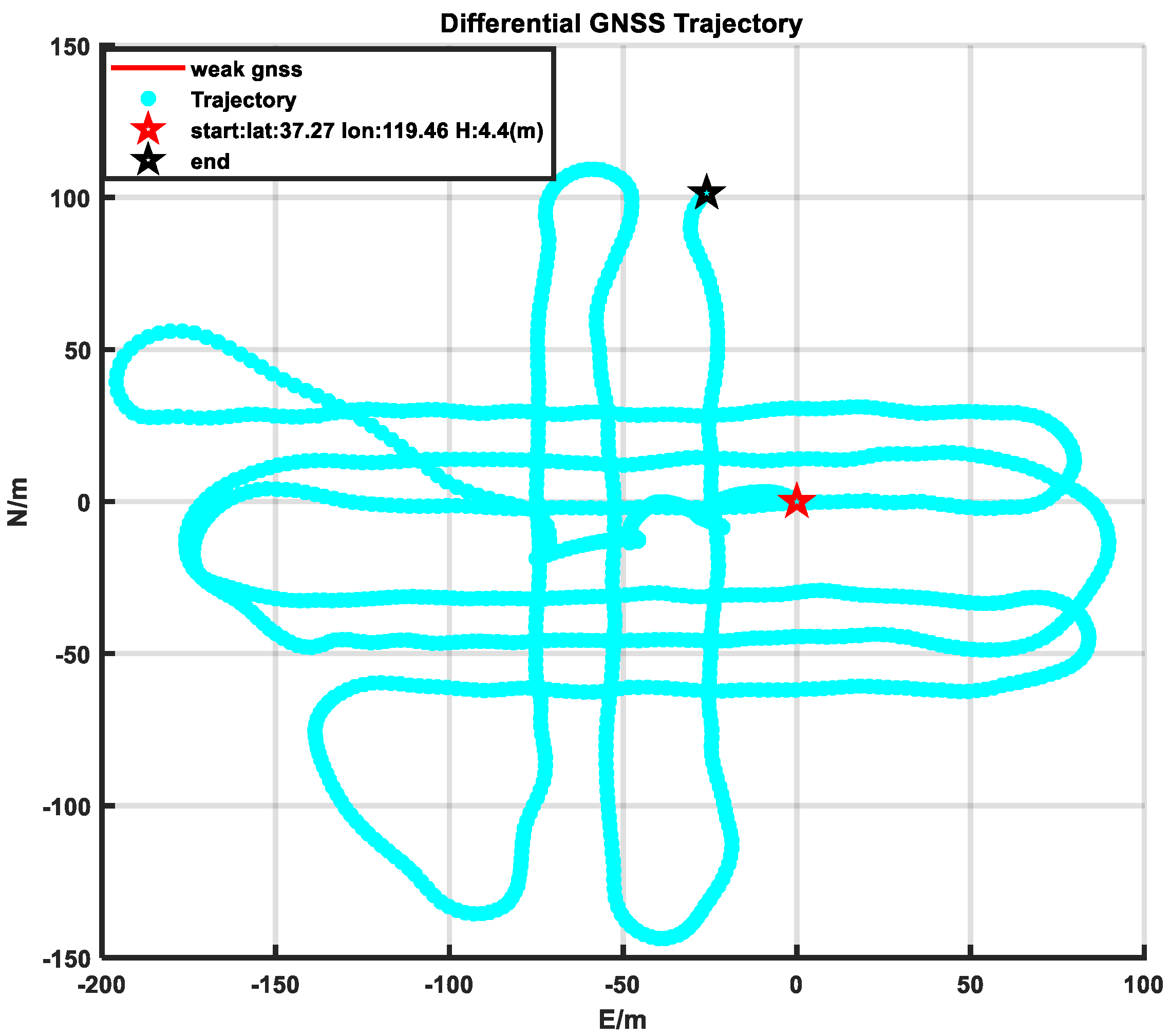
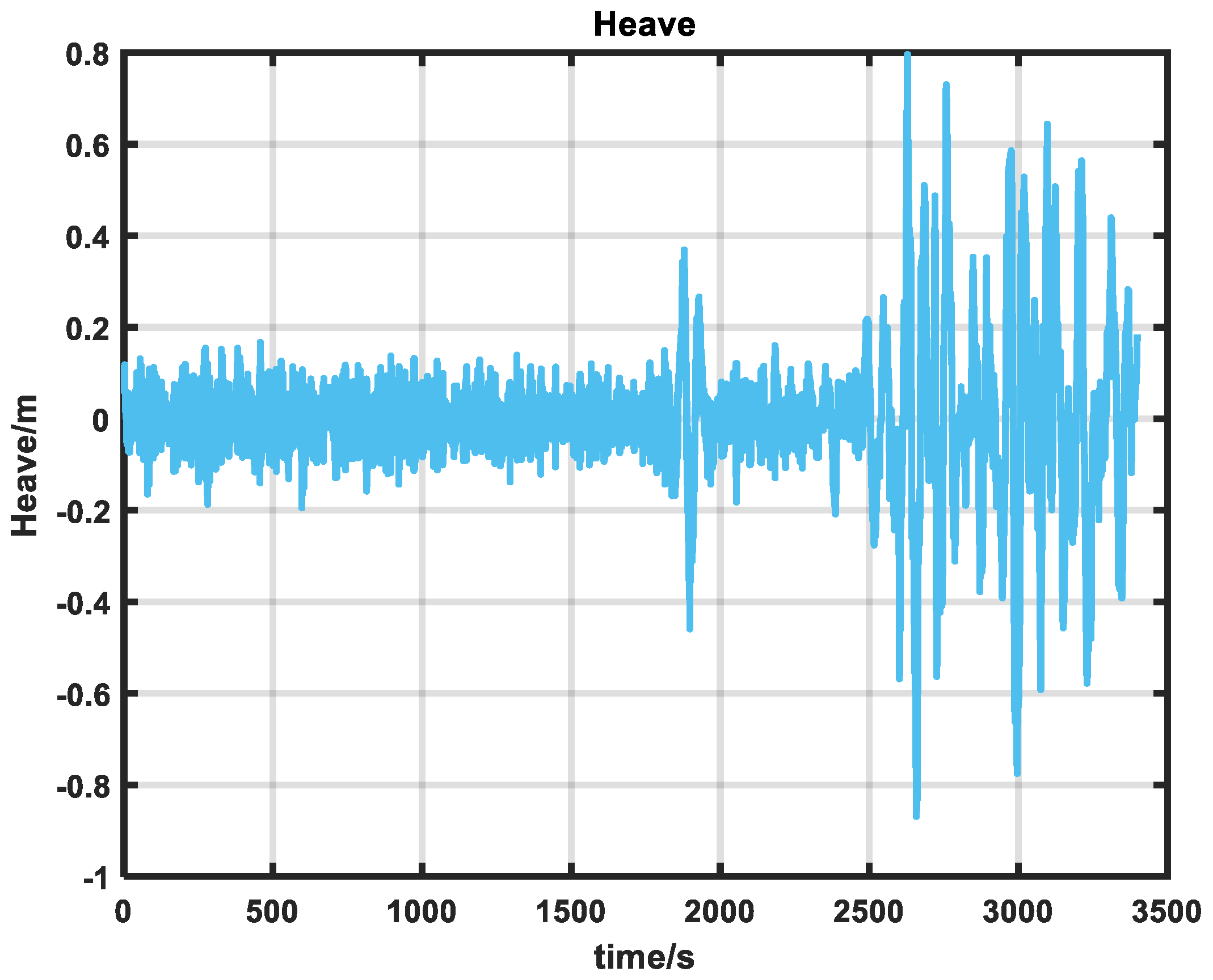
• Experimental verification: In order to verify the performance of the algorithm, a set of vehicle-mounted experiments was designed. The experimental time was about 20 min. Due to the high-rise occlusion, the data had a GNSS signal of about 200 s. A set of ship-borne experiments, three-level sea conditions, were designed, and the experiment lasted about 1 h. After the 2000s, the heave of the ship was significantly increased due to the wind and waves. The emergence of these abnormal conditions increases the uncertainty of navigation and can better verify the stability of the algorithm in a disturbed environment.

2.2. Combined SINS/GNSS Navigation Models

In this paper, based on the observation of position and velocity by GNSS, the GNSS/INS loose combination is studied to solve the nonlinear problem of the system [13]. The state space model and measurement model of SINS and GNSS integrated navigation system are as follows [14]:

$$\begin{array}{l}\left\{\begin{array}{c}{\mathit{X}}_{\mathit{k}}={\mathit{\Phi }}_{\mathit{k}/\mathit{k}-1}{\mathit{X}}_{\mathit{k}-1}+{\mathit{\Gamma }}_{\mathit{k}-1}{\mathit{W}}_{\mathit{k}-1}\\ {\mathit{Z}}_{\mathit{k}}={\mathit{H}}_{\mathit{k}}{\mathit{X}}_{\mathit{k}}+{\mathit{v}}_{\mathit{k}}\end{array}\right.\\ \left\{\begin{array}{l}\mathit{E}[{\mathit{W}}_{\mathit{k}}]=0,\hspace{1em}\mathit{E}[{\mathit{W}}_{\mathit{k}}{\mathit{W}}_{\mathit{j}}^{\mathrm{T}}]={\mathit{Q}}_{\mathit{k}}{\mathit{\delta }}_{\mathit{k}\mathit{j}},\hfill \\ \mathit{E}[{\mathit{V}}_{\mathit{k}}]=0,\hspace{1em}\mathit{E}[{\mathit{V}}_{\mathit{k}}{\mathit{V}}_{\mathit{j}}^{\mathrm{T}}]={\mathit{R}}_{\mathit{k}}{\mathit{\delta }}_{\mathit{k}\mathit{j}},\hfill \\ \mathit{E}[{\mathit{W}}_{\mathit{k}}{\mathit{V}}_{\mathit{j}}^{\mathrm{T}}]=0\hfill \end{array}\right.\end{array}$$

(1)

where ${\mathbf{\Phi }}_{\mathit{k}/\mathit{k}-1}$ is the state transfer matrix of the system; ${\mathbf{\Gamma }}_{\mathit{k}-1}$ is the noise driver matrix; ${\mathit{W}}_{k-1}$ is the process noise vector; ${\mathit{Q}}_k$ is the state noise covariance matrix; ${\mathit{R}}_k$ is the observation noise covariance matrix; meanwhile, ${\mathit{Q}}_k$, ${\mathit{R}}_k$ should be positive definite matrices; ${\mathit{X}}_{\mathit{k}}$ is the state vector; ${\mathit{Z}}_k$ denotes the measurement vector of the system output; ${\mathit{H}}_k$ is the measurement matrix; $v_k$ denotes the measurement noise, where the 21-dimensional state vector contains the navigation state error and the sensor error, defined as [15].

$${\mathit{X}}_{\mathit{k}}={\left[\begin{array}{ccccccc}\mathit{\delta }{\mathit{r}}^{\mathit{n}}& \mathit{\delta }{\mathit{v}}^{\mathit{n}}& \mathit{\varphi }& {\mathit{b}}_{\mathit{g}}& {\mathit{b}}_{\mathit{a}}& {\mathit{s}}_{\mathit{g}}& {\mathit{s}}_{\mathit{a}}\end{array}\right]}^{\mathrm{T}}$$

(2)

where $\mathit{\delta }{\mathit{r}}^{\mathit{n}}$ is the inertial position error vector; $\mathit{\delta }{\mathit{v}}^{\mathit{n}}$ is the inertial velocity error vector; $\mathit{\varphi }$ is the attitude error vector; ${\mathit{b}}_{\mathit{g}}$ is the three-axis gyroscope bias vector; ${\mathit{b}}_{\mathit{a}}$ is the three-axis accelerometer bias vector; ${\mathit{s}}_{\mathit{g}}$ is the gyroscope scale factor error; ${\mathit{s}}_{\mathit{a}}$ is the accelerometer scale factor error vector.

2.3. SINS/GNSS Adaptive Robust Filtering Algorithm Based on Improved Fading Factor (ARKF)

The SINS/GNSS adaptive robust filtering algorithm based on improved fading factor solves the problem that the traditional filtering algorithm is susceptible to non-Gaussian noise and abnormal observation in complex dynamic environment. The core of the algorithm is to dynamically adjust the filter by constructing a fading adaptive factor and a robust factor to improve the filtering performance and navigation accuracy.

The key to improving adaptive filtering is to construct a fading adaptive factor and adjust the measurement noise covariance matrix in real time, so as to enhance the adaptability of the filter to dynamic environmental changes. This paper comprehensively considers the four parameters of satellite geometric precision factor (PDOP value), solution quality factor (Q value), effective satellite observation number and observation vector residual, and dynamically adjusts the size of the adaptive factor. And the gross error detection is performed before the measurement update, and the upper and lower limits of the measurement variance are artificially set to avoid the influence of extreme values. When the PDOP value and Q value are low, and the number of effective satellite observations is sufficient, the measurement environment is better, the adaptive factor is close to 1, and the filter trusts the current observation data more. When the PDOP value and Q value are large, the number of effective satellite observations decreases or the observation residual increases, the adaptive fading factor decreases, and the filter reduces the weight of abnormal observations, thereby reducing the impact of abnormal data on state estimation. According to the evaluation results of the normalized vector residual mean, if a certain error standard C is met, the weight of the filter will be adjusted accordingly. Secondly, the robust factor is constructed, and the right function is used to determine the weight, so as to ensure the resistance of the robust filter to abnormal data. Finally, the fusion of these two filtering methods can further optimize the dynamic estimation accuracy of the system, especially in the case of complex environment or strong interference, to ensure the stable operation of the navigation system.

The flow chart of SINS/GNSS adaptive robust filtering algorithm based on improved fading factor is shown in Figure 1:

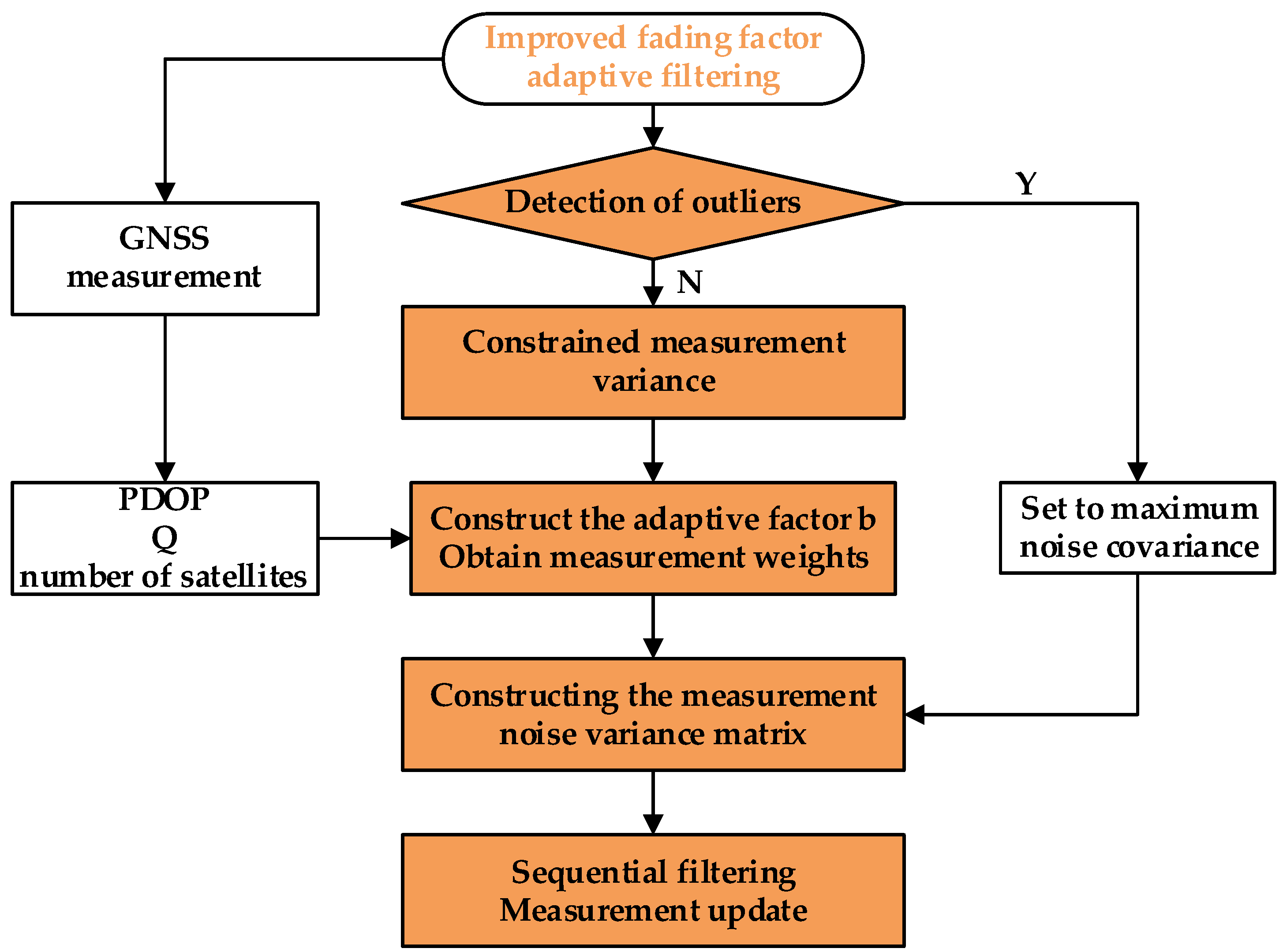
2.4. Improved Fading Factor Adaptive Filtering Algorithm (IAKF)

Since some information about the system model is implied in the measurement output, if the system model parameters are not accurate enough, some of the parameters can be modeled by adaptive estimation based on the measurement output [16,17].

When $\mathit{E}[{\mathit{W}}_{\mathit{k}}]$ and $\mathit{E}[{\mathit{V}}_{\mathit{k}}]$ do not satisfy equal to 0, using the traditional Kalman filter is prone to filter divergence and does not allow the system to reach the optimal estimation [18]. When the observation is in an abnormal state, the measurement noise will have a great impact on the filtering results. Therefore, the adaptive filtering is introduced to estimate the measurement noise while estimating the parameters. The system noise variance is difficult to adapt, and the measurement noise variance matrix is relatively easy to adapt. Therefore, the designed adaptive filter uses the output edge as the state estimation and the measurement noise identification. The adaptive filtering algorithm of the improved fading factor is as follows:

The measurement noise covariance matrix is adaptive by innovation. The measurement innovation is as follows [19]:

$${\hat{\mathit{V}}}_{\mathit{k}}={\mathit{Z}}_{\mathit{k}}-{\hat{\mathit{Z}}}_{\mathit{k}/\mathit{k}-\mathbf{1}}={\mathit{H}}_{\mathit{k}}{\mathit{X}}_{\mathit{k}}+{\mathit{V}}_{\mathit{k}}-{\mathit{H}}_{\mathit{k}}{\hat{\mathit{X}}}_{\mathit{k}/\mathit{k}-\mathbf{1}}={\mathit{H}}_{\mathit{k}}{\tilde{\mathit{X}}}_{\mathit{k}/\mathit{k}-\mathbf{1}}+{\mathit{V}}_{\mathit{k}}$$

(3)

where ${\hat{\mathit{V}}}_{\mathit{k}}$ is the measurement innovation; ${\mathit{Z}}_{\mathit{k}}$ denotes the observation vector; ${\hat{\mathit{X}}}_{\mathit{k}/\mathit{k}-1}$ denotes the predicted state vector; ${\mathit{H}}_{\mathit{k}}$ is a measurement matrix [20,21]:

$${\hat{\mathit{V}}}_{\mathit{k}}~\mathrm{N}(0,{\mathit{H}}_{\mathit{k}}{\mathit{P}}_{\mathit{k}/\mathit{k}-1}{\mathit{H}}_{\mathit{k}}^{\mathrm{T}}+{\mathit{R}}_{\mathit{k}})$$

(4)

${\mathit{R}}_{\mathit{k}}$ is the measurement noise covariance matrix. where the measurement innovation is considered to be white noise with 0 as the mean and ${\mathit{H}}_{\mathit{k}}{\mathit{P}}_{\mathit{k}/\mathit{k}-\mathbf{1}}{\mathit{H}}_{\mathit{k}}^{\mathrm{T}}+{\mathit{R}}_{\mathit{k}}$ represents the variance when the system is working normally [22]; and ${\mathit{P}}_{\mathit{k}/\mathit{k}-\mathbf{1}}$ is the covariance matrix of the prediction error. The measurement noise variance matrix is estimated as follows [23]:

$${\hat{\mathit{R}}}_{\mathit{k}}={\displaystyle \frac{1}{k}}\sum _{i=1}^k({\tilde{\mathit{V}}}_{\mathit{i}/\mathit{i}-\mathbf{1}}{\tilde{\mathit{V}}}_{\mathit{i}/\mathit{i}-\mathbf{1}}^{\mathrm{T}}-{\mathit{H}}_i{\mathit{P}}_{\mathit{i}/\mathit{i}-1}{\mathit{H}}_{\mathit{i}}^T)$$

(5)

$${\hat{\mathit{R}}}_{\mathit{k}}={\displaystyle \frac{1}{k}}[\sum _{i=1}^{k-1}({\tilde{\mathit{V}}}_{\mathit{i}/\mathit{i}-\mathbf{1}}{\tilde{\mathit{V}}}_{\mathit{i}/\mathit{i}-\mathbf{1}}^{\mathrm{T}}-{\mathit{H}}_{\mathit{i}}{\mathit{P}}_{\mathit{i}/\mathit{i}-\mathbf{1}}{\mathit{H}}_{\mathit{i}}^{\mathrm{T}})+({\tilde{\mathit{V}}}_{\mathit{k}/\mathit{k}-\mathbf{1}}{\tilde{\mathit{V}}}_{\mathit{k}/\mathit{k}-\mathbf{1}}^{\mathrm{T}}-{\mathit{H}}_{\mathit{k}}{\mathit{P}}_{\mathit{k}/\mathit{k}-\mathbf{1}}{\mathit{H}}_{\mathit{k}}^{\mathrm{T}})]$$

(6)

$$\hat{\mathit{R}}=(1-{\beta }_k){\hat{\mathit{R}}}_{\mathit{k}-\mathbf{1}}+{\beta }_k({\tilde{\mathit{V}}}_{\mathit{k}/\mathit{k}-\mathbf{1}}{\tilde{\mathit{V}}}_{\mathit{k}/\mathit{k}-\mathbf{1}}^{\mathrm{T}}-{\mathit{H}}_{\mathit{k}}{\mathit{P}}_{\mathit{k}/\mathit{k}-\mathbf{1}}{\mathit{H}}_{\mathit{k}}^{\mathrm{T}})$$

(7)

In Equation (7):

$${\beta }_k={\displaystyle \frac{{\beta }_{k-1}}{{\beta }_{k-1}+b}}$$

(8)

where ${\beta }_0=1,{\beta }_{\infty }=1-b$, b is called the adaptive fading factor $(0<b<1)$.

In Equation (5), when the actual noise is relatively small, it is easy to have negative determination of the measurement variance, which is handled here by using sequential filtering.

$${\rho }_k^{(i)}={({\tilde{V}}_{k/k-1}^{(i)})}^2-H_k^{(i)}{P}_{k/k-1}^{(i)}{(H_k^{(i)})}^{\mathrm{T}}$$

(9)

In order to prevent the filter from becoming unstable due to inaccurate measurement noise estimation. By limiting the update range of the estimated measurement noise variance, the stability of the filter is improved. The upper and lower limits of $R_k^{(i)}$ are set artificially. In the experiment, the lower limit $R_{min}$ is 0.3 times the nominal variance of GNSS position noise and velocity noise, and the upper limit $R_{max}$ is 3 times the nominal variance of GNSS position noise and velocity noise. This setting can prevent extreme values from causing filter divergence, while retaining the space for dynamic adjustment of noise [24]. There are as follows:

$${\hat{R}}_k^{(i)}=\left\{\begin{array}{ll}\hspace{1em}\hspace{1em}{R}_{\min }^{(i)}\hfill & {\rho }_k^{(i)}\le R_{\min }^{(i)}\hfill \\ (1-{\beta }_k){\hat{R}}_{k-1}^{(i)}+{\beta }_k{\rho }_k^{(i)}\hfill & R_{\min }^{(i)}<{\rho }_k^{(i)}<R_{\max }^{(i)}\hfill \\ \hspace{1em}\hspace{1em}{R}_{\max }^{(i)}\hfill & {\rho }_k^{(i)}\ge R_{\max }^{(i)}\hfill \end{array}\right.$$

(10)

In this paper, we also add fault judgment on the basis of adaptive filtering, according to Equation (10) when the system is fault-free ${\tilde{\mathit{V}}}_{\mathit{k}/\mathit{k}-\mathbf{1}}\sim \mathit{N}(0,{\mathit{H}}_{\mathit{k}}{\mathit{P}}_{\mathit{k}/\mathit{k}-\mathbf{1}}{\mathit{H}}_{\mathit{k}}^{\mathrm{T}}+{\mathit{R}}_{\mathit{k}})$, based on the residual detection technique, the filtering dispersion judgment is based on the following [25]:

$${\tilde{\mathit{V}}}_{\mathit{k}/\mathit{k}-\mathbf{1}}^{\mathrm{T}}{\tilde{\mathit{V}}}_{\mathit{k}/\mathit{k}-\mathbf{1}}>3tr({\mathit{H}}_{\mathit{k}}{\mathit{P}}_{\mathit{k}/\mathit{k}-\mathbf{1}}{\mathit{H}}_{\mathit{k}}^{\mathrm{T}}+{\mathit{R}}_{\mathit{k}})$$

(11)

If the above equation is valid, it means that the actual error value is more than 3 times that of the theoretical value, according to the principle that it is anomalous value, and the use of these data for filtering can easily lead to unstable filtering dispersion, at this time, let ${\hat{R}}_k^{(i)}=R_{\max }^i$, through the increase in the large number of measurement of the noise variance array to make the anomalous value of the filtering system weighting is reduced to reduce the impact on the results.

In order to obtain the adaptive fading factor b, the adaptive fading factor is constructed by the PDOP value, Q value, effective satellite observation number and measurement vector residual obtained by satellite observation. Firstly, the measurement scale factors $\alpha$, $\beta$ and $\lambda$ are obtained to adjust the sensitivity of the system to the measurement error. The system can evaluate the quality of the current environment and observation data in real time and dynamically adjust the weight of the filter. The following is the formula:

$$\left\{\begin{array}{l}\alpha ={\displaystyle \frac{PDOP-PDO{P}_{\min }}{PDO{P}_{\max }-PDO{P}_{\min }}}\\ \beta ={\displaystyle \frac{Q-Q_{\min }}{Q_{\max }-Q_{\min }}}\\ \lambda =1-{\displaystyle \frac{satnum-satnu{m}_{\min }}{satnu{m}_{\max }-satnu{m}_{\min }}}\end{array}\right.$$

(12)

In this formula, the factor $\alpha$ is used to adjust the influence of PDOP. PDOP represents the geometric distribution of the satellite. The lower PDOP indicates a better satellite geometric distribution and usually has better positioning accuracy, while the higher PDOP indicates a worse geometric distribution. When PDOP is poor, this factor is at a lower value, which makes the filtering system weaken the influence of measurement innovation on positioning, thus improving the reliability of the filtering. The Q value measures the quality of the satellite positioning solution and represents the accuracy and reliability of the GNSS positioning data. The $\beta$ factor ensures that when Q is high, it usually indicates that the quality of the positioning solution is poor. At this time, the filter is dynamically adjusted to reduce the dependence on the data. The $\lambda$ factor is adjusted according to the number of effective satellites used for positioning. When the number of satellites is large, it means that the number of satellites involved in the solution is large, and the positioning is usually more accurate. The $\lambda$ factor helps the system to adapt to changes in the number of visible satellites. When the number of satellites is small, it can still maintain stability.

The construction formula for the fading adaptive factor is as follows:

$$\left\{\begin{array}{l}\mathrm{u}={\displaystyle \frac{{\tilde{\mathit{V}}}_{\mathrm{k}}^{\mathrm{T}}{\tilde{\mathit{V}}}_{\mathrm{k}}}{3\times \left|\mathrm{t}\mathrm{r}(\mathit{H}\mathit{P}{\mathit{H}}^T+\mathit{R})\right|}}\\ {\omega }_1+{\omega }_2+{\omega }_3=1\\ \mathrm{b}=(1-\mathrm{u})\times [0.999-({\omega }_1\times \alpha +{\omega }_2\times \beta +{\omega }_3\times \lambda )\ast \mathrm{A}]\end{array}\right.$$

(13)

where b is the adaptive fading factor, the measurement noise weight is adjusted by the adaptive fading factor. The parameter u becomes larger, so that the adaptive fading factor b decreases, and by reducing the value of b, the system’s response to the measurement noise can be accelerated, so as to improve the tracking accuracy, especially in the case of large noise fluctuations, so that it can be better adjusted and adapted to the current environmental changes.

A represents the amplitude of the amplitude adjustment coefficient of the adaptive fading factor, and the value is 0.07. Its core significance is to balance the dynamic response speed of the noise estimation, so that the value of the fading factor is kept in the range of [0.9–0.999] as much as possible [26]. If the fading factor is too small, the noise estimation result will jump too violently.

For the selection of the adaptive fading factor amplitude adjustment coefficient A, we re-compare the performance of the adaptive fading factor when A = 0.05, A = 0.07, and A = 0.09. It can be seen from the Figure 2 that when A = 0.05, the adaptive fading factor b is insensitive to changes in the disturbance environment, which weakens the system’s adaptive ability and reduces the response speed. When A = 0.09, the known adaptive fading factor b should be between [0.9–0.999]. When b is too small, it is easy to cause instability of the system. Therefore, when A = 0.07, the response speed and stability of the filter achieve the best balance.

It is the weight coefficient of the satellite geometric accuracy factor PDOP, the weight coefficient of the solution factor Q, and the weight coefficient of the number of effective satellite observations. The selection and distribution of weight coefficients adhere to the principle of significant influence of geometric accuracy factor, satellite solution factor and effective satellite observation number on satellite positioning error.

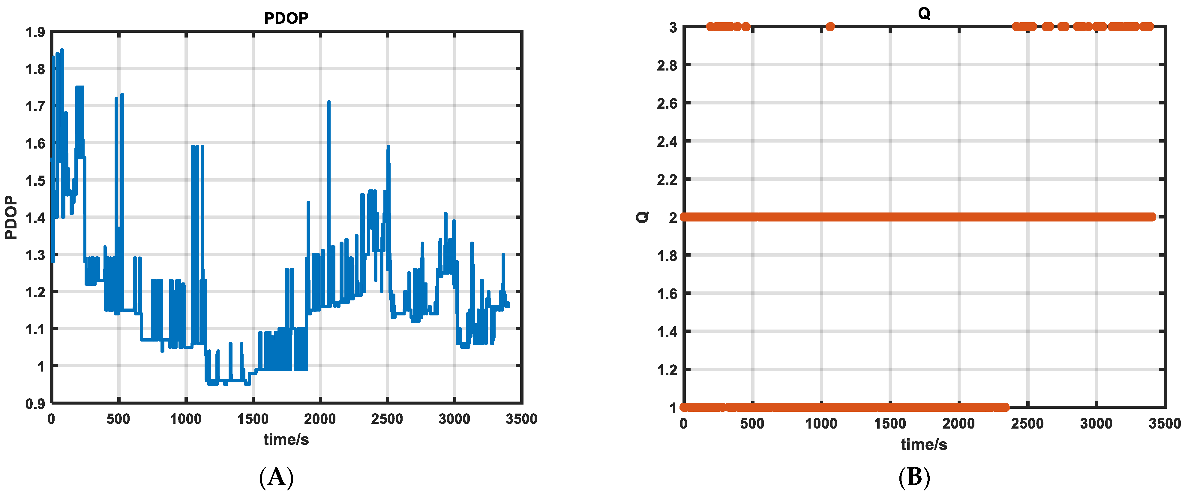
• Satellite geometric precision factor (PDOP): it directly reflects the influence of satellite geometric distribution on positioning accuracy [27], and its weight ${\omega }_1$ is set to 0.4.
• Satellite solution factor (Q): used to quantify the quality of GNSS solution.

  Table 1. Solution quality factor.

  Q	Description	3D Accuracy (m)
  1	Fixed integer	0.00–015
  2	Converged float or noisy fixed integer	0.05–0.40
  3	Converging float	0.20–1.00
  4	Converging float	0.50–2.00
  5	DGPS	1.00–5.00

  shows the relationship between Q value and 3D positioning accuracy. The Q value directly reflects the error range of GNSS positioning. Its weight ${\omega }_2$ is also set to 0.4.
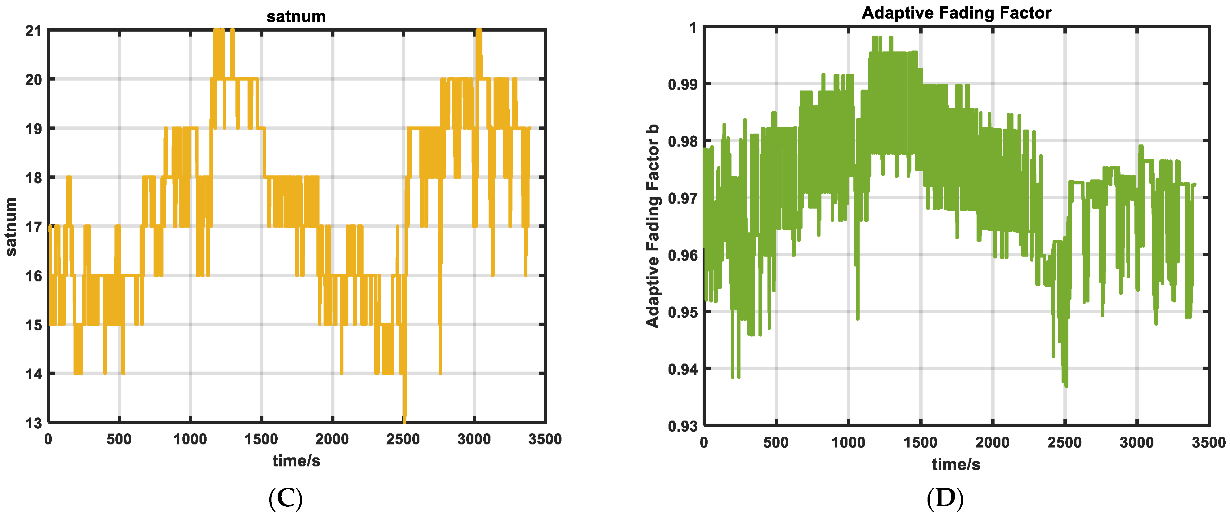
• The number of effective satellite observations (Satnum): The number of effective satellite observations does not directly reflect the advantages and disadvantages of GNSS positioning solutions, but it can reflect the redundancy of GNSS positioning. Therefore, this paper sets its weight ${\omega }_3$ to 0.2.

In the filtering process, when the GNSS observation results are abnormal, the PDOP and Q values will increase significantly, which represents the deterioration of the geometric distribution of the satellite and the decrease in the solution quality [28]. This change means that the system faces greater uncertainty, which may lead to a decrease in the confidence of the filter in the observed data. At the same time, the observation residuals of GNSS will also increase, and the system will increase the adaptability to the measurement noise according to the change in these abnormal residuals, and it will gradually improve the response ability to the noise estimation. In addition, the parameter u will also increase, thus prompting the adaptive fading factor b to decrease within a reasonable range. The dynamic adjustment of the fading factor b enables the filtering system to flexibly adjust the measurement noise covariance matrix according to the actual observation conditions, thereby improving the robustness of the system in the face of complex disturbances. It effectively suppresses the influence of abnormal data on the filtering results and prevents abnormal observations from adversely affecting the navigation system.

The value of fading factor b should not be too small. If b is set too small, the response of the system to noise estimation will change dramatically. This change may lead to unstable noise estimation results and jump phenomenon, thus affecting the stability and positioning accuracy of the filter. Therefore, the fading factor should be kept within a reasonable range, usually set between $[0.9,0.999]$ to ensure that the filtering system can respond smoothly during dynamic adjustment [29,30].

• When the GNSS observations are reliable, when the satellite geometry is well distributed and the number of effective satellite observations is sufficient, the PDOP value and Q value are usually low, and the system can obtain high-quality positioning results [31]. In this case, the fading factor b will increase, the confidence of the filter to the observation data will increase, and the system believes that the measurement data are more reliable. The update of the measurement noise covariance matrix will become more stable, and the filter will give greater weight when processing the observation data, so that the estimation results are more dependent on the observation data.
• When the GNSS observations are unreliable, when the satellite geometric distribution is poor and the number of effective satellite observations is insufficient, the PDOP value and Q value will increase, and the system will face higher uncertainty and positioning error. In this case, the quality of the observation data is poor, and there may be a large measurement error or noise, which will lead to a decrease in the trust of the filter to the observation data [31]. As the fading factor decreases, the update of the measurement noise covariance matrix becomes more conservative, the trust of the filter to the measurement data decreases, and the system depends more on the inertial navigation system (SINS). This dynamic adjustment can effectively avoid the estimation error caused by measurement noise or abnormal data.

Therefore, the dynamic adjustment mechanism of the adaptive fading factor designed in this paper can make the system flexibly adapt to the changes under different environmental conditions. Under harsh environmental conditions, a large number of measurement noise matrices are obtained by reducing the b value, and the sensitivity to measurement noise is enhanced. When the observation conditions are improved, the fading factor approaches 1, which helps the system to make more accurate use of historical data, so as to maintain efficient noise suppression and positioning accuracy during long-term operation. In the filtering system, with the dynamic adjustment of the fading factor, the system can quickly reduce the dependence on abnormal observations in harsh environments, and restore a high degree of trust in valid data when the observation conditions are good. Through this adaptive mechanism, the system can automatically adjust the trust degree of different measurements according to the real-time observation quality and achieve higher positioning accuracy and robustness. Especially in the environment of GNSS signal occlusion or large external vibration, it can effectively avoid the attenuation of filter performance and the expansion of positioning error.

In summary, the overall flow chart of the improved adaptive filtering algorithm is shown in Figure 3:

2.5. Robust Filtering (RKF)

Robust filtering can solve the problem of outliers and errors in navigation systems. By reducing the influence of outliers on the filtering results, robust filtering can avoid filtering divergence and ensure the stable operation of the integrated navigation system in various complex environments [32]. The robust filtering process is as follows:

The prediction residual vector can better respond to the anomalies of state perturbations [33]. Then, the weight function is constructed based on the standardized residual vector. The construction process of standardized vector residual construction and anti-differential factor $sk$ is as follows:

$${\delta }_k={\displaystyle \frac{|{\tilde{\mathit{V}}}_{\mathit{k}}(i)|}{\sqrt{{\mathit{R}}_{\mathit{k}}[i,i]}}}$$

(14)

Sorting ${\delta }_k$, we have ${\delta }_k^{\mathrm{sorted}}[j]\ge {\delta }_k^{\mathrm{sorted}}[j+1],\hspace{1em}\forall j\in [0,n-2]$. Since the observation vector is 6-dimensional, $n=6$, is taken:

$${\delta }_k^{mid}={\displaystyle \frac{{\delta }_k^{\mathrm{sorted}}[3]+{\delta }_k^{\mathrm{sorted}}[4]}{2}}$$

(15)

The vector of resistance factor is as follows:

$$sk={\displaystyle \frac{|{\tilde{\mathit{V}}}_{\mathit{k}}(i)|}{{\delta }_k^{mid}\sqrt{{\mathit{R}}_{\mathit{k}}[i,i]}}}$$

(16)

Here, we use a three-stage weight reduction factor, IGGIII weight function [27,33]:

$$\overline{p_i}=\left\{\begin{array}{ll}{p}_i\hfill & sk\le k_0\hfill \\ p_i\omega (\widetilde{V_i})\hfill & k_0<sk\le k_1\hfill \\ 0\hfill & sk>k_1\hfill \end{array}\right.=\left\{\begin{array}{ll}{p}_i\hfill & sk\le k_0\hfill \\ p_i{\displaystyle \frac{k_0}{\left|\widetilde{V_i}\right|}}{\left({\displaystyle \frac{k_1-\left|\widetilde{V_i}\right|}{k_1-k_0}}\right)}^2\hfill & k_0<sk\le k_1\hfill \\ 0\hfill & sk>k_1\hfill \end{array}\right.$$

(17)

where $\left|\widetilde{V_i}\right|$ denotes the standardized residual; $k_0$ and $k_1$ are constants, usually chosen as $k_0=1.0~1.5$, $k_1=2.5~8.0$.

Sequential filtering is used to update measurements. In the robust filtering framework, only the data at the current time and the estimation results at the previous time are needed, and the weight can be dynamically adjusted according to the weighting factor and residual of the current observation without storing all the historical data [34].

$$\left\{\begin{array}{l}{\mathit{K}}_k^{(N)}=\overline{p_i}{\mathit{p}}_k^{(N-1)}{({\mathit{H}}_k^{(N)})}^T{[{\mathit{H}}_k^{(N)}{\mathit{p}}_k^{(N-1)}{({\mathit{H}}_k^{(N)})}^T+R_k^{(N)}]}^{-1}\\ {\mathit{X}}_k^{(N)}={\mathit{X}}_k^{(N-1)}+{\mathit{K}}_k^{(N)}({\mathit{Z}}_k^{(N)}-{\mathit{H}}_k^{(N)}{\mathit{X}}_k^{N-1})\\ {\mathit{p}}_k^{(N)}=(\mathit{I}-{\mathit{K}}_k^{(N)}{\mathit{H}}_k^{(N)}){\mathit{p}}_k^{(N-1)}{(\mathit{I}-{\mathit{K}}_k^{(N)}{\mathit{H}}_k^{(N)})}^T+{\mathit{K}}_k^{(N)}{\mathit{R}}_k^{(N)}{\mathit{K}}_k^{(N)T}\end{array}\right.$$

(18)

In summary, the overall flow chart of the robust filtering algorithm is as follows: In summary, the overall flow chart of the robust filtering algorithm is shown in Figure 4:

2.6. Data Collection and Processing Analysis Strategy

The inertial navigation of SINS/GNSS integrated navigation vehicle data adopts Honeywell HG4930, and its sampling frequency is 100 Hz. GNSS uses a single antenna with a sampling frequency of 5 Hz. The vehicle line is a circle around Shandong University of Science and Technology. The experiment lasted about 20 min. The ship-borne data also uses HG4930 with a frequency of 100 Hz, and the GNSS sampling frequency is 10 Hz. The ship-borne route revolves around the offshore wind farm in Changyi, and the experiment time is about 1 h. The time synchronization of GNSS and SINS is shown in Figure 5. According to the satellite data, the UTC and PPS signals are obtained. The initial data of IMU is timed by PPS, and the subsequent data are recursively timed according to the initial time of IMU, and the subsequent data are measured by timer. The final IMU data with time information is obtained by weighted fusion of recursive time and measurement time [35].

3. Experimental Demonstration and Analysis of Results

3.1. Experimental Environment

In order to evaluate the performance of the SINS/GNSS adaptive robust filtering algorithm based on the improved fading factor, a set of vehicle-mounted measured data collected in the complex environment of Qingdao City in 2024 was processed and analyzed (Figure 6a); a set of ship-borne measured data collected in the sea area near Changyi, Weifang, in 2024 under heave, low frequency, and high vibration environment are analyzed (Figure 6b).

The INS data of the following two sets of experiments were collected by HG4930, and the performance index parameters are shown in

Table 2. HG4930 performance parameters.

	Performance Parameters	HG4930
gyros	$\mathrm{R}\mathrm{a}\mathrm{n}\mathrm{g}\mathrm{e}/(\mathrm{deg}/\mathrm{s})$	±400
	$\mathrm{B}\mathrm{i}\mathrm{a}\mathrm{s} \mathrm{i}\mathrm{n}\mathrm{s}\mathrm{t}\mathrm{a}\mathrm{b}\mathrm{i}\mathrm{l}\mathrm{i}\mathrm{t}\mathrm{y}/(\mathrm{deg}/\mathrm{h})$	0.35
	$\mathrm{A}\mathrm{R}\mathrm{W}/(\mathrm{deg}/\sqrt{\mathrm{h}})$	0.05
accelerometer	$\mathrm{R}\mathrm{a}\mathrm{n}\mathrm{g}\mathrm{e}/\mathrm{g}$	±20
	$\mathrm{B}\mathrm{i}\mathrm{a}\mathrm{s} \mathrm{i}\mathrm{n}\mathrm{s}\mathrm{t}\mathrm{a}\mathrm{b}\mathrm{i}\mathrm{l}\mathrm{i}\mathrm{t}\mathrm{y}/\mathrm{m}\mathrm{g}$	0.05
	$\mathrm{V}\mathrm{R}\mathrm{W}/(\mathrm{m}/\mathrm{s}/\sqrt{\mathrm{h}})$	0.05

.

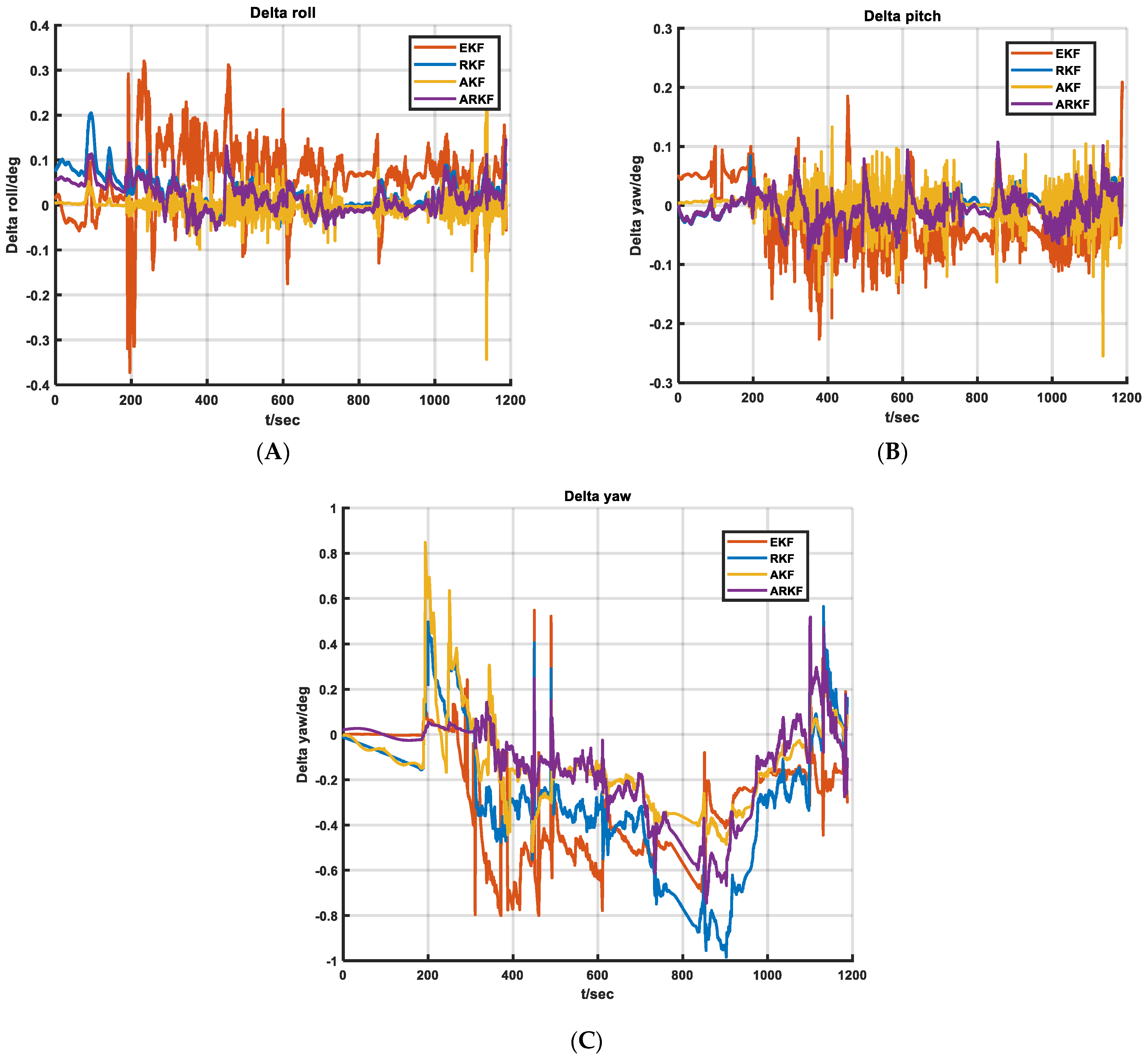
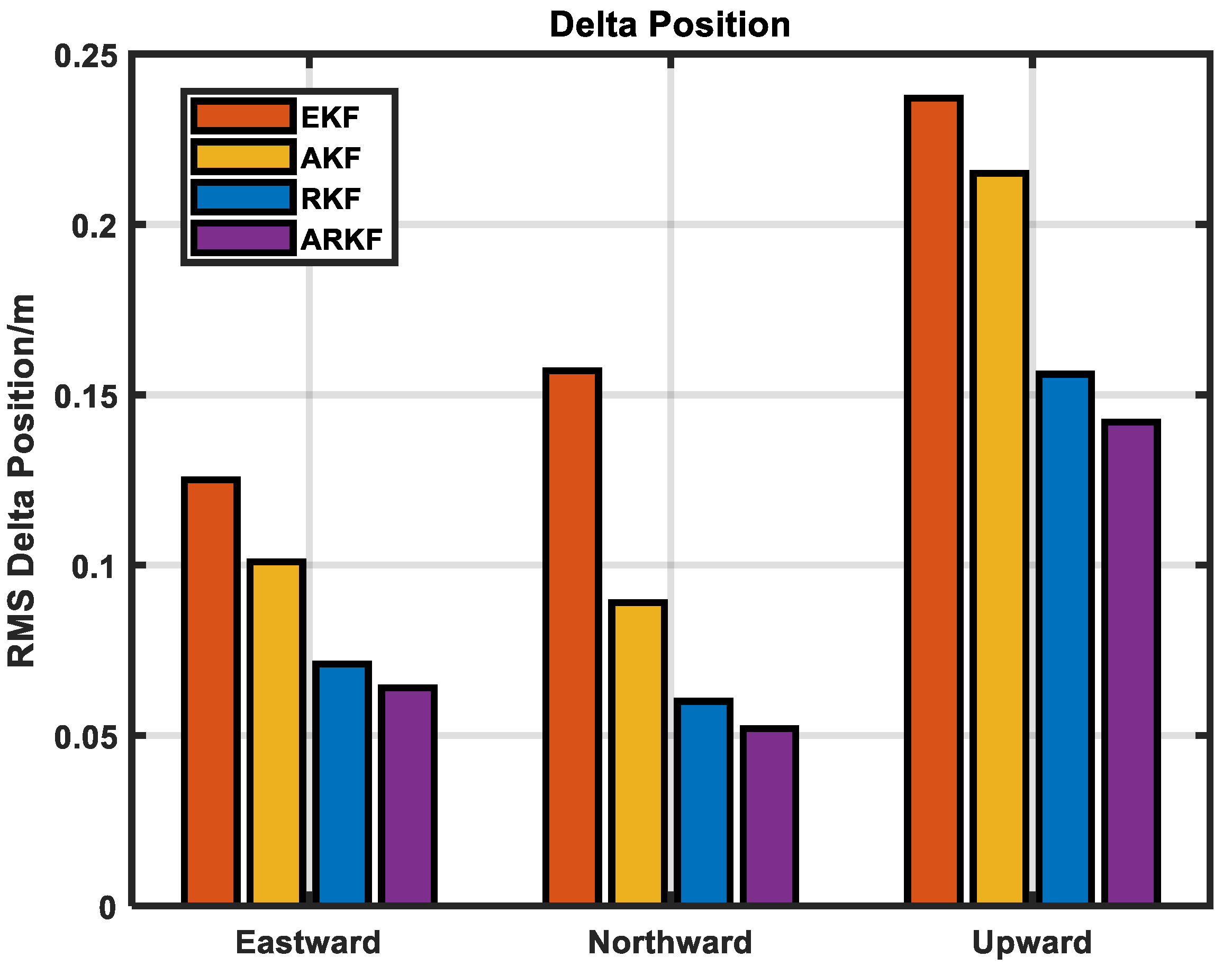
3.2. In-Vehicle Experiments

GNSS uses the differential positioning solution, and the GNSS base station is set up in the comprehensive building of Shandong University of Science and Technology Science Park, with a baseline length of about 1 km. The experiment lasted for about 1200 s. The experimental scene was selected as a complex urban environment, and the sports car experiment was carried out around Shandong University of Science and Technology.

The GNSS differential sports car trajectory is as follows Figure 7 shows that the differential signal is lost during the experiment. The satellite signal will be interfered or reflected due to the occlusion of the building; similarly, satellite signals may also be reflected by surrounding buildings or objects, resulting in multipath effects. The signal incorrectly receives the reflected wave, affecting the accuracy of positioning [36].

Four different schemes are designed for this data set: method one uses extended Kalman filter (EKF); the second method is the Sage-Husa adaptive Kalman filter (AKF); the third method is robust filtering (RKF); method 4 uses the filtering method (ARKF) mentioned in this paper. The high-precision navigation results obtained by NovAtel’s post-processing software Inertial Explorer 8.70 are used as the true value of the reference ground [37].

Figure 8A shows the geometric accuracy factor of the vehicle-borne experimental satellite, which directly reflects the influence of the distribution of the satellite geometry on the positioning error. When the vehicle passes under the tall buildings between 600 s and 800 s, most of the satellite signals are blocked, resulting in poor satellite geometry, which affects the observation effect of differential positioning. Figure 8B represents the satellite solution factor (Q), which is used to quantify the GNSS solution quality. The Q value can directly reflect the problem of satellite positioning difference between 600 and 800 s. Figure 8C shows the number of satellites involved in the solution in the vehicle experiment. There are only four satellites involved in the solution between 600 and 800 s, and the solution quality is poor. Figure 8D shows the change in adaptive fading factor b in the vehicle experiment. In the case of poor satellite solution quality, the filtering system can quickly adapt to environmental changes by adjusting the adaptive fading factor to obtain the optimal measurement noise matrix in the current situation. When the observation conditions are good and the measurement data are reliable, the value of the adaptive fading factor approaches 1, so that the measurement noise is closer to the historical value. This adjustment helps to improve the smoothness and stability of measurement noise, effectively reduce the impact of noise fluctuations on system performance, and ensure the stability of positioning accuracy.

The position, velocity, and attitude errors obtained by using the above four methods and professional solution software are shown in Figure 9 and Figure 10.

Figure 9A,C,E represent the comparison of the position errors of the four algorithms in the northeast direction. Figure 9B,D,F represent the comparison of the velocity errors of the four algorithms in the northeast direction, respectively. In the 600–800 s period with poor satellite observation conditions, the algorithm proposed in this paper shows more stable error characteristics than the other three algorithms. Specifically, the error value approaches 0, indicating that the algorithm can effectively deal with the unfavorable observation environment and reduce the influence of external factors on the positioning accuracy.

Figure 10A–C represent the error changes in the four algorithms in the roll, pitch, and heading directions with time. According to the figure, because the algorithm in this paper has adaptive characteristics, it can be adjusted according to different environmental conditions. The proposed algorithm (ARKF) shows good stability and smoothness in the estimation of roll, pitch, and heading angles.

In summary, EKF shows large transient fluctuations in multiple images, especially in areas with high GNSS occlusion. This shows that EKF has poor response to nonlinear and dynamic complex systems. The algorithm in this paper can quickly track the system state in areas with large dynamic changes, and there is no significant deviation or oscillation. The algorithm in this paper has high tracking accuracy for changes and can quickly recover to a stable state. In summary, the algorithm in this paper shows obvious smoothness and has the smallest fluctuation compared with other algorithms. In order to further compare the accuracy of the position, velocity, and attitude of the four schemes, the position and velocity error (RMS) are plotted as a histogram (Figure 11), and the corresponding results are also summarized in

Table 3. Vehicle-mounted experiments. Comparative analysis table of position, velocity, and attitude errors.

ERROR		EKF	AKF	RKF	ARKF
Velocity (m/s)	Eastward	0.191	0.068	0.024	0.011
	Northward	0.215	0.075	0.015	0.012
	Upward	0.078	0.040	0.054	0.055
Attitude (deg)	Roll	0.098	0.125	0.049	0.038
	Pitch	0.054	0.131	0.022	0.026
	Heading	0.715	0.308	0.575	0.313
Position (m)	Eastward	0.125	0.101	0.071	0.064
	Northward	0.157	0.089	0.060	0.052
	Upward	0.237	0.215	0.156	0.142
	Improved accuracy (%)	47.12%	35.26%	9.58%

.

For vehicle experiments, it can be seen from Table 3 that the accuracy of the algorithm in the three-dimensional position is 47.12% higher than that of EKF, 35.26% higher than that of Sage-Husa adaptive filtering, and 9.58% higher than that of robust filtering.

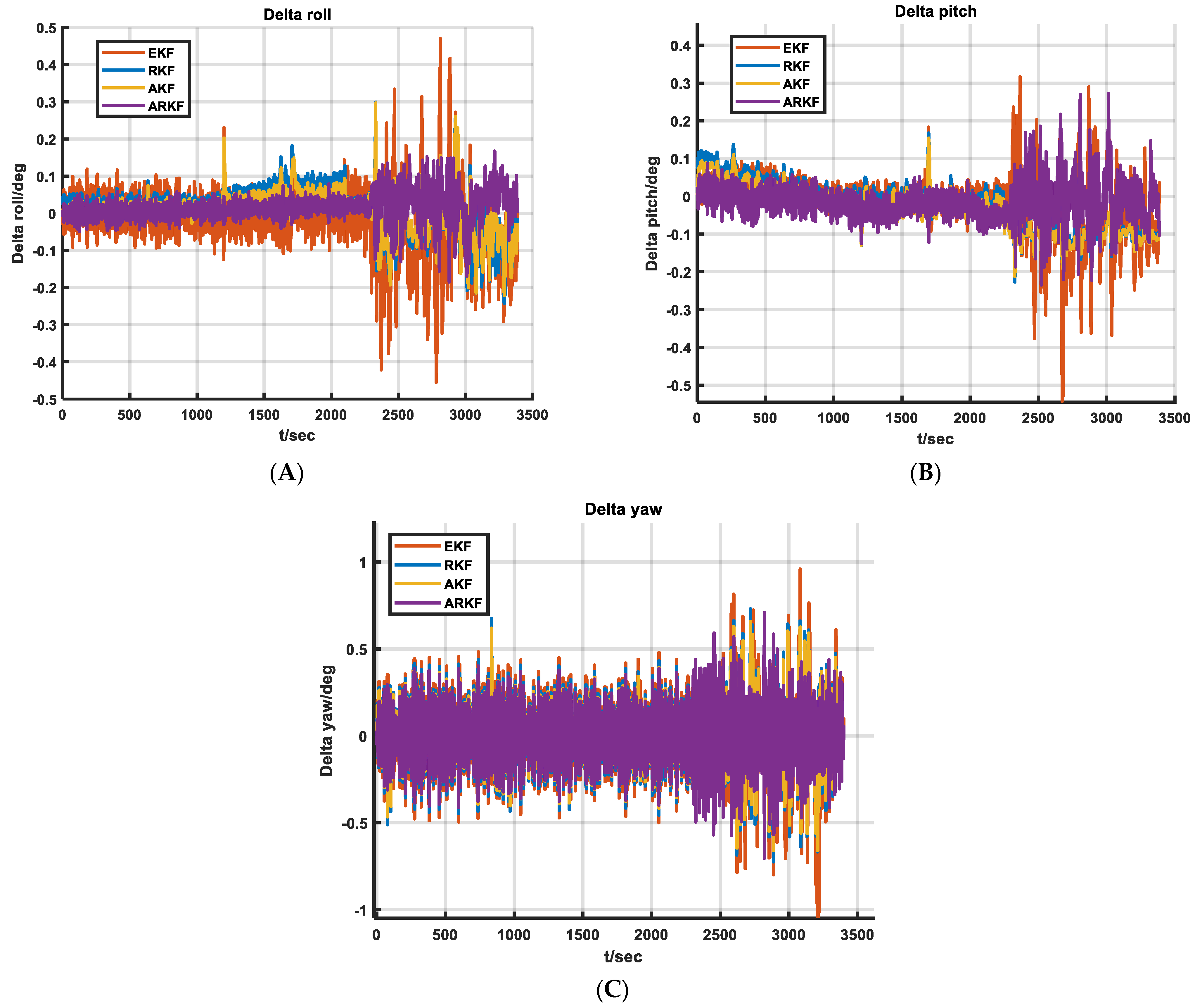
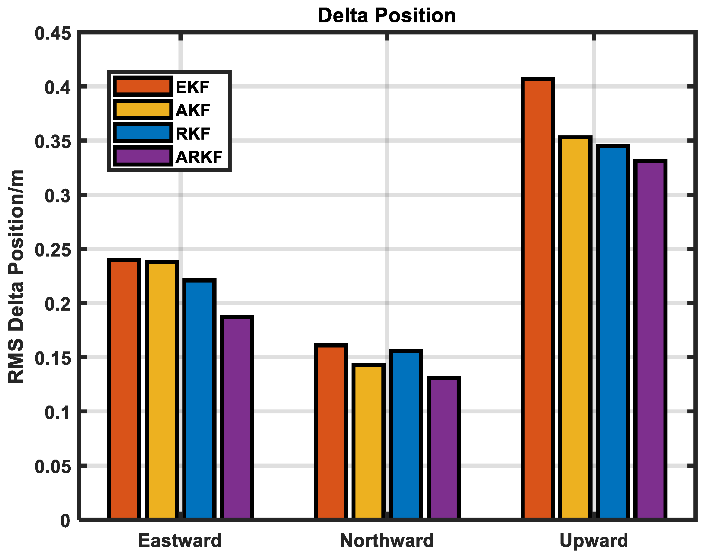
3.3. Shipboard Experiments

The experiment was carried out in the sea area around Changyi, Weifang, China. The experimental scene was a low-speed and high-vibration marine environment. The experiment lasted about 1 h. The ship is equipped with four GNSS antennas, and a main antenna is used as the GNSS solution result. The base station is set up on the coast, and the baseline length is about 20 km, so as to obtain the differential GNSS positioning solution. The specific ship-borne experimental route is shown in Figure 12.

Figure 13A,C show the geometric accuracy factor of the shipborne experimental satellite and the number of satellites participating in the solution. Because there is no satellite occlusion problem under the sea observation condition, the observation condition is better. Figure 13B represents the satellite solution factor (Q) of the sea experiment. Figure 13D shows the change in the adaptive fading factor b in the ship-borne experiment.

Figure 14 shows the change in the ship’s heave with time. For the marine sloshing environment, the influence of the ship’s heave on the positioning accuracy cannot be ignored, and the maximum heave amplitude reaches 1 m. After 2500, the heave amplitude of the ship increases significantly. The SINS is prone to abnormal measurement in the low-speed and high-vibration heave environment, which has a great impact on the estimation of the filter.

In order to verify the accuracy of the algorithm in this paper, four algorithms are selected for analysis. The position, velocity and attitude errors obtained by using the above four methods and professional solution software are shown in Figure 15 and Figure 16.

At around 2000 s, the interference of the ship’s heave motion to the positioning system increases significantly. When the heave motion is enhanced, EKF has insufficient ability to deal with the interference of nonlinear and non-Gaussian distribution, and the error fluctuates greatly. Robust filtering needs to be improved and adapted to the offshore heave vibration environment. The error of the algorithm in this paper can still maintain low amplitude and good stability. Compared with all the algorithms in this paper, this algorithm has the smallest error in the sky direction and the smallest fluctuation of the velocity error curve, which shows that it has better stability in the strong interference environment.

In summary, other algorithms have poor adaptability to dynamic environments. Especially when the heave motion is intensified, the attitude estimation error increases significantly, and even diverges. Whether it is roll angle, pitch angle, or heading angle, the error curve of the algorithm in this paper maintains a small fluctuation under the influence of heave motion (around 2000 s).

In order to further compare the accuracy of the position, velocity, and attitude of the four schemes, the position and velocity error (RMS) is plotted as a histogram (Figure 17), and the corresponding results are also summarized in

Table 4. Shipboard experiment position, velocity, and attitude error comparison and analysis table.

ERROR		EKF	AKF	RKF	ARKF
Velocity (m/s)	Eastward	0.101	0.091	0.084	0.080
	Northward	0.112	0.094	0.086	0.071
	Upward	0.254	0.216	0.209	0.173
Attitude (deg)	Roll	0.181	0.140	0.151	0.107
	Pitch	0.204	0.163	0.141	0.128
	Heading	0.355	0.279	0.321	0.223
Position (m)	Eastward	0.240	0.238	0.221	0.187
	Northward	0.161	0.143	0.156	0.134
	Upward	0.407	0.353	0.345	0.331
	Improved accuracy (%)	19.44%	10.47%	8.28%

.

For ship-borne experiments, it can be seen from Table 4 that the accuracy of the algorithm in three-dimensional position is improved by 19.44% compared with EKF, 10.47% compared with Sage-Husa adaptive filtering, and 8.28% compared with robust filtering. These results show that although the system faces great uncertainty and noise interference in the marine environment with low speed, high vibration and severe heave, the algorithm proposed in this paper can still effectively maintain a high accuracy level.

4. Discussion

The ARKF algorithm can maintain stable and accurate positioning performance in the vehicle environment with poor satellite positioning and the complex marine environment with severe heave. Compared with other algorithms, ARKF algorithm has stronger robustness, better anti-interference ability, and higher application value.

The quantitative correlation between environmental perception (PDOP value, Q value) and state prediction credibility breaks through the coupling problem of traditional filtering noise statistics and disturbance suppression, and it provides a new paradigm for nonlinear filtering theory. Two-factor robust theoretical framework: Through the collaborative optimization of fading factor and residual weight, the stability criterion in the dynamic noise scene is established, and the related results can be extended to the field of multi-sensor fusion. In terms of practical value, high-precision navigation of unmanned systems can be achieved. Vehicle experiments show that the three-dimensional positioning error of ARKF in complex urban areas is less than 0.1 m. Meet the sub-meter precision requirements of unmanned distribution vehicles. In the ship-borne experiment, the heading angle error is less than 0.223, which can support the accurate berthing of autonomous ships.

Limitations of the algorithm in this paper. In the existing research, the collaborative optimization of robust filtering and adaptive filtering can partially suppress the influence of non-Gaussian noise. However, if the statistical characteristics of noise are highly deviated from the preset model, the adaptive mechanism of the algorithm may face the challenge of insufficient convergence speed or lagging weight adjustment. For example, in the vehicle experiment of this paper, when the satellite signal is completely occluded and the inertial sensor noise is suddenly abnormal, the positioning error of ARKF is better than other algorithms mentioned in this paper, but there are still short-term fluctuations. This indicates that extreme non-Gaussian noise may impose higher requirements on the dynamic adjustment range of the fading factor.

Aiming at the limitations, the deep learning method is introduced, and the filtering parameters are adjusted by the online noise characteristic identification network to enhance the real-time modeling ability of non-stationary noise. The weight design is improved, and the robustness factor is optimized by combining more flexible distribution assumptions to improve the robustness to impulse noise.

5. Conclusions

In this study, a dynamic robust filtering framework based on multi-source information fusion is constructed to solve the problem of navigation accuracy attenuation in low-speed and high-vibration environment. The real-time optimization of the fading factor is realized by PDOP-Q-effective satellite number-residual joint criterion, and the double weighting strategy constructed by standardized residuals breaks through the coupling problem of traditional algorithms in measurement noise estimation and dynamic disturbance suppression. The experimental results show that in the urban vehicle scene, the proposed algorithm reduces the RMS value of three-dimensional positioning error by 47.12%, 35.26%, and 9.58%, respectively, compared with EKF, RKF, and AKF, and improves the heading angle accuracy by 42.3%. The mean square error of the velocity vector is reduced by 19.44%, the roll angle tracking delay is shortened by 40 ms, and the continuous failure time of the system is extended from 8.2 s to 23.7 s under strong disturbance conditions.

By establishing a closed-loop correction mechanism for the dynamic noise covariance matrix, the collaborative optimization of robust estimation and adaptive filtering is successfully realized, and the nonlinear mapping law between the observation quality quantification index and the state prediction credibility is revealed. It provides a new solution for the fault-tolerant control of multi-source navigation systems in complex dynamic environments, especially for the high-precision pose estimation requirements of unmanned vehicles in low-frequency and high-vibration coupling scenarios.

References

1. Zhang, Z.; Xiao, G.; Nie, Z.; Ferreira, V.; Casula, G. High-Precision and High-Reliability Positioning, Navigation, and Timing: Opportunities and Challenges. Remote Sens. 2024, 16, 4403. [Google Scholar] [CrossRef]
2. Yang, Y.; Yao, Z.; Mao, Y.; Xu, T.; Wang, D. Resilient satellite-based PNT system design and key technologies. Sci. China Earth Sci. 2025, 68, 669–682. [Google Scholar] [CrossRef]
3. Xu, B.; Wang, X.; Guo, Y.; Zhang, J.; Razzaqi, A.A. A novel adaptive filter for cooperative localization under time-varying delay and non-Gaussian noise. IEEE Trans. Instrum. Meas. 2021, 70, 1–15. [Google Scholar] [CrossRef]
4. Delamer, J.-A.; Watanabe, Y.; Chanel, C.P. Safe path planning for UAV urban operation under GNSS signal occlusion risk. Robot. Auton. Syst. 2021, 142, 103800. [Google Scholar] [CrossRef]
5. Yang, Y.; Dai, Z.; Chen, Y.; Yuan, Y.; Yalikun, Y.; Shang, C. Emerging MEMS sensors for ocean physics: Principles, materials, and applications. Appl. Phys. Rev. 2024, 11, 021320. [Google Scholar] [CrossRef]
6. Yang, Y.; Cui, X. Adaptively robust filter with multi adaptive factors. Surv. Rev. 2008, 40, 260–270. [Google Scholar] [CrossRef]
7. Song, S.; Wu, J. Motion State Estimation of Target Vehicle under Unknown Time-Varying Noises Based on Improved Square-Root Cubature Kalman Filter. Sensors 2020, 20, 2620. [Google Scholar] [CrossRef]
8. Ma, C.; Pan, S.; Gao, W.; Wang, H.; Liu, L. Variational Bayesian-based robust adaptive filtering for GNSS/INS tightly coupled positioning in urban environments. Measurement 2023, 223, 113668. [Google Scholar] [CrossRef]
9. Xiong, J.; Cheong, J.W.; Xiong, Z.; Dempster, A.G.; Tian, S.; Wang, R. Adaptive hybrid robust filter for multi-sensor relative navigation system. IEEE Trans. Intell. Transp. Syst. 2021, 23, 11026–11040. [Google Scholar] [CrossRef]
10. Narasimhappa, M.; Mahindrakar, A.D.; Guizilini, V.C.; Terra, M.H.; Sabat, S.L. MEMS-based IMU drift minimization: Sage Husa adaptive robust Kalman filtering. IEEE Sens. J. 2019, 20, 250–260. [Google Scholar] [CrossRef]
11. Zou, T.; Zeng, W.; Yang, W.; Ong, M.C.; Wang, Y.; Situ, W. An adaptive robust cubature Kalman filter based on Sage-Husa estimator for improving ship heave measurement accuracy. IEEE Sens. J. 2023, 23, 10089–10099. [Google Scholar] [CrossRef]
12. Petrus, P. Robust Huber adaptive filter. IEEE Trans. Signal Process. 1999, 47, 1129–1133. [Google Scholar] [CrossRef]
13. Mao, Y.; Sun, R.; Wang, J.; Cheng, Q.; Kiong, L.C.; Ochieng, W.Y. New time-differenced carrier phase approach to GNSS/INS integration. GPS Solut. 2022, 26, 122. [Google Scholar] [CrossRef]
14. Li, Q.; Zhang, L.; Wang, X. Loosely coupled GNSS/INS integration based on factor graph and aided by ARIMA model. IEEE Sens. J. 2021, 21, 24379–24387. [Google Scholar] [CrossRef]
15. Zhang, Q.; Dai, Y.; Zhang, T.; Guo, C.; Niu, X. Road Semantic-Enhanced Land Vehicle Integrated Navigation in GNSS Denied Environments. IEEE Trans. Intell. Transp. Syst. 2024, 25, 20889–20899. [Google Scholar] [CrossRef]
16. Jiang, C.; Zhang, S.; Li, H.; Li, Z. Performance evaluation of the filters with adaptive factor and fading factor for GNSS/INS integrated systems. GPS Solut. 2021, 25, 130. [Google Scholar] [CrossRef]
17. Song, J.; Li, J.; Wei, X.; Hu, C.; Zhang, Z.; Zhao, L.; Jiao, Y. Improved multiple-model adaptive estimation method for integrated navigation with time-varying noise. Sensors 2022, 22, 5976. [Google Scholar] [CrossRef]
18. Yan, G.; Weng, J. Integrated Inertial Navigation Algorithms and Principles of Integrated Navigation; Northwestern Polytechnical University: Xi’an, China, 2019; ISBN 978-7-5612-6547-5. [Google Scholar]
19. Liu, Y.; Wang, L.; Hu, L.; Cui, H.; Wang, S. Analysis of the Influence of Attitude Error on Underwater Positioning and Its High-Precision Realization Algorithm. Remote Sens. 2022, 14, 3878. [Google Scholar] [CrossRef]
20. Guo, F.; Zhang, X. Adaptive robust Kalman filtering for precise point positioning. Meas. Sci. Technol. 2024, 25, 105011. [Google Scholar] [CrossRef]
21. Yin, Z.; Yang, J.; Ma, Y.; Wang, S.; Chai, D.; Cui, H. A Robust Adaptive Extended Kalman Filter Based on an Improved Measurement Noise Covariance Matrix for the Monitoring and Isolation of Abnormal Disturbances in GNSS/INS Vehicle Navigation. Remote Sens. 2023, 15, 4125. [Google Scholar] [CrossRef]
22. Jiang, Y.; Pan, S.; Meng, Q.; Zhang, M.; Ma, C.; Yu, H.; Gao, W. Multiple faults detection algorithm based on REKF for GNSS/INS integrated navigation. In Proceedings of the International Conference on Guidance, Navigation and Control, Harbin, China, 5–7 August 2022; Springer Nature Singapore: Singapore, 2022; pp. 886–894. [Google Scholar] [CrossRef]
23. Liu, J.; Pu, J.; Sun, L.; He, Z. An approach to robust INS/UWB integrated positioning for autonomous indoor mobile robots. Sensors 2019, 19, 950. [Google Scholar] [CrossRef] [PubMed]
24. Chhabra, A.; Venepally, J.R.; Kim, D. Measurement noise covariance-adapting Kalman filters for varying sensor noise situations. Sensors 2021, 21, 8304. [Google Scholar] [CrossRef] [PubMed]
25. Cheng, Y.; Zhang, S.; Wang, X.; Wang, H.; Yang, H. Kalman Filter with Adaptive Covariance Estimation for Carrier Tracking under Weak Signals and Dynamic Conditions. Electronics 2024, 13, 1288. [Google Scholar] [CrossRef]
26. Li, H.; Medina, D.; Vilà-Valls, J.; Closas, P. Robust variational-based Kalman filter for outlier rejection with correlated measurements. IEEE Trans. Signal Process. 2020, 69, 357–369. [Google Scholar] [CrossRef]
27. Biswas, S.K.; Qiao, L.; Dempster, A.G. Effect of PDOP on performance of Kalman Filters for GNSS-based space vehicle position estimation. GPS Solut. 2017, 21, 1379–1387. [Google Scholar] [CrossRef]
28. Wang, Z.; Song, S.; Jiao, W.; Wei, W.; Zhou, W.; Jiao, G.; Liu, J. A unified PDOP evaluation method for multi-GNSS with optimization grid model and temporal–spatial resolution. GPS Solut. 2024, 28, 36. [Google Scholar] [CrossRef]
29. Chen, C.; Zhu, J.; Bo, Y.; Chen, Y.; Jiang, C.; Jia, J.; Duan, Z.; Karjalainen, M.; Hyyppä, J. Pedestrian Smartphone Navigation Based on Weighted Graph Factor Optimization Utilizing GPS/BDS Multi-Constellation. Remote Sens. 2023, 15, 2506. [Google Scholar] [CrossRef]
30. Jiang, S.; Chen, Y.; Liu, Q. Advancements in Buoy Wave Data Processing through the Application of the Sage–Husa Adaptive Kalman Filtering Algorithm. Sensors 2023, 23, 7298. [Google Scholar] [CrossRef]
31. Rahemi, N.; Mosavi, M.R.; Martín, D. A new variance-covariance matrix for improving positioning accuracy in high-speed GPS receivers. Sensors 2021, 21, 7324. [Google Scholar] [CrossRef]
32. Wang, D.; Dong, Y.; Li, Z.; Li, Q.; Wu, J. Constrained MEMS-based GNSS/INS tightly coupled system with robust Kalman filter for accurate land vehicular navigation. IEEE Trans. Instrum. Meas. 2019, 69, 5138–5148. [Google Scholar] [CrossRef]
33. Knight, N.L.; Wang, J. A comparison of outlier detection procedures and robust estimation methods in GPS positioning. J. Navig. 2009, 62, 699–709. [Google Scholar] [CrossRef]
34. Dong, Y.; Wang, D.; Zhang, L.; Li, Q.; Wu, J. Tightly coupled GNSS/INS integration with robust sequential Kalman filter for accurate vehicular navigation. Sensors 2020, 20, 561. [Google Scholar] [CrossRef] [PubMed]
35. Li, B.; Rizos, C.; Lee, H.K.; Lee, H.K. A GPS-slaved time synchronization system for hybrid navigation. GPS Solut. 2006, 10, 207–217. [Google Scholar] [CrossRef]
36. Chai, D.; Sang, W.; Chen, G.; Ning, Y.; Xing, J.; Yu, M.; Wang, S. A novel method of ambiguity resolution and cycle slip processing for single-frequency GNSS/INS tightly coupled integration system. Adv. Space Res. 2022, 69, 359–375. [Google Scholar] [CrossRef]
37. Instructions for the Software (Inertial Explorer 8.70) Used as the Reference Truth Value in the Comparative Experiment. Available online: https://hexagondownloads.blob.core.windows.net/public/Novatel/assets/Documents/Waypoint/Downloads/GrafNav-GrafNet-User-Manual-870/GrafNav-GrafNet-User-Manual-870.pdf (accessed on 1 April 2025).
Figure 1. SINS/GNSS adaptive robust filtering algorithm based on an improved fading factor.
Remotesensing 17 01449 g001
Figure 2. Selection of adaptive fading factor amplitude adjustment coefficient A.
Remotesensing 17 01449 g002
Figure 3. Improved fading factor adaptive fading algorithm (IAKF).
Remotesensing 17 01449 g003
Figure 4. Robust filtering algorithm.
Remotesensing 17 01449 g004
Figure 5. Hardware time synchronization strategy.
Remotesensing 17 01449 g005
Figure 6. Experimental environment: (a) in-vehicle experiments; (b) shipboard experiments.
Remotesensing 17 01449 g006
Figure 7. Vehicle experiment running trajectory.
Remotesensing 17 01449 g007
Figure 8. Vehicle experiment (A) satellite geometric accuracy factor PDOP, (B) satellite solution quality Q, (C) the number of effective satellite observations, (D) adaptive fading factor.
Remotesensing 17 01449 g008
Figure 9. In the vehicle experiment, (A,C,E) represent the comparative analysis of the position errors of the four algorithms in the three directions of the northeast day. In the vehicle experiment, (B,D,F) represent the speed error comparison and analysis of the four algorithms in the three directions of the northeast day.
Remotesensing 17 01449 g009
Figure 10. In the vehicle experiment, (AC) are the error comparison of the four algorithms in roll, pitch, and yaw, respectively.
Remotesensing 17 01449 g010
Figure 11. Vehicle Experiment Rms: position error.
Remotesensing 17 01449 g011
Figure 12. Shipborne experimental trajectory.
Remotesensing 17 01449 g012
Figure 13. Shipborne experiment. (A) Satellite geometric precision factor PDOP, (B) satellite solution quality Q, (C) the number of effective satellite observations, (D) adaptive fading factor.
Remotesensing 17 01449 g013aRemotesensing 17 01449 g013b
Figure 14. Shipboard heave.
Remotesensing 17 01449 g014
Figure 15. In the ship-borne experiment, (A,C,E) represent the comparative analysis of the position errors of the four algorithms in the three directions of the northeast sky. In the ship-borne experiment, (B,D,F) represent the comparative analysis of the velocity errors of the four algorithms in the three directions of the northeast sky.
Remotesensing 17 01449 g015
Figure 16. In the ship-borne experiment, (AC) are the error comparison of the four algorithms in roll, pitch and, yaw, respectively.
Remotesensing 17 01449 g016
Figure 17. Shipboard experiment Rms: position error.
Remotesensing 17 01449 g017