Detecting the Distribution of Callery Pear (Pyrus calleryana) in an Urban U.S. Landscape Using High Spatial Resolution Satellite Imagery and Machine Learning

Abstract

Using Planetscope imagery, we trained a random forest model to detect Callery pear (Pyrus calleryana) throughout a diverse urban landscape in Columbia, Missouri. The random forest model had a classification accuracy of 89.78%, a recall score of 0.693, and an F1 score of 0.819. The key hyperparameters for model tuning were the cutoff and class–weight parameters. After the distribution of Callery pear was predicted throughout the landscape, we analyzed the distribution pattern of the predictions using Ripley’s K and then associated the distribution patterns with various socio-economic indicators. The analysis identified significant relationships between the distribution of the predicted Callery pear and population density, median household income, median year the housing infrastructure was built, and median housing value at a variety of spatial scales. The findings from this study provide a much-needed method for detecting species of interest in a heterogenous landscape that is both low cost and does not require specialized hardware or software like some alternative deep learning methods.

1. Introduction

Callery pear (Pyrus calleryana Decne.) is indigenous to many parts of eastern Asia and was first introduced to the United States in the early 20th century to study its resistance to fire blight, a disease affecting the common pear (Pyrus communis L.) [1]. By the 1950s, various cultivars had been developed, with one, the Bradford, recognized for its potential as an ornamental tree [1]. The Bradford cultivar was commonly planted in subdivisions shortly after its development in the 1950s and several other cultivars were later developed. Whereas the individual cultivars were thought to be sterile and unable to propagate, it was found with Callery pear that different cultivars can cross-pollinate, and scions of the same tree can cross-pollinate if grafted onto different rootstock [2]. No longer sterile, Callery pear has since spread from many urban and developed areas into natural or recently disturbed areas and is widely considered to be an invasive species in many states in the eastern U.S. [3]. This follows a pattern from other invasive species, whereby introduction and continuous propagule pressure due to sales leads to not only establishment in an area but helps establish the invasiveness of a species [4].

There are three basic elements to invasive species management including prevention, detection, and control [5]. Eliminating an invasive species from a landscape often means the physical eradication or removal of the species, which is not only time and labor intensive, but can be financially restrictive as well. Efforts to reduce the spread and remove invasive species from landscapes across the country have been ongoing for years. However, such tasks are extreme logistical and financial challenges, costs of which can vary widely depending on the targeted species [6]. Management methods may vary depending on the nature of the species [7]. There are major management differences among aquatic and terrestrial species, plants and animals, and other influential characteristics. Agencies and organizations often engage the public through awareness campaigns and offering rewards through buyback programs or other similar programs to help control the population of various species [8].

For established invasive plants, the first step in management is identifying where they are located and predicting where they might spread, which can be challenging. For many invasive plants, the use of satellite or other remotely sensed imagery to identify their presence in a landscape can significantly cut costs and provide a much more comprehensive view of their current spread in the landscape compared to more traditional ground survey methods [9]. Methods to remotely sense invasive species vary widely between the sensor types, the algorithms used, and the target species [10,11]. Combining ground surveys with multi-spectral imagery is still a common method to map invasive species when available imagery has relatively coarse spatial resolution [12,13]. More recent studies have focused on using technological innovations in computing power, sensor types (very-high resolution satellite, UAV, hyperspectral) and classification algorithms (machine learning, deep learning) to more precisely and accurately map invasive species’ distributions [14,15,16]. Invasive species often have unique phenology, knowledge of which when applied in conjunction with imagery acquisition can assist with their identification [17]. Callery pear trees have white flowers and tend to bloom a few weeks before co-occurring native plants. However, they also inhabit a wide ecological niche and can grow under diverse environmental settings, making detection based solely on remotely sensed imagery difficult. Thus, using machine learning in conjunction with remotely sensed data provides a promising way of detecting Callery pear.

There have been many studies on the use of machine learning, deep learning, and other artificial intelligence techniques to identify invasive plants in various taxonomic genera and landscape types. While these approaches have proven effective, they often rely on the use of high-resolution data from UAVs or commercial satellites to increase the chance that the target species is identifiable from the imagery and employ analysis frameworks such as deep learning techniques like convolutional neural networks (CNN) [15,16,18,19,20]. For example, one such study used 4-band aerial imagery to identify Callery pear within New York City and compared a pixel-based filtering method and two CNN methods [20]. The pixel-based filtering method that was applied had a very high error rate, but the two CNN methods were each more effective, with over 80% precision, recall, and F1 scores each, but notably, the first method took ~7 h to run just for Staten Island and the second ~36 h to run across the entire study area [20]. Whereas the methods from these studies have proven effective, high-resolution imagery from UAVs and commercial imagery vendors can be costly and, in the case of UAVs, may require special permission to be flown over some areas along with several other limitations. CNN frameworks can require hardware, software, and expertise that may not be easily accessible by researchers and land managers. As such, there is a need for methods that can be utilized by researchers and managers regardless of budget or access to costly computing resources that works with imagery that is readily available, affordable, and frequently captured so that vegetation changes over time can be better monitored.

To this end, Planetscope imagery is explored as a potential data source for identifying invasive vegetation. Planetscope imagery is freely available under a research license with a spatial resolution of 3.0 m, high enough to identify individual Callery pear trees or small patches of escaped trees throughout a diverse, heterogeneous landscape. There are eight spectral bands in Planetscope imagery ranging from coastal blue (443 nm) to near infrared (865 nm). We also chose imagery that was orthorectified and corrected for geometric, radiometric, and surface reflection, making the images suitable for analysis.

Observations of Callery pear were inventoried and geolocated in an urbanized area in Central U.S. A random forest (RF) machine learning approach that requires no specialized computing equipment (e.g., graphical processing units (GPUs)) was then used to predict Callery pear locations from Planetscope images. The distribution of invasive species such as Callery pear is influenced by both environmental and human factors. In this study, we analyze the spatial distribution of predicted Callery pear trees across the study area and examine the relationship between the spatial distribution of the trees and socio-economic variables at the census tract level. The socio-economic variables used for this analysis included population density, median household income, median home value, and median year of housing unit construction. Because the Callery pear was widely planted in housing developments for a span of a few decades between 1960 and 2000, we hypothesized that census tracts with a median year of housing unit construction within this period would exhibit greater clustering of Callery pear, as trees planted in newly developed lots may have subsequently spread to nearby disturbed areas. Additionally, we expected median household income and median home value to have positive relationships with observed clustering. Areas with higher household income and higher household value are more likely to have single-family housing units with larger lots for ornamental tree planting, as well as more open space for the species to spread. Conversely, we anticipated a negative correlation between population density and tree clustering, as denser areas tend to have either higher urban development, limited suitable planting space, or a higher proportion of undisturbed land, which may restrict the trees’ ability to spread. Finally, the management implications of the analysis are discussed.

2. Materials and Method

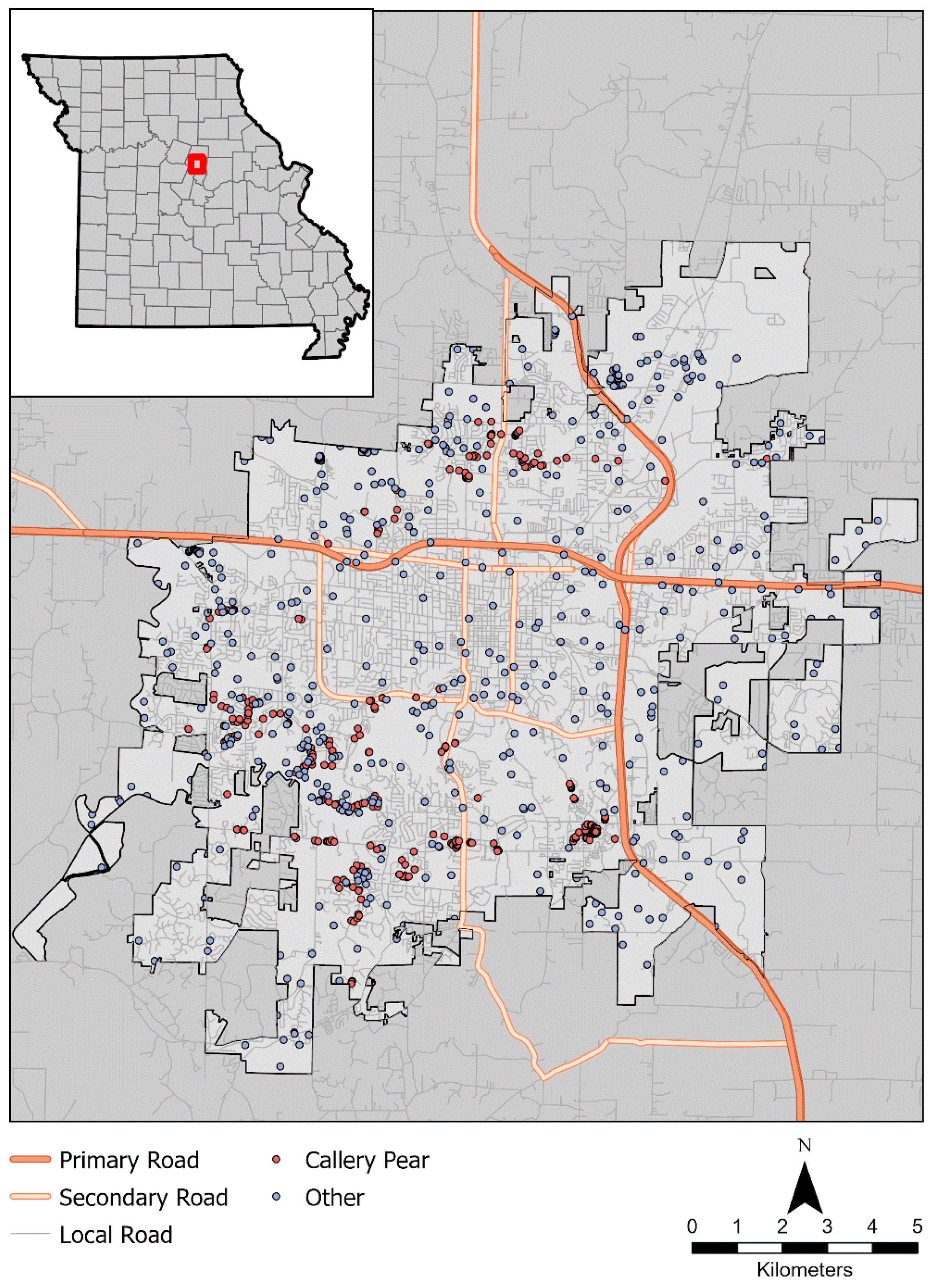
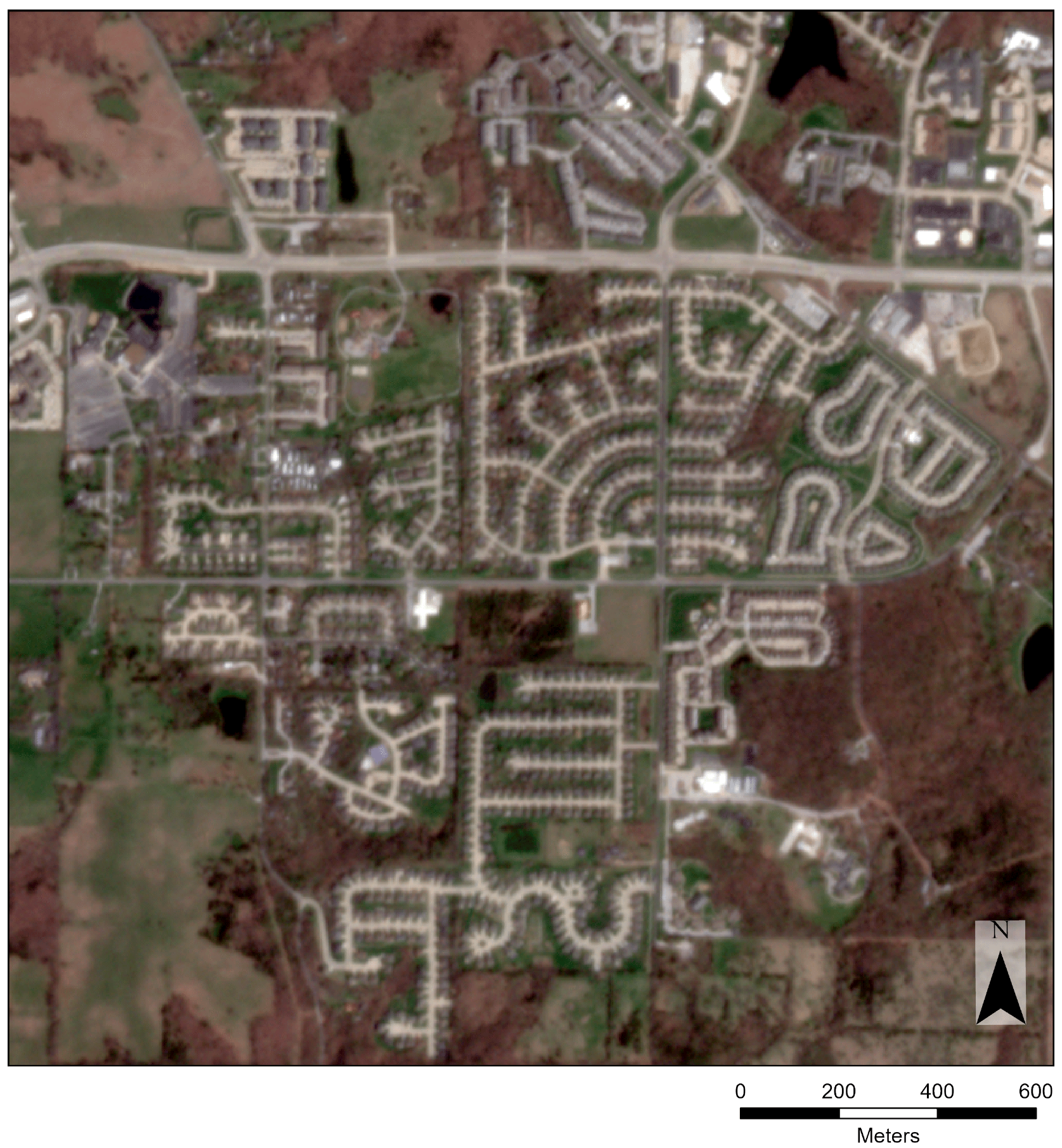
2.1. Study Area

The city of Columbia, MO, USA was selected as the region of interest for this study as it is home to the United States Forest Service (USFS) Northern Research Station and Callery pear has been identified by researchers as a pervasive problem within the city. Columbia has an approximate population of 126,172 and covers an area of 174.3 km² [21]. Within Columbia, the dominant land cover class is developed, low intensity (19.8%), followed by developed, medium intensity (15.3%) and pasture/hay (15.2%) [22]. Columbia is rapidly urbanizing with much development occurring in areas that were previously agricultural, which may facilitate the spread of invasive plants through disturbed habitats and new open potential travel corridors.

2.2. Field Sampling and Training Data

The U.S. Census Bureau TIGER place boundaries from 2021 were used to define the extent of the city [23]. The location of Callery pear trees in the city were recorded using global positioning systems (GPS) (Garmin Ltd., Olathe, KS, USA), in April of 2022 and April 2023. Callery pear trees were in bloom at these times and the location of those that were easily identifiable from the road were recorded. When possible, points were collected directly at the tree or patch of trees; however, there were times when points were collected near the tree with notes taken to indicate the orientation and the distance from the GPS point to the tree. For example, this was performed in cases where the tree was on private property, or if there were safety concerns. After collection, the GPS points were visualized using ArcGIS Pro (version 2.7) a geographic information system (GIS),to compare the location of the points relative to the location of the targeted trees in a satellite imagery basemap and in accordance with notes taken about the GPS point [24]. If a point could not be positively associated with a tree or patch, then it was excluded from the final training dataset. After cleaning the data, 225 observations of Callery pear were retained. There were 75 additional Callery pear points identified for a section of Columbia where the imagery basemap clearly captured some other trees in bloom for which field observations were not collected [24]. In total, 300 observations of Callery pear locations were retained for use in model training.

Next, 500 randomly distributed points within the city boundaries of Columbia were generated using GIS to be used in the training process as a second class. No points were generated within 10 m of inventoried Callery pear sites to avoid points being generated for a documented tree. These points were then appended to the Callery pear point dataset. A field was added to identify the points as ‘Callery pear’ or ‘other’. To account for features that contributed to incorrect classification, 100 ‘other’ points were added to define various roads and fields that were often confused as Callery pear in early iterations of the model. In total, the final training data set contained 300 Callery pear points and 600 other points (Figure 1).

2.3. Planetscope Data

Planetscope is a constellation of 430+ satellites (CubeSats) that provides imagery with a daily return around the Earth [25]. Planetscope imagery from 8 April 2023 corresponding with the timing of ground data collection and the blooming season was acquired. Additional images from 11 August and 20 October 2023 were collected for model training to capture the spectral differences between the Callery pear and surrounding vegetation during late summer and early autumn. All acquired imagery had 0% cloud cover over the study area and were level 3B products, meaning the scenes were orthorectified and corrected for geometric, radiometric, and surface reflection [25].

From each image, key spectrum reflectance indices were calculated as shown in

Table 1. Spectrum reflectance indices calculated in the study where NIR is near-infrared band reflectance (845–885 nm), R is red band reflectance (650–680 nm), G is green band reflectance (547–583 nm), B is blue band reflectance (465–515 nm), and Y is yellow band reflectance (600–620 nm).

Spectral Vegetation Indices	Calculation
Normalized Difference Vegetation Index	(NIR − R)/(NIR + R)
Green Normalized Difference Vegetation Index	(NIR − G)/(NIR + G)
Green–Red Ratio	(G − R)/(G + R)
Green–Yellow Ratio	(G − Y)/(G + Y)
Modified Soil-Adjusted Vegetation Index	${\displaystyle \frac{\left(2\ast NIR+1-\sqrt{{(2\ast NIR+1)}^2-8\ast \left(NIR-R\right)}\right)}{2}}$
Transformed Chlorophyll Absorption in Reflectance Index	${\displaystyle \frac{(3\ast \left(NIR-R\right)-2\ast (B-R\left)\right)}{(\left(NIR+R+0.5\right)\ast \left(1+0.5\right))}}$
Visible Atmospherically Resistant Index	(G − R)/(G + R − B)
Scene ‘Whiteness’	R + G + B

and

Table 2. Spectrum reflectance texture indices calculated in the study where i,j is the row, column indices for image pixels, P(i,j) is probability of pixel pair (i,j) in the gray-level co-occurrence matrix, Mean is the average gray-level intensity of the image, and ε is a small constant to avoid taking the logarithm of zero.

Texture Indices	Calculation
Gray-Level Co-Occurrence Matrix–Mean	${\displaystyle \sum _{i,j}}P\left(i,j\right)\cdot \left(i+j\right)$
Gray-Level Co-Occurrence Matrix–Variance	${\displaystyle \sum _{i,j}}P\left(i,j\right)\cdot [\left(i+j\right)-Mean{]}^2$
Gray-Level Co-Occurrence Matrix–Homogeneity	${\displaystyle \sum _{i,j}}{\displaystyle \frac{P\left(i,j\right)}{1+|i-j|}}$
Gray-Level Co-Occurrence Matrix–Entropy	${\displaystyle \sum _{i,j}}P\left(i,j\right)\cdot {\mathit{log}}_2\left(P\left(i,j\right)+\epsilon \right)$

and used in the training of the random forest model.

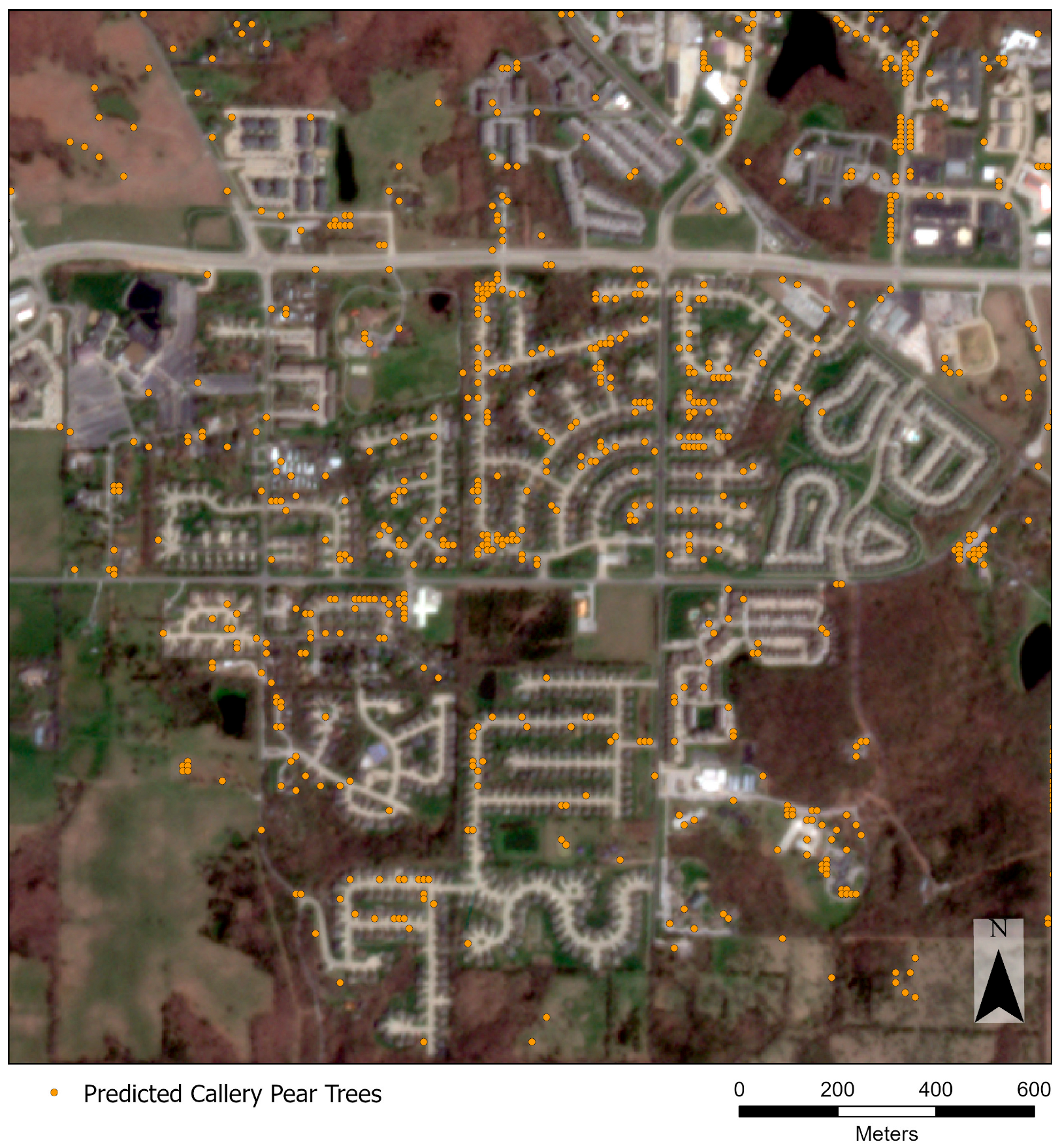
2.4. Machine Learning

Random forest is a non-parametric decision tree method, meaning that decision trees are built with no assumption about the distribution of the data. Random forest builds trees by randomly selecting a subset of the training variables into sets of unique decision trees and trains each tree on the selected subset of the variables for that tree. The predictions of all the decision trees are then aggregated to improve the overall accuracy of the classification. This method provides a randomized variable input which helps to reduce overfitting [26]. For this application, the vegetation and texture indices calculated for each image (April, August, and October) seen in Table 1 and Table 2 were used, as well as the difference in the indices’ values between April and August and between April and October, resulting in a total of 60 variables used to train the model. The chosen spectral indices were used as model inputs because they provide a comprehensive set of vegetation, spectral, and texture-related features that help differentiate land cover types based on their unique reflectance patterns and structural characteristics. These indices capture various aspects of vegetation health, canopy structure, and surface texture, making them suitable for improving classification accuracy in remote sensing applications [17,18].

Random forest has several hyperparameters that can be tuned by the user. Hyperparameters were selected by iteratively adjusting one at a time while keeping others constant, allowing for a clear assessment of each parameter’s impact on model performance. The final values were chosen based on the configuration that yielded the highest performance on validation data. For this implementation of random forest, we used the randomforest package in R (version 4.3.1) [27]. One of the primary hyperparameters of the random forest model that can be tuned by the user is the number of trees the model builds. The default value for the number of trees in this implementation is 500 and after experimentally adjusting this parameter, we settled on using the default 500 trees as there was no major benefit to increasing the number of trees to the model’s performance. The node parameter caps the size of the tree by setting a minimum number of data points required in each final group (or terminal node). The default value is 1.0, meaning that each terminal node can have just one data point. Increasing this number ensures that each split must contain more data, making the tree smaller and less complex. This helps reduce overfitting and leads to better model generalization. After experimentation, the node parameter was set to 15.0 in the final model for this application. The mTry parameter is the number of features to consider when creating each tree. For classification, the default for this parameter is the square root of the number of possible features. With 60 input features, the default would have been 7.7, but after tuning, mTry was set to 15.0 for this application. The class–weight parameter allows the user to assign weights to different classes, providing more consideration to under-represented classes in the training set. The default is to weight each class equally; however, in this application the weight of the Callery pear observations was set to 10.0 and the weight of the randomly assigned points was set to 1.0. The final parameter that was manually tuned was the cutoff parameter, which sets the threshold probability to classify observations into different classes. The default is 1 divided by the number of classes, which in this application would be 0.5 since there were two classes. After tuning, the cutoff for the Callery pear observations was adjusted to be 0.85 while that of the random points was set to 0.15.

Each of these variables were tuned manually through empirical evaluation. The hyperparameters with the biggest impact on the overall predictive performance of the model were the class weights and cutoff values. Class weights were increased to 10.0 for the Callery pear class, partially to account for an imbalance in the dataset where the ‘other’ class had twice the frequency of the ‘Callery pear’ class, but also to account for the relatively small amount of Callery pear that occurs in the landscape. Since there is a natural imbalance of classes, weighting the features helped improve the model’s overall predictive performance. The cutoff value was difficult to determine. By default, the cutoff value is 0.50 in a two-class classification using random forest. We found that this default value produced a lot of visual noise, meaning that some obvious false Callery pear predictions were included in the final results. For example, areas surrounding a correct prediction were often also labeled as Callery pear, even when they were roads or rooftops. This occurred despite the model’s performance metrics being very strong. By increasing the cutoff to 0.85, this meant that 85% of the trees in the model would need to predict the class as being ‘Callery pear’ for it to be predicted as such in the final model. While this lowered the model’s performance metrics, we found that there was much less noise in the predictions.

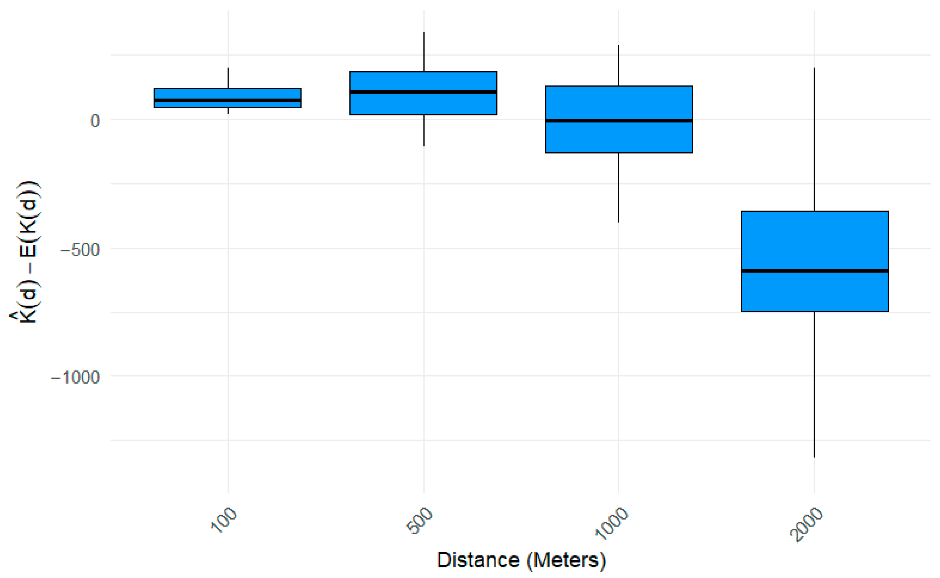
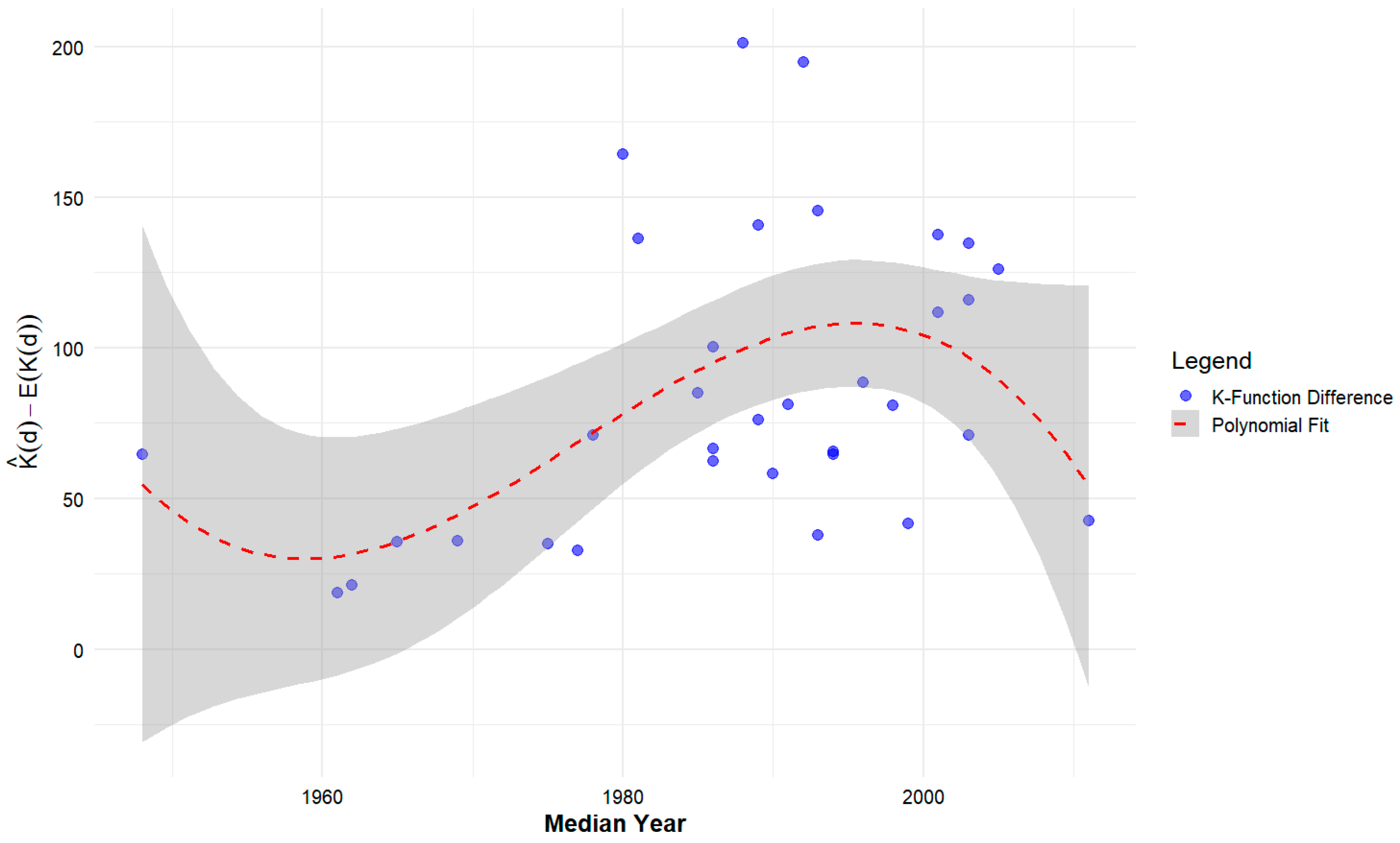
2.5. Spatial Pattern Analysis

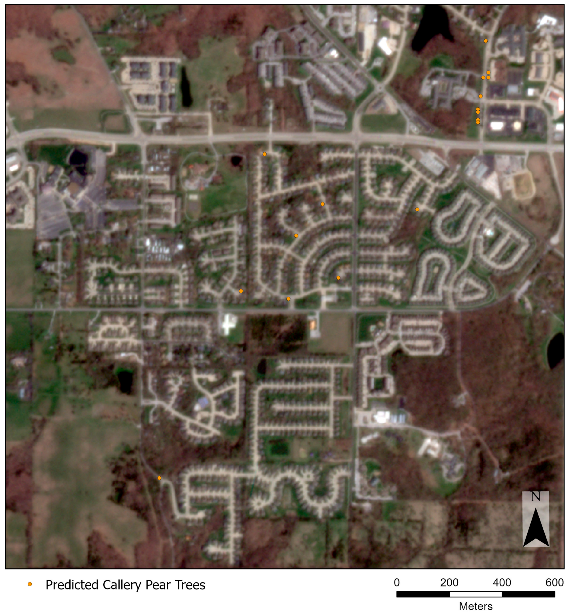
To examine the spatial pattern of Callery pear, the 3.0 m raster output of our random forest prediction was resampled to a 10.0 m using the nearest neighbor method. This was performed so that a single large tree would not have multiple points associated with it when performing the cluster analysis. Cells from the 10.0 m raster that were predicted to be Callery pear were then converted to points. The predicted trees were then used as the input to the Ripley’s K function. Ripley’s K function analyzes the clustering or dispersion of point features within distance (d) using the following formula [28]:

$$K\left(d\right)=\sqrt{{\displaystyle \frac{A{\sum }_{i=1}^n{\sum }_{j=1,j\ne i}^n{k}_{i,j}}{\pi n(n-1)}}}$$

where K(d) represents the K function value given a specific distance d, A is the total area represented by the features, n is the number of features, and k_i,j is a weight equal to 1.0 if the distance between feature i and j is less than d, or 0.0 otherwise. The output of Ripley’s K function is the distance, the expected K values $E\left(K\left(d\right)\right),$ and the observed K values $\widehat{K}\left(d\right)$ as well as the upper and lower confidence levels to determine significance. An observed value above the upper confidence level indicates clustering, while an observed value below the lower confidence level indicates dispersion. The difference between the observed and expected K values ($\widehat{K}\left(d\right)-E\left(K\left(d\right)\right))$ can also be assessed, with a difference above zero indicating more clustering at the indicated distance and a difference below zero indicating dispersion.

Ripley’s K analysis was computed within each Census tract within the study area so that the results could be associated with the socio-economic variables of that tract. K(d) was computed for d = 100 m to d = 2000 m at 100 m increments (i.e., $\{100+100t|t\in \{0,1,\dots ,19\}\}$). The 100-m increment was chosen to capture fine-scale clustering patterns while ensuring meaningful differentiation between distances. Setting the number of distance increments to 20 allowed for a sufficient range of analysis, balancing computational efficiency with the ability to detect spatial clustering trends over varying distances. This approach ensures that both small-scale and broader spatial patterns of Callery pear distribution are effectively captured. Finally, the confidence envelope at the 99% confidence level was computed to examine the statistical significance of any patterns. These parameters allow us to examine how the clustering tendencies change given distances of 100 m to 2000 m.

After the cluster analysis, several socio-economic variables from the American Community Survey (ACS) 5-year estimates for the years 2018–2022 were joined to each Census tract [29]. These variables included the percent of the median household income, median housing unit build year, median housing unit value, and population density. These variables were chosen as they may each have unique correlations with land use patterns, infrastructure, landscaping practices, human activity levels, and urbanization which may contribute in different ways to the spread of invasive species such as Callery pear. For each of these variables, a correlation analysis with the difference between the observed and expected K values from the cluster analysis was performed.

3. Results

After resampling the model output raster and converting to points to be used in the cluster analysis, the model detected 13,744 individual trees or patches throughout the landscape. The random forest classification had an overall accuracy of 89.78%. With no false positives in the model, precision of the model was 1 and recall was 0.693 with an F1 score of 0.819 (

Table 3. Final random forest model confusion matrix.

	Callery Pear	Other	Class Error
Callery pear	208	92	30.6%
Other	0	600	0.0%

). Recall is a measure of the model’s ability to identify true positives, meaning that the model correctly identified nearly 70% of the trees in the training data set. The F1 score is the harmonic mean of precision and recall. A score of 0.819 indicates the model maintains a good balance between identifying Callery pear in the landscape and avoiding false positives.

Random forest produces importance scores for each variable that are used to train the model but does not explain how the features influence the target variable, only that they were used in splitting decisions. Contrary to what was expected, the scene whiteness index (Table 1) in April was not the most important variable, but rather it was the whiteness score for August. The second most important factor was the NDVI difference between April and August, and the third most important factor was the VARI difference between April and August. The whiteness score for April was the ninth most important factor. The least important factors were both differences in texture indices that quantify the uniformity of pixel intensity values in an image, the Gray-Level Co-Occurrence Matrix–Homogeneity difference between April and August and Gray-Level Co-Occurrence Matrix–Homogeneity difference between April and October.

After applying Ripley’s K cluster analysis to the predicted trees, we found statistically significant clustering, meaning that Callery pear trees were more spatially concentrated than would be expected under a random distribution. This clustering was observed both across the entire study area and within individual census tracts, with significant patterns persisting up to 300 m. At a distance of 500 m, most census tracts still exhibited significant clustering, but some started to show dispersion instead of clustering, indicating a more spread-out distribution of trees at this spatial scale. At a distance of 1000 m, census tracts were nearly evenly split between clustering and dispersion; however, at a distance of 2000 m the majority of census tracts exhibited significant dispersion, suggesting that when examined at larger spatial scales, Callery pear is more evenly distributed rather than forming dense clusters (Figure 2).

When comparing the difference between expected K and the observed K, $\widehat{K}\left(d\right)-E\left(K\left(d\right)\right)$ with socio-economic variables, it was found that it had significant correlation with all variables that we checked across the different spatial scales (

Table 4. $\widehat{K}\left(d\right)-E\left(K\left(d\right)\right)$ associations with various socio-economic variables where d represents the distance (m) of analysis. Significance levels are denoted as follows: *** p < 0.001 (highly significant), ** p < 0.01 (strongly significant), and * p < 0.05 (statistically significant). Values without asterisks are not statistically significant (p ≥ 0.05). Positive correlation coefficients (r) indicate that as the socio-economic variable increases, the difference between observed K and expected K also increases.

Variable	d	Correlation Coefficient (r)	Model Type	Adjusted R2
Median Household Income	100	0.397 *	Linear Regression	0.1313 *
	500	0.499 *		0.2252 **
	1000	0.566 **		0.2989 ***
	2000	0.640 ***		0.3907 ***
Median Year Built	100	0.364 *	Polynomial Regression (third degree)	0.1758 *
	500	0.324		0.2542 **
	1000	0.387 *		0.3113 **
	2000	0.399 *		0.2878 **
Median Value	100	0.3773 *	Linear Regression	0.1156 *
	500	0.5449 **		0.2749 ***
	1000	0.5680 **		0.3014 ***
	2000	0.6010 **		0.3411 ***
Population Density	100	−0.5597 **	Linear Regression	0.2919 ***
	500	−0.727 ***		0.5148 ***
	1000	−0.778 ***		0.5926 ***
	2000	−0.785 ***		0.604 ***
Combined	100		Linear Regression	0.3344 **
	500			0.5497 ***
	1000			0.6746 ***
	2000			0.7182 ***

). Median household income, median year built, and median value all had positive correlations with $\widehat{K}\left(d\right)-E\left(K\left(d\right)\right)$ across all spatial scales (Table 4). It is important to remember when interpreting this relationship that Ripley’s K values above zero indicate clustering, while values below zero indicate dispersal. Since at a distance of 500 m $\widehat{K}\left(d\right)-E\left(K\left(d\right)\right)$ starts to change from positive to negative for most census tracts, at greater distances such as 2000 m we would say that as the values for these socio-economic variables increase, the degree of dispersion decreases, whereas at a spatial scale of 200 m, as these socio-economic variables increase, clustering tends to increase. Population density was significantly negatively associated with $\widehat{K}\left(d\right)-E\left(K\left(d\right)\right)$ at all distances, meaning that as population density increases, clustering is reduced, and at greater distances dispersion is increased.

4. Discussion

Overall, the developed approach worked well to predict the distribution of 13,744 Callery pear trees and small patches throughout the city of Columbia. In the early stages of this work, the number of trees, nodes, and mtry (the number of features used to build each tree) were the primary hyperparameters for model tuning. The resulting performance measures were very good, with over 90% overall classification accuracy. However, when the model was applied across the landscape, the predictions included significant noise. By adjusting the class weights and cutoff hyperparameters, we were able to discern the predicted classification results of isolated individual trees or patches. In particular, the cutoff hyperparameter made a large difference in limiting noise in the prediction noise. Figure 3, Figure 4, Figure 5 and Figure 6 illustrate the imagery and predictions for a small portion of the study region.

Initially when tuning the cutoff hyperparameter value, we tried a cutoff parameter value of 0.75 for the Callery pear class, meaning that 75% of the trees in the model had to agree the pixel was a Callery pear (Figure 4). Although the model performance appeared to have improved, the raster produced by the prediction still contained considerable noise (

Table 5. Confusion matrix with 0.75 cutoff value, meaning 75% of the trees built in the model must agree that a pixel is ‘Callery pear’ for it to be classified as such, and 0.95 cutoff value, meaning that 95% of the trees built in the model must agree that a pixel is ‘Callery pear’ for it to be classified in the final model as one.

	Cutoff	Callery Pear	Other	Class Error
Callery pear	0.75	264	36	12.0%
Other	0.75	0	600	0.0%
Callery pear	0.95	92	208	69.3%
Other	0.95	0	600	0.0%

).

When the cutoff value was increased to 0.95, the model then missed too many valid trees (Figure 6), and overall model performance decreased (Table 5). At a value of 0.85, the model still exhibited good performance (Table 1) and the level of noise in the resulting prediction was acceptable (Figure 5).

The variables that were the most important to the model ranged between imagery months and index type (vegetation or texture indices). This is in line with other studies that have found that using muti-temporal imagery for species classification provides better results by capitalizing on phenology differences [16,19,30,31]. Various combinations of imagery months and indices were experimented with, but it was consistently found that results were better using imagery from when the trees were in bloom, a summer month, and a fall month and using all indices for each image.

One interesting finding was that the ‘Whiteness’ score for August and October was more important to the model than that of April, despite the use of from when Callery pear was in bloom with white flowers. We expected the whiteness in April combined with vegetative indices in April to have the most influence on the model. This may be due to other white features in the landscape, such as white concrete roads in subdivisions, being more useful in splitting decisions than the blooming trees in April. Since Callery pear is relatively scarce compared to all other land cover in the landscape, the natural imbalance of the classes could further contribute to the whiteness score in August being the most important factor due to a relatively high number of white pixels from non-vegetation sources being used for splitting decisions.

The observed negative correlation between Callery pear clustering and population density suggests that urbanized areas with higher densities may act as natural barriers to the species’ spread due to limited suitable habitat and consistent landscaping practices. However, this does not mean these areas are immune to invasion, as ornamental plantings in urban settings can still serve as seed sources for spread into nearby disturbed areas. Management strategies in these regions should focus on preventing the intentional planting of Callery pear in urban landscaping, implementing replacement programs with non-invasive alternatives, and promoting public awareness campaigns about the tree’s invasive nature. Conversely, lower-density areas, particularly those undergoing development or land-use change, are at greater risk for Callery pear establishment and spread. Given the tree’s strong association with disturbed landscapes [3], management efforts should prioritize monitoring and early detection in these transitional zones, especially along roadsides, abandoned lots, and newly cleared land. Proactive removal efforts in these areas could prevent the establishment of seed banks and mitigate further spread. Additionally, the polynomial relationship between median year built and Callery pear prevalence suggests that neighborhoods constructed in the 1990s experienced a peak in ornamental planting, making them particularly vulnerable to established populations (Figure 7). We recognize that this relationship may not perfectly capture the spread of the data, especially in the center of the range; however, it provides a useful approximation of the general pattern. Additionally, the observed deviations in the center range suggest that other factors play a role in the establishment of Callery pear in these areas. Neighborhoods built in this time frame should be considered high-priority areas for intervention, including targeted removal programs, homeowner engagement initiatives, and incentives for replacing Callery pear with native or non-invasive species. Municipal and homeowner association policies could also be leveraged to encourage removal and replacement efforts. By focusing on both urban and suburban areas, these targeted management interventions can help mitigate the continued spread of Callery pear and reduce its ecological impact.

5. Conclusions

Our objectives for this analysis were to predict Callery pear locations throughout Columbia, correlate the distribution patterns with various socio-economic variables, and then use this information to discuss management implications, such as targeting buy-back programs or removal efforts. To this end, a random forest model, an accessible machine learning algorithm, was employed to predict Callery pear using a source of high-resolution imagery that can be obtained at little to no cost to practitioners in governmental and academic institutions. This approach for identifying Callery pear in a mixed urban landscape using random forest and multitemporal, high resolution PlanetScope imagery was one of the first such attempts to our knowledge. Prior identification of Callery pear using 4-band aerial imagery and a CNN was recently performed, with CNN results comparable to that of the random forest model utilized in this study [20]. Another major difference between the two approaches is that this study utilizes multitemporal, 8-band imagery (versus 4-band single date imagery) and a coarser image resolution (3 m versus 15.2 cm) [20]. With an overall accuracy of 89.1% and a Callery pear class accuracy of 69.6%, we were able to identify 13,744 individual trees and small patches of both planted and escaped trees throughout a complex, urban landscape. This approach is very cost effective as the imagery is available for free for research purposes for university affiliated researchers, and Planet has additional programs for non-profits and federal government researchers that could help reduce overhead costs for others interested in utilizing imagery from Planet. However, further experimentation is needed to determine the extent to which this particular modeling approach could be applied to other cities or regions. Future work could extend these methods to other invasive plants such as bush honeysuckle (Lonicera spp.) and autumn olive (Elaeagnus umbellata Thunb.). Additional model enhancements such as controlling for climate zone and city characteristics could further broaden the geographic applicability of this approach.

References

1. Culley, T.M.; Hardiman, N.A. The Beginning of a New Invasive Plant: A History of the Ornamental Callery Pear in the United States. BioScience 2007, 57, 956–964. [Google Scholar] [CrossRef]
2. Culley, T.M.; Hardiman, N.A.; Hawks, J. The role of horticulture in plant invasions: How grafting in cultivars of Callery pear (Pyrus calleryana) can facilitate spread into natural areas. Biol. Invasions 2011, 13, 739–746. [Google Scholar] [CrossRef]
3. Vincent, M.A. On the Spread and Current Distribution of Pyrus calleryana in the United States. Castanea 2005, 70, 20–31. [Google Scholar] [CrossRef]
4. Fertakos, M.E.; Bradley, B.A. Propagule pressure from historic U.S. plant sales explains establishment but not invasion. Ecol. Lett. 2024, 27, e14494. [Google Scholar] [CrossRef]
5. Rejmánek, M. Invasive plants: Approaches and predictions. Austral Ecol. 2000, 25, 497–506. [Google Scholar] [CrossRef]
6. Januchowski-Hartley, S.R.; Visconti, P.; Pressey, R.L. A systematic approach for prioritizing multiple management actions for invasive species. Biol. Invasions 2011, 13, 1241–1253. [Google Scholar] [CrossRef]
7. Pile Knapp, L.; Coyle, D.; Dey, D.; Fraser, J.; Hutchinson, T.; Jenkins, M.; Kern, C.; Knapp, B.; Maddox, D.; Pinchot, C.; et al. Invasive plant management in eastern North American Forests: A systematic review. For. Ecol. Manag. 2023, 550, 121517. [Google Scholar] [CrossRef]
8. Haley, A.L.; Lemieux, T.A.; Piczak, M.L.; Karau, S.; D’addario, A.; Irvine, R.L.; Beaudoin, C.; Bennett, J.R.; Cooke, S.J. On the effectiveness of public awareness campaigns for the management of invasive species. Environ. Conserv. 2023, 50, 202–211. [Google Scholar] [CrossRef]
9. Thapa, B.; Darling, L.; Choi, D.; Ardohain, C.; Firoze, A.; Aliaga, D.; Hardiman, B.; Fei, S. Application of multi-temporal satellite imagery for urban tree species identification. Urban For. Urban Green. 2024, 98, 128409. [Google Scholar] [CrossRef]
10. Joshi, C.; De Leeuw, J.; van Duren, I.C. Remote sensing and GIS applications for mapping and spatial modelling of invasive species. In Proceedings of the XXth ISPRS Congress: Geo-Imagery Bridging Continents, Istanbul, Turkey, 12–23 July 2004; Volume 35. [Google Scholar]
11. Papp, L.; van Leeuwen, B.; Szilassi, P.; Tobak, Z.; Szatmári, J.; Árvai, M.; Mészáros, J.; Pásztor, L. Monitoring Invasive Plant Species Using Hyperspectral Remote Sensing Data. Land 2021, 10, 29. [Google Scholar] [CrossRef]
12. Resasco, J.; Hale, A.N.; Henry, M.C.; Gorchov, D.L. Detecting an invasive shrub in a deciduous forest understory using late-fall Landsat sensor imagery. Int. J. Remote Sens. 2007, 28, 3739–3745. [Google Scholar] [CrossRef]
13. Robinson, T.P.; Wardell-Johnson, G.W.; Pracilio, G.; Brown, C.; Corner, R.; van Klinken, R.D. Testing the discrimination and detection limits of WorldView-2 imagery on a challenging invasive plant target. Int. J. Appl. Earth Obs. Geoinf. 2016, 44, 23–30. [Google Scholar] [CrossRef]
14. Kattenborn, T.; Lopatin, J.; Förster, M.; Braun, A.C.; Fassnacht, F.E. UAV data as alternative to field sampling to map woody invasive species based on combined Sentinel-1 and Sentinel-2 data. Remote Sens. Environ. 2019, 227, 61–73. [Google Scholar] [CrossRef]
15. Lake, T.A.; Briscoe Runquist, R.D.; Moeller, D.A. Deep learning detects invasive plant species across complex landscapes using Worldview-2 and Planetscope satellite imagery. Remote Sens. Ecol. Conserv. 2022, 8, 875–889. [Google Scholar] [CrossRef]
16. Nininahazwe, F.; Théau, J.; Marc Antoine, G.; Varin, M. Mapping invasive alien plant species with very high spatial resolution and multi-date satellite imagery using object-based and machine learning techniques: A comparative study. GIScience Remote Sens. 2023, 60, 2190203. [Google Scholar] [CrossRef]
17. Bradley, B.A. Remote detection of invasive plants: A review of spectral, textural and phenological approaches. Biol. Invasions 2014, 16, 1411–1425. [Google Scholar] [CrossRef]
18. Fang, F.; McNeil, B.; Warner, T.; Maxwell, A.; Dahle, G.; Eutsler, E.; Li, J. Discriminating tree species at different taxonomic levels using multi-temporal WorldView-3 imagery in Washington D.C., USA. Remote Sens. Environ. 2020, 246, 111811. [Google Scholar] [CrossRef]
19. Martin, F.M.; Müllerová, J.; Borgniet, L.; Dommanget, F.; Breton, V.; Evette, A. Using single- and multi-date UAV and satellite imagery to accurately monitor invasive knotweed species. Remote Sens. 2018, 10, 1662. [Google Scholar] [CrossRef]
20. Ardohain, C.; Wingren, C.; Thapa, B.; Fei, S. Invasive species identification from high-resolution 4-band multispectral imagery. Biol. Invasions 2024, 26, 3603–3619. [Google Scholar] [CrossRef]
21. U.S. Census Bureau. Annual Estimates of the Resident Population: April 1, 2022 to July 1, 2023. 2023. Available online: https://www.census.gov/programs-surveys/popest.html (accessed on 11 November 2024).
22. Dewitz, J. National Land Cover Database (NLCD) 2021 Products: U.S. Geological Survey Data Release. 2021. Available online: https://www.mrlc.gov (accessed on 8 August 2024).
23. U.S. Census Bureau. TIGER/Line Shapefiles: Places. 2021. Available online: https://www.census.gov/geographies/mapping-files/time-series/geo/tiger-line-file.html (accessed on 8 August 2024).
24. Esri. “Imagery” [Basemap]. Scale Not Given. “World Imagery”. 15 December 2023. Available online: https://www.arcgis.com/home/item.html?id=10df2279f9684e4a9f6a7f08febac2a9 (accessed on 23 September 2024).
25. Planet Labs. PlanetScope Overview[Webpage]. Available online: https://developers.planet.com/docs/data/planetscope/scope (accessed on 11 November 2024).
26. Breiman, L. Random Forests. Mach. Learn. 2001, 45, 5–32. [Google Scholar] [CrossRef]
27. Liaw, A.; Wiener, M. Classification and regression by randomForest. R News 2002, 2, 18–22. Available online: https://CRAN.R-project.org/package=randomForest (accessed on 8 October 2024).
28. Esri. (n.d.). How Multi-Distance Spatial Cluster Analysis (Ripley’s K-Function) Works. ArcGIS Pro. Available online: https://pro.arcgis.com/en/pro-app/latest/tool-reference/spatial-statistics/h-how-multi-distance-spatial-cluster-analysis-ripl.htm (accessed on 11 November 2024).
29. U.S. Census Bureau. American Community Survey 5-Year Estimates, 2018–2022. U.S. Department of Commerce. 2023. Available online: https://www.census.gov/programs-surveys/acs (accessed on 11 November 2024).
30. Key, T.; Warner, T.A.; Mcgraw, J.B.; Fajvan, M.A. A Comparison of Multispectral and Multitemporal Information in High Spatial Resolution Imagery for Classification of Individual Tree Species in a Temperate Hardwood Forest. Remote Sens. Environ. 2001, 75, 100–112. [Google Scholar] [CrossRef]
31. Singh, K.K.; Chen, Y.H.; Smart, L.; Gray, J.; Meentemeyer, R.K. Intra-annual phenology for detecting understory plant invasion in urban forests. ISPRS J. Photogramm. Remote Sens. 2018, 142, 151–161. [Google Scholar] [CrossRef]
Figure 1. Training Points Within Columbia, Missouri.
Remotesensing 17 01453 g001
Figure 2. Distribution of the observed K values minus the expected K values ( K ^ d ) E K d by the distance used for the analysis. Values of K ^ d E K d above zero indicate clustering at the distance indicated, while values below zero indicate dispersion.
Remotesensing 17 01453 g002
Figure 3. Raw Planetscope imagery (red, green, and blue bands) from April 2022 for a neighborhood in Columbia, Mo. Callery pears were in bloom on the date this imagery was acquired, but not discernable to the naked eye. Image © 2022 Planet Labs PBC.
Remotesensing 17 01453 g003
Figure 4. Planetscope imagery (red, green, and blue bands) from April 2022 with 890 predicted trees using 0.75 cutoff and resampled to 10.0 m resolution. Image © 2022 Planet Labs PBC.
Remotesensing 17 01453 g004
Figure 5. Planetscope imagery (red, green, and blue bands) from April 2022 with 252 predicted trees using 0.85 cutoff and resampled to 10.0 m resolution. Image © 2022 Planet Labs PBC.
Remotesensing 17 01453 g005
Figure 6. Planetscope imagery (red, green, and blue bands) from April 2022 with 18 predicted trees using 0.95 cutoff and resampled to 10.0 m resolution. Image © 2022 Planet Labs PBC.
Remotesensing 17 01453 g006
Figure 7. The relationship between median year built and the difference between expected and observed K, K ^ d E K d , d = 100 m.
Remotesensing 17 01453 g007