Assessing Habitat Quality on Synergetic Land-Cover Dataset Across the Greater Mekong Subregion over the Last Four Decades

Abstract

In the face of rapid infrastructure expansion and escalating anthropogenic activities, it becomes imperative to prioritize the examination of long-term transformations in land cover and ecological quality within the Greater Mekong Subregion (GMS). We developed an ecological evaluation system integrating the land cover data assimilation framework (LCDAF) with the InVEST model to accomplish this goal. The LCDAF compensates for the disadvantages of weather interference, difficulty in recognizing complex scenes, and poor generalization in remote sensing image classification, and also adds temporal continuity that other fusion methods do not have. The synthesized land cover dataset demonstrates superior overall accuracy compared to five existing global products. This enhanced dataset provides a robust foundation for comprehensive analysis and decision making within the ecological evaluation system. We implemented a rigorous and quantitative assessment of changes in land cover and habitat quality spanning 1980 to 2020. The land cover analysis unveiled a noteworthy trend that surfaced in the dynamic interplay between forested areas and croplands, highlighting simultaneous processes of forest restoration and agricultural expansion, albeit at varying rates. Further analysis of habitat quality showed that the GMS generally sustained a moderate level with a slight downward trend observed over the period. Significantly, Laos attained the highest ranking in habitat quality, succeeded by Myanmar, China, Cambodia, Vietnam, and Thailand. In human factors, land use intensity and landscape fragmentation emerge as contributors with detrimental effects on habitat quality. Substantial progress was achieved in implementing forestland conservation measures, exemplified in regions such as Cambodia and Guangxi Province of China, where these endeavors proved effective in mitigating habitat degradation. Despite these positive endeavors, the GMS’s overall habitat quality did not significantly improve. It emphasizes the enduring challenges confronted by the region in terms of ecological management and habitat conservation.

1. Introduction

Land use/land cover (LULC) changes, crucial indicators of surface properties and ecosystem status, elucidate the interplay between anthropogenic activities and global environmental changes [1]. The ramifications extend widely, impacting biodiversity, food security, climate change, resource management, and socio-economic dynamics [2,3]. With change detection as a key technology for understanding land cover, many researchers have focused on many hotspots with significant land cover changes, such as grassland degradation in the Qinghai Tibet Plateau [4], deforestation in the Amazon [5], and river delta evolution [6]. Recognized for its abundant natural resources and ecological significance, the Greater Mekong Subregion (GMS) has become a pivotal focus for conservation policies [7]. Fueled by the multifactor effect, including integrated economy and political force, the land cover of GMS has undergone significant changes in recent decades. Owing to its expansive coverage, intricate climate conditions, disparate economic development, and political management, generating long-term and high-resolution LULC maps for GMS poses a considerable challenge. There is a notable gap in research on land cover across the entire GMS, as most studies are limited to small domains, basins, or only a few specific land cover types [8,9,10,11,12]. Zhai et al. [13] unveiled underlying mechanisms of cropland expansion and forest loss within the Mekong River basin with GLC_FCS30 land cover product from 1990 to 2020. He et al. [14], utilizing the MODIS MCD12C1 0.05° land cover product, studied variation trends of different vegetation types in the GMS from 2001 to 2020. Ngo et al. [15] used Sentinel-1A SAR images to create a multi-temporal land cover map of the Mekong Delta with support vector machines (SVM) and random forest (RF) classifiers and explored the role of land use monitoring in land resource management. It is urgent to comprehensively analyze the long-term changes of various land cover types in this research area to provide key data for exploring regional development.

In order to obtain a land cover dataset with consistent data features and large spatiotemporal scales, it is necessary to find a land cover detection method with strong generalization ability. With the ongoing advancements in Earth observation technology, most current land cover datasets rely on satellite images and classification algorithms [16,17]. Massive satellite data, characterized by long-term, multi-scale, and multi-modal information, possesses unique attributes. However, its quality can be significantly impacted by thick clouds and haze [18]. Furthermore, when employing various classification methods on a broad spatial scale, notable disparities may arise due to uncertainties in their generalization abilities. The choice of satellite data and the algorithms applied in their processing contribute to discrepancies among land cover products, leading to inconsistencies that deviate from the actual land cover changes [19]. As a result, exploring data fusion methods that integrate the characteristics and strengths of multiple land cover products has emerged as a novel research direction. These methods aim to produce more precise and unified land cover maps. Common land cover fusion approaches encompass expert knowledge, regression modeling, and machine learning [20,21,22,23,24,25]. The land cover outcomes obtained through these fusion methods present averaged states of the input data, leading to a loss of the temporal properties inherent in the original data and resulting in temporal discontinuity. In contrast, fusion methods based on data assimilation frameworks adeptly address this issue, yielding a comprehensive and temporally continuous land cover dataset [26]. The scarcity of satellite data in the early years resulted in the initial acquisition of land cover products in the GMS around 1990. However, understanding land use patterns before 1990 is vital for investigating the connection between human activities and changes in ecological conditions. Based on the assimilation framework, a series of existing land cover products can synthesize a time-continuous land cover dataset, which can fill the gap caused by insufficient observation data.

Everchanging land-use patterns have elevated risks of reduced habitat quality [27]. As crucial for ecosystem evaluation, habitat quality signifies the comprehensive suitability of production and ecological space [28]. It pertains to the capacity to offer conditions for elementary survival and sustainable evolution of diverse species within a specific time and spatial scope [29,30,31,32]. The InVEST-habitat quality module is designed to assess habitat quality status and variations under human threat based on land cover change. Compared with traditional assessment methods for habitat quality, it has higher computational efficiency and accuracy [33,34]. Many scholars and institutions have widely studied habitat quality by employing the InVEST model at different regional scales [35,36,37]. Aneseyee et al. [38] revealed reduced habitat quality of the Winike watershed from 1988 to 2018 with the InVEST model and explored the leading causes of habitat degradation. Tang et al. [39] conducted a quantitative analysis of the habitat quality in the Grand Canal from 1990 to 2018 with the InVEST model and linear weighted sum method and studied the coupling coordination degree between urbanization level and habitat quality using the Coupled Coordination Degree Model. Wu et al. [40] utilized the Future Land Use Simulation model to predict land cover maps under different climate conditions in the Wei River Basin from 2030 to 2050 and estimated habitat quality based on this with the InVEST model. The research cases above demonstrate that evaluating habitat quality using the InVEST model relies heavily on accurate land cover data. Incorporating large-scale land cover fusion products into the InVEST model can address gaps in the GMS’s quantitative evaluation of habitat quality.

This paper presents the development of an ecological evaluation system that integrates the Land Cover Data Assimilation Framework (LCDAF) with the InVEST model. This assimilation framework synthesizes different global land cover products from various periods, employing data assimilation methods to generate a more precise land cover dataset encompassing the time frame from 1980 to 2020. Leveraging the outcomes of the InVEST model with land cover changes, we conducted a comprehensive and spatiotemporal analysis of habitat quality and its potential multifactor over four decades in the GMS. Our findings make valuable contributions by offering theoretical references for planning and managing land use and providing insights for conserving and restoring ecological service values in the GMS region.

2. Materials and Methods

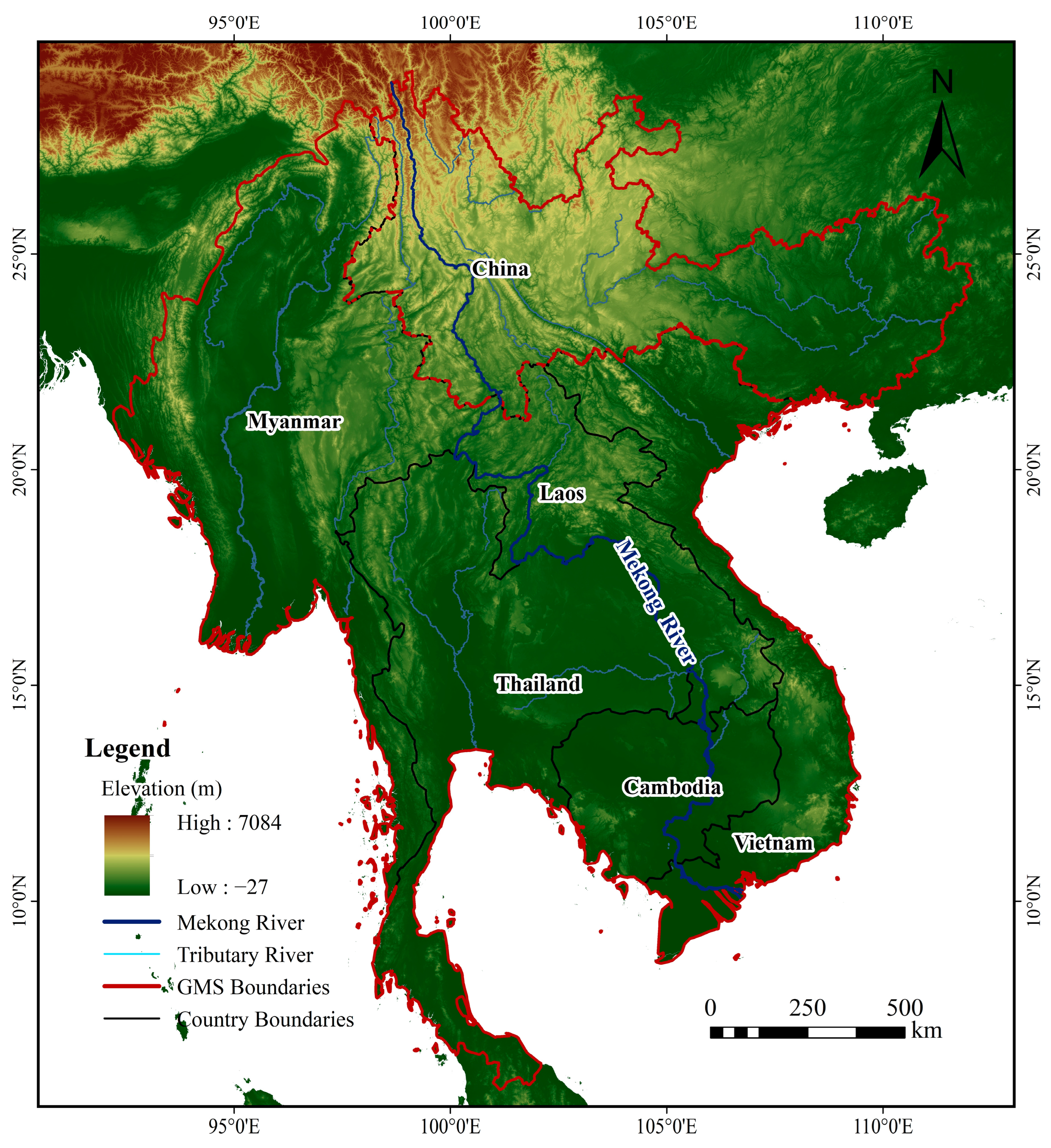
2.1. Study Area

The GMS encompasses regions along the Mekong River, comprising Cambodia, Laos, Myanmar, Thailand, and Vietnam, as well as Yunnan and Guangxi provinces in China. It covers approximately 2.7 million km², with a population of about 378 million [41]. The GMS experiences significant climatic influences, including temperate, tropical, and monsoon climates. The escalating occurrence of extreme weather events poses a substantial threat to the ecosystems of the GMS [42]. The topography of the GMS descends from elevated northern regions to lower southern areas, showcasing diverse geographical features (Figure 1). The GMS boasts substantial tropical forests in Asia, encompassing an expansive forest land of 90.4 million hectares, constituting 48% of the total region in 2010. In the last two decades, vigorous development of GMS’s agriculture has been ongoing, which is primarily attributed to the extensive cultivated area and the impressive output of grains [42,43].

2.2. Assimilation Framework for Various Land-Cover Products

The land cover data assimilation framework (LCDAF) aims to generate the optimal time series of land cover, and it is devoted to minimizing the disparity between the outcomes and the observed data, ensuring alignment with the spatiotemporal evolution of land cover [26]. This study utilizes an assimilation framework to synthesize a time-continuous land cover dataset, synthesizing existing global products. This synthesized dataset harnesses the strengths of various global land cover products, enhancing overall accuracy. The LCDAF comprises observation cost and model cost and defines the comprehensive optimization objective function as:

$$\mathrm{J}\left(\mathrm{x}\right)={\mathrm{J}}^{\mathrm{M}}\left(\mathrm{x}\right)+\mathrm{w}{\mathrm{J}}^{\mathrm{O}}\left(\mathrm{x}\right)$$

(1)

In Equation (1), the land cover time series x is a two-dimensional array determined by time and percentage of area from different land cover types. The model cost and observation cost of a land cover time series are represented by ${\mathrm{J}}^{\mathrm{M}}\left(\mathrm{x}\right)$ and ${\mathrm{J}}^{\mathrm{O}}\left(\mathrm{x}\right)$. w is a weighting factor to determine the degree of influence of observation error relative to model error.

In the LCDAF, the observation cost ${\mathrm{J}}^{\mathrm{O}}\left(\mathrm{x}\right)$ is expressed as the deviation between the estimation x and the individual land cover input. It is defined explicitly in Equation (2) as the weighted mean squared error between the simulated and observed percentages of land cover in the grid:

$${\mathrm{J}}^{\mathrm{O}}(\mathrm{x})={\displaystyle \frac{1}{{\mathrm{N}}_{\mathrm{o}}}}{\sum _{\mathrm{C}}\sum _{\mathrm{o}\mathrm{b}\mathrm{s}}\left({\displaystyle \frac{\mathrm{o}\left(\mathrm{t},\mathrm{C}\right)-\mathrm{x}\left(\mathrm{t},\mathrm{C}\right)}{\mathrm{\epsilon }\left(\mathrm{t},\mathrm{C}\right)}}\right)}^2$$

(2)

where, respectively, $\mathrm{o}\left(\mathrm{t},\mathrm{C}\right)$ and $\mathrm{\epsilon }\left(\mathrm{t},\mathrm{C}\right)$ represent the observed percentage of land cover type C at the time t and its measurement error. The measurement errors are derived from the estimated uncertainties presented in

Table 1. The attribute of global land cover products utilized in LCDAF [26].

Short Name	Legend	Sensor	Spatial Resolution	Time	Estimated Uncertainty
GLCC	IGBP	AVHRR	1 km	1992–1993	30%
GLC2000	FAO LCCS	SPOT4	1 km	2000	40%
UMDLC	Simplified IGBP	AVHRR	1 km	1987	70%
CCI-LC 2000	FAO LCCS	MERIS	300 m	2000	20%
CCI-LC 2005	FAO LCCS	MERIS	300 m	2005	20%
CCI-LC 2010	FAO LCCS	MERIS	300 m	2010	20%
CCI-LC 2012	FAO LCCS	MERIS	300 m	2012	20%
CCI-LC 2015	FAO LCCS	MERIS	300 m	2015	20%
MODIS 2001	IGBP	MODIS	500 m	2001	40%
MODIS 2003	IGBP	MODIS	500 m	2003	40%
MODIS 2005	IGBP	MODIS	500 m	2005	40%
MODIS 2007	IGBP	MODIS	500 m	2007	40%
MODIS 2017	IGBP	MODIS	500 m	2017	40%
MODIS 2019	IGBP	MODIS	500 m	2019	40%

. Higher uncertainty in the observed data reduces the influence of optimization outcomes. $\mathrm{x}\left(\mathrm{t},\mathrm{C}\right)$ denotes the estimated percentage of land cover type C at the time t. $\sum _{\mathrm{C}}$ and $\sum _{\mathrm{o}\mathrm{b}\mathrm{s}}$ represent the sums over all LC types and the available observations, and the ${\mathrm{N}}_{\mathrm{o}}$ represent the number of observations.

While ensuring the minimization of observation error, the derived time series should also align with the inherent pattern of land cover change, implying that the qualitative shift in land cover types takes place gradually over a short period. The linear asymptotic assumption ensures that the model effectively captures and integrates all temporal dynamics from input datasets, thereby minimizing error across various periods. Consequently, the model cost ${\mathrm{J}}^{\mathrm{M}}\left(\mathrm{x}\right)$ is quantified as the variation in each land cover type within this assumption. It is precisely characterized within the assimilation framework as the variance of the first-order difference sequence for different land cover types:

$${\mathrm{J}}^{\mathrm{M}}(\mathrm{x})=\sum _{\mathrm{C}}{\mathrm{\sigma }}^2\left({\mathrm{x}}^{\prime }\left(\mathrm{t},\mathrm{C}\right)\right)=\sum _{\mathrm{C}}\sum _{\mathrm{t}=1}^{{\mathrm{N}}_{\mathrm{t}}-1}{\displaystyle \frac{{\left({\mathrm{x}}^{\prime }\left(\mathrm{t},\mathrm{C}\right)-\overline{{\mathrm{x}}^{\prime }\left(\mathrm{C}\right)}\right)}^2}{{\mathrm{N}}_{\mathrm{t}}-1}}$$

(3)

where ${\mathrm{x}}^{\prime }\left(\mathrm{t},\mathrm{C}\right)$ is the difference of the estimation in land cover type C at the time t from the previous year, ${\mathrm{x}}^{\prime }\left(\mathrm{t},\mathrm{C}\right)=\mathrm{x}\left(\mathrm{t},\mathrm{C}\right)-\mathrm{x}\left(\mathrm{t}-1,\mathrm{C}\right), \mathrm{t}=2,3,\cdots ,{\mathrm{N}}_{\mathrm{t}}$. ${\mathrm{N}}_{\mathrm{t}}$ denotes the total number of timestamps to be solved by the algorithm, and $\overline{{\mathrm{x}}^{\prime }\left(\mathrm{C}\right)}$ denotes the average value computed from the variations at all times. $\mathrm{\sigma }$ is the standard deviation of the difference in the estimation.

Upon the aforementioned equation, the total cost function can be reformulated as the following Equation (4):

$$\mathrm{J}(\mathrm{x})=\sum _{\mathrm{C}}\left[\sum _{\mathrm{t}=1}^{{\mathrm{N}}_{\mathrm{t}}}{\displaystyle \frac{{\left({\mathrm{x}}^{\prime }\left(\mathrm{t},\mathrm{C}\right)-\overline{{\mathrm{x}}^{\prime }\left(\mathrm{t},\mathrm{C}\right)}\right)}^2}{{\mathrm{N}}_{\mathrm{t}}-1}}+\mathrm{w}{\displaystyle \frac{1}{{\mathrm{N}}_{\mathrm{O}}}}\sum _{\mathrm{obs}}{\left({\displaystyle \frac{\mathrm{o}\left(\mathrm{t},\mathrm{C}\right)-\mathrm{x}\left(\mathrm{t},\mathrm{C}\right)}{\mathrm{\epsilon }\left(\mathrm{t},\mathrm{C}\right)}}\right)}^2\right]$$

(4)

When both observation and model costs are minimized, the optimal solution to the overall cost function appears as the land cover time series output, offering a reliable and accurate description of land cover changes over time. Minimizing the cost function constitutes a quadratic programming problem, for which we employed the interior point method to iteratively compute the optimal solution while satisfying the imposed constraints.

Our assimilation framework is configured with a start time of 1980, an end time of 2020, and an interval of 1 year. It utilizes GLCC, GLC2000, UMDLC, CCI-LC, and MCD12Q1 as input data, offering temporal reference for the model spanning from 1987 to 2019 (Table 1). Uncertainty estimates were established to assess the observational errors associated with individual land cover input data in the LCDAF, considering factors such as quality, resolution, and other relevant characteristics. These estimated uncertainties have a marked effect in gauging the relative importance of different input data in the LCDAF. Before synthesizing and processing these land cover products, it is imperative to harmonize their classification systems and spatial resolutions. We employ a simplified 9-class land cover legend from Xu et al. [26] as a reference: water, forest, shrubland, grassland, cropland, wetland, urban, bareland, and snow/ice. The specific conversion relationships between existing classifications and the simplified system are detailed in Xu et al. [26]. The land cover inputs were resampled for the spatial resolution of 1 km under WGS84 geographical reference according to their maximum size. State probability vectors represent the land cover types in each grid to avoid information loss caused by different spatial resampling.

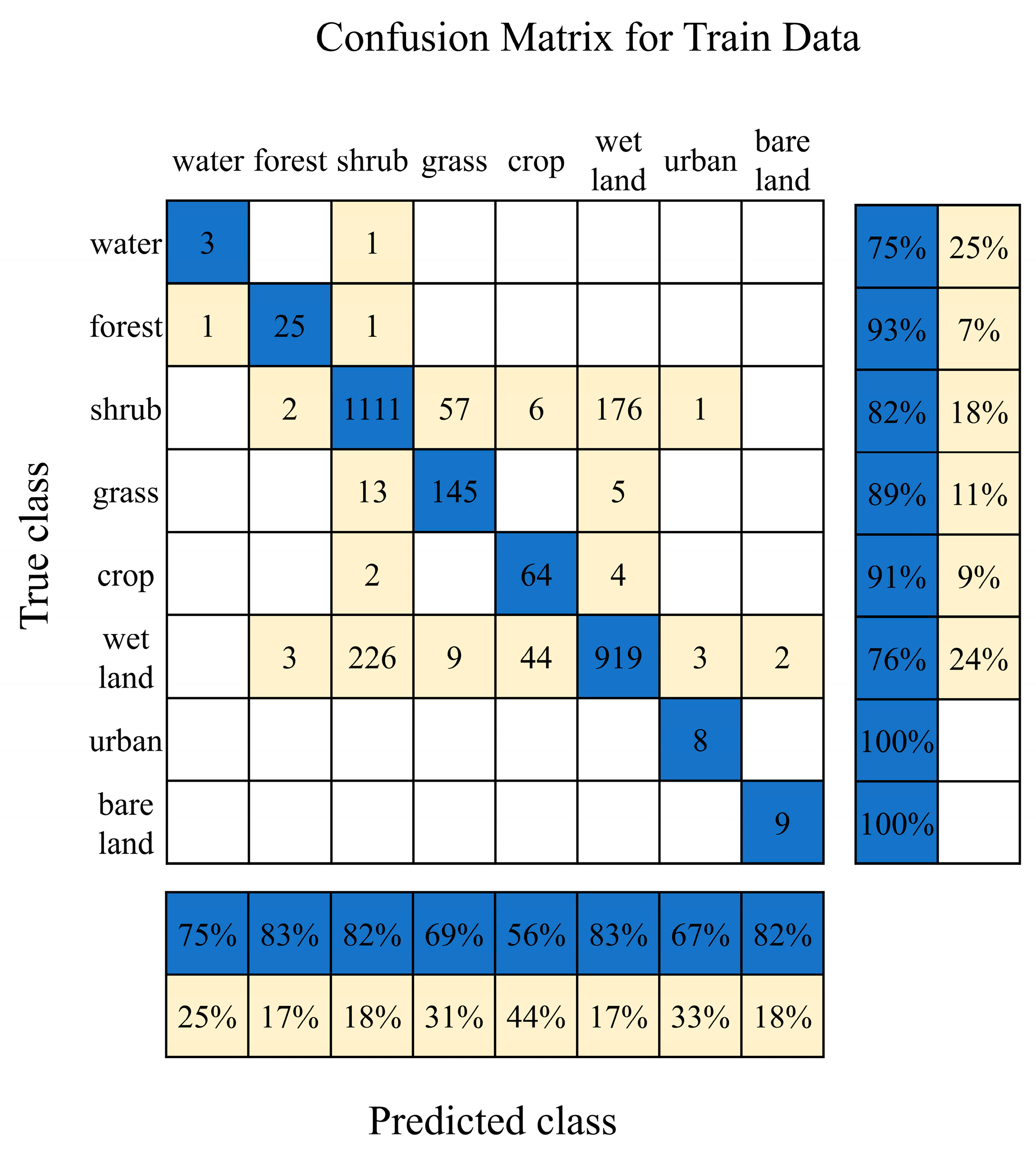
2.3. Accuracy Assessment of Synergetic Land Cover Dataset

For the output series in this study, the period was set longer than the input data, and the results beyond the time range of the input data were utilized as predictions to extend the land cover characteristics within that specific timeframe. Four ground reference datasets cover the period from 2000 to 2013, namely GLC 2000, GlobCover 2005, Terrestrial Ecosystems Parameterization System (STEP), and Visible Infrared Imaging Radiometer Suite (VIIRS) databases, gathered from GOFC-GOLD. These datasets were employed to accurately validate the global results within the input data’s time range. The global reference datasets were transformed into a simplified 9-class land cover legend to ensure consistency with the model outputs.

Given the absence of recent reference data for validating land cover dataset, this study conducted visual interpretation using remotely sensed imagery as an auxiliary for accuracy validation. The MOD09A1 global 500 m surface reflectance product was chosen as a reference, possessing a spatial resolution slightly higher than the model simulations. Subsequently, random points were generated based on cloud-free images in the same period to interpret output results in the GMS. These random points utilized in this study were generated through a stratified sampling technique, ensuring their number met the validation sample size requirements for a specified confidence level, as determined by Equation (5) [44]:

$$\mathrm{n}={\displaystyle \frac{\mathrm{B}\times {\mathrm{\Pi }}_{\mathrm{i}}\times \left(1-{\mathrm{\Pi }}_{\mathrm{i}}\right)}{{\mathrm{b}}_{\mathrm{i}}^2}}$$

(5)

where n represents the theoretical quantity of validation samples that meet the desired confidence level. $\mathrm{B}$ represents the upper percentile of (a/k) × 100th (chi-square distribution with 1 degree of freedom), where a represents the confidence level (0.95 was taken in this study), and k represents the number of land cover types. ${\mathrm{b}}_{\mathrm{i}}$ is the expected precision of the $\mathrm{i}$ category, and ${\mathrm{\Pi }}_{\mathrm{i}}$, is the proportion of area covered by the$\mathrm{i}$category.

The overall accuracy of our synergetic land-cover dataset was assessed through a comprehensive validation of both the samples and corresponding model outputs at different spatiotemporal locations.

2.4. Habitat Quality Evaluation Using the InVEST Model

In this study, we assessed the habitat quality with InVEST 3.14.0 based on a synthesized land cover dataset. InVEST is a modeling system to evaluate ecosystem functioning and provide decision-making support for ecological management and conservation [45]. A distinctive strength of the InVEST model lies in its versatile capacity to handle and simulate ecosystem service functions across extensive regional scales. The InVEST Habitat Quality Module, emerging as a novel tool for appraising habitat quality amidst anthropogenic threats, facilitates the examination of spatial trends in habitat quality driven by land use change. In this model, the formula for calculating habitat quality is as follows [46]:

$${\mathrm{Q}}_{\mathrm{xj}}={\mathrm{H}}_{\mathrm{j}}\left[1-{\displaystyle \frac{{\mathrm{D}}_{\mathrm{xj}}}{{\mathrm{D}}_{\mathrm{xj}}+\mathrm{k}}}\right]$$

(6)

where ${\mathrm{Q}}_{\mathrm{xj}}$ and ${\mathrm{D}}_{\mathrm{xj}}$ respectively, denote habitat quality and habitat degradation degree of land cover type j in the grid x. ${\mathrm{H}}_{\mathrm{j}}$, denotes habitat suitability of land cover type j. k is usually taken to have a value of 0.5 as a fixed constant.

The essential inputs for the module of habitat quality encompass land cover raster, attributes of threat sources, and sensitivity of land cover types. The user manual can provide detailed guidance on requirements and methodologies [40,47]. The basic setting of model parameters refers to the model manual and previous research. The model parameters were adjusted to align with the input data’s characteristics and the study area’s specific attributes. Over the past few decades, the GMS has been significantly impacted by urban development and agricultural activities, which are the primary threat to its habitats. Construction land can pressure the ecosystems through development projects, including built-up areas, road transportation networks, and rural residential zones. Reference values of threat weight for these types of construction land typically range from 0.6 to 1, reflecting varying degrees of ecological impact. Due to the land cover classification system employed in this study, which encompasses all forms of construction land, an average value is calculated and used as the weighting factor. The cropland, a blend of semi-artificial landscapes, poses a comparatively milder threat to natural ecosystems than construction land. Therefore, a lower weight of 0.6 is assigned to cropland.

Table 2. The relative attributes of the threat source.

Threat Factors	Maximum Threat Distance (km)	Weight	Spatial Decay Type
Cropland	4	0.6	exponential
Urban	8	0.8	exponential

provides attributes associated with these factors.

Habitat suitability and sensitivity exhibit significant variation typically within the [0, 1] range, and the specific settings refer to the model’s default values and other relevant literature (

Table 3. Sensitivity of different land cover types to threat source.

Land Cover Type	Habitat Adaptability	Cropland	Urban
Water	0.9	0.7	0.9
Forest	1	0.6	0.8
Shrubland	0.9	0.5	0.6
Grassland	0.8	0.3	0.5
Cropland	0.5	0.2	0.5
Wetland	1	0.6	0.9
Urban	0	0	0
Bareland	0.1	0.1	0.1
Snow/Ice	0	0	0

). Forests and wetlands are the main habitats for important species, with a habitat suitability of typically 1. For other habitat types, the simple systems with artificial transformation have poor habitat suitability [48]. Therefore, the habitat suitability for shrubland and water bodies is 0.9, grassland is 0.8, and crops are 0.5. According to the principles of biodiversity conservation in landscape ecology, land covered with lower natural degrees is less sensitive to disturbance; thus, completely artificial systems almost lose habitat sensitivity [49,50].

2.5. Landscape Pattern Indicators Derived from Land-Cover Change

Frequent anthropogenic activities affect land use patterns and simultaneously threaten habitat quality. Land use intensity and landscape fragmentation can be proxy indicators of anthropogenic interference. Consequently, we focused on these two indicators to assess their relationship with the spatial distribution of habitat quality. This analysis aims to elucidate the drivers behind variations in habitat quality.

Land use intensity (LUI) is an indicator for measuring the ecological naturalness within a specific region, considering the distinct land cover characteristics. Based on its inherent attributes, land cover is categorized into four intensity types: bare land, ecological land (forest, grassland, shrubland, watershed, and wetland), agricultural land, and urban land. Each category is assigned an intensity grade ranging from 1 to 4. Precisely, LUI is calculated as follows in Equation (7)

$$\mathrm{L}=\sum _{\mathrm{i}=1}^{\mathrm{n}}{\mathrm{A}}_{\mathrm{i}}{\displaystyle \frac{{\mathrm{C}}_{\mathrm{i}}}{\mathrm{C}}}$$

(7)

In the Equation (7), ${\mathrm{A}}_{\mathrm{i}}$ represents the intensity grading index of level $\mathrm{i}$ in the region. C and ${\mathrm{C}}_{\mathrm{i}}$ represent the total area and part of the region. n is the number of intensity grading on land use.

Landscape fragmentation assesses the degree of segmentation in the landscape based on the number of fragments, size, shape, and continuity. In this analysis, we computed two key indexes, including patch density and edge density with FragStats 4.2, to characterize the landscape fragmentation of the region. FragStats (Fragment Statistic) is a software tool that analyzes the spatial distribution patterns of land cover classification maps. It includes modules for calculating over 100 landscape indices. Patch density (PD) reflects the number of patches per area, providing insights into the degree of segmentation and relative connectivity of different land cover types. Edge density (ED) is measured as the length of edges between adjacent heterogeneous patches per area, offering additional perspectives on landscape fragmentation. The two indices are calculated as follows in Equations (8) and (9) [51]:

$$\mathrm{PD}={\displaystyle \frac{\mathrm{N}}{\mathrm{A}}}$$

(8)

where N is the total number of patches in the landscape, and A is the total area of the landscape (m²).

$$\mathrm{ED}={\displaystyle \frac{\mathrm{P}}{\mathrm{A}}}$$

(9)

$\mathrm{P}$ is the length of the edge in the landscape, and A refers to the formula above.

3. Results

3.1. Global and Regional Validation Results

The overall validation accuracies for the various land cover products are expressed by the average accuracies across all validation points in the reference datasets over different temporal intervals, as detailed in

Table 4. Validation results using diverse reference data across various periods.

Products		Accuracy (%)
		Global (2000–2013)					GMS (2020)
Time	Name	GLC2000ref	GlobCover 2005ref	STEP	VIIRS	Average	Random Samples
1980–2020	LCDAF	67.2	79.0	78.6	70.9	73.9	80.4
2000	GLC2000	61	/	59.1	55.1	58.4	/
2000–2015	CCI_LC	58.4	76.7	64.7	60.3	65.0	/
2001–2019	MODIS_LC	65	76.3	79.6	71.3	73.1	/

.

In the overall assessment, the synthesized time series exhibited a remarkable accuracy of 73.9%, notably higher than the average accuracy of other input data. The MODIS_LC dataset outperforms our product in accuracy when evaluated against the STEP and VIIRS datasets. This performance of MODIS_LC can be attributed to its calibration using these two datasets as references, which naturally enhances their accuracies. However, their comparative advantage over our product diminished when the additional datasets (those not used as references by MODIS_LC) were evaluated. The validation results for the GLC2000ref and GlobCover2005 datasets show that our product outperforms both GLC2000 and CCI_LC. Notably, GLC2000, when referenced against GLC2000ref, still falls short of the accuracy achieved by our product when evaluated with GLC2000ref. This compelling evidence suggests that the LCDAF adeptly assimilates the characteristics of diverse input data, producing a coherent land cover time series with superior classification results compared to individual land cover products.

Moreover, the accuracy of 80.4% obtained from the random point sample set precisely for the GMS in 2020 underscores two pivotal aspects. Firstly, our product exhibits great accuracy at a regional scale, offering precise foundational data for subsequent regional analyses and investigations. Secondly, the assimilation framework employed in this study showcases predictive capabilities by extending land cover characteristics beyond the temporal scope of the input data. Figure 2 shows the confusion matrix of real and predicted categories, as well as the accuracies of all categories. Overall, short vegetation such as shrubland, grassland, and cropland are prone to misclassification. Due to their similarity in features such as texture and spectrum, these classification errors may coexist in the input data. By the confusion matrix, indices such as precision and recall were calculated simultaneously, as shown in

Table 5. Indicators of classification performance from confusion matrix.

Indicator	Water	Forest	Shrub	Grass	Crop	Wetland	Urban	Bareland
Precision	0.75	0.83	0.82	0.69	0.56	0.883	0.67	0.82
Recall	0.75	0.93	0.82	0.89	0.91	0.76	1.00	1.00

. The precision shows that the correct classification of forests, shrubs, and wetlands is relatively significant. Due to the uneven number of random samples, the precision cannot fully reflect the classification performance of the model. Except for water bodies, the recall rates of other land cover categories are relatively high. This indicates that the LCDAF has superior performance and can greatly reduce the model’s false positive predictions.

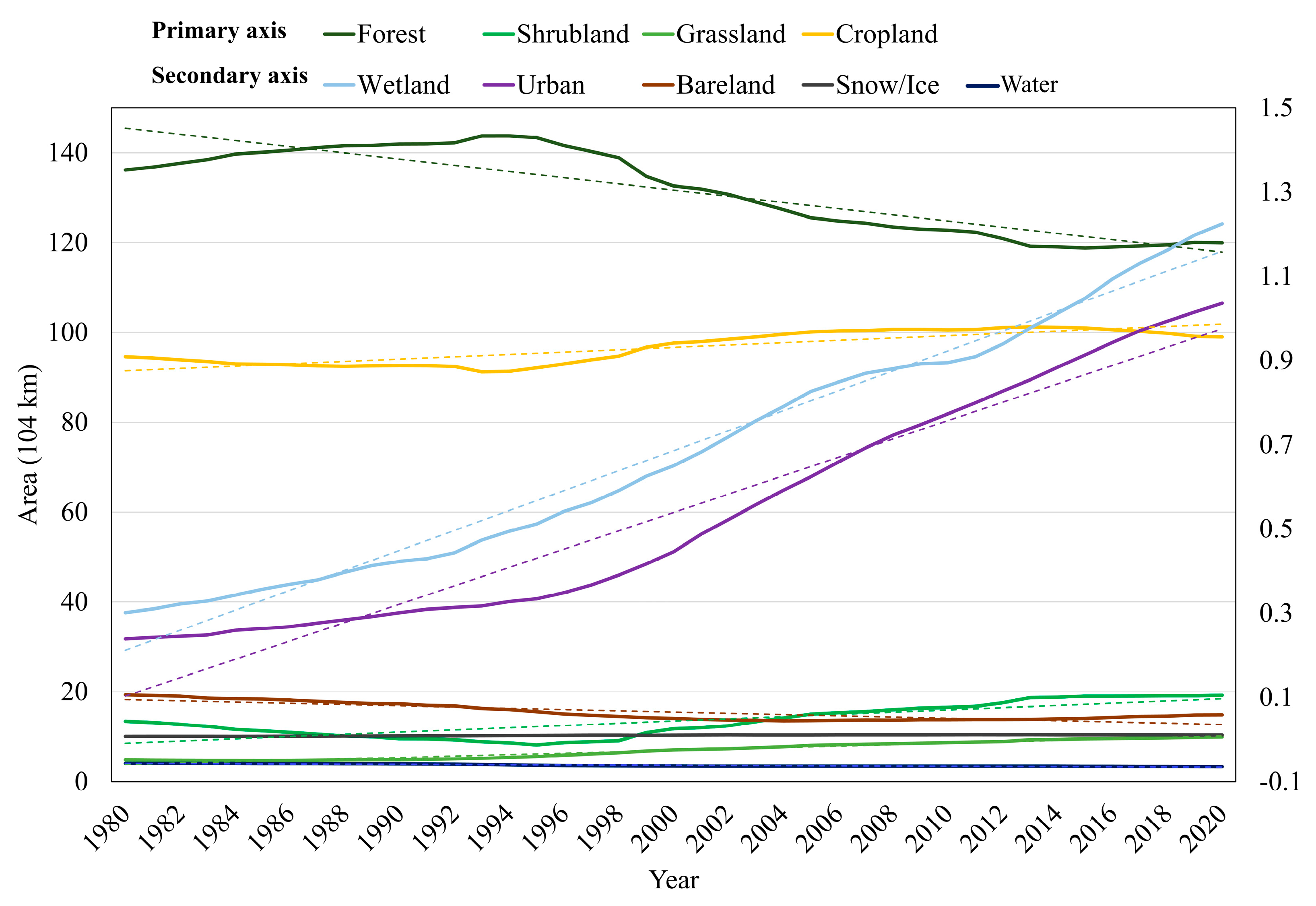
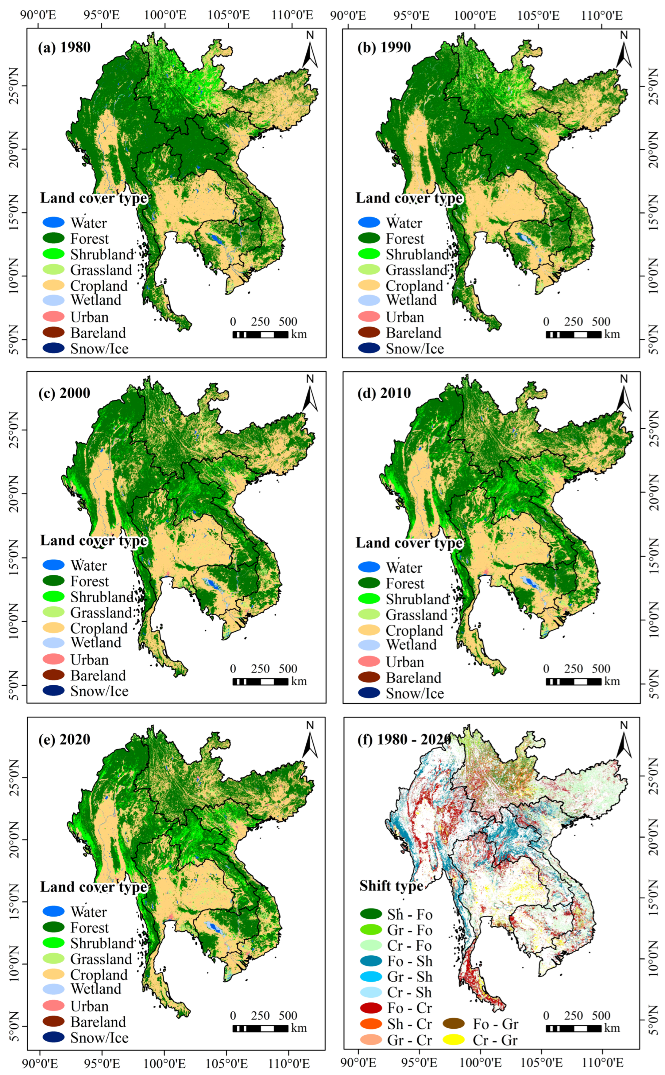
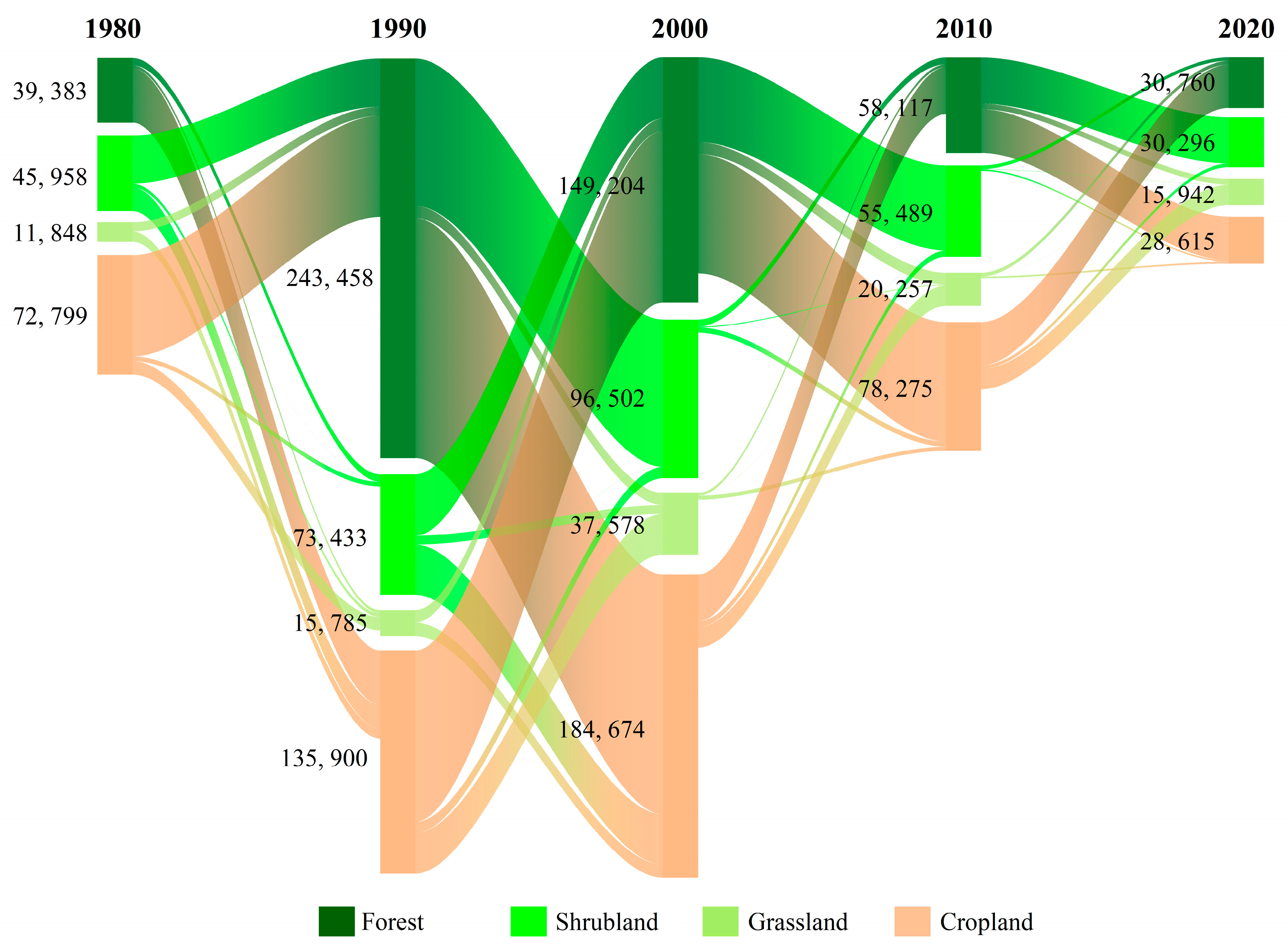
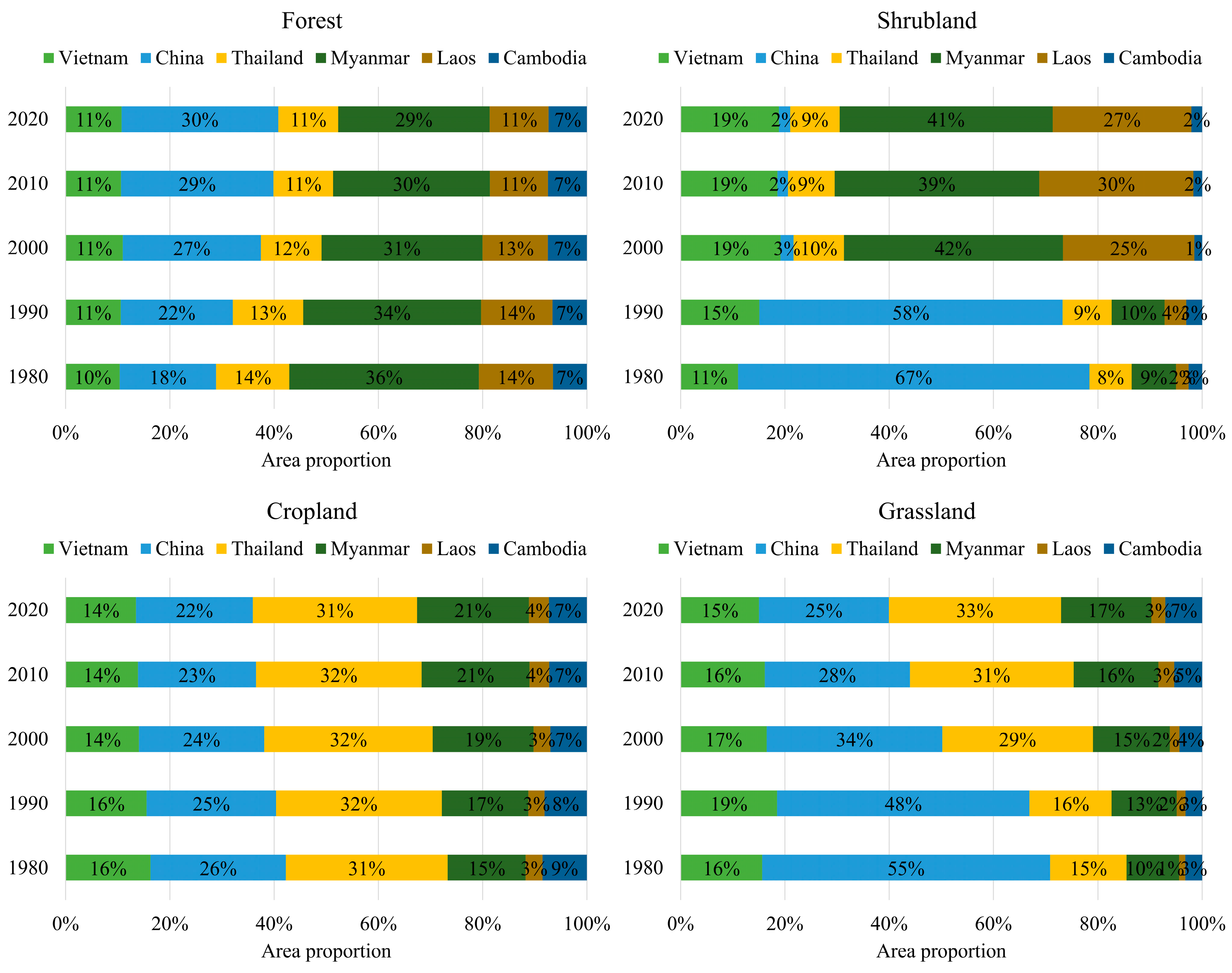
3.2. Dynamic Characteristics of Land Cover

Across the GMS, all land cover types display distinct trends from 1980 to 2020. Croplad, grassland, shrubland, urban areas, and wetlands have experienced consistent growth, while forests, barelands, and water show a declining pattern (Figure 3). In 2020, forests, cropland, shrubland, and grassland emerged as the predominant parts, comprising approximately 47%, 39%, 8%, and 4% of the region’s total area.

The two predominant land cover types, forest and cropland, exhibit extensive distribution across the various countries and regions within the GMS. Forest land, as the primary land cover type, witnessed an expansion until 1995, notably in Guangxi Province, China. After 1995, there was a contraction, resulting in a total area of 1,199,209 km² by 2020. In contrast, cropland experienced a decline in total area before 1995, followed by a subsequent increase. Overall, cropland area in 2020 rose by 5% compared to 1980, primarily attributed to forest encroachment and wasteland reclamation [52]. Shrubland in Yunnan Province of China notably decreased until 1995 (Figure 4). However, extensive shrubland emergence in Myanmar, Laos, and Vietnam led to an overall increase in the GMS. Fragmented grasslands, often adjacent to forests and croplands, expanded by 51,318 km² within the study period (Figure 5). Urbanization exhibited a remarkable acceleration, fourfold in urban areas, to reach 10,360 km² by 2020. Concurrently, bareland areas are nearly halved, predominantly in coastal zones. With increasing human activities, water area decreased by 7106 km² over four decades. However, nearby wetland areas, especially around Tonle Sap Lake of Cambodia, exhibited a corresponding increase.

The landscape pattern of the GMS underwent significant conversions from 1980 to 2020, with more than 60% of the total area. As outlined in

Table 6. Area of land cover conversions (km²) from 1980–2020.

Land Cover		1980
		Water	Forest	Shrubland	Grassland	Cropland	Wetland	Urban	Bareland	Snow/Ice
2020	Water	19,432	2207	917	733	9313	80	41	307	0
	Forest	5035	891,037	69,954	14,586	217,668	842	42	44	0
	Shrubland	393	171,361	4695	115	15,599	0	9	0	0
	Grassland	1644	18,339	7965	15,561	55,177	42	40	413	41
	Cropland	11,779	274,024	49,750	16,059	636,775	226	1016	165	0
	Wetland	1378	4419	288	340	3947	1819	0	55	0
	Urban	405	362	627	423	7300	1	1239	2	0
	Bareland	69	27	117	68	242	0	0	55	8
	Snow/Ice	0	0	41	18	6	0	0	17	21

, these transformations were predominantly observed in forest, shrubland, grassland, and cropland, with the most extensive conversions within the GMS taking place between shrubland and cropland. A significant 20% of forested land, covering an area of 274,024 km², underwent conversion to cropland across various countries and regions within the GMS. Conversely, 23% of cropland, predominantly situated in China, Vietnam, and Cambodia, underwent reforestation. Furthermore, from cropland to reforestation, substantial grassland areas were converted from cropland in various countries and regions, totaling 55,177 km², primarily in Thailand. Concurrently, significant conversions occurred between forest and shrubland. Shrubland-to-forest conversion accounted for 69,954 km², mainly observed in Yunnan Province, China.

In contrast, forest-to-shrubland conversion was mainly observed in Myanmar and Laos, covering 171,361 km². Figure 6 depicts the significant changes in land cover over the last four decades, with the most pronounced alterations occurring between 1990 and 2000. During this period, substantial conversions occurred in forest, shrubland, grassland, and cropland, amounting to approximately 243,458, 73,433, 15,785, and 135,900 km², respectively. This decade coincided with the initiation of GMS cooperation, which marked significant changes in the region’s social development and land use.

Throughout the study period, each country and region within the GMS experienced unique alterations in land cover. In the provinces of Yunnan and Guangxi, China, forested land exhibited consistent expansion from 1980 to 2020, albeit at a diminishing rate (Figure 4). This growth chiefly lies in converting forest from grassland, shrubland, and cropland, ultimately constituting 30% of the total forested land in the GMS by 2020 (Figure 7). The increase in forested areas and the decline in agricultural land in these provinces can be attributed to the afforestation policies enacted by the Chinese government since 2000 [53,54,55,56]. Conversely, Thailand, Myanmar, and Laos witnessed a consistent decline in forested land cover over the specified period. Vietnam and Cambodia initially saw an upswing in forest cover, which was subsequently followed by a decrease. Cambodia, in particular, has witnessed a substantial loss of approximately 18% of its forest area since 2000, primarily attributed to extensive land acquisition practices [41,57,58]. Vietnam’s forest loss rate has achieved stability over the past decade, attributed to successful replanting programs and reforestation efforts [27]. Myanmar and Laos witnessed substantial conversion of forest land to shrubland, notably between 1990 and 2000, with rates surpassing a fourfold increase. FAO reports underscore the alarming extent of forest loss in these nations from 1990 to 2010 [27].

In Laos, the expanse of shrubland experienced a remarkable surge, escalating from 3239 km² in 1980 to 50,049 km² by 2020. Simultaneously, there was a significant reduction in shrubland within Yunnan Province, China, causing the shrubland area share in the GMS to plummet from 67% in 1980 to a mere 2% by 2020 (Figure 7). Grassland in the GMS, excluding China, demonstrated a consistent upward trajectory in the area across all periods, with the most substantial increase observed between 1990 and 2000. Thailand, Myanmar, and Laos exhibited an overall growing trend in cropland areas, with Myanmar registering the swiftest rate at approximately 50% between 1980 and 2020 (Figure 4). In contrast, Vietnam, China, and Cambodia witnessed variations in cropland areas, resulting in an overall decline of approximately 10%. Despite this, the proportion of cropland in the GMS increased throughout the study period. Notably, China’s Yunnan and Guangxi provinces held a dominant 55% share in 1980, gradually giving way to Thailand, which claimed a 33% share by 2020 (Figure 7).

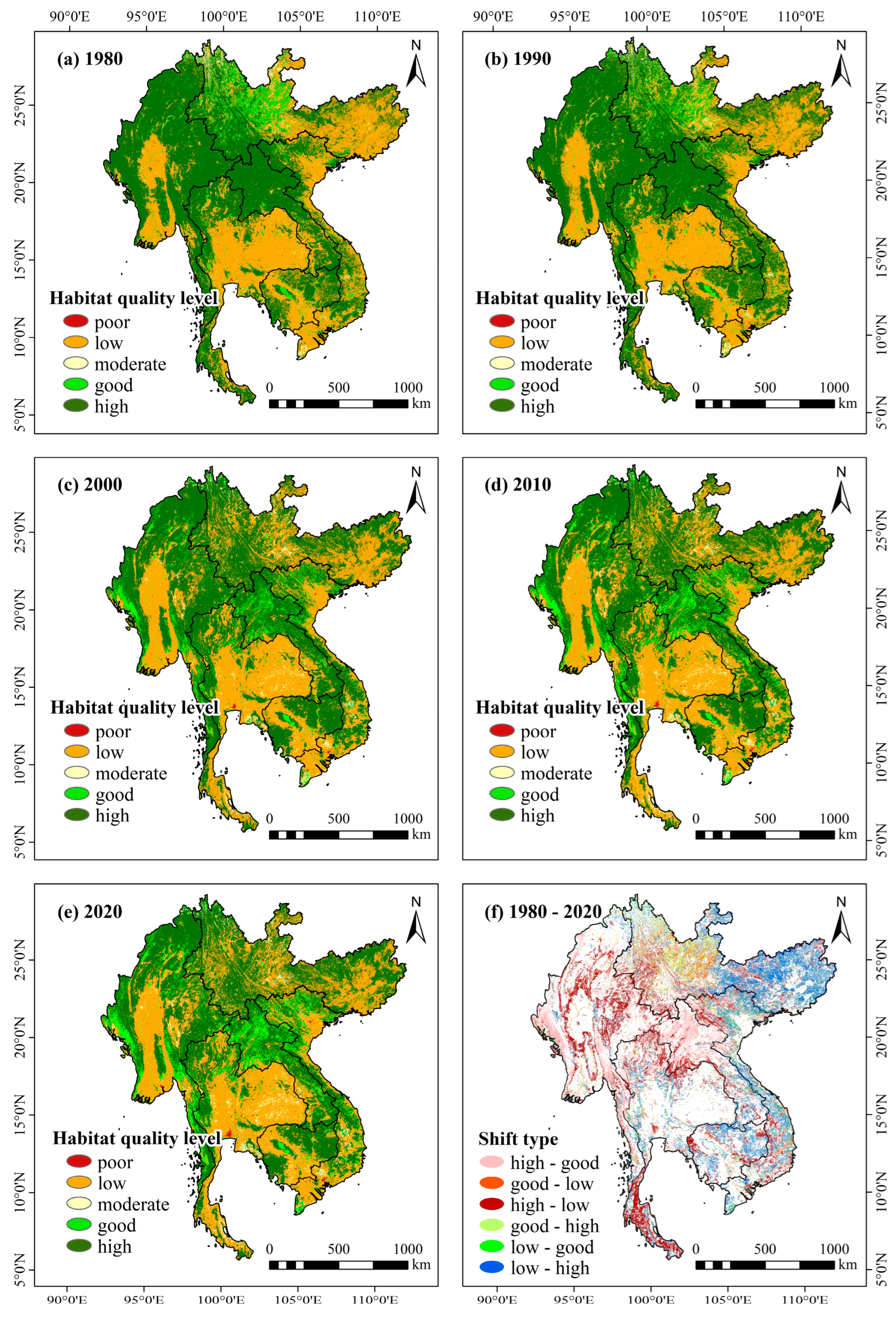
3.3. Dynamic Characteristics of Habitat Quality

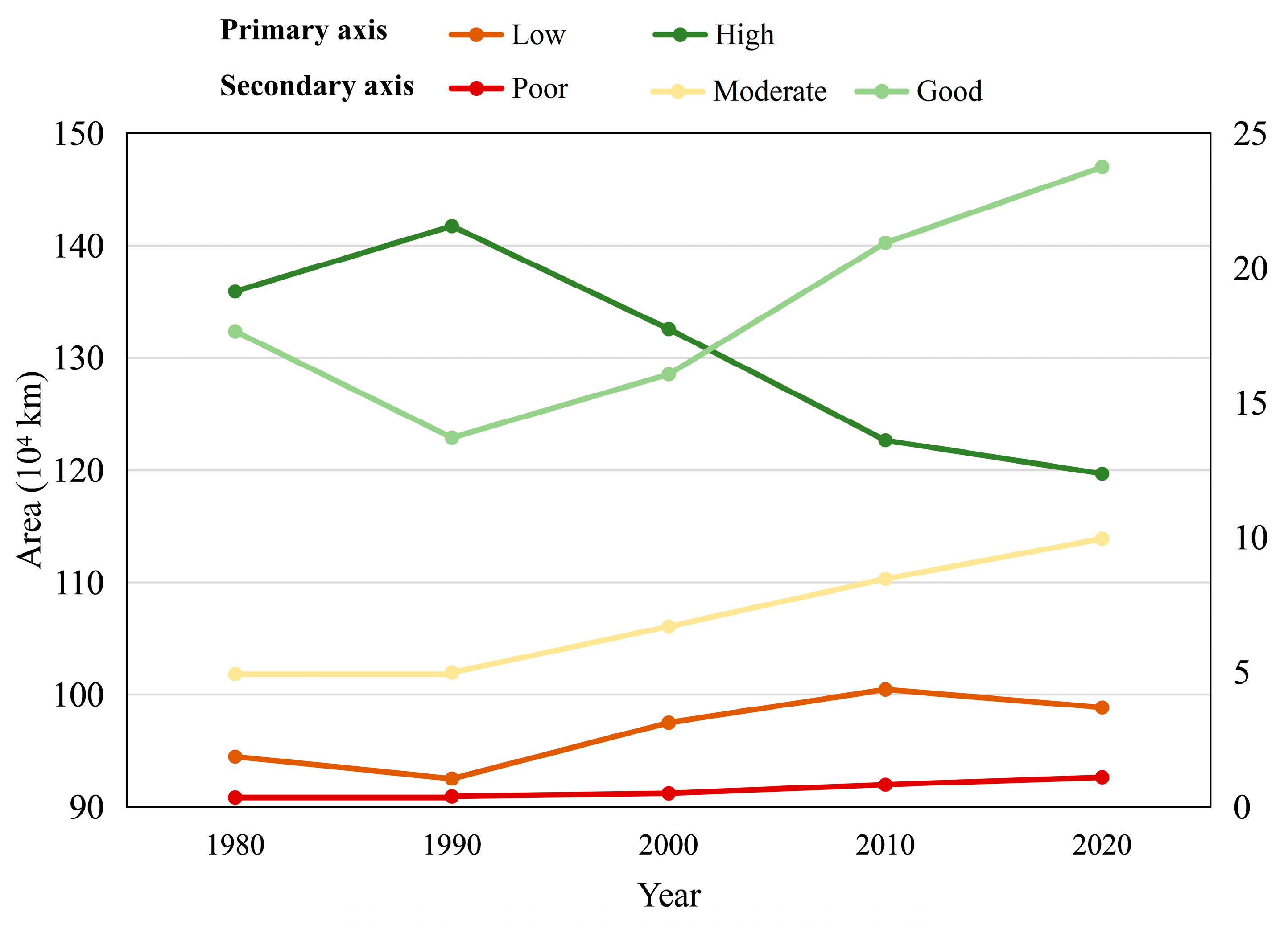
3.3.1. Habitat Quality Grades

The habitat quality of the GMS consistently held a moderate level, as indicated by mean values across the region: 0.794, 0.799, 0.787, 0.776, and 0.775 for the years 1980, 1990, 2000, 2010, and 2020, respectively (Figure 8). This trend suggests a modest overall decline of 2.4%. The depiction of habitat quality distribution in Figure 8 reveals substantial spatial variation. High-quality regions were predominantly northwest, with concentrated forest, shrubland, and wetland areas. Conversely, areas with lower habitat values were dispersed across regions marked by intensive cropland and urban development. Noteworthy improvement in habitat quality was observed in central Thailand and the eastern part of the GMS. While areas experiencing a decline in habitat quality were predominantly located in the northwestern GMS and the southern islands of Thailand. Despite an overall decrease in habitat quality after 2000, high-value areas have a discernible enhancement.

The raster data of habitat quality in the GMS spanning from 1980 to 2020 were classified into five categories with a natural breakpoint method: poor (0–0.3), low (0.3–0.6), moderate (0.6–0.8), good (0.8–0.9), and high (0.9–1). Figure 9 shows that the regions characterized by high-grade habitat quality comprised approximately a significant % of the study area, encompassing approximately 50%. These two categories collectively encompass around 90% of the study region and low-grade habitat quality (Figure 10). The high-grade habitat quality areas displayed a pattern of increase and subsequently decrease from 1980 to 2020, resulting in an overall reduction of 12%. Most of these areas experiencing degradation transitioned into both good and poor grades, predominantly situated in the west-central GMS and the southern islands of Thailand, encompassing specific areas of 176,297 and 271,756 km², respectively (

Table 7. Area of conversions (km²) for habitat quality from 1980 to 2020.

Habitat Quality		1980
		Poor	Low	Moderate	Good	High
2020	Poor	1343	7547	1097	822	2405
	Low	1181	636,796	18,030	62,067	271,756
	Moderate	281	57,490	12,386	10,441	19,117
	Good	599	28,944	4456	27,486	176,297
	High	112	215,248	13,434	75,934	893,617

).

In contrast, the area covered by the remaining classes of habitat quality exhibited an ascending trend, with the low and moderate categories experiencing the most rapid expansion by more than one factor. Noteworthy transitions from low to high-quality habitat were predominantly observed in the Guangxi Province of China, Cambodia, and central Vietnam, covering approximately 215,248 km². Despite these large areas showing improved habitat quality, these changes did not elevate the average habitat level across the entire GMS.

We assessed the mean habitat quality values for each country and region within the GMS over various intervals from 1980 to 2020, as illustrated in Figure 11. Laos exhibited the highest habitat quality, with average indices ranging from 0.888 to 0.931. This consistently superior habitat quality throughout the study period can be attributed to Laos’s relatively small cropland area. However, the notable conversion of forested to shrubland in northern Laos after 1990 reduced habitat quality, as our model deemed shrubland less suitable than forested land. Myanmar witnessed a noteworthy decline in habitat quality attributed to substantial forest losses, particularly between 1990 and 2000.

Nevertheless, it succeeded in maintaining a relatively high habitat quality. Vietnam, Cambodia, and the two Chinese provinces exhibited moderate-level habitat quality, all undergoing an increase and subsequently decreasing around the year 2000. This pattern aligns with contemporaneous trends in changes to forest land. Thailand recorded the lowest habitat quality in the region, with average indices ranging between 0.663 and 0.699, significantly below the GMS average. The extensive cropland in Thailand, heavily affected by human activities, contributed substantially to its low habitat suitability. From 1990 to 2000, a substantial portion of the forest in Thailand’s northern islands underwent conversion to grassland and cropland, resulting in a 3% drop in habitat quality. Subsequently, Thailand’s habitat quality remained relatively stable, hovering around 0.67. Between 2010 and 2020, there were minimal changes in land use patterns across the GMS, resulting in no significant fluctuations in habitat quality across the various countries and regions. This phase of relative stability in land cover implies a period of ecological equilibrium, albeit at varying levels of habitat quality across the GMS.

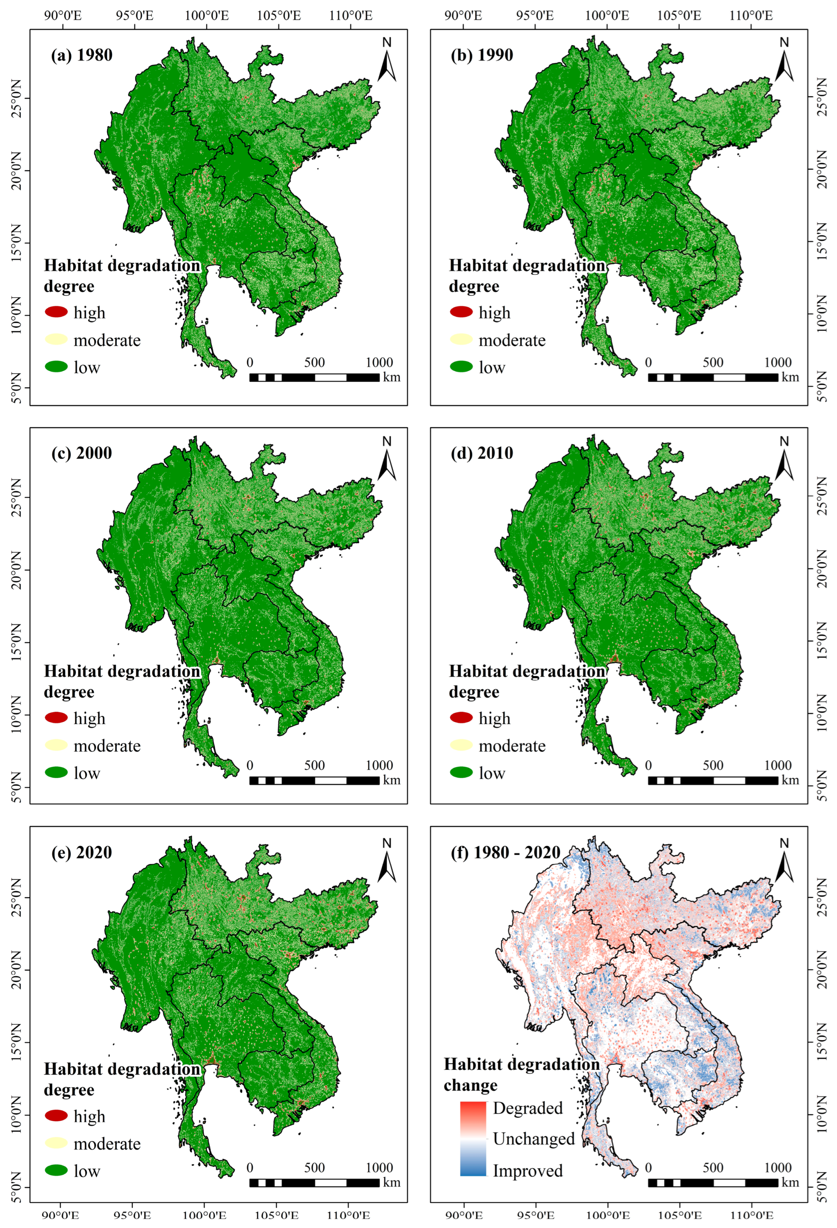
3.3.2. Habitat Degradation Degree

Over the research period, the extent of habitat degradation in the GMS exhibited a generally increasing trend. The habitat degradation degree was classified into three categories with the natural breakpoint method: low (0–0.1), moderate (0.1–0.2), and high (0.2–0.5). The results of habitat degradation grading in GMS from 1980 to 2020 are depicted in Figure 12. Most areas exhibited low-grade habitat degradation, while urban regions heavily impacted by human activities demonstrated a high grade. This degradation tends to diminish with increasing distance from urban centers, especially in highland and mountainous areas less affected by human influence. Notably, regions characterized by a single land cover type also demonstrated a lower degree of habitat degradation. Land cover conversions contribute to increased fragmentation, heightening the risk of habitat degradation. Significant changes in land cover across the GMS led to an overall increase in habitat degradation from 1980 to 2020, particularly notable in the central part of the GMS. This area witnessed frequent conversions among forest, cropland, shrubland, and grassland. The convergence of four national borders, highly dynamic land cover changes, and well-developed water systems made this region susceptible to human disturbances. Despite an overall decrease in the total forest area in Cambodia, the improvement in forest fragmentation in the southwest and northeast helped alleviate habitat degradation in these regions. In Guangxi Province, China, the policy of converting farmland back to forests had a positive impact on mitigating habitat degradation, underscoring the effectiveness of targeted environmental policies in reducing ecological impacts.

3.4. Landscape Change Effects on Habitat Quality

The habitat quality within the watershed is notably influenced by the development of human society, with LUI emerging as a primary determinant. Habitat quality of the GMS has generally declined with the intensification of land use (Figure 11). The widespread expansion of intensive agriculture, encroaching upon natural areas, stands out as a primary contributor to this prevailing trend. Regionally, Vietnam, Cambodia, and the two Chinese provinces exhibited a decrease in LUI, aligning with concurrent improvements in habitat quality over the same period. In contrast, Thailand, Myanmar, and Laos exhibited an opposing trend, marked by increasing LUI and declining habitat quality. Employing Pearson’s correlation analysis, we discerned a significantly negative correlation of −0.97 (p < 0.01) between LUI and the habitat quality index. The negative correlation suggests that regions experiencing intensified human activities pose high-intensity land development and more significant habitat threats. This finding aligns with the core concepts in the computational modeling of habitat quality. LUI can characterize habitat quality from the perspective of landscape patterns on a large scale.

In Section 3.3.2, we mentioned a connection between the fragmentation of land use patterns and the degree of habitat degradation at more minor spatial scales. Patch and edge densities generally increased in the GMS, with Myanmar and Laos exhibiting the fastest rates of fragmentation and corresponding habitat degradation (Figure 11). PD and ED, as indicators of landscape fragmentation, showed a negative correlation of −0.62 and −0.73 (p < 0.01) with habitat degradation. Landscape fragmentation disrupts the ecological integrity of supporting habitats, further threatening the habitat quality of the region. Areas with a high degree of habitat degradation were prominently observed in natural and semi-natural regions characterized by elevated levels of fragmentation (Figure 12). It also suggests that landscape fragmentation impacts the degree of habitat degradation at localized scales and the effect of LUI. Diverse ecological protection measures, including reforestation and afforestation projects, mitigate landscape fragmentation and LUI, positively affecting the quality of the environmental environment [59,60]. These findings underscore the significance of integrating effective land use management and ecological restoration strategies to uphold and enhance habitat quality, especially in regions undergoing rapid socio-economic changes.

4. Discussion

4.1. Strengths and Limitations of the Assimilation Framework

The time-continuous land cover sequence generated by LCDAF exhibits the highest overall accuracy, benefiting from integrating input data characteristics. However, this accuracy manifests variably across different time nodes. Notably, the validation accuracy and improvement relative to the input data for the year 2000 were markedly lower than in later periods. The low uncertainty inherent in the GLC2000 and CCI-LC2000 datasets bolsters the reliability of the fusion outcomes. Therefore, the density and quality of input data affect the fusion effect.

Due to the scarcity of observation data before 2000, the assimilation framework relied more on UMDLC and GLCC. Despite the high uncertainty of these two data, the assimilation framework can only refer to them during this period. Compared to UMDLC and GLCC, GLC2000 and CCI-LC2000 show the conversion from shrubland to forest in two provinces of China and the conversion from forest to shrubland in Laos and Myanmar from 1987 to 2000. The optimization results of the assimilation framework are consistent with the overall trend of changes from observed data. The land cover conversions in GLC2000 that do not conform to actual changes have been reduced through the fusion method. This indicates one of the advantages of our assimilation framework: the technique can still work in the absence of input data to produce land cover results maximally consistent with observed data. From 2000 onward, the data input frequency increased to once every one or two years, markedly reducing errors associated with linear assumptions within the model. This enhancement in data input frequency bolsters current accuracy and extends predictively beyond the input timeframe. Moreover, with abundant observational data, we strategically input data into the model staggered over time to diminish the dominance of any single dataset on the fusion results. Although lower data density might constrain the improvement potential of the fusion product, our model is adept at compensating for gaps caused by missing observational data. The LCDAF offers significant advantages over traditional image classification methods based on remote sensing data, particularly its ability to mitigate noise in adverse weather conditions. This capability ensures more robust and reliable land cover assessments across diverse temporal and environmental contexts.

The accuracies of large-scale land cover products often demonstrate pronounced regional discrepancies, which are typically attributed to considerable differences in classification methodologies and data quality. The fusion of these products in LCDAF enhances the classification results performance in the region. To further evaluate the regional results’ accuracy and consistency, we also selected the GLC-FCS data with a long period and early traceability for comparison [61]. Overall, GLC-FCS exhibits better average accuracy in the GMS region with a high spatial resolution of 30m (

Table 8. Regional validation results using diverse reference data across various periods.

Products		Accuracy (%)
Time	Name	GLC2000 ref	GlobCover 2005ref	STEP	VIIRS	Average
1980–2020	LCDAF	44.4	83.3	50.0	75.7	63.4
1985–2020	GLC-FCS	55.6	66.7	70.8	74.2	66.8

). However, the validation results of GlobOver2005ref and VIIRS showed significant superiority of LCDAF. Although the spatial resolution of our fusion product is much lower than that of GLC-FCS, the spatial distribution and variation trends of the two are consistent. This is reflected in more detailed cases of three representative regions of GMS in Section 4.3. Our global fusion efforts have already yielded satisfactory outcomes in regional validations, and these are poised for further enhancement through models based on regional observational data. Currently, the operational demands of running LCDAF with a spatial resolution of 1 km are considerably high in terms of time and computational resources. We plan to refine the model structure and enhance assimilation efficiency. Such improvements will enable LCDAF to incorporate higher spatial resolution data and a broader array of observational inputs. This strategic enhancement will be pivotal in minimizing errors and delivering high-precision land cover fusion products, thus advancing our capacity to provide detailed and accurate environmental assessments on a global and regional scale.

4.2. Uncertainties of Habitat Quality Model

Implementing the InVEST model has demonstrated its efficacy in assessing habitat quality nationally [62]. While the assimilation framework employed in our study helps reduce errors in land cover data, the synergetic dataset still introduces certain uncertainties in producing habitat datasets. These uncertainties primarily arise from land cover datasets’ classification scheme and spatial resolution. A lower spatial resolution can obscure the variability of habitat types in model outputs. Pixels characterized by high urban coverage typically indicate lower habitat quality within the model. However, studies such as those by Kowarik [62] and Pesola et al. [63] suggest that biodiversity levels in urban areas can be unexpectedly high. Likewise, extensive vegetated areas may overlook potential threats to ecosystems posed by interspersed residential zones and infrastructures like roadways, which are not adequately captured because of the coarse resolution of the data. Moreover, oversimplifying the classification system tends to homogenize the complexity of different habitats, reducing their sensitivity and consequently dampening the representation of the high heterogeneity characteristic of the GMS’s natural environment. Future improvements in habitat quality assessment can be achieved by updating input data from assimilation frameworks by employing more sophisticated classification systems and higher spatial resolution.

The lack of field observation data limits our ability to fully account for variations in biodiversity and habitat quality parameters across large spatial extents. The approach, grounded in expert knowledge, involves assessing habitat quality parameters in different regions based on professionals’ experiences in ecological conservation and urban planning. We performed systematic and quantitative sensitivity analysis to evaluate uncertainty in the InVEST model’s habitat quality outputs. Owing to the model’s inherent complexity involving numerous land cover types and interconnected parameters, our experimental design prioritized cropland-related variables through targeted sensitivity testing. This strategic selection was grounded in cropland’s dual role as both the threat source and primary land cover category within the study area. Our methodological framework involved parametric perturbation of four key attributes: threat distance, threat weight, habitat suitability, and habitat sensitivity, with systematic ±50% variation from baseline values. The resultant uncertainty analysis revealed differential parameter robustness, with habitat suitability demonstrating comparatively ±15% (Figure 13). This elevated sensitivity emerges from habitat suitability’s fundamental role in determining habitat quality estimations. At such a large spatial scale of analysis, this magnitude of uncertainty remains operationally acceptable for habitat quality assessment. Integrating expert opinions with the InVEST model mitigates the uncertainty inherent in habitat quality assessments. However, this approach demands extensive, continuous, and multifaceted engagement, and the historical on-site conditions may be unverifiable. While relying on unified data and parameters simplifies the comprehension of complex ecological processes, it facilitates a broader evaluation of habitat quality, swiftly offering insights that can guide environmental conservation efforts. Although somewhat reductionist, this methodological choice provides a pragmatic framework for advancing conservation initiatives across extensive geographical areas.

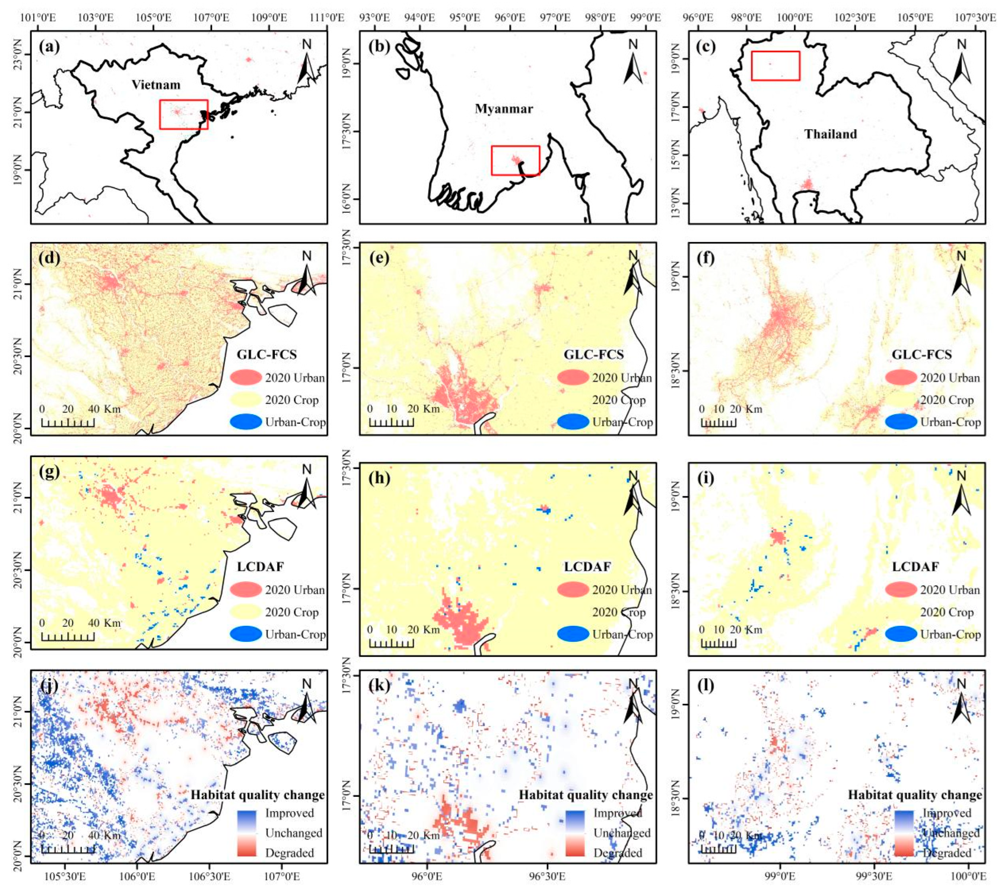
4.3. Urban Development and Habitat Quality

The rapid urbanization in the GMS over the past four decades has profoundly affected human societies and ecosystems. From 1980 to 2020, urban areas in the region expanded more than fourfold, primarily at the expense of arable land. Concurrently, during this urbanization phase, a significant transformation occurred where a considerable portion of urban lands was converted back into arable fields, accounting for nearly half of the GMS in 1980. According to the analysis of synergetic land-cover products, the reversion of urban areas to cropland predominantly occurred in rural locales distant from urban centers, most of which were scattered. To delve deeper into this phenomenon, we conducted detailed case studies in three emblematic regions: the Red River Delta in Vietnam, Yangon in Myanmar, and Chiang Mai in Thailand, as depicted in Figure 14. Due to the limited ability of our synergetic product to capture these small towns with a spatial resolution of 1 km, we combined GLC-FCS data for supplementary analysis. The data can be obtained as early as 1985, so the land cover change between 1985 and 2020 was displayed in Figure 14. These analyses aim to unpack the dynamics driving these land-use changes and explore their implications for urban development and habitat quality.

In the coastal vicinity of the Red River Delta, towns were generally dispersed with substantial areas where townland and cropland frequently interchanged, resulting in significant fragmentation of the land pattern. This region saw vigorous efforts toward land intensification, primarily to enhance rice cultivation and aquaculture efficiencies [64,65]. Such active development led to recurrent agricultural land-use modifications, reflecting a dynamic landscape where urbanization and agriculture continuously interact and reshape the region. On the outskirts of central Yangon and in more remote areas, we observed that many small towns were converted to cropland. GLC-FCS also captured a large amount of converted cropland within the central city of Yangon, near areas with abundant human activities, such as lakes and rivers. This trend is primarily attributed to conflicts between land management and production modes, driven by population migration and land policy changes. Initiated in 1990, Yangon’s poverty migration plan aimed to expand built-up areas. However, due to the high cost of living, most people opted not to relocate to the newly developed towns [66]. This led to a stalling in township development, with some plots earmarked for urban expansion transformed into paddy fields after 1995 [12]. The Asian financial crisis and subsequent shift of the capital city further exacerbated the challenges in land management, significantly impacting land transitions under urban development schemes [12]. In the comprehensive planning of urban development in Chiang Mai after the 1980s, the urban area growth was mainly based on the central expansion mode, while the area of high-density towns elsewhere decreased [67]. As a significant agricultural base during this period, Chiang Mai experienced a complex growth of cities that crossed planned land use boundaries.

Employing Pearson’s correlation analysis, we discerned a significantly negative correlation of −0.93 (p < 0.01) between urban area and the habitat quality index. Urban expansion notably brought about a decline in habitat quality, and this trend was somewhat mitigated by the rehabilitation of cropland that had been previously urbanized. This improvement was particularly evident in regions like the Red River Delta and Chiang Mai, where agricultural land was restored from urban and suburban areas. Although the rapid pace of urbanization inevitably exerts negative impacts on the ecological environment, strategic land management adjustments and ecological restoration initiatives can somewhat mitigate these adverse effects. Based on the spatial dynamics of urbanization-induced habitat quality change, future land use development plans should pay more attention to the balance between land management and ecological protection. Although land intensification development can to some extent prevent excessive expansion of urban land, it still needs to control the fragmentation of landscape patterns. In addition, the current level of afforestation is not sufficient to alleviate habitat degradation, governments of various countries in the GMS region need to actively formulate ecological protection priority development policies and expand nature reserves. These measures are crucial in balancing urban growth with environmental sustainability, ensuring that development does not come at the expense of ecological health.

5. Conclusions

The GMS has experienced rapid development, accompanied by significant changes in its natural environment over the past forty years. This study developed an ecological evaluation system that integrates the LCDAF and InVEST model for quantitative assessment of changes in land cover and habitat quality, along with an analysis of their underlying causes, to understand the overall ecological conditions in the GMS comprehensively. The following conclusions are drawn:

(i) The synergetic land cover dataset was produced by assimilating existing land cover products from 1980 to 2020, realizing a global accuracy of 73.9% and a regional accuracy of 80.4%. This dataset integrates the characteristics of different input data, providing a continuous time sequence of land cover and avoiding the noise caused by various adverse weather conditions and missing observation data. It can serve as a reliable foundation for habitat quality analysis in the GMS.

(ii) From our land cover results, cropland, grassland, shrubland, urban areas, and wetlands have experienced consistent growth, while forests, bareland, and water show a declining pattern. The decade from 1990 to 2000, aligned with the initiation of GMS economic cooperation, witnessed the most significant land cover conversions. The most substantial changes observed in the GMS were conversions between forest and cropland, characterized by intensive farming encroaching on ecological land and simultaneous afforestation resulting from the return of cropland.

(iii) In InVEST model analysis, overall habitat quality in the GMS declined over time, with Laos securing the highest ranking, followed by Myanmar, China, Cambodia, Vietnam, and Thailand. Rapid declines in habitat quality were attributed to extensive forest loss in Myanmar and Thailand. Conservation and reforestation policies in Cambodia and Guangxi, China, effectively mitigate habitat degradation.

(iv) From the perspective of landscape pattern, the habitat quality within the watershed was significantly and negatively influenced by land use intensity and landscape fragmentation, separately at a large and local spatial scale. While the GMS demonstrated dedication to ecological restoration, with certain regions displaying early signs of success, substantial challenges persist. The relevant government needs to further expand natural reserves and protect red lines while developing land intensification to prevent landscape fragmentation. The findings from our research provide valuable scientific evidence and reference data for regional ecological governance and planning.

References

1. Geist, H. Land-Use and Land-Cover Change: Local Processes to Global Impacts; Springer: Berlin/Heidelberg, Germany, 2006. [Google Scholar]
2. Kazak, J.K.J.S. The use of a decision support system for sustainable urbanization and thermal comfort in adaptation to climate change actions—The case of the Wrocław larger urban zone (Poland). Sustainability 2018, 10, 1083. [Google Scholar] [CrossRef]
3. Cegielska, K.; Noszczyk, T.; Kukulska, A.; Szylar, M.; Hernik, J.; Dixon-Gough, R.; Jombach, S.; Valánszki, I.; Kovács, K.F. Land use and land cover changes in post-socialist countries: Some observations from Hungary and Poland. Land Use Policy 2018, 78, 1–18. [Google Scholar] [CrossRef]
4. Duan, X.; Chen, Y.; Wang, L.; Zheng, G.; Liang, T. The impact of land use and land cover changes on the landscape pattern and ecosystem service value in Sanjiangyuan region of the Qinghai-Tibet Plateau. J. Environ. Manag. 2023, 325, 116539. [Google Scholar] [CrossRef]
5. Carvalho, S.; Oliveira, A.; Pedersen, J.S.; Manhice, H.; Lisboa, F.; Norguet, J.; de Wit, F.; Santos, F.D. A changing Amazon rainforest: Historical trends and future projections under post-Paris climate scenarios. Glob. Planet. Change 2020, 195, 103328. [Google Scholar] [CrossRef]
6. Nienhuis, J.H.; Ashton, A.D.; Edmonds, D.A.; Hoitink, A.; Kettner, A.J.; Rowland, J.C.; Törnqvist, T.E. Global-scale human impact on delta morphology has led to net land area gain. Nature 2020, 577, 514–518. [Google Scholar] [CrossRef]
7. Namkhan, M.; Gale, G.A.; Savini, T.; Tantipisanuh, N. Loss and vulnerability of lowland forests in mainland Southeast Asia. Conserv. Biol. 2021, 35, 206–215. [Google Scholar] [CrossRef]
8. Li, H.; Hong, L. Spatio-temporal land use/land cover dynamics and its driving forces in the Mekong Basin using Landsat imageries from 1988 to 2017. Geocarto Int. 2022, 37, 14676–14698. [Google Scholar] [CrossRef]
9. Sam, T.T.; Khoi, D.N. The responses of river discharge and sediment load to historical land-use/land-cover change in the Mekong River Basin. Environ. Monit. Assess. 2022, 194, 700. [Google Scholar] [CrossRef]
10. Spruce, J.; Bolten, J.; Mohammed, I.N.; Srinivasan, R.; Lakshmi, V. Mapping land use land cover change in the Lower Mekong Basin from 1997 to 2010. Front. Environ. Sci. 2020, 8, 21. [Google Scholar] [CrossRef]
11. Vu, H.T.D.; Tran, D.D.; Schenk, A.; Nguyen, C.P.; Vu, H.L.; Oberle, P.; Trinh, V.C.; Nestmann, F. Land use change in the Vietnamese Mekong Delta: New evidence from remote sensing. Sci. Total. Environ. 2022, 813, 151918. [Google Scholar] [CrossRef]
12. Cao, H.; Liu, J.; Chen, J.; Gao, J.; Wang, G.; Zhang, W. Spatiotemporal patterns of urban land use change in typical cities in the Greater Mekong Subregion (GMS). Remote Sens. 2019, 11, 801. [Google Scholar] [CrossRef]
13. Zhai, J.; Xiao, C.; Feng, Z.; Liu, Y. Spatio-Temporal Patterns of Land-Use Changes and Conflicts between Cropland and Forest in the Mekong River Basin during 1990–2020. Land 2022, 11, 927. [Google Scholar] [CrossRef]
14. He, B.; Wu, X.; Liu, K.; Yao, Y.; Chen, W.; Zhao, W. Trends in Forest Greening and Its Spatial Correlation with Bioclimatic and Environmental Factors in the Greater Mekong Subregion from 2001 to 2020. Remote Sens. 2022, 14, 5982. [Google Scholar] [CrossRef]
15. Ngo, K.D.; Lechner, A.M.; Vu, T.T. Land cover mapping of the Mekong Delta to support natural resource management with multi-temporal Sentinel-1A synthetic aperture radar imagery. Remote. Sens. Appl. Soc. Environ. 2020, 17, 100272. [Google Scholar] [CrossRef]
16. Townshend, J.R.; Masek, J.G.; Huang, C.; Vermote, E.F.; Gao, F.; Channan, S.; Sexton, J.O.; Feng, M.; Narasimhan, R.; Kim, D.; et al. Global characterization and monitoring of forest cover using Landsat data: Opportunities and challenges. Int. J. Digit. Earth 2012, 5, 373–397. [Google Scholar] [CrossRef]
17. Gong, P.; Wang, J.; Yu, L.; Zhao, Y.; Zhao, Y.; Liang, L.; Niu, Z.; Huang, X.; Fu, H.; Liu, S.; et al. Finer resolution observation and monitoring of global land cover: First mapping results with Landsat TM and ETM+ data. Int. J. Remote Sens. 2013, 34, 2607–2654. [Google Scholar] [CrossRef]
18. Pouliot, D.; Latifovic, R.; Zabcic, N.; Guindon, L.; Olthof, I. Development and assessment of a 250 m spatial resolution MODIS annual land cover time series (2000–2011) for the forest region of Canada derived from change-based updating. Remote Sens. Environ. 2014, 140, 731–743. [Google Scholar] [CrossRef]
19. Zhu, Z.; Woodcock, C.E. Continuous change detection and classification of land cover using all available Landsat data. Remote Sens. Environ. 2014, 144, 152–171. [Google Scholar] [CrossRef]
20. Fritz, S.; You, L.; Bun, A.; See, L.; McCallum, I.; Schill, C.; Perger, C.; Liu, J.; Hansen, M.; Obersteiner, M.J. Cropland for sub-Saharan Africa: A synergistic approach using five land cover data sets. Geophys. Res. Lett. 2011, 38. [Google Scholar] [CrossRef]
21. Tsendbazar, N.-E.; de Bruin, S.; Herold, M.J. Integrating global land cover datasets for deriving user-specific maps. Int. J. Digit. Earth 2017, 10, 219–237. [Google Scholar] [CrossRef]
22. Song, X.-P.; Huang, C.; Townshend, J.R. Improving global land cover characterization through data fusion. Geo-Spat. Inf. Sci. 2017, 20, 141–150. [Google Scholar] [CrossRef]
23. Jiang, J.; Ye, C.; Jin, Y.; Chen, Y. Estimation of carbon emissions in the Yangtze River Delta based on land cover data fusion. J. Appl. Remote. Sens. 2025, 19, 014508. [Google Scholar] [CrossRef]
24. Li, B.; Xu, X.; Liu, X.; Shi, Q.; Zhuang, H.; Cai, Y.; He, D.J. An improved global land cover mapping in 2015 with 30 m resolution (GLC-2015) based on a multi-source product fusion approach. Earth Syst. Sci. Data Discuss. 2022, 15, 2347–2373. [Google Scholar] [CrossRef]
25. Witjes, M.; Herold, M.; de Bruin, S. Iterative mapping of probabilities: A data fusion framework for generating accurate land cover maps that match area statistics. Int. J. Appl. Earth Obs. Geoinf. 2024, 131, 103932. [Google Scholar] [CrossRef]
26. Xu, G.; Chen, B. Generating a series of land covers by assimilating the existing land cover maps. J. Photogramm. Remote Sens. 2019, 147, 206–214. [Google Scholar] [CrossRef]
27. Costenbader, J.; Broadhead, J.; Yasmi, Y.; Durst, P.B. Drivers Affecting Forest Change in the Greater Mekong Subregion (GMS): An Overview; FAO: Rome, Italy, 2015. [Google Scholar]
28. Peng, J.; Xu, F.; Wu, J.; Deng, K.; Hu, T. Spatial differentiation of habitat quality in typical tourist city and their Influencing factors mechanisms: A case study of Huangshan City. Environ. Resour. 2019, 28, 2397–2409. [Google Scholar]
29. Hall, L.S.; Krausman, P.R.; Morrison, M.L. The habitat concept and a plea for standard terminology. Wildl. Soc. Bull. 1997, 25, 173–182. [Google Scholar]
30. Zheng, J.; Xie, B.; You, X. Spatio-temporal characteristics of habitat quality based on land-use changes in Guangdong Province. Acta Ecol. Sin. 2022, 42, 6997–7010. [Google Scholar]
31. Tripp, E.A.; Lendemer, J.C.; McCain, C.M. Habitat quality and disturbance drive lichen species richness in a temperate biodiversity hotspot. Oecologia 2019, 190, 445–457. [Google Scholar] [CrossRef] [PubMed]
32. Zhang, X.; Song, W.; Lang, Y.; Feng, X.; Yuan, Q.; Wang, J. Land use changes in the coastal zone of China’s Hebei Province and the corresponding impacts on habitat quality. Land Use Policy 2020, 99, 104957. [Google Scholar] [CrossRef]
33. De Simone, S.; Sigura, M.; Boscutti, F. Patterns of biodiversity and habitat sensitivity in agricultural landscapes. J. Environ. Plan. Manag. 2017, 60, 1173–1192. [Google Scholar] [CrossRef]
34. Tang, F.; Fu, M.; Wang, L.; Zhang, P. Land-use change in Changli County, China: Predicting its spatio-temporal evolution in habitat quality. Ecol. Indic. 2020, 117, 106719. [Google Scholar] [CrossRef]
35. Ding, Q.; Chen, Y.; Bu, L.; Ye, Y. Multi-scenario analysis of habitat quality in the Yellow River delta by coupling FLUS with InVEST model. Int. J. Environ. Res. Public Health 2021, 18, 2389. [Google Scholar] [CrossRef] [PubMed]
36. Wu, J.; Li, X.; Luo, Y.; Zhang, D. Spatiotemporal effects of urban sprawl on habitat quality in the Pearl River Delta from 1990 to 2018. Sci. Rep. 2021, 11, 13981. [Google Scholar] [CrossRef]
37. Yang, F.; Yang, L.; Fang, Q.; Yao, X. Impact of landscape pattern on habitat quality in the Yangtze River Economic Belt from 2000 to 2030. Ecol. Indic. 2024, 166, 112480. [Google Scholar] [CrossRef]
38. Berta Aneseyee, A.; Noszczyk, T.; Soromessa, T.; Elias, E. The InVEST habitat quality model associated with land use/cover changes: A qualitative case study of the Winike Watershed in the Omo-Gibe Basin, Southwest Ethiopia. Remote Sens. 2020, 12, 1103. [Google Scholar] [CrossRef]
39. Tang, F.; Wang, L.; Guo, Y.; Fu, M.; Huang, N.; Duan, W.; Luo, M.; Zhang, J.; Li, W.; Song, W. Spatio-temporal variation and coupling coordination relationship between urbanisation and habitat quality in the Grand Canal, China. Land Use Policy 2022, 117, 106119. [Google Scholar] [CrossRef]
40. Wu, J.; Luo, J.; Zhang, H.; Qin, S.; Yu, M. Projections of land use change and habitat quality assessment by coupling climate change and development patterns. Sci. Total Environ. 2022, 847, 157491. [Google Scholar] [CrossRef]
41. Davis, K.F.; Yu, K.; Rulli, M.C.; Pichdara, L.; D’Odorico, P. Accelerated deforestation driven by large-scale land acquisitions in Cambodia. Nat. Geosci. 2015, 8, 772–775. [Google Scholar] [CrossRef]
42. Johnston, R.; Lacombe, G.; Hoanh, C.T.; Noble, A.; Pavelic, P.; Smakhtin, V.; Suhardiman, D.; Kam, S.P.; Choo, P.S. Climate Change, Water and Agriculture in the Greater Mekong Subregion; International Water Management Institute: Colombo, Sri Lanka, 2010. [Google Scholar]
43. Ming, W.; Luo, X.; Luo, X.; Long, Y.; Xiao, X.; Ji, X.; Li, Y. Quantitative Assessment of Cropland Exposure to Agricultural Drought in the Greater Mekong Subregion. Remote Sens. 2023, 15, 2737. [Google Scholar] [CrossRef]
44. Congalton, R.G.; Green, K. Assessing the Accuracy of Remotely Sensed Data: Principles and Practices; CRC Press: Boca Raton, FL, USA, 2019. [Google Scholar]
45. Moreira, M.; Fonseca, C.; Vergílio, M.; Calado, H.; Gil, A.J. Spatial assessment of habitat conservation status in a Macaronesian island based on the InVEST model: A case study of Pico Island (Azores, Portugal). Land Use Policy 2018, 78, 637–649. [Google Scholar] [CrossRef]
46. Wu, J.; Wang, X.; Zhong, B.; Yang, A.; Jue, K.; Wu, J.; Zhang, L.; Xu, W.; Wu, S.; Zhang, N. Ecological environment assessment for Greater Mekong Subregion based on Pressure-State-Response framework by remote sensing. Ecol. Indic. 2020, 117, 106521. [Google Scholar] [CrossRef]
47. Wei, Q.; Abudureheman, M.; Halike, A.; Yao, K.; Yao, L.; Tang, H.; Tuheti, B. Temporal and spatial variation analysis of habitat quality on the PLUS-InVEST model for Ebinur Lake Basin, China. Ecol. Indic. 2022, 145, 109632. [Google Scholar] [CrossRef]
48. Bai, L.; Xiu, C.; Feng, X.; Liu, D. Influence of urbanization on regional habitat quality: A case study of Changchun City. Habitat Int. 2019, 93, 102042. [Google Scholar] [CrossRef]
49. Lindenmayer, D.; Hobbs, R.J.; Montague-Drake, R.; Alexandra, J.; Bennett, A.; Burgman, M.; Cale, P.; Calhoun, A.; Cramer, V.; Cullen, P.; et al. A checklist for ecological management of landscapes for conservation. Ecol. Lett. 2008, 11, 78–91. [Google Scholar] [CrossRef] [PubMed]
50. Forman, R.T. Estimate of the area affected ecologically by the road system in the United States. Conserv. Biol. 2000, 14, 31–35. [Google Scholar] [CrossRef]
51. McGarigal, K. FRAGSTATS: Spatial Pattern Analysis Program for Quantifying Landscape Structure; US Department of Agriculture, Forest Service, Pacific Northwest Research Station: Corvallis, OR, USA, 1995; Volume 351. [Google Scholar]
52. Chen, B.; Kayiranga, A.; Ge, M.; Ciais, P.; Zhang, H.; Black, A.; Xiao, X.; Yuan, W.; Zeng, Z.; Piao, S. Anthropogenic activities dominated tropical forest carbon balance in two contrary ways over the Greater Mekong Subregion in the 21st century. Glob. Change Biol. 2023, 29, 3421–3432. [Google Scholar] [CrossRef]
53. Brandt, M.; Yue, Y.; Wigneron, J.P.; Tong, X.; Tian, F.; Jepsen, M.R.; Xiao, X.; Verger, A.; Mialon, A.; Al-Yaari, A. Satellite-observed major greening and biomass increase in south China karst during recent decade. Earth’s Future 2018, 6, 1017–1028. [Google Scholar] [CrossRef]
54. Delang, C.O.; Yuan, Z. China’s Grain for Green Program; Springer: Berlin/Heidelberg, Germany, 2016. [Google Scholar]
55. Tong, X.; Brandt, M.; Yue, Y.; Ciais, P.; Rudbeck Jepsen, M.; Penuelas, J.; Wigneron, J.-P.; Xiao, X.; Song, X.-P.; Horion, S. Forest management in southern China generates short term extensive carbon sequestration. Nat. Commun. 2020, 11, 129. [Google Scholar] [CrossRef]
56. Tong, X.; Brandt, M.; Yue, Y.; Horion, S.; Wang, K.; Keersmaecker, W.D.; Tian, F.; Schurgers, G.; Xiao, X.; Luo, Y. Increased vegetation growth and carbon stock in China karst via ecological engineering. Nat. Sustain. 2018, 1, 44–50. [Google Scholar] [CrossRef]
57. Feng, Y.; Ziegler, A.D.; Elsen, P.R.; Liu, Y.; He, X.; Spracklen, D.V.; Holden, J.; Jiang, X.; Zheng, C.; Zeng, Z. Upward expansion and acceleration of forest clearance in the mountains of Southeast Asia. Nat. Sustain. 2021, 4, 892–899. [Google Scholar] [CrossRef]
58. Grogan, K.; Pflugmacher, D.; Hostert, P.; Mertz, O.; Fensholt, R. Unravelling the link between global rubber price and tropical deforestation in Cambodia. Nat. Plants 2019, 5, 47–53. [Google Scholar] [CrossRef]
59. Lu, F.; Hu, H.; Sun, W.; Zhu, J.; Liu, G.; Zhou, W.; Zhang, Q.; Shi, P.; Liu, X.; Wu, X. Effects of national ecological restoration projects on carbon sequestration in China from 2001 to 2010. Proc. Natl. Acad. Sci. USA 2018, 115, 4039–4044. [Google Scholar] [CrossRef]
60. Xu, H.; Liu, K.; Ning, T.; Huang, G.; Zhang, Q.; Li, Y.; Wang, M.; Fan, Y.; An, W.; Ji, L.; et al. Environmental remediation promotes the restoration of biodiversity in the Shenzhen Bay Estuary, South China. Ecosyst. Health 2022, 8, 2026250. [Google Scholar] [CrossRef]
61. Sallustio, L.; De Toni, A.; Strollo, A.; Di Febbraro, M.; Gissi, E.; Casella, L.; Geneletti, D.; Munafò, M.; Vizzarri, M.; Marchetti, M. Assessing habitat quality in relation to the spatial distribution of protected areas in Italy. J. Environ. Manag. 2017, 201, 129–137. [Google Scholar] [CrossRef] [PubMed]
62. Kowarik, I. Novel urban ecosystems, biodiversity, and conservation. Environ. Pollut. 2011, 159, 1974–1983. [Google Scholar] [CrossRef]
63. Pesola, L.; Cheng, X.; Sanesi, G.; Colangelo, G.; Elia, M.; Lafortezza, R. Linking above-ground biomass and biodiversity to stand development in urban forest areas: A case study in Northern Italy. Landsc. Urban Plan. 2017, 157, 90–97. [Google Scholar] [CrossRef]
64. Morton, L.W. Working toward sustainable agricultural intensification in the Red River Delta of Vietnam. J. Soil Water Conserv. 2020, 75, 109A–116A. [Google Scholar] [CrossRef]
65. Pretty, J. Intensification for redesigned and sustainable agricultural systems. Science 2018, 362, eaav0294. [Google Scholar] [CrossRef]
66. Nwe, T.T. Yangon: The emergence of a new spatial order in Myanmar’s capital city. Sojourn J. Soc. Issues Southeast Asia 1998, 86–113. [Google Scholar] [CrossRef]
67. McGrath, B.; Sangawongse, S.; Thaikatoo, D.; Barcelloni Corte, M. The architecture of the metacity: Land use change, patch dynamics and urban form in Chiang Mai, Thailand. Urban Plan. 2017, 2, 53–71. [Google Scholar] [CrossRef]
68. Loveland, T.; Brown, J.; Ohlen, D.; Reed, B.; Zhu, Z.; Yang, L.; Howard, S.; Hall, F.; Collatz, G.; Meeson, B.W.; et al. ISLSCP II IGBP DISCover and SiB Land Cover, 1992–1993; ORNL DAAC: Oak Ridge, TN, USA, 2009. [Google Scholar]
69. Bartholome, E.; Belward, A.S. GLC2000: A new approach to global land cover mapping from Earth observation data. Int. J. Remote Sens. 2005, 26, 1959–1977. [Google Scholar] [CrossRef]
70. Hansen, M.C.; DeFries, R.S.; Townshend, J.R.; Sohlberg, R. Global land cover classification at 1 km spatial resolution using a classification tree approach. Int. J. Remote Sens. 2000, 21, 1331–1364. [Google Scholar] [CrossRef]
71. Bontemps, S.; Boettcher, M.; Brockmann, C.; Kirches, G.; Lamarche, C.; Radoux, J.; Santoro, M.; Vanbogaert, E.; Wegmüller, U.; Herold, M.; et al. Multi-year global land cover mapping at 300 m and characterization for climate modelling: Achievements of the Land Cover component of the ESA Climate Change Initiative. Int. Arch. Photogramm. Remote Sens. Spat. Inf. Sci. 2015, 40, 323–328. [Google Scholar] [CrossRef]
72. Friedl, M.A.; Sulla-Menashe, D.; Tan, B.; Schneider, A.; Ramankutty, N.; Sibley, A.; Huang, X. MODIS Collection 5 global land cover: Algorithm refinements and characterization of new datasets. Remote Sens. Environ. 2010, 114, 168–182. [Google Scholar] [CrossRef]
Figure 1. Geographic location of the Greater Mekong Subregion highlighting elevation characteristics from SRTM data.
Remotesensing 17 01467 g001
Figure 2. Confusion matrix of classification results of the Greater Mekong Subregion in 2020.
Remotesensing 17 01467 g002
Figure 3. Annual area of all land cover types in the Greater Mekong Subregion from 1980–2020.
Remotesensing 17 01467 g003
Figure 4. Area change rates of major land cover types in different countries or regions of the Greater Mekong Subregion from 1980 to 2020.
Remotesensing 17 01467 g004
Figure 5. Spatial distribution of land cover types and their conversions in the Greater Mekong Subregion from 1980–2020. (ae) respectively represent land cover types at different times. (f) represents significant land cover conversions between 1980 and 2020. Fo, Sh, Gr, and Cr are the abbreviations of forest, shrubland, grassland, and cropland.
Remotesensing 17 01467 g005
Figure 6. Significant conversions on major land cover types in the Greater Mekong Subregion occurred between 1980 and 2020. The streams denote the process of conversions, with width reflecting the magnitude of conversions. The numerical values represent the total conversions area involving specific land cover types for a given year.
Remotesensing 17 01467 g006
Figure 7. Area proportion of major land cover types in different countries or regions of the Greater Mekong Subregion from 1980 to 2020.
Remotesensing 17 01467 g007
Figure 8. Spatial distribution of habitat quality and its change in the Greater Mekong Subregion from 1980 to 2020.
Remotesensing 17 01467 g008
Figure 9. Spatial distribution of habitat quality level and its change in the Greater Mekong Subregion from 1980 to 2020.
Remotesensing 17 01467 g009
Figure 10. Area with habitat quality level in the Greater Mekong Subregion from 1980 to 2020.
Remotesensing 17 01467 g010
Figure 11. Variations of habitat quality and landscape pattern indexes across different countries or regions in the Greater Mekong Subregion from 1980 to 2020.
Remotesensing 17 01467 g011
Figure 12. Spatial distribution of habitat degradation degree and its change from 1980 to 2020 in the Greater Mekong Subregion.
Remotesensing 17 01467 g012
Figure 13. The uncertainty of different parameters in a habitat quality module of InVEST model.
Remotesensing 17 01467 g013
Figure 14. Spatial distribution of land cover and habitat quality change from 1980 to 2020 in typical regions in the Greater Mekong Subregion. The three columns of figures from left to right represent the Red River Delta in Vietnam, Yangon in Myanmar, and Chiang Mai in Thailand, respectively. (ac) represent the relative position of the typical regions in their countries. (df) show the land cover and its conversion of GLC-FCS from 1985 to 2020. (gi) show the land cover and the conversion of our LCDAF from 1980 to 2020. (jl) show the change in habitat quality based on LCDAF from 1980 to 2020.
Remotesensing 17 01467 g014