Article

Cover Crop Types Influence Biomass Estimation Using Unmanned Aerial Vehicle-Mounted Multispectral Sensors

by
Sk Musfiq Us Salehin
,
Chiranjibi Poudyal
,
Nithya Rajan
* and
Muthukumar Bagavathiannan
Department of Soil and Crop Sciences, Texas A&M University, College Station, TX 77843, USA
*
Author to whom correspondence should be addressed.
Remote Sens. 2025, 17(8), 1471; https://doi.org/10.3390/rs17081471
Submission received: 25 February 2025 / Revised: 12 April 2025 / Accepted: 18 April 2025 / Published: 20 April 2025
(This article belongs to the Special Issue Perspectives of Remote Sensing for Precision Agriculture)

Abstract

:
Accurate cover crop biomass estimation is critical for evaluating their ecological benefits. Traditional methods, like destructive sampling, are labor-intensive and time-consuming. This study investigates the application of unmanned aerial vehicle (UAV)-mounted multispectral sensors to estimate biomass in oats, Austrian winter peas (AWP), turnips, and a combination of all three crops across six experimental plots. Five spectral images were collected at two growth stages, analyzing band reflectance, nine vegetation indices, and canopy height models (CHMs) for biomass estimation. Results indicated that most vegetation indices were effective during mid-growth stages but showed reduced accuracy later. Stepwise multiple linear regression revealed that combining the normalized difference red-edge (NDRE) index and CHM provided the best biomass model before termination (R2 = 0.84). For bitemporal images, green reflectance, CHM, and the ratio of near-infrared (NIR) to red achieved the best performance (R2 = 0.85). Cover crop species also influenced the model performance. Oats were best modeled using the enhanced vegetation index (EVI) (R2 = 0.86), AWP with red-edge reflectance (R2 = 0.71), turnips with NIR, GNDVI, and CHM (R2 = 0.95), and mixed species with NIR and blue band reflectance (R2 = 0.93). These findings demonstrate the potential of high-resolution multispectral imaging for efficient biomass assessment in precision agriculture.

1. Introduction

Cover crops in cropping systems are grown between cash crop seasons to incorporate into the soil or left as mulches before maturity. They provide several ecosystem services, including reduced soil erosion, improved soil health, carbon sequestration, weed suppression, and increased crop yield [1,2,3]. However, most of these benefits from cover crops depend on the amount of biomass they produce at termination [2,4,5,6].
The quantity of cover crop biomass produced determines the extent of the ecosystem services. For example, increased biomass of cover crops provides more soil cover, thus reducing soil erosion [7,8]. Weed suppression from cover crops increases with increasing biomass production [5,6]. Similarly, increased biomass of cover crops upon incorporation into the soil increases soil carbon sequestration [9,10]. Therefore, quantifying the aboveground biomass is essential, as it also estimates the belowground biomass and overall biomass production of cover crops [11,12].
The conventional approach to quantifying cover crop biomass involves hand sampling from a few spots and measuring the dry mass to estimate the biomass of the entire field. This destructive method is laborious, time-consuming, and subject to error. Therefore, the use of advanced non-destructive techniques is necessary for quantifying and mapping the aboveground biomass of large agricultural fields [13,14]. Moreover, using the shoot-to-root ratio of specific crops, we can estimate and model the overall biomass of different cover crops.
Several remote sensing techniques can be used to model the cover crop biomass. For example, multispectral images from Landsat-8 showed that vegetation indices based on red, green, blue, and near-infrared (NIR) reflectance can be used to estimate oat–radish biomass [15]. On the other hand, short-wave infrared-based vegetation indices from Sentinel-2 have been shown to have better estimation accuracy for various cover crop biomass types [16,17]. However, the low spatial resolution of satellite images makes it harder to estimate biomass precisely, especially for smaller-scale agricultural fields. On the other hand, high-resolution multispectral images from unmanned aerial vehicles (UAVs) can help address this issue in precision agricultural management.
One of the major advantages of using UAVs for crop phenotyping is the ability to utilize crop canopy height models (CHMs) and achieve high spatial resolutions [18]. Several studies have found promising results from CHMs on UAVs in estimating different cover crop biomass. However, their efficiency varies widely depending on the crop types and growth stages [19,20,21,22]. These conflicting findings suggest a need for improved crop species performance of CHMs and their utility in modeling biomass using vegetation indices.
The common vegetation indices used for biomass estimation have been unsuccessful due to index saturation at the later growth stages of the crops [14,23,24]. As the canopies cover the field, it becomes difficult to quantify the biomass using NIR band reflectance [18,25]. Moreover, the performance of these vegetation indices depends on the type of crop [22,26,27,28]. Therefore, crop-specific investigations are needed to understand the performance of different vegetation indices and CHMs in estimating biomass. Moreover, it is unknown how combining spectral signatures with CHMs can be used to model the biomass of different cover crops.
In this study, we used multispectral sensors mounted on a UAV to estimate the biomass of brassica, legume, grass, and three-species mix cover crops. These species have vastly different canopy structures. Therefore, identifying species-specific models is crucial for estimating their biomass and overall ecosystem services. Often, these species are mixed as a cover crop for multiple benefits, such as nitrogen fixation from legumes and deeper root systems from grasses [29,30]. Therefore, mixed-species cover crops are considered a climate-smart practice in cropping systems. However, estimating their biomass using remote-sensing techniques can be challenging due to complex canopy structure and spectral signatures from multiple species [16,23]. Using high-resolution multispectral images from UAVs can potentially capture such complex canopy structures and model biomass effectively. A few studies have investigated the efficiency of UAV-derived images in modeling grass, brassica, and legume species mixtures [27,31,32]. However, there is no study investigating the efficiency of UAVs to estimate the biomass of Austrian winter peas, turnips, and a tri-species mix of oats, Austrian winter peas, and turnips.
Our goal for this study was to use different band reflectance, vegetation indices, and CHMs to model the biomass of cover crops. Our specific objectives were (1) to identify the best model to estimate cover crop biomass at different growth stages from bitemporal multispectral images and (2) to study the influence of cover crop types on the model performance of biomass estimation through multispectral images.

2. Materials and Methods
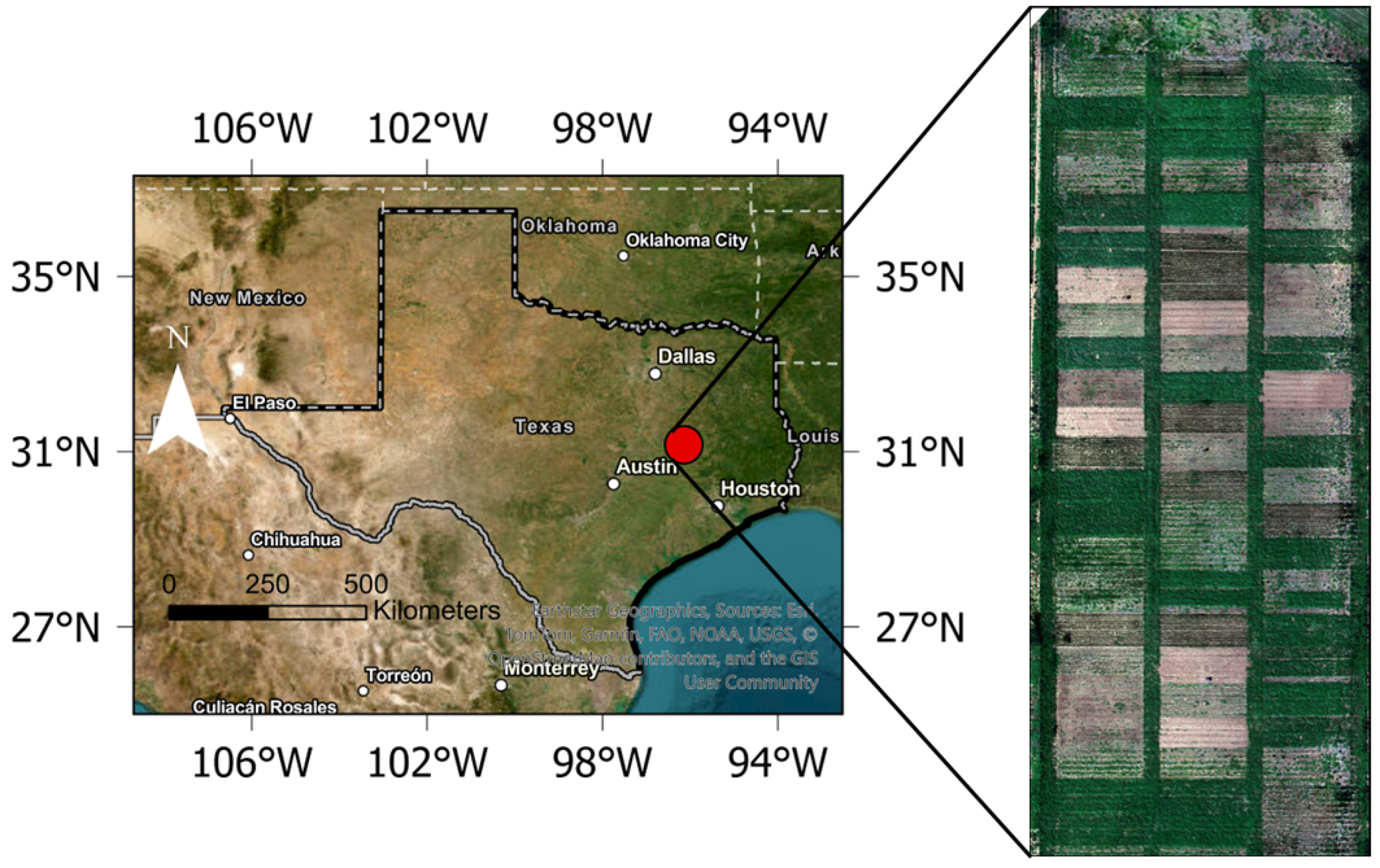
2.1. Study Site

The study was conducted at the Texas A&M University Research Farm near College Station, Texas (30°33′6.69′′N, 96°25′57′′W, 68 m above mean sea level). The study site is located on the Brazos River floodplains and within the East Central Texas Plains ecoregion (Figure 1). The site’s climate is characterized as humid subtropical, with an average annual precipitation of 1060 mm and an average annual temperature of 20.6 °C [33]. The soil at the site is classified as Belk Clay (fine, mixed, active, thermic Entic Hapluderts) with a 0–1% slope and a silty clay or clay texture in the A and B master horizons [34].
The cover crops were established as part of an organic cotton field experiment initiated in 2020. The field study employed a randomized split-plot design, with tillage practices as main plots (conventional and minimum tillage) and cover crop management as subplots, replicated three times. However, the effect of the tillage practices was not considered in this study. Therefore, each cover crop type was replicated six times in the experimental design. Each experimental plot was 50 m × 8 m in size. Details of the field experiment can be found in Salehin, Rajan [30].
Cover crops planted in the cotton field were Austrian winter pea (Pisum sativum), which is a legume; purple-top turnip (Brassica rapa subsp. rapa); and oats (Avena sativa L.), both of which are non-legumes. A mix of all three cover crops was also compared with the monoculture cover crops. Two seasons of cover crops were studied to train and validate the models for biomass estimation. Cover crops grown in the 2021–2022 season were used to train the model, whereas cover crops from the 2020–2021 season were used to validate the model. During the 2020–2021 season, cover crops were planted on 4 November 2020 and terminated on 6 April 2021. Similarly, during the 2021–2022 season, the cover crops were planted on 19 November 2021 and terminated on 6 April 2022. Cover crop biomass samples were collected on 1 March and 1 April 2022 to train the models and to validate the models on 31 March 2021.
For both years, cover crop biomass samples were collected using two 0.5 × 0.5 m quadrants from each plot, a day after the flights. The two samples from each plot were taken randomly and merged to take the average for each plot. The biomass samples were oven-dried at 60 °C for at least three days or until a constant mass was observed. The dry mass of samples from each plot was recorded for use in modeling with UAV images.

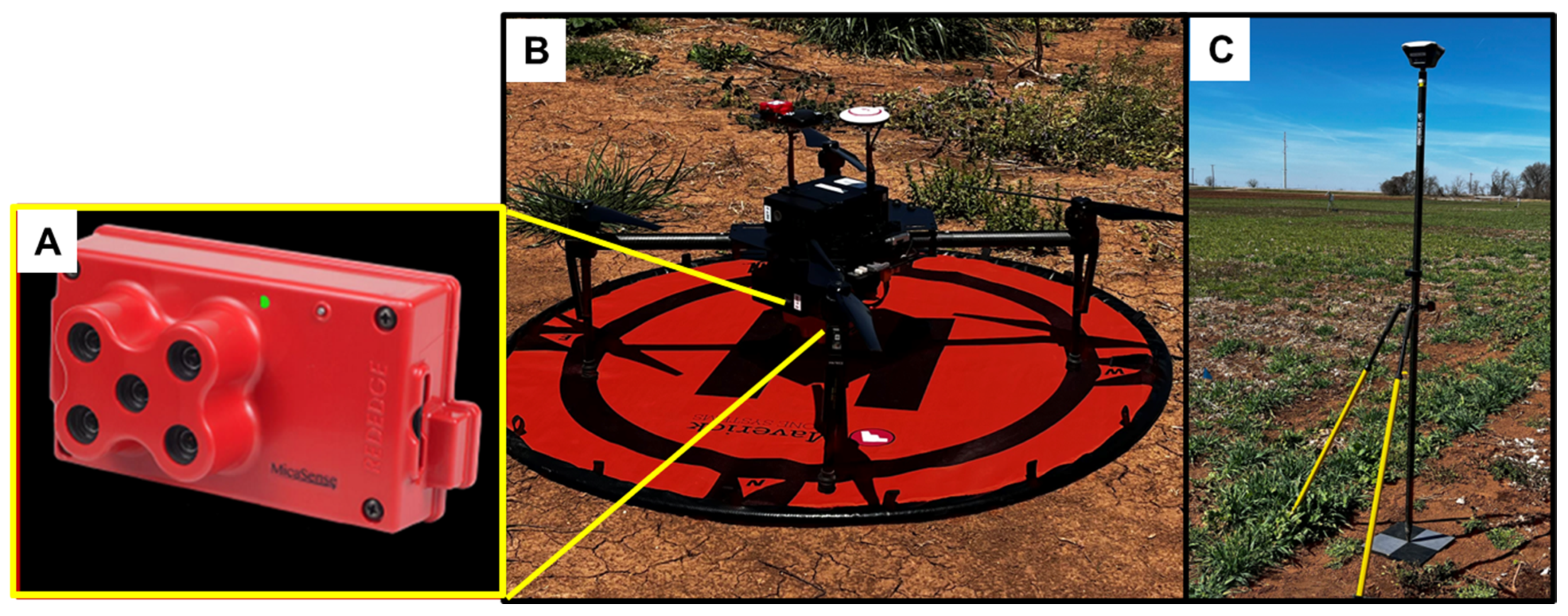
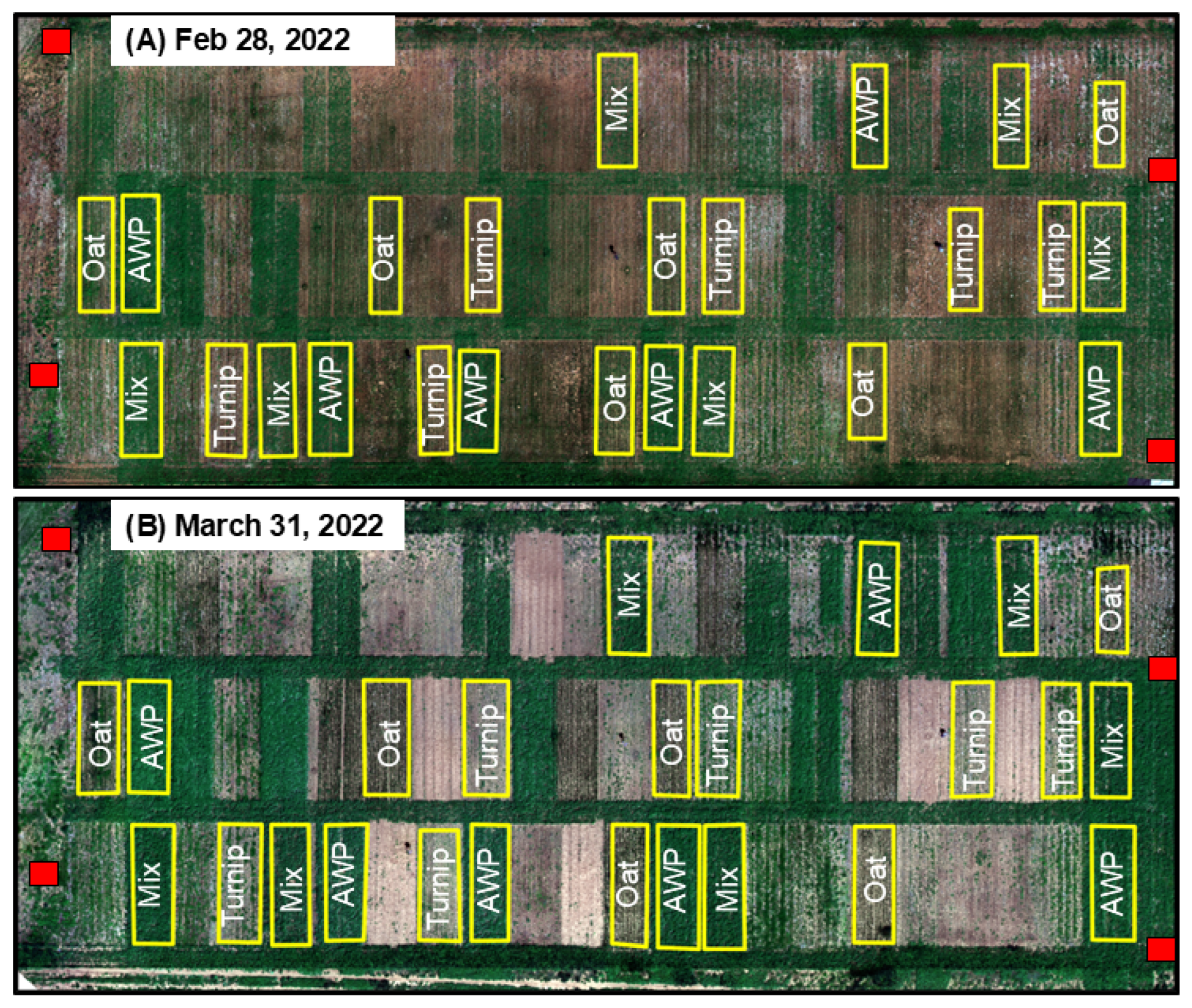
2.2. Image Acquisition

The images were collected using a five-spectral-band camera from MicaSense (RedEdge-3, MicaSense Inc., Seattle, WA, USA). The five spectral bands, along with their central wavelengths and bandwidths, are presented in Table 1. The camera system utilized a 5.4 mm focal length and a 4.8 mm × 3.36 mm complementary metal oxide semiconductor (CMOS) sensor (Figure 2A). The camera was mounted on a UAV or quadcopter (Matrice 100, SZ DJI Technology Ltd., Shenzhen, China) (Figure 2B). The images were collected on 28 February and 31 March 2022 at the mid and late-growth stages of the cover crops to train the models. UAV images were collected on 30 March 2021 to validate the models.
The flights were conducted at a height of 30 m above ground with 75% front and side overlaps. The spatial resolution, or ground sampling distance, of the images was 2 cm, meaning that each pixel covered a 2 × 2 cm2 area on the ground. The UgCS flight planning app (SPH Engineering, Riga, Latvia) was used to plan flight missions using an automated route. Four ground control points (GCPs) were laid on four corners of the field in a zigzag pattern before the flights for accurate georeferencing for image processing (Figure 3). GPS coordinates and elevations of the GCPs were collected using a real-time kinematics (RTK) system (Reach RS+, Emlid Ltd., Saint Petersburg, Russia) configured with a Trimble network (Figure 2C).

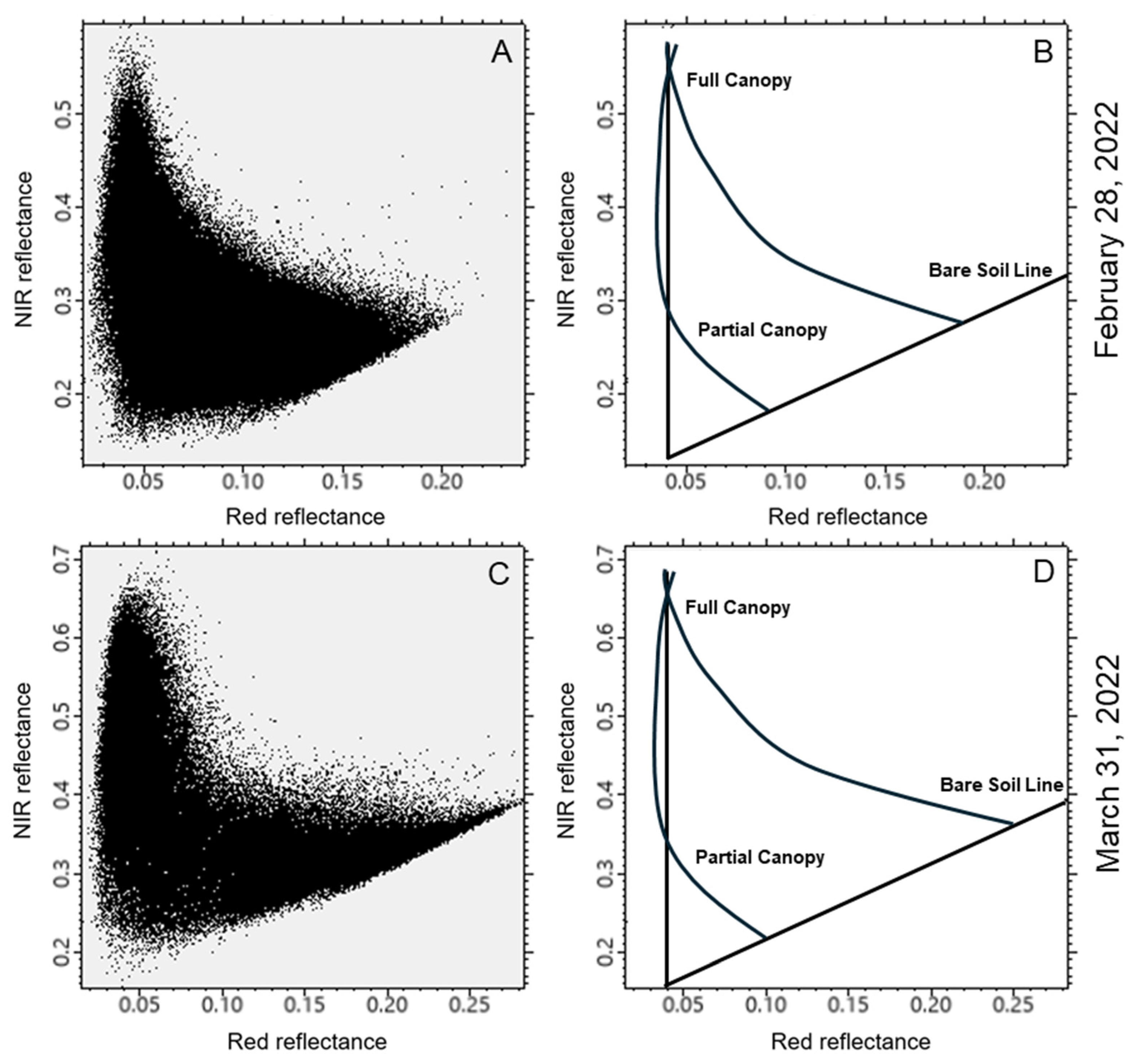
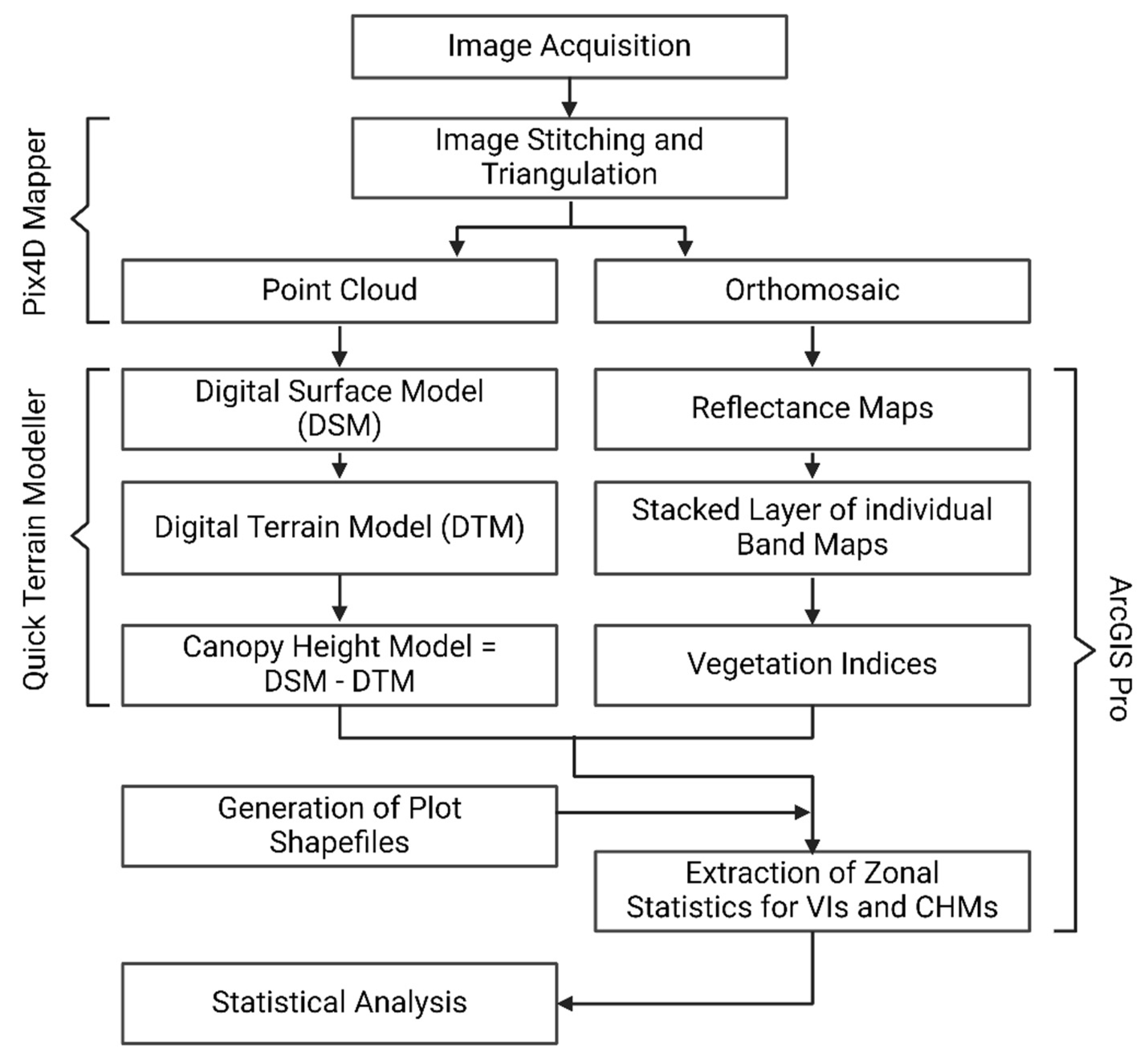
2.3. Image Processing Approach

A total of 315 images were collected for each band on 28 February, and 312 images were collected on 31 March. On the other hand, for 30 March 2021, a total of 317 images were collected. Imagery for each date was processed using Pix4Dmapper (version 4.9.0, Prilly, Switzerland) in three major steps. In the first step, identifiable features were extracted as key points. Following this, the images were calibrated based on the camera model and geolocation of GCPs. In the second step, densified point clouds were produced using the tie points from the first step. The orthomosaic image was the product of the orthorectification process, which corrects lens distortion, camera tilt, perspective, and relief displacement [35]. The band reflectance values were adjusted based on calibration panel images captured at the start and end of each flight. The known reflectance values of the panel for each band are used to calibrate the camera reflectance. The final result was an orthomosaic dataset of single-band reflectance of blue, green, red, red edge, and NIR.
Individual plot shapefiles were created for each image acquisition date using ArcGIS Pro [36]. The overall statistics of individual band reflectance, including mean, were extracted using the plot shapefiles and the zonal statistics function in ArcGIS. The five single-band images were layered into a composite band for each date. The composite band was used to generate different vegetation indices using the band arithmetic tool in ArcGIS (Figure 4). The details of the calculated vegetation indices are provided in Table 2.
A rough triangular distribution of points was observed in the scatterplot when NIR reflectance was plotted against the corresponding red band reflectance (Figure 5A,C). This pattern is associated with the reflectance characteristics of vegetation and soil and the mixing of these characteristics within the image pixels. The diagrammatic triangular representation shows the features of the images in the distribution (Figure 5B,D). The bare soil areas within the images lie along the diagonal base of the triangle (Figure 5B,D). In contrast, pixels representing living vegetation are positioned in the upper-left region of the distribution. This distribution arises because living vegetation strongly absorbs light in the red spectral band while reflecting strongly in the NIR band [44]. However, the pixel distribution for soil and the full canopy does not always form straight lines, as shown in Figure 5B,D. The intercept (a) and slope (b) of this bare soil line for each imagery are considered to calculate the perpendicular vegetation index (PVI).
The canopy height models (CHMs) were generated using Structure from Motion (SfM) point clouds created in Pix4Dmapper. Pix4D uses overlapped images to detect key points across multiple images. It then uses the known coordinates of the GCPs to match these key points to determine their relative position based on X, Y, and Z axes, which represent latitude, longitude, and elevation, respectively. Pix4D also outputs a digital surface model based on the densified point clouds. For further processing, the point cloud data were imported into Quick Terrain Modeler [45]. There, the original Z values (elevation) were then converted into the above-ground level (AGL) by subtracting the digital surface model from the original Z values using the AGL analyst tool. This AGL dataset was then used to create a gridded surface model representing the CHM. The February and March CHMs were generated at sampling distances of 11 and 10 cm, respectively (Figure 4B,D). Similarly, the CHMs for March 2021 images were generated at a sampling distance of 10 cm. Canopy height statistics were extracted from the CHMs using the shapefiles and the “Zonal Statistics as Table” function of ArcGIS. We considered the mean values of zonal statistics because of their high correlation with biomass. The detailed steps of image processing are shown in Figure 6.

2.4. Statistical Analyses
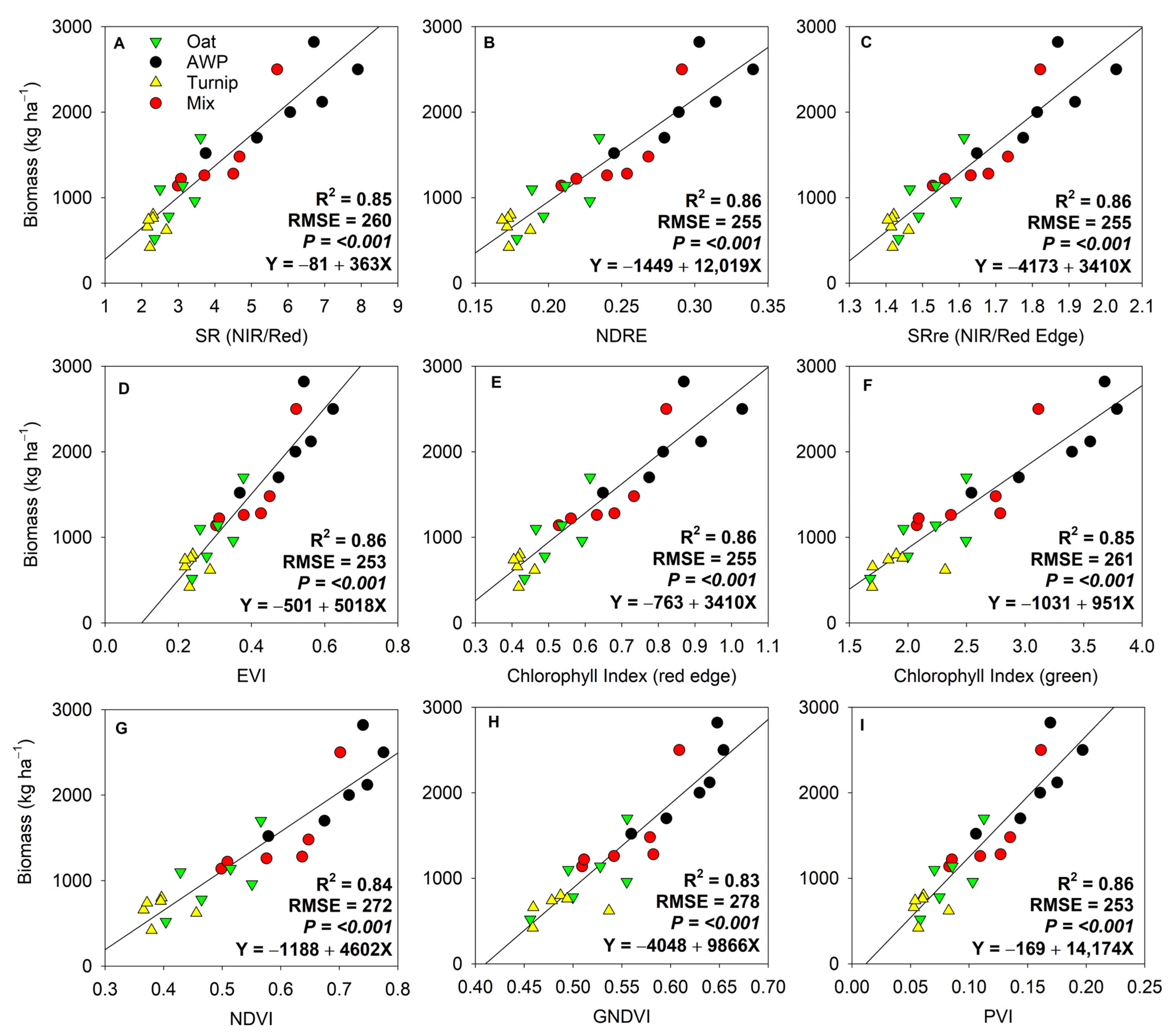
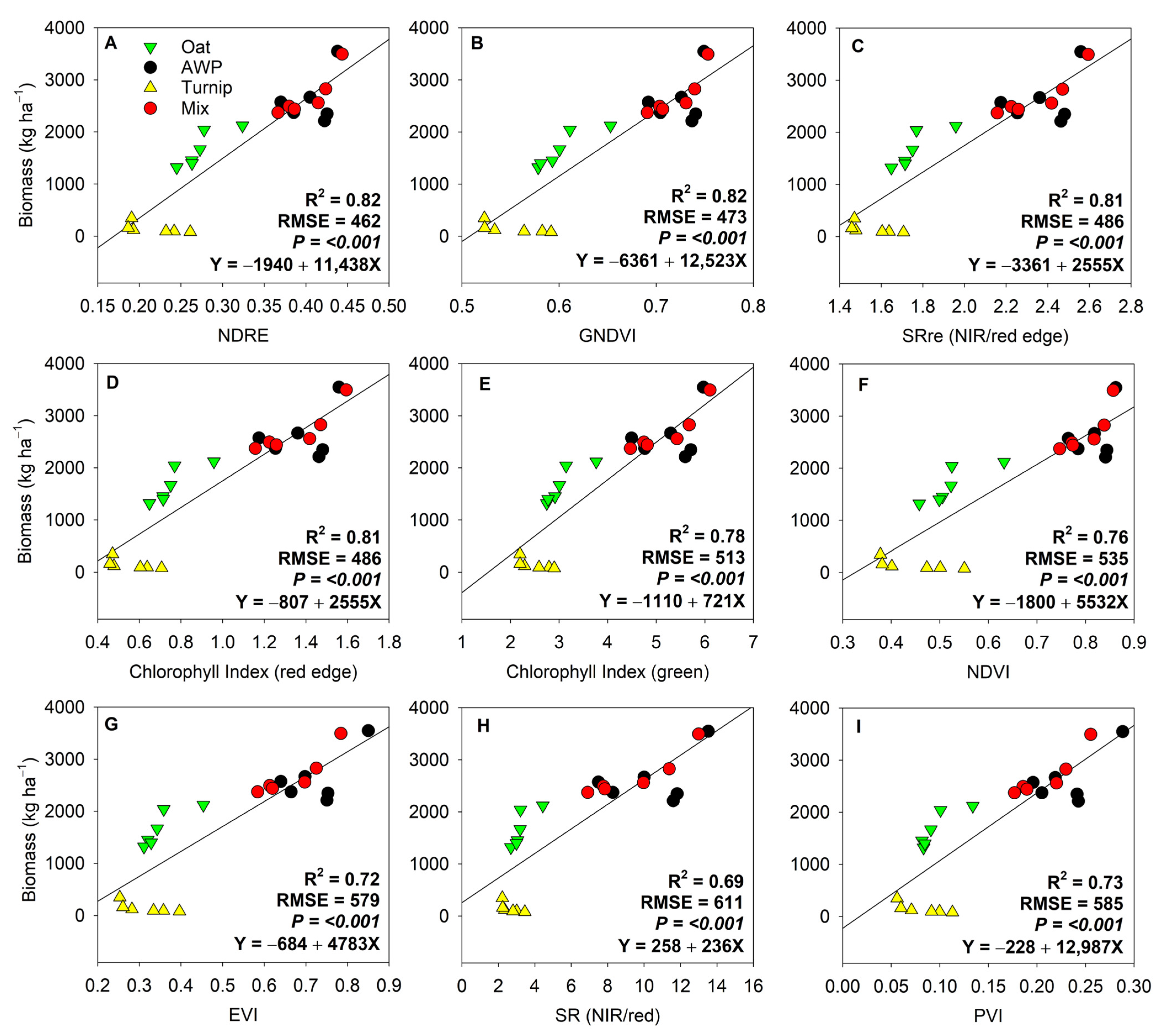
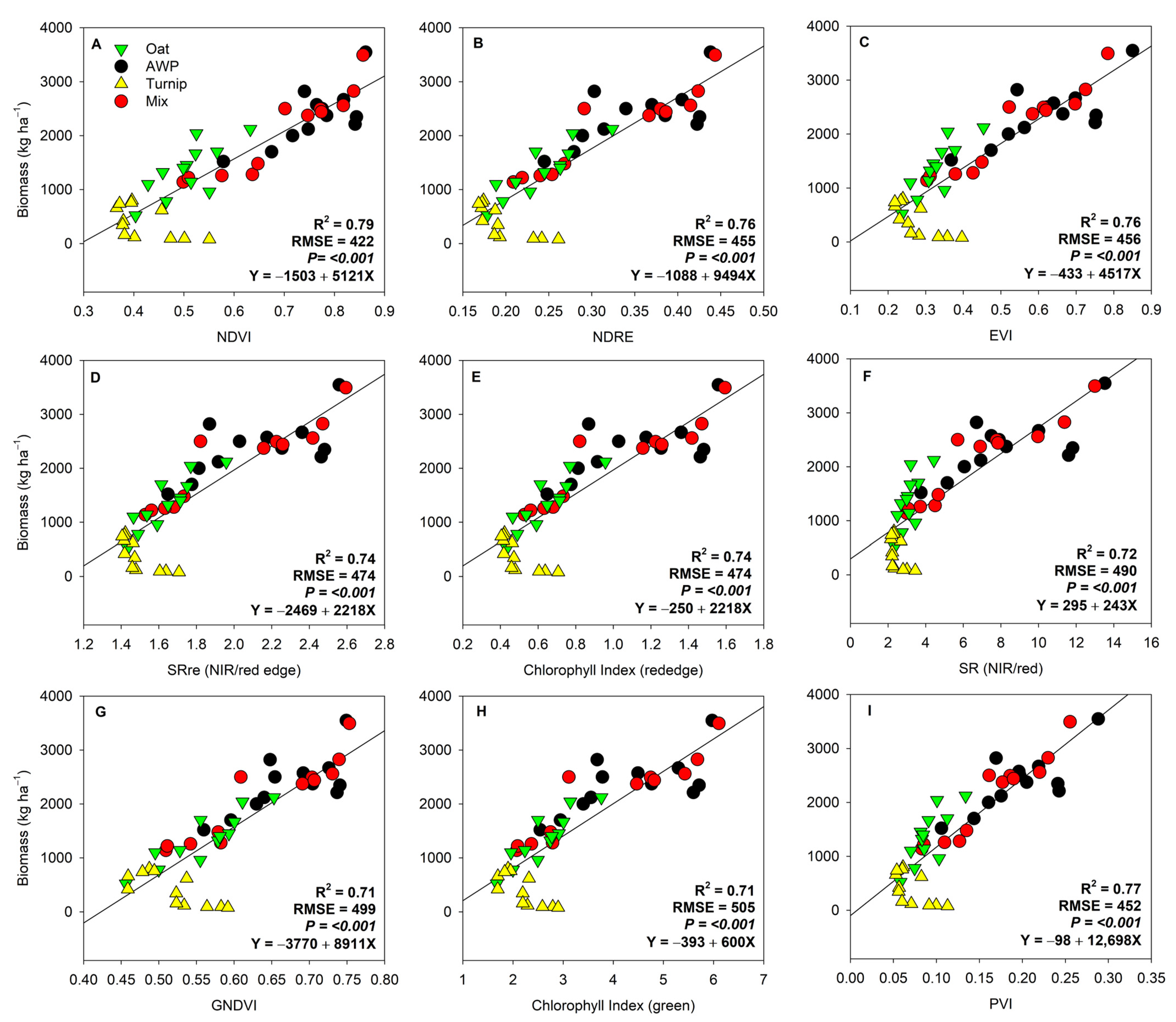
The mean values of the individual band reflectance, vegetation indices, and CHMs extracted from the plot shapefiles were used to model the biomass of cover crops. All statistical analyses were performed in R version 4.4.1 [46]. First, the correlation among the variables, including the cover crop biomass, band reflectance, vegetation indices, and CHMs, was investigated using the CORRPLOT package in R [47]. Later, simple linear regression models were fitted for each vegetation index and CHM to estimate biomass.
To determine the best-fit model, bidirectional stepwise multiple linear regression was performed separately for each date and cover crop type, based on p-values. For that, the biomass was modeled with all reflectance bands, nine vegetation indices, and the CHM. Then, both forward and backward stepwise regression were performed, using a p-value of 0.15 to enter and remove variables from the model. The stepwise regression was performed using the OLSRR package (version 0.6.0) in R [48]. The adjusted R2 and root mean square error (RMSE) of these models were assessed to determine their performance. Due to the high correlation among some of the vegetation indices, we examined the variance inflation factor (VIF) for each model using the CAR package (version 3.1-3) in R [49]. If the VIF was greater than 15 for a variable, one or more variables were removed from the model based on their correlation with biomass, thereby reducing the VIF of all variables without significantly compromising the model fit.

3. Results

For February images, all vegetation indices were highly correlated with the aboveground biomass (Table 3). Among the band reflectance, NIR had a high correlation coefficient with the biomass, followed by the red edge. On the other hand, the reflectance of blue, red, and green bands was negatively correlated with biomass. The modeled canopy height (CHM) did not correlate strongly with vegetation indices in February images (Table 3).
Similarly, in March images, vegetation indices were highly correlated with biomass. However, the correlation coefficients were not as high as in the February images. They ranged from 0.76 with NIR band reflectance to 0.91 for GNDVI and NDRE. Unlike in February images, the red edge band reflectance correlated negatively with the biomass in March images. However, the CHM had a better correlation with the biomass in March (Table 3).
When both image acquisition dates were considered, vegetation indices and band reflectance did not perform as well as when individual image acquisition dates were examined (Figure 7). NDVI, NDRE, PVI, and EVI showed the best correlation with biomass, followed by CIre, SRre, GNDVI, SR, CIg, and NIR reflectance. On the other hand, CHM has a correlation coefficient of 0.72 (Figure 7).
Simple linear regression models of vegetation indices and band reflectance with aboveground biomass were assessed to predict aboveground biomass. For February images, PVI, NDRE, SRre, EVI, and CIre had the highest R2 values of 0.86 (Figure 8B–E,I). They were followed by SR, CIg, NDVI, and GNDVI with R2 values of 0.85, 0.85, 0.84, and 0.83, respectively (Figure 8A,F–H).
Similarly, modeling cover crop biomass using vegetation indices extracted from the March images showed strong linear fits. For instance, NDRE and GNDVI had the best fit with an R2 value of 0.82 (Figure 9A,B). Other vegetation indices, such as SRre, CIre, CIg, NDVI, EVI, SR, and PVI, have linear fits with R2 values of 0.81, 0.81, 0.78, 0.76, 0.72, 0.69, and 0.73, respectively (Figure 9C–I).
On the other hand, when both February and March images were considered, NDVI had the best fit with an R2 value of 0.79 (Figure 10A). This was followed by PVI with an R2 value of 0.77 (Figure 10I). Other vegetation indices such as NDRE, EVI, SRre, CIre, SR, GNDVI, and CIg had linear fits with R2 values of 0.76, 0.76, 0.74, 0.74, 0.72, 0.71, 0.71, and 0.73, respectively (Figure 10B–H).
The canopy height model from the February images did not have a strong relationship with the aboveground biomass. They had a linear fit with an R2 value of 0.36 (Figure 11A). On the other hand, for images collected in March, the canopy height model had a quadratic fit with an R2 value of 0.78 (Figure 11B). However, considering both image acquisition dates, the modeled canopy height had a quadratic fit with an R2 value of 0.54 (Figure 11C).
Stepwise multiple linear regressions were performed to identify the best model fit for aboveground biomass. For this, a full model with five spectral band reflectance, nine vegetation indices, and the CHMs was fitted and analyzed for bidirectional stepwise regression based on p-values. The final model output for the February images included only PVI, with an R2 value of 0.86 (Table 4, Figure 12A). In contrast, for the March images, NDRE, NDVI, and CHM were retained in the final model, yielding an R2 value of 0.90. However, due to the high correlation between NDRE and NDVI, the variance inflation factor (VIF) was high for both NDRE (97.9) and NDVI (93.9). Therefore, NDVI was excluded from the model based on the variable correlation with biomass. The final model, incorporating NDRE and CHM, had an R2 value of 0.84 and an RMSE value of 408.3 (Table 4, Figure 12B). With the new model for March images, the VIF was reduced to 11.5 and 14.3 for NDRE and CHM, respectively.
When both image acquisition dates were considered, green band reflectance, CHM, SRre, and GNDVI were included in the final model, yielding an R2 value of 0.86. However, due to the high correlation between the vegetation indices, the VIF was very high for SRre (63.2) and GNDVI (27.4). Therefore, GNDVI was removed from the model without compromising the model’s fit. The new model parameters had reduced VIF for Green (2.5), CHM (9.0), and SRre (11.9). The final model had an R2 value of 0.85 and an RMSE of 345.8 (Table 4, Figure 12C). When validating the model with March 2021 images, the model slightly overestimated the aboveground biomass. The validation fit of observed and modeled biomass had an R2 value of 0.70 and an RMSE of 910.
Stepwise multiple linear regression analyses for each cover crop type showed that cover crop types interfere with the performance of models in biomass estimation. The full model considered the reflectance of all five bands, nine vegetation indices, and the canopy height model. The final model for oats had only EVI as the predictor, with an R2 value of 0.86 and RMSE of 204 kg ha−1 (Table 5, Figure 13A). The final model for AWP only had red edge band reflectance as the predictor, with an R2 value of 0.71 and RMSE of 262 kg ha−1 (Table 5, Figure 13B). However, turnips were best predicted by a combination of NIR reflectance, GNDVI, and CHM with an R2 value of 0.95 and RMSE of 55 kg ha−1 (Table 4, Figure 13C). Finally, the mixed species were predicted by the reflectance of NIR and blue bands with an R2 value of 0.93 and RMSE of 179 kg ha−1 (Table 5, Figure 13D).

4. Discussion

4.1. Temporal Differences in Biomass Estimation

In February images, all vegetation indices, including the NIR band reflectance, were highly correlated with cover crop biomass (Table 3). This indicates that the spectral signatures were better captured in the early to mid-growth stages. At this stage, the canopies are not fully closed. Therefore, the spectral signatures captured by the multispectral sensor can better correlate with the biomass at the early growth stages of crops [50,51]. During this period, vegetation indices such as NDRE, PVI, SR, EVI, CIre, SRre, and CIg can be used to model the biomass with similar performance (Figure 8).
However, later in the growth stages, as captured in March images, some vegetation indices fail to correlate with the biomass quantity. For example, the most popular index, NDVI, was not the best-performing index for modeling biomass (Figure 9F). Similarly, EVI, SR, and PVI also failed to model biomass confidently. This can be attributed to the AWP canopies covering the interrow spaces and capturing greater spectral signatures, but not necessarily correlating with biomass (Figure 9). Rather, using the red edge band in vegetation indices showed better performance in modeling biomass. Therefore, NDRE, SRre, and CIre performed better, followed by GNDVI (Figure 9A–D). This was influenced by strong negative correlations of biomass with green and red edge band reflectance in March images (Table 3). As the crop biomass increases in later growth stages, increased chlorophyll content can absorb more red-edge spectral energy [52,53]. Studies have reported the need for different vegetation indices depending on the growth stages of the crops [54,55].
When both image acquisition dates were considered, the overall performance of all vegetation indices and band reflectance was reduced. However, NDVI was still the best index, followed by PVI, NDRE, and EVI in modeling biomass (Figure 10A–C,I). This indicates that vegetation indices using NIR, red, red edge, and blue spectral signatures can effectively estimate biomass from multitemporal images. NDVI has been shown to correlate well with biomass across various crops, as it effectively captures the spectral signatures of plant chlorophyll content and differentiates between healthy and stressed vegetation [54,55,56].
However, NDVI can suffer from saturation issues in high biomass scenarios, which limits its effectiveness in densely vegetated areas [57,58]. We have not seen such a saturation effect in cover crop biomass estimation. The use of narrow-band vegetation indices, which incorporate the red-edge region, has also been emphasized. These indices can mitigate saturation effects and provide a more nuanced understanding of biomass dynamics [27,59,60,61]. As cover crops are usually terminated before maturity, NDVI and other vegetation indices can still serve as reliable predictors of biomass.
The modeled canopy height from images did not perform well in modeling cover crop biomass in the early growth stage (Figure 11A). This could be due to the sensitivity of plant heights (2–7 cm) at early growth stages. Moreover, the point cloud density acquired by the multispectral images may not accurately estimate the plant heights at such early stages, suggesting compromised CHMs. Unfortunately, we could not validate the CHMs with ground observations to assess their accuracy. In contrast, later in the growth stage, cover crop types contributed to a quadratic relationship between modeled canopy heights and biomass (Figure 11B). Conversely, when both image acquisition dates were considered, the canopy height failed to model the biomass effectively. This was mainly due to the lack of association between the biomass and height of herbaceous AWP and broadleaf turnips. Kümmerer, Noack [20] found similar trends in the aboveground biomass of mixed species cover crops with CHMs. Only oat biomass had a good fit with their modeled canopy heights (Figure 11). Studies have found that grass species biomass can be better modeled by incorporating the canopy heights [61,62,63]. However, complex canopy structures can be challenging to model broadleaf or herbaceous crop biomass with canopy heights [63]. Therefore, care should be taken when including CHMs in the biomass prediction models. The best way to address this would be to collect some ground observations to validate the CHMs.
As February images were well correlated with most vegetation indices, the stepwise regression found PVI to be the best fit in modeling cover crop biomass from early growth stages (Table 4, Figure 12A). PVI has the advantage of adjusting for bare soil reflectance. Therefore, it can capture vegetation traits more effectively than regular vegetation indices, especially during early growth stages when interrow bare soils are still exposed and captured in spectral signatures. However, later in the growth stage, spectral signatures get complicated, requiring multiple parameters to best model the biomass, as seen in March images (Table 4, Figure 12B). It required a combination of NDRE and CHM to model the biomass most effectively, with an R2 value of 0.84.
For bitemporal images, a combination of green band reflectance, CHM, and SRre was considered the best to model the biomass (Table 4, Figure 12C). This indicates that the use of multiple indices and CHM can improve the performance of cover crop biomass estimation in later growth stages and with multitemporal images [64]. This approach is particularly beneficial in heterogeneous environments where mixed pixels can complicate biomass assessments [65]. However, the validation dataset from March 2021 suffered from overestimating the cover crop biomass (Figure 12D). This indicates the need to fine-tune the model coefficients with some ground observations for large-scale cover crop mapping. Nevertheless, this study narrowed down the selection of model parameters (vegetation indices and CHMs) for cover crop biomass mapping.

4.2. Influence of Cover Crop Types on Biomass Estimation

Cover crop types significantly impacted the performance of different indices and canopy height models in modeling biomass. For example, oats were best modeled using only EVI with a good fit (Table 5, Figure 13A). The narrow-band vegetation indices can correlate better with grass biomass, overcoming the saturation issues of NDVI [66]. Oats usually have significantly exposed soil in the interrow spaces compared to herbaceous crops. EVI incorporates blue band reflectance, which allows for adjustment of background soil reflectance. Therefore, it enhances the sensitivity to variations in biomass, particularly in high-density vegetation scenarios [67].
Similarly, AWP was best modeled by red edge band reflectance (Table 5, Figure 13B). Unlike the red bands used in NDVI, red edge band reflectance is sensitive to canopy structure in dense vegetation, such as AWP [68]. Due to the herbaceous canopy structure, regular vegetation indices focused on the NIR band were unable to accurately model the AWP biomass. Red edge band reflectance is typically lower than near-infrared (NIR) reflectance and is sensitive to high chlorophyll content and dense vegetation. Therefore, red-edge reflectance can better model the dense AWP biomass.
However, turnip biomass was modeled using a combination of NIR, GNDVI, and CHM (Table 5, Figure 13C). Although individual indices and CHM did not perform well for estimating turnip biomass, this combination overcame the challenges and exhibited strong prediction performance with an R2 value of 0.95. Corti, Cavalli [69] reported improved performance of herbaceous cover crop biomass modeling by incorporating UAV-derived CHMs with vegetation indices. However, the NIR reflectance and CHM had a negative relationship with the turnip biomass estimation in this model. This can be due to the spectral signatures and CHM being affected by the weed pressure in low-biomass turnip plots. The combination of NIR, GNDVI, and CHM can overcome this challenge and accurately model the aboveground biomass of the turnip.
A combination of NIR and blue band reflectance best modeled the biomass for mixed species (Table 5, Figure 13D). The strong NIR reflectance and absorbance of blue bands by mixed species can be effectively used to model biomass. The complex canopy structure of mixed species, including oats and AWP, makes it more challenging for vegetation indices to model biomass accurately. However, the use of band reflectance from multispectral sensors can be a valuable tool for modeling mixed-species biomass. Several studies have found the efficiency of vegetation indices in estimating legume–grass mix biomass with moderate accuracy (R2 values ranging from 0.74 to 0.92) [70,71]. However, our study shows that using only the NIR and blue bands, we can accurately model oat, AWP, and turnip mix biomass with an R2 value of 0.93.
Due to the limited number of datapoints for each cover crop type (n = 12), including both image acquisition dates, we were unable to validate our models using an additional dataset. However, our models used multiple or simple linear regression, which do not employ fine-tuned parameters that may lead to a high risk of overfitting. Therefore, these models can be used in other datasets to predict cover crop biomass. However, model parameters would still require tuning for different datasets. For example, weather conditions during image acquisition may affect spectral reflectance and vegetation indices, requiring fine-tuning model coefficients with ground observations. It would be advantageous to try different machine learning models for future studies, including more experimental plots and/or image acquisition dates.

5. Conclusions

This study represents the effectiveness of UAV-mounted multispectral sensors in estimating cover crop biomass, utilizing a combination of band reflectance, vegetation indices, and CHM. The findings indicate that vegetation indices, such as NDVI, NDRE, EVI, and PVI, performed well in biomass estimation, with varying efficacy depending on crop type and growth stage. In the early growth stages, spectral indices were strongly correlated (r = 0.91–0.93) with biomass, whereas in later growth stages, CHMs were required to integrate to improve model accuracy (R2 = 0.84).
Additionally, the study highlights the need for different vegetation indices and band reflectance to model different cover crop biomass. Grass biomass, such as oats, can be best estimated by EVI (R2 = 0.86), while legume species AWP can be estimated by red-edge reflectance (R2 = 0.71). The low biomass and weed pressure in turnip plots necessitated a combination of NIR, GNDVI, and CHM, yielding an R2 of 0.95. Finally, the complex canopy structure of mixed species can be best modeled by NIR and blue band reflectance (R2 = 0.93).
For future investigations, additional experimental plots or sampling points should be included to test machine learning models and enhance their predictive performance. However, including multiple cover crop species allowed us to test the model for each species. The multiple linear regression models can estimate the biomass of oats, Austrian winter peas, turnips, and mixed species. Moreover, the known shoot-to-root ratios of each cover crop can be used to estimate the overall biomass. These findings also highlight the use of UAVs and multispectral sensors in precision agriculture. They can facilitate precise mapping of carbon and nitrogen capture, as well as other agroecosystem services, in large agricultural fields using cover crops.

Author Contributions

Conceptualization, S.M.U.S., N.R. and M.B.; Methodology, S.M.U.S., C.P., N.R. and M.B.; Software, S.M.U.S., C.P. and N.R.; Validation, N.R.; Formal analysis, S.M.U.S. and C.P.; Investigation, N.R. and M.B.; Resources, N.R.; Data curation, S.M.U.S. and C.P.; Writing—original draft, S.M.U.S.; Writing—review and editing, S.M.U.S., C.P., N.R. and M.B.; Visualization, S.M.U.S. and C.P.; Supervision, N.R. and M.B.; Project administration, N.R. and M.B.; Funding acquisition, N.R. and M.B. All authors have read and agreed to the published version of the manuscript.

Funding

This research was funded by the National Institute of Food and Agriculture (Grant/Award Number: 2019-51106-30192).

Data Availability Statement

The original contributions presented in this study are included in the article. Further inquiries can be directed to the corresponding author (Nithya Rajan).

Conflicts of Interest

The authors declare no conflicts of interest.

Abbreviations

The following abbreviations are used in this manuscript:
UAVUnmanned Aerial Vehicle
AWPAustrian winter peas
NIRNear-Infrared
NDVINormalized Difference Vegetation Index
NDRENormalized Difference Red Edge Index
CIgChlorophyll Index Green
CIreChlorophyll Index Red Edge
EVIEnhanced Vegetation Index
GNDVIGreen Normalized Difference Vegetation Index
SRSimple Ratio of Near-Infrared over Red
SRreSimple Ratio of Near-Infrared over Red Edge
PVIPerpendicular Vegetation Index
CHMCanopy Height Model
GCPGround Control Point

References

  1. Blanco-Canqui, H.; Ruis, S. Cover crop impacts on soil physical properties: A review. Soil Sci. Soc. Am. J. 2020, 84, 1527–1576. [Google Scholar] [CrossRef]
  2. Daryanto, S.; Fu, B.J.; Wang, L.X.; Jacinthe, P.A.; Zhao, W.W. Quantitative synthesis on the ecosystem services of cover crops. Earth-Sci. Rev. 2018, 185, 357–373. [Google Scholar] [CrossRef]
  3. Jian, J.; Du, X.; Reiter, M.S.; Stewart, R.D. A meta-analysis of global cropland soil carbon changes due to cover cropping. Soil Biol. Biochem. 2020, 143, 107735. [Google Scholar] [CrossRef]
  4. Decker, H.L.; Gamble, A.V.; Balkcom, K.S.; Johnson, A.M.; Hull, N.R. Cover crop monocultures and mixtures affect soil health indicators and crop yield in the southeast United States. Soil Sci. Soc. Am. J. 2022, 86, 1312–1326. [Google Scholar] [CrossRef]
  5. MacLaren, C.; Swanepoel, P.; Bennett, J.; Wright, J.; Dehnen-Schmutz, K. Cover crop biomass production is more important than diversity for weed suppression. Crop Sci. 2019, 59, 733–748. [Google Scholar] [CrossRef]
  6. Osipitan, O.A.; Dille, A.; Assefa, Y.; Radicetti, E.; Ayeni, A.; Knezevic, S.Z. Impact of Cover Crop Management on Level of Weed Suppression: A Meta-Analysis. Crop Sci. 2019, 59, 833–842. [Google Scholar] [CrossRef]
  7. Darapuneni, M.K.; Idowu, O.J.; Sarihan, B.; DuBois, D.; Grover, K.; Sanogo, S.; Djaman, K.; Lauriault, L.; Omer, M.; Dodla, S. Growth characteristics of summer cover crop grasses and their relation to soil aggregate stability and wind erosion control in arid southwest. Appl. Eng. Agric. 2021, 37, 11–23. [Google Scholar] [CrossRef]
  8. Zuazo, V.H.D.; Pleguezuelo, C.R.R. Soil-Erosion and Runoff Prevention by Plant Covers: A Review. In Sustainable Agriculture; Lichtfouse, E., Navarrete, M., Debaeke, P., Véronique, S., Alberola, C., Eds.; Springer: Dordrecht, The Netherlands, 2009; pp. 785–811. [Google Scholar]
  9. Bai, X.; Huang, Y.; Ren, W.; Coyne, M.; Jacinthe, P.-A.; Tao, B.; Hui, D.; Yang, J.; Matocha, C. Responses of soil carbon sequestration to climate-smart agriculture practices: A meta-analysis. Glob. Change Biol. 2019, 25, 2591–2606. [Google Scholar] [CrossRef]
  10. Blanco-Canqui, H. Cover crops and carbon sequestration: Lessons from US studies. Soil Sci. Soc. Am. J. 2022, 86, 501–519. [Google Scholar] [CrossRef]
  11. Kuyah, S.; Dietz, J.; Muthuri, C.; Jamnadass, R.; Mwangi, P.; Coe, R.; Neufeldt, H. Allometric equations for estimating biomass in agricultural landscapes: II. Belowground biomass. Agric. Ecosyst. Environ. 2012, 158, 225–234. [Google Scholar] [CrossRef]
  12. Qi, Y.L.; Wei, W.; Chen, C.G.; Chen, L.D. Plant root-shoot biomass allocation over diverse biomes: A global synthesis. Glob. Ecol. Conserv. 2019, 18, e00606. [Google Scholar] [CrossRef]
  13. Bai, G.; Koehler-Cole, K.; Scoby, D.; Thapa, V.R.; Basche, A.; Ge, Y.F. Enhancing estimation of cover crop biomass using field-based high-throughput phenotyping and machine learning models. Front. Plant Sci. 2024, 14, 1277672. [Google Scholar] [CrossRef]
  14. Xia, Y.S.; Guan, K.Y.; Copenhaver, K.; Wander, M. Estimating cover crop biomass nitrogen credits with Sentinel-2 imagery and sites covariates. Agron. J. 2021, 113, 1084–1101. [Google Scholar] [CrossRef]
  15. Xu, M.; Lacey, C.G.; Armstrong, S.D. The feasibility of satellite remote sensing and spatial interpolation to estimate cover crop biomass and nitrogen uptake in a small watershed. J. Soil Water Conserv. 2018, 73, 682–692. [Google Scholar] [CrossRef]
  16. Bendini, H.D.N.; Fieuzal, R.; Carrere, P.; Clenet, H.; Galvani, A.; Allies, A.; Ceschia, É. Estimating Winter Cover Crop Biomass in France Using Optical Sentinel-2 Dense Image Time Series and Machine Learning. Remote Sens. 2024, 16, 834. [Google Scholar] [CrossRef]
  17. Goffart, D.; Curnel, Y.; Planchon, V.; Goffart, J.P.; Defourny, P. Field-scale assessment of Belgian winter cover crops biomass based on Sentinel-2 data. Eur. J. Agron. 2021, 126, 126278. [Google Scholar] [CrossRef]
  18. Shi, Y.; Thomasson, J.A.; Murray, S.C.; Pugh, N.A.; Rooney, W.L.; Shafian, S.; Rajan, N.; Rouze, G.; Morgan, C.L.S.; Neely, H.L.; et al. Unmanned aerial vehicles for high-throughput phenotyping and agronomic research. PLoS ONE 2016, 11, e0159781. [Google Scholar] [CrossRef]
  19. Acorsi, M.G.; Miranda, F.D.A.; Martello, M.; Smaniotto, D.A.; Sartor, L.R. Estimating Biomass of Black Oat Using UAV-Based RGB Imaging. Agronomy 2019, 9, 344. [Google Scholar] [CrossRef]
  20. Kümmerer, R.; Noack, P.O.; Bauer, B. Using High-Resolution UAV Imaging to Measure Canopy Height of Diverse Cover Crops and Predict Biomass. Remote Sens. 2023, 15, 1520. [Google Scholar] [CrossRef]
  21. Roth, L.; Streit, B. Predicting cover crop biomass by lightweight UAS-based RGB and NIR photography: An applied photogrammetric approach. Precis. Agric. 2018, 19, 93–114. [Google Scholar] [CrossRef]
  22. Yuan, M.; Burjel, J.; Isermann, J.; Goeser, N.; Pittelkow, C. Unmanned aerial vehicle–based assessment of cover crop biomass and nitrogen uptake variability. J. Soil Water Conserv. 2019, 74, 350–359. [Google Scholar] [CrossRef]
  23. Kharel, T.P.; Bhandari, A.B.; Mubvumba, P.; Tyler, H.L.; Fletcher, R.S.; Reddy, K.N. Mixed-Species Cover Crop Biomass Estimation Using Planet Imagery. Sensors 2023, 23, 1541. [Google Scholar] [CrossRef]
  24. Prabhakara, K.; Hively, W.D.; McCarty, G.W. Evaluating the relationship between biomass, percent groundcover and remote sensing indices across six winter cover crop fields in Maryland, United States. Int. J. Appl. Earth Obs. Geoinf. 2015, 39, 88–102. [Google Scholar] [CrossRef]
  25. Shafian, S.; Rajan, N.; Schnell, R.; Bagavathiannan, M.; Valasek, J.; Shi, Y.; Olsenholler, J. Unmanned aerial systems-based remote sensing for monitoring sorghum growth and development. PLoS ONE 2018, 13, e0196605. [Google Scholar] [CrossRef] [PubMed]
  26. Roth, R.T.; Chen, K.; Scott, J.R.; Jung, J.; Yang, Y.; Camberato, J.J.; Armstrong, S.D. Prediction of Cereal Rye Cover Crop Biomass and Nutrient Accumulation Using Multi-Temporal Unmanned Aerial Vehicle Based Visible-Spectrum Vegetation Indices. Remote Sens. 2023, 15, 580. [Google Scholar] [CrossRef]
  27. Holzhauser, K.; Räbiger, T.; Rose, T.; Kage, H.; Kühling, I. Estimation of Biomass and N Uptake in Different Winter Cover Crops from UAV-Based Multispectral Canopy Reflectance Data. Remote Sens. 2022, 14, 4525. [Google Scholar] [CrossRef]
  28. Sangjan, W.; McGee, R.J.; Sankaran, S. Optimization of UAV-Based Imaging and Image Processing Orthomosaic and Point Cloud Approaches for Estimating Biomass in a Forage Crop. Remote Sens. 2022, 14, 2396. [Google Scholar] [CrossRef]
  29. Elhakeem, A.; Bastiaans, L.; Houben, S.; Couwenberg, T.; Makowski, D.; van der Werf, W. Do cover crop mixtures give higher and more stable yields than pure stands? Field Crops Res. 2021, 270, 108217. [Google Scholar] [CrossRef]
  30. Salehin, S.M.U.; Rajan, N.; Mowrer, J.; Casey, K.D.; Tomlinson, P.; Somenahally, A.; Bagavathiannan, M. Cover crops in organic cotton influence greenhouse gas emissions and soil microclimate. Agron. J. 2025, 117, e21735. [Google Scholar] [CrossRef]
  31. Dal Lago, P.; Vavlas, N.; Kooistra, L.; De Deyn, G.B. Estimation of nitrogen uptake, biomass, and nitrogen concentration, in cover crop monocultures and mixtures from optical UAV images. Smart Agric. Technol. 2024, 9, 100608. [Google Scholar] [CrossRef]
  32. van der Meij, B.; Kooistra, L.; Suomalainen, J.; Barel, J.M.; De Deyn, G.B. Remote sensing of plant trait responses to field-based plant-soil feedback using UAV-based optical sensors. Biogeosciences 2017, 14, 733–749. [Google Scholar] [CrossRef]
  33. National Oceanic and Atmospheric Administration. Climate Data Online (CDO). NOAA. 2023. Available online: https://www.ncei.noaa.gov/cdo-web (accessed on 25 May 2023).
  34. Soil Survey Staff, Natural Resources Conservation Service, United State Department of Agriculture. Web Soil Survey. Available online: https://websoilsurvey.nrcs.usda.gov/app/WebSoilSurvey.aspx (accessed on 11 April 2021).
  35. Hinzmann, T.; Schonberger, J.L.; Pollefeys, M.; Siegwart, R. Mapping on the fly: Real-time 3D dense reconstruction, digital surface map and incremental orthomosaic generation for unmanned aerial vehicles. In Field and Service Robotics; Hutter, M., Siegwart, R., Eds.; Springer Proceedings in Advanced Robotics; Springer: Cham, Switzerland, 2018; pp. 383–396. [Google Scholar]
  36. Esri. ArcGIS Pro (Version 3.2). Environmental Systems Research Institute. 2024. Available online: https://www.esri.com/en-us/arcgis/products/arcgis-pro/overview (accessed on 15 April 2021).
  37. Hunt, E.R.; Daughtry, C.S.T.; Eitel, J.U.H.; Long, D.S. Remote Sensing Leaf Chlorophyll Content Using a Visible Band Index. Agron. J. 2011, 103, 1090–1099. [Google Scholar] [CrossRef]
  38. Nagler, P.L.; Scott, R.L.; Westenburg, C.; Cleverly, J.R.; Glenn, E.P.; Huete, A.R. Evapotranspiration on western US rivers estimated using the Enhanced Vegetation Index from MODIS and data from eddy covariance and Bowen ratio flux towers. Remote Sens. Environ. 2005, 97, 337–351. [Google Scholar] [CrossRef]
  39. Gitelson, A.A.; Kaufman, Y.J.; Merzlyak, M.N. Use of a green channel in remote sensing of global vegetation from EOS-MODIS. Remote Sens. Environ. 1996, 58, 289–298. [Google Scholar] [CrossRef]
  40. Rouse, J.W.; Haas, R.H.; Schell, J.A.; Deering, D.W. Monitoring vegetation systems in the Great Plains with ERTS. NASA Spec. Publ 1974, 351, 309. [Google Scholar]
  41. Chen, J.M. Evaluation of vegetation indices and a modified simple ratio for boreal applications. Can. J. Remote Sens. 1996, 22, 229–242. [Google Scholar] [CrossRef]
  42. Xie, Q.; Dash, J.; Huang, W.; Peng, D.; Qin, Q.; Mortimer, H.; Casa, R.; Pignatti, S.; Laneve, G.; Pascucci, S.; et al. Vegetation indices combining the red and red-edge spectral information for leaf area index retrieval. IEEE J. Sel. Top. Appl. Earth Obs. Remote Sens. 2018, 11, 1482–1493. [Google Scholar] [CrossRef]
  43. Richardson, A.J.; Wiegand, C.L. Distinguishing vegetation from soil background information. Photogramm. Eng. Remote Sens. 1977, 43, 1541–1552. [Google Scholar]
  44. Maas, S.J. Linear mixture modeling approach for estimating cotton canopy ground cover using satellite multispectral imagery. Remote Sens. Environ. 2000, 72, 304–308. [Google Scholar] [CrossRef]
  45. GeoCue Group Inc. Quick Terrain Modeller, Version 8.4; GeoCue Group Inc.: Madison, AL, USA, 2024. [Google Scholar]
  46. R core Team. R: A Language and Environment for Statistical Computing. 2024. Available online: https://www.R-project.org (accessed on 15 April 2021).
  47. Wei, T.; Simko, V. CORRPLOT: Visualization of a Correlation Matrix (R Package Version 0.95). 2021. Available online: https://github.com/taiyun/corrplot (accessed on 15 April 2021).
  48. Hebbali, A. OLSRR: Tools for Building OLS Regression Models (R Package Version 0.5.3). 2020. Available online: https://CRAN.R-project.org/package=olsrr (accessed on 15 April 2021).
  49. Fox, J.; Weisberg, S. An R Companion to Applied Regression, 3rd ed.; Sage: Thousand Oaks, CA, USA, 2019. [Google Scholar]
  50. Buchhart, C.; Schmidhalter, U. Daytime and seasonal reflectance of maize grown in varying compass directions. Front. Plant Sci. 2022, 13, 1029612. [Google Scholar] [CrossRef]
  51. Zeng, L.J.; Chen, C.C. Using remote sensing to estimate forage biomass and nutrient contents at different growth stages. Biomass Bioenergy 2018, 115, 74–81. [Google Scholar] [CrossRef]
  52. Hansen, P.M.; Schjoerring, J.K. Reflectance measurement of canopy biomass and nitrogen status in wheat crops using normalized difference vegetation indices and partial least squares regression. Remote Sens. Environ. 2003, 86, 542–553. [Google Scholar] [CrossRef]
  53. Kanke, Y.; Tubaña, B.; Dalen, M.; Harrell, D. Evaluation of red and red-edge reflectance-based vegetation indices for rice biomass and grain yield prediction models in paddy fields. Precis. Agric. 2016, 17, 507–530. [Google Scholar] [CrossRef]
  54. Hatfield, J.L.; Prueger, J.H. Value of Using Different Vegetative Indices to Quantify Agricultural Crop Characteristics at Different Growth Stages under Varying Management Practices. Remote Sens. 2010, 2, 562–578. [Google Scholar] [CrossRef]
  55. Martin, K.L.; Girma, K.; Freeman, K.W.; Teal, R.K.; Tubańa, B.; Arnall, D.B.; Chung, B.; Walsh, O.; Solie, J.B.; Stone, M.L.; et al. Expression of variability in corn as influenced by growth stage using optical sensor measurements. Agron. J. 2007, 99, 384–389. [Google Scholar] [CrossRef]
  56. Barboza, T.O.C.; Ardigueri, M.; Souza, G.F.C.; Ferraz, M.A.J.; Gaudencio, J.R.F.; Santos, A.F.D. Performance of Vegetation Indices to Estimate Green Biomass Accumulation in Common Bean. Agriengineering 2023, 5, 840–854. [Google Scholar] [CrossRef]
  57. Gitelson, A.A.; Viña, A.; Arkebauer, T.J.; Rundquist, D.C.; Keydan, G.; Leavitt, B. Remote estimation of leaf area index and green leaf biomass in maize canopies. Geophys. Res. Lett. 2003, 30, 1248. [Google Scholar] [CrossRef]
  58. Miller, J.O.; Shober, A.L.; Taraila, J. Assessing relationships of cover crop biomass and nitrogen content to multispectral imagery. Agron. J. 2024, 116, 1417–1427. [Google Scholar] [CrossRef]
  59. Kross, A.; McNairn, H.; Lapen, D.; Sunohara, M.; Champagne, C. Assessment of RapidEye vegetation indices for estimation of leaf area index and biomass in corn and soybean crops. Int. J. Appl. Earth Obs. Geoinf. 2015, 34, 235–248. [Google Scholar] [CrossRef]
  60. Lu, N.; Zhou, J.; Han, Z.; Li, D.; Cao, Q.; Yao, X.; Tian, Y.; Zhu, Y.; Cao, W.; Cheng, T. Improved estimation of aboveground biomass in wheat from RGB imagery and point cloud data acquired with a low-cost unmanned aerial vehicle system. Plant Methods 2019, 15, 17. [Google Scholar] [CrossRef]
  61. Yue, J.; Yang, G.; Li, C.; Li, Z.; Wang, Y.; Feng, H.; Xu, B. Estimation of Winter Wheat Above-Ground Biomass Using Unmanned Aerial Vehicle-Based Snapshot Hyperspectral Sensor and Crop Height Improved Models. Remote Sens. 2017, 9, 708. [Google Scholar] [CrossRef]
  62. Fengabcd, H.; Panabe, L.; Yan, F.; Peiabg, H.; Wang, H.; Yang, G. Height and biomass inversion of winter wheat based on canopy height model. In Proceedings of the 38th IEEE International Geoscience and Remote Sensing Symposium (IGARSS), Valencia, Spain, 22–27 July 2018; IEEE: Piscataway, NJ, USA, 2018. [Google Scholar]
  63. Zhang, H.; Sun, Y.; Chang, L.; Qin, Y.; Chen, J.; Qin, Y.; Du, J.; Yi, S.; Wang, Y. Estimation of Grassland Canopy Height and Aboveground Biomass at the Quadrat Scale Using Unmanned Aerial Vehicle. Remote Sens. 2018, 10, 851. [Google Scholar] [CrossRef]
  64. Jin, X.; Yang, G.; Xu, X.; Yang, H.; Feng, H.; Li, Z.; Shen, J.; Lan, Y.; Zhao, C. Combined Multi-Temporal Optical and Radar Parameters for Estimating LAI and Biomass in Winter Wheat Using HJ and RADARSAR-2 Data. Remote Sens. 2015, 7, 13251–13272. [Google Scholar] [CrossRef]
  65. Dube, T.; Shoko, C.; Gara, T.W. Remote sensing of aboveground grass biomass between protected and non-protected areas in savannah rangelands. Afr. J. Ecol. 2021, 59, 687–695. [Google Scholar] [CrossRef]
  66. Mutanga, O.; Skidmore, A.K. Narrow band vegetation indices overcome the saturation problem in biomass estimation. Int. J. Remote Sens. 2004, 25, 3999–4014. [Google Scholar] [CrossRef]
  67. Shi, H.; Li, L.; Eamus, D.; Huete, A.; Cleverly, J.; Tian, X.; Yu, Q.; Wang, S.; Montagnani, L.; Magliulo, V.; et al. Assessing the ability of MODIS EVI to estimate terrestrial ecosystem gross primary production of multiple land cover types. Ecol. Indic. 2017, 72, 153–164. [Google Scholar] [CrossRef]
  68. Jiang, J.; Johansen, K.; Stanschewski, C.S.; Wellman, G.; Mousa, M.A.A.; Fiene, G.M.; Asiry, K.A.; Tester, M.; McCabe, M.F. Phenotyping a diversity panel of quinoa using UAV-retrieved leaf area index, SPAD-based chlorophyll and a random forest approach. Precis. Agric. 2022, 23, 961–983. [Google Scholar] [CrossRef]
  69. Corti, M.; Cavalli, D.; Cabassi, G.; Bechini, L.; Pricca, N.; Paolo, D.; Marinoni, L.; Vigoni, A.; Degano, L.; Gallina, P.M. Improved estimation of herbaceous crop aboveground biomass using UAV-derived crop height combined with vegetation indices. Precis. Agric. 2023, 24, 587–606. [Google Scholar] [CrossRef]
  70. Biewer, S.; Fricke, T.; Wachendorf, M. Determination of Dry Matter Yield from Legume-Grass Swards by Field Spectroscopy. Crop Sci. 2009, 49, 1927–1936. [Google Scholar] [CrossRef]
  71. Pulina, A.; Rolo, V.; Hernández-Esteban, A.; Seddaiu, G.; Roggero, P.P.; Moreno, G. Long-term legacy of sowing legume-rich mixtures in Mediterranean wooded grasslands. Agric. Ecosyst. Environ. 2023, 348, 108397. [Google Scholar] [CrossRef]
Figure 1. Study area near College Station, TX.
Remotesensing 17 01471 g001
Figure 2. The Micasense RedEdge-3 sensor (A) was mounted on the DJI Matrice 100 quadcopter (B) for image acquisition. A real-time kinematics sensor (C) was used to collect the coordinates of four ground control points.
Remotesensing 17 01471 g002
Figure 3. The orthomosaic images from February (A) and March (B) 2022. The yellow areas represent the individual plots, and the red squares indicate the location of the ground control points (GCPs) laid during each flight.
Remotesensing 17 01471 g003
Figure 4. Maps of normalized difference vegetation index (NDVI) of February (A) and March (C) images. Canopy height model (CHM) of February (B) and March (D) images.
Remotesensing 17 01471 g004
Figure 5. Reflectance of near-infrared (NIR) vs. red spectral bands plotted for a portion of the experimental field as captured in February (A) and March (C) images. Diagrammatic representation of features in the distribution of reflectance values for February (B) and March (D) images.
Remotesensing 17 01471 g005
Figure 6. The image processing workflow shows the steps from image acquisition to statistical analysis.
Remotesensing 17 01471 g006
Figure 7. The correlation coefficient matrix shows correlations among different band reflectance, vegetation indices, modeled canopy heights (CHMs), and biomass of cover crops.
Remotesensing 17 01471 g007
Figure 8. Simple linear regression fit of different cover crop dry biomass and vegetation indices extracted from images taken on 28 February 2022. Cover crop types were oats, Austrian winter peas (AWP), turnips, and mixed species (Mix). Vegetation indices tested here were simple ratio (SR) of NIR over red (A); normalized difference red edge index, NDRE (B); chlorophyll index red edge (C); enhanced vegetation index, EVI (D); chlorophyll index—red edge (E); chlorophyll index—green (F); normalized difference vegetation index, NDVI (G); green normalized difference vegetation index, GNDVI (H); and PVI (I).
Remotesensing 17 01471 g008
Figure 9. Simple linear regression fits of different cover crop biomass and vegetation indices extracted from images taken on 31 March 2022. The cover crop types were oats, Austrian winter peas (AWP), turnips, and mixed species (Mix). The vegetation indices tested here were normalized difference red edge index, NDRE (A); green normalized difference vegetation index, GNDVI (B); simple ratio of NIR and red edge (C); chlorophyll index—red edge (D); chlorophyll index—green (E); normalized difference vegetation index, NDVI (F); enhanced vegetation index, EVI (G); simple ratio of NIR over red (H); and PVI (I).
Remotesensing 17 01471 g009
Figure 10. Simple linear regression is used to fit different cover crop biomass and vegetation indices extracted from images taken in February and March 2022. The cover crop types were oats, Austrian winter peas (AWP), turnips, and mixed species (Mix). The vegetation indices tested here were normalized difference vegetation index, NDVI (A); normalized difference red edge index, NDRE (B); enhanced vegetation index, EVI (C); simple ratio of NIR over red edge (D); chlorophyll index—red edge (E); simple ratio of NIR over red (F); green normalized difference vegetation index, GNDVI (G); chlorophyll index—green (H); and PVI (I).
Remotesensing 17 01471 g010
Figure 11. The relationship between cover crop biomass of different types and modeled canopy heights is shown in images taken on Feb 28 (A), March 31 (B), and both dates in 2022 (C).
Remotesensing 17 01471 g011
Figure 12. Observed vs. modeled cover crop biomass using images from February 28 (A), March 31 (B), both dates (C) in 2022 with trained model, and March 2021 for model validation (D). The solid line indicates a one-to-one ratio, and the dashed lines indicate the regression fit between the observed and modeled biomass. The model description for each scenario is reported in Table 4.
Remotesensing 17 01471 g012
Figure 13. Observed vs. modeled aboveground biomass of oats (A), Austrian winter pea, AWP (B), turnip (C), and mixed species (D). The solid line indicates a one-to-one ratio, and the dashed lines indicate the regression fit between the observed and modeled biomass. The model description for each cover crop type is reported in Table 4.
Remotesensing 17 01471 g013
Table 1. Spectral bands, center wavelengths, and bandwidth used in the MicaSense RedEdge-3 camera.
Band NameCenter Wavelength (nm)Bandwidth (nm)
Blue47532
Green56027
Red66814
Red Edge71712
Near-Infrared84257
Table 2. Vegetation indices with their band formulas used to estimate cover crop biomass.
Vegetation IndexAbbreviationBand FormulaReference
Chlorophyll Index GreenClg N I R G r e e n 1 [37]
Chlorophyll Index Red EdgeClre N I R R e d E d g e 1 [37]
Enhanced Vegetation IndexEVI 2.5   N I R R e d ( N I R + 6 × R e d 7.5 × B l u e ) + 1 [38]
Green Normalized Difference Vegetation IndexGNDVI N I R G r e e n N I R + G r e e n [39]
Normalized Difference Vegetation IndexNDVI N I R R e d N I R + R e d [40]
Normalized Difference Red Edge IndexNDRE N I R R e d E d g e N I R + R e d E d g e [37]
Simple RatioSR N I R R e d [41]
Simple Ratio Red EdgeSRre N I R R e d E d g e [42]
Perpendicular vegetation indexPVI N I R a × R e d b 1 + a 2 [43]
Table 3. Pearson’s correlation coefficients of different band reflectance, vegetation indices, and canopy height model (CHM) with cover crop biomass for the images collected on 28 February and 31 March 2022. All correlations were statistically significant at p < 0.05.
Vegetation Indices28 February31 March
Correlation Coefficients
Blue band−0.83−0.91
Green band−0.65−0.87
Red band−0.89−0.90
Red edge band0.62−0.55
NIR band0.910.76
NDVI0.920.88
GNDVI0.910.91
NDRE0.930.91
SR0.930.84
SR red edge0.930.90
CI green0.920.89
CI red edge0.930.90
EVI0.930.86
PVI0.930.86
CHM0.600.84
Table 4. Final model output and description with stepwise multiple linear regression analyses modeling biomass using five reflectance bands, nine vegetation indices, and the canopy height model for February 28 and March 31, as well as both dates in 2022. The adjusted coefficient of determination (R2) and root mean square error (RMSE) were evaluated to assess model performance.
VariableCoefficientp-ValueAdjusted R2RMSE
28 February 2022
Intercept−169.1<0.0010.86242.3
PVI14,174
31 March 2022
Intercept−3297.5<0.0010.84408.3
NDRE18,671.1
CHM−6679.7
Both dates
Intercept−694.7<0.0010.85345.8
Green−33,464.3
CHM−6760.3
SRre3160.1
Table 5. Final model output of stepwise multiple linear regression analyses, modeling aboveground biomass with five reflectance bands, nine vegetation indices, and the canopy height model for each cover crop type. The adjusted coefficient of determination (R2) and root mean square error (RMSE) were evaluated to assess model performance.
VariableCoefficientp-ValueAdjusted R2RMSE
Oat
Intercept−500.9<0.0010.86242.4
EVI5018.3
Austrian winter pea
Intercept−5530.1<0.0010.71261.7
Red edge39,904.1
Turnip
Intercept952.1<0.0010.9555.1
NIR−7690.8
GNDVI3910.9
CHM−5773.6
Mixed species
Intercept−6421.7<0.0010.93179.4
NIR141,191.7
Blue81,897.9
Disclaimer/Publisher’s Note: The statements, opinions and data contained in all publications are solely those of the individual author(s) and contributor(s) and not of MDPI and/or the editor(s). MDPI and/or the editor(s) disclaim responsibility for any injury to people or property resulting from any ideas, methods, instructions or products referred to in the content.

