Temporal and Spatial Prediction of Column Dust Optical Depth Trend on Mars Based on Deep Learning

Abstract

Dust storms, as an important extreme weather event on Mars, have significant impacts on the Martian atmosphere and climate and the activities of Martian probes. Therefore, it is necessary to analyze and predict the activity trends of Martian dust storms. This study uses historical data on global Column Dust Optical Depth (CDOD) from the Martian years (MYs) 24–36 (1998–2022) to develop a CDOD prediction method based on deep learning and predicts the spatiotemporal trends of dust storms in the landing areas of Martian rovers at high latitudes, the tropics, and the equatorial region. Firstly, based on a trained Particle Swarm Optimization (PSO) Long Short-Term Memory (LTSM)-CDOD network, the rolling predictions of CDOD average values for several sols in the future are performed. Then, an evaluation method based on the accuracy of the test set gives the maximum predictable number of sols and categorizes the predictions into four accuracy intervals. The effective prediction time of the model is about 100 sols, and the accuracy is higher in the tropics and equatorial region compared to at high latitudes. Notably, the accuracy of the Zhurong landing area in the north subtropical region is the highest, with a coefficient of determination (R²) and relative mean error (RME) of 0.98 and 0.035, respectively. Additionally, a Convolutional LSTM (ConvLSTM) network is used to predict the spatial distribution of CDOD intensity for different latitude landing areas of the future sol. The results are similar to the time predictions. This study shows that the LSTM-based prediction model for the intensity of Martian dust storms is effective. The prediction of Martian dust storm activity is of great significance to understanding changes in the Martian atmospheric environment and can also provide a scientific basis for assessing the impact on Martian rovers’ landing and operations during dust storms.

1. Introduction

Dust storms are an important part of the Martian climate [1]. They not only affect the temperature of the Martian surface and atmosphere but also impact the exchange of water and carbon dioxide between the Martian surface and upper layers [2]. In recent years, there have been many research reports on the patterns of Martian dust storms. Dust storms on Mars usually can be categorized as local, regional, and global, depending on their scale and duration [3]. Several local dust storms merge and produce regional dust storms, and several regional dust storms can develop into a planet-encircling global dust storm. In terms of seasonality and the temporal scale, dust storms can be classified into three types [4]. Wang et al. [5] discussed the origin, evolution, and trajectory of large dust storms on Mars by storm sequences during Martian years (MYs) 24–30. The results show that there are differences in the duration, size, and season of northern and southern sequences, and large dust storms follow a few general trajectories and development styles. Based on the observations of the Mars Climate Sounder (MCS) and simulations from the Mars Global Climate Model, Montabone et al. [6] presented the seasonal, diurnal, and nocturnal variations of the Column Dust Optical Depth (CDOD) on Mars, revealing the impacts of global dust events on Martian atmospheric dynamics. It provides important insights into Martian dust cycling and future exploration missions. He et al. [7] systematically reviewed the monitoring and data inversion methods of Martian dust storms in human history. Through the analysis of the images from the Emirates Exploration Imager (EXI), Guha et al. [8] conducted a detailed tracking of the sub-daily variations of dust storms, including their origins, paths, and morphological features, which contributes to a better understanding of Martian dust storms and their behavior at different times of the day or during different seasons.

More importantly, the occurrence of dust storms adversely affects the landing and operations of Mars rovers. For example, the Opportunity rover lost contact during the global dust storm on Mars in 2018; the instruments carried by the Perseverance rover were damaged by pebbles blown up by a dust storm; and the Zhurong rover entered “hibernation” mode on 18 May 2022 due to the influence of dust storms [2,9]. A detailed review of the effects of dust storms on Mars landers and rovers between 1997 and 2018 [2] showed that dust accumulates at a relatively steady rate on the surface of solar arrays on rovers, and storms can greatly accelerate the rate of dust deposition. In view of this, Rong et al. [9] proposed a “four-point integration” Mars global weather monitoring network consisting of three Mars equatorial synchronous orbit satellites and one polar orbit large elliptical satellite to establish a Martian dust storm and weather monitoring system.

Therefore, it is essential to identify and predict the activity of Martian dust storms. One of the approaches involves the analysis of remote-sensing images of Mars. These images are classified into dust and cloud regions, which subsequently allows for the identification and prediction of dust storm areas [10,11]. In addition, it is also common to use Mars atmospheric models to predict dust storms. Pla-García et al. [12] and Newman et al. [13] used multi-models to predict the weather at the landing site of the Perseverance rover in Jezero Crater. However, the complexity and computational requirements of the models limit their wide application and real-time updating of predictions [14]. Wei et al. [15] used the CDOD historical data to provide preliminary predictions of the dust storm activity at the landing site of China’s Zhurong Mars rover in 2022.

In recent years, with the improvement of computing power, deep learning has demonstrated its powerful capabilities in various data analysis tasks and has been widely applied in different geophysical research fields, such as geophysical inversion, image fusion, and numerical analysis [16,17,18,19], and, of course, in the prediction of the Martian atmospheric climate. Bellutta [20] constructed an artificial neural network based on data from the Spirit and Opportunity rovers to predict the transparency of the Martian atmosphere. Eltahan et al. [21] predicted the surface temperature of the landing site at the Jezero Crater on Mars using a deep learning Long Short-Term Memory (LSTM) network. Priyadarshini and Puri [22] analyzed Martian weather and climate data using various machine learning models, such as Convolutional Neural Networks (CNNs), Gated Recurrent Units (GRUs), LSTM, Bidirectional LSTM, and CNN-LSTM, to explore the habitability of Mars. Alshehhi and Gebhardt [23] proposed a deep learning-based image detection method to identify dust storm regions from Mars satellite images. Al-Saad et al. [24] introduced a residual CNN-LSTM network to study Mars weather forecasting. He et al. [25] realized a 12 h forecast of global Martian dust storms based on a Convolutional Gated Recurrent ConvGRU-Seq2Seq model, which provides important meteorological support for future Martian exploration missions. Due to the uncertainty in the periodic variations of Martian dust storms and the variable performance of different deep learning models in prediction timeliness and accuracy, further research is essential. This study utilizes the most comprehensive CDOD dataset available, spanning MY 24 to MY 36, to predict CDOD activity across various regions on Mars using LSTM and ConvLSTM models and provide predictions for both the temporal trends and spatial distributions of CDOD.

2. Data and Study Areas

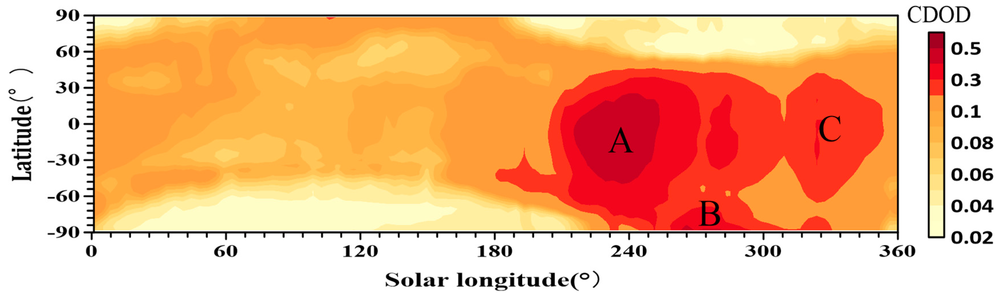
2.1. The Data of CDOD

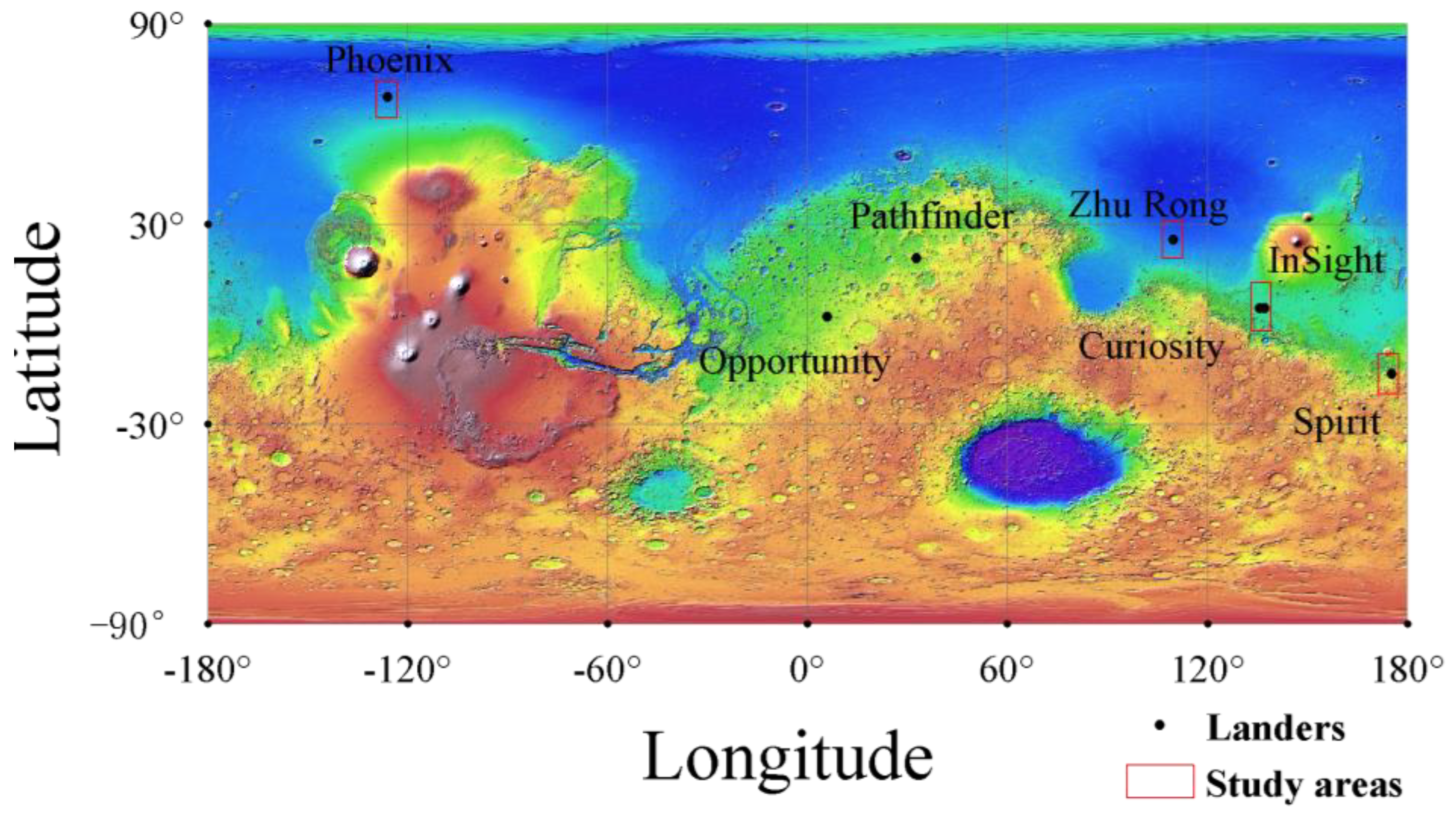
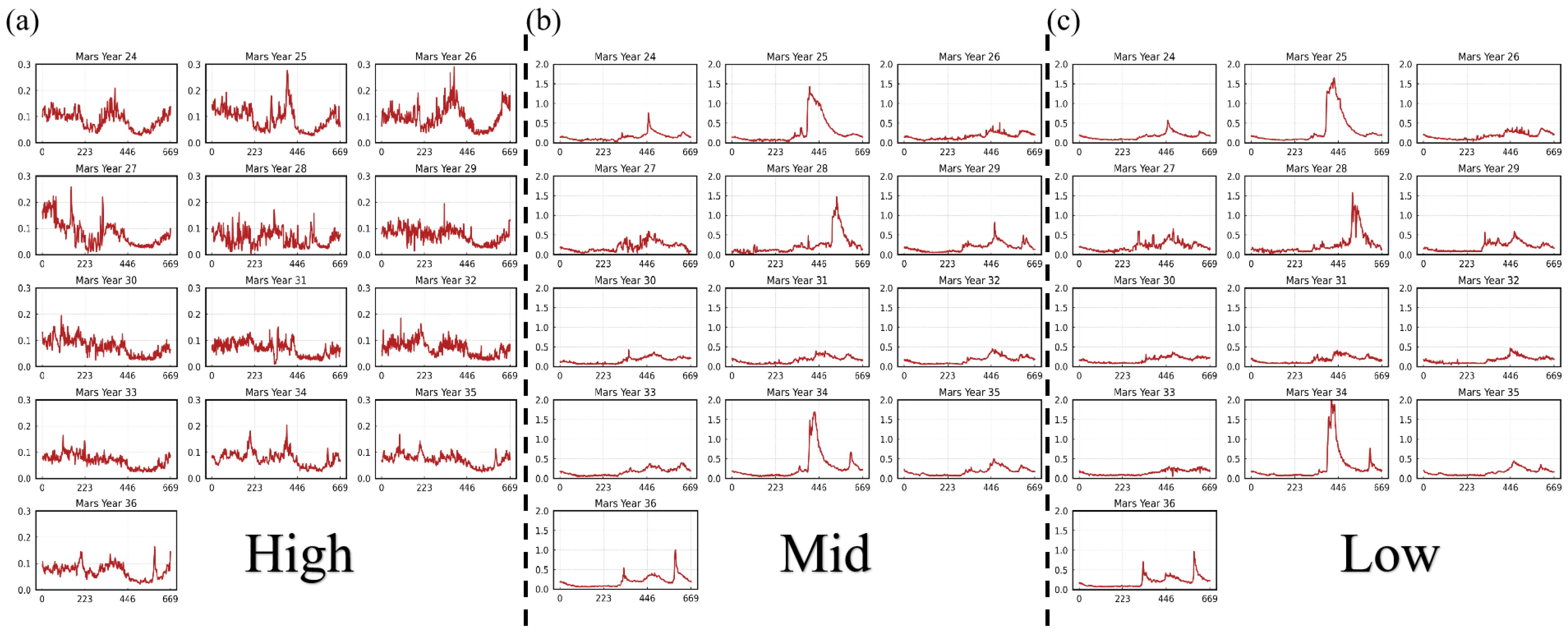
The dust cycle in the Martian atmosphere is considered to be a key process that controls the seasonal and shorter-term weather in the Martian climate. Column Dust Optical Depth (CDOD) is a crucial parameter for quantifying the spatial distribution of mineral dust, reflecting dust concentration changes and serving as a reference for evaluating dust storm occurrences [26]. It can be used as an indicator of dust levels in the atmosphere and a reference for evaluating dust storm occurrences [27]. Through the continuous monitoring of CDOD, scientists can track dust variability across time and space and provide critical support for Martian climate studies and future exploration missions.

In this study, we use the version 6.1 CDOD dataset from the Mars Climate Database (MCD) as equivalent data for characterizing Martian dust storm activity [6]. The MCD utilizes observations from the Thermal Emission Spectrometer (TES) on the Mars Global Surveyor, the Thermal Emission Imaging System (THEMIS) on the Mars Odyssey, and the MCS on the Mars Reconnaissance Orbiter. Currently, the MCD provides global CDOD data with a temporal resolution of 24 h from MYs 24 to 36. Additionally, the data are interpolated from irregular grids to 3° × 3° in latitude and longitude using the Kriging method.

Figure 1 shows the zonal mean CDOD at 610 Pa on the atmospheric pressure surface during MYs 24 to 36 (July 1998 to January 2023). It can be seen that Martian dust storms exhibit typical seasonal variations: from solar longitude (Ls) 0° to 140°, Mars experiences a non-dust storm season, during which dust storm activity is relatively weak; from Ls 140° to 360°, Mars enters the dust storm season, characterized by frequent and intense dust storm activities, particularly between latitudes −90° and 50° [28]. According to the seasonal and temporal characteristics, the three types of dust storms, A, B, and C, are presented in Figure 1. Type-A dust storms occur after the southern hemisphere spring equinox of each Martian year, after Ls 180°, with frequent activity in mid-to-low latitudes and lasting up to four months. Type-A storms have the longest duration, the widest coverage, and the greatest intensity and have the most significant impact on the Martian rover activities. Towards the end of Type-A storms, Type-B storms erupt in the southern polar region, lasting about two months and mainly active in high southern latitudes. Following the end of Type-A and -B storms, Type-C storms occur around Ls 330°, lasting approximately one month, before conditions calm down and the cycle repeats in the next MY.

2.2. Study Areas

The study areas were selected mainly based on the sites of successfully landed probes in previous years, while considering different longitudes and latitudes and different hemispheres to ensure that the areas are as diverse as possible. Each area is defined by expanding the latitude and longitude of the lander by 5–7°. This small area eliminates the need for modeling larger areas, which can reduce the computation cost and receive high-precision prediction. The locations of several important Mars landers are shown in Figure 2. The landing sites of Opportunity, Curiosity, and InSight are located in the equatorial region; Zhurong, Spirit, and Mars Pathfinder are located in the tropics; and Phoenix is located in a high-latitude area. Therefore, four study areas are divided, and the location and range of each area are shown in the red rectangular in Figure 2 and

Table 1. Information of the four selected study areas.

	Latitude Range	Longitude Range	Probe
Equatorial region	7.5°S~7.5°N	132°E~138°E	Curiosity, InSight
South tropical region	10.5°S~22.5°S	171°E~177°E	Spirit
North tropical region	16.5°N~28.5°N	120°E~126°E	Zhurong
High latitude region	58.5°N~70.5°N	231°E~237°E	Phoenix

.

3. Time-Series Prediction

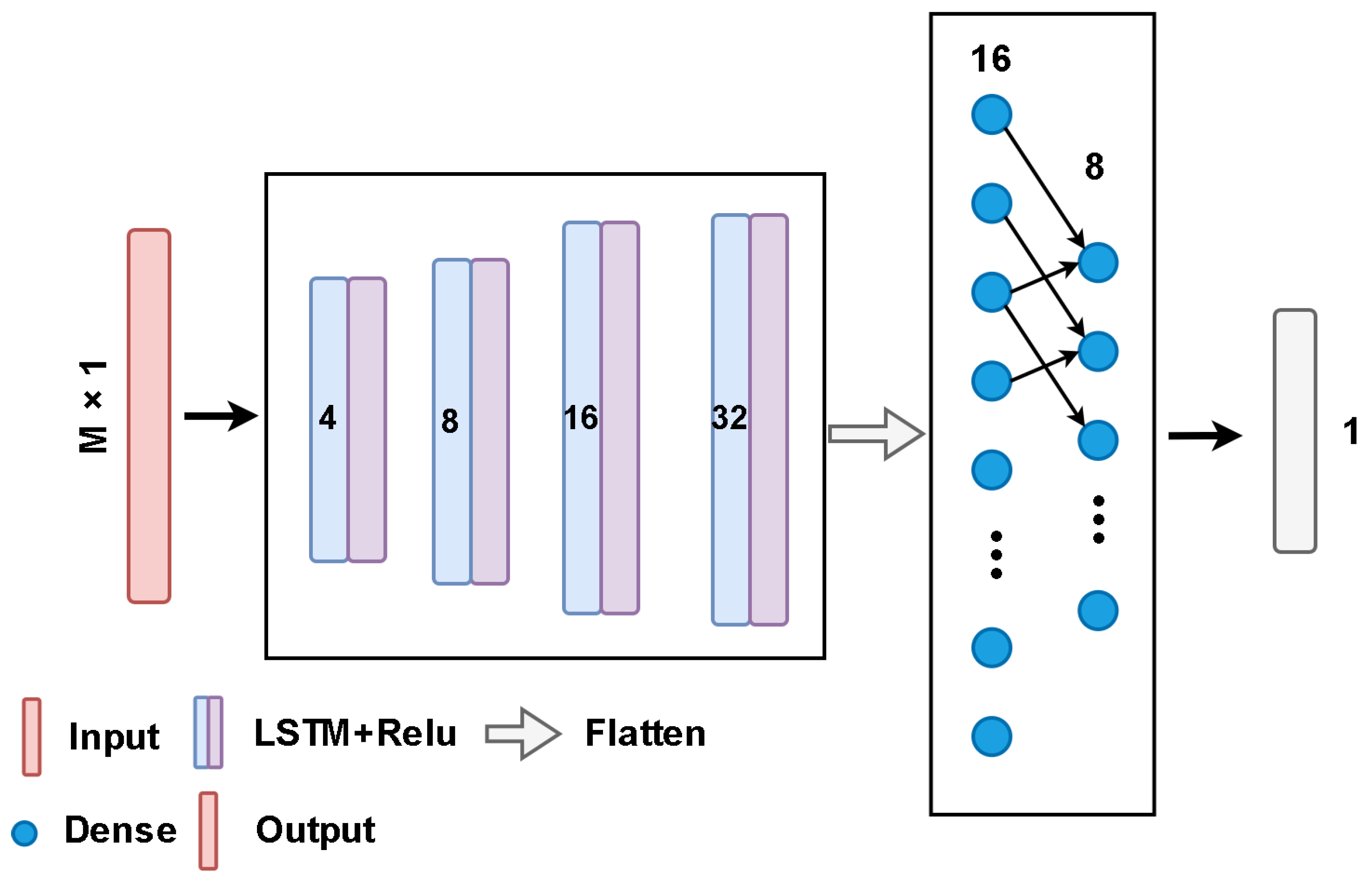
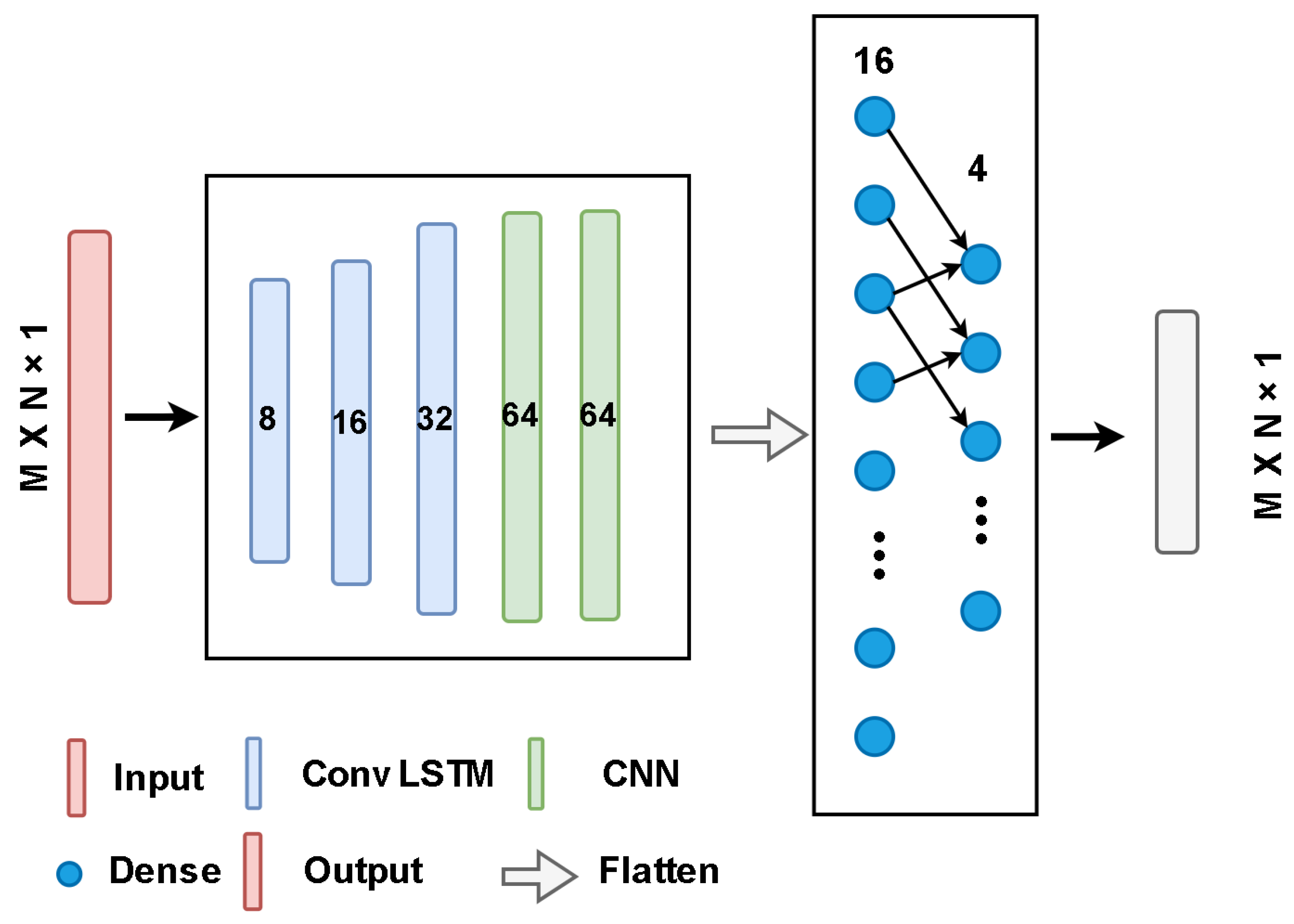
3.1. Model

We use LSTM networks, which are specifically designed for handling time-series information, to predict the CDOD for each Martian sol. Compared to classical Recurrent Neural Networks (RNNs), LSTMs feature a unique gating mechanism that allows them to effectively retain and transmit information across sequences, capturing semantic relationships over long sequences and mitigating issues such as vanishing or exploding gradients [29]. The distinctive gating units of LSTMs enable the network to selectively retain or forget information while processing sequences (Figure 3). At each time step, an LSTM unit receives the current input value and the hidden state from the previous time step. It updates the cell state using values from the input and forget gates. New information is added via the input gate, while old information is retained or discarded according to the forget gate. The output gate’s value, multiplied by the tanh-activated cell state, provides the hidden state for the current time step. This hidden state is then passed to the next layer of the network or used as output.

In this study, we employ a stacked LSTM-Dense architecture (Figure 4) to predict the average CDOD for each sol in the study areas. The architecture consists of multiple LSTM layers followed by fully connected (Dense) layers. The network is designed to learn the temporal features of the CDOD time input sequence over an extended period. The LSTM layers have hidden units that increase progressively: 4, 8, 16, and 32. These layers capture the time-series characteristics of the CDOD data. The learned features are then further processed by two Dense layers with 16 and 8 neurons, respectively, to output the predicted CDOD data for the next sol. Each layer uses the ReLU activation function, and a Dropout layer with a scale factor of 0.1 is added after the last LSTM layer to enhance the network’s generalization ability.

Due to the varying characteristics of CDOD in different Martian regions, the time-step input requirements for networks differ across research areas. To address this, this study employs the Particle Swarm Optimization (PSO) algorithm to search for the optimal time-step length for each region. PSO is originally inspired by the collective behavior of biological groups such as bird flocks or fish schools to find the optimal solution by continuously adjusting the positions and velocities of particles [30]. Here, PSO is utilized to search for the optimal input time window for each research area, ensuring that the network performance is maximized across different regions. During each iteration, each particle updates its position and velocity based on its best-known position both in the search space and of the entire swarm. This process is repeated until the maximum number of iterations is reached. In this study, the search range for the time window is defined in the range of [32 sols, 256 sols], with a swarm size of 10 particles and a maximum of 20 iterations.

3.2. Data Preparation

3.2.1. Data Processing

The data after mean processing in each study area omits spatial features but retains temporal information. However, when predicting purely time-series information, it is necessary to ensure that the data are a stationary, non-random series; otherwise, the prediction accuracy will visibly decrease. Therefore, the following preprocessing steps were applied to the CDOD time series after mean processing: the stationarity test, the pure randomness stationarity test, and normalization.

(1)

Stationarity test: A stationary time series is one whose mean and variance do not change over time. We use the Augmented Dickey–Fuller test to examine the stationarity of the CDOD series [31]. If the test result is a non-stationary time series, first-order difference is applied to transform it into a stationary series.

(2)

Pure randomness stationarity test: Even a stationary time series may exhibit strong randomness, which can evidently affect prediction accuracy. Therefore, the Ljung–Box test is used to verify the pure randomness of the obtained stationary time series, ensuring its non-randomness [31].

(3)

Data normalization: Due to the significant fluctuations in CDOD data caused by global dust storms, the prediction accuracy of the network could be greatly affected. Thus, Min-Max normalization is applied to the processed data, mapping the CDOD values to a range between 0 and 1.

3.2.2. Training Set

Up to now, only the data of MYs 24 to 36 are provided by the MCD database. Directly dividing these data could result in a limited number of trainable samples. Therefore, we perform sliding segmentation on the preprocessed CDOD data to expand the dataset size available for network training. A sliding window approach with a step size of 1 sol is employed: data from sols 1 to x are used to predict the data for sol x + 1; then, data from sols 2 to x + 1 are used to predict the data for sol x + 2, and so forth. Therefore, this approach effectively increases the number of training samples, greatly facilitating network training.

Taking the landing site of Zhurong, north subtropical region in Table 1, as an example, the corresponding network and prediction process are detailed in Section 3.3.1 and Section 3.3.2. The processed CDOD data from MYs 26 to 35 are used as the training and validation sets, with a ratio of 9:1. The CDOD data from MY 36 are used as the test set to evaluate the network’s performance. To minimize the impact of subjective judgment on the dataset, no further distinction between global dust storm and non-global dust storm data is made in the training set.

After data preprocessing and sample preparation for the selected study area, the network model is then trained and tested using these samples. The process is illustrated in Figure 5.

3.3. Model Training and Evaluation

3.3.1. Model Training

The Adam optimizer is used for network training to minimize the loss function. The hyperparameters of the network are set as follows: the learning rate is 1 × 10⁻³, the batch size is set to 64, and the training is performed for 500 epochs. An early stopping strategy is adopted where the training stops if the test set error does not decrease within 20 epochs; this is to prevent overfitting and enhance the generalization ability of the model. The algorithm is implemented on the TensorFlow 2.1 platform, with the following computational environment: Intel(R) Core (TM) i5-10300H CPU @ 2.50 GHz processor and 8 GB RAM.

The prediction performance of the network in the test set is shown in Figure 6. It can be seen that the trained network performs well in predicting the data for MY 36. These results are reflected in the prediction of low CDOD activities in the first half of the year, high CDOD activities in the second half of the year, and the prediction of several CDOD peaks, which are very consistent with the observations. The three evaluation indicators—correlation coefficient (R²), root mean square error (RMSE), and mean relative error (MRE)—are 0.980, 0.188, and 0.035, respectively.

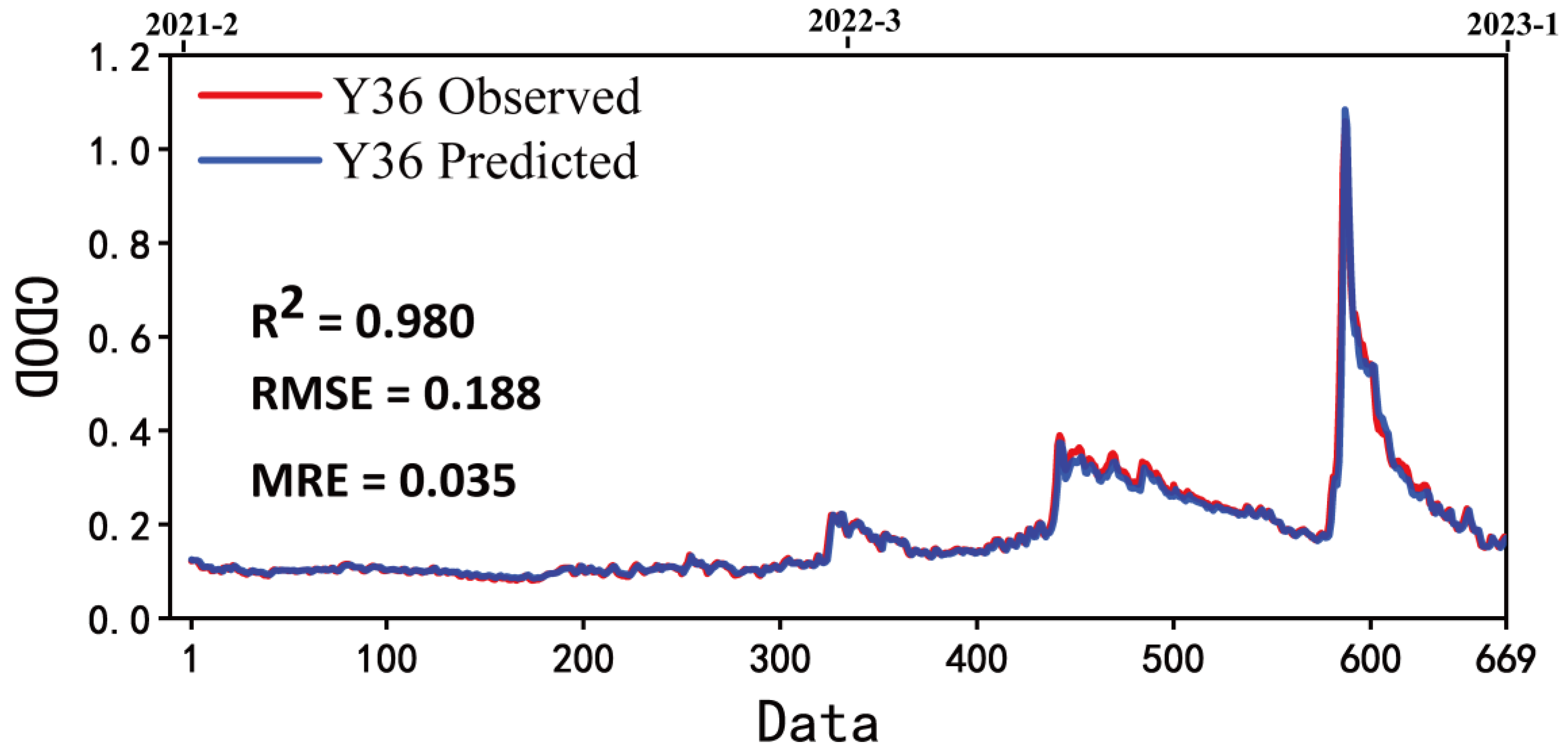
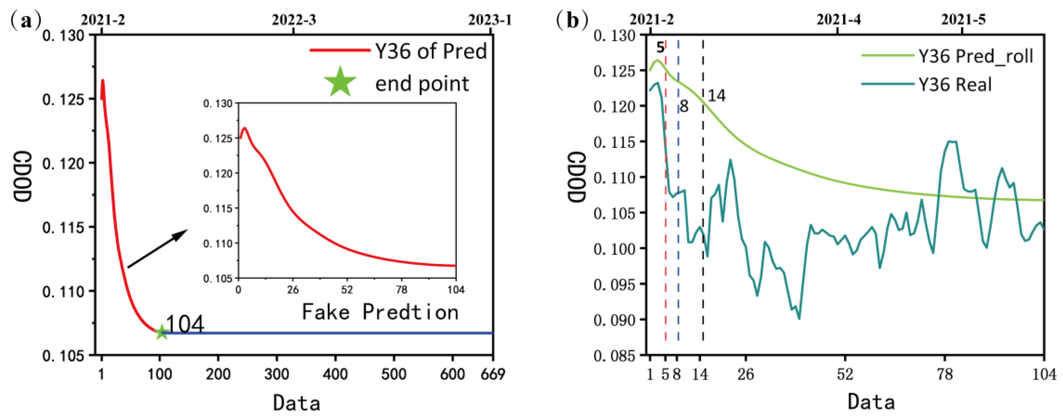
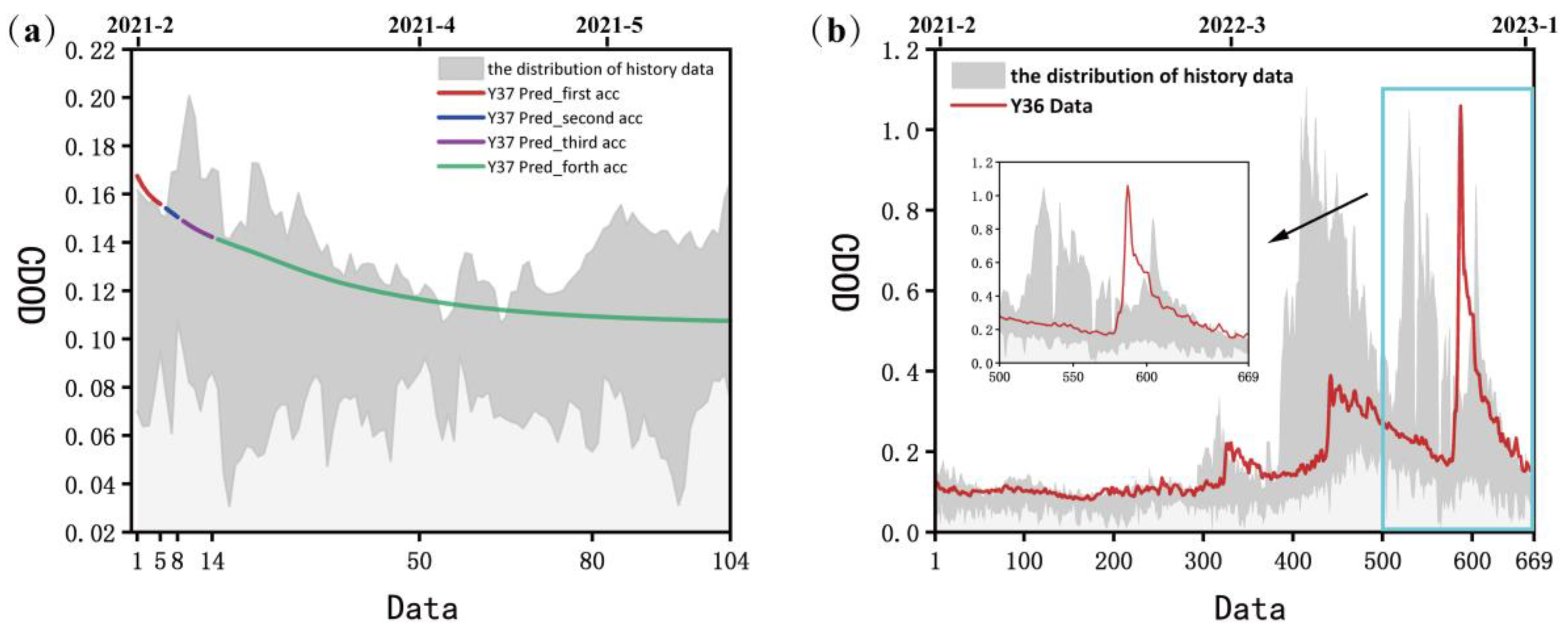
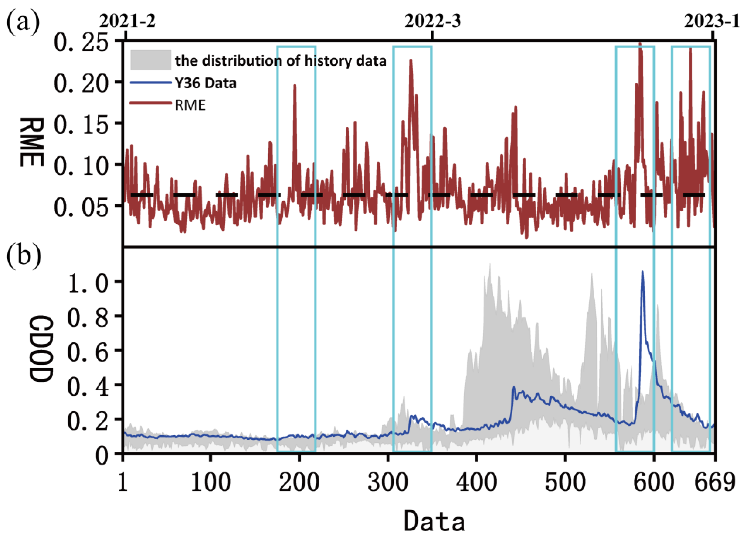
3.3.2. Evaluation Strategy for Rolling Forecast

Since the front of a dust storm can propagate at a speed of 20 to 28 m/s and spread to about 800 km within 12 h, the CDOD in a specific area may undergo notable changes in a short period of time [25]. Therefore, it is not enough to only predict the CDOD for the next Martian sol. However, simply increasing the number of sols predicted by the network will greatly reduce the accuracy of the prediction. As shown in

Table 2. The accuracy evaluation of networks with different output sols on the test set.

	Accuracy	R2	RMSE	MRE
Sols
1		0.980	0.188	0.035
5		0.788	0.299	0.081
10		0.292	0.351	0.111
20		0.027	0.599	0.249

, when the prediction output is extended to 5 sols, the accuracy decreases by approximately 2 times compared to a 1-sol forecast. Then extending the prediction to 20 sols results in a substantial drop in accuracy.

To ensure high prediction accuracy for the next Martian sol and to be able to predict CDOD for more future Martian sols, a rolling prediction strategy is proposed. In this strategy, the prediction for the data from sols 1 to m is incorporated into the input data, and the network then predicts the CDOD from sol m + 1. This process is repeated for continuous rolling predictions. However, since the predicted data inherently contain biases, the prediction error of the network gradually increases, limiting its performance. Therefore, a pre-evaluation strategy based on test set accuracy is applied in this study to determine the maximum number of sols for rolling prediction. The prediction results are divided into four different accuracy intervals to ensure better reference value.

Rolling predictions are performed on the test set, and the results are compared with the observations to determine the maximum number of sols the network can predict. As shown in Figure 7a, after multiple sols of rolling predictions, the network has a low sensitivity to subsequent CDOD data due to accumulated errors in the input data, resulting in an inaccurate prediction. Thus, the minimum adjacent difference between observations on consecutive Martian sols is used as a sensitivity indicator. The maximum number of predictable sols is set as the number of sols where the minimum adjacent difference of the rolling predictions is less than the sensitivity indicator. In Figure 7a, the red line indicates the predictable sols and the blue line indicates fake prediction, that is, the period where the network can no longer make an accurate prediction. The maximum number of sols the network model can predict is 104 sols.

Once the maximum number of sols for rolling prediction is determined, the results are then divided into different accuracy intervals. For this, the rolling prediction data are compared with the cumulative RME and different multiples of RME of the observations and then divided into different accuracy intervals (1 to 4). As shown in Figure 7b, the four different intervals are separated by different colored dashed lines. The highest accuracy interval is from sols 1 to 5, in which the cumulative RME is within the RME of the test set, indicating a high similarity between the rolling predictions and the observations in both trend and value. The other three accuracy intervals are sols 6 to 8, 9 to 14, and 15 to 104, respectively. Comparatively, the second interval has a similar trend but larger value deviations, while in the third interval, the trend changes of some small time segments are not predicted, and the deviation is large; the fourth interval shows similar issues. Overall, the above rolling prediction evaluation strategy is persuasive, which helps to understand the trends of CDOD in future multiple Martian sols.

Figure 8 shows the rolling predictions of the average CDOD values over future multiple Martian sols in the Zhurong study area. In Figure 8a, the gray shaded area represents the range of CDOD values in the past Martian years. It can be seen that the rolling predictions mainly fall within the shaded area, indicating a certain level of confidence in the prediction. Notably, in the first accuracy interval (sols 1 to 5), the prediction (red line) deviates from the historical observation range. Figure 8b shows the average CDOD value of MY 36 (red line) and the range of historical yeas from MYs 24 to 35 in the Zhurong area. It reveals that the amplitude of CDOD in sols 583 to 600 of MY 36 is significantly higher than that of past Martian years, and the amplitude at the end of MY 36 of 640 to 669 sols is also notably close to the upper boundary of historical observations. Therefore, this may cause the predicted CDOD in sols 1 to 5 of MY 37 to be higher than the historical observations in Figure 8a.

3.3.3. Evaluation Across Different Regions

The training and prediction described above are applied to other areas listed in Table 1 to test the generalization of the method, and the prediction metrics are presented in

Table 3. Prediction metrics in different areas.

	R2	RMSE	RME
Equatorial	0.971	0.212	0.045
Tropics	0.981	0.206	0.042
High latitude	0.910	0.278	0.077

. It can be seen that the lowest prediction accuracy is in the high-latitude region with an RMSE of 0.278, while the highest accuracy is in the mid-latitude region has an RMSE of 0.206.

Table 4. Prediction capability metrics in different areas.

	Equatorial	Tropics	High Latitude
max_sols	97	79	106
first_acc	1~18	1~9	1
second_acc	19~97	10~18	2
third_acc	--	19~28	3
forth_acc	--	29~79	4~106

provides the prediction capability metrics of the four different areas, which shows that the effective prediction time of the model is about 100 sols. Specifically, the performance in the equatorial region is the best, not only reflected in the number of the maximum predictable sols (97 sols) but also in the number of the sols within the first and second precision intervals. Although the maximum effective predictable sol is the longest (107 sols) in the high latitudes, almost of them are in the fourth precision intervals. The reasons for the differences in the prediction performance in the different latitudes are discussed in session 5.

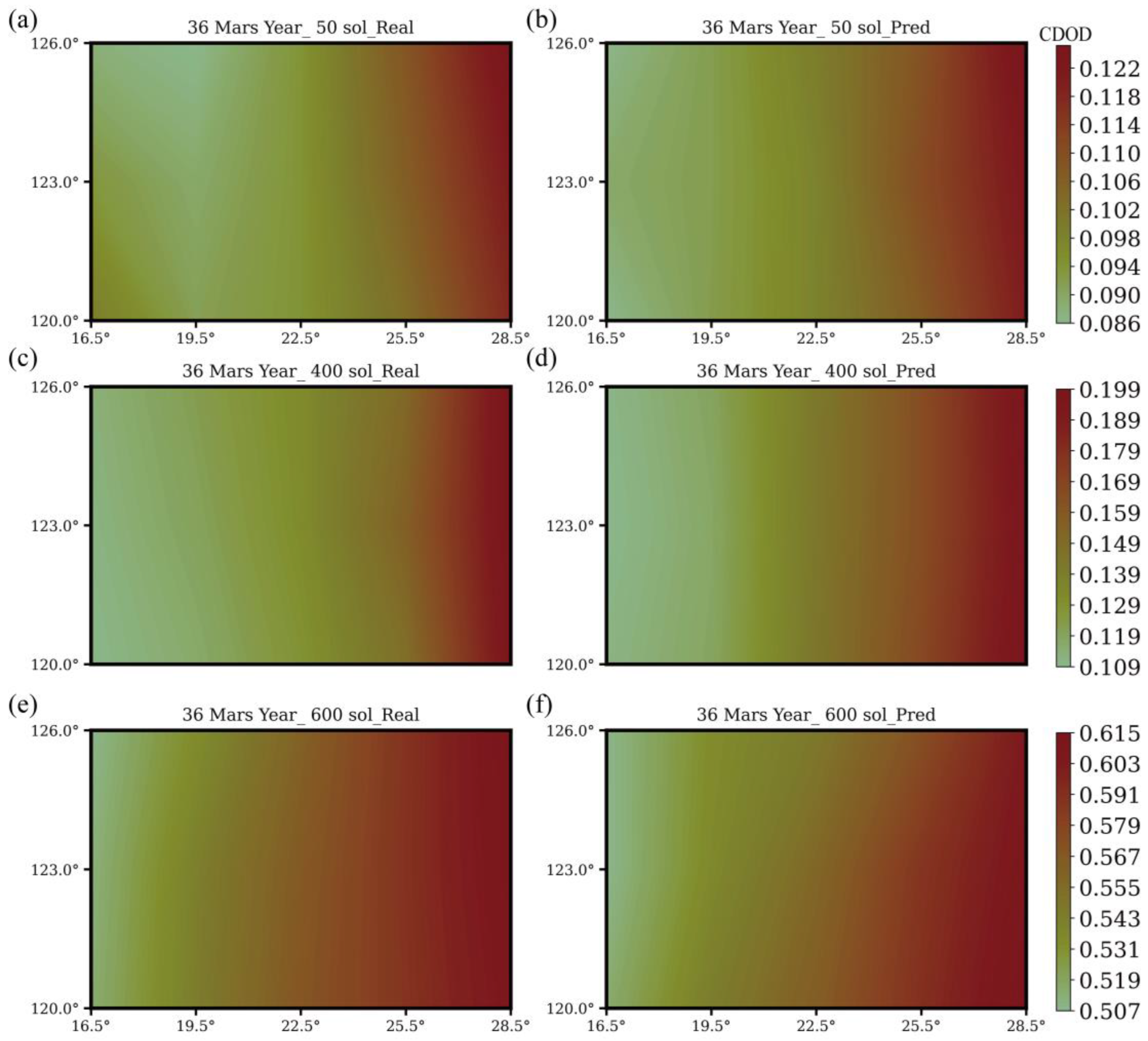
4. Spatial Distribution Prediction

4.1. Model

In addition to the above time-series predictions, we employ a ConvLSTM-based method to predict the spatial distribution of CDOD in the study areas for the next sol. The LSTM network is sensitive to time-series features but cannot fully capture the spatial features of the data. The ConvLSTM network replaces the fully connected layers in the LSTM network with convolutional layers and introduces spatial correlations into the LSTM through convolutional operations, thereby enabling the network to capture both spatial and temporal features of the data simultaneously. Thus, the ConvLSTM network is particularly suitable for handling spatiotemporal sequential data [32].

The network architecture of ConvLSTM used in this study is illustrated in Figure 9. Initially, three layers of ConvLSTM are stacked to extract and learn the spatiotemporal features of CDOD data. The convolutional kernel sizes are set to 3 × 3, with 8, 16, and 32 kernels, respectively. Subsequently, two layers of 2-D convolution blocks process and learn the extracted spatiotemporal features, which are then input to the final fully connected layer. The convolutional kernel sizes and numbers are both set to 3 × 3 and 64, respectively. After processing through two fully connected layers with 16 and 4 neurons, respectively, the output is the spatiotemporal distribution of CDOD for the next sol. ReLU activation functions are employed in each network layer.

The input time window of the network is defined as the CDOD data of 16 sols in the study areas, and the output is the data for the next sol. The Adam optimizer is used for network training to minimize the loss function, with the following hyperparameters: the learning rate is 1 × 10⁻³, the batch size is set to 64, and the training is performed for 500 epochs. Similarly, an early stopping strategy is adopted during training, whereby the error on the test set does not decrease within 20 epochs to prevent overfitting and enhances the generalization ability of the model.

4.2. Model Training and Evaluation

In this section, we continue to take the Zhurong rover landing site as an example to detail the network and prediction process. To enhance the effectiveness of network training, we perform Min-Max normalization on the data, mapping the CDOD data to a range of 0–1. The data division remains consistent with Section 3.2.2, where the processed CDOD data from MYs 24 to 35 are used as the training and validation sets, split in a 9:1 ratio. The CDOD data from MY 36 are used as the test set to evaluate the performance. The entire process is illustrated in Figure 10.

The prediction performance of the network in the test set is illustrated in Figure 11. The two evaluation indicators, RMSE and MRE, are 0.297 and 0.065, respectively. As shown in Figure 11a, the RMSE in the test set reveals high errors around the 200th, 320th, and 600th sols. Comparing these with the CDOD values for each sol of MY 36, as shown in Figure 11b, we can see that the CDOD values at these sols are higher than the historical data from MYs 24 to 35. These anomalies contribute to the lower prediction accuracy during these periods.

To further validate the network’s performance, we predict the CDOD at different periods of MY 36, categorized as early, middle, and late stages (as shown in Figure 12). Figure 12a,c,e show the spatiotemporal distribution of CDOD in the Zhurong region on the 50th, 400th, and 600th sols of MY 36, respectively. Corresponding predictions from the network are shown in Figure 12b,d,f. We can observe that the distribution of real CDOD and predicted CDOD is highly similar, particularly in regions with high CDOD values, which reveals that the network accurately predicts the CDOD across different areas of the research region and provides precise spatiotemporal predictions for high CDOD values.

5. Discussion

Table 5. Prediction metrics in different study areas.

Time Series/Spatial Distribution	RMSE	RME
Equatorial	0.212/0.315	0.045/0.072
Tropics	0.206/0.297	0.042/0.080
High latitude	0.278/0.428	0.077/0.125

presents the evaluation metrics, including RMSE and RME, for the time-series and spatial distribution predictions in different latitudes. It can be seen that the accuracy in the tropics and equatorial region is generally high, with the highest accuracy in the tropics. The RMSE and RME for the time-series/spatial distribution prediction in the tropics are 0.206/0.297 and 0.042/0.080, respectively. In comparison, the accuracy in high latitudes is relatively lower, with an RMSE and RME of 0.278/0.0428 and 0.077/0.0125. Further, the average CDOD of the three different areas over the years (MYs 24 to 36) is shown in Figure 13. It is evident that the average CDOD exhibits consistent distribution patterns in the tropics and equatorial region, while the distribution in the high-latitude areas is irregular, which leads to lower prediction accuracy in this region. Therefore, when applying the model to new areas, it is important to first analyze the temporal CDOD distributions and avoid regions with unclear patterns.

Wei et al. [15] used different methods, including probability analysis, neural network prediction, and the Mars Global Climate Model to predict the CDOD trends at the landing site of China’s Zhurong rover in 2022. The results demonstrate that the global dust storm at the landing site of Zhurong could occur with high incidence from March to December 2022, which could significantly impact the operation of Zhurong. The predictions in this study (Figure 6) also show the increased trends of the dust storms in the Zhurong area after March 2022, especially the Type-C storm around 600 sols. He et al. [25] applied a Convolutional Gated Recurrent ConvGRU-Seq2Seq model to forecast the short-term spatiotemporal distribution of global Martian dust storms, achieving a 12 h prediction with promising accuracy. In comparison, our method achieves more regionally detailed predictions with comparable accuracy despite covering a longer time span.

The LTSM model has been used in the study of Martian atmospheric temperature prediction.

Table 6. The predictions of Martian atmospheric temperature based on various forms of LSTM networks.

References	Network	Evaluation Indicators
Eltahan et al. (2020) [21]	LSTM	RMSE: 0.30
Priyadarshini and Puri (2021) [22]	LSTM	MAE: 0.1257
Al-Saad et al. (2022) [24]	Residual CNN-LSTM	RMSE: 0.15

compares the evaluation indicators of various forms of LSTM networks to predict Martian atmospheric temperature in different studies. It can be seen that different forms of LSTM networks have shown high accuracy in predicting Martian atmospheric temperatures. Similarly, the LSTM and Conv-LSTM networks used in this study have also demonstrated good performance in predicting CDOD in Table 5, indicating that LSTM networks play a crucial role in the time-series prediction of Martian climate conditions. However, the limitations of the LSTM network cannot be ignored. In the studies shown in Table 6, the LSTM networks underperformed in the long-term prediction of Martian atmospheric temperature, a challenge that also emerged in this study. This may be related to the LSTM network’s weaker generalization ability, making it difficult to accurately predict unknown conditions over extended periods. To address this, future research will explore the introduction of large network structures such as Transformers and more complex network architectures.

6. Conclusions

The prediction of Martian dust storm activity is important to understand changes in the Martian atmospheric environment and can also provide a scientific basis for assessing the impact on Mars rovers and operations during dust storms. Traditional Martian atmospheric models are insufficient for accurately predicting dust storm trends. This study employs deep learning, specifically LSTM and ConvLSTM networks, utilizing CDOD data to predict both the temporal and spatiotemporal trends of Martian dust storms.

The temporal trend predictions show that the effective prediction time of the model is about 100 sols. The prediction accuracy is higher in the tropics and equatorial region compared to high latitudes, and the accuracy of the Zhurong landing area in the north subtropical region is the highest, with R² and RME values of 0.98 and 0.035, respectively. In contrast, the accuracy of the Phoenix landing area in the high-latitude area is relatively lower, with R² and RME values of 0.91 and 0.077, respectively. Additionally, the spatial distribution predictions show similar results to the time predictions, with higher accuracy in the tropics and equatorial region.

In conclusion, the two tasks designed in this study achieve accurate CDOD predictions and demonstrate good generalizability across different latitudes. The LSTM and ConvLSTM model show the potential to predict daily average CDOD for more future Martian sols and the spatiotemporal distribution of CDOD for the next sol. However, the Mars Climate Database (MCD) version 6.1 limits the time resolution of CDOD data to 24 h intervals, and the data update annually, restricting the real-time usability of the data to the initial 100 Martian sols of the upcoming Martian year. Future research will employ higher-resolution data and more advanced networks to achieve more accurate predictions of Martian dust storms.

References

1. Yiğit, E. Coupling and interactions across the Martian whole atmosphere system. Nat. Geosci. 2023, 16, 123–132. [Google Scholar] [CrossRef]
2. Wang, Y.; Wei, Y.; Fan, K.; He, F.; Rong, Z.; Zhou, X.; Tan, N. The impact of dust storms on Mars surface rovers: Review and prospect. Chin. Sci. Bull. 2022, 68, 368–379. (In Chinese) [Google Scholar] [CrossRef]
3. Cantor, B.A.; James, P.B.; Caplinger, M.; Wolff, M.J. Martian dust storms: 1999 Mars Orbiter Camera observations. J. Geophys. Res. Planets 2001, 106, 23653–23687. [Google Scholar] [CrossRef]
4. Kass, D.M.; Kleinböhl, A.; McCleese, D.J.; Schofield, J.T.; Smith, M.D. Interannual similarity in the Martian atmosphere during the dust storm season. Geophys. Res. Lett. 2016, 43, 6111–6118. [Google Scholar] [CrossRef]
5. Wang, H.; Richardson, M.I. The origin, evolution, and trajectory of large dust storms on Mars during Mars years 24–30 (1999–2011). Icarus 2015, 251, 112–127. [Google Scholar] [CrossRef]
6. Montabone, L.; Spiga, A.; Kass, D.M.; Kleinböhl, A.; Forget, F.; Millour, E. Martian Year 34 Column Dust Climatology from Mars Climate Sounder Observations: Reconstructed Maps and Model Simulations. J. Geophys. Res. Planets 2020, 125, e2019JE006111. [Google Scholar] [CrossRef]
7. He, F.; Wei, Y.; Rong, Z.; Ren, Z.; Yan, L.; Tan, N.; Wang, Y.; Fan, K.; Zhou, X.; Gao, J. Monitoring methods for Martian dust storms. Chin. Sci. Bull. 2023, 68, 2046–2057. [Google Scholar] [CrossRef]
8. Guha, B.K.; Gebhardt, C.; Young, R.M.B.; Wolff, M.J.; Montabone, L. Seasonal and diurnal variations of duststorms in Martian year 36 based on the EMM-EXI database. J. Geophys. Res. Planets 2024, 129, e2023JE008156. [Google Scholar] [CrossRef]
9. Rong, Z.; Wei, Y.; He, F.; Gao, J.; Fan, K.; Wang, Y.; Klinger, L.; Yan, L.; Ren, Z.; Zhou, X.; et al. The orbit schemes to monitor Martian dust storms: Benefits to China’s future Mars missions. Chin. Sci. Bull. 2023, 68, 716–728. [Google Scholar] [CrossRef]
10. Gichu, R.; Ogohara, K. Segmentation of dust storm areas on Mars images using principal component analysis and neural network. Prog. Earth Planet. Sci. 2019, 6, 19. [Google Scholar] [CrossRef]
11. Ogohara, K.; Gichu, R. Automated segmentation of textured dust storms on mars remote sensing images using an encoder-decoder type convolutional neural network. Comput. Geosci. 2022, 160, 105043. [Google Scholar] [CrossRef]
12. Pla-García, J.; Rafkin, S.C.R.; Martinez, G.M.; Vicente-Retortillo, Á.; Newman, C.E.; Savijärvi, H.; de la Torre, M.; Rodriguez-Manfredi, J.A.; Gómez, F.; Molina, A.; et al. Meteorological Predictions for Mars 2020 Perseverance Rover Landing Site at Jezero Crater. Space Sci. Rev. 2020, 216, 148. [Google Scholar] [CrossRef] [PubMed]
13. Newman, C.E.; de la Torre Juárez, M.; Pla-García, J.; Wilson, R.J.; Lewis, S.R.; Neary, L.; Kahre, M.A.; Forget, F.; Spiga, A.; Richardson, M.I.; et al. Multi-model Meteorological and Aeolian Predictions for Mars 2020 and the Jezero Crater Region. Space Sci. Rev. 2021, 217, 20. [Google Scholar] [CrossRef] [PubMed]
14. Montabone, L.; Forget, F. On forecasting dust storms on Mars. In Proceedings of the 48th International Conference on Environmental Systems, Albuquerque, NM, USA, 8–12 July 2018. [Google Scholar]
15. Wei, Y.; He, F.; Fan, K.; Rong, Z.; Wang, Y. Preliminary predictions of the dust storm activity at the landing site of China’s Zhurong Mars rover in 2022. Chin. Sci. Bull. 2022, 67, 1938–1944. [Google Scholar] [CrossRef]
16. Cheng, K.; Su, M.; Xue, Y.; Qiu, D.; Li, G. Instantaneous inversion of transient electromagnetic data using machine learning. Acta Geophys. 2024, 72, 3407–34016. [Google Scholar] [CrossRef]
17. Hao, Z.; Liu, S.; Zhang, Y.; Ying, C.; Feng, Y.; Su, H.; Zhu, J. Physics-Informed Machine Learning: A Survey on Problems, Methods and Applications. arXiv 2022, arXiv:2211.08064. [Google Scholar]
18. Lv, P.; Xue, G.; Chen, W.; Song, W. Application of the transfer learning method in multisource geophysical data fusion. J. Geophys. Eng. 2023, 20, 361–375. [Google Scholar] [CrossRef]
19. Deng, F.; Hu, J.; Wang, X.; Yu, S.; Zhang, B.; Li, S.; Li, X. Magnetotelluric Deep Learning Forward Modeling and Its Application in Inversion. Remote Sens. 2023, 15, 3667. [Google Scholar] [CrossRef]
20. Bellutta, D. The Fog of War: A Machine Learning Approach to Forecasting Weather on Mars. arXiv 2017, arXiv:1706.08915. [Google Scholar]
21. Eltahan, M.; Moharm, K.; Daoud, N. Sensitivity of different optimization solvers in LSTM algorithm for temperature forecast over Mars at Jezero Crater landing site. In Proceedings of the 2020 21st International Arab Conference on Information Technology (ACIT), Giza, Egypt, 28–30 November 2020; pp. 1–5. [Google Scholar] [CrossRef]
22. Priyadarshini, I.; Puri, V. Mars weather data analysis using machine learning techniques. Earth Sci. Inform. 2021, 14, 1885–1898. [Google Scholar] [CrossRef]
23. Alshehhi, R.; Gebhardt, C. Detection of Martian dust storms using mask regional convolutional neural networks. Prog. Earth Planet. Sci. 2022, 9, 4. [Google Scholar] [CrossRef]
24. Al-Saad, M.; Aburaed, N.; al Mansoori, S.; Mansoor, W.; Al-Ahmad, H. A Study on Deep Learning Approaches for Mars Weather Forecasting. In Proceedings of the 2022 5th International Conference on Signal Processing and Information Security, ICSPIS 2022, Dubai, United Arab Emirates, 7–8 December 2022. [Google Scholar] [CrossRef]
25. He, Z.; Zhang, J.; Sheng, Z.; Tang, M. Deep learning-based 12-hour global dust distribution forecasting on Martian. Rev. Geophys. Planet. Phys. 2024, 55, 479–492. [Google Scholar] [CrossRef]
26. Clancy, R.T.; Wolff, M.J.; Whitney, B.A.; Cantor, B.A.; Smith, M.D.; McConnochie, T.H. Extension of atmospheric dust loading to high altitudes during the 2001 Mars dust storm: MGS TES limb observations. Icarus 2010, 207, 98–109. [Google Scholar] [CrossRef]
27. Montabone, L.; Forget, F.; Millour, E.; Wilson, R.J.; Lewis, S.R.; Cantor, B.; Kass, D.; Kleinböhl, A.; Lemmon, M.T.; Smith, M.D.; et al. Eight-year climatology of dust optical depth on Mars. Icarus 2015, 251, 65–95. [Google Scholar] [CrossRef]
28. Forget, F.; Montabone, L. Atmospheric Dust on Mars: A Review. In Proceedings of the 47th International Conference on Environmental Systems, Rome, Italy, 16–20 July 2017. [Google Scholar]
29. Song, X.; Liu, Y.; Xue, L.; Wang, J.; Zhang, J.; Wang, J.; Jiang, L.; Cheng, Z. Time-series well performance prediction based on Long Short-Term Memory (LSTM) neural network model. J. Pet. Sci. Eng. 2020, 186, 106682. [Google Scholar] [CrossRef]
30. Shami, T.M.; El-Saleh, A.A.; Alswaitti, M.; Al-Tashi, Q.; Summakieh, M.A.; Mirjalili, S. Particle Swarm Optimization: A Comprehensive Survey. IEEE Access 2022, 10, 10031–10061. [Google Scholar] [CrossRef]
31. Liu, H.; Lei, D.; Yuan, J.; Yuan, G.; Cui, C.; Wang, Y.; Xue, W. Ionospheric TEC Prediction in China Based on the Multiple-Attention LSTM Model. Atmosphere 2022, 13, 1939. [Google Scholar] [CrossRef]
32. Shi, X.; Chen, Z.; Wang, H.; Yeung, D.Y.; Wong, W.K.; Woo, W.C. Convolutional LSTM network: A machine learning approach for precipitation nowcasting. Adv. Neural Inf. Process. Syst. 2015, 1, 802–810. [Google Scholar]
Figure 1. The distribution of the zonal mean CDOD variations at an atmospheric pressure level of 610 Pa during MYs 24 to 36. The letters A, B, and C represent three types of dust storms, respectively.
Remotesensing 17 01472 g001
Figure 2. Locations of Mars landers and study areas.
Remotesensing 17 01472 g002
Figure 3. Basic structure of an LSTM network. A represents the same structure as the middle part.
Remotesensing 17 01472 g003
Figure 4. LSTM network structure.
Remotesensing 17 01472 g004
Figure 5. CDOD time-series prediction processing flowchart.
Remotesensing 17 01472 g005
Figure 6. The predicted (blue line) and observed (red line) CDOD of Zhurong site in MY 36.
Remotesensing 17 01472 g006
Figure 7. The rolling predictions of the network for the test set (a) and the comparisons with the observations (b) for MY 36 in the Zhurong study area.
Remotesensing 17 01472 g007
Figure 8. (a) The rolling predictions for MY 37 and (b) the observations in MY 36 of the average CDOD values in the Zhurong region.
Remotesensing 17 01472 g008
Figure 9. ConvLSTM network diagram.
Remotesensing 17 01472 g009
Figure 10. Flowchart of the spatiotemporal prediction process for CDOD.
Remotesensing 17 01472 g010
Figure 11. The (a) RME and (b) mean of CDOD distribution in MY 36. The blue box in the figure highlights the section with relatively larger errors.
Remotesensing 17 01472 g011
Figure 12. Comparison of the observed and predicted spatiotemporal distributions of the network at different sols in MY 36: (a,c,e) the spatiotemporal distributions for the Zhurong rover region on sols 50, 400, and 600 of MY 36, respectively; (b,d,f) the corresponding network predictions.
Remotesensing 17 01472 g012
Figure 13. Average distribution time graphs of Martian CDOD over the years in (a) high latitude, (b) mid-latitude, and (c) low-latitude regions.
Remotesensing 17 01472 g013